A Kitting-Oriented Collaborative Order Reallocation Method for Large-Scale Manufacturing

Abstract

The leading enterprise-dominated collaborative production mode has become a major trend in large-scale manufacturing, which poses significant challenges to cross-enterprise resource kitting and efficient production collaboration among multiple suppliers. However, for kitting, current research mainly focuses on in-house material assembly kitting, largely overlooking cross-enterprise order production kitting. Traditional order reallocation methods often ignore kitting characteristics, thereby hindering dynamic and sustainable collaboration. To address these gaps, this study proposes a novel kitting-oriented collaborative order reallocation method. This method integrates kitting with order reallocation techniques, characterizes the large-scale collaborative production mode, and establishes a dynamic collaborative control framework. A kitting-oriented multi-objective order reallocation model is then developed, which explicitly incorporates kitting and cost objectives to balance economic efficiency with supply chain stability. An improved Non-Dominated Sorting Genetic Algorithm-II with Repair Mechanism (NSGA-II_RM) is designed, featuring novel chromosome repair and initial population generation operations. Finally, case studies and comprehensive comparative analyses are conducted to validate the feasibility and effectiveness of the proposed method. The results demonstrate its great potential in addressing dynamic cross-enterprise order reallocation and resource kitting problems, while balancing solution quality, computational efficiency, and scalability.

1. Introduction

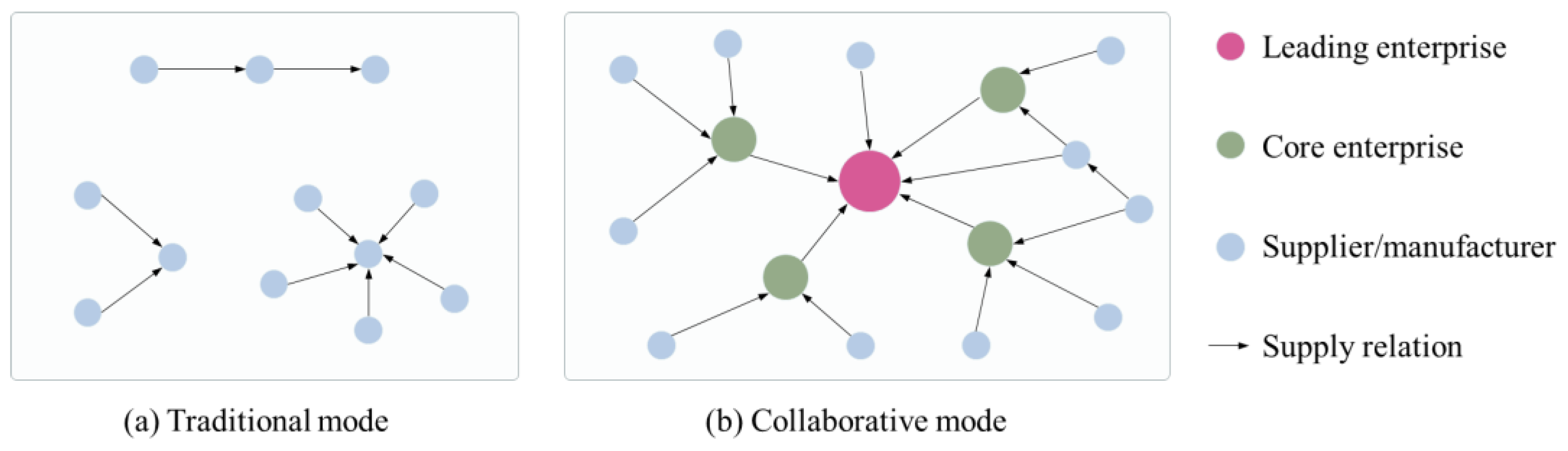
Currently, with the rapid advancement of the new technological and industrial revolution, global manufacturing enterprises, especially large-scale manufacturing industries such as home appliances and automobiles, are increasingly moving toward centralization, networking, and collaboration. The supply chain, comprising suppliers and manufacturers, is evolving from a single-point, single-chain, and localized hierarchical interaction mode to a multi-point, multi-chain, and globally networked collaboration mode [1], as illustrated in Figure 1. In this mode, some end-product manufacturers leverage digital, networked, or intelligent technologies to enhance their collaborative influence and control roles [2,3]. This development urges them to evolve into leading enterprises, such as Gree Electric Appliances [4] and Tesla, Inc. [5]. Other related suppliers or manufacturers engage in corresponding business activities around these leaders and are subject to their supervision or control, thus forming a collaborative network mode (abbreviated as “collaboration mode”). Under this mode, significant challenges arise, such as complex dependencies, collaborative mechanisms, and collaborative management. Therefore, how to effectively leverage the collaborative effects, reduce collaborative costs, and improve collaborative efficiency and performance has become a primary focus in both academia and industry.

Kitting refers to ensuring the completeness of materials before product assembly; it requires that all assembly materials are complete and that their quantities are properly matched [6,7]. In traditional research, kitting mainly focuses on in-house material kitting. Such studies consider production rhythm, batch size [8], operator reaction [9], and inventory information [10] for materials preparation to meet in-house collaboration processes. However, with the evolution of the collaboration mode, as illustrated in Figure 1, material kitting is inadequate to meet cross-enterprise collaboration needs. This has led to the emergence of order production kitting (namely, order kitting). Order kitting focuses on coordinating order fulfillment across enterprises, aiming to meet customer demand and production delivery requirements by ensuring that all delivered materials from suppliers can be assembled within the required time. The concept is in line with the collaboration mode. Thus, in recent years, some scholars have begun to consider the roles of order kitting in collaborative production. For example, Pan et al. [11] classified kitting into three categories, namely, pre-production logistics kitting, in-production logistics kitting, and post-production logistics kitting, where the post-production logistics kitting emphasizes kitting orders for delivery to customers. Ostermeier, Jaehnert, and Deuse [12] considered the joint modeling of the order-dependent parts supply strategies with kitting. Bo et al. [13] integrated the order delivery kitting into collaborative scheduling among supply chain enterprises. Currently, order kitting has attracted wide attention. However, most studies focus on a few enterprises or local collaborations. The systematic and overall collaboration methods have not been fully explored, especially in the large-scale collaboration mode. Moreover, the dynamic characteristics are not fully considered and integrated into the order kitting processes. This hinders the development of order kitting.

Meanwhile, in cross-enterprise collaboration, a feasible and effective order allocation scheme is critical to ensure effective collaboration. In particular, when dynamic disturbances occur, the planned collaboration is disrupted [14,15]. It is essential to determine how to adjust the allocation scheme to enable the subsequent collaboration. In this process, the order reallocation method has been widely studied [16,17]. Research has considered various disturbance uncertainties, allocation rules, allocation requirements, and allocation objectives to determine the optimal dynamic adjustment scheme for order quantity. However, order kitting is rarely applied in the order reallocation process. The combined characteristics, objectives, constraints, and control processes have not been fully revealed. This leads to insufficient kitting and poses challenges in ensuring effective collaboration.

Overall, to address the above shortcomings, it is necessary to study dynamic order kitting and reallocation problems. The order kitting requirements and dynamic characteristics need to be integrated into the dynamic reallocation process to determine the optimal reallocation scheme relative to the initial static allocation scheme. Thus, this study proposes a kitting-oriented collaborative order reallocation method. Firstly, the collaborative framework is presented, integrating kitting and reallocation problems. Secondly, the detailed reallocation model is constructed, which integrates kitting objectives, kitting constraints, and initial allocation schemes. Then, the improved Non-Dominated Sorting Genetic Algorithm-II with Repair Mechanism (NSGA-II_RM) is proposed to solve the model. Finally, the case study and comparative analyses are conducted to verify the model. The main innovations and contributions are as follows:

• This research proposes a large-scale collaborative production mode and constructs a kitting-oriented dynamic collaborative control framework. It integrates order kitting, order reallocation, and cross-enterprise collaboration within the supply chain.
• This paper proposes a kitting-oriented multi-objective order reallocation model. It integrates the kitting-related objectives and constraints, as well as the dynamic disturbances and initial allocation schemes. Meanwhile, an improved NSGA-II_RM algorithm is developed, incorporating a novel chromosome repair mechanism and initial population generation operations. The optimal reallocation results can be obtained.
• The actual application cases and comprehensive comparative analyses are conducted to obtain experimental results. The results and discussion reveal that the proposed method can determine the optimal reallocation scheme and demonstrate superior performance in convergence, uniformity, and generality. The method also shows advantages in balancing solution quality, computational efficiency, and scalability. Moreover, management insights for order reallocation implementation are provided. The feasibility and effectiveness of the proposed method are thus verified.

The rest of the paper is organized as follows: Section 2 reviews the related research. Section 3 presents the proposed collaboration mode and collaboration framework, and describes the problem. In Section 4, the kitting-oriented order reallocation model is built, and in Section 5, an improved NSGA-II_RM algorithm is proposed. The case study, analysis, and discussion are presented in Section 6. Finally, Section 7 draws together the conclusions of this study.

2. Literature Review

2.1. Kitting Collaboration

Kitting collaboration arises from the study of material kitting and order kitting [11]. In material kitting, Wang [8] introduced the fundamental concepts and development of kitting, proposing a kitting manufacturing model and a kitting coefficient for internal enterprises. They aimed to achieve kitting in the manufacturing process by controlling production rhythm, batch size, and execution rules. Zhang et al. [18] adapted augmented reality to enhance the material kitting in selective assembly. Zhu et al. [19] focused on the assembly production process of air defense missiles and proposed a material kitting time prediction method in a discrete assembly workshop based on digital twins. Montoya-Zapata et al. [9] used a multi-agent systems (MAS)-based methodology to study kitting processes in the automotive assembly line. They aimed to reduce the alert reaction time for missing parts triggered by operators. Simoes, Pinto, and Silva [20] discussed different order picking and kitting systems in the automotive industry, and proposed two kitting optimization methods for hybrid kitting systems. Fatima et al. [10] recognized the importance of the kitting cart in manufacturing and developed a harmonious optimization for kitting cart inventory and labor management.

In order kitting, Bo et al. [13] focused on the collaboration between axle company M and wheel company S. By considering the kitting of orders supplied by S to M and the production disturbances at S, they constructed a collaborative scheduling model for S and M. Pan et al. [11] considered the relationships among suppliers, manufacturers, and customers, proposing a multi-level assembly collaboration framework that covers material kitting, part kitting, and order kitting from suppliers to manufacturers to customers. They developed a collaborative control method based on target cascading in dynamic environments.

Overall, to support supply chain coordination, considering the kitting of orders supplied by suppliers has become a key trend and focus. Meanwhile, some scholars are concerned about the impact of dynamic disturbances on kitting and have tried to explore the dynamic coordinated scheduling or control method considering the objectives or constraints of order kitting.

2.2. Order Allocation Method

In cross-enterprise collaboration, reasonable supplier selection, order allocation, and order reallocation are critical to achieve collaborative goals.

In order allocation, Khoshfetrat, Rahiminezhad, and Almasi [21] considered inflation, risks, and fuzzy uncertainty in the automobile industry to construct a supplier selection and order allocation coordination model. Pajic et al. [15] developed a supplier selection method, with which the order allocation model, combining transport cost, is also applied to further determine which supplier to order goods from and in what quantity. Vaezi, Rabbani, and Yazdian [22] proposed a bi-objective Mixed Integer Linear Programming (MILP) model to derive the final optimal decisions regarding order allocation, which incorporates the cost objects and total supply scores. Chen et al. [23] innovatively integrated the purchase lead time into the multiple material order allocation optimization model, and implemented the optimal allocation with cost, timeliness, and sustainability simultaneously. Xu, Liu, and Huang [24] completed the distribution of manufacturer orders based on fixed allocation rules and proportional allocation rules. Alejo-Reyes, Mendoza, and Olivares-Benitez [25] introduced the perfect rate and capacity of suppliers, and proposed a new heuristic method to solve the selection and allocation problem.

Considering that it is difficult for the static allocation scheme to meet the dynamic requirements, some scholars attempted to realize dynamic coordination through order reallocation. Li et al. [26] combined the actual supply capabilities of suppliers, dynamic time factors, and green environmental factors to develop a dynamic selection and order reallocation model for new energy vehicle manufacturers and their component suppliers. Nazari-Shirkouhi S et al. [27] used robust fuzzy multi-objective programming under conditions of multiple projects, multiple suppliers, multiple price levels, and multiple periods, aiming to determine collaborative allocation strategies for suppliers at different dynamic stages. Islam, Amin, and Wardley [28] considered the demand uncertainty and built a data-driven three-stage solution framework involving demand forecasting, supplier selection, and order allocation planning. Tajally et al. [29] focused on the home appliances industry and incorporated the agility, resilience, and sustainability simultaneously into the data-driven order allocation. Gabellini et al. [30] considered disruption risks and proposed an integrated order reallocation framework, which proactively mitigated risks by reallocating orders to suppliers based on updated predictions. Shi and Zhu [31] integrated supply chain disruption risks and carbon emissions into the high-dimensional multi-objective order reallocation optimization model, and thus implemented the optimal reallocation of the initial allocation strategy.

Learning from the above research, the uncertain, dynamic disruption, various forecasting, and data-driven methods are considered and integrated to enhance the dynamic order allocation or form the reallocation schemes. However, the kitting information is little considered in the reallocation process.

2.3. Research Gaps

In summary, as collaborative modes develop, although some scholars have begun exploring cross-enterprise order kitting and collaborative order reallocation methods, several key gaps remain: (1) Most research focuses on material kitting. However, order kitting in collaboration mode, despite receiving significant attention, is still in its early stages, with limited substantive research. (2) There is a lack of systematic support for effectively integrating disturbance factors into cross-enterprise order kitting and developing a dynamic collaborative control method. (3) The goal of order kitting is decoupled from the order reallocation process, and the reallocation model rarely considers the requirements of order kitting. This leads to insufficient kitting and difficulties in ensuring sustainable collaboration in the supply chain.

3. Collaboration Framework and Problem Description

3.1. Collaborative Production Mode

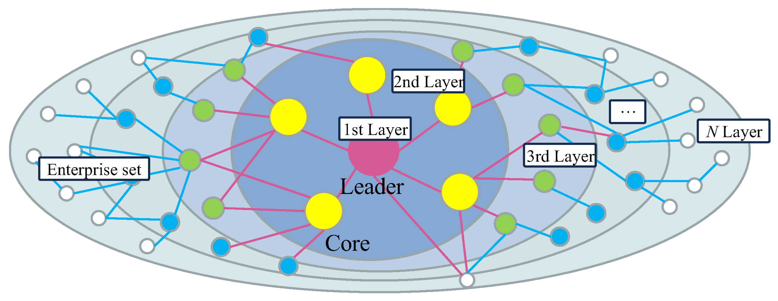
In recent years, with the rapid growth of large-scale manufacturing industries such as home appliances and automobiles, suppliers of raw materials and components, core manufacturers, and end-product manufacturers are increasingly adopting a networked and collaborative production mode [1]. This leads to the emergence of leading enterprises, such as Gree Electric Appliances [4] and Tesla, Inc. [5]. Other companies have gradually become dependent on or associated with these leading enterprises, forming a large-scale collaborative production paradigm, characterized by a single leader, multiple cores, multiple layers, multiple levels, and collaborative production, as illustrated in Figure 2. For example, Gree includes 14 core supporting manufacturing enterprises and more than 3000 related suppliers.

• Specifically:

• Single leader and multiple cores

Single leader: The supply chain leading enterprise or end-product manufacturing enterprise that has a major influence and control ability within the industrial chain.

Multiple cores: The supporting enterprises or one-level suppliers of the leading enterprise that provide core components.

• Multi-layer and multi-level

Multi-layer: The leader is located in the first layer, followed by component suppliers to the leader (2nd layer), then suppliers to these suppliers (3rd layer), and so on. Based on the Bill of Materials (BOM) and component supply relationships, each supplier forms part of a multi-layer supply structure. Notably, some suppliers can serve multiple layers simultaneously, with their level being determined by the highest layer they serve. For example, if Company A supplies components to both Company B in the 2nd layer and Company C in the 3rd layer, then Company A is considered to be in the fourth layer.

Multi-level: A supplier has multiple levels if it provides components to enterprises in multiple layers. For example, if one supplier provides parts for leading enterprises and a 1st level supplier, it is considered both a 1st level and a 2nd level supplier.

Assuming that the enterprise group is represented by E, it can be described as:

$$\left\{\begin{array}{l}E=\{E_1,E_2,\cdots ,E_n\}\\ E_i::=\{{\mathrm{type}}_i,{\mathrm{layer}}_i,{\mathbf{levelset}}_i\}, i\in (1,n)\end{array}\right.$$

(1)

where E_i represents the i-th enterprise; n is the number of enterprises in the group; type_i indicates the category of enterprise E_i, including leading enterprise, core enterprise, and supplier enterprise; layer_i is the level of enterprise E_i; and levelset_i is the set of levels of enterprise E_i.

• Collaborative production

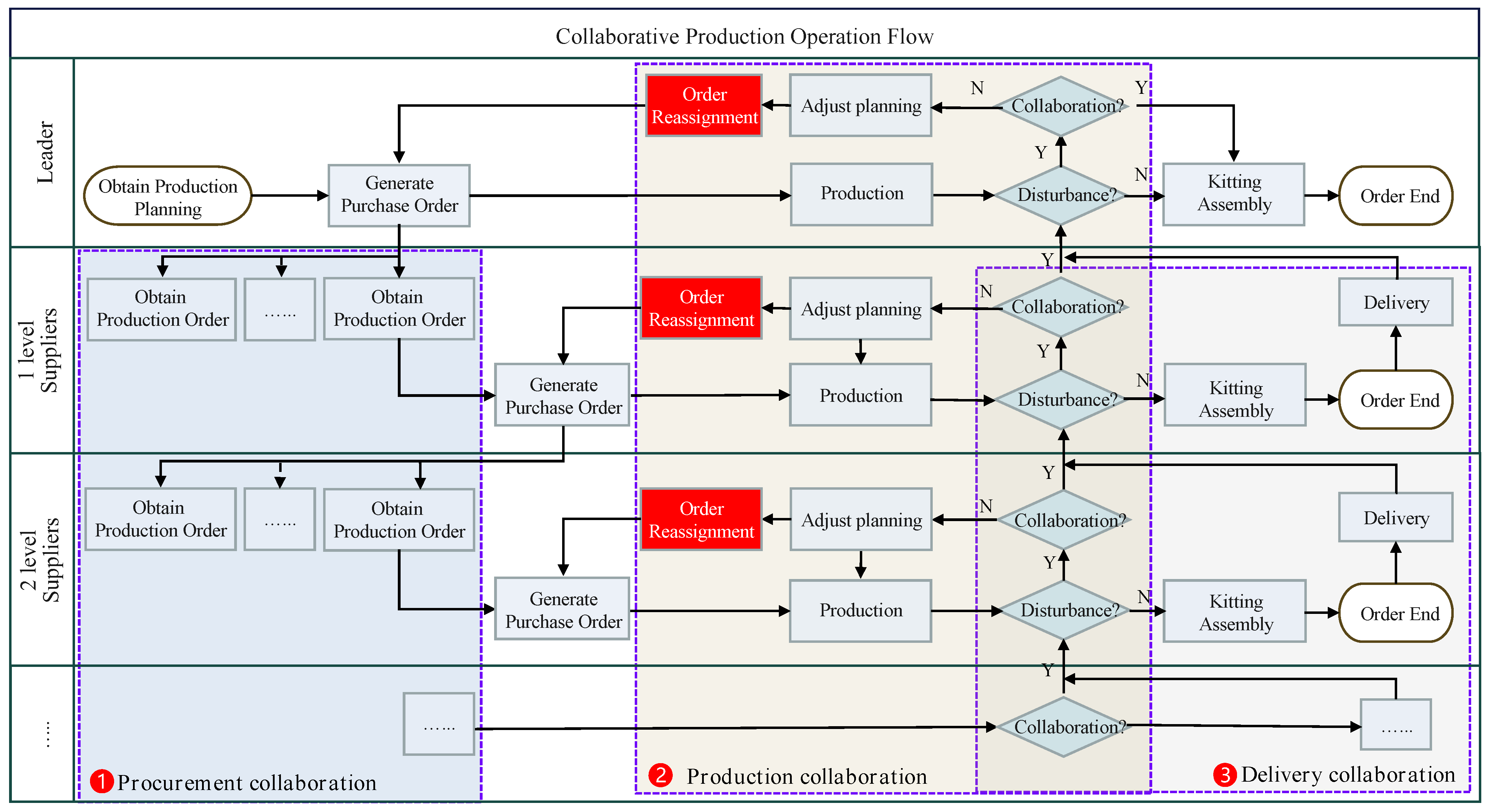
Collaborative production involves procurement collaboration, production collaboration, and delivery collaboration. The detailed collaboration process is illustrated in Figure 3, as follows:

Firstly, to meet assembly needs, the leading enterprise divides and combines orders based on the BOM structure and production planning, forming material procurement orders. These orders are then allocated to the 1st-level suppliers. The delivery quantity and time are set to ensure kitting assembly. After that, the 1st-level suppliers, based on order requirements and their production capacity, purchase materials from the 2nd-level suppliers and set their delivery requirements. The 2nd-level suppliers, based on their order requirements and production capacity, purchase materials from the 3rd-level suppliers and set their delivery requirements, and so on. All the suppliers, guided by the kitting material requirements, form a procurement collaboration process.

Secondly, during the production process, a series of production disruptions, such as equipment failure or material interruptions, could lead to insufficient capacity for suppliers to meet the subsequent kitting requirements. In this case, the suppliers will dynamically adjust their production planning. If the planning cannot be satisfied, the orders could be reallocated to other enterprises. In this process, the production progress could be dynamically obtained to achieve production collaboration among supplier enterprises.

Finally, after completing production, each supplier delivers the required materials to the following enterprise according to the kitting constraints and delivery times. This ensures global assembly kitting and enables delivery collaboration.

3.2. Kitting-Oriented Dynamic Collaborative Control Framework

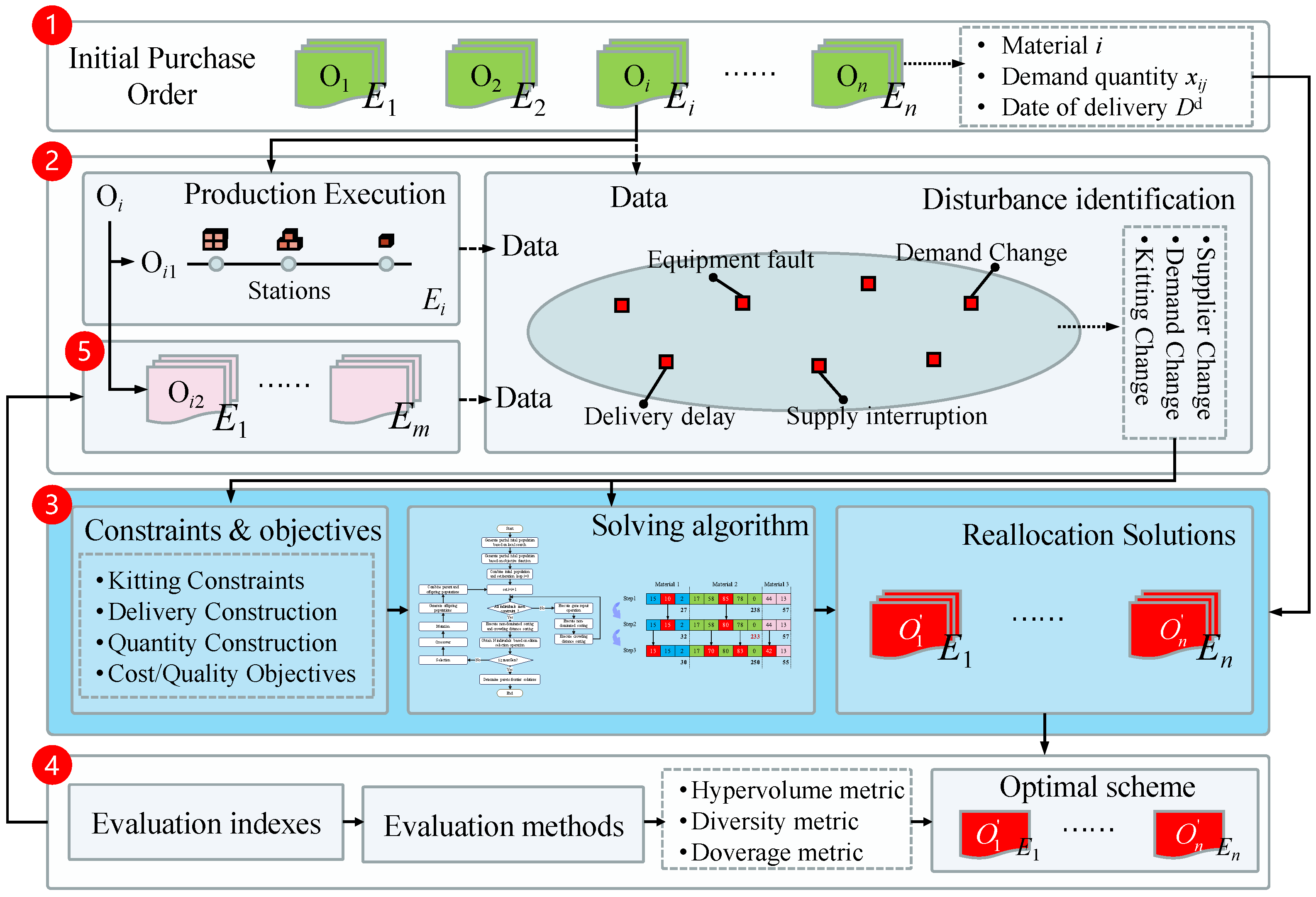
Combined with the above collaboration mode, the order reallocation operations are critical to meet kitting needs and implement dynamic collaboration. This can enable the dynamic adjustment of production plans based on kitting needs, production capacity, and resource conditions, thus ensuring the stability and efficiency of production processes. As shown in Figure 4, the kitting-oriented dynamic collaborative control framework involves initial order acquisition, dynamic disturbances identification, order reallocation implementation, evaluation of optimal allocation schemes, and collaborative control process execution.

• The detailed process is as follows:

• Initial order acquisition: Based on the collaborative production process, the initial order scheme O_i, including allocated material i, demand quantity x_ij, and delivery time D^d for selected supplier E_i, is obtained. This process relies on the supplier selection and order allocation methods, which are not within the scope of this paper.
• Dynamic disturbance identification: After each supplier obtains their orders, production could be executed. In this process, combining production data and collaborative interaction data, the uncertain disturbance information, such as equipment fault, supply interruption, delivery delay, or market changes, could be identified. This information will be applied to reveal the related changes in different enterprises.
• Order reallocation implementation: Based on the above changes, the remaining orders could be adjusted and reallocated relative to the initial allocation schemes. This involves adjustments to kitting, demand, delivery time, order quantity, and suppliers. They can be quantified based on the related constraints and objectives, and thus, the order reallocation models and solution algorithms can be constructed. After solving, feasible dynamic order reallocation schemes for each new order $O_i^{\prime }$ can be determined.
• Optimal allocation schemes evaluation: The above feasible schemes are not the only ones. Corresponding evaluation indicators are constructed for models, algorithms, or solutions to evaluate the rationality and value of the allocation schemes from different dimensions and to determine the optimal recommended reallocation scheme.
• Collaborative control process execution: According to the determined optimal scheme, the initial scheme O_i for supplier E_i will be adjusted to $O_i^{\prime }$. The adjusted order O_ij will be allocated to other suppliers. In this case, the optimal reallocated schemes can be executed, thus realizing collaborative control and meeting subsequent kitting demand.

3.3. Problem Descriptions

Under the collaboration mode and framework, this study focuses on the kitting-oriented order reallocation process. The problem can be described as follows.

On the basis of the kitting requirement, initial scheme, and dynamic disturbance information from multiple enterprises, the problem is how to construct a kitting-oriented order reallocation model and a corresponding solution algorithm. The model needs to consider and integrate cost, quality, and kitting requirements. The algorithm should be able to rapidly obtain the optimal scheme. The scheme is essential to provide the updated order quantities for the selected suppliers for each required material.

Specifically, assuming that I represents the total number of material types in the order, J_i is the number of matched suppliers for each material type M_i, Q_i indicates the quantity demand for material M_i, x_ij is the supplied quantity allocated to supplier j for material M_i, and y_ij indicates whether supplier j is chosen to supply material M_i. After a disturbance occurs, J_i, I, and Q_i may change. This requires the necessary adjustments to x_ij and y_ij to achieve the optimal dynamic collaborative scheme while considering order kitting requirements.

4. Kitting-Oriented Order Reallocation Model

4.1. Model Assumptions

Based on the above framework, the related assumptions are as follows:

• The production of orders is divided into several cycles. In each cycle, the allocation scheme remains unchanged until the next production cycle.
• The reallocation process is applied to the subsequent cycles. Likewise, the initial scheme is derived from the original scheme in the subsequent cycles.
• The supplier’s supply capacity is known, and the supply quantity is determined by the minimum order quantity and maximum supply capacity, which are not changed until the next production cycle.
• The defect rate and delay rate are predetermined and vary across materials for each supplier. They are statistically calculated based on historical sample data.
• Supplier inventory is not considered and is incorporated into the maximum supply capacity.
• The total order demand of the leading enterprise for each material is known, which is determined according to the production capacity, production planning, customer orders, and kitting objectives.

4.2. Model Formulation

Based on the above assumptions, a kitting-oriented order reallocation model is constructed. The relevant notations and definitions are shown in

Table 1. Notations and definitions.

Notations	Definitions
I	The number of material types supplied in the order
Ji	The number of suppliers from which the material Mi can be sourced
$x_{ij}$	The quantity of material Mi allocated to supplier j, xij ∈ ${\mathbb{Z}}_{\ge 0}$
$y_{ij}$	Indicates whether material Mi is supplied by supplier j: 1 if yes, and 0 otherwise
cr	The required kitting rate for the target enterprise (%), 0 ≤ cr ≤ 100%
Ff	Order kitting rate (%), 0 ≤ Ff ≤ 100%
$Q_i$	The total demand quantity of material Mi
l	The unit loss cost due to insufficient kiting quantity
$c_{ij}^{\mathrm{b}}$	Purchase cost of unit material Mi when supplied by supplier j
$c_{ij}^{\mathrm{f}}$	Transportation cost of unit material Mi when supplied by supplier j
$p_{ij}^{\mathrm{dq}}$	The defect rate of material Mi when supplied by supplier j
$p_{ij}^{\mathrm{de}}$	The delay rate of material Mi when supplied by supplier j
$x_{ij}^{\min }$	The minimum order quantity of material Mi when supplied by supplier j
$x_{ij}^{\max }$	The maximum supply capacity of material Mi when supplied by supplier j
$D^{\mathrm{d}}$	The order delivery time
$D_{ij}^{\mathrm{d}}$	The actual delivery time of material Mi when supplied by supplier j
$D_{ij}^{\mathrm{t}}$	The transportation time of material Mi when supplied by supplier j
$t_{ij}^{\mathrm{p}}$	The production time of unit material Mi when supplied by supplier j

.

To achieve kitting requirements and optimal allocation, this paper selects two optimization objectives: minimizing production cost C and minimizing the quantity of non-kitting materials N^L. Specifically:

1.

Minimizing production cost C

To improve production sustainability and reduce losses, the overall production cost is considered. It consists of three parts: the loss cost C^l caused by failing to meet the expected targets, the total purchase cost C^b of all materials, and the total transportation cost C^f of all materials. That is:

$$F1=\min C=\left(C^{\mathrm{l}}+C^{\mathrm{b}}+C^{\mathrm{f}}\right)$$

(2)

where C^l, C^b, and C^f can be expressed as:

$$\left\{\begin{array}{l}{C}^{\mathrm{l}}=l\times (1-F^{\mathrm{f}})\times {\displaystyle \sum _{i=1}^I{Q}_i}\hfill \\ C^{\mathrm{b}}={\displaystyle \sum _{i=1}^I{\displaystyle \sum _{j=1}^{J_i}{c}_{ij}^{\mathrm{b}}{x}_{ij}{y}_{ij}}}\hfill \\ C^{\mathrm{f}}={\displaystyle \sum _{i=1}^I{\displaystyle \sum _{j=1}^{J_i}{c}_{ij}^{\mathrm{f}}{x}_{ij}{y}_{ij}}}\hfill \end{array}\right.$$

(3)

In the above equations, C^l is mainly determined by the kitting rate of all materials in the order, the total demand of all materials, and the loss cost per unit product; C^b is calculated based on the quantity of material and the purchase cost per unit material; and C^f is determined by the quantity of material and the transportation cost per unit material.

2.

Minimizing non-kitting materials quantity N^L

N^L consists of N^q, the quantity of unqualified materials, and N^e, the quantity of materials not delivered as scheduled. This objective is formulated as:

$$F2=\min N^{\mathrm{L}}=N^{\mathrm{q}}+N^{\mathrm{e}}$$

(4)

The above N^q and N^e are expressed as:

$$\left\{\begin{array}{c}{N}^{\mathrm{q}}={\displaystyle \sum _{i=1}^I{\displaystyle \sum _{j=1}^{J_i}{x}_{ij}{y}_{ij}{p}_{ij}^{\mathrm{dq}}}},N^{\mathrm{q}}\in {\mathbb{Z}}_{\ge 0}\\ N^{\mathrm{e}}={\displaystyle \sum _{i=1}^I{\displaystyle \sum _{j=1}^{J_i}{x}_{ij}{y}_{ij}{p}_{ij}^{\mathrm{de}},N^{\mathrm{e}}\in {\mathbb{Z}}_{\ge 0}}}\end{array}\right.$$

(5)

where N^q and N^e are mainly determined based on the supply quantity x_ij of materials from all selected suppliers (y_ij = 1), and the corresponding historical defect rate $p_{ij}^{\mathrm{dq}}$ and delay rate $p_{ij}^{\mathrm{de}}$, respectively. ${\mathbb{Z}}_{\ge 0}$ denotes the set of non-negative integers.

In view of the above assumptions and objectives, this paper formulates the kitting, demand, delivery time, and material quantity constraints.

1.

Kitting constraint

This constraint is represented by the order kitting rate F^f, which indicates the minimum ratio of supplied materials to required materials from suppliers. This should meet the required kitting rate at the specified delivery time. Specifically, it is defined by the minimum supply ratio among all materials in the order, that is:

$$F^{\mathrm{f}}=\min \left\{\underset{\left(i=1,2,\dots ,I\right)}{\min }\left\{{\displaystyle \frac{{\displaystyle \sum _{j=1}^{J_i}{x}_{ij}{y}_{ij}\left(1-p_{ij}^{\mathrm{dq}}-p_{ij}^{\mathrm{de}}\right)}}{Q_i}}\right\},1\right\}\ge cr$$

(6)

The above formula comprehensively considers factors such as the defect rate and delay rate during the kitting supply process. These factors may lead to insufficient material supply, thereby decreasing the required kitting rate.

2.

Demand constraint

For material M_i, multiple suppliers can be selected to supply it. To meet production demand, the total quantity of materials allocated to suppliers should not be less than the total demand for this material, that is:

$${\displaystyle \sum _{j=1}^{J_i}{x}_{ij}{y}_{ij}}\ge Q_i, \forall i=1,2,\dots ,I$$

(7)

3.

Delivery time constraint

The upper-level enterprise sets the order delivery time requirement D^d. The actual delivery time $D_{ij}^d$ of the materials supplied by the selected supplier should not exceed D^d, considering both production time $t_{ij}^p$ and transportation time $D_{ij}^t$, that is:

$$D_{ij}^{\mathrm{d}}=x_{ij}{t}_{ij}^p+D_{ij}^t\le D^{\mathrm{d}}, \forall i=1,2,\dots ,I,\forall j=1,2,\dots ,J_i$$

(8)

4.

Material quantity constraint

If a supplier is selected, the supply quantity x_ij should be at least the minimum order quantity $x_{ij}^{\min }$ and at most the maximum supply capacity $x_{ij}^{\max }$; otherwise, x_ij is set to 0, namely:

$$x_{ij}^{\min }{y}_{ij}\le x_{ij}\le x_{ij}^{\max }{y}_{ij}, \forall i=1,2,\dots ,I,\forall j=1,2,\dots ,J_i$$

(9)

In the above formula, the minimum order quantity $x_{ij}^{\min }$ is determined by the actual situation of the enterprise. The maximum supply quantity $x_{ij}^{\max }$ is related to the production capacity.

Meanwhile, the quantity x_ij is restricted to non-negative integers, and y_ij is a binary variable, namely:

$$x_{ij}\in {\mathbb{Z}}_{\ge 0},y_{ij}\in \{0,1\}, \forall i=1,2,\dots ,I,\forall j=1,2,\dots ,J_i$$

(10)

5. The Improved NSGA-II_RM Algorithm

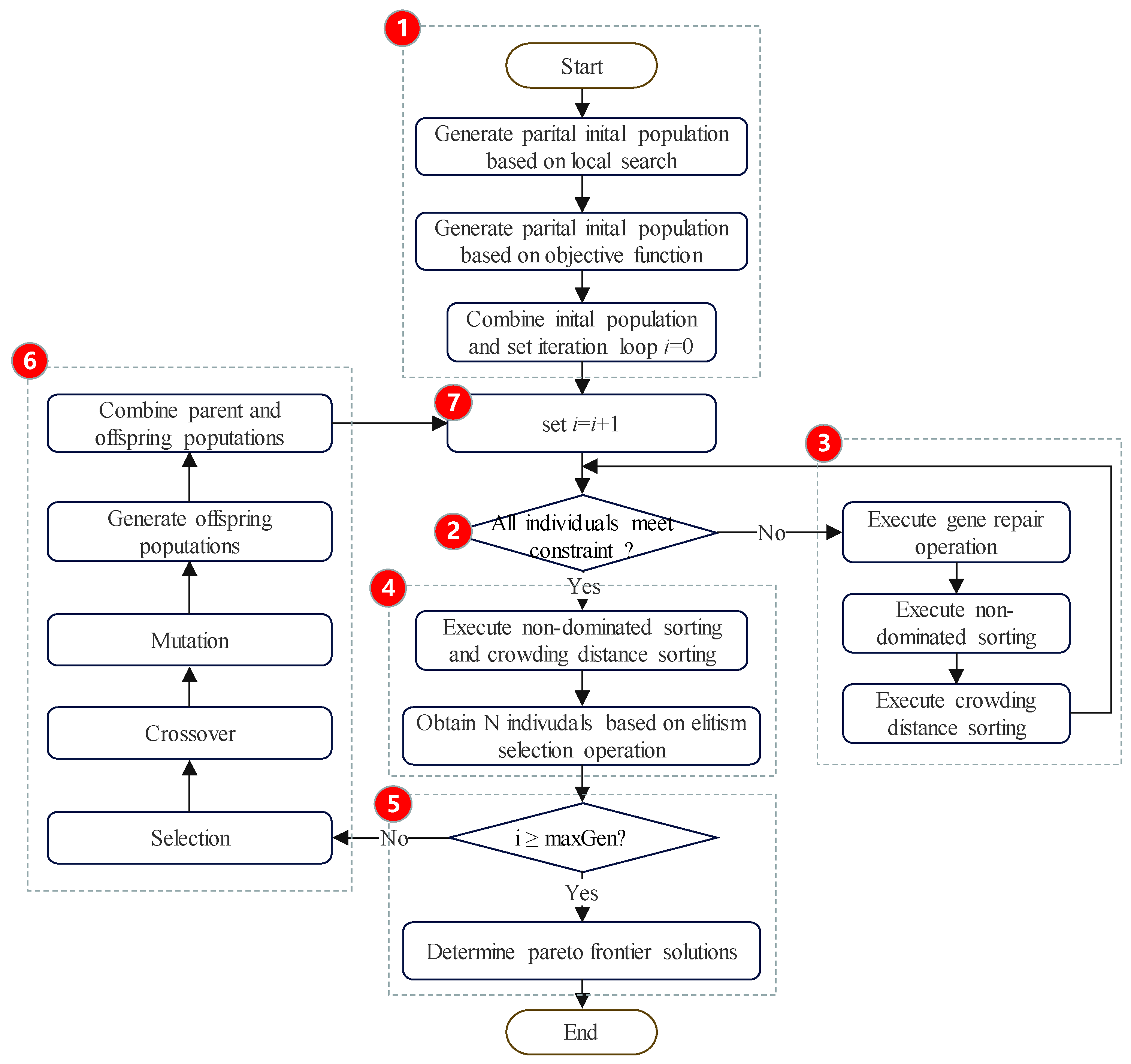
Task allocation and dynamic control have been addressed using various approaches. These methods include using a Markov decision process for decision-making, employing mixed integer nonlinear programming or genetic algorithm for optimization, and applying multi-objective optimization, such as Non-Dominated Sorting Genetic Algorithm-II (NSGA-II), to solve multiple objectives. The NSGA-II algorithm, which incorporates fast non-dominated sorting, crowding degree, and elite selection strategies, is known for its high speed and excellent convergence performance. It ensures the effectiveness in solving multi-objective optimization problems. To address the proposed model, this study improves the traditional NSGA-II algorithm by focusing on the chromosome repair and initial population generation operations, thereby forming the improved Non-Dominated Sorting Genetic Algorithm-II with Repair Mechanism (NSGA-II_RM) algorithm. The detailed algorithm flow is illustrated in Figure 5, and involves the following main steps:

Step 1: Set the population size to N, and generate the initial population by using a local search and an objective function based on the proposed improved initial solution generation operation. This population is referred to as the 0th generation population.

Step 2: Determine whether all individuals in the population meet the constraint conditions. If not, Step 3 is executed; otherwise, Step 4 is executed.

Step 3: The gene repair operation is executed on the chromosomes until all the constraints are met.

Step 4: The population is sorted by fast non-dominated and crowding distance. The N individuals are then selected based on an elite retention strategy and divided into set C.

Step 5: If the maximum number of iterations is exceeded, the final Pareto solutions set is determined; otherwise, Step 6 is executed.

Step 6: Select the parent chromosomes based on the tournament operation, generate N offspring chromosomes through uniform crossover and uniform mutation, and then merge the parent and offspring into the new population.

Step 7: Update the iteration number and go to Step 2.

In the above algorithm, the critical coding method, mutation operation, crossover operation, gene repair operation, and initial population generation operation are explicated as follows.

1.

Coding method

Considering that the material supply quantity of each supplier is an integer, an integer coding method is selected.

Assuming the required order consists of I material types, the chromosome is divided into I gene segments, denoted as O₁, O₂, ..., O_I. Each material type can be supplied by J_i suppliers, so segment O_i will consist of J_i genes. Each gene represents a specific allocated quantity, denoted as O_i1, O_i2, ..., $O_{i,J_i}$ where O_ij represents the decision variable x_ij.

2.

Crossover operation

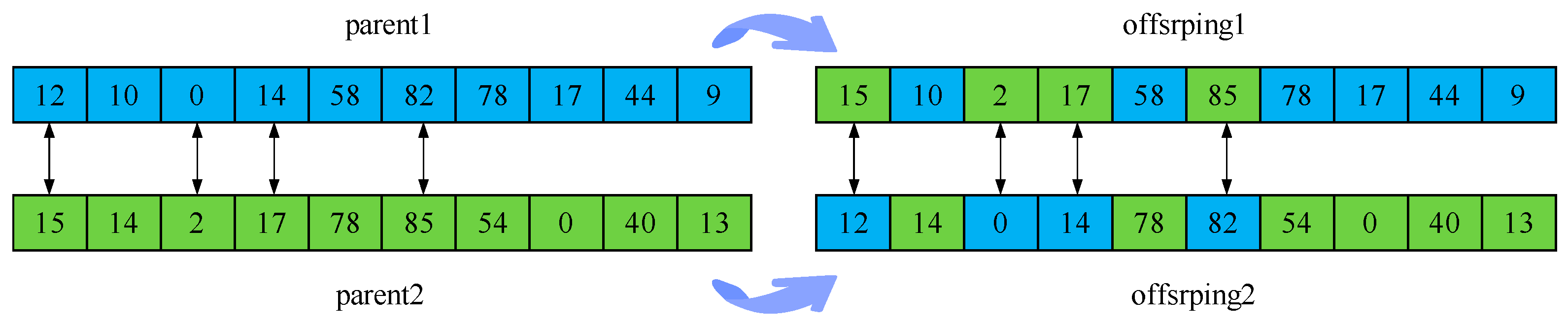
To improve the diversity of populations, the genes in the chromosomes are exchanged by uniform crossover, in which the genes at index i of two chromosomes are exchanged with crossover probability P_c. The specific operation process is shown in Figure 6, and the process is as follows:

(1) Traverse all gene loci from the two parent chromosomes sequentially.

(2) For each gene locus, the probability P is randomly generated. If P is less than or equal to P_c, the crossover operation is executed. During this process, the gene values of the two chromosomes at the index are exchanged; otherwise, they remain unchanged. After the crossover, the two offspring chromosomes are generated.

3.

Mutation operation

The uniform mutation method is similar to the above uniform crossover. In this method, it requires randomly changes the gene value on the individual chromosome. Each gene has the same chance of executing the mutation. The specific operation process is as follows:

(1) Traverse all genes sequentially and set the random probability P for each gene.

(2) For each point, the mutation probability P_m is used to judge whether the mutation occurs. If the P for each gene is less than or equal to P_m, the mutation will be carried out. During the process, a random integer value within the corresponding gene’s range is generated to replace its original value; otherwise, the original value is retained.

4.

Gene repair operation

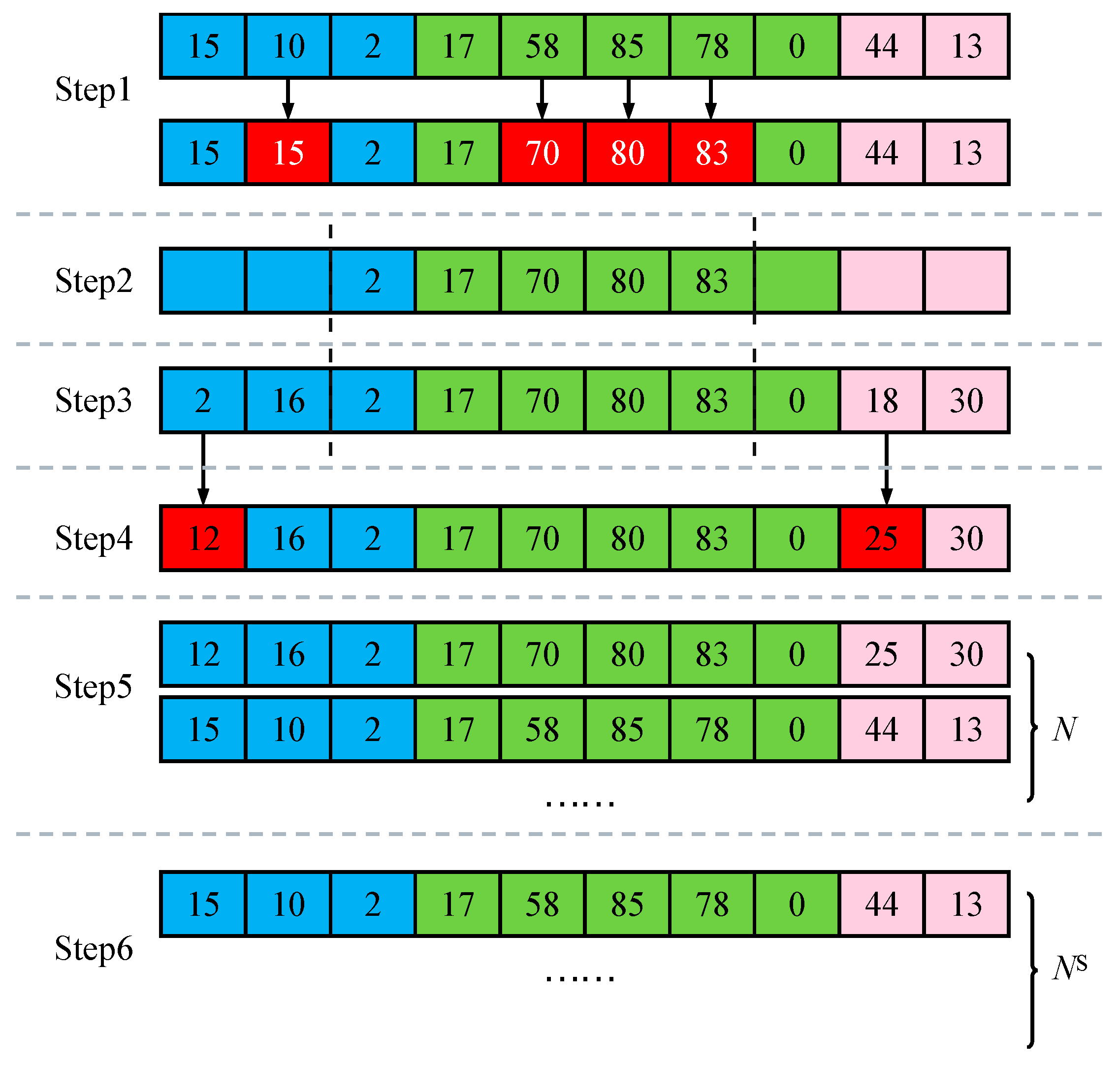
The offspring chromosomes resulting from the crossover and mutation operations are likely to fail to meet the constraint conditions. Therefore, the repeated mutation or crossover operation could be applied. However, when the constraints are complex and the gene scales are large, it is inefficient. To address this issue, this section introduces an improved gene repair mechanism to perform the operation. This mechanism converts infeasible solutions into feasible ones under constraint conditions, thereby avoiding the traditional repetitive operations and enhancing the overall performance. The specific process is as follows:

(1) Check and adjust the supply quantity of each supplier: when the supply quantity is less than the minimum order quantity, randomly judge whether to select the supplier. If yes, set it to the minimum order quantity; otherwise, set it to 0. When the supply quantity is greater than the maximum supply quantity, set it to the maximum supply quantity.

(2) Check whether the allocation scheme meets the constraints: if not, randomly select one of the material suppliers and modify the supply quantity subject to the constraints. If still not, continue to select another supplier until the conditions are met.

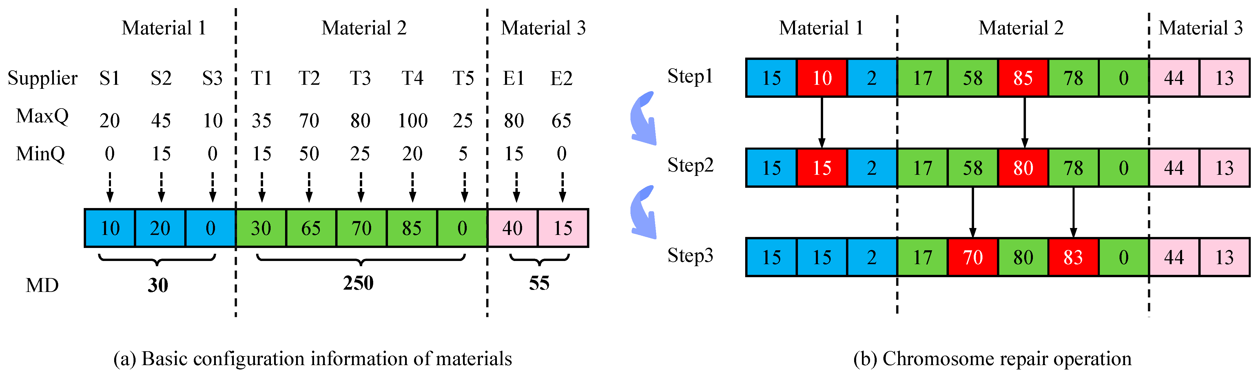
For example, consider a kitting order consisting of three material types, with the number of suppliers for each material type being three (S1–S3), five (T1–T5), and two (E1–E2), respectively. The minimum order quantity (MinQ), maximum supply quantity (MaxQ), and material demand (MD) are shown in Figure 7a. The chromosome formed after crossover and mutation is illustrated in Step 1 of Figure 7b. First, the genes on the chromosome are checked: the supply quantity (10) for the second gene is less than the minimum order quantity (15), and the supply quantity (85) for the sixth gene exceeds the maximum supply limit (80). Next, the incorrect genes are repaired: the supply quantity for the second gene is set to the minimum order quantity (15), and the supply quantity for the sixth gene is adjusted to the maximum supply limit (80). In this case, the total supply quantity (233) for the second material is below the total demand (250), which does not meet the demand constraint. Thus, suppliers for the materials are randomly selected, and the supply quantities for the fifth and seventh genes are adjusted to 70 and 83, respectively. The repair operation is performed.

5.

Initial population generation operation

A diverse and high-quality initial population can significantly enhance algorithm performance, thereby quickly obtaining the optimal solutions. In the NSGA-II algorithm, the conventional initial population is generated randomly. The genes for each chromosome are randomly assigned values until all the chromosomes meet the constraint conditions. This process is repeated and inefficient. Moreover, the order of reallocation is inclined to select the solutions that have minimal changes relative to the initial allocation schemes. To address these issues, this section introduces the improved population initialization method based on the local search and objective function, aiming to improve the population quality and enhance overall algorithm performance. Assuming the population size is N, the specific process is as follows.

(1) Initialization based on local search

Firstly, a local search operator is designed to search for the optimal initial solutions. The search process is shown in Figure 8. Concretely:

Step 1: Judge whether the initial allocation scheme meets the dynamic requirements or new constraints. If not, execute the repair operation to obtain the new chromosomes.

Step 2: Randomly retain some genes and remove the other genes on the chromosome.

Step 3: After the removal, the values on their corresponding genes are randomly generated subject to the boundary conditions.

Step 4: Judge whether the individual chromosome generated in Step 3 meets the whole constraint conditions. If not, a repair operation is executed to obtain the updated chromosome.

Step 5: Repeat Step 2, Step 3, and Step 4 until N chromosomes are generated.

Step 6: Perform a fast non-dominated sorting on the above N chromosomes and select the best N^S ones.

(2) Initialization based on objective functions

The proposed model involves multiple non-dominated optimization objectives. The boundary solution is characterized by being optimal for one objective while being worse for others. To leverage this characteristic, this section employs an initial population generation method based on the objective function. This approach ensures that the initial population is more widely distributed across the boundary of the true optimal solution set, thereby enhancing the diversity of solutions. The specific process is as follows:

Step 1: Determine the number n of objective functions.

Step 2: Aiming at the ith objective function, generate N chromosomes randomly as candidate solutions.

Step 3: Calculate the ith objective value of all candidate solutions, and sort them according to the preference of these values.

Step 4: Obtain $N_i^{\mathrm{O}}$ optimal solutions from the above ranking.

Step 5: Repeat Steps 2 to 4 to obtain multiple solution sets for the n objective functions.

In our paper, the reallocation model involves two objectives, thereby yielding $N_1^{\mathrm{O}}$ and $N_2^{\mathrm{O}}$ solution sets, respectively. Considering the equal value for the two optimization objectives, the $N_2^{\mathrm{O}}$ value is set to be equal to the $N_1^{\mathrm{O}}$ value_.

Overall, the N^S solutions from the local search aim to find more solutions that are closer to the initial allocation schemes, while the $N_1^{\mathrm{O}}$ and $N_2^{\mathrm{O}}$ solutions from the objective functions focus on enhancing the respective optimal objective. Moreover, to improve the algorithm’s diversity and avoid local situations, the $N^{\mathrm{R}}$ random solutions are also set. Therefore, their size proportions r_ini are determined by the following formula:

$$\left\{\begin{array}{c}N=N^{\mathrm{S}}+N_1^{\mathrm{O}}+N_2^{\mathrm{O}}+N^{\mathrm{R}}\\ r_{\mathrm{ini}}=\left[N^{\mathrm{S}},N_1^{\mathrm{O}},N_2^{\mathrm{O}},N^{\mathrm{R}}\right]=\left[0.2, 0.3, 0.3, 0.2\right]\end{array}\right.$$

(11)

6. Case Study

6.1. Case Description and Parameter Setting

Assume that a home appliance company, G,, includes 10 suppliers: S1 to S10. S1 to S2 supply evaporator components, S3 to S7 supply condenser components, and S8 to S10 supply compressor components. Company G completes the production of air conditioning products by purchasing and assembling these component materials. Specifically, in one production purchase, the initial material requirements are 1000 evaporators, 4500 condensers, and 1000 compressors. The initial kitting allocation plan scheme for S1–S10 in order is [37, 222, 287, 436, 527, 778, 948, 990, 1000, 1275].

At a certain time, due to the planning adjustments in order demand, the procurement quantities for evaporators, condensers, and compressors were changed to 900, 3600, and 900, respectively. The final order delivery time and other parameters are provided as shown in

Table 2. Model parameters.

Items	s1	s2	s3	s4	s5	s6	s7	s8	s9	s10
$x_{ij}^{\min }$	100	0	300	100	0	50	60	30	30	20
$x_{ij}^{\max }$	600	1000	1000	1200	1500	1400	1000	500	600	600
Qi	900		3600					900
$p_{ij}^{\mathrm{dq}}$	0.03	0.05	0.025	0.04	0.03	0.05	0.02	0.035	0.05	0.04
$p_{ij}^{\mathrm{de}}$	0.02	0.03	0.025	0.015	0.03	0.03	0.025	0.025	0.03	0.03
cr	90%
Dd	20
$t_{ij}^{\mathrm{p}}$	1/60	1/85	1/90	1/125	1/134	1/132	1/102	1/48	1/50	1/58
$D_{ij}^{\mathrm{t}}$	0.5	1.0	1.0	1.5	1.0	2.0	1.0	0.5	0.5	0.25
$l$	300
$c_{ij}^{\mathrm{b}}$	460	325	51	45	38	32	53	400	286	335
$c_{ij}^{\mathrm{f}}$	20	35	2	3	6	2	5	15	30	25

. Currently, it is necessary to adjust the allocation scheme (namely, the initial scheme) and dynamically determine the reallocation schemes to meet the following kitting requirements. The algorithm-related parameter is set, where population size is 200, the maximum number of iterations is 1000, mutation probability is 0.2, and crossover probability is 0.8.

6.2. Experiment Results

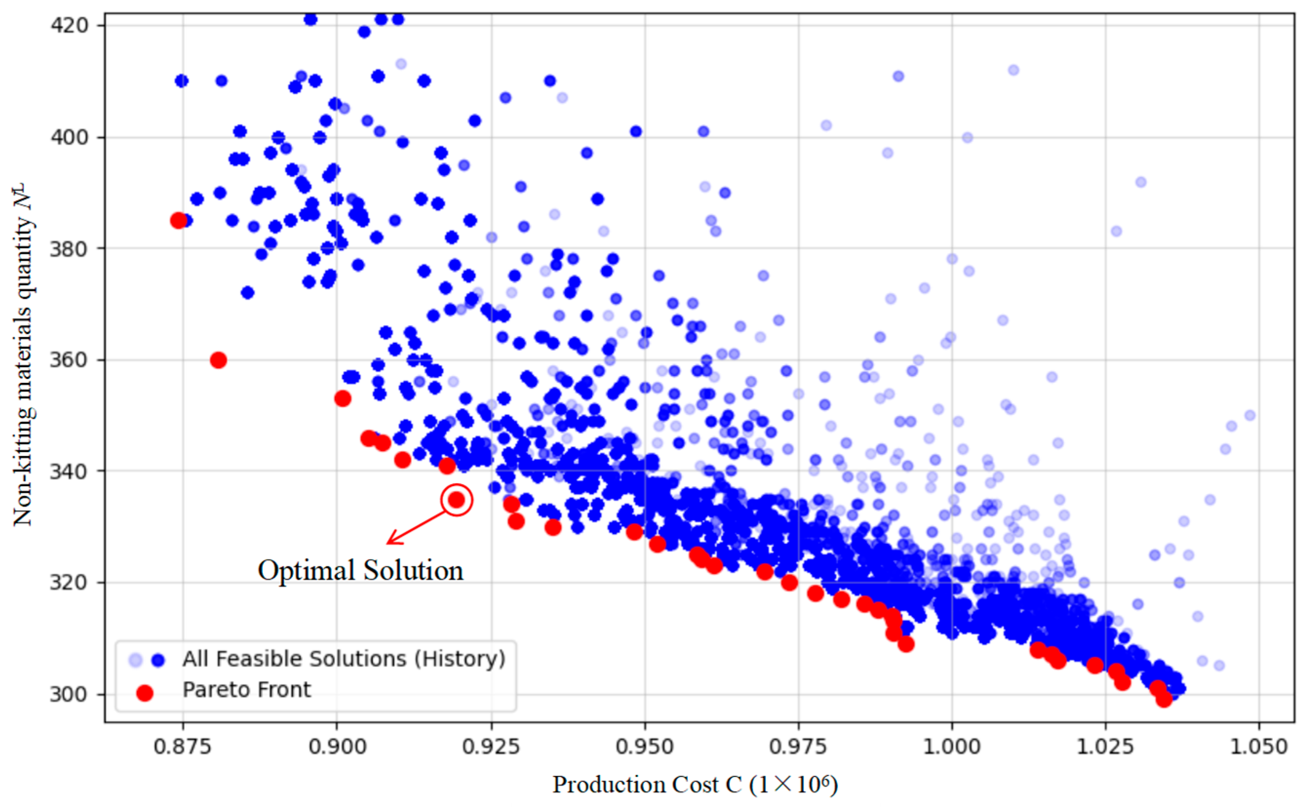
In view of the above case, the proposed NSGA_II_RM algorithm is used to solve the problem, and the final optimal Pareto solution set is shown in Figure 9.

In the above frontier solution set S_p, there are several feasible solutions.

Table 3. Feasible Pareto frontier solution set (partial).

No.	S1	S2	S3	S4	S5	S6	S7	S8	S9	S10	F1	F2	${\mathit{E}}_{{\mathit{P}}_{\mathit{i}}}$
1	0	965	1000	981	1273	624	0	0	498	459	874,270	385	1
2	0	965	1000	1200	1400	0	199	0	498	459	880,696	360	0.7494
3	0	943	1000	981	1273	0	420	0	498	459	900,940	353	0.7945
4	0	922	1000	1200	1400	0	0	0	591	325	905,130	346	0.7392
5	0	920	1000	1200	1400	0	0	0	522	396	907,392	345	0.7417
6	0	920	1000	1200	1166	0	234	0	522	396	910,668	342	0.7273
7	0	913	1000	1200	1029	0	371	0	591	325	917,902	341	0.7609
8	0	928	1000	1200	650	0	750	0	400	531	919,278	335	0.6997
9	0	911	1000	1200	588	0	818	0	514	396	928,244	334	0.744
...	...	...	...	...	...	...	...	...	...	...	...	...	...
32	600	300	1000	1200	400	0	1000	500	400	0	1,027,700	302	0.993
33	600	300	1000	1200	462	0	938	400	0	500	1,033,532	301	1.0178
34	600	300	1000	1200	400	0	1000	400	0	500	1,034,400	299	1

presents the partial solutions and their corresponding objective function values.

In order to determine the optimal scheme, the evaluation indicator is given as follows:

$$E_{P_i}={\displaystyle \sum _{k=1}^n\frac{f_{P_i}^k-f_{S_p}^{best,k}}{f_{S_p}^{worst,k}-f_{S_p}^{best,k}}}$$

(12)

where $E_{P_i}$ represents the evaluation value of individual chromosome P_i in the above Pareto solution set S_p, $f_{P_i}^k$ is the k-th objective value of P_i; $f_{S_p}^{best,k}$ and $f_{S_p}^{best,k}$ reveal the best and worst value of the k-th objective value of all individuals in S_p, and n is the number of objectives for an individual. Learning from the equation, it is known that the smaller the evaluation indicator is, the more outstanding the individual is.

Based on the above indicator, the evaluation results of all the solution sets are obtained. In this, the evaluation value of the 8th solution, as shown in Figure 9, is the smallest, namely 0.6997. The corresponding optimal dynamic reallocation scheme for S1–S10 is [0, 400, 531, 650, 750, 928, 1000, 1200]. In this case, the final allocated materials for evaporators, condensers, and compressors are 928, 3600, and 931, which meet the adjusted procurement quantities of 900, 3600, and 900. Moreover, in this solution, the production cost objective is C = 919,278 yuan, and the non-kitting materials quantity objective is N^L = 355. They are both relatively smaller.

6.3. Comparative Analysis

6.3.1. Effectiveness Analysis

To verify the effectiveness and superiority of the proposed method, this section compares the proposed method with the traditional NSGA-II method. The comparisons will be analyzed from three indicators: convergence, uniformity, and generality [31].

1.

Convergence

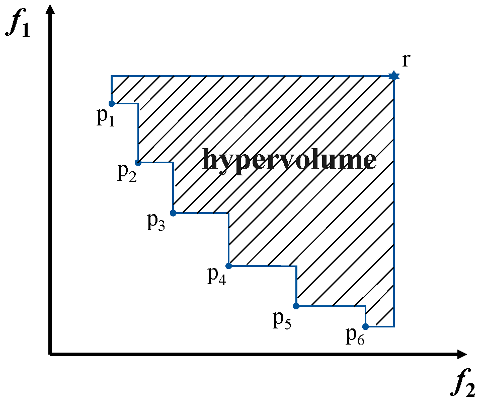
The hyper volume (HV) indicator is applied to reveal the convergence. In our paper, the meaning of hyper volume is shown in Figure 10.

In the figure, p_i represents the i-th solution in the frontier solution set, and r is an arbitrarily selected reference point. The calculation formula is as follows:

$$\mathrm{HV}=\delta \left({\cup }_{i=1}^{\left|S\right|}{v}_i\right)$$

(13)

where $\delta$ represents the Lebesgue measure, which is used to measure the volume, $\left|S\right|$ indicates the number of non-dominated solution sets, and v_i is the hyper volume formed by the reference point and the i-th solution in the solution set.

The HV can be calculated without a reference set or real frontier solution set, and the convergence and diversity of the solution set can be evaluated by the volume value in space. The larger the value is, the better the algorithm performance is.

2.

Uniformity

The diversity metric (DM) indicator is used to reveal the uniformity. The DM is formulated as:

$$\mathrm{DM}={\displaystyle \frac{d_f+d_l+{\displaystyle \sum _{i=1}^{N-1}\left|d_i-\overline{d}\right|}}{d_f+d_l+\left(N-1\right)\overline{d}}}$$

(14)

where d_f is the Euclidean distance between the lower bound solution and the lower extreme solution, d_l is the Euclidean distance between the upper bound solution and the upper extreme solution, d_i represents the Euclidean distance between the continuous solutions in the N solution set, and $\overline{d}$ indicates the average value of all the d_i.

For a non-dominating solution set, when the solution has the largest range, and the parameters d_f and d_l are regarded as 0, if the solution is in accord with the absolute average distribution, the d_i equals the $\overline{d}$, and thus the DM will be smaller. Therefore, the smaller the DM, the better the performance of the algorithm.

3.

Generality

The coverage metric (CM) indicator is applied to reveal the generality. It is calculated as follows:

$$\mathrm{CM}={\displaystyle \frac{\left|\left\{b\in \mathrm{B}\left|\exists a\in \mathrm{A}:a\succ b\right.\right\}\right|}{\left|\mathrm{B}\right|}}$$

(15)

where A and B represent two different solution sets, and a and b are the one solution in A and B.

In this formula, the numerator represents the total number of solutions in B that are dominated by solutions in A, and the denominator represents the total number of solutions in B. When this value is larger, it indicates that the more solutions in B are dominated by solutions in A, and obviously, the solution set of B is far worse than that of A.

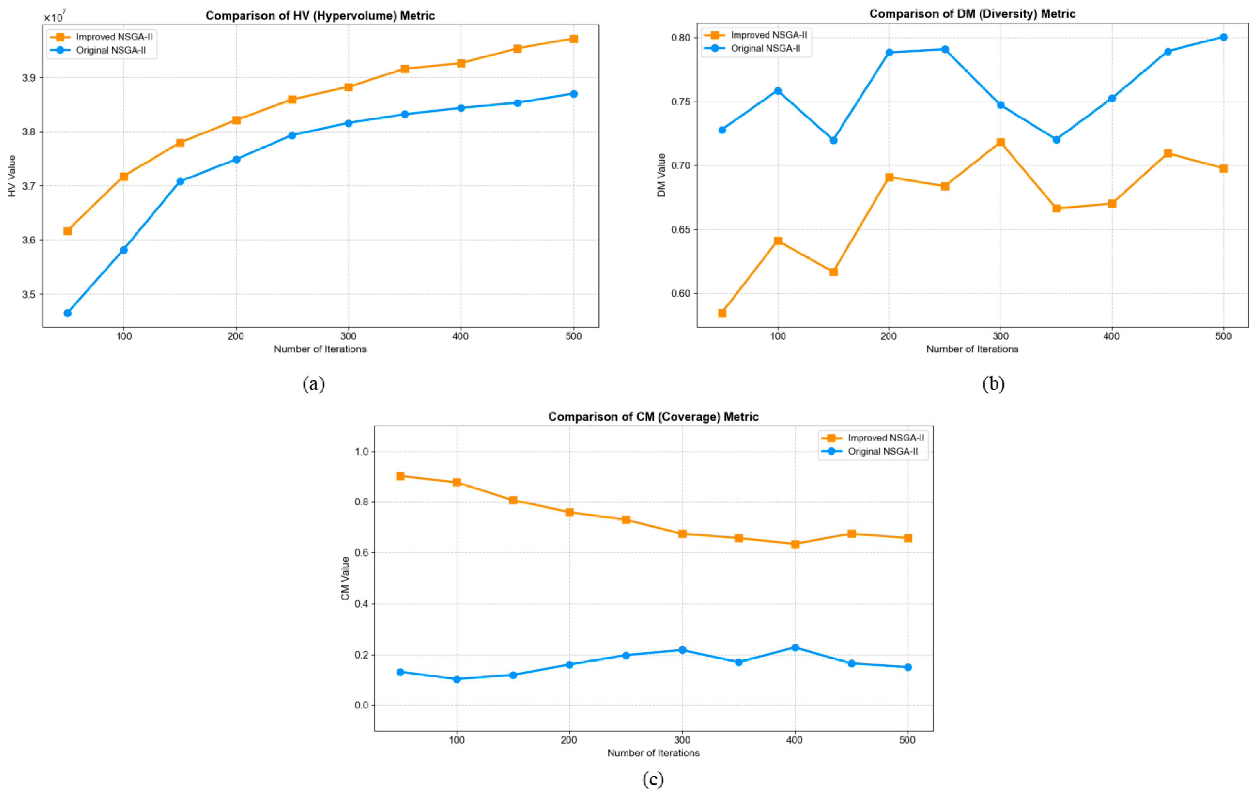
Based on the above indicators, this section selects the traditional NSGA-II and improved NSGA-II_RM algorithm to fulfill the comparative analysis. The algorithms are calculated repeatedly 10 times. The average calculation results for different numbers of iterations are shown in Figure 11.

Learning from the above results, it is revealed that:

• The HV value for the improved NSGA-II is greater than that of the traditional NSGA-II, and the average HV value before and after improvement is 3.754 × 10⁷ and 3.865 × 10⁷, respectively. The average HV value is increased by 2.96%, indicating that the convergence of the solution set is better than before improvement.
• The DM value for the improved NSGA-II is smaller than that of the traditional NSGA_II, and the average DM value before and after improvement is 0.7579 and 0.6698, respectively. The DM value is reduced by 11.63% on average, indicating that the final distribution range of the solution is wider, the uniformity is larger, and the algorithm performance is better.
• The CM reflects the quality and generality of solutions obtained, indicating the proportion of better solutions. In the tests, the CM value was 0.1642 before the improvement and 0.7378 after the improvement, indicating that the solutions in the improved algorithm are superior to those before the improvement. This reveals that the improved algorithm has achieved a more optimal solution set.

To sum up, the final solution set of the improved algorithm is better than that of the traditional algorithm in terms of convergence, distribution range, and diversity.

6.3.2. Sensitivity Analysis

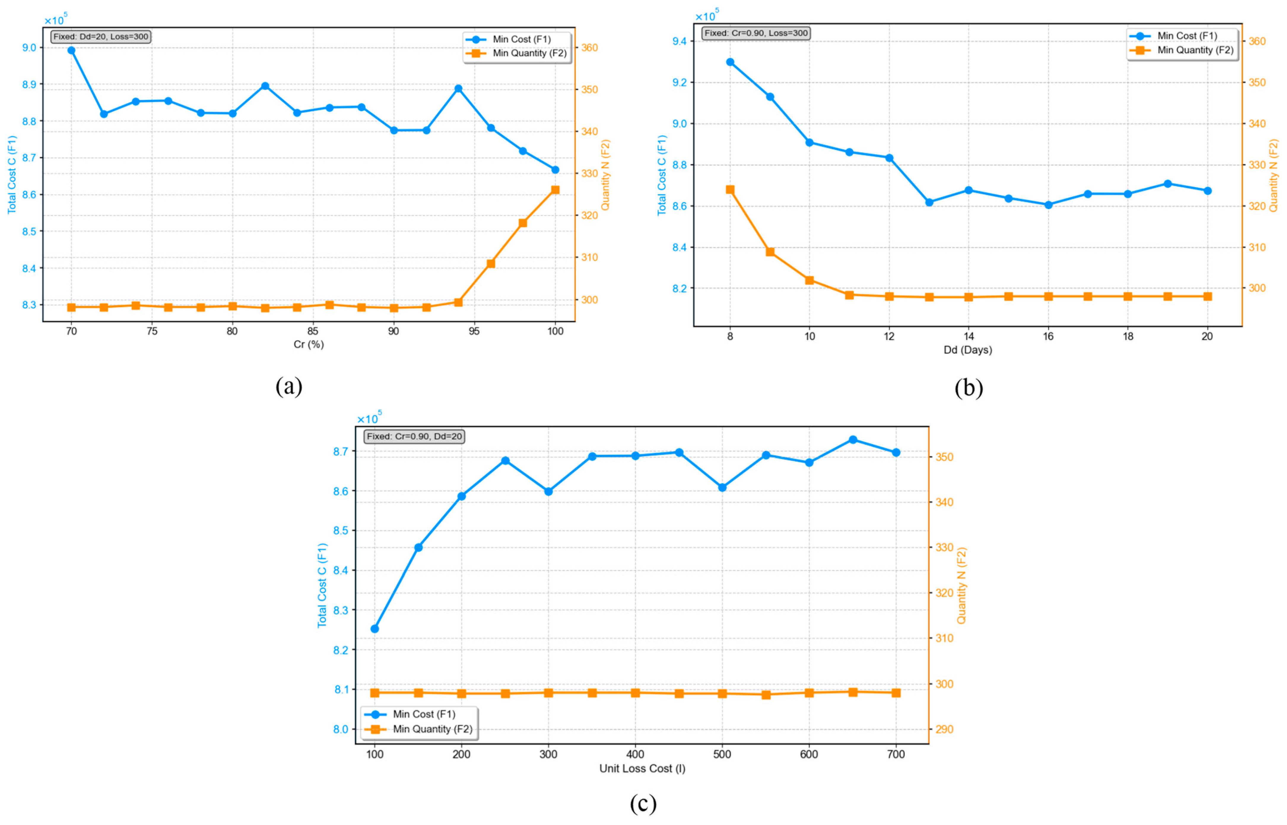
To verify the sensitivity of the proposed method on different parameters, this section compares the objective results from different values of kitting rate cr, order delivery time D^d, and loss cost per unit product l. The results are shown in Figure 12.

On the basis of the above result, it is known that:

• The kitting rate cr is sensitive to the two optimization objectives, especially when cr exceeds a certain threshold value 94%. When cr increases from 70% to 94%, the non-kitting N^L remains almost unchanged, fluctuating only within a very small range. For the minimum cost C, there is a slight downward trend and fluctuation, but the decrease amplitude is also minimal. However, when cr exceeds 94%, the N^L increases sharply, while the C decreases sharply. This indicates that when cr is lower than 94%, the proposed method could obtain the optimal kitting ability and minimum production cost. They are stable with respect to the lowest kitting rate limit. However, if cr is higher than 94%, the kitting ability cannot be maintained. In this, a larger quantity of material will be produced to meet kitting, and cheaper suppliers will be selected to decrease costs. Therefore, the N^L will increase, and C will decrease.
• The order delivery time D^d shows a high degree of sensitivity to both optimization objectives. As D^d increases from 8 days to 12 days, the minimum quality N^L of non-kitting materials decreases gradually. Specifically, when D^d is 8 days, N^L is 324; when D^d increases to 12 days, N^L drops to 299. The reduction rate between each interval is approximately 2%, showing a clear negative correlation. However, when D^d reaches the threshold value of 12 days, the minimum N^L will not decrease. Similarly, the total cost C shows a similar trend. When D^d increases to 13 days, the cost will not decrease. This reveals that when D^d is longer, the suppliers could have more time to fulfill the production, and thus, this leads to a small fluctuation beyond the threshold value.
• Regarding the loss cost l per unit product, this exhibits a significant sensitivity to the total cost C but has little impact on the quality N of non-kitting materials. When l increases from 100 yuan to 250 yuan, the minimum quality N^L remains stable at around 299. However, the minimum total cost C increases with the increase of l. For example, when l is 100 yuan, the minimum C is 825,306 yuan; when l is 150 yuan, C is 845,698 yuan, and when l is 250 yuan, C rises to 867,691 yuan. The average increase rate per 50-yuan rise in l goes from 2.47% to 1.30%, showing a positive but slower increase as l increases. When l reaches a certain threshold value, it will not increase. Meanwhile, the minimum quality N^L is not related to the loss cost l. This indicates that the kitting is not related to the loss cost l, which solely affects the material production costs. Moreover, to lower the minimum cost limit, it is necessary to strictly control the loss cost per unit product l within a reasonable range, especially when l is in the lower to medium range.

6.3.3. Simulation Analysis

Furthermore, to verify the performance of the proposed method on different suppliers or material sizes, this section compares the proposed method with traditional NSGA-II and simulation software Gurobi 10.0.0. The size is set as I/J_i, where I is the number of material types, and J_i is the matched number of suppliers for material M_i. For example, the “3/3” represents the size that includes 3 materials, and 3 suppliers for each material; while “3/r(2,10)” represents the size that includes 2 materials, and random 2–10 suppliers for each material. Note that the same sizes use the same initial parameters. The different sizes use different parameters generated randomly. The simulation results are shown in

Table 4. Simulation results for different supplier or material sizes.

Size	NSGA-II_RM			NSGA-II			Gurobi
	F1	F2	t/s	F1	F2	t/s	F1	F2	t/s
3/3	644,132	205	41	924,527	206	18	595,175	202	16
3/5	874,943	309	107	1,224,373	273	40	944,261	253	33
3/7	1,051,479	154	74	542,418	232	50	510,750	140	20
3/10	999,630	193	102	964,362	175	56	401,852	142	14
3/r(2,10)	1,158,006	230	101	1,156,628	245	56	875,260	255	10
5/3	1,661,380	449	48	1,572,250	414	75	1,276,035	391	31
5/5	2,024,307	636	43	1,944,781	621	73	1,505,256	394	41
5/7	2,066,489	569	96	1,825,412	495	24	973,893	274	43
5/10	3,402,091	628	88	3,870,196	794	35	1,248,637	367	93
5/r(2,10)	1,710,006	438	83	1,950,652	538	51	1,183,889	330	50
7/3	3,587,392	767	77	3,828,884	823	19	3,102,184	639	75
7/5	2,988,436	638	186	3,013,675	669	30	1,701,701	484	329
7/7	3,751,620	817	71	4,318,405	852	33	1,477,084	397	328
7/10	4,259,191	932	243	4,952,932	1102	196	1,856,413	380	271
7/r(2,10)	2,578,770	401	146	2,741,973	435	62	1,642,523	278	36
10/3	3,805,210	658	120	3,590,912	788	25	2,447,350	457	96
10/5	5,193,077	1175	114	5,487,549	1431	40	1,783,232	702	1599
10/7	6,955,199	1393	121	8,961,774	1873	43	2,811,444	679	676
10/10	7,267,960	1528	139	10,362,387	2087	31	1,668,977	473	1660
10/r(2,10)	3,885,793	1042	67	5,231,539	1176	23	1,977,202	592	1161
15/3	6,435,600	1512	251	7,124,414	1580	25	3,860,115	884	461
15/5	8,543,084	1777	124	9,007,945	2097	47	1,711,992	1329	1802
15/7	11,147,603	2366	138	13,769,695	3358	33	-	-	-
15/10	15,336,533	2918	142	16,865,887	3532	72	-	-	-
15/r(2,10)	7,402,195	2025	289	9,612,965	2252	75	3,300,747	914	1801

.

Learning from the above results, it is known that:

• Compared with the traditional NSGA-II, NSGA-II_RM demonstrates a significant advantage in solution quality. In nearly all test instances, especially in medium-to-large-scale problems such as “10/10”, “15/7”, and “15/10”, NSGA-II_RM achieves consistently better F1 and F2 values than the traditional NSGA-II. For example, in the 15/7 size, NSGA-II_RM obtains F1 = 11,147,603 and F2 = 2366, while NSGA-II yields F1 = 13,769,695 and F2 = 3358. These improvements reveal that the mechanisms introduced in NSGA-II_RM enable more effective exploration of the solution space, leading to a superior Pareto front approximation under the same computational resources.
• Compared with Gurobi, NSGA-II_RM offers superior solution speed and practical stability for large-scale problems. Although Gurobi can quickly obtain optimal solutions for small-scale instances, its computation time increases dramatically as the problem size grows. Especially, when I exceeds 7, and J_i exceeds 5, the average computation time will exceed 300 s. In contrast, NSGA-II_RM consistently obtains feasible solutions within a few hundred seconds (not exceeding 300 s) across all tested sizes, demonstrating much better time efficiency and robustness. Therefore, NSGA-II_RM is a more practical and reliable choice when the problem scale exceeds the capacity of exact solvers. However, it is noted that the solutions set is relatively worse in NSGA-II_RM, compared with the exact Gurobi methods.
• Overall, NSGA-II_RM exhibits a clear advantage in large-scale problem solving, offering the most balanced and robust performance. When the problem scale becomes too large for exact methods like Gurobi to handle, and when the traditional NSGA-II shows notable degradation in solution quality, NSGA-II_RM continues to stably produce high-quality feasible solutions for engineering applications. This achieves the best trade-off among solution quality, computational efficiency, and scalability, making it the preferred method for large-scale, complex multi-objective optimization problems, particularly those involving large supplier or material sizes.

6.4. Discussion

To verify the feasibility and effectiveness of the proposed method, this paper presents a real case study from a home appliance company G, and conducts comprehensive comparative analyses, including effectiveness analysis, sensitivity analysis, and simulation analysis.

In the case study, the proposed NSGA-II_RM algorithm was applied to optimize the kitting-oriented multi-objective order reallocation model. From this, company G could obtain a dynamic optimal kitting reallocation scheme, namely [0, 928, 1000, 1200, 650, 0, 750,0, 400, 531], which is adjusted from the initial allocation scheme [222, 778, 948, 990, 1275, 287, 1000, 37, 527, 436] due to planning adjustments. The obtained reallocation scheme not only meets the adjusted quantities 900, 3600, and 900 for three materials, but also achieves an optimal balance between cost and kitting objectives. The feasibility is validated in real-world scenarios.

In the effectiveness analysis, three indicators, including hyper volume (HV), diversity metric (DM), and coverage metric (CM), are used to reveal the convergence, uniformity, and generality of the proposed NSGA-II_RM method. Compared with traditional NSGA-II, the improved indicator results demonstrate the superior performance of NSGA-II_RM. It also exhibits the advantages of the designed chromosome repair mechanism and initial population generation operations. The repair operation ensures that generated solutions are feasible, avoids repetitive operations, and enhances the overall performance. The initial population generation operations merge the initial allocation scheme, boundary optimal solutions, and necessary random solutions, which enhances the convergence and generalization. This verifies the novelty and effectiveness of the proposed improvement to NSGA-II.

In the sensitivity analysis, the key parameters of the proposed order reallocation model were systematically investigated. They include kitting rate cr, order delivery time D^d, and loss cost per unit product l. Based on the sensitivity results, it is observed that D^d is highly sensitive to cost and kitting objectives below a certain threshold; l is sensitive to cost; and cr is sensitive to both objectives beyond a certain threshold. When D^d is less than 12 days, both the minimum cost and kitting quantity will be increased. The limited remaining time is insufficient to fulfill production adjustments. Therefore, it is necessary to avoid order reallocation operations when the remaining delivery time is less than 12 days. When l is less than 250 yuan, the cost increases as l increases. Therefore, to reduce reallocation cost, l should be strictly controlled by various methods, especially when it is small. For cr, the results show that the model could obtain optimal kitting and cost when the kitting rate limit is less than 94%. If the decision maker aims to reduce the minimum cost, cr can be increased. However, in this case, the non-kitting material quantity increases. Overall, the sensitivity results verify the advantage of the model and provide necessary adjustment advice regarding the reallocation process.

In the simulation analysis, the case data are extended to different scales with varying numbers of suppliers and materials, thereby verifying the effectiveness of the proposed method. This indicates that the proposed NSGA-II_RM could solve large-scale kitting-oriented order reallocation problems in a supply chain network with low computational time. It achieves a trade-off among solution quality, computational efficiency, and scalability, and can be applied to actual engineering problems. The practicability and effectiveness are both verified.

Overall, the proposed model and solution algorithm are both feasible and effective in solving the order reallocation and kitting problem. The kitting and reallocation are both integrated to implement dynamic adjustment with respect to the initial allocation scheme.

7. Conclusions

This paper addresses the critical challenge of achieving supply chain sustainability in large-scale manufacturing industries by proposing a novel kitting-oriented collaborative order reallocation method. The contributions are as follows:

• A large-scale collaborative production mode is proposed. Under this mode, a kitting-oriented dynamic collaborative control framework that integrates order reallocation operations is built. This framework provides systematic support for dynamic collaboration, integrating order kitting and order reallocation.
• Based on the initial order allocation scheme and dynamic disturbance information, a kitting-oriented order reallocation model is proposed. This considers sustainable kitting objectives and kitting constraints across multiple collaborative supplier enterprises. Moreover, an improved NSGA-II_RM algorithm is designed with novel chromosome repair operation and initial population generation operation. This contributes to obtaining the optimal reallocation scheme to adapt to the dynamic and kitting requirements relative to the initial scheme.
• The actual case study in the home appliance industry demonstrates the feasibility of the proposed method. The comparative analysis, involving effectiveness analysis, sensitivity analysis, and simulation analysis, verifies effectiveness from different perspectives. They reveal that the proposed method could obtain optimal reallocation results considering both kitting and cost objectives, while achieving a trade-off among solution quality, computational efficiency, and scalability. This could be applied to practical engineering problems.

In the future, the multi-layer kitting and order reallocation problem will be studied within the multi-layer supply network, thereby realizing effective multi-layer control and management for enterprise groups.

References

1. Chang, F.; Zhou, G.; Chang, F.; Ding, K.; Zhang, C.; Cheng, W. Original equipment manufacturer-dominated multi-player intelligent collaborative maintenance service mode. Comput. Integr. Manuf. Syst. 2023, 29, 1082–1096. [Google Scholar] [CrossRef]
2. Hong, Z.; Qu, T.; Zhang, Y.; Zhang, Z.; Huang, G.Q. Cloud-fog-edge based computing architechture and a hierarchical decision approach for distributed synchronized manufacturing systems. Adv. Eng. Inform. 2025, 65, 103386. [Google Scholar] [CrossRef] [Scilit]
3. Zhang, Z.; Qu, T.; Huang, G.Q.; Zhang, Y.; Zhao, K.; Zhang, J. Towards a trusted synchronized decision-making method for social production logistics systems based on blockchain and digital twin. Robot. Comput. Integr. Manuf. 2025, 94, 102965. [Google Scholar] [CrossRef] [Scilit]
4. Huan, A. Case study on supply chain financing of gree electric appliances. Inf. Syst. Econ. 2024, 5, 164–169. [Google Scholar] [CrossRef] [Scilit]
5. Zhang, H. The application of digital technology in tesla automobile industry: Key factors and global market expansion. Highlights Bus. Econ. Manag. 2023, 23, 1094–1098. [Google Scholar] [CrossRef] [Scilit]
6. Ronen, B. The complete kit concept. Int. J. Prod. Res. 1992, 30, 2457–2466. [Google Scholar] [CrossRef] [Scilit]
7. Çağlayan, M.S.; Aksoy, A. Integrating machine learning and material feeding systems for competitive advantage in manufacturing. Appl. Sci. 2025, 15, 980. [Google Scholar] [CrossRef] [Scilit]
8. Wang, W.; Wang, Y. Research and implement for kit-manufacturing model. Comput. Integr. Manuf. Syst. 2013, 19, 2795–2801. [Google Scholar] [CrossRef]
9. Montoya-Zapata, S.; Klement, N.; Silva, C.; Gibaru, O.; Lafou, M. Multi-agent system for perturbations in the kitting process of an automotive assembly line. Eng. Appl. Artif. Intell. 2024, 135, 108679. [Google Scholar] [CrossRef] [Scilit]
10. Fatima, U.; Mohammed, D.; Shareef, I. A holistic approach to kitting cart optimization and steel receiving analysis for process improvement. Manuf. Lett. 2024, 41, 1716–1727. [Google Scholar] [CrossRef] [Scilit]
11. Pan, Y.; Zhong, R.Y.; Qu, T.; Ding, L.; Zhang, J. Multi-level digital twin-driven kitting-synchronized optimization for production logistics system. Int. J. Prod. Econ. 2024, 271, 109176. [Google Scholar] [CrossRef] [Scilit]
12. Ostermeier, F.F.; Jaehnert, J.; Deuse, J. Joint modelling of the order-dependent parts supply strategies sequencing, kitting and batch supply for assembly lines: Insights from industrial practice. Prod. Manuf. Res. 2023, 11, 2200808. [Google Scholar] [CrossRef] [Scilit]
13. Bo, H.; Han, P.; Lu, B.; Zhao, C.; Wang, X. Online monitoring and collaborative scheduling method for wheelset cyber-physical production system: A wheelset manufacturing system case study from a Chinese high-speed train enterprise. Adv. Eng. Inform. 2021, 47, 101210. [Google Scholar] [CrossRef] [Scilit]
14. Najafi, M.; Zolfagharinia, H.; Rostami, S.; Rafiee, M. Enhancing supply chain resilience facing partial and complete disruptions: The application in the cooking oil industry. Appl. Math. Model. 2024, 131, 253–287. [Google Scholar] [CrossRef] [Scilit]
15. Pajic, V.; Andrejic, M.; Kilibarda, M. Procurement optimization by selecting efficient suppliers using dea-fucom-cocoso approach and solving order allocation problem. Facta Univ. Ser. Mech. Eng. 2025, 23, 109–125. [Google Scholar] [CrossRef] [Scilit]
16. Di Pasquale, V.; Nenni, M.E.; Riemma, S. Order allocation in purchasing management: A review of state-of-the-art studies from a supply chain perspective. Int. J. Prod. Res. 2020, 58, 4741–4766. [Google Scholar] [CrossRef] [Scilit]
17. Nguyen, T.; Amin, S.H.; Shah, B. A perspective on supplier selection and order allocation: Literature review. Adm. Sci. 2024, 14, 206. [Google Scholar] [CrossRef] [Scilit]
18. Zhang, J.; Wang, S.; He, W.; Li, J.; Cao, Z.; Wei, B.; Wang, M. Material kitting in selective assembly: A manual order picking system based on augmented reality. Int. J. Adv. Manuf. Technol. 2022, 123, 675–686. [Google Scholar] [CrossRef] [Scilit]
19. Zhu, H.; Fu, T.; Li, F.; Liu, C.; Cai, Q.; Tang, D. Prediction of process-level kitting time of assembly materials for complex products based on digital twin. J. Mech. Eng. 2025, 61, 384–398. [Google Scholar] [CrossRef] [Scilit]
20. Simoes, M.J.; Pinto, T.; Silva, C. Innovative hybrid kitting systems for automotive manufacturing: Performance analysis and optimisation. Int. J. Prod. Res. 2025, 63, 7013–7038. [Google Scholar] [CrossRef] [Scilit]
21. Khoshfetrat, S.; Rahiminezhad, G.M.; Almasi, M. Sustainable supplier selection and order allocation: A fuzzy approach. Eng. Optim. 2019, 52, 1494–1507. [Google Scholar] [CrossRef] [Scilit]
22. Vaezi, A.; Rabbani, E.; Yazdian, S.A. Blockchain-integrated sustainable supplier selection and order allocation: A hybrid BWM-MULTIMOORA and bi-objective programming approach. J. Clean. Prod. 2024, 444, 141216. [Google Scholar] [CrossRef] [Scilit]
23. Chen, X.H.; He, Y.; Pakdel, G.H.; Liu, X.F.; Wang, S. A comprehensive multi-stage decision-making model for supplier selection and order allocation approach in the digital economy. Adv. Eng. Inform. 2025, 63, 102961. [Google Scholar] [CrossRef] [Scilit]
24. Xu, H.; Liu, X.; Huang, H. Information sharing and order allocation rule in dual-sourcing. Omega 2023, 114, 102741. [Google Scholar] [CrossRef] [Scilit]
25. Alejo-Reyes, A.; Mendoza, A.; Olivares-Benitez, E. A heuristic method for the supplier selection and order quantity allocation problem. Appl. Math. Model. 2021, 90, 1130–1142. [Google Scholar] [CrossRef] [Scilit]
26. Li, F.; Wu, C.; Zhou, L.; Xu, G.; Liu, Y.; Tsai, S. A model integrating environmental concerns and supply risks for dynamic sustainable supplier selection and order allocation. Soft Comput. 2020, 25, 535–549. [Google Scholar] [CrossRef] [Scilit]
27. Nazari-Shirkouhi, S.; Miralizadeh Jalalat, S.; Sangari, M.S.; Sepehri, A.; Vandchali, H.R. A robust-fuzzy multi-objective optimization approach for a supplier selection and order allocation problem: Improving sustainability under uncertainty. Comput. Ind. Eng. 2023, 186, 109757. [Google Scholar] [CrossRef] [Scilit]
28. Islam, S.; Amin, S.H.; Wardley, L.J. A supplier selection & order allocation planning framework by integrating deep learning, principal component analysis, and optimization techniques. Expert Syst. Appl. 2024, 235, 121121. [Google Scholar] [CrossRef] [Scilit]
29. Tajally, A.; Babakhani, B.; Jeyzanibrahimzade, E.; Parvin, M.; Irani, S. Sustainable supplier selection and order allocation problem considering the agility and resilience dimensions: A novel multi-stage data-driven decision-making approach. Int. J. Syst. Sci. Oper. Logist. 2025, 12, 2458756. [Google Scholar] [CrossRef] [Scilit]
30. Gabellini, M.; Mak, S.; Schoepf, S.; Brintrup, A.; Regattieri, A. A continuous training approach for risk informed supplier selection and order allocation. Prod. Manuf. Res. 2024, 13, 2447035. [Google Scholar] [CrossRef] [Scilit]
31. Shi, M.; Zhu, J. Procurement optimization for manufacturing enterprises considering supply chain disruption risks and carbon emissions. Sustainability 2025, 17, 3532. [Google Scholar] [CrossRef] [Scilit]
Figure 1. Changes in the supply chain mode of the enterprise group.
Sustainability 18 04537 g001
Figure 2. Large-scale collaborative production mode (The colors represent the enterprise nodes in different layers).
Sustainability 18 04537 g002
Figure 3. Collaborative production process.
Sustainability 18 04537 g003
Figure 4. Dynamic collaborative control framework of enterprise group.
Sustainability 18 04537 g004
Figure 5. The algorithm flow of NSGA-II_RM (The numbers represent the key steps).
Sustainability 18 04537 g005
Figure 6. Crossover operation.
Sustainability 18 04537 g006
Figure 7. Chromosome repair operation.
Sustainability 18 04537 g007
Figure 8. Population generation based on local search.
Sustainability 18 04537 g008
Figure 9. The Pareto solution set of NSGA-II_RM.
Sustainability 18 04537 g009
Figure 10. Schematic diagram of super volume.
Sustainability 18 04537 g010
Figure 11. Result comparison of algorithms before and after improvement. (a) comparison of HV; (b) comparsion of DM; (c) comparsion of CM.
Sustainability 18 04537 g011
Figure 12. Sensitivity results on different parameter values. (a) kitting rate cr; (b) order delivery time Dd; (c) loss cost per unit product l.
Sustainability 18 04537 g012