Forecasting Peruvian Blueberry Exports for Sustainable Agricultural Trade Management: Markov Chains, SARIMA, and Log-Linear Growth

Abstract

Peruvian fresh blueberry exports have expanded rapidly since 2012, yet strong seasonality and price–volume fluctuations continue to complicate trade planning and export decision-making, thereby threatening the long-term economic sustainability of the sector. Using monthly series for 2012–2025, this study compares three forecasting approaches to export value (FOB), export volume and unit price: (i) a seasonal Markov chain with Monte Carlo simulation (Markov–Monte Carlo), (ii) a log-linear growth model, and (iii) a seasonal ARIMA (SARIMA) model estimated using logarithmic data. The models are evaluated under a common train–test design, with the last 12 months (September 2024–August 2025) reserved for out-of-sample assessment. Model performance was evaluated through standard metrics, specifically Mean Absolute Error (MAE) and Root Mean Square Error (RMSE), while model adequacy was examined through residual diagnostics, including Ljung–Box tests. For the Markov–Monte Carlo approach, simulated distributions were also used to characterize forecast uncertainty. Findings indicate that the log-linear growth model provides the most accurate short-term point forecasts for FOB values, and the SARIMA model performs better for export volume; the Markov–Monte Carlo approach, however, yields the best performance for export prices and provides additional insights into seasonal regimes. Overall, these results suggest that no single model dominates across all dimensions of the export chain. Instead, the combined use of forecast approaches offers a more comprehensive basis for sustainable trade management, export planning, and risk management in dynamic agricultural export sectors.

1. Introduction

1.1. Background and Motivation

Global agricultural markets have become increasingly influenced by geopolitical tensions, post-pandemic disruptions, and climate-related shocks. The COVID-19 crisis and the Russia–Ukraine war, which intensified in 2022, generated significant volatility in international trade flows and price levels, with some commodities experiencing price increases above 50% [1,2,3]. Under such conditions, export trajectories are rarely linear or homogeneous, while FOB values and exported volumes may expand rapidly, unit prices decline in response to intensified competition, supply expansion, and changes in cost structures.

Agricultural commodities are structurally exposed to fluctuations in production cycles, international prices, exchange rates, logistics constraints, and trade policy adjustments. These dynamics are especially pronounced in emerging export industries characterized by accelerated growth followed by phases of market adjustment and intensifying global competition [4,5]. Nonetheless, agricultural trade systems may also display heterogeneous resilience under external shocks, depending on product structure and market conditions [6,7].

The Peruvian fresh blueberry sector illustrates this trajectory [8], it accompanied by a significant expansion in the European Union and U.S. market [9]. Since 2012, Peru has evolved from a marginal exporter to the world’s leading supplier, with export values exceeding USD 2 billion in recent years and a significant share of global markets [10]. However, this expansion has been accompanied by episodes of marked volatility, such as the 2023 campaign, when reduced global output constrained volumes but elevated prices, generating sharp variations in total FOB value [11].

For exporters and policymakers, the interaction between strong seasonality, structural transformation, and price–volume dynamics complicates strategic planning. Decisions related to harvest scheduling, logistics contracting, pricing strategies, and risk management require forecasting tools capable of capturing both trend persistence and potential regime changes [12,13].

In practice, producers, trade associations, and managers often rely on relatively simple tools, such as average growth extrapolations, short-window linear projections, or basic comparisons across previous seasons. Although improved knowledge of export performance helps reduce losses and enhance success prospects [14], many empirical analyses still depend on correlation-based approaches grounded in a linear view of the data. These methods tend to replicate the same linear logic when generating forecasts, which conflicts with the evolving requirements of export market orientation—EMO [15]. In such contexts, linear projections often fail to adequately capture abrupt shifts in export volumes and unit prices, particularly in highly seasonal and rapidly expanding agricultural sectors.

While such approaches provide an initial approximation to long-term trajectories, they are poorly suited to capturing shock episodes—such as the 2023/24 campaign, or structural shifts in export markets. This mismatch between the complexity of export dynamics and the simplicity of commonly used tools underscores the need to evaluate richer, yet tractable, forecasting frameworks capable of representing temporal dynamics and quantifying uncertainty over one- to two-year horizons.

So, this study compares three forecasting approaches using monthly data for 2012–2025 and a common train–test design in levels and logarithmic scales.

1.2. Forecasting Approaches in Export Analysis

Forecasting approaches in international trade and agri-food markets can be grouped into three methodological categories. In applied forecasting, these include autoregressive time-series models, deterministic growth specifications, and regime-based frameworks, each designed to capture different aspects of temporal dynamics [16].

Autoregressive models are used to represent persistence and seasonal structures in monthly export series. Deterministic growth models, including semi-logarithmic specifications and compound annual growth rate estimators, provide interpretable measures of long-term expansion trends but may be less flexible under changing growth regimes. Regime-based approaches, including Markov chains, allow export performance to evolve across discrete states rather than along a single continuous trajectory.

Although each approach captures distinct dimensions of export dynamics, systematic comparative assessments across value, volume, and unit price within a single agricultural export chain remain limited.

1.3. Research Gap and Research Questions

The literature on time series forecasting in agriculture and international trade has relied predominantly on univariate models such as ARIMA and SARIMA. These models have been widely applied to the forecasting of food prices, agricultural commodities, and specific export series, showing good performance in capturing trend and seasonality [17]. However, many of these studies focus on a single variable, as the domestic price of a crop, and adopt a single methodological approach, without systematically comparing their performance against alternative models.

Recent empirical research on agricultural exports, especially from 2024 onwards, has relied on semilogarithmic specifications and compound annual growth rates (CAGR) to analyze long-term growth patterns and their stability. In several applications, these growth measures are combined with indicators of revealed comparative advantage to assess export potential in selected agricultural commodities [18,19]. Although these models are intuitive and transparent, they tend to summarize dynamics into a single average growth rate, which limits their ability to capture policy changes, external shocks, or episodes of high volatility.

In parallel, models based on Markov chains have gained prominence as tools for analyzing market share dynamics, trade direction, and persistence in destination markets through nonlinear representations of export behavior [20,21,22]. Additional applied studies further confirm the usefulness of Markov chain approaches for analyzing stability and destination dynamics in agricultural export markets [23]. Applications to marine products, fresh onions, coconut, and other agricultural commodities employ transition matrices to study changes in importer-country shares and to evaluate the stability of trade flows over time [24,25,26]. Some contributions further combine Markov approaches with growth and competitiveness measures to identify winning and losing markets [27]. Nevertheless, the explicit use of Markov chains as quantitative forecasting tools, combined with Monte Carlo simulations and directly compared with ARIMA/SARIMA and log-linear growth models, remains scarce in the literature on agricultural and food products.

Accordingly, a specific research gap can be identified. There is still limited empirical evidence that jointly compares the performance of (i) a Markov–Monte Carlo model, (ii) a log-linear growth model, and (iii) a seasonal SARIMA model, when these approaches are simultaneously applied to three dimensions of the same export value chain, FOB value, export volume, and unit price, and evaluated under homogeneous criteria of forecast accuracy and residual diagnostics. This gap is relevant for emerging economies with dynamic agricultural export industries, e.g., Peru’s blueberry industry.

Based on this gap, the present study addresses the following research questions: (i) Which forecasting approach is more reliable and exhibits lower short-term (12-month) forecast errors? (ii) To what extent do the results differ when the series are modeled in levels versus logarithmic scale, and what are the implications for business and policy decision-making? (iii) Do models that exhibit lower forecast errors also display better residual properties and greater robustness? These research questions guide the design of the study and frame the comparison of results across the different modeling and forecasting approaches applied to the case of Peruvian fresh blueberry exports.

1.4. Contributions and Structure of the Study

This research offers complementary insights into modeling and forecasting approaches for agricultural products. First, it proposes an integrated comparative framework that evaluates three forecasting methods, in particular a Markov–Monte Carlo model, a log-linear growth model, and a seasonal SARIMA model, applied to the same agro-export value chain in an emerging economy.

Second, the study jointly analyzes three dimensions of export performance: FOB value, export volume, and unit price, it makes possible to assess the robustness of conclusions regarding the best-performing model when shifting from one variable to another. In addition, both level specifications (millions of USD or kilograms) and logarithmic transformations are considered, allowing an evaluation of how scale affects forecast accuracy and residual stability.

Third, the analysis combines standard forecast error metrics (MAE and RMSE) with a detailed examination of residual behavior and statistical robustness. This includes residual autocorrelation tests using the Ljung–Box statistic, inspection of ACF and PACF patterns, and comparisons of residual dispersion and distributional shape across models. Furthermore, the Markov–Monte Carlo framework enables the derivation of risk-related measures based on the simulated distribution of outcomes (e.g., 5th and 95th percentiles), augmenting the evaluation capacity of the scenario and risk management process.

Finally, from an applied perspective, the search offers practical implications for agricultural export companies and policymakers, by identifying which forecasting approaches are more accurate and robust across different contexts (value, volume, and unit price; level versus logarithmic scale). These findings can inform decision-making related to crop planning, contract negotiation, logistics capacity planning, and the design of risk management instruments.

The remainder of the paper is organized as follows: Section 2 describes the methodology, including the construction of states and transition matrices for the Markov chain, the implementation of the Markov–Monte Carlo model, the specification of the log-linear growth model, and the estimation of SARIMA models, as well as the forecast evaluation metrics and residual diagnostics. Section 3 reports the empirical results, comparing model performance in level and logarithmic specifications for FOB value, export volume, and unit price. Section 4 discusses these findings in light of the existing literature and the implications for management and policy. Finally, Section 5 presents the conclusions, the main limitations of the study, and directions for future research.

1.5. Literature Review

1.5.1. Markov Chains and Stochastic Processes in Applied Research

Markov chains have been increasingly used across different disciplines to model stochastic processes that evolve over time. In the field of health sciences, for example, Ocaña-Riola shows that homogeneous Markov chains are more suitable than non-homogeneous ones for describing clinical trajectories and evaluating transitions between states, reinforcing their usefulness as a discrete-time modeling tool [28].

In management and administrative sciences, stochastic processes and Markov chains allow the representation of a variable that moves across mutually exclusive states, under the assumption that transition probabilities depend solely on the current state and not on the past trajectory [29]. This approach facilitates the analysis of system stability or instability by examining both the probability of remaining in a given state and the probability of transitioning to another.

More recently, Jiménez proposed a spatial Markov chain model for population growth, comparing its performance with four other statistical forecasting tools [30]. His study highlights two aspects that are particularly relevant for the present research: (i) the ability of Markov chains to capture regime changes or “jumps” between levels, and (ii) their potential use as quantitative forecasting models in contexts where dynamics are nonlinear over time.

From a broader econometric perspective, regime-based approaches have also been formalized in the literature through Markov-switching models, which allow time series to move between different latent states characterized by distinct dynamic patterns [31]. These models have proven useful in contexts where structural breaks, persistence, and abrupt transitions coexist, such as commodity and financial markets. In this regard, Alizadeh et al. [32] show that Markov regime-switching structures can provide a flexible framework for modeling state-dependent behavior under changing market conditions. Taken together, these contributions reinforce the relevance of Markov-based approaches for representing discontinuities, persistence, and regime changes in applied forecasting problems.

Although the present study adopts a parsimonious discrete-time Markov-chain framework rather than a full latent-regime Markov-switching specification, this broader econometric literature remains relevant it shows that regime-based forecasting can extended beyond standard transition matrices toward richer state-dependent structures and latent dynamics [31,32,33].

1.5.2. Forecasting Models in International Trade and Agricultural Exports

In international trade and agricultural export analysis, forecasting has relied on a diverse set of methodological approaches, each designed to capture different features of export dynamics. Among the most widely used are autoregressive time-series models, particularly ARIMA and SARIMA, which are well suited to representing persistence, seasonality, and short-term dependence in monthly trade series [34,35]. Their application has been especially relevant in agricultural contexts, where export flows often exhibit recurrent seasonal patterns and changing short-run dynamics.

A second line of research has employed deterministic growth models, including semi-logarithmic specifications and compound annual growth rate (CAGR) estimators, to describe long-term export expansion and evaluate changes in growth performance [36,37]. These approaches offer clear economic interpretation and are useful for identifying broad expansion trends, although their ability to represent sudden adjustments or unstable growth paths is more limited in highly volatile markets.

A third strand of literature focuses on Markov-based and regime-oriented approaches, which are particularly useful for analyzing export stability, destination persistence, and transitions across performance levels. In agricultural trade studies, Markov chains have been applied to identify nonlinear changes in export trajectories and to evaluate how products or destination markets evolve across discrete states over time [38,39]. Additional applications to coconut and cocoa exports further confirm the usefulness of these approaches in agricultural trade settings [24,40]. Such models are especially relevant when export systems do not follow a smooth trajectory, but instead shift across states associated with seasonality, structural transformation, or market volatility.

More recently, forecasting research has expanded toward hybrid and regime-sensitive specifications that combine autoregressive structures with state-dependent dynamics. These developments are particularly relevant for commodity and agricultural markets exposed to abrupt transitions, concentration effects, and external shocks [32,33]. Together, these contributions suggest that export forecasting cannot be reduced to a single methodological logic: autoregressive models are better suited to recurrent temporal dependence, deterministic models to parsimonious trend representation, and regime-based frameworks to nonlinear and state-dependent adjustments.

Despite this methodological diversity, most empirical studies still apply these approaches separately, often to a single variable or a single market. As a result, there remains limited evidence comparing deterministic, autoregressive, and regime-based models within the same agricultural export chain and across multiple export dimensions.

In parallel, the forecasting literature has increasingly recognized forecast combination methods as an additional strategy for improving predictive robustness. Instead of relying on a single model, these approaches combine forecasts generated by alternative specifications in order to reduce model-specific risk and exploit complementary strengths across methods. Recent reviews and applied studies indicate that combined forecasting models can outperform individual specifications in contexts characterized by structural instability, heterogeneous dynamics, or limited model certainty, including agricultural markets and commodity prices [41,42,43].

Although the present study focuses on a comparative evaluation of individual approaches rather than on formal forecast combination, this strand of literature is relevant because it suggests that autoregressive, deterministic, and regime-based models may be interpreted not only as competitive alternatives, but also as potentially complementary sources of predictive information.

1.5.3. Fresh Blueberries, Export Dynamics and the Peruvian Case

Blueberries have become an increasingly relevant commodity in global agri-food trade due to their high commercial value, expanding international demand, and the importance of counter-seasonal supply windows. Originally associated with temperate regions, their cultivation has progressively expanded into tropical and subtropical areas, allowing Southern Hemisphere exporters to strengthen their position in international markets [5].

In the Peruvian case, fresh blueberry exports have exhibited extraordinary growth reports that between 2013 and 2021 the export value of blueberries grew at an annual rate close to 70%, increasing from USD 17 million to more than USD 1.18 billion [44]. This expansion enabled Peru to capture approximately 25% of the global market and to transition from a largely marginal role to becoming the world’s leading exporter of this product during that period.

However, this trajectory has not been linear or homogeneous. While FOB values and exported volumes increased sharply, unit prices exhibited a downward trend associated with intensified competition, supply expansion, and changes in cost structures.

As a result, nonlinear tools, including Markov-based approaches, have increasingly been employed to analyze commodity price dynamics [45]. In the case of fresh blueberries, empirical evidence shows that international price behavior and export performance are closely linked to market structure, concentration, and competitiveness across exporting countries. The rapid expansion of new suppliers and the reconfiguration of global market shares have introduced additional volatility and structural changes, reinforcing the need for analytical frameworks capable of capturing regime shifts and nonlinear dynamics in export series [46].

In this context, the case of Peruvian fresh blueberry exports provides a particularly suitable setting to combine: a state-based analysis of export value, volume, and price using discrete-time Markov chains; the explicit incorporation of seasonality through meteorological seasons; and a direct comparison of alternative forecasting models as Markov–Monte Carlo, log-linear growth, and SARIMA applied to the same agro-export value chain.

2. Materials and Methods

2.1. Data and Variables

The RStudio software (version 2026.01.1+403, Posit Software, PBC, Boston, MA, USA) was employed for all statistical computations and the development of forecasting models.

2.1.1. Period and Frequency

The study uses a monthly time series of Peruvian agri-food exports covering the period from January 2012 to August 2025, yielding a total of 160 valid observations. The reduced number of observations relative to the full calendar period reflects the absence of exports between April and July 2012. The dataset was constructed using official international trade records and includes only shipments corresponding to Harmonized System (HS) code 08.10.40 (fresh blueberries).

Although the series were compiled from more than one official source across subperiods, the dataset was harmonized into a consistent monthly database before model estimation. The underlying economic definitions of FOB export value, export volume, and unit price were preserved across sources, and no source-specific transformation was introduced beyond standard data cleaning, date alignment, and construction of comparable monthly series. Therefore, while minor reporting differences cannot be entirely ruled out, no major consistency issue was identified for the comparative forecasting exercise.

For each month t, the dataset contains the following variables: monthly export FOB value expressed in U.S. dollars (USD), export volume measured in kilograms (kg), and an implicit unit price. The unit price was computed as the ratio between FOB value and export volume. For the years 2012 and 2013, the unit price was calculated using a direct ratio of monthly FOB value to total exported volume, as shown in Equation (1). For the period 2014–2025, the unit price corresponds to the monthly average of shipment-level prices, as defined in Equation (2):

$${PRICE}_t={\displaystyle \frac{{FOB}_t}{{KG}_t}}$$

(1)

$${PRICE}_t={\displaystyle \frac{1}{n_t}} \sum _{x=1}^{n_t}Px,t$$

(2)

where Px,t denotes the unit price of shipment x in month t, and n_t represents the number of export shipments recorded in that month.

To improve the interpretability of the results and to avoid numerical scaling issues, export value and export volume are expressed in millions of USD and millions of kilograms, respectively. This normalization does not alter the temporal structure of the series or the relationships among variables, but it facilitates visual inspection and numerical comparison across forecasting models.

2.1.2. Logarithmic Transformations

Because all three variables exhibit relatively rapid growth patterns in the initial phase and episodes of high dispersion, the analysis is conducted using both level and logarithmic specifications. For each variable $Y_t\in \{{FOB}_t, {KG}_t, {PRICE}_t\}$, the following transformation is defined:

$${\ln (Y}_t)=\log (Y_t)$$

(3)

where the natural logarithm is employed. In the few initial months in which the FOB value or export volume is equal to zero or practically negligible, those observations were excluded from the logarithmic estimations in order to avoid undefined values. In practice, this adjustment affects only a small number of months in 2012 (from April to July) and does not alter the main analysis period or the set of observations used for the forecasting models. The treatment of zero values in log-related transformations requires particular caution in empirical applications [47].

The logarithmic series $\mathrm{l}\mathrm{n}\left({FOB}_t\right)$, $\mathrm{l}\mathrm{n}\left({KG}_t\right)$, and $\mathrm{l}\mathrm{n}\left({PRICE}_t\right)$ were then used both for the definition of states in the Markov chain model and for the estimation of the log-linear growth and SARIMA models.

2.1.3. Seasons and Seasonal Regimes

To capture seasonality in a transparent and reproducible way, each month was assigned to one of the four meteorological seasons defined for Peru by National Meteorology and Hydrology Service—SENAMHI: summer (December–February), autumn (March–May), winter (June–August), and spring (September–November) SENAMHI [48]. Although biological harvest and export windows in blueberries may not coincide perfectly with fixed meteorological boundaries, USDA-FAS reports confirm that Peruvian blueberry exports are strongly concentrated in specific periods of the year, reflecting a marked seasonal production and commercialization pattern [11].

Therefore, the meteorological classification was used as a consistent and exogenous seasonal framework, while acknowledging that minor differences with biological crop timing may exist without materially altering the comparative forecasting results.

This seasonal classification is applied consistently throughout the entire study period to ensure coherence with the labels used in state coding (e.g., summer_St1, winter_St4). Seasonality is explicitly incorporated into the Markov framework through the construction of combined season–level states, and, in the case of SARIMA models, through a seasonal component with a periodicity of 12 months.

2.2. Markov Chain Model and Monte Carlo Simulation

2.2.1. Definition of States in Logarithm Scale

To avoid results that depend on arbitrary cutoff points and to obtain a balanced partition of the sample, the states of the Markov chain are defined using empirical quantiles of the logarithmic series. Specifically, for each variable where $Z_t\in \left\{\ln \left({FOB}_t\right),\ln \left({KG}_t\right),\ln \left({PRICE}_t\right)\right\},$ the 25th, 50th, and 75th percentiles are computed and denoted by $q_{0.25}, q_{0.50}, q_{0.75}$, respectively.

These quantiles are used to classify each monthly observation into one of four discrete states [49], as follows:

$$\begin{gathered} St1 \left(Low level\right):Z_t<q_{0.25}, \\ St2 \left(Medium level\right):q_{0.25}{\le Z}_t<q_{0.50}, \\ St3 \left(High level\right):q_{0.50}\le Z_t<q_{0.75}, \\ St4 \left(Very high level\right):Z_t\ge q_{0.75}. \end{gathered}$$

(4)

In this way, each variable and each month are assigned a discrete label indicating the relative level of the observation within its historical distribution. This classification is applied consistently to FOB value, export volume, and unit price in logarithmic scale, preserving the same four-state structure across all variables.

2.2.2. Seasonal Regimes and Combined States

In order to explicitly incorporate seasonality into the dynamics of the Markov chain, combined season–level states are constructed. For each observation, composite state variables are defined, for example: FOB_SS = “summer_St3”, KG_SS = “winter_St2”, and PRICE_SS = “spring_St4”, where

• The first component (summer, autumn, winter, spring) denotes the meteorological season, and
• The second component (St1–St4) indicates the corresponding level of FOB value, export volume, or unit price.

In this way, each variable generates a Markov chain with 16 possible states (4 seasons × 4 levels). Not all states necessarily occur with the same frequency; however, this structure allows both seasonality and level shifts to be captured within a single state space [31,50].

To estimate transition probabilities, consecutive pairs of observations in time (t, t + 1) are considered, and the current-state and next-state variables are constructed accordingly—for example: FOB_SS_t and FOB_SS_t+1, KG_SS_t and KG_SS_t+1, PRICE_SS_t and PRICE_SS_t+1.

2.2.3. Estimation of Transition Matrices

Based on the observed state sequences {FOB_SS_t}, {KG_SS_t}, and {PRICE_SS_t}, empirical transition matrices are estimated for each variable using frequency counts. The procedure consists of the following steps:

• A 16 × 16 contingency table is constructed to count the number of transitions from each state i at time t to each state j at time t + 1.
• Each row of the contingency table is normalized by the total number of observed transitions originating from state iii, yielding a row-stochastic transition matrix.

The resulting transition probabilities satisfy:

$$P_{ij}=\mathrm{P}\mathrm{r}(S_{t+1}=j \left| S_t=i\right), \sum _{j=1}^{16}{P}_{ij}=1.$$

(5)

This estimation procedure is applied separately to FOB value, export volume, and unit price. In addition, to facilitate interpretation, aggregated 4 × 4 transition matrices are derived to summarize transitions across levels (St1–St4), independently of the season, following standard Markov chain aggregation methods [49].

In principle, the season–state structure yields 16 possible combinations for each variable. However, in the KG series one theoretical combination (autumn_St4) was not observed in the estimation sample. So, the transition matrix for KG was projected over the 15 observed states.

2.2.4. Monte Carlo Simulation for Forecasting

Once the transition matrix $\mathit{P}$ has been estimated for each variable, a Monte Carlo simulation is employed to generate future forecasts under the dynamics of the Markov chain [51]. The procedure follows these steps:

• The initial state is identified as the last observed state at the end of the training period (e.g., $S_T=\mathit{\text{winter\_St3}}$)
• Starting from this initial state, $\mathit{N}$ independent trajectories of the Markov chain are simulated (e.g., N = 10,000) over a forecast horizon of $\mathit{H}$ months (in this study, H = 12 and H = 24).
• At each step h = 1,…, H, the simulated state $S_{T+h}$ is generated according to the probability distribution given by the corresponding row of the transition matrix $\mathit{P}$.

A convergence check was performed by comparing simulations based on 5000, 10,000, and 20,000 trajectories. For ln(FOB), forecast means showed only negligible differences across simulation sizes, while the p5 and p95 percentile bands remained unchanged (0.0–0.5%). PRICE displayed similarly limited variation (1.1–2.5%), whereas KG showed somewhat greater sensitivity in the lower-tail percentile (p5), although differences in forecast means remained moderate (2.3–2.8%). This pattern is consistent with the fact that the KG transition matrix was estimated over 15 real states, as one theoretical seasonal–level combination (autumn_st4) was not observed in the estimation sample. Overall, these results support the use of 10,000 simulations as a reasonable compromise between numerical stability and computational efficiency (see Supplementary Table S10).

To translate the simulated states back into values expressed in levels (millions of USD or kilograms, or USD/kg), each state k is associated with a historical mean value of the variable in level, computed over the set of observations belonging to that state. The point forecast at horizon h is then obtained as the average of the simulated values:

$${\widehat{Y}}_{T+h}^{MC}={\displaystyle \frac{1}{N}} \sum _{n=1}^N{Y}_{T+h }^{\left(n\right)}$$

(6)

where $Y_{T+h}^{\left(n\right)}$ denotes the value associated with the simulated state in trajectory n at horizon h. In addition to point forecasts, the simulated distribution is used to derive risk measures, such as the 5th and 95th percentiles [52], which are reported in Section 4 to characterize the uncertainty surrounding the forecasts.

2.3. Log-Linear Growth Model

2.3.1. Specification and Estimation

The log-linear growth model is employed as a parsimonious benchmark to capture the long-term trend of exports. For each variable on $Yt\in \{{FOB}_t, {KG}_t, {PRICE}_t\}$ the following logarithmic specification is considered:

$$\ln \left(Y_t\right)=\alpha +{\beta }_t+{\epsilon }_t$$

(7)

where

• $t$ is a time trend variable (with $t=0$ corresponding to the first month of the sample),
• $\alpha$ is the intercept,
• ${\beta }_t$ represents the average growth coefficient, and
• ${\epsilon }_t$ is an error term.
• The parameter $\beta$ is estimated by ordinary least squares (OLS) using the training sample [36]. The corresponding average percentage growth rate is computed as:

  $$CAGR \approx \left(e^{\beta }-1\right) x 100$$

  (8)

The model is estimated separately for FOB value, export volume, and unit price.

2.3.2. Forecasting and Back-Transformation

Forecasts in logarithmic scale are obtained as:

$$\widehat{\mathrm{l}\mathrm{n}\left(Y_{T+h}\right)}= \widehat{\alpha }+\widehat{\beta }\left(T+h\right)$$

(9)

For h = 1, …, H. To enable comparison with the other forecasting approaches in terms of levels, the inverse transformation is applied:

$${\widehat{Y}}_{T+h}^{GROWTH}=\exp (\widehat{\mathrm{l}\mathrm{n}\left(Y_{T+h}\right)})$$

(10)

It is acknowledged that, in the absence of an explicit log-normal bias correction, this back-transformation may slightly underestimate the mean in levels when residual variance is relatively large [36,53]. However, given the comparative nature of the study, the same transformation criterion was applied consistently across all three variables and forecast horizons. In the present application, this choice is not expected to alter the qualitative ranking of models, although level forecasts derived from logarithmic specifications should be interpreted with this caveat in mind.

2.4. SARIMA Model

2.4.1. Identification and Estimation

To flexibly capture both trend and seasonality, SARIMA models are applied to the logarithmic series. In general terms, a SARIMA $(p,d, q) x {(P, D, Q)}_S$ model can be written as:

$${\mathsf{\Phi }}_P\left(L^S\right){\left(1-L\right)}^d{\left(1-L\right)}^D\mathrm{l}\mathrm{n}\left(Y_t\right)={\mathsf{\Theta }}_Q\left(L^S\right){\theta }_q \left(L\right){\epsilon }_t$$

(11)

where L denotes the lag operator, s = 12 represents monthly periodicity, and $\epsilon t$ is a white-noise error term.

In practice, the identification of the orders (p, d, q, P, D, Q) was carried out by combining graphical inspection of the series and their autocorrelation and partial autocorrelation functions (ACF/PACF), together with automatic model selection criteria such as AIC and BIC, while restricting the seasonal periodicity to 12 months [34,54].

The final retained specifications were SARIMA (1,0,0)(0,1,1)₁₂ with drift for $ln\left(FOB\right)$, SARIMA (1,1,1)(1,1,0)₁₂ for $ln\left(KG\right)$, ARIMA (2,0,0) with non-zero mean for $ln\left(PRICE\right)$. These models were selected using AIC/BIC as primary criteria, complemented by graphical inspection and post estimation residual diagnostics, in order to balance goodness of fit, parsimony, and forecasting adequacy. Notably, the final specification for ln(PRICE) did not require a seasonal component, indicating that its short run dynamics were better captured by a non-seasonal autoregressive structure. Model adequacy was assessed through residual diagnostics, including Ljung–Box tests for autocorrelation and graphical analyses (residual ACF and Q–Q plots), as detailed in Section 3.5.

2.4.2. Forecast Generation

Once the SARIMA models were estimated, forecasts were generated for the test horizon of H = 12 months:

$${\widehat{\mathrm{l}\mathrm{n}\left(Y_{T+h}\right)}}^{SARIMA}, h=1, \dots ,12.$$

(12)

As in the case of the log-linear growth model, inverse transformations were applied to obtain forecasts in levels:

$${\widehat{Y}}_{T+h}^{SARIMA}=\exp \left({\widehat{\ln \left(Y_{T+h}\right)}}^{SARIMA}\right)$$

(13)

As in the log-linear growth model, this inverse transformation does not include an explicit log-normal bias correction. Therefore, when residual variance is relatively large, the resulting forecasts in levels may slightly underestimate the expected mean. Since the same back-transformation rule was applied consistently across models and variables, this issue does not compromise the comparative evaluation of forecasting performance.

The prediction intervals associated with SARIMA forecasts are used primarily to evaluate forecast dispersion and to support visual comparison with the alternative modeling approaches [16].

2.5. Forecast Evaluation and Residual Diagnostics

2.5.1. Train-Test Split

To ensure homogeneous evaluation across forecasting approaches, a common training–testing design was adopted. The training sample includes observations from January 2012 to August 2024 (148 months), while the test sample corresponds to the subsequent 12 months (September 2024 to August 2025), which are reserved exclusively for out-of-sample evaluation.

This scheme was applied consistently across the three variables (FOB, KG, and PRICE) and the three forecasting models (Markov–Monte Carlo, log-linear growth, and SARIMA), in both level and logarithmic specifications were applicable.

2.5.2. Error Metrics

Forecast performance is evaluated using two standard accuracy measures: the Mean Absolute Error (MAE) and the Root Mean Squared Error (RMSE). Let Y_T+1, …, Y_T+H denote the observed values and ${\widehat{Y}}_{T+h}$ their corresponding forecast. The error metrics are defined as:

$$MAE=\sum _{h=1}^H|Y_{T+h}-{\widehat{Y}}_{T+h}|$$

(14)

$$RMSE=\sqrt{{\displaystyle \frac{1}{H}}\sum _{h=1}^H{(Y_{T+h}-{\widehat{Y}}_{T+h})}^2}$$

(15)

These metrics are established for: (a) each variable (FOB, KG, PRICE); (b) each forecasting model (Markov–Monte Carlo, log-linear growth, and SARIMA); and (c) each scale (levels and logarithms), depending on the specific case.

2.5.3. Residual Analysis

In addition to forecast errors, residual diagnostics are conducted to assess the statistical adequacy of the models. For the SARIMA and log-linear growth models, residuals are defined as:

$${\widehat{ϵ}}_t=\ln \left(Y_t\right)- \widehat{\mathrm{l}\mathrm{n}\left(Y_t\right)}$$

(16)

Ljung–Box tests are applied at multiple lags to evaluate the absence of significant autocorrelation, and residual ACF/PACF plots as well as Q–Q plots are inspected to assess the degree of approximation to normality [55]. The objective is not to impose strict normality, but rather to verify that no systematic patterns remain unexplained by the models.

For the Markov–Monte Carlo approach, diagnostics are based primarily on:

• the consistency of the estimated transition matrices with the observed dynamics,
• the seasonal behavior of the simulated distributions (by comparing different sets of simulations), and
• the comparison of simulated mean forecasts and their uncertainty bands with observed realizations.

2.5.4. Risk Measures from Markov–Monte Carlo

Finally, the Markov–Monte Carlo framework allows the derivation of forecast risk measures from the simulated distribution of outcomes. For each forecast horizon h, in addition to the simulated mean forecast ${\widehat{Y}}_{T+h}$, percentiles measure such as the 5th and 95th.

$$p_{5,h}=5th percentil of \{Y_{T+h}^{\left(1\right)},\dots ,Y_{T+h}^{\left(N\right)}\}$$

(17)

$$p_{95,h}=95th percentil of \{Y_{T+h}^{\left(1\right)},\dots ,Y_{T+h}^{\left(N\right)}\}$$

(18)

These values define a range of possible scenarios (pessimistic–optimistic) that are used in Section 3 to discuss the risks faced by exports over one- and two-year horizons, thereby complementing the pointwise comparison based on MAE and RMSE.

3. Results

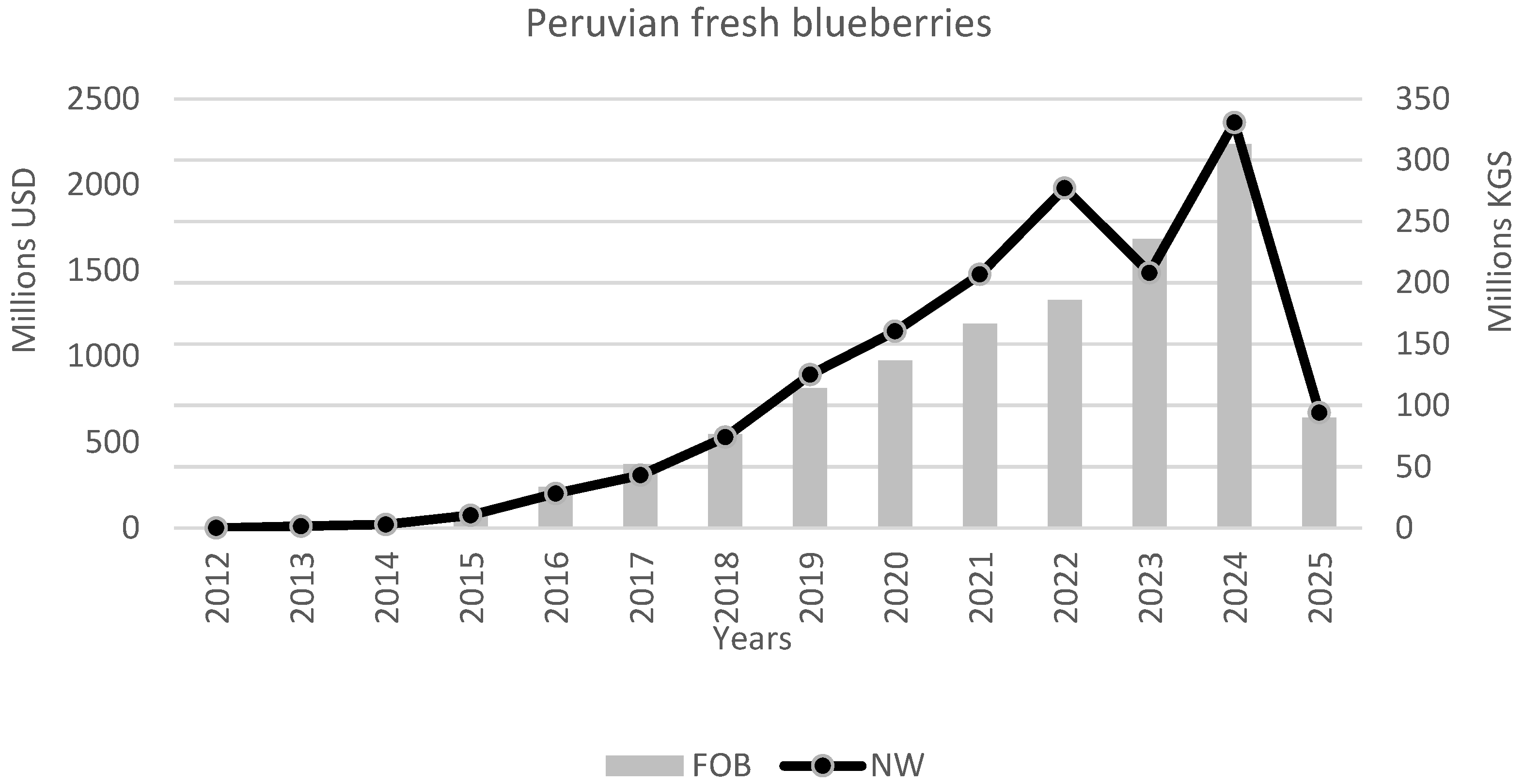
Peruvian fresh blueberry exports started in 2012 with very low FOB values and volumes, followed by a period of accelerated growth that extended until 2024. Export volumes exhibited a similar expansion pattern, whereas export unit prices showed a declining trend over most of the period under analysis.

3.1. Descriptive Analysis of Peruvian Fresh Blueberry Exports

Table 1. FOB value, export volume and unit price of Peruvian fresh blueberries (2012–2025).

Year	FOB Value	Export Volume (kg)	Unit Price (USD)
2012	465,204	47,916	9.71
2013	17,386,084	1,513,091	11.49
2014	29,968,033	2,902,124	10.33
2015	96,657,493	10,350,511	9.34
2016	241,285,935	28,154,433	8.57
2017	371,929,426	43,070,773	8.64
2018	546,287,357	74,021,076	7.38
2019	814,640,081	125,044,529	6.51
2020	974,514,809	160,361,099	6.08
2021	1,188,163,440	206,708,660	5.75
2022	1,326,654,134	277,018,073	4.79
2023	1,683,222,584	208,036,387	8.09
2024	2,235,165,160	330,529,889	6.76
2025	641,924,682	94,082,969	6.82

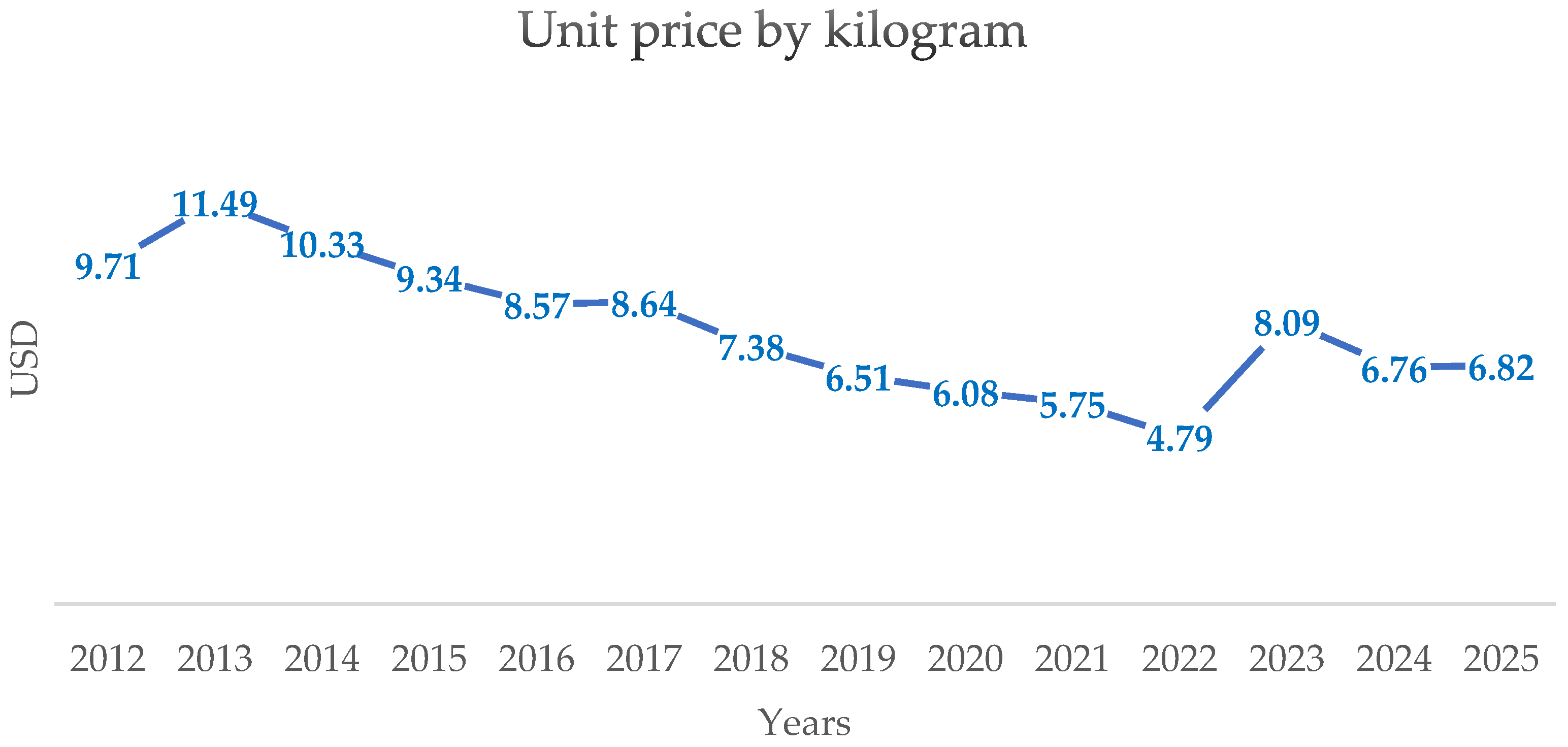
Note: Data for the years 2012–2014 were sourced from UN-Comtrade. Values for the period 2015–2025 were obtained from Veritrade.

summarizes the evolution of Peruvian fresh blueberry exports in terms of FOB value, export volume, and unit price between 2012 and 2025. The series shows a clear expansion in both FOB value and volume, from marginal levels in the early years to more than USD 2 billion and over 300 million kilograms in 2024, respectively. By contrast, the unit FOB price follows a more unstable trajectory, with a general downward trend until 2022, followed by a temporary recovery and subsequent adjustment. 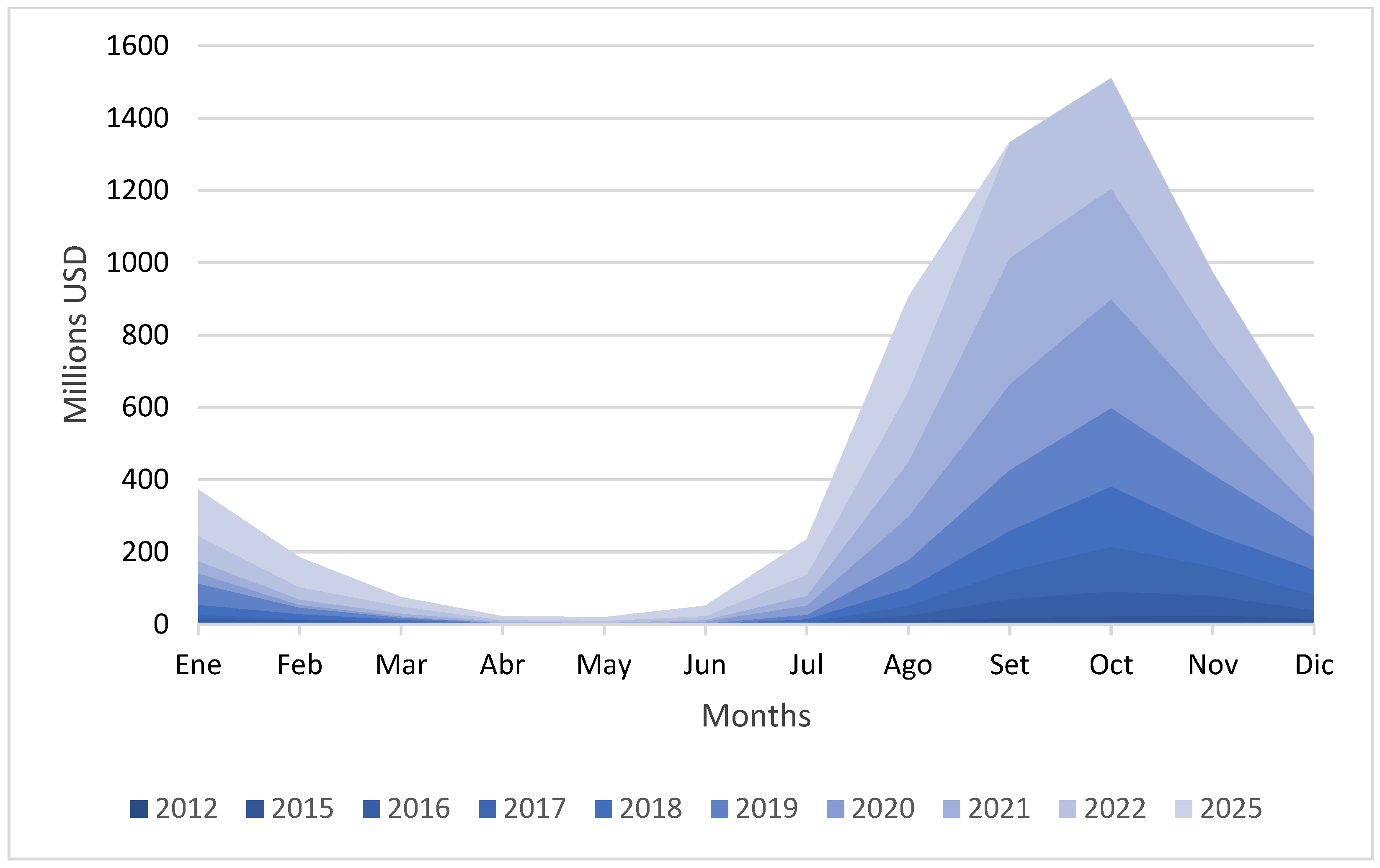In addition, Figure A1 (Appendix A) shows that export activity is markedly concentrated in the second half of the year, confirming the strong seasonal profile of the sector.

Figure 1 confirms that export value and volume moved broadly in the same direction throughout most of the period, reflecting the rapid scale-up of the sector. At the same time, the divergence between both series in selected years is consistent with the weaker and more volatile behavior of unit prices.

In addition,

Table 2. Peru’s Export Ranking and Number of Destination Markets for Fresh Blueberries (2012–2024).

Year	Rank PE	Countries
2024	4	44
2023	5	44
2022	9	33
2021	10	35
2020	8	35
2019	9	36
2018	14	29
2017	19	31
2016	21	27
2015	42	20
2014	101	18
2013	161	15
2012	***	7

Note: Data on Peru’s national export ranking (Rank PE) was obtained from SUNAT, while information on the number of destination markets was sourced from MINCETUR. *** indicates that, In 2012, the product ranked below the 499th position in the national export ranking.

complements this evidence by showing Peru’s growing position in global fresh blueberry exports and the widening number of destination markets. Between 2012 and 2024, export destinations increased from 7 to 44, while the product moved from a marginal rank in Peru’s export basket to a top-five position, confirming both the international consolidation and the strategic relevance of the sector.

3.2. Growth, Seasonality and Price Dynamics

To characterize the evolution of export value and volume, arithmetic mean, geometric mean, and compound annual growth rate (CAGR) weighting methods were examined. The results show that the arithmetic mean is highly sensitive to extreme observations, particularly in months with rapid shifts from very low to very high export levels, whereas the geometric mean provides a more stable summary but is less responsive to smaller month-to-month variations (see Supplementary Tables S6 and S7 for the higher average dispersion implied by both methods). For this reason, CAGR-based comparisons were used as a more informative descriptive benchmark.

The geometric mean exhibits greater stability in weighting; however, it is less sensitive to small variations, especially during the second half of the year from August to December.

A specific issue arises in 2012, when several months recorded zero exports. To avoid undefined percentage-growth calculations in the descriptive comparison of CAGR-based monthly variations, a temporary pseudo-count of 1 kg was assigned to those observations. This adjustment was used exclusively for descriptive growth comparisons and was not employed in the logarithmic estimations or in the forecasting models. Table S8 shows the descriptive CAGR comparison including the 2012 zero-export months, while

Table 3. Compound annual growth rate (CAGR) of FOB value and export volume (2013–2019).

Months	FOB Value %	Export Volume %
Jan	190.7	211.2
Feb	127.1	138.6
Mar	57.5	68.2
Apr	17.5	34.8
May	30.6	49.5
Jun	84.4	91.4
Jul	146.2	158.6
Aug	120.2	135.7
Set	96.2	119.4
Oct	86.8	110.6
Nov	83.4	101.5
Dec	75.7	90

Note: CAGR denotes the compound annual growth rate, calculated over the specified subperiods based on FOB values and export volumes.

reports the comparison starting in 2013.

Together, these results indicate that including the 2012 zero-export months produces much larger average variations, whereas the series becomes notably more regular when the comparison starts in 2013. This confirms that the post-2013 period provides a more stable basis for interpreting export growth dynamics. Such treatment is consistent with the broader literature noting that zero values require special handling in log-related transformations and growth comparisons [47,56].

Figure 2 reveals an inverse pattern relative to the joint evolution of FOB value and export volume. While both variables expanded over time, the unit price followed a broadly declining trajectory, reaching its highest level in 2013, falling until 2022, and then showing a partial recovery followed by a new adjustment. This divergence justifies treating value, volume, and price as related but distinct dimensions of export performance.

3.3. Definition of States and Classification in the Markov Model

This subsection presents the tables used to construct the base transition matrix for the Markov chain, starting from the minimum and maximum observed values of the export variables (Table S11). Four discrete states were defined for FOB value, export volume, and unit price (

Table 4. Percentiles and states defined under the Markov Chain framework.

Variable	State 1 (Low)	State 2 (Medium)	State 3 (High)	State 4 (Very High)
Ln (FOB value)	lnFOB ≤ p25	p25 < lnFOB ≤ p50	p50 < lnFOB ≤ p75	lnFOB > p75
Ln (Export volume)	lnKG ≤ p25	p25 < lnKG ≤ p50	p50 < lnKG ≤ p75	lnKG > p75
Ln (Unit price)	lnPRICE ≤ p25	p25 < lnPRICE ≤ p50	p50 < lnPRICE ≤ p75	lnPRICE > p75

Note: States were defined based on percentile thresholds of the logarithmic transformation of each variable.

). State thresholds were determined based on the 25th, 50th, and 75th percentiles of the empirical distribution (Table S12), given the presence of extreme values in the series.

In addition, in Table S13 (Supplementary Materials) natural logarithmic transformations were applied to the three variables in order to improve stability and suitability for Markov chain analysis.

Table 5. States and observed values for FOB value, export volume and unit price (2012).

t	FOB (USD)	Kg	Price	Ln-FOB	Ln-Kg	Ln-Price	Month	FOB-St	Kg-St	Price-St
0	2569	1100	2.34	7.85	7.00	0.85	January	St1	St1	St1
1	122	913	0.13	4.80	6.82	−2.01	February	St1	St1	St1
2	34	258	0.13	3.54	5.55	−2.02	March	St1	St1	St1
3	23,358	1953	11.96	10.06	7.58	2.48	August	St1	St1	St4
4	149,337	12,524	11.92	11.91	9.44	2.48	September	St1	St1	St4
5	125,229	11,535	10.86	11.74	9.35	2.38	October	St1	St1	St4
6	81,499	9758	8.35	11.31	9.19	2.12	November	St1	St1	St3
7	83,056	9876	8.41	11.33	9.20	2.13	December	St1	St1	St3

Note: States were defined based on percentile thresholds of the logarithmic transformation of each variable.

reports the classification results for the year 2012. In total, 160 valid observations were considered. Because export value and volume exhibited extreme values, logarithmic specifications were employed for subsequent projections and modeling tests.

3.4. Seasonal Markov Transition Matrices for FOB, Export Volume, and Unit Price

Table 6. State of season transition probability matrix (2012–2025).

Stations	Summer	Autumn	Winter	Spring	Total
Summer	65.85%	34.15%	0.00%	0.00%	100.0%
Autumn	0.00%	65.00%	35.00%	0.00%	100.0%
Winter	0.00%	0.00%	66.67%	33.33%	100.0%
Spring	33.33%	0.00%	0.00%	66.67%	100.0%

Note: Transition probabilities were estimated from observed state transitions over the period 2012–2025. Rows represent the current state, while columns represent the subsequent state.

shows that seasonal transitions are dominated by persistence, as the probability of remaining in the same season exceeds 65% in all cases. When transitions do occur, they are concentrated in the adjacent seasonal shifts that reflect the underlying agricultural calendar, especially from summer to autumn, autumn to winter, winter to spring, and spring to summer. This pattern supports the view that blueberry export dynamics evolve within a stable but cyclical seasonal framework.

Table 7. Autumn state transition probabilities for FOB value, export volume and price.

From\To	Low (St1)	Medium (St2)	High (St3)	Very High (St4)	Total
Matrix probability Ln-FOB (Autumn)
St1	89.5%	10.5%	0.0%	0.0%	100.0%
St2	33.3%	60.0%	6.7%	0.0%	100.0%
St3	0.0%	0.0%	100.0%	0.0%	100.0%
St4	55.0%	35.0%	7.5%	2.5%	100.0%
Matrix probability Ln-Kg (Autumn)
St1	88.9%	11.1%	0.0%	0.0%	100.0%
St2	38.9%	50.0%	11.1%	0.0%	100.0%
St3	0.0%	75.0%	25.0%	0.0%	100.0%
St4	0.0%	0.0%	0.0%	0.0%	100.0%
Matrix probability Ln-Price (Autumn)
St1	40.0%	50.0%	0.0%	10.0%	100.0%
St2	9.1%	45.5%	36.4%	9.1%	100.0%
St3	0.0%	22.2%	33.3%	44.4%	100.0%
St4	0.0%	10.0%	40.0%	50.0%	100.0%

Note: The table reports transition probabilities estimated from observed autumn state transitions during 2012–2025. Rows correspond to the current state, whereas columns correspond to the subsequent state.

indicates that the autumn transition structure is not uniform across the three export dimensions. FOB value and export volume remain comparatively stable, especially in the lower states, suggesting stronger persistence during this season. Unit price, however, displays a more mobile transition pattern, with relevant movements between upper adjacent states, particularly from the high to the very high state (44.4%) and from the very high to the high state (40.0%). This suggests a more volatile price dynamic relative to value and volume.

This pattern also varies across seasons. Spring appears to be the most stable season overall, as FOB value and export volume remain in the same state with persistence probabilities ranging from 85.7% to 100% and from 91.7% to 100%, respectively (

Table A1. Seasonal transition probability matrix for FOB value by season.

From\To	Low (St1)	Medium (St2)	High (St3)	Very High (St4)
Summer (Dec–Feb)
St1	83.30%	16.70%	0.00%	0.00%
St2	33.30%	66.70%	0.00%	0.00%
St3	0.00%	43.80%	56.30%	0.00%
St4	0.00%	0.00%	40.00%	60.00%
Autumn (Mar–May)
St1	89.50%	10.50%	0.00%	0.00%
St2	33.30%	60.00%	6.70%	0.00%
St3	0.00%	0.00%	100.00%	0.00%
St4	55.00%	35.00%	7.50%	2.50%
Winter (Jun–Aug)
St1	50.00%	50.00%	0.00%	0.00%
St2	0.00%	18.20%	81.80%	0.00%
St3	0.00%	0.00%	33.30%	66.70%
St4	0.00%	0.00%	0.00%	100.00%
Spring (Sep–Nov)
St1	100.00%	0.00%	0.00%	0.00%
St2	0.00%	80.00%	20.00%	0.00%
St3	0.00%	0.00%	80.00%	20.00%
St4	0.00%	0.00%	14.30%	85.70%

Note: Seasonal transition matrices were constructed by conditioning state transitions on meteorological seasons, as defined by SENAMHI.

and

Table A2. Seasonal transition probability matrix for export volume by season.

From\To	Low (St1)	Medium (St2)	High (St3)	Very High (St4)
Summer (Dec–Feb)
St1	83.30%	16.70%	0.00%	0.00%
St2	0.00%	100.00%	0.00%	0.00%
St3	0.00%	41.20%	58.80%	0.00%
St4	0.00%	0.00%	60.00%	40.00%
Autumn (Mar–May)
St1	88.90%	11.10%	0.00%	0.00%
St2	38.90%	50.00%	11.10%	0.00%
St3	0.00%	75.00%	25.00%	0.00%
St4	0.00%	0.00%	0.00%	0.00%
Winter (Jun–Aug)
St1	50.00%	50.00%	0.00%	0.00%
St2	0.00%	18.20%	81.80%	0.00%
St3	0.00%	0.00%	33.30%	66.70%
St4	0.00%	0.00%	0.00%	100.00%
Spring (Sep–Nov)
St1	100.00%	0.00%	0.00%	0.00%
St2	0.00%	100.00%	0.00%	0.00%
St3	0.00%	0.00%	100.00%	0.00%
St4	0.00%	0.00%	8.30%	91.70%

Note: Seasonal transition matrices were constructed by conditioning state transitions on meteorological seasons, as defined by SENAMHI.

). Unit price follows the same general pattern, although at lower levels, with same-state persistence ranging from 63.2% to 85.7% (

Table A3. Seasonal transition probability matrix for unit price by season.

From\To	Low (St1)	Medium (St2)	High (St3)	Very High (St4)
Summer (Dec–Feb)
St1	76.20%	19.00%	4.80%	0.00%
St2	22.20%	55.60%	11.10%	11.10%
St3	30.00%	10.00%	40.00%	20.00%
St4	0.00%	100.00%	0.00%	0.00%
Autumn (Mar–May)
St1	40.00%	50.00%	0.00%	10.00%
St2	9.10%	45.50%	36.40%	9.10%
St3	0.00%	22.20%	33.30%	44.40%
St4	0.00%	10.00%	40.00%	50.00%
Winter (Jun–Aug)
St1	50.00%	0.00%	0.00%	50.00%
St2	6.70%	60.00%	26.70%	6.70%
St3	0.00%	0.00%	58.30%	41.70%
St4	10.00%	20.00%	0.00%	70.00%
Spring (Sep–Nov)
St1	85.70%	0.00%	14.30%	0.00%
St2	60.00%	40.00%	0.00%	0.00%
St3	12.50%	37.50%	50.00%	0.00%
St4	0.00%	0.00%	36.80%	63.20%

Note: Seasonal transition matrices were constructed by conditioning state transitions on meteorological seasons, as defined by SENAMHI.

). Winter, by contrast, is especially notable in the very high state (St4): FOB value and export volume remain fully persistent at 100%, whereas unit price shows a somewhat lower but still substantial persistence of 70.0% (Table A1, Table A2 and Table A3).

Table 8. Main seasonal state transitions across FOB value, export volume, and unit price.

Value (FOB Value)	Export Volume	Unit Price	Season
Medium to low 33%	Very high to high 60%	Very high to medium 100%	Summer
Very high to low 55%	High to medium 75%	Low to medium 50%	Autumn
Medium to high 82%	Medium to high 82%	High to very high 42%	Winter
Very high to high 14%	Very high to high 8%	Medium to low 60%	Spring

Note: Transition probabilities were estimated from observed state transitions over the period 2012–2025.

provides a synthetic view of the main state changes across seasons and confirms that the three export dimensions do not evolve under a common transition logic. FOB value and export volume are mainly driven by corrections between adjacent or upper states, whereas unit price displays more diverse movements across the state distribution. This heterogeneity suggests that seasonal state dynamics differ substantially between value, volume, and price, supporting the need for a comparative forecasting framework rather than a single uniform modeling strategy.

3.5. Forecast Comparison: Markov–Monte Carlo, Log-Linear Growth and SARIMA

To assess the relative forecasting performance of the three modeling approaches, out-of-sample forecasts were generated and evaluated using standard accuracy metrics.

Table 9. Comparative forecast accuracy of Markov–Monte Carlo, log-linear growth, and SARIMA models.

Variable	Scale	Model	Rank	MAE	RMSE
FOB value	Level	LLG	1	54.82	80.8
	Level	MMC	2	62.59	91.01
	Level	SARIMA	3	99.12	159.44
	Logarithmic	LLG	1	1.0018	1.1431
	Logarithmic	SARIMA	2	1.1843	1.4143
	Logarithmic	MMC	3	3.378	3.5813
Export volume	Level	SARIMA	1	73.28	93.97
	Level	MMC	2	118.94	168.58
	Level	LLG	3	350.18	378.11
	Logarithmic	SARIMA	1	1.3072	1.544
	Logarithmic	MMC	2	1.7973	2.0954
	Logarithmic	LLG	3	2.987	3.6157
Unit price	Level	MMC	1	0.49	0.74
	Level	SARIMA	2	0.94	1.11
	Level	LLG	3	7.66	7.74
	Logarithmic	MMC	1	0.0686	0.1099
	Logarithmic	SARIMA	2	0.1254	0.1466
	Logarithmic	LLG	3	0.208	0.2343

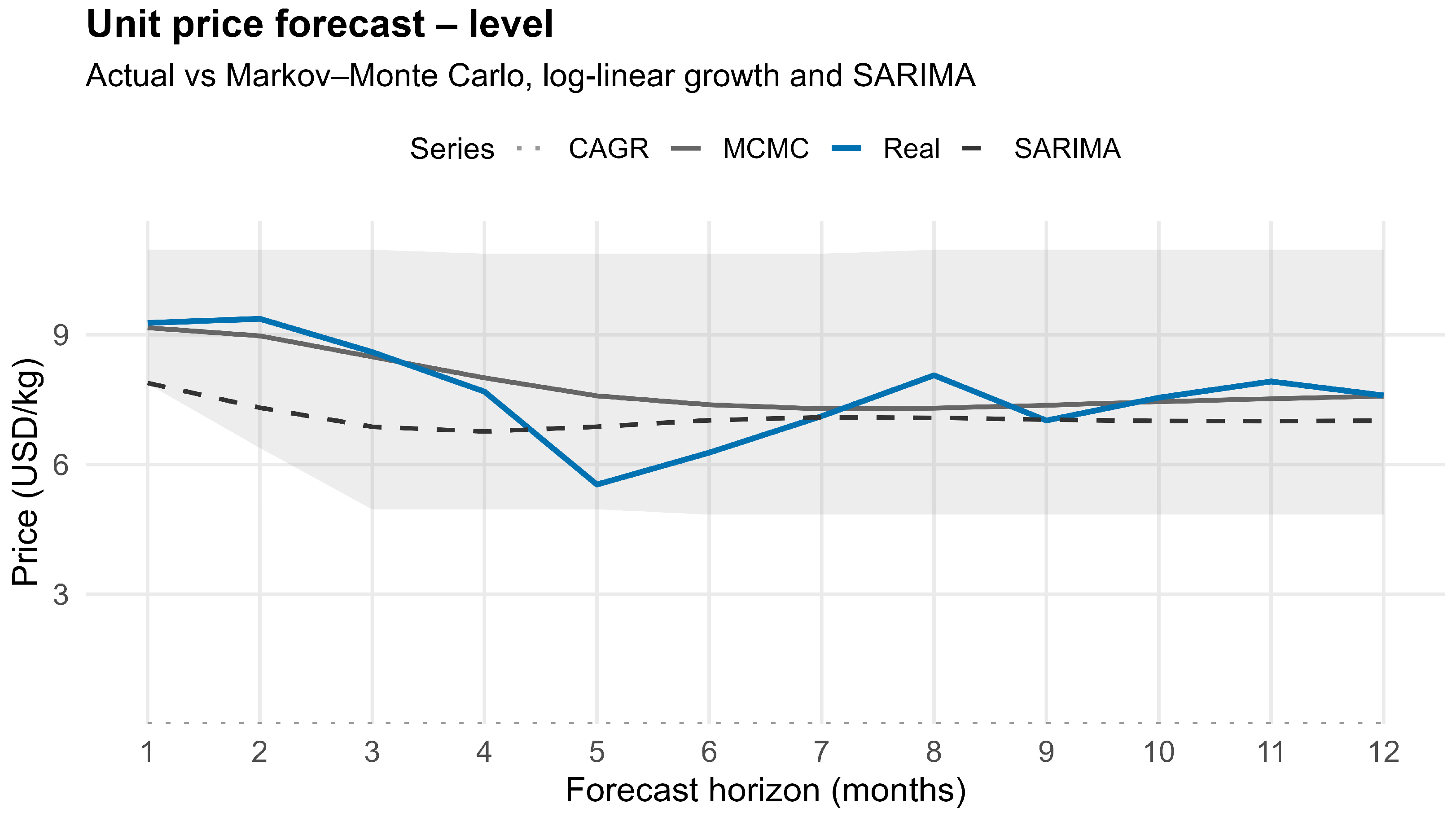
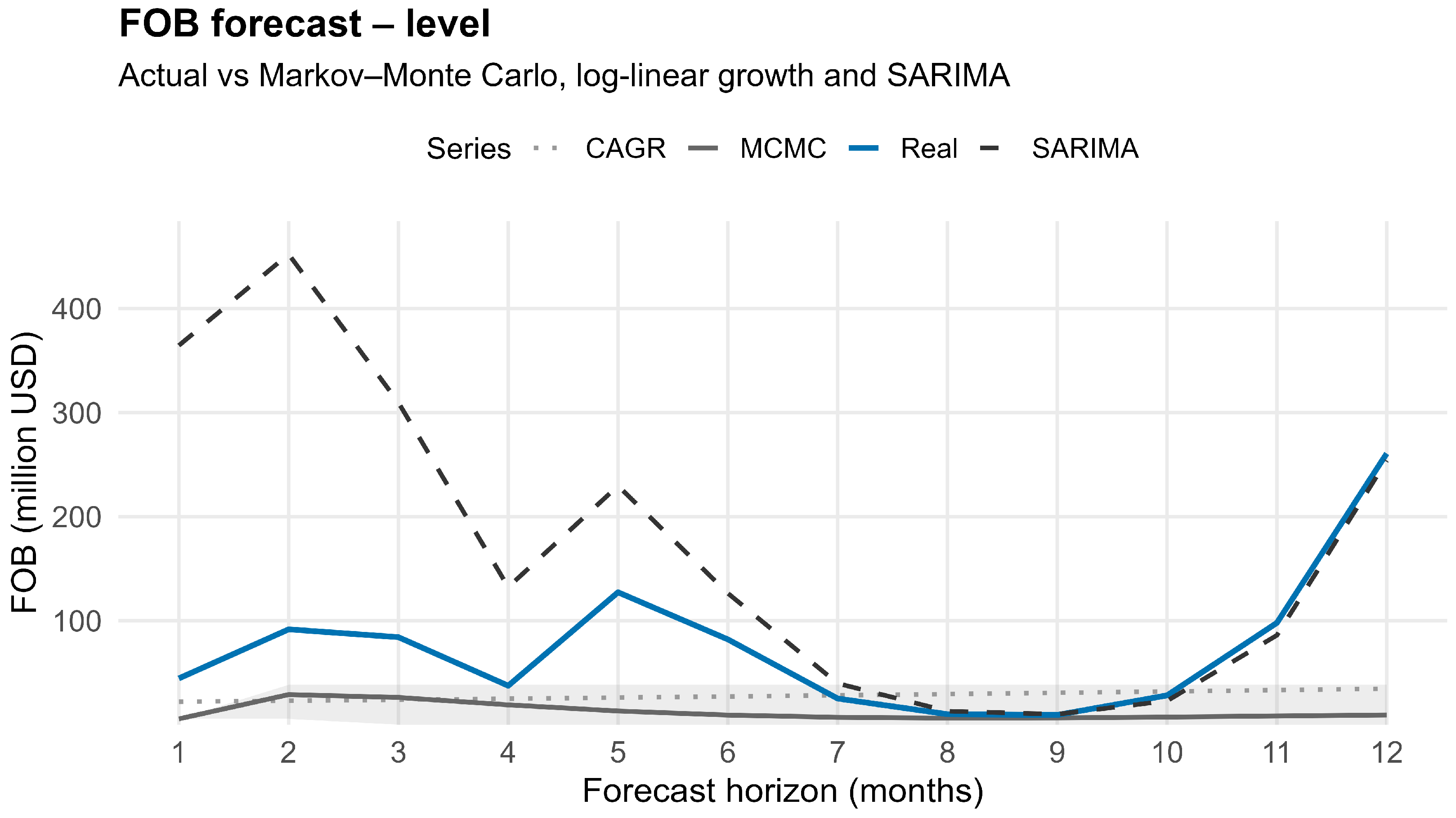
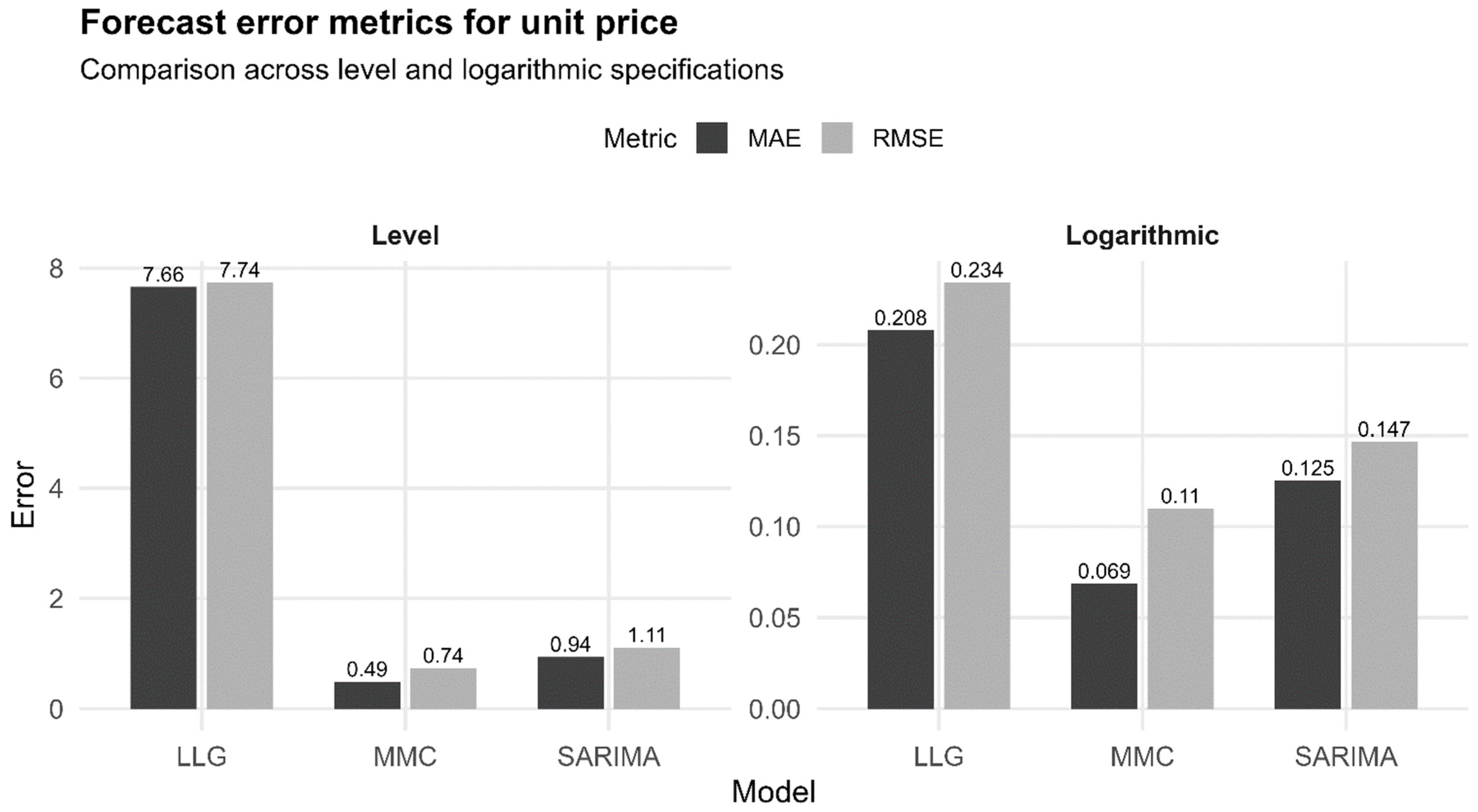
Note: The table reports out-of-sample forecast errors for the 12-month test period. Rank is based on RMSE within each variable–scale combination. Bold values indicate the lowest error within each variable–scale combination. LLG denotes the log-linear growth model, MMC the Markov–Monte Carlo model, and SARIMA the seasonal autoregressive integrated moving average model.

provides a consolidated comparison of forecast accuracy across FOB value, export volume, and unit price, in both level and logarithmic specifications, allowing a direct assessment of how model performance varies across scales. The results show that no single model dominates across all dimensions: log-linear growth performs best for FOB, SARIMA for export volume, and Markov–Monte Carlo for unit price. 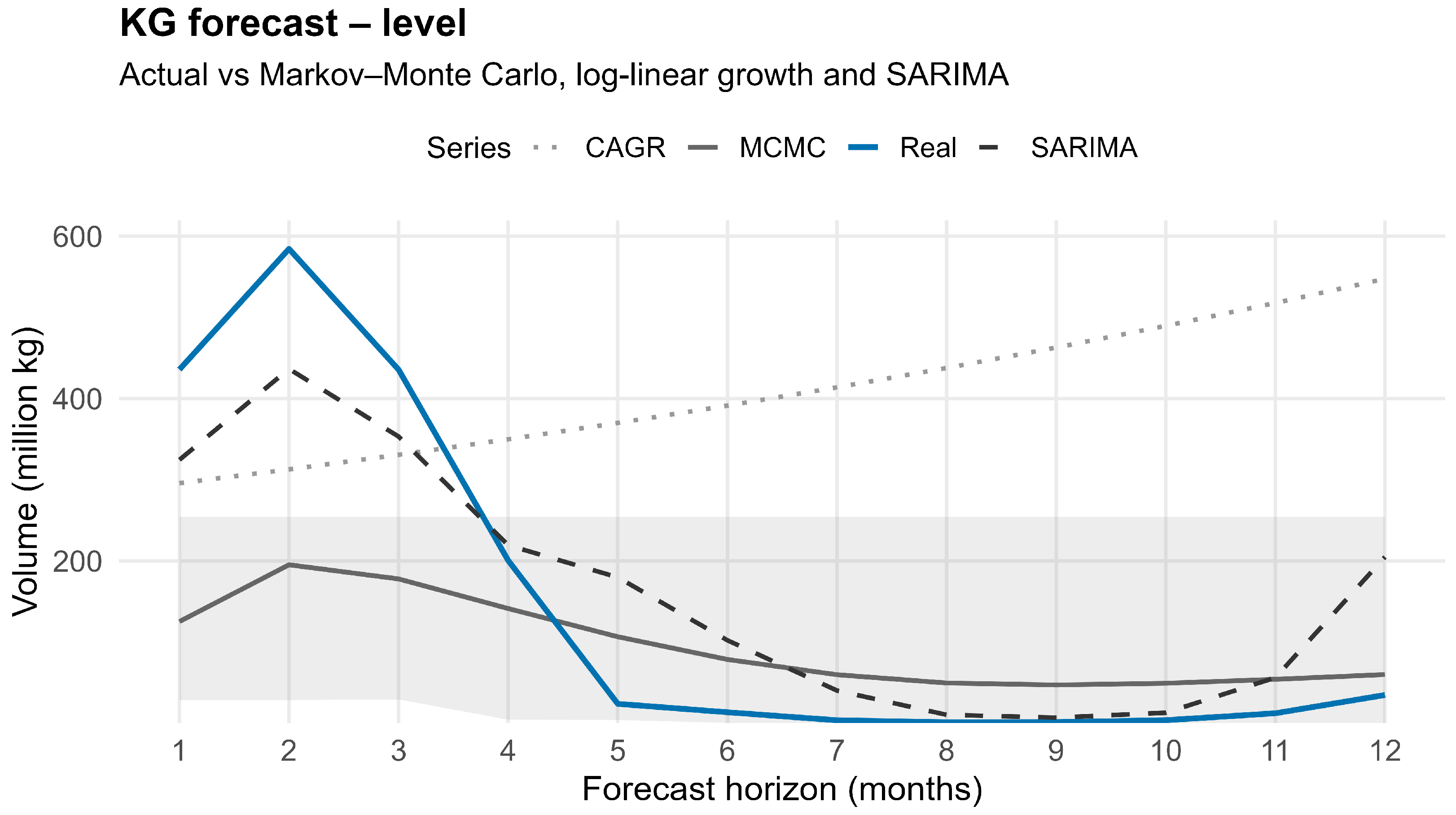Figure 3, Figure 4 and Figure 5 complement this comparison by illustrating the corresponding forecast trajectories in level terms. 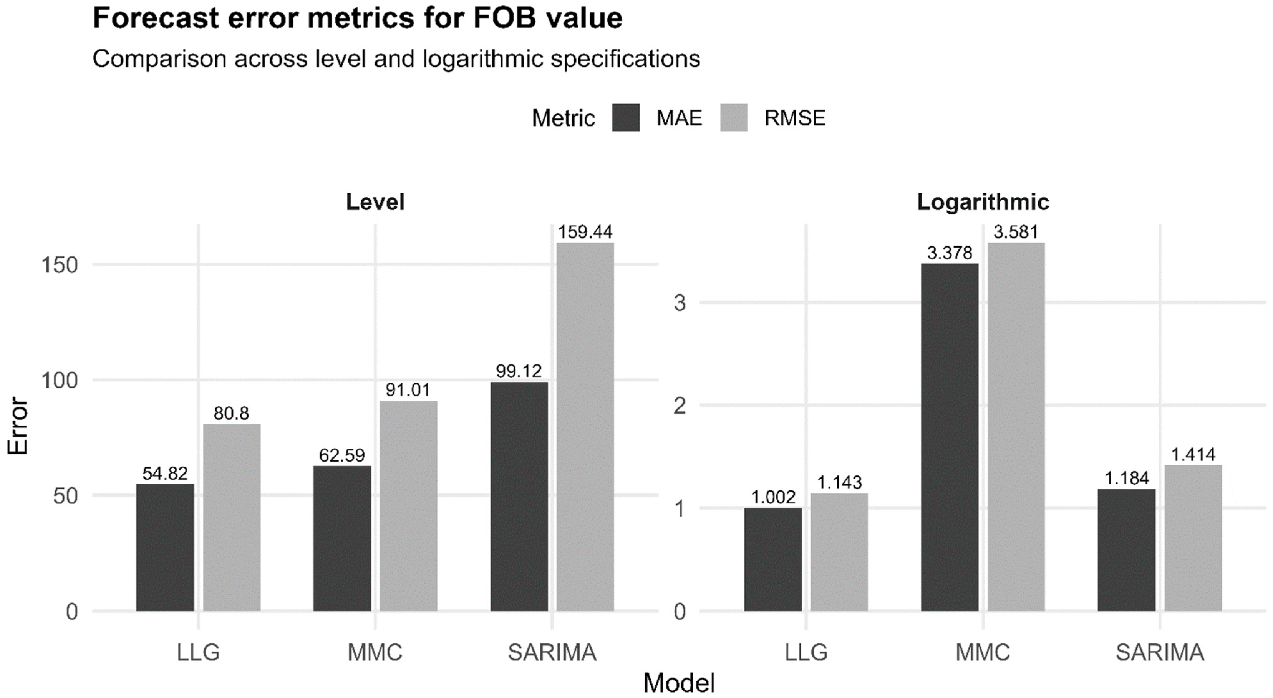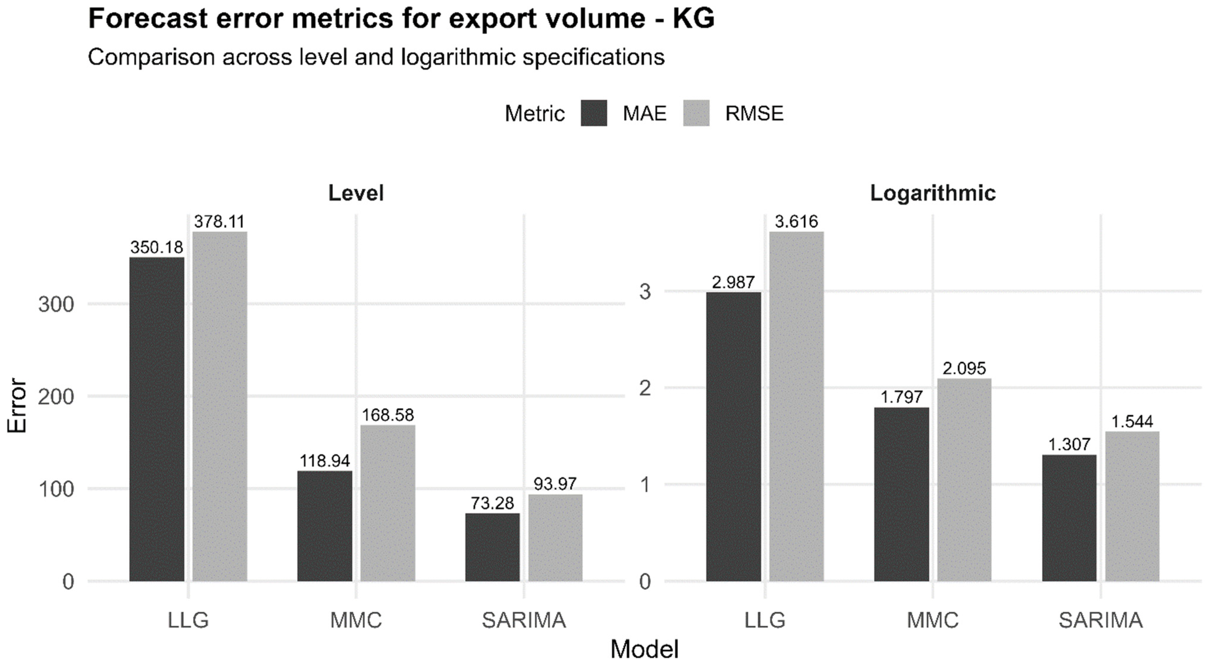The analogous visual comparisons in logarithmic scale are reported in Figures S1–S3, while the associated error-metric summaries are presented in Figure A2, Figure A3 and Figure A4.

In the main-text forecast figures, uncertainty is represented using the simulated 5th–95th percentile band of the Markov–Monte Carlo forecasts. This choice provides an explicit visual summary of forecast uncertainty while maintaining a clear and comparable presentation of the three competing approaches. Complementary logarithmic-scale comparisons are reported in the Supplementary Material, whereas the corresponding error-metric summaries are presented in Appendix C.

3.5.1. Forecast Performance for Export Values (FOB)

The comparative evaluation of the three forecasting approaches reveals clear differences in predictive accuracy for FOB values. As shown in Table 9, the log-linear growth model achieves the lowest MAE and RMSE in both level and logarithmic specifications, indicating that the strong trend component of export values dominates short-term fluctuations over the evaluation horizon. Figure 3 confirms this result visually, as the log-linear growth trajectory follows the observed path more closely than the alternative models.

3.5.2. Forecast Performance for Export Volumes

For export volume, the results differ from those obtained for FOB values. Table 9 shows that SARIMA provides the lowest MAE and RMSE in both level and logarithmic specifications, suggesting that volume dynamics are more strongly influenced by recurring seasonal patterns and short-term dependence than by a smooth deterministic trend. Figure 4 supports this interpretation, as the SARIMA trajectory more closely tracks the observed series over the test horizon than the competing approaches.

3.5.3. Forecast Performance for Export Prices

Unit price displays a distinct forecasting pattern relative to FOB values and export volume. According to Table 9, the Markov–Monte Carlo approach yields the lowest MAE and RMSE in both level and logarithmic specifications, outperforming both SARIMA and the log-linear growth model. This result suggests that price dynamics are more sensitive to state-dependent changes and nonlinear adjustments than to deterministic trend extrapolation. Figure 5 visually reinforces this finding, showing that the Markov–Monte Carlo forecasts remain closer to the observed trajectory than the alternative models. The uncertainty band shown in Figure 5 further illustrates the distributional range associated with the Markov–Monte Carlo forecasts.

3.6. Robustness and Sensitivity Checks

This subsection evaluates the robustness of the forecasting results through residual diagnostics and sensitivity checks. In particular, residual behavior is examined to assess whether model assumptions are satisfied and whether forecast accuracy is supported by adequate statistical properties.

3.6.1. Residual Diagnostics on the Full Sample (2012–2025)

The residual behavior of the SARIMA models estimated over the full sample period (2012–2025) was first examined. Figures S4–S6 display the residual diagnostics for the ln(FOB), ln(export volume), and ln(unit price) series, respectively, including the time path of residuals, the autocorrelation function, and the histogram with normal density overlay. Visual inspection shows that residuals fluctuate around zero without systematic patterns or pronounced residual seasonality.

Table 10. Ljung–Box test results for SARIMA residuals in the full sample.

Variable	Q-Statistic	df	p-Value
FOB Value	21.50254	24	0.608932
Export Volume	15.69989	24	0.898603
Unit Price	10.92558	24	0.989533

Note: Ljung–Box test statistics were computed to assess residual autocorrelation at 24 lags. The null hypothesis is that residuals are not serially correlated.

summarizes the Ljung–Box test results for the SARIMA residuals computed at 24 lags over the full sample period. For all three variables, the associated p-values remain above the conventional 5% significance threshold, indicating no evidence against the null hypothesis of white noise.

3.6.2. Residual Diagnostics on the Training Period

The residual analysis was then replicated using only the training period employed for forecast evaluation. Figures S7–S9 present the residual diagnostics for the SARIMA models estimated over this subsample, while

Table 11. Ljung–Box test results for SARIMA residuals in the training period.

Variable	Q-Statistic	df	p-Value
FOB Value	20.86797	24	0.6465011
Export Volume	15.45075	24	0.9068744
Unit Price	10.48890	24	0.9922162

Note: Ljung–Box test statistics were computed to assess residual autocorrelation at 24 lags for the training subsample. The null hypothesis is that residuals are not serially correlated.

reports the corresponding Ljung–Box test results. Consistent with the previous analysis, residuals remain centered around zero and show no evidence of significant autocorrelation at 24 lags with p-values above the conventional 5% significance threshold.

3.6.3. Comparison of Residual Patterns Across FOB, Volume and Price

The comparison of residual patterns across the three variables reveals notable differences in their underlying dynamics. For ln(export volume), residuals are more tightly concentrated around zero and the histogram closely approximates a normal distribution, resulting in relatively low Q* statistics and high p-values.

For ln(FOB value), a higher degree of dispersion is observed, together with isolated peaks in the autocorrelation function. These features are consistent with episodes of volatility associated with international price shocks and fluctuations in exported volumes.

In the case of ln(unit price), residuals display moderate asymmetry, suggesting that although the seasonal and trend components are adequately captured, idiosyncratic price shocks remain that are not fully explained by the univariate specification. Nevertheless, across all three variables, the overall diagnostics are consistent with approximately uncorrelated residuals and stable variance.

3.6.4. Implications for Forecast Risk and Robustness

Residual diagnostics complement the evidence on forecast accuracy reported in previous subsections. In level specifications, the log-linear growth model achieves lower point forecast errors for ln(FOB value) and ln(export volume), whereas the Markov–Monte Carlo approach tends to produce higher error values. By contrast, SARIMA models exhibit favorable statistical properties of the residuals, including the absence of significant autocorrelation and stable variance, supporting their use for the construction of forecast intervals and risk assessment.

From a forecast risk perspective, the combination of moderate error levels (MAE and RMSE) with residuals behaving as white noise indicates that forecast uncertainty is primarily driven by unpredictable shocks rather than by systematic model bias. This feature is particularly relevant for ln(FOB value), where residual volatility is consistent with periods of heightened instability in international markets. For ln(export volume), the lower dispersion of residuals suggests more regular underlying dynamics, resulting in comparatively stable projections under the SARIMA framework.

For ln(unit price), the presence of mild residual asymmetry points to the potential relevance of extensions that allow for regime changes or heteroskedasticity, such as SARIMA–GARCH models, in future research. Nevertheless, the current results remain statistically acceptable for scenario analysis purposes.

Overall, residual diagnostics confirm that the SARIMA models employed in this study are statistically consistent over both the training sample and the full sample period. While the log-linear growth model often provides better point accuracy in terms of MAE and RMSE, SARIMA models offer a solid basis for uncertainty quantification and risk analysis, which supports their joint use with the Markov–Monte Carlo approach and compound growth measures in the evaluation of export strategies.

4. Discussion

The findings of this study reveal substantial differences in the performance and suitability of alternative forecasting approaches for Peruvian fresh blueberry exports, depending on the variable under analysis and the evaluation criterion applied. When deterministic benchmarks such as log-linear growth models are employed, the resulting trajectories tend to be smooth and trend-dominated, closely reflecting the strong expansion path observed in FOB export values during most of the sample period. This result suggests that, in contexts characterized by sustained growth, parsimonious trend-based models remain effective for short-term point forecasting, particularly for aggregate export values.

At the same time, the empirical evidence confirms that blueberry exports exhibit pronounced seasonality and regime-dependent behavior, consistent with the biological cycle of production and the organization of international logistics. The seasonal Markov transition matrices show a high degree of persistence within states and systematic transitions aligned with the agricultural calendar. Winter months display a higher probability of upward transitions in export value and volume, whereas summer and spring are more frequently associated with lower states. These results are in line with previous agricultural trade studies [38,39] that emphasize the usefulness of Markov chains for identifying persistence and transition dynamics across export performance levels.

From a forecasting accuracy perspective, the comparison across models highlights that no single approach dominates across all variables. For FOB export values, the log-linear growth model yields the lowest MAE and RMSE in level specifications, indicating that the dominant trend component outweighs short-term fluctuations over the evaluation horizon. This finding is consistent with classical econometric evidence [36,37] suggesting that, in rapidly expanding export sectors, deterministic growth models can provide reliable short-run approximations.

In contrast, for export volumes and especially for unit prices, stochastic models perform more favorably. SARIMA models exhibit superior accuracy for export volumes and display strong residual properties, including the absence of significant autocorrelation and stable variance. These results support earlier contributions that highlight the suitability of seasonal ARIMA specifications for monthly agricultural and trade-related series, particularly when seasonality and short-term dependence are relevant [57].

Price dynamics show a distinct pattern. Export unit prices are more volatile and exposed to international market shocks, which reduces the explanatory power of simple trend-based models. In this context, the Markov–Monte Carlo approach outperforms both SARIMA and log-linear growth models in terms of forecast accuracy. This result is consistent with the literature on commodity prices and regime-switching behavior [21,33], which documents that price series often follow nonlinear dynamics characterized by persistence within regimes and abrupt transitions driven by external shocks.

The Markov–Monte Carlo framework, while not always minimizing point forecast errors, provides additional insights that are not captured by purely deterministic or linear stochastic models. By explicitly modeling discrete states and seasonal regimes, it allows the identification of persistence patterns, transition probabilities, and risk bands derived from simulated distributions. This feature is particularly valuable for scenario analysis and risk management, even when conventional error metrics penalize the dispersion of simulated paths.

Residual diagnostics further reinforce these conclusions. SARIMA models display residuals that behave approximately as white noise across both the training and full samples, supporting their statistical adequacy and their use for uncertainty quantification. The higher dispersion observed in FOB residuals is consistent with episodes of international market instability, whereas export volumes exhibit more regular dynamics. For prices, mild residual asymmetry suggests that future extensions incorporating regime-switching volatility or heteroskedastic structures could further improve model performance.

Overall, the evidence supports a complementary interpretation of forecasting tools. Deterministic growth models are effective for capturing dominant trends in aggregate export values, SARIMA models offer a robust framework for seasonal adjustment and risk assessment, and Markov–Monte Carlo approaches enrich the analysis by capturing regime dependence and nonlinear dynamics. Their combined use therefore provides a more comprehensive representation of agricultural export behavior than any single method. To make this interpretation more directly applicable,

Table 12. Simplified decision framework for forecasting model selection.

Model	Best Suited for	Key Strength	Best Result
LLG	Stable growth paths	Simplicity	FOB value
SARIMA	Seasonal dependence	Statistical fit	Export volume
MMC	Regime shifts	Risk insight	Unit price

Note: LLG = log-linear growth; MMC = Markov–Monte Carlo. “Best suited for” summarizes the dominant data condition under which each model is more informative. “Best result” identifies the export dimension for which the model performed most favorably in the present study.

presents a simplified decision framework indicating the conditions under which each model is most informative, its main practical strength, and the export dimension for which it performed most favorably in the present study.

Beyond differences in statistical performance, the three forecasting approaches also involve distinct computational and practical trade-offs. Log-linear growth models are the most parsimonious and easiest to implement, requiring minimal specification decisions and offering highly interpretable short-term extrapolations. Seasonal SARIMA models involve greater modeling effort, including order selection, residual checking, and sensitivity to specification, but they provide a stronger framework for representing monthly dependence, seasonality, and statistically coherent forecast intervals.

Markov–Monte Carlo models require the highest degree of design and computational effort, since their performance depends on state construction, transition-matrix estimation, and the stability of simulated trajectories. However, this additional complexity is compensated by their ability to capture regime persistence, nonlinear adjustment, and uncertainty ranges that are especially valuable for scenario analysis and export-risk assessment.

From a theoretical standpoint, the findings support a plural modeling view of export forecasting, in which predictive adequacy depends on the temporal structure of the variable under analysis rather than on the unconditional superiority of any single methodological class.

5. Conclusions

This study examined the export dynamics of Peruvian fresh blueberries by jointly applying and comparing three forecasting approaches—Markov–Monte Carlo, log-linear growth, and SARIMA—to export value (FOB), export volume, and unit price over the period 2012–2025. By integrating descriptive analysis, seasonal Markov transition matrices, forecast accuracy metrics, and residual diagnostics, the research provides a comprehensive evaluation of model performance across multiple dimensions of the export value chain.

The results demonstrate that no single forecasting model uniformly outperforms the others. Log-linear growth models yield accurate and parsimonious short-term forecasts for export values, reflecting the strong trend component associated with Peru’s rapid expansion as a global blueberry exporter. SARIMA models show superior performance for export volumes and exhibit favorable statistical properties, making them particularly suitable for uncertainty quantification and risk analysis. Markov–Monte Carlo models, while less competitive in terms of point forecast errors, provide valuable insights into seasonal regimes, persistence, and state-dependent dynamics, especially for unit prices.

Seasonality emerges as a central determinant of export behavior. The seasonal Markov transition matrices reveal high persistence within states and systematic transitions aligned with the agricultural calendar, underscoring the importance of explicitly accounting for seasonal regimes when modeling Agricultural export series. Differences across export value, volume, and price highlight the heterogeneous nature of the export chain, with prices displaying greater volatility and benefiting more from nonlinear and regime-based modeling approaches.

Residual diagnostics confirm the statistical consistency of the SARIMA models and indicate that remaining forecast uncertainty is largely driven by exogenous shocks rather than systematic misspecification. This reinforces the importance of combining forecast accuracy measures with diagnostic analysis when evaluating competing models.

From an applied perspective, the findings suggest that exporters and policymakers should not rely on a single forecasting tool. Instead, a combined framework that integrates deterministic growth benchmarks, seasonal SARIMA models, and Markov–Monte Carlo simulations offers a more flexible and informative basis for decision-making. Such an approach supports production planning, logistics coordination, market access strategies, and risk management in dynamic agricultural export sectors.

From a practical standpoint, the results suggest a simple decision framework for model selection. Log-linear growth models are most appropriate when export series are dominated by a stable expansion trend and the main objective is parsimonious short-term point forecasting, as in FOB export values. Seasonal SARIMA models are preferable when monthly seasonality and short-run dependence are central to the data-generating process, as in export volumes. Markov–Monte Carlo models are especially useful when the analyst is interested not only in point forecasts but also in regime dependence, transition patterns, and uncertainty bands, particularly in more volatile dimensions such as unit prices.

While this study does not implement a formal forecast combination procedure, the results are consistent with the broader forecasting literature, suggesting that different models capture distinct dimensions of export dynamics. In this sense, subsequent studies could evaluate whether weighted or hybrid combinations of log-linear growth, SARIMA, and regime-based forecasts improve predictive stability across FOB value, export volume, and unit price [41,42,58].

Future research could extend this framework by incorporating multivariate specifications, regime-switching volatility models, or exogenous drivers such as climate indicators, logistics constraints, and international price indices. These extensions would further enhance the ability of forecasting models to capture structural changes and extreme events in global agricultural markets.

Although the empirical results are specific to Peruvian fresh blueberries, the comparative forecasting framework proposed in this study may be transferable to other agri-export commodities and exporting countries that share similar characteristics, such as marked seasonality, rapid export growth, structural breaks, or regime-sensitive price behavior. Products exposed to concentrated harvest windows, volatile international prices, and changing market-access conditions may benefit from a similar comparison between deterministic, autoregressive, and regime-based approaches. At the same time, the external validity of the substantive findings should be interpreted with caution, since model performance is likely to depend on the maturity of the export sector, the stability of seasonal patterns, and the availability of sufficiently consistent time-series data.

Limitations: An additional methodological limitation is that forecasts estimated in logarithmic scale were back-transformed using the simple exponential function, without an explicit bias correction. Although this may slightly underestimate level forecasts when residual variance is high, the effect is unlikely to modify the comparative interpretation of model performance because the same transformation rule was applied consistently across competing models. Another limitation is that the analysis compares individual forecasting models but does not estimate formal forecast combination schemes, which could be explored in future research to integrate deterministic, autoregressive, and regime-based predictive information [41,43].

References

- OECD/FAO. OECD-FAO Agricultural Outlook 2023–2032; OECD-FAO Agricultural Outlook; OECD: Paris, France, 2023; ISBN 9789264619333. [Google Scholar]
- Straume, H.M.; Asche, F.; Oglend, A.; Abrahamsen, E.B.; Birkenbach, A.M.; Langguth, J.; Lanquepin, G.; Roll, K.H. Impacts of COVID-19 on Norwegian Salmon Exports: A Firm-Level Analysis. Aquaculture 2022, 561, 738678. [Google Scholar] [CrossRef] [Scilit] [PubMed]
- Levard, L.; Mainenti, C.; Capdepon, E.; Compain, G. Las Lecciones de La Reciente Fuerte Subida de Los Precios Mundiales; C2A/Coordination SUD: Paris, France, 2021. [Google Scholar]
- USDA-Foreign Agricultural Service Blueberries Around the Globe—Past, Present, and Future; 2021. Available online: https://www.fas.usda.gov/data/blueberries-around-globe-past-present-and-future/ (accessed on 23 April 2026).
- Newman, M. Plant Talk: Neotropical Blueberries. Available online: https://www.nybg.org/blogs/plant-talk/2012/03/exhibit-news/the-orchid-show/neotropical-blueberries/ (accessed on 11 March 2026).
- Toledo, W. El Rol de Las Exportaciones En El Crecimiento Económico_ Evidencia de Una Muestra de Países de América Latina y El Caribe. Rev. Econ. 2017, 34, 78–100. [Google Scholar]
- Dirección General de Políticas Agrarias—DGPA. Evolución del Comercio Exterior Agropecuario Peruano: Durante la Situación de Emergencia Sanitaria; Lima, 2021. Available online: https://cdn.www.gob.pe/uploads/document/file/1636261/comercio_exterior_agrario_2020.pdf.pdf (accessed on 23 April 2026).
- Aquino, M. Peru Turns to China as US Tariffs Squeeze Blueberry Exports. Available online: https://www.reuters.com/sustainability/climate-energy/peru-usas-top-blueberry-supplier-looks-china-tariffs-hit-2025-06-11/ (accessed on 19 December 2025).
- Montes Ninaquispe, J.C.; Arbulú Ballesteros, M.A.; Cruz Salinas, L.E.; García Juárez, H.D.; Farfán Chilicaus, G.C.; Martel Acosta, R.; Valle, M.d.L.Á.G.; Coronel Estela, C.V. A Strategy for the Sustainability of Peru’s Blueberry Exports: Diversification and Competitiveness. Sustainability 2024, 16, 6606. [Google Scholar] [CrossRef] [Scilit]
- Córdova Pariahuache, J.; Maridel Palma Custodio, A.; Luis Pantaleón Santa-María, A.; Delicia Heredia Llatas, F. Exportation and Diversification of Blueberry Markets in Peru 2012–2022. In Proceedings of the LACCEI International Multi-Conference for Engineering, Education and Technology; Latin American and Caribbean Consortium of Engineering Institutions: Boca Raton, FL, USA, 2024. [Google Scholar]
- USDA-Foreign Agricultural Service. Peru: Blueberry Annual; USDA-Foreign Agricultural Service: Lima, Peru, 2024.
- Nowfal, S.H.; Rani, N.M.; Rajassekharan, D.; Praneeth, K.R.; Dadhabai, S.; Ramesh, S.; Bommisetti, R.K. The Impact of Export-Oriented Agricultural Policies on Farm-Level Income, Production Efficiency, and Market Stability in the Context of Asia. Res. World Agric. Econ. 2025, 6, 685–701. [Google Scholar] [CrossRef] [Scilit]
- Singh, N.; Biswas, R.; Banerjee, M. A Systematic Review to Identify Obstacles in the Agricultural Supply Chain and Future Directions. J. Agribus. Dev. Emerg. Econ. 2024, 14, 1195–1217. [Google Scholar] [CrossRef] [Scilit]
- Miocevic, D. Dynamic Exporting Capabilities and SME’s Profitability: Conditional Effects of Market and Product Diversification. J. Bus. Res. 2021, 136, 21–32. [Google Scholar] [CrossRef] [Scilit]
- İpek, İ.; Bıçakcıoğlu-Peynirci, N. Export Market Orientation: An Integrative Review and Directions for Future Research. Int. Bus. Rev. 2020, 29, 101659. [Google Scholar] [CrossRef] [Scilit]
- Hyndman, R.J.; Athanasopoulos, G. Forecasting: Principles and Practice, 3rd ed.; OTexts: Melbourne, Australia, 2021. [Google Scholar]
- Yoo, T.W.; Oh, I.S. Time Series Forecasting of Agricultural Products’ Sales Volumes Based on Seasonal Long Short-Term Memory. Appl. Sci. 2020, 10, 8169. [Google Scholar] [CrossRef] [Scilit]
- Priya, R.C.; Venu Gopala Reddy, C.; Madhusudhan Reddy, S.; Ramesh, P.; Ram Prasad, M.; Author, C.; Meena, A.; Srinivasa Reddy, I.; Uttej, D. Trend Analysis of India’s Agricultural Exports Using Linear and Nonlinear Growth Models. Int. J. Res. Agron. 2025, 12, 584–590. [Google Scholar] [CrossRef] [Scilit]
- Hashime, M.I.; Singh, V. Analysis of Export Potential and Trade Direction of Afghanistan Figs in Global Market. J. Nat. Sci. Rev. 2024, 2, 95–109. [Google Scholar] [CrossRef] [Scilit]
- Chandrasekar, V.; Paramasivam, P.; Jayanthi, C.; Sathy, R.; Gopal, N.; Mani, K. Analysis of Marine Products Export from India Using Markov-Chain Analysis. Fish. Technol. 2020, 57, 59–68. [Google Scholar]
- Carvajal, A.; Martin-Mayoral, F. Precio Del Petróleo y Ciclo Económico En Una Economía Dolarizada: Un Enfoque de Cambio de Régimen de Markov Aplicado a La Economía Ecuatoriana. Cuest. Econ. 2021, 31, 167. [Google Scholar] [CrossRef] [Scilit]
- Patil, R.A.; Yadav, J.P.; Shedge, R.V. Direction of Trade and Destination Patterns of Indian Soybean Exports: An Analysis. J. Exp. Agric. Int. 2025, 47, 620–627. [Google Scholar] [CrossRef] [Scilit]
- Anthony, R.; Pundir, R.S.; Suseela, K.; Sulthana, S.R. Mapping the Trade Direction of Indian Rice with Markov Chain Analysis. J. Sci. Res. Rep. 2024, 30, 669–677. [Google Scholar] [CrossRef] [Scilit]
- Prabakar, C. Markov Chain Analysis on the Export Prospects of Coconut in India. Plant Arch. 2021, 21, 2024–2026. [Google Scholar] [CrossRef] [Scilit]
- Kalaiarasi, D.; Kavithambika, S. Unlocking Insights into Marine Product Exports in India: Analysing Trade Patterns and Export Potential Using Markov Chain Approach. Ext. J. 2024, 7, 604–608. [Google Scholar] [CrossRef] [Scilit]
- Rudrapur, S.; Hiremath, D. Export Performance of Indian Onion: Markov Chain Approach. Veg. Sci. 2024, 51, 269–274. [Google Scholar] [CrossRef] [Scilit]
- C, S.; Devi, S. Export Performance of Indian Fresh Onion: A Markov Chain Analysis. Indian J. Appl. Pure Biol. 2024, 39, 2005–2017. [Google Scholar] [CrossRef] [Scilit]
- Ocaña-Riola, R. Modelos de Markov Aplicados a La Investigación En Ciencias de La Salud. Interciencia 2009, 34, 157–162. [Google Scholar]
- López Hung, E.; Joa Triay, L.G. Cadenas de Markov Aplicadas al Análisis de La Ejecución de Proyectos de Investigación. Rev. Cuba. Inform. Médica 2017, 9, 44–51. [Google Scholar]
- Jiménez López, E. Cadenas de Markov Espaciales Para Simular El Crecimiento Del Área Metropolitana de Toluca, 2017–2031. Econ. Soc. Y Territ. 2019, 19, 109–140. [Google Scholar] [CrossRef] [Scilit]
- Hamilton, J.D. A New Approach to the Economic Analysis of Nonstationary Time Series and the Business Cycle. Econometrica 1989, 57, 357–384. [Google Scholar] [CrossRef] [Scilit]
- Alizadeh, A.H.; Nomikos, N.K.; Pouliasis, P.K. A Markov Regime Switching Approach for Hedging Energy Commodities. J. Bank. Financ. 2008, 32, 1970–1983. [Google Scholar] [CrossRef] [Scilit]
- Cudjoe, S.; Nyarko, P.K.; Odoi, B. Commodity Price Prediction with TAR and Markov-Switching Models. Evidence from Gold and Cocoa Markets. Asian J. Econ. Bus. Account. 2025, 25, 340–361. [Google Scholar] [CrossRef] [Scilit]
- Box, G.E.P.; Jenkins, G.M.; Reinsel, G.C.; Ljung, G.M. Time Series Analysis: Forecasting and Control, 5th ed.; John Wiley & Sons: Hoboken, NJ, USA, 2016; ISBN 978-1-118-67502-1. [Google Scholar]
- Enders, W. Applied Econometric Time Series, 4th ed.; John Wiley & Sons, Inc.: Hoboken, NJ, USA, 2015; ISBN 978-1-118-80856-6. [Google Scholar]
- Gujarati, D.N.; Porter, D.C. Basic Econometrics, 5th ed.; McGraw-Hill Irwin: New York, NY, USA, 2009; ISBN 0073375772. [Google Scholar]
- Jeevitha, G.N.; Singh, K.M.; Ahmad, N.; Srivastava, P.P. Economic Appraisal of Indian Marine Products Exports—A Decadal Analysis for the Period 2001 to 2021. Indian J. Fish. 2023, 70, 168–173. [Google Scholar] [CrossRef] [Scilit]
- Swarnalatha, P.; Latha, K.N.; Ramesh, D. An Analysis of Indian Sugar Exports: Markov Chain Approach. J. Sci. Res. Rep. 2024, 30, 108–112. [Google Scholar] [CrossRef] [Scilit]
- Sonavale, K.P.; Kadam, M.M.; Shaikh, M.R.; Pokharkar, V.G. Markov Chain Analysis—A Discrete Assessment on Livestock Sector Trade in India and Allied Countries. J. Econ. Manag. Trade 2020, 26, 1–12. [Google Scholar] [CrossRef] [Scilit]
- Abhilash, M.S.; Joshi, A.T.; G, M.K.; Reddy, B.S. An Application of Markov Chain Analysis to Study the Indian Cocoa Products Export Performance. Adv. Res. 2024, 25, 259–265. [Google Scholar] [CrossRef] [Scilit]
- Sun, F.; Meng, X.; Zhang, Y.; Wang, Y.; Jiang, H.; Liu, P. Agricultural Product Price Forecasting Methods: A Review. Agriculture 2023, 13, 1671. [Google Scholar] [CrossRef] [Scilit]
- Guo, Y.; Tang, D.; Tang, W.; Yang, S.; Tang, Q.; Feng, Y.; Zhang, F. Agricultural Price Prediction Based on Combined Forecasting Model under Spatial-Temporal Influencing Factors. Sustainability 2022, 14, 10483. [Google Scholar] [CrossRef] [Scilit]
- Yang, D.; Zhang, A.N. Impact of Information Sharing and Forecast Combination on Fast-Moving-Consumer-Goods Demand Forecast Accuracy. Information 2019, 10, 260. [Google Scholar] [CrossRef] [Scilit]
- ComexPerú Exportaciones de Arándanos Crecieron un 70% Anualmente Durante Los Últimos Nueve Años. Available online: https://www.comexperu.org.pe/articulo/exportaciones-de-arandanos-crecieron-un-70-anualmente-durante-los-ultimos-nueve-anos (accessed on 3 February 2026).
- Zhang, Q.; Hu, Y.; Jiao, J.; Wang, S. Exploring the Trend of Commodity Prices: A Review and Bibliometric Analysis. Sustainability 2022, 14, 9536. [Google Scholar] [CrossRef] [Scilit]
- Macha Huamán, R.; Navarro Soto, F.C.; Ramírez Ríos, A.; Alfaro Paredes, E.A. International Market Concentration of Fresh Blueberries in the Period 2001–2020. Humanit. Soc. Sci. Commun. 2023, 10, 967. [Google Scholar] [CrossRef] [Scilit]
- Santos Silva, J.M.C.; Tenreyro, S. The Log of Gravity. Rev. Econ. Stat. 2006, 88, 641–658. [Google Scholar] [CrossRef] [Scilit]
- Servicio Nacional de Meteorología e Hidrología del Perú (SENAMHI). Climas del Perú: Mapa de Clasificación Climática Nacional; Servicio Nacional de Meteorología e Hidrología del Perú: Lima, Peru, 2021.
- Kemeny, J.G.; Snell, J.L. Finite Markov Chains; Princeton University Press: Princeton, NJ, USA, 1976. [Google Scholar]
- Valenzuela, M. Markov Chains and Applications. Sel. Mat. 2022, 9, 53–78. [Google Scholar] [CrossRef] [Scilit]
- Robert, C.P.; Casella, G. Monte Carlo Statistical Methods, 2nd ed.; Springer: New York, NY, USA, 2004; ISBN 978-1-4419-1939-7. [Google Scholar]
- Glasserman, P. Monte Carlo Methods in Financial Engineering; Springer: New York, NY, USA, 2004; ISBN 0-387-00451-3. [Google Scholar]
- Wooldridge, J.M. Introductory Conometrics: A Modern Approach, 7th ed.; Cengage: Boston, MA, USA, 2021; ISBN 9781337558860. [Google Scholar]
- Shumway, R.H.; Stoffer, D.S. Time Series Analysis and Its Applications with R Examples, 4th ed.; Springer: Pittsburgh, PA, USA, 2016. [Google Scholar]
- Ljung, G.M.; Box, G.E.P. On a Measure of Lack of Fit in Time Series Models. Biometrika 1978, 65, 297. [Google Scholar] [CrossRef]
- Chen, J.; Roth, J. Logs with Zeros? Some Problems and Solutions. Q. J. Econ. 2024, 139, 891–936. [Google Scholar] [CrossRef] [Scilit]
- Hyndman, R.J.; Athanasopoulos, G. Forecasting: Principles and Practice, 2nd ed.; OTexts: Melbourne, Australia, 2018. [Google Scholar]
- Li, Y.; Zhang, T.; Yu, X.; Sun, F.; Liu, P.; Zhu, K. Research on Agricultural Product Price Prediction Based on Improved PSO-GA. Appl. Sci. 2024, 14, 6862. [Google Scholar] [CrossRef] [Scilit]
- Carrión Mezones, J.M.; Cúneo Fernández, F.E.; Morán Santamaría, R.O. Forecasting Peruvian Blueberry Exports for Sustainable Agricultural Trade Management: Markov Chains, SARIMA, and Log-Linear Growth. Zenodo 2026. [Google Scholar] [CrossRef]
Figure 1.
Export value and volume in kilograms of Peruvian fresh blueberries (2012–2025).
Figure 2.
Trend in FOB unit price of fresh blueberries (USD/Kg).
Figure 3.
FOB value forecast in levels with observed series. The solid blue line represents the observed series. The shaded band corresponds to the simulated 5th–95th percentile range of the Markov–Monte Carlo forecasts.
Figure 4.
Export volume forecast in levels with observed series. The blue solid line represents the observed series. The shaded band corresponds to the simulated 5th–95th percentile range of the Markov–Monte Carlo forecasts. The remaining lines show the point forecasts of the competing approaches.
Figure 5.
Unit price forecast in levels with observed series. The blue solid line represents the observed series. The shaded band corresponds to the simulated 5th–95th percentile range of the Markov–Monte Carlo forecasts. The remaining lines show the point forecasts of the competing approaches.