Author Contributions
Conceptualization, W.G.; methodology, F.M.N.; software, N.K.E.; validation, N.K.E.; formal analysis, N.K.E.; investigation, N.K.E.; resources, W.H.; data curation, N.K.E.; writing—original draft preparation, N.K.E.; writing—review and editing, F.M.N.; visualization, N.K.E. and F.M.N.; supervision, F.M.N., W.H. and W.G.; project administration, W.H. and W.G. All authors have read and agreed to the published version of the manuscript.
Figure 1.
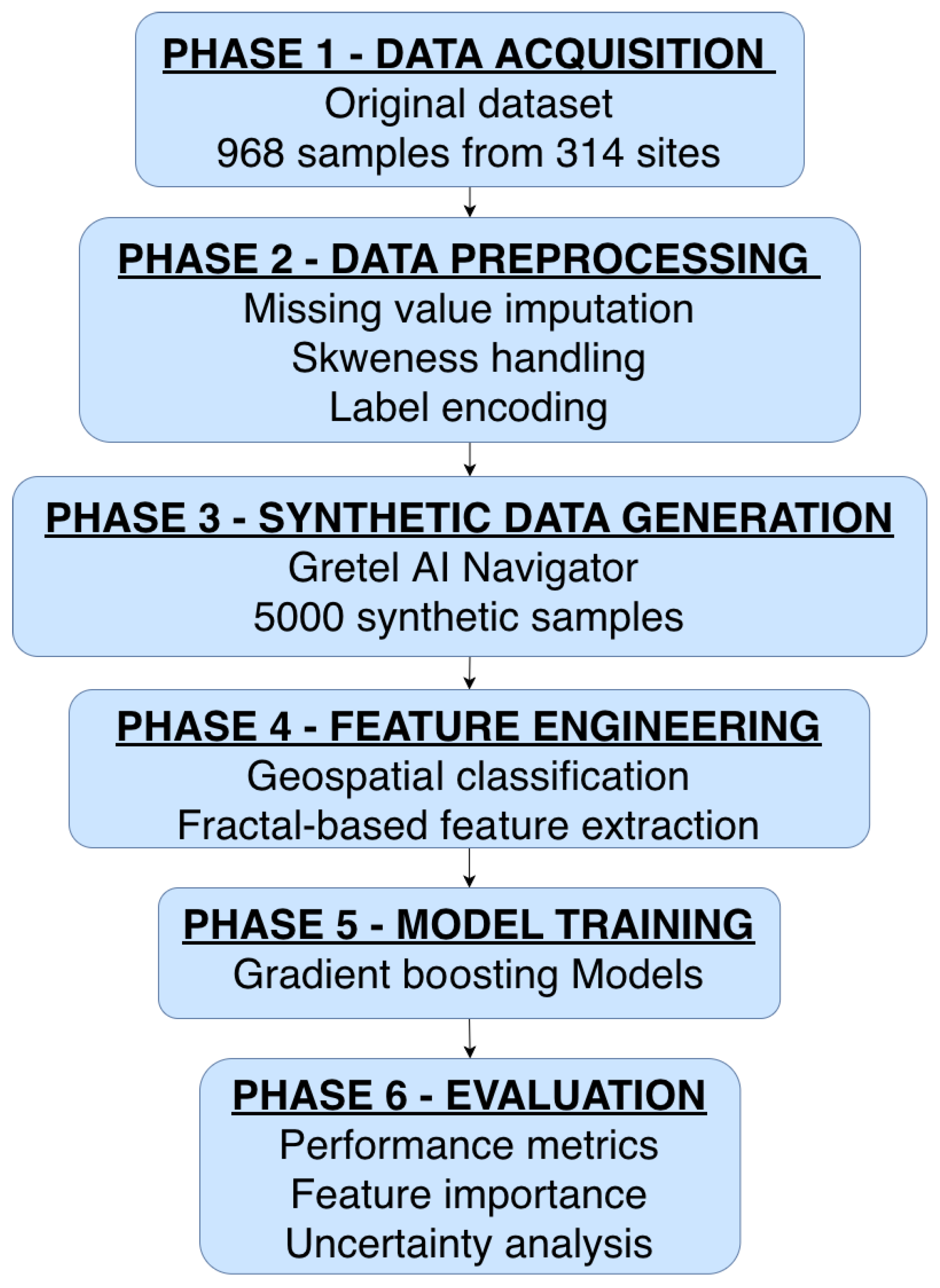
Hybrid Preprocessing and Augmented Boosting Framework (HPABF) for litterfall prediction. The framework illustrates the overall system architecture, including data acquisition from the original dataset and synthetic data generation, hybrid preprocessing and feature engineering with geospatial and fractal-based features, model training using multiple machine learning algorithms, and final evaluation through performance metrics, feature importance analysis, and uncertainty assessment.
Figure 1.
Hybrid Preprocessing and Augmented Boosting Framework (HPABF) for litterfall prediction. The framework illustrates the overall system architecture, including data acquisition from the original dataset and synthetic data generation, hybrid preprocessing and feature engineering with geospatial and fractal-based features, model training using multiple machine learning algorithms, and final evaluation through performance metrics, feature importance analysis, and uncertainty assessment.
Figure 2.
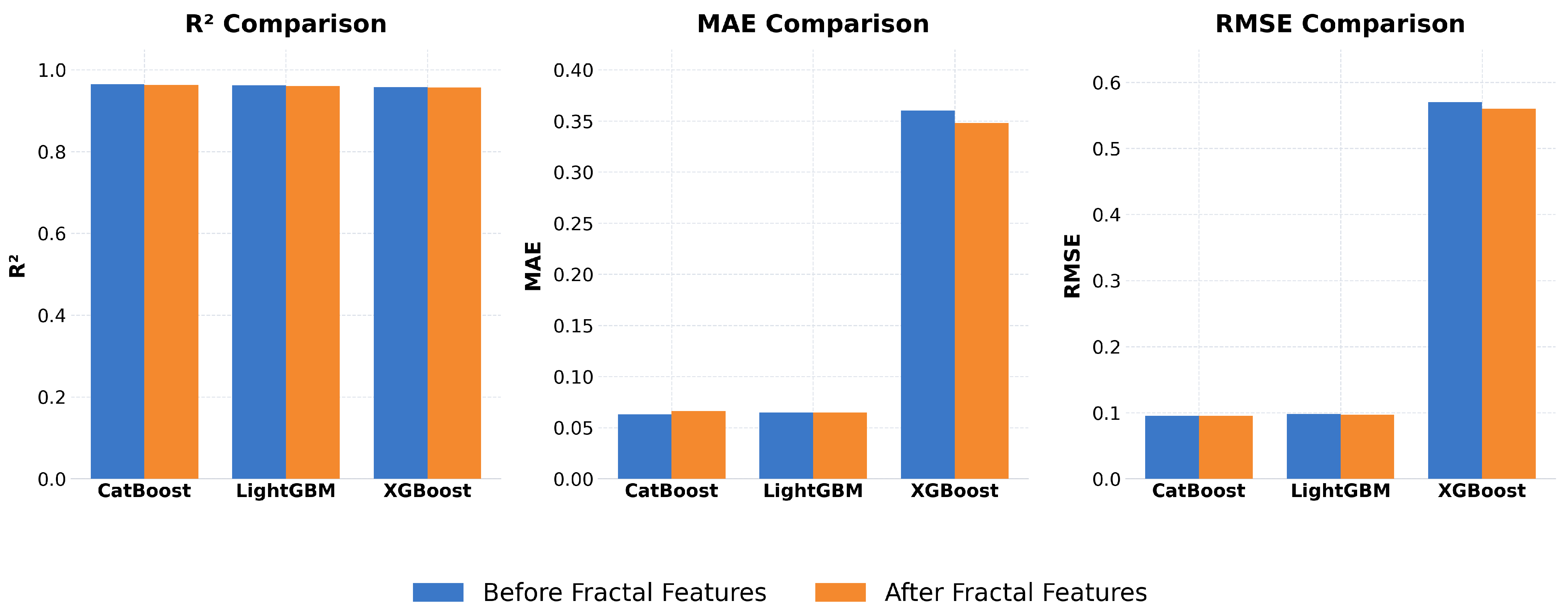
Comparison of model performance before and after incorporating fractal dimension features. The bar charts present the evaluation metrics R2, MAE, and RMSE for the CatBoost, LightGBM, and XGBoost models, illustrating the influence of fractal-based feature augmentation on predictive accuracy and error reduction.
Figure 2.
Comparison of model performance before and after incorporating fractal dimension features. The bar charts present the evaluation metrics R2, MAE, and RMSE for the CatBoost, LightGBM, and XGBoost models, illustrating the influence of fractal-based feature augmentation on predictive accuracy and error reduction.
Figure 3.
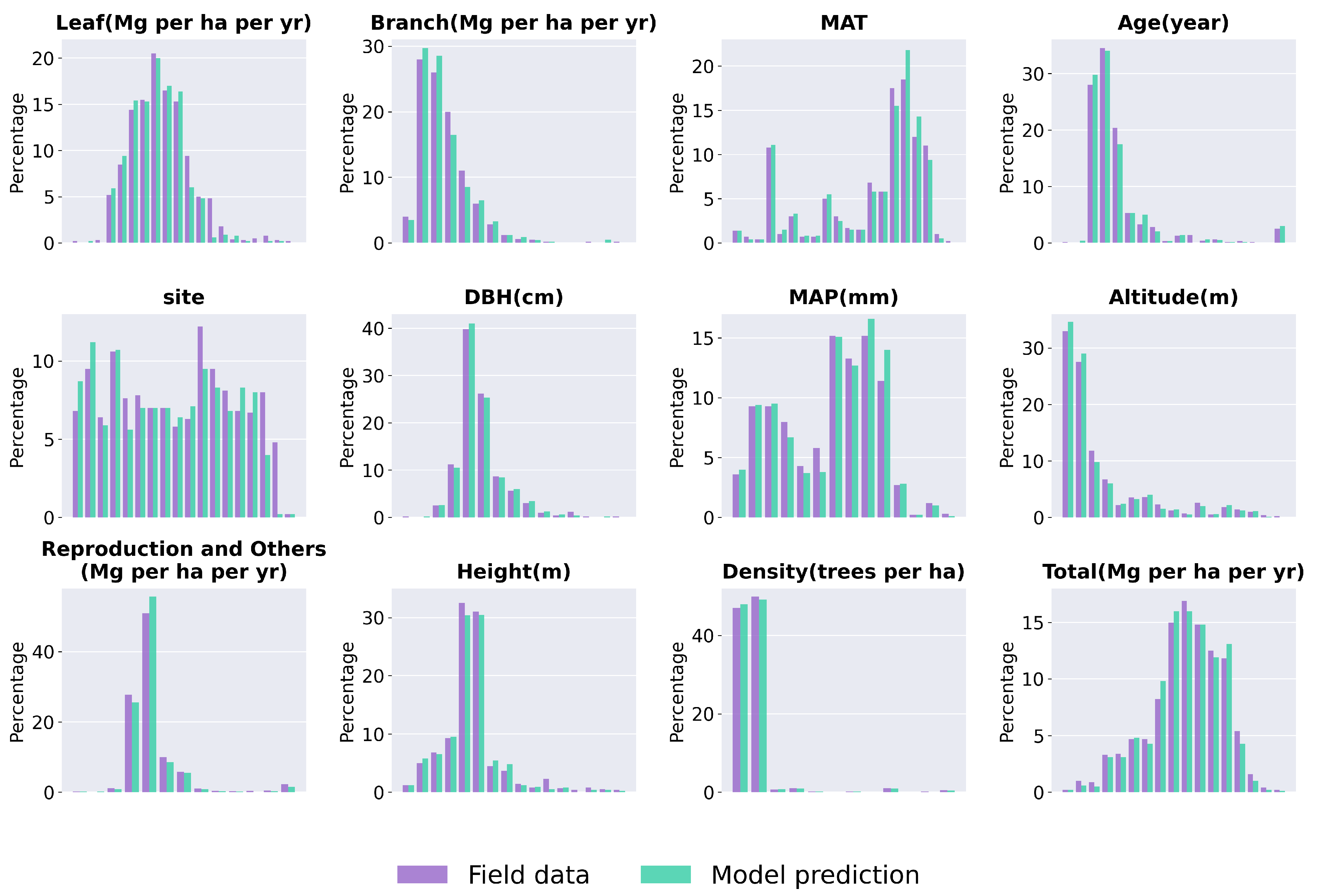
Distribution comparison of numerical litterfall-related features between observed field data (purple) and model predictions (teal), expressed as the percentage of observations per bin. The variables include biomass components (leaf, branch, reproduction and others, and total litterfall), stand structural attributes (DBH, height, age, and density), and environmental variables (MAT, MAP, altitude, and site). The overall similarity between the two distributions suggests that the model predictions closely reproduce the statistical characteristics of the observed field dataset.
Figure 3.
Distribution comparison of numerical litterfall-related features between observed field data (purple) and model predictions (teal), expressed as the percentage of observations per bin. The variables include biomass components (leaf, branch, reproduction and others, and total litterfall), stand structural attributes (DBH, height, age, and density), and environmental variables (MAT, MAP, altitude, and site). The overall similarity between the two distributions suggests that the model predictions closely reproduce the statistical characteristics of the observed field dataset.
Figure 4.
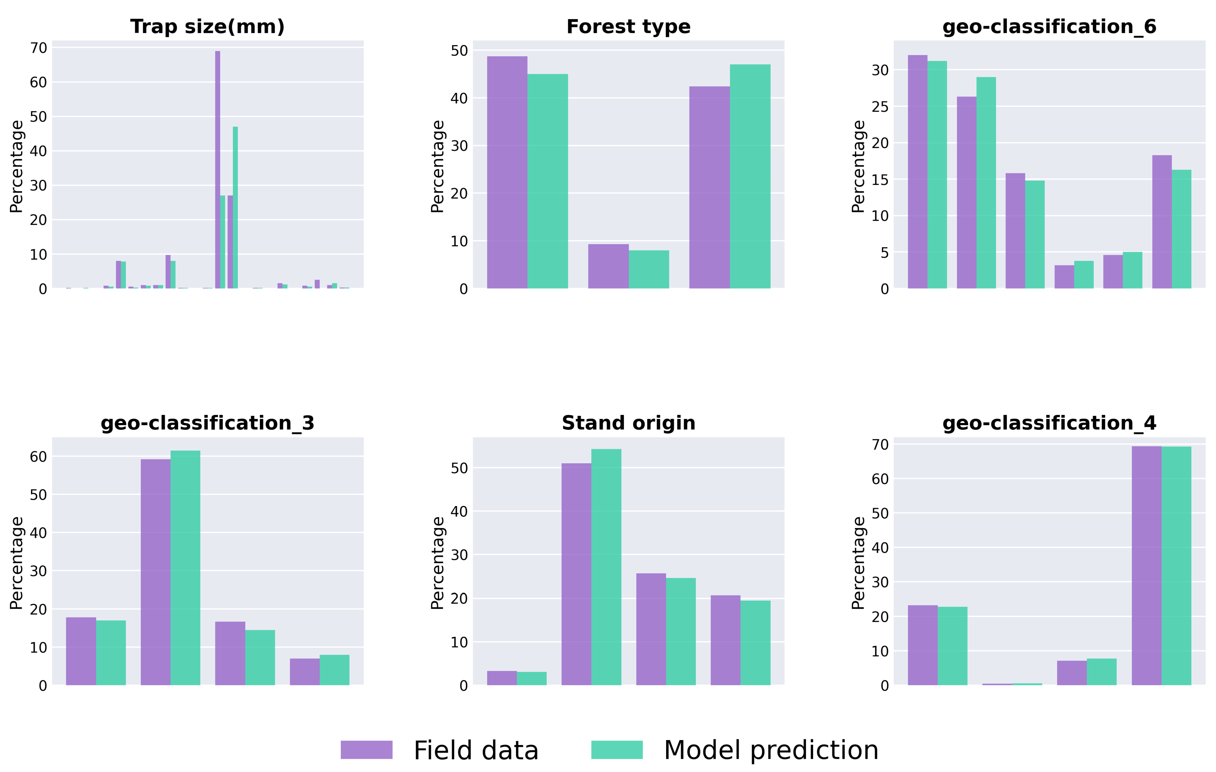
Distribution comparison of categorical variables between observed field data (purple) and model predictions (teal), expressed as the percentage of observations per category. The variables include forest type, stand origin, trap size (mm), and geo-classification variables. The close correspondence between observed and predicted class frequencies indicates that the model effectively preserves the categorical structure of the original dataset.
Figure 4.
Distribution comparison of categorical variables between observed field data (purple) and model predictions (teal), expressed as the percentage of observations per category. The variables include forest type, stand origin, trap size (mm), and geo-classification variables. The close correspondence between observed and predicted class frequencies indicates that the model effectively preserves the categorical structure of the original dataset.
Figure 5.
Comparison of the before vs. after for all three models in a grouped bar plot.
Figure 5.
Comparison of the before vs. after for all three models in a grouped bar plot.
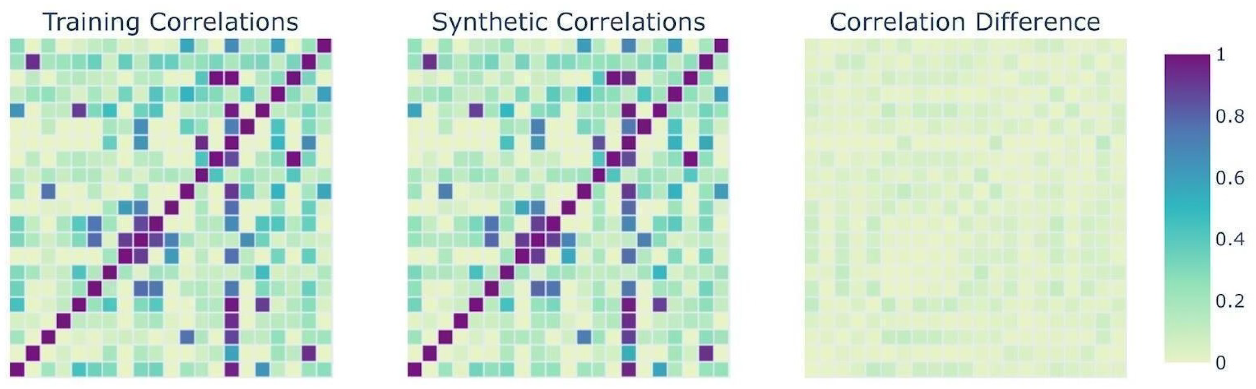
Figure 6.
Correlation heatmap for training and synthetic data generated by Gretel AI [
10].
Figure 6.
Correlation heatmap for training and synthetic data generated by Gretel AI [
10].
Table 1.
Comparative analysis of machine learning approaches relevant to forest biomass and litterfall prediction, with emphasis on gradient boosting and data augmentation strategies (2020–2026) (ordered by methodological relevance).
Table 1.
Comparative analysis of machine learning approaches relevant to forest biomass and litterfall prediction, with emphasis on gradient boosting and data augmentation strategies (2020–2026) (ordered by methodological relevance).
| Study | Models Used | Data Used | Key Findings | Strengths | Limitations |
|---|
| Guo et al. [7] | Transformer–CatBoost hybrid model | Multi-source climatic, remote sensing, and forest inventory data (China; 88 sites, monthly observations) | Spatiotemporal modeling improves litterfall prediction compared to single-model approaches | Captures temporal dynamics and nonlinear relationships | Requires large datasets; preprocessing strategies not systematically evaluated |
| Geng et al. [6] | LightGBM, XGBoost, Random Forest, linear models | Environmental and climatic variables from forest sites in China (968 samples) | Gradient boosting models outperform traditional and tree-based approaches for litterfall prediction | Strong benchmark for litterfall modeling; comprehensive model comparison | Limited data size; no synthetic data augmentation or systematic preprocessing analysis |
| Li et al. [14] | XGBoost with spatial correction (Kriging) | Landsat time series, forest inventory, climate scenarios (China) | Spatially enhanced gradient boosting improves biomass prediction | High predictive accuracy; accounts for spatial dependency | Complex pipeline; limited scalability assessment |
| Zhou et al. [4] | SVM, RF, XGBoost with multi-sensor fusion | Landsat, MODIS, topographic and meteorological data (China) | Gradient boosting outperforms traditional ML in biomass estimation | Effective multi-source integration | Generalization across forest types not fully assessed |
| Ali et al. [5] | RF, ANN, XGBoost ensembles | Sentinel-1/2, GEDI LiDAR, climate data (global forests) | Ensemble learning improves biomass estimation accuracy | Robust multi-model framework | High computational cost; preprocessing sensitivity underexplored |
| Li et al. [3] | Linear regression, RF, XGBoost | Landsat 8, Sentinel-1A SAR, national forest inventory (China) | Gradient boosting reduces bias compared to traditional models | Clear demonstration of boosting advantages | Limited regional scope; no data augmentation |
| Liu et al. [15] | RF and gradient boosting regression | Sentinel-2, Sentinel-1 SAR, environmental data (China) | Gradient boosting yields best biomass estimates | Highlights feature importance | SAR data degraded performance; moderate accuracy |
| Rafiq et al. [21] | GANs and VAEs for synthetic data | Review of ecological synthetic data applications | Synthetic data mitigates data scarcity | Conceptual support for augmentation | Lacks predictive validation |
| Bauer et al. [22] | GANs, diffusion models, transformers | Survey of synthetic data generation models | Neural generative models dominate SDG | Comprehensive methodological overview | Not forestry-specific |
| Wang et al. [12] | CNNs and LSTMs | Remote sensing, IoT, and climate data | Deep learning captures spatiotemporal forest dynamics | Strong temporal modeling | Requires large datasets |
| Aziz et al. [16] | RF, SVM, CNN | Landsat and Sentinel-2 data (Pakistan) | Deep learning improves forest cover classification | High classification accuracy | Not applicable to litterfall regression |
Table 2.
Description of variables included in the litterfall dataset.
Table 2.
Description of variables included in the litterfall dataset.
| Variable | Type | Description |
|---|
| Latitude | Numerical | Geographic latitude of the forest site |
| Longitude | Numerical | Geographic longitude of the forest site |
| Altitude | Numerical | Elevation of the site (m above sea level) |
| MAT | Numerical | Mean annual temperature (°C) |
| MAP | Numerical | Mean annual precipitation (mm) |
| Age | Numerical | Stand age (years) |
| DBH | Numerical | Diameter at breast height (cm) |
| Height | Numerical | Average tree height (m) |
| Density | Numerical | Tree density (trees per hectare) |
| Leaf | Numerical | Annual leaf litterfall (Mg ha−1 yr−1) |
| Branch | Numerical | Annual branch litterfall (Mg ha−1 yr−1) |
| Reproductive | Numerical | Litterfall from reproductive parts (Mg ha−1 yr−1) |
| Others | Numerical | Other litterfall components (Mg ha−1 yr−1) |
| Total | Numerical | Total annual litterfall production (Mg ha−1 yr−1) |
| Forest type | Categorical | Broadleaf, needleleaf, or mixed forest |
| Stand origin | Categorical | Natural or planted forest |
| Measurement interval | Categorical | Time interval of litterfall measurement |
| Trap size | Categorical | Size category of litter collection trap |
| Source | Categorical | Dataset source reference |
| Geospatial classification 1 | Categorical | Regional ecological classification level 1 |
| Geospatial classification 2 | Categorical | Regional ecological classification level 2 |
| Geospatial classification 3 | Categorical | Regional ecological classification level 3 |
Table 3.
Machine learning models used in this study.
Table 3.
Machine learning models used in this study.
| ML Model | Description |
|---|
| Linear Regression | Models linear relationships between features and litterfall [26]. |
| Ridge Regression | Adds an L2 regularization term to address multicollinearity [27]. |
| Decision Tree | Captures nonlinear interactions using hierarchical, threshold-based splits [28]. |
| LightGBM | Gradient boosting model with histogram-based splits and leaf-wise tree growth [29,30]. |
| CatBoost | Gradient boosting method designed to handle categorical variables efficiently. |
| XGBoost | Scalable ensemble boosting algorithm using optimized decision trees [12]. |
| Neural Network | Learns nonlinear patterns using multiple interconnected hidden layers [31]. |
| Random Forest | Combines multiple decision trees to improve predictive stability and reduce overfitting [32,33]. |
Table 4.
Key hyperparameters used for the machine learning models.
Table 4.
Key hyperparameters used for the machine learning models.
| Model | Key Hyperparameters |
|---|
| Linear Regression | Default parameters |
| Ridge Regression | alpha = 1.0 |
| Decision Tree | random_state = 42 |
| LightGBM | n_estimators = 100, random_state = 42 |
| CatBoost | iterations = 100, random_state = 42 |
| XGBoost | n_estimators = 3000, learning_rate = 0.1, max_depth = 2, early_stopping_rounds = 20, eval_metric = RMSE |
| Neural Network | hidden layers = (64, 32, 16), activation = ReLU, optimizer = Adam, epochs = 50, batch size = 32 |
| Random Forest | n_estimators = 100, random_state = 42 |
Table 5.
Evaluation measures used to assess model performance.
Table 5.
Evaluation measures used to assess model performance.
| Measure | Description |
|---|
| R-squared (R2) | Proportion of variance in the target variable explained by the model; higher values indicate better fit. |
| Mean Absolute Error (MAE) | Average absolute difference between predicted and actual values; lower MAE denotes higher accuracy. |
| Root-Mean-Square Error (RMSE) | Square root of the average squared differences between predicted and actual values; lower RMSE indicates better predictive performance. |
| 2D Spatial Fractal Dimension | Captures spatial complexity based on latitude, longitude, and the target variable; higher values indicate greater spatial irregularity. |
| 3D Spatial Fractal Dimension | Measures spatial complexity including elevation (latitude, longitude, altitude, target); useful for altitude-dependent spatial patterns. |
| 3D Structural Fractal Dimension | Reflects structural complexity in vegetation attributes (e.g., DBH, height, density, target); indicates how well structural patterns are represented. |
Table 6.
Preprocessing scenarios applied to different geospatial classes.
Table 6.
Preprocessing scenarios applied to different geospatial classes.
| Scenario | Preprocessing Steps | Trial No. | Geospatial Class |
|---|
| Scenario 1 | Log transformation, drop columns with >25% nulls, then impute the remaining using MICE. | 3 | None |
| Scenario 2 | Same as Scenario 1. | 3 | Geo3 |
| Scenario 3 | Same as Scenario 1. | 3 | Geo4 |
| Scenario 4 | Same as Scenario 1. | 3 | Geo6 |
| Scenario 5 | Log transformation, then impute missing values using MICE. | 2 | None |
| Scenario 6 | Same as Scenario 5. | 2 | Geo3 |
| Scenario 7 | Same as Scenario 5. | 2 | Geo4 |
| Scenario 8 | Same as Scenario 5. | 2 | Geo6 |
| Scenario 9 | Use MICE and mode imputation directly to handle missing values. | 1 | None |
| Scenario 10 | Same as Scenario 9. | 1 | Geo3 |
| Scenario 11 | Same as Scenario 9. | 1 | Geo4 |
| Scenario 12 | Same as Scenario 9. | 1 | Geo6 |
Table 7.
R-squared values of the implemented algorithms across 12 preprocessing scenarios.
Table 7.
R-squared values of the implemented algorithms across 12 preprocessing scenarios.
| Scenario | Random Forest | Light GBM | CatBoost | Linear Regression | Ridge Regression | Decision Tree | XGBoost | Neural Net |
|---|
| Scenario 1 | 0.9577 | 0.9617 | 0.9632 | 0.8925 | 0.8925 | 0.9211 | 0.9602 | 0.9263 |
| Scenario 2 | 0.9560 | 0.9607 | 0.9604 | 0.8881 | 0.8881 | 0.9080 | 0.9599 | 0.9246 |
| Scenario 3 | 0.9570 | 0.9613 | 0.9619 | 0.8915 | 0.8915 | 0.9149 | 0.9598 | 0.9210 |
| Scenario 4 | 0.9563 | 0.9609 | 0.9614 | 0.8917 | 0.8917 | 0.9146 | 0.9591 | 0.9291 |
| Scenario 5 | 0.9550 | 0.9601 | 0.9556 | 0.8939 | 0.8939 | 0.9130 | 0.9548 | 0.9068 |
| Scenario 6 | 0.9533 | 0.9604 | 0.9546 | 0.8917 | 0.8917 | 0.9109 | 0.9564 | 0.9052 |
| Scenario 7 | 0.9543 | 0.9601 | 0.9582 | 0.8934 | 0.8934 | 0.9147 | 0.9552 | 0.9137 |
| Scenario 8 | 0.9545 | 0.9589 | 0.9569 | 0.8938 | 0.8938 | 0.9188 | 0.9549 | 0.9122 |
| Scenario 9 | 0.9452 | 0.9504 | 0.9526 | 0.9526 | 0.9526 | 0.8999 | 0.9548 | 0.9423 |
| Scenario 10 | 0.9435 | 0.9468 | 0.9457 | 0.9519 | 0.9519 | 0.8939 | 0.9537 | 0.9483 |
| Scenario 11 | 0.9435 | 0.9472 | 0.9448 | 0.9522 | 0.9522 | 0.8991 | 0.9546 | 0.9470 |
| Scenario 12 | 0.9445 | 0.9481 | 0.9482 | 0.9525 | 0.9525 | 0.8962 | 0.9531 | 0.9455 |
Table 8.
Root-Mean-Square Error (RMSE) values of the implemented algorithms across 12 preprocessing scenarios.
Table 8.
Root-Mean-Square Error (RMSE) values of the implemented algorithms across 12 preprocessing scenarios.
| Scenario | Random Forest | Light GBM | CatBoost | Linear Regression | Ridge Regression | Decision Tree | XGBoost | Neural Net |
|---|
| Scenario 1 | 0.0953 | 0.0907 | 0.0896 | 0.1529 | 0.1529 | 0.1303 | 0.0929 | 0.1250 |
| Scenario 2 | 0.0972 | 0.0920 | 0.0928 | 0.1560 | 0.1560 | 0.1405 | 0.0932 | 0.1269 |
| Scenario 3 | 0.0960 | 0.0912 | 0.0911 | 0.1537 | 0.1537 | 0.1344 | 0.0936 | 0.1282 |
| Scenario 4 | 0.0968 | 0.0918 | 0.0913 | 0.1535 | 0.1535 | 0.1354 | 0.0941 | 0.1208 |
| Scenario 5 | 0.0984 | 0.0925 | 0.0986 | 0.1519 | 0.1519 | 0.1364 | 0.0987 | 0.1391 |
| Scenario 6 | 0.1001 | 0.0921 | 0.0990 | 0.1535 | 0.1535 | 0.1384 | 0.0971 | 0.1427 |
| Scenario 7 | 0.0991 | 0.0923 | 0.0945 | 0.1523 | 0.1523 | 0.1358 | 0.0986 | 0.1366 |
| Scenario 8 | 0.0989 | 0.0937 | 0.0966 | 0.1520 | 0.1520 | 0.1331 | 0.0988 | 0.1366 |
| Scenario 9 | 0.6151 | 0.5872 | 0.5881 | 0.5722 | 0.5722 | 0.8170 | 0.5594 | 0.6355 |
| Scenario 10 | 0.6251 | 0.6088 | 0.6163 | 0.5764 | 0.5764 | 0.8616 | 0.5663 | 0.6020 |
| Scenario 11 | 0.6245 | 0.6074 | 0.6202 | 0.5742 | 0.5742 | 0.8400 | 0.5604 | 0.6082 |
| Scenario 12 | 0.6192 | 0.6016 | 0.6015 | 0.5726 | 0.5726 | 0.8479 | 0.5707 | 0.6137 |
Table 9.
Mean Absolute Error (MAE) values of the implemented algorithms across 12 preprocessing scenarios.
Table 9.
Mean Absolute Error (MAE) values of the implemented algorithms across 12 preprocessing scenarios.
| Scenario | Random Forest | LightGBM | CatBoost | Linear Regression | Ridge Regression | Decision Tree | XGBoost | Neural Net |
|---|
| Scenario 1 | 0.0681 | 0.0646 | 0.0631 | 0.1061 | 0.1061 | 0.0939 | 0.0672 | 0.0891 |
| Scenario 2 | 0.0702 | 0.0660 | 0.0670 | 0.1092 | 0.1092 | 0.0989 | 0.0672 | 0.0894 |
| Scenario 3 | 0.0689 | 0.0650 | 0.0658 | 0.1075 | 0.1075 | 0.0979 | 0.0674 | 0.0901 |
| Scenario 4 | 0.0692 | 0.0656 | 0.0654 | 0.1075 | 0.1075 | 0.0979 | 0.0676 | 0.0849 |
| Scenario 5 | 0.0698 | 0.0642 | 0.0681 | 0.1042 | 0.1042 | 0.0957 | 0.0703 | 0.0956 |
| Scenario 6 | 0.0711 | 0.0652 | 0.0688 | 0.1061 | 0.1061 | 0.0969 | 0.0701 | 0.1002 |
| Scenario 7 | 0.0702 | 0.0649 | 0.0656 | 0.1047 | 0.1047 | 0.0943 | 0.0709 | 0.0955 |
| Scenario 8 | 0.0700 | 0.0654 | 0.0680 | 0.1049 | 0.1049 | 0.0955 | 0.0709 | 0.0947 |
| Scenario 9 | 0.3829 | 0.3602 | 0.3721 | 0.3662 | 0.3664 | 0.5298 | 0.3596 | 0.4106 |
| Scenario 10 | 0.3883 | 0.3731 | 0.3847 | 0.3643 | 0.3646 | 0.5467 | 0.3605 | 0.4070 |
| Scenario 11 | 0.3881 | 0.3744 | 0.3852 | 0.3628 | 0.3631 | 0.5362 | 0.3597 | 0.3927 |
| Scenario 12 | 0.3855 | 0.3693 | 0.3875 | 0.3644 | 0.3646 | 0.5373 | 0.3651 | 0.4112 |
Table 10.
Samples with the largest prediction errors across the evaluated models.
Table 10.
Samples with the largest prediction errors across the evaluated models.
| Sample ID | True Value | LightGBM | CatBoost | XGBoost | Largest Error |
|---|
| 764 | 2.7389 | 13.6404 | 14.9915 | 2.36 | 12.2526 |
| 874 | 2.6025 | 13.5081 | 13.2418 | 2.24 | 10.6393 |
| 280 | 2.7846 | 13.6411 | 13.3204 | 2.35 | 10.5358 |
Table 11.
Data scarcity test: model performance under reduced training fractions using 10-fold cross-validation.
Table 11.
Data scarcity test: model performance under reduced training fractions using 10-fold cross-validation.
| Model | Training Fraction | R2 | MAE | RMSE |
|---|
| XGBoost | 50% | 0.954 | 0.071 | 0.100 |
| | 25% | 0.942 | 0.080 | 0.111 |
| | 10% | 0.918 | 0.095 | 0.132 |
| CatBoost | 50% | 0.951 | 0.075 | 0.103 |
| | 25% | 0.935 | 0.083 | 0.119 |
| | 10% | 0.882 | 0.111 | 0.160 |
| LightGBM | 50% | 0.947 | 0.075 | 0.107 |
| | 25% | 0.918 | 0.092 | 0.133 |
| | 10% | 0.824 | 0.145 | 0.196 |
Table 12.
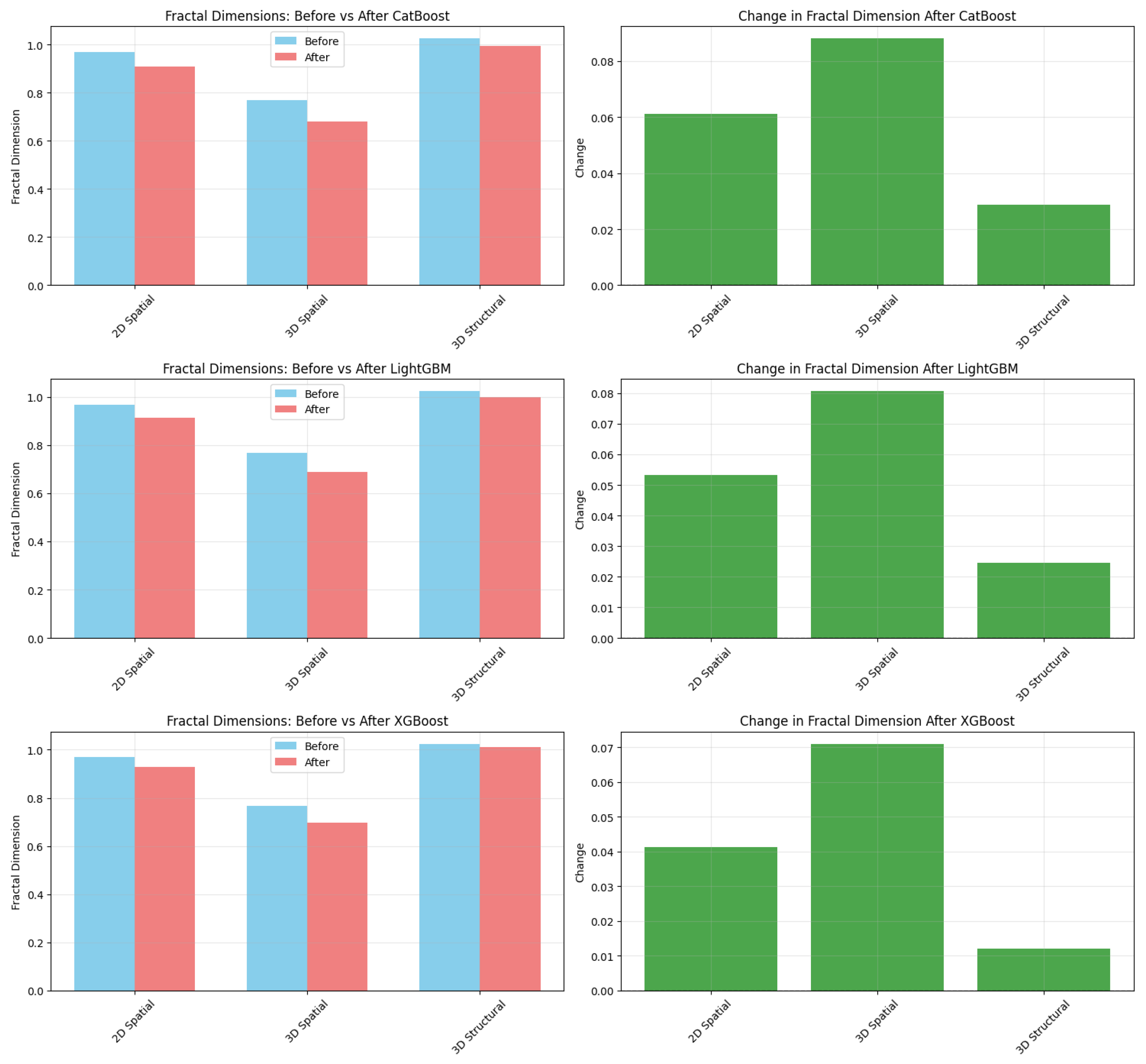
Fractal dimension analysis before and after CatBoost for Scenario 1, processing Trial 3.
Table 12.
Fractal dimension analysis before and after CatBoost for Scenario 1, processing Trial 3.
| Fractal Metric | Before CatBoost | After CatBoost | Change | % Change |
|---|
| 2D Spatial (Lat, Lon + Target) | 0.9684 | 0.9272 | −0.0412 | −4.25% |
| 3D Spatial (Lat, Lon, Alt + Target) | 0.7678 | 0.6968 | −0.0710 | −9.25% |
| 3D Structural (DBH, Height, Density+ Target) | 1.0242 | 1.0121 | −0.0121 | −1.18% |
Table 13.
Fractal dimension analysis before and after LightGBM for Scenario 6, processing Trial 2.
Table 13.
Fractal dimension analysis before and after LightGBM for Scenario 6, processing Trial 2.
| Fractal Metric | Before LightGBM | After LightGBM | Change | % Change |
|---|
| 2D Spatial (Lat, Lon + Target) | 0.9684 | 0.9072 | −0.0611 | −6.31% |
| 3D Spatial (Lat, Lon, Alt + Target) | 0.7678 | 0.6798 | −0.0880 | −11.46% |
| 3D Structural (DBH, Height, Density + Target) | 1.0242 | 0.9954 | −0.0288 | −2.81% |
Table 14.
Fractal dimension analysis before and after XGBoost for Scenario 9, processing Trial 1.
Table 14.
Fractal dimension analysis before and after XGBoost for Scenario 9, processing Trial 1.
| Fractal Metric | Before XGBoost | After XGBoost | Change | % Change |
|---|
| 2D Spatial (Lat, Lon + Target) | 0.9684 | 0.9152 | −0.0532 | −5.49% |
| 3D Spatial (Lat, Lon, Alt + Target) | 0.7678 | 0.6871 | −0.0807 | −10.51% |
| 3D Structural (DBH, Height, Density + Target) | 1.0242 | 0.9997 | −0.0244 | −2.39% |
Table 15.
R-squared values of algorithms on synthetic data across Scenarios S5 to S8.
Table 15.
R-squared values of algorithms on synthetic data across Scenarios S5 to S8.
| Algorithm | S5 | S6 | S7 | S8 |
|---|
| Random Forest | 0.9832 | 0.9819 | 0.9821 | 0.9821 |
| LightGBM | 0.9828 | 0.9819 | 0.9821 | 0.9818 |
| CatBoost | 0.9817 | 0.9795 | 0.9792 | 0.9788 |
| Linear Reg. | 0.8970 | 0.8333 | 0.8333 | 0.8336 |
| Ridge Reg. | 0.8970 | 0.8333 | 0.8333 | 0.8336 |
| Decision Tree | 0.9714 | 0.9670 | 0.9840 | 0.9692 |
| XGBoost | 0.9791 | 0.9781 | 0.9777 | 0.9786 |
| Neural Net | 0.9695 | 0.9611 | 0.9587 | 0.9633 |
Table 16.
Root-Mean-Square Error (RMSE) of algorithms on synthetic data across Scenarios S5 to S8.
Table 16.
Root-Mean-Square Error (RMSE) of algorithms on synthetic data across Scenarios S5 to S8.
| Algorithm | S5 | S6 | S7 | S8 |
|---|
| Random Forest | 0.0611 | 0.0256 | 0.0255 | 0.0255 |
| LightGBM | 0.0620 | 0.0257 | 0.0256 | 0.0258 |
| CatBoost | 0.0640 | 0.0274 | 0.0276 | 0.0278 |
| Linear Reg. | 0.1524 | 0.0786 | 0.0786 | 0.0785 |
| Ridge Reg. | 0.1524 | 0.0786 | 0.0786 | 0.0785 |
| Decision Tree | 0.0800 | 0.0348 | 0.0340 | 0.0336 |
| XGBoost | 0.0684 | 0.0284 | 0.0286 | 0.0280 |
| Neural Net | 0.0827 | 0.0379 | 0.0389 | 0.0367 |
Table 17.
Mean Absolute Error (MAE) of algorithms on synthetic data across Scenarios S5 to S8.
Table 17.
Mean Absolute Error (MAE) of algorithms on synthetic data across Scenarios S5 to S8.
| Algorithm | S5 | S6 | S7 | S8 |
|---|
| Random Forest | 0.0301 | 0.0117 | 0.0117 | 0.0117 |
| LightGBM | 0.0361 | 0.0142 | 0.0141 | 0.0143 |
| CatBoost | 0.0403 | 0.0159 | 0.0159 | 0.0160 |
| Linear Reg. | 0.1045 | 0.0514 | 0.0514 | 0.0514 |
| Ridge Reg. | 0.1045 | 0.0514 | 0.0514 | 0.0514 |
| Decision Tree | 0.0359 | 0.0140 | 0.0138 | 0.0139 |
| XGBoost | 0.0442 | 0.0176 | 0.0180 | 0.0173 |
| Neural Net | 0.0547 | 0.0244 | 0.0238 | 0.0240 |
Table 18.
R-squared values for the best-performing algorithm and preprocessing trial in each scenario.
Table 18.
R-squared values for the best-performing algorithm and preprocessing trial in each scenario.
| Scenario | Preprocessing Trial | Best Algorithm (R2) | Training Time |
|---|
| Scenario 1 | 3 | CatBoost: 0.9632 | 2.35 s |
| Scenario 2 | 3 | LightGBM: 0.9607 | 0.81 s |
| Scenario 3 | 3 | LightGBM: 0.9613 | 0.8 s |
| Scenario 4 | 3 | CatBoost: 0.9614 | 2.1 s |
| Scenario 5 | 2 | LightGBM: 0.9601 | 1.26 s |
| Scenario 6 | 2 | LightGBM: 0.9604 | 1.15 s |
| Scenario 7 | 2 | LightGBM: 0.9601 | 1.17 s |
| Scenario 8 | 2 | LightGBM: 0.9589 | 1.17 s |
| Scenario 9 | 1 | XGBoost: 0.9548 | 2.69 s |
| Scenario 10 | 1 | XGBoost: 0.9537 | 1.9 s |
| Scenario 11 | 1 | XGBoost: 0.9546 | 1.6 s |
| Scenario 12 | 1 | XGBoost: 0.9531 | 1.6 s |