Scenario-Based Stochastic Optimization for Long-Term Scheduling of Hydro–Wind–Solar Complementary Energy Systems

Abstract

As the global energy transition accelerates, clean energy development has surged. However, accurately modeling correlations and uncertainties of hydro, wind, and photovoltaic energy remains challenging in long-term scheduling for energy complementarity. This study employs Latin hypercube sampling and Cholesky decomposition to capture the temporal correlations of water runoff, wind, and photovoltaic resources. It generates numerous scenarios for uncertainty simulation. The scenario set is reduced based on probability distance while maintaining a high-fidelity approximation. A stochastic dual-objective model is proposed for long-term multi-energy complementary system scheduling (LMCS), aiming to maximize expected revenue considering carbon emission costs while ensuring minimum power output guarantees. An evolutionary algorithm—namely, an orthogonal multi-population evolutionary (OMPE) algorithm based on orthogonal design and a multi-population search framework—is introduced, along with constraint-handling strategies. Three annual-regulation hydropower stations in the Hongshui River Basin serve as a case study. The experimental results indicate that generated scenarios capture temporal characteristics with high accuracy. The proposed algorithm efficiently solves the LMCS problem, achieving average increases of 5.46% and 3.89% in revenue and minimal output compared to benchmarks. The validation results demonstrate that orthogonalization-based initialization, recombination operators, and dominance rules significantly enhance OMPE performance. Sensitivity analysis indicates that economic efficiency and risk trade-offs can be adjusted by varying scenario numbers.

1. Introduction

In the coming decades, wind, photovoltaic (PV), and hydropower are anticipated to shape the global energy landscape, as indicated by the International Energy Agency (IEA) [1]. However, the volatility and intermittency of wind and PV power generation complicate the scheduling of these resources within the power system. Improving the efficiency, stability, and economic performance of power systems in the parallel scheduling of hydropower, wind, and PV energy has thus become a key research focus in the field of energy scheduling. Among existing multi-energy complementary approaches, hydro-PV combinations [2] and hydro–wind–PV complementary systems [3] are widely applied. This study will focus on the operational scheduling of hydro–wind–PV complementary systems.

Currently, regarding the operational planning of multi-energy complementary systems, scholars have made substantial progress in short-term coordination optimization [4,5], particularly in (i) characterizing uncertainties in hydropower, wind, and solar power, (ii) improving short-term generation prediction, (iii) constructing mathematical models for problem representation, and (iv) designing high-performance solving algorithms [6]. Y. Singh et al. [7] proposed an improved control method based on complex variable filters. It enhances the power quality performance of wind–solar complementary and battery-based microgrids under weak-grid and dynamic-load conditions. Wu et al. [8] introduced a Gaussian mixture model (GMM)-based framework to address cumulative renewable generation errors in short-term scheduling, quantifying multi-period deviation distributions and boundary constraints to optimize hydropower reserve allocation in cascaded systems. Li et al. [9] developed a deep learning-driven stochastic scheduling model coupled with a nested PSO-DP algorithm, targeting renewable intermittency through multi-energy synergy optimization and cascaded hydropower regulation, validated in a national renewable energy base. These approaches collectively advance scalable solutions for balancing renewable variability while improving operational efficiency and grid resilience in short-term hybrid energy systems. Regarding uncertainty characterization, Wang et al. [10] represented the output errors of wind and PV power using Gaussian distributions. Later, Xiong et al. [11] further employed probabilistic models to describe the generation deviations caused by misalignment of wind and PV power outputs across multiple consecutive time periods, thus enhancing the accuracy of uncertainty characterization for wind and PV energy. Zheng et al. 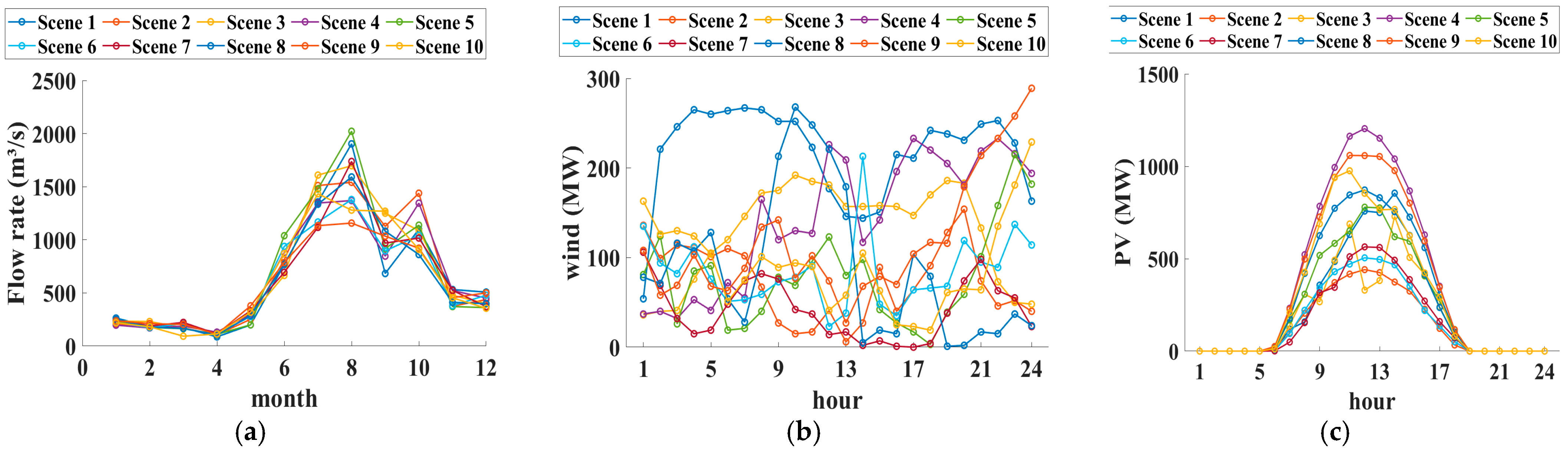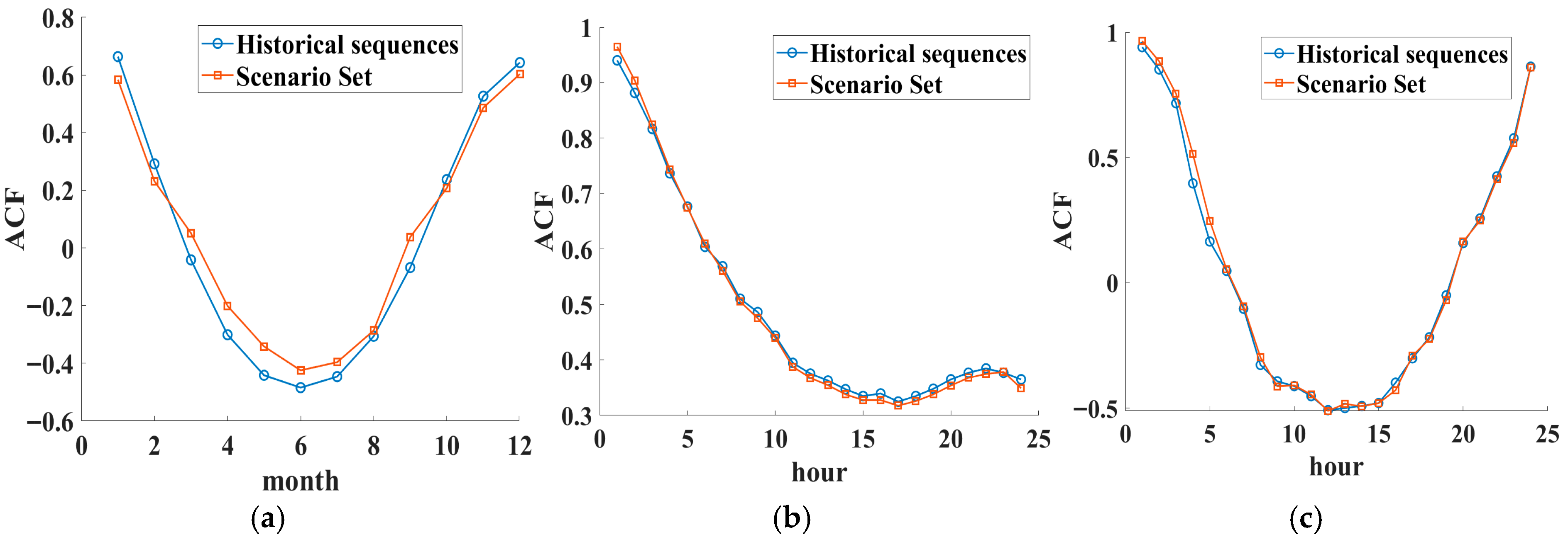[12] combined the martingale model of forecast evolution (MMFE) with the neural gas method to simulate uncertainty and its evolution process in the form of a comprehensive ensemble forecast and then converted it into a scenario tree. In reality, the output of hydro, wind, and PV energy shows significant uncertainty due to seasonal variations. However, the aforementioned studies did not consider the temporal correlation between resources. Latin hypercube sampling (LHS) effectively reflects the overall distribution of random variables. In this study, LHS simulation is used to generate scenarios of hydro, wind, and PV resources, while Cholesky decomposition is applied to reduce the correlation between multiple independent input random variable sampling values [13,14]. The computational complexity of scenario-based stochastic optimization problems primarily depends on the number of scenarios. However, probability distance-based scenario elimination enables a high-fidelity approximation of the initial scenario set while maintaining computational feasibility [15]. Various advanced uncertainty quantification techniques, such as approximate Bayesian computation, have also been explored in other engineering domains [16]. Therefore, this study will explore the temporal correlations between hydro and wind–PV resources using this approach, aiming to better characterize the multiple uncertainties inherent in these resources and establish a strong foundation for subsequent model development.

Research on the long-term multi-energy complementary system scheduling (LMCS) is relatively limited, making it an emerging area of interest in recent years. Because wind and solar power are non-dispatchable, most related studies have focused on integrating renewable energy sources, such as wind and PV, as boundary conditions within traditional hydropower scheduling frameworks, leading to valuable explorations. For example, multi-objective scheduling optimization for medium- and long-term periods has been studied [17]. This study will focus on the aspect of multi-objective scheduling optimization for medium- and long-term periods. Current research on single-objective optimization for LMCS involves objective functions such as maximizing total power generation [18], minimizing output volatility [19], and ensuring guaranteed output levels [20], among others. Moreover, reliance solely on generation volume overlooks the economic implications of environmental footprints. To address this, recent studies have begun to integrate carbon emission costs into the objective function, utilizing full life-cycle carbon emission factors and market-based carbon pricing to quantify environmental externalities [21]. Consequently, the optimization paradigm shifts from simply maximizing total electricity generation to maximizing the comprehensive total revenue, where carbon costs serve as a penalty term to incentivize low-carbon operational strategies [22]. However, scheduling solutions obtained using traditional single-objective optimization methods often struggle to maintain optimal performance in other objectives, especially when objectives conflict or are mutually exclusive. In contrast, multi-objective optimization methods for reservoir scheduling provide results that more objectively reflect the satisfaction of each objective, thereby more accurately revealing the extensive benefits of the reservoir and the decision preferences of each scheduling plan across various objectives. Multi-objective optimization is not just about solving a single-objective function; it requires finding a suitable balance between multiple conflicting objectives. For example, there may be a conflict between maximizing power generation and minimizing the minimum output level during specific time periods [23]. Key issues in scheduling optimization include how to reduce energy waste and improve the utilization of renewable energy while ensuring the stable operation of the system [24,25]. Other objectives include minimizing the load tracking deviation index or minimizing the total volume of water wasted during the scheduling period [26]. Multi-objective optimization frameworks can be categorized based on the temporal integration of decision preferences relative to the solution process [27]. Classical taxonomies distinguish (i) a priori methods requiring predetermined preference parameters (e.g., lexicographic ordering, scalarization functions), (ii) interactive preference refinement, and (iii) a posteriori Pareto-frontier generation. Priori techniques dominate practical implementations, while their reliance on accurate weight specification often introduces subjectivity biases, particularly in ill-defined preference spaces [28]. To circumvent this limitation, multi-objective optimization models are typically solved using multi-objective algorithms that generate a Pareto optimal solution set, alleviating the effort of decision makers. For instance, Dai et al. [29] proposed using the NSGA-II algorithm to solve the multi-objective optimization scheduling problem for reservoir groups. The scheduling results indicated that this method could achieve satisfactory outcomes, with the solutions uniformly covering the multi-objective optimal frontier within the solution space, thus providing sufficient decision-making information for decision makers. Similarly, Meng et al. [30] introduced a population initialization strategy based on constraint transformation into the multi-objective cuckoo search algorithm, presenting an improved multi-objective cuckoo search algorithm (IMOCS) [31]. By utilizing a hybrid microgrid system that combines wind–solar complementarity and electric hydrogen coupling, a dual-layer model of the microgrid is established, and an IGWO algorithm with excellent global performance is proposed for solving it, effectively improving the independence and stability of the microgrid and significantly reducing overall costs. Ji, B et al. [32] constructed an evolutionary multi-objective optimization algorithm driven by spatiotemporal coupling. After generating spatiotemporal correlated scenes through the joint Markov chain and Copula distributions, a dual population collaborative evolution mechanism with multiple recombination sub-fusion was designed, and heuristic constraint repair strategies to handle complex hydraulic coupling constraints were integrated. The aforementioned studies did not address channel constraints, and we will further explore the impact of such constraints.

Overall, significant and valuable progress has been made in the research on medium- and long-term multi-energy complementary scheduling problems abroad. However, multiple pivotal concerns remain outstanding, including the treatment of inter-resource dependencies in mid-/long-term multi-energy system coordination and how to account for the influence of channel constraints on model development. Therefore, this paper presents an integrated optimization framework for the long-term multi-energy complementary scheduling (LMCS) problem. This framework incorporates both multi-objective optimization and uncertainty analysis. The main contributions of this study are threefold.

First, unlike the approach used by Liu, W et al. [33], this study employs Latin hypercube sampling combined with Cholesky decomposition. This method addresses the limitations of existing uncertainty modeling approaches. Specifically, this module preserves the empirical distributions and temporal cross-correlations among the three energy sources within a unified framework. It thus provides a more realistic representation of multi-scale uncertainties.

Second, we recognize that generic multi-objective evolutionary algorithms do not explicitly account for the complex hydraulic coupling and water balance constraints in cascaded reservoir systems. Recent studies have demonstrated that adaptive multi-operator recombination and constraint-handling techniques can effectively address such challenges in complex scheduling problems [34,35]. Inspired by these successes, we develop an orthogonal multi-population evolutionary (OMPE) algorithm with problem-specific enhancements. These enhancements include three aspects:

(i) It uses an orthogonal design to initialize the population. This achieves systematic coverage of the high-dimensional solution space through symmetric discretization and orthogonal array construction. It also avoids clustering bias caused by random sampling.

(ii) It designs an adaptive recombination operator pool. This pool dynamically selects the optimal operator based on historical performance, thereby improving the algorithm’s robustness to different scenarios.

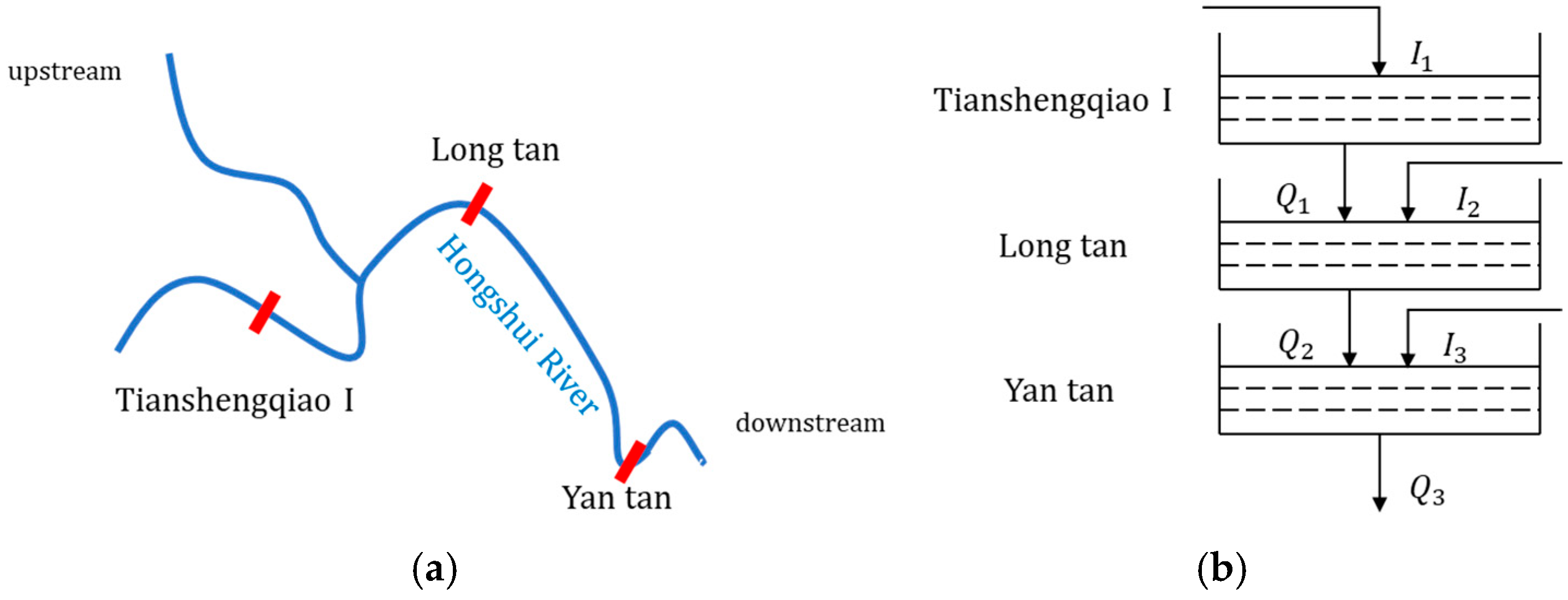
(iii) It adopts an ε-Box dominance rule combined with a heuristic constraint-handling strategy. This helps maintain feasibility under water balance and transmission limits. Third, we conduct a comprehensive evaluation of the proposed framework. The evaluation is carried out on three cascaded annual-regulation hydropower stations in the Hongshui River Basin.

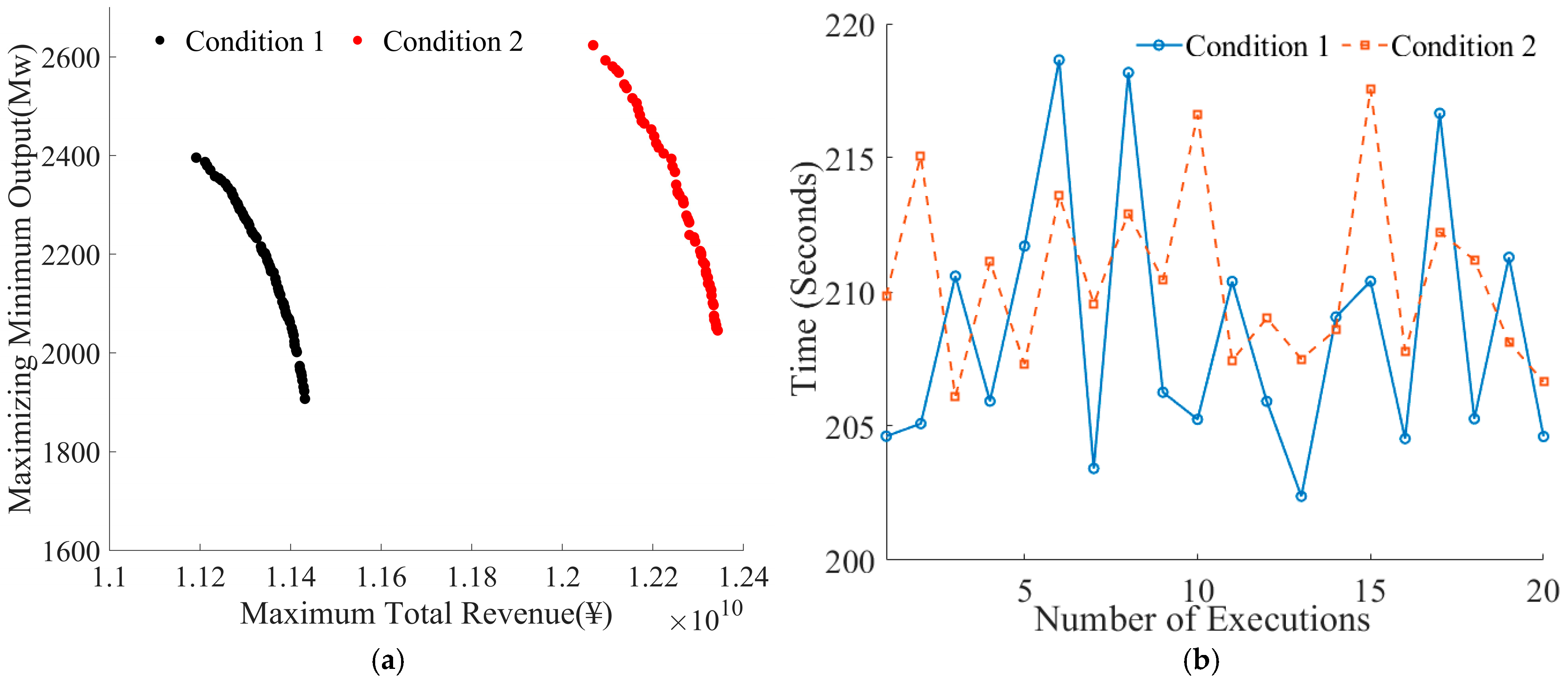
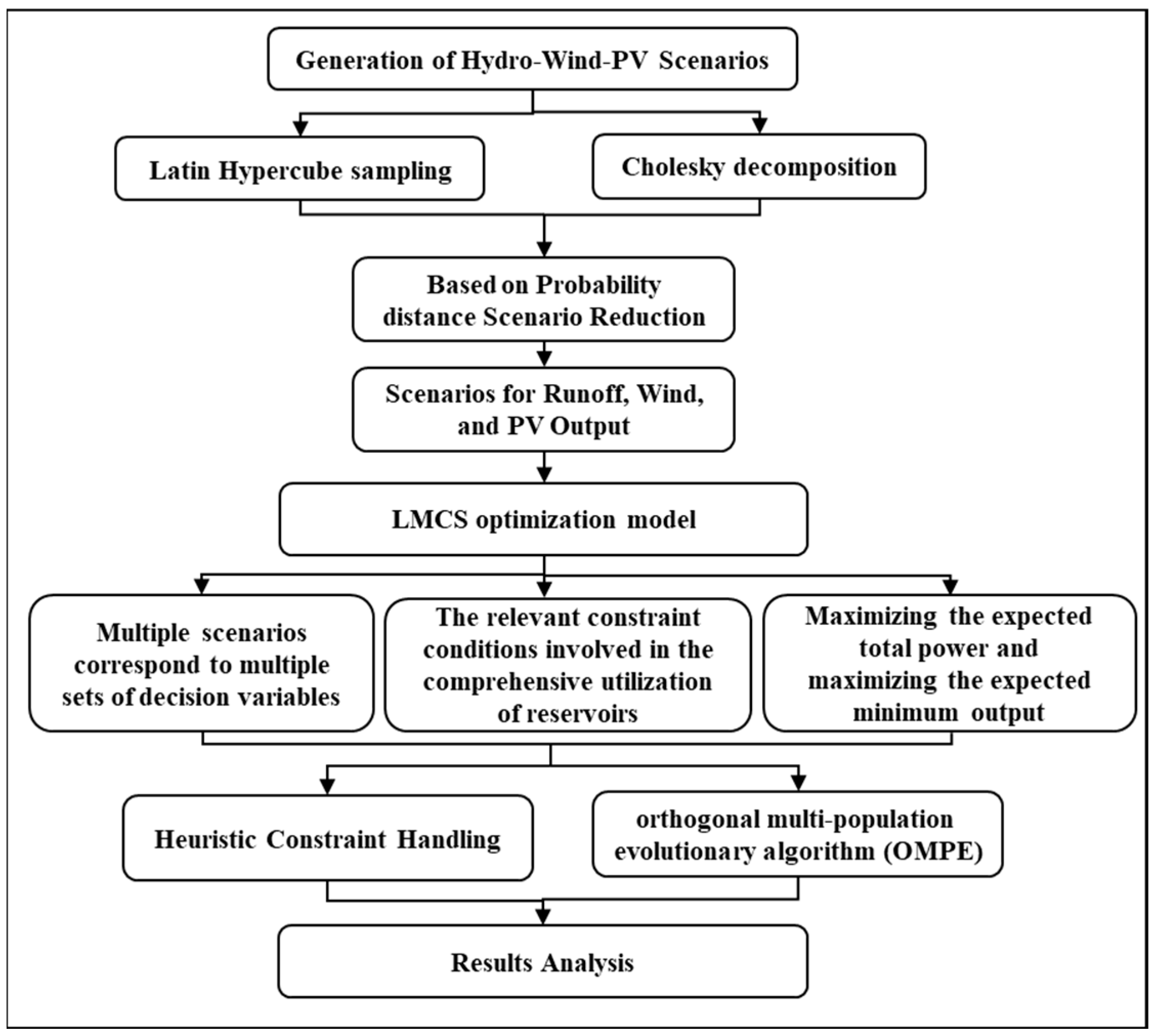
We validate the effectiveness of the algorithm using actual data. Additionally, we perform sensitivity analysis to examine the impact of different numbers of scenarios and water-level restrictions on the scheduling results. This analysis provides key management insights. Figure 1 illustrates the overall framework of the proposed methodology. While the present study focuses on hydro–wind–PV complementarity, the proposed framework could be extended to other multi-energy contexts, such as hydrogen-integrated systems [36] or high-temperature fuel cell hybrid systems [37], where similar stochastic optimization and constraint-handling challenges arise.

2. Generation of Hydro–Wind–PV Scenarios

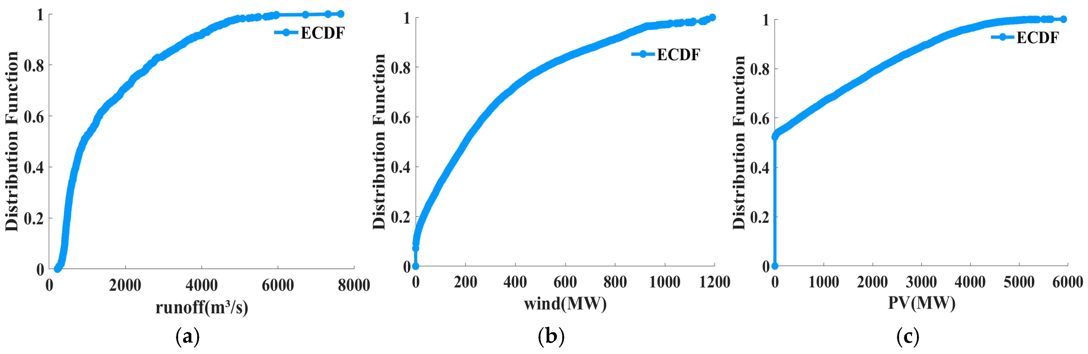
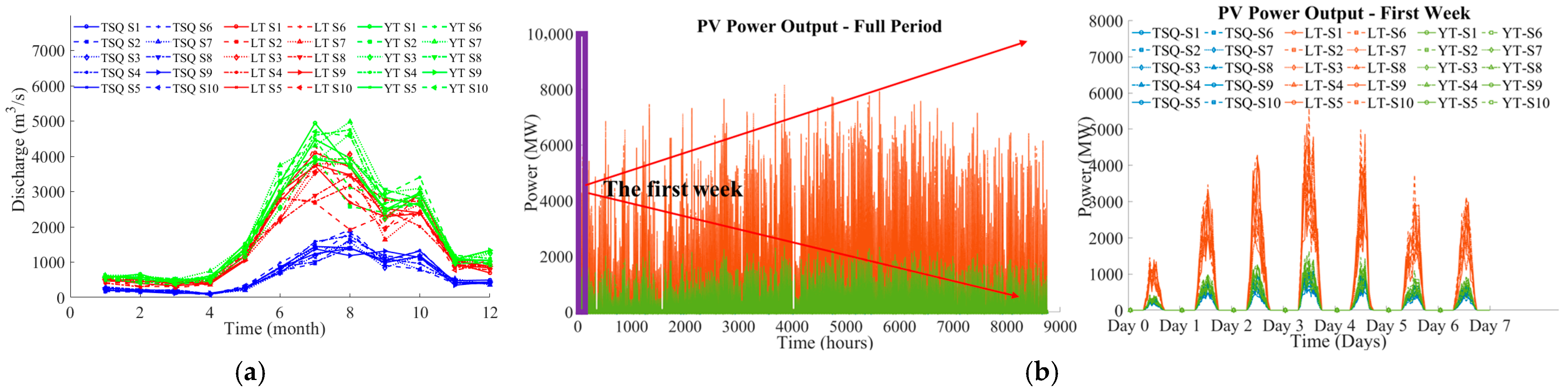
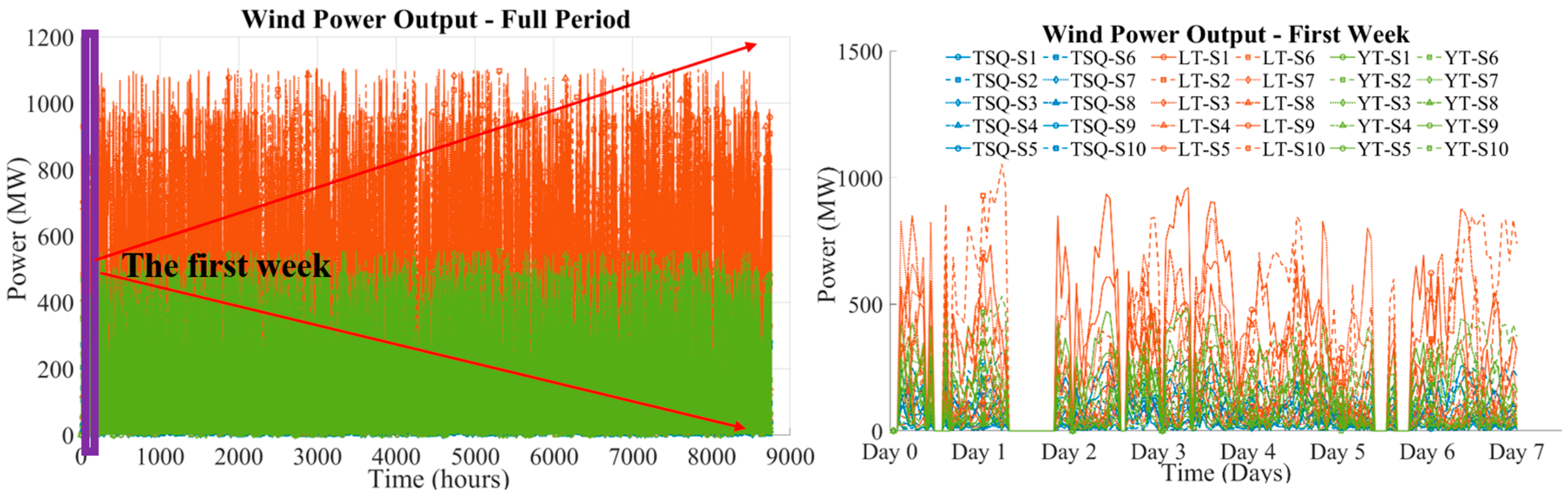
This research leverages archival records of water flow, wind power generation, and solar photovoltaic output to derive their empirical cumulative distribution patterns. The generation of scenarios for these three energy sources is accomplished by integrating Latin hypercube sampling with Cholesky decomposition techniques [13,14]. The overall procedure consists of three steps: (1) generate independent samples using Latin hypercube sampling (LHS); (2) transform the samples to Gaussian space through quantile mapping, which enables the application of Cholesky decomposition; and (3) impose the target correlation structure using Cholesky decomposition. Then, perform an inverse transformation to return the samples to the original space. Cholesky decomposition methods conventionally assume Gaussian-distributed data. Directly applying them to empirical probability distributions from historical records would fail to capture nonlinear interdependencies. To address this challenge, the present work employs quantile mapping to transform historical observations into a standardized normal framework. Within this transformed space, correlation matrices are computed and factorized using triangular matrix factorization. This yields interdependent Gaussian variates. These correlated variables are then transformed back to a uniform probability space. Finally, scenario ensembles are constructed using inverse empirical cumulative distribution functions. Recognizing that computational complexity in scenario-based optimization scales primarily with scenario cardinality, this investigation implements a probabilistic distance-metric approach for scenario pruning, thereby condensing the scenario portfolio to a tractable computational magnitude [15].

2.1. Latin Hypercube Sampling

Latin hypercube sampling (LHS) is an efficient Monte Carlo simulation method that reflects the overall distribution of random variables, avoids duplicate sampling values, and allows the tails of the distribution to participate in sampling. Let $X_1,X_2,\cdots ,X_K$ be K-independent input random variables and $X_K$ be any one of them. The cumulative probability distribution function is shown in Formula (1):

$$Y_k=F_k\left(X_k\right),$$

(1)

In Equation (1), the cumulative probability distribution function is the empirical distribution function calculated from historical data. The basic principle of LHS is as follows: let $N$ be the sampling scale. When sampling each independent random variable, divide the interval [0, 1] of the cumulative probability function $Y_k=F_k\left(X_k\right)$ into $N$ non-overlapping, equidistant subintervals, each with a width of $1/N$. Then, randomly select a sample value $U_n$ of $Y_k$ from each interval.

$$U_n={\displaystyle \frac{U}{N}}+{\displaystyle \frac{n-1}{N}},$$

(2)

In Equation (2), $n$ is a random number in $1,\dots ,N,$ represented as a random interval; $U$ is a random number in the interval of [0, 1]; and $U_n$ is a random number within the $n$th interval.

When sampling occurs within an interval, only one random number $U_n$ is generated, and the interval is excluded from further sampling. Equation (3) can be obtained from Equation (2) as follows,

$${\displaystyle \frac{n-1}{N}}<U_n<{\displaystyle \frac{n}{N}},$$

(3)

In Equation (3), ${\displaystyle \frac{n-1}{N}}$ and ${\displaystyle \frac{n}{N}}$ are the lower and upper bounds of the $n$th interval, respectively.

After obtaining the random number $U_n$ for each interval, apply the inverse transformation of $Y_k=F_k\left(X_k\right)$ to calculate the sampling value $x_{kn}$ of the random variable $X_k$ as shown in Equation (4).

$$x_{kn}=F_k^{-1}\left(U_n\right),$$

(4)

In Equation (4), $F_k^{-1}(\cdot )$ is the inverse transformation of $F_k(\cdot )$. The inverse cumulative distribution function can be obtained by the empirical distribution function.

After collecting $N$ samples of the input random variable $X_k$, they are arranged as a row of the sampling matrix. Once all $K$ random variables are sampled, a $K \times N$ sampling matrix $X_s$ is formed.

2.2. Cholesky Decomposition

Perform quantile transformation on the sampled value $x_{kn}$ to obtain the standard normal variable $z_{kn}$, forming a new sampling matrix $X_s^{\prime }$. Assuming a first-order autoregressive time correlation, calculate the autocorrelation matrix ${\rho }_L$ of historical data in normal space. By applying Cholesky decomposition, a real-valued nonsingular lower triangular matrix $D$ is obtained, as expressed in Equation (5).

$${\rho }_L=D{D}^T,$$

(5)

Generate an independent normal random number matrix $L$ of size $K \times N$. Each row of L represents the positions of elements in the corresponding row of $X_s^{\prime }$. Each row consists of randomly arranged integers from 1 to $N$. By introducing correlation using the Cholesky matrix $D$, a $K \times N$ matrix $G$ is obtained, as shown in Equation (6).

$$G=D^{-1}L,$$

(6)

The correlation coefficient matrix of matrix $G$ is a $K \times K$ identity matrix, indicating no correlation between its rows. If the row elements of the matrix $L$ are rearranged according to the magnitudes of the corresponding elements in $G$, and the rows in $X_s^{\prime }$ are replaced accordingly, the correlation between rows in $X_s^{\prime }$ is reduced. Finally, perform the inverse transformation on $z_{kn}^{\prime }$ in $X_s^{\prime }$, and use the inverse empirical CDF to transform it back to the original distribution space to obtain the final scenario set.

2.3. Scenario Reduction

The computational load of scenario-based planning problems largely depends on the number of scenarios. With too many scenarios, the result has high precision but requires significant computational effort and time. Conversely, too few scenarios cannot guarantee that the optimization results reflect the true randomness of the stochastic variables, leading to low precision in the simulated results. This paper employs scenario-reduction techniques based on a probability metric [33] to decrease the number of scenarios.

For each scenario, specify a probability $p_s$ (where $s=1,2,\dots ,N$), such that $p_s\ge 0$ and the condition ${\sum }_{s=1}^N{p}_s=1$ holds. Let the probability for each scenario be specified as $p_s=1/N$. Let ${\xi }_s$ (for $s=1,2,\dots ,N$) represent the scenario in the sample matrix $X_s$, and $D{T}_{s,s^{\prime }}$ denote the distance between scenario $s$ and ${\mathrm{s}}^{\prime }$, which is the vector norm between scenario $s$ and ${\mathrm{s}}^{\prime }$. The set $s$ represents the initial scenarios, and the set $DS$ represents the scenarios that need to be reduced. The basic steps for scenario reduction are as follows:

Step 1: Set $DS$ as empty and determine the inter-scenario distance metrics as $D{T}_{s,s^{\prime }}=DT({\xi }_s,{\xi }_{s^{\prime }})$.

Step 2: For each scenario $k$, find the scenario $r$ with the shortest distance to scenario $k$, $D{T}_k\left(r\right)=minD{T}_{k,s}$ for all $k\in S,s\in S,k\ne s$.

Step 3: Calculate $P{D}_k\left(r\right)=p_k\ast D{T}_k\left(r\right)$ for all $k\in S$ and identify the scenario index $d$ such that $P{D}_d=minP{D}_k$ for all $k\in S$.

Step 4: Update the set $S=S-\left\{d\right\}$ and $DS=DS+\left\{d\right\}$, and adjust the probability $p_r=p_r+p_d$.

Step 5: Repeat Steps 2–4 until the number of remaining scenarios meets the required criteria.

In Step 4, the equation $p_r=p_r+p_d$ ensures that the sum of the probabilities of the remaining scenarios equals the probability summation across all scenarios before any are eliminated, with the eliminated scenario’s probability assigned a value of zero.

3. Mathematical Model for the LMCS Problem

In this study, we aim to maximize the anticipated total revenue while considering the carbon emission cost spanning the long-term scheduling phase and to maximize the expected minimum output of the multi-energy complementary system in each period. Through the integration of hydrological flow scenarios, wind energy variability, and photovoltaic generation profiles, combined with applicable hydraulic operational constraints, a dual-objective optimization framework is formulated to address the long-term multi-energy complementary scheduling challenge. The mathematical symbols and parameters employed in this framework are delineated in

Table 1. Mathematical model notation.

Index and Sets
$j\in J$	Set of scenarios
$t\in T$	Set of medium- and long-term scheduling periods
$n\in N$	Set of hydropower stations.
$W_n$	Sets of wind power plants at station n
$B_n$	Sets of PV power plants at station n
Parameters
$v$	Hydropower price (¥/MWh)
$v^{wind}$	Wind power price (¥/MWh)
$v^{solar}$	Photovoltaic power price (¥/MWh)
$e_n$	$\mathrm{Life-cycle} \mathrm{emission} \mathrm{factor} \mathrm{of} \mathrm{hydropower} \mathrm{station} n$(tCO2/MWh)
$e_n^{wind}$	$\mathrm{Life-cycle} \mathrm{emission} \mathrm{factor} \mathrm{of} \mathrm{wind} \mathrm{power} \mathrm{station} n$(tCO2/MWh)
$e_n^{solar}$	$\mathrm{Life-cycle} \mathrm{emission} \mathrm{factor} \mathrm{of} \mathrm{photovoltaic} \mathrm{power} \mathrm{station} n$(tCO2/MWh)
$CP$	Carbon price (tCO2/¥)
$E^{LCA}$	Expected total carbon emissions throughout the entire life cycle of the system (tCO2)
$p_j$	$\mathrm{probability} \mathrm{of} \mathrm{each} \mathrm{scenario} j$
$P_{n,j,t}$	$\mathrm{Power} \mathrm{output} \mathrm{at} \mathrm{hydropower} \mathrm{station} n$ $\mathrm{in} \mathrm{the} \mathrm{runoff} \mathrm{scenario} j$ $\mathrm{during} \mathrm{period} t$(MW)
$P_{j,t}^{wind}$	$\mathrm{Wind} \mathrm{power} \mathrm{output} \mathrm{at} \mathrm{scenario} j$ in period (MW)
$P_{j,t}^{solar}$	$\mathrm{PV} \mathrm{power} \mathrm{output} \mathrm{at} \mathrm{scenario} j$ $\mathrm{in} \mathrm{period} t$(MW)
$P_t^{min}$	$\mathrm{Expected} \mathrm{minimum} \mathrm{total} \mathrm{output} \mathrm{of} \mathrm{the} \mathrm{system} \mathrm{in} \mathrm{time} \mathrm{period} t$
$V_{n,j,t}$	$\mathrm{Reservoir} \mathrm{storage} \mathrm{at} \mathrm{hydropower} \mathrm{station} n$ $\mathrm{in} \mathrm{time} \mathrm{periods} t$
$I_{n,j,t}$	Inflow discharge at station n at time t under runoff scenario j
$Q{P}_{n,j,t}$	$\mathrm{Power-generating} \mathrm{flow} \mathrm{at} \mathrm{station} n$ $\mathrm{in} \mathrm{time} t$ $\mathrm{under} \mathrm{runoff} \mathrm{scenario} j$
$S_{n,j,t}$	$\mathrm{Spillage} \mathrm{flow} \mathrm{at} \mathrm{station} n$$\mathrm{in} \mathrm{time} t$$\mathrm{under} \mathrm{runoff} \mathrm{scenario} j$
$\underset{\_}{Q{T}_{n,t}}$, $\overline{Q{T}_{n,t}}$	$\mathrm{Outflow} \mathrm{lower} \mathrm{and} \mathrm{upper} \mathrm{bounds} \mathrm{at} \mathrm{station} n$ $\mathrm{in} \mathrm{time} t$
$\underset{\_}{Q{P}_{n,t}}$, $\overline{Q{P}_{n,t}}$	$\mathrm{Power-generating} \mathrm{flow} \mathrm{lower} \mathrm{and} \mathrm{upper} \mathrm{bounds} \mathrm{at} \mathrm{station} n$ $\mathrm{in} \mathrm{time} t$
$\underset{\_}{P_{n,t}}$, $\overline{P_{n,t}}$	$\mathrm{Power} \mathrm{output} \mathrm{lower} \mathrm{and} \mathrm{upper} \mathrm{bounds} \mathrm{at} \mathrm{station} n$ $\mathrm{in} \mathrm{time} t$
$\underset{\_}{V_{n,t}}$, $\overline{V_{n,t}}$	$\mathrm{Reservoir} \mathrm{storage} \mathrm{lower} \mathrm{and} \mathrm{upper} \mathrm{bounds} \mathrm{at} \mathrm{station} n$ $\mathrm{in} \mathrm{time} t$
$Z_{n,Ini}$	$\mathrm{Initial} \mathrm{water} \mathrm{levels} \mathrm{at} \mathrm{station} n$
$Z_{n,End}$	$\mathrm{Final} \mathrm{water} \mathrm{levels} \mathrm{at} \mathrm{station} n$
$f_n^{zy}\left(·\right)$	Nonlinear function between water level and reservoir storage
$f_n^{down}\left(·\right)$	Nonlinear function between tailwater level and outflow discharge at station n
$Z_{n,j,t}$	Water level at station n in time t under the j runoff scenario
$Z_{n,j,t}^d$	Tailwater level at station n in time t under the j runoff scenario
$H_{n,j,t}$	$\mathrm{Hydraulic} \mathrm{head} \mathrm{at} \mathrm{station} \mathrm{n} \mathrm{in} \mathrm{time} \mathrm{t} \mathrm{under} \mathrm{runoff} \mathrm{scenario} j$
$K_n$	$\mathrm{Power} \mathrm{generation} \mathrm{coefficient} \mathrm{at} \mathrm{station} n$
$F_n$	Outputs of hydro power plants
$F_i$	Outputs of wind power plants
$F_j$	Outputs of PV power plants
$\Delta T$	Length of the long-term scheduling period
$\Omega \left(n\right)$	$\mathrm{Upstream} \mathrm{reservoirs} \mathrm{of} \mathrm{reservoir} n$
$T{C}_n^{max}$	$\mathrm{Maximum} \mathrm{integrated} \mathrm{hydro}–\mathrm{wind}–\mathrm{PV} \mathrm{transmission} \mathrm{capacity} \mathrm{at} \mathrm{station} n$.
Decision Variables
$Q{T}_{n,j,t}$	$\mathrm{The} \mathrm{outflow} \mathrm{discharge} \mathrm{of} \mathrm{hydropower} \mathrm{station} n$ $\mathrm{during} \mathrm{time} \mathrm{period} t$ $\mathrm{under} \mathrm{the} j$ runoff scenario

.

The mathematical model for the LMCS problem can be formulated as follows:

(1)

Objective functions

$$\begin{gathered} Max F=\left({\sum }_{n\in N}{\sum }_{j\in J}{\sum }_{t\in T}(v{P}_{n,j,t}+v^{wind}{P}_{j,t}^{wind}+v^{solar}{P}_{j,t}^{solar}){.p}_j\right)\Delta T-CP\cdot E^{LCA}, \\ {E}^{LCA}=\left({\sum }_{n\in N}{\sum }_{j\in J}{\sum }_{t\in T}(e_n{P}_{n,j,t}+e_n^{wind}{P}_{j,t}^{wind}+e_n^{solar}{P}_{j,t}^{solar}){.p}_j\right)\Delta T, \end{gathered}$$

(7)

$$Max P_t^{min}=\underset{t\in T}{\mathit{min}}{\sum }_{n\in N}{\sum }_{j\in J}(P_{n,j,t}+P_{j,t}^{wind}+P_{j,t}^{solar}{).p}_j,$$

(8)

(2)

Constraints

$$V_{n,j,t+1}=V_{n,j,t}+I_{n,j,t}+{\sum }_{m\in \Omega \left(n\right)}Q{T}_{m,j,t}-Q{T}_{n,j,t},\forall n\in N,t\in T,j\in J,$$

(9)

$$Q{T}_{n,j,t}=Q{P}_{n,j,t}+S_{n,j,t},\forall n\in N,t\in T,j\in J,$$

(10)

$$\underset{\_}{Q{T}_{n,t}}\le Q{T}_{n,j,t}\le \overline{Q{T}_{n,t}},\forall n\in N,t\in T,j\in J,$$

(11)

$$\underset{\_}{Q{P}_{n,t}}\le Q{P}_{n,j,t}\le \overline{Q{P}_{n,t}},\forall n\in N,t\in T,j\in J,$$

(12)

$$\underset{\_}{P_{n,t}}\le P_{n,j,t}\le \overline{P_{n,t}},\forall n\in N,t\in T,j\in J,$$

(13)

$$\underset{\_}{V_{n,t}}\le V_{n,j,t}\le \overline{V_{n,t}},\forall n\in N,t\in T,j\in J,$$

(14)

$$Z_{n,j,1}=Z_{n,Ini},\forall n\in N,j\in J,$$

(15)

$$Z_{n,j,T}=Z_{n,End},\forall n\in N,j\in J,$$

(16)

$$V_{n,j,t}=f_n^{zy}\left(Z_{n,j,t}\right),\forall n\in N,t\in T,j\in J,$$

(17)

$$Z_{n,j,t}^d=f_n^{down}\left(Q{T}_{n,j,t}\right),\forall n\in N,t\in T,j\in J,$$

(18)

$$H_{n,j,t}={\displaystyle \frac{Z_{n,j,t+1}+Z_{n,j,t}}{2}}-Z_{n,j,t}^d,\forall n\in N,t\in T,j\in J,$$

(19)

$$P_{n,j,t}=K_n.H_{n,j,t}.Q{P}_{n,j,t},\forall n\in N,t\in T,j\in J,$$

(20)

$${\sum }_{i\in W_n}{F}_i+{\sum }_{j\in B_n}{F}_j+F_n\le T{C}_n^{max},\forall i\in W_n,j\in B_n,n\in N,$$

(21)

The objective expressed in Equation (7) aims to maximize the expected total revenue of the hydro–wind–PV complementary system, while Equation (8) seeks to maximize the expected minimum power output. The carbon emission term in the objective function is determined using life-cycle average emission coefficients and market-based carbon prices. Specifically, $e_n$, $e_n^{wind}$, and $e_n^{solar}$ represent the full life-cycle emission coefficients for each power generation technology. These values are derived from Zhang et al. [38] and reflect embedded life-cycle averages rather than marginal operational emissions.

The carbon price $CP$ is obtained from the regional carbon trading market and represents the current economic cost of emitting one ton of CO₂. Incorporating carbon prices into the objective function effectively incentivizes low-carbon operational strategies. By combining life-cycle emission factors with market-based carbon pricing, our model internalizes the environmental externalities of power generation within long-term planning. This approach is consistent with both the physical reality of full-cycle emissions and the economic mechanisms of the carbon market.

Equations (9) and (10) represent the water balance constraints. Equations (11) and (12) impose limitations on the outflow discharge. Equation (13) defines the constraints on power generation output. Equation (14) specifies the reservoir storage limits. Equations (15) and (16) describe the initial and terminal water level conditions. Equation (17) characterizes the relationship between water level and storage. Equation (18) represents the relationship between tailwater level and outflow. Equations (19) and (20) correspond to the hydropower generation function. Finally, Equation (21) restricts the transmission capacity.

4. Solution Method for the LMCS Problem

4.1. Framework of the OMPE Algorithm

The LMCS model exhibits pronounced nonlinear characteristics derived from its hydroelectric generation functions and multiple nonlinear constraints. Considering the inherent NP-hard nature of dynamic economic dispatch (DED) problems, the integration of uncertainty factors substantially exacerbates the computational complexity of obtaining optimal solutions for LMCS systems. To address the efficiency-accuracy trade-off within computationally feasible budgets, an orthogonal multi-population evolutionary (OMPE) algorithm is developed through the innovative integration of orthogonal experimental design with collaborative multi-population optimization mechanisms. This proposed methodology extends the multi-population evolutionary framework originally established for multi-objective optimization benchmarks in [39], with enhanced optimization mechanisms specifically engineered to improve solution efficiency for complex system problems. Unlike traditional evolutionary algorithms that use a single population and Pareto dominance, the OMPE algorithm introduces an additional elite population. This population is updated according to $\epsilon$-Box dominance rules. Concurrently, a hybridization of diverse recombination mechanisms is incorporated to enhance the algorithm’s adaptability across heterogeneous problem landscapes. This architectural feature ensures operational resilience. It achieves this through dynamic operator selection, which is governed by environmental feedback signals. Particularly, this study proposes an orthogonal population initialization algorithm to enhance spatial uniformity and solution diversity preservation in high-dimensional search spaces. The population is first initialized according to the population encoding rules through symmetric discretization of continuous variables and orthogonal array construction. This ensures systematic coverage of feasible regions while eliminating solution clustering biases inherent in random sampling methods. 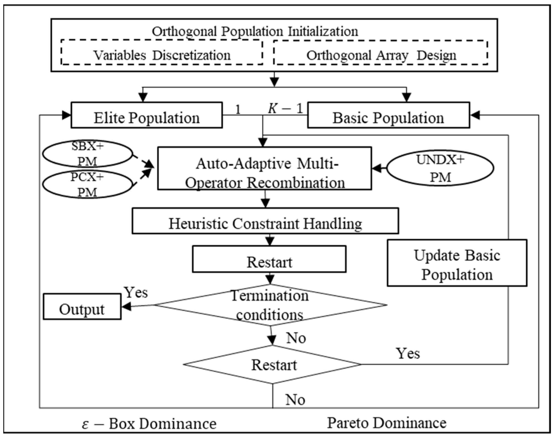Then, based on the orthogonal initial solutions, the population is divided into basic and elite populations according to the $\epsilon$-Box dominance rule. The OMPE framework builds a flexible pool of recombination operators, and the most promising operator is adaptively chosen based on its performance on the specific problem at hand. A well-tailored constraint-handling strategy is developed to repair the new populations to feasibility. In addition, a restart mechanism is also integrated in the algorithm, where the elite population is reshuffled if the solution cannot be improved during a predetermined number of iterations. The pseudocode for the solution method of LMCS is shown in Figure 2, and the following provides a detailed explanation of the key solution ideas.

4.2. Orthogonal Population Initialization

The proposed orthogonal population initialization algorithm is described as follows.

For the general optimization problem, where $X=\left(x_1,x_2,\dots ,x_N\right)\in \Omega$, $\mathrm{f}$ is the objective function, $\Omega =\left\{\left(x_1,x_2,\dots ,x_N\right)\right|l_i\le x_i\le u_i,i=1,2,\dots ,N\}$. The orthogonal population encoding framework provides a structured approach for initializing populations in evolutionary algorithms. By applying principles of orthogonal design, it improves the diversity of candidate solutions and enhances their distribution across the search space. The framework is systematically structured through two pivotal steps to ensure optimal exploration of the solution space.

Step 1: Discretization of Continuous Variables:

For each continuous decision variable $x_i\in [l_i,u_i]$, a symmetric quantization scheme with $Q_1$ discrete levels ($Q_1$: odd integer) [38] is applied to ensure uniform domain partitioning:

$$r_i^j=\left\{\begin{array}{c}{l}_i j=1\\ l_i+\left(j-1\right) {\displaystyle \frac{{(u}_i-l_i)}{Q_1-1}} 2\le j\le Q_1-1\\ u_i j=Q_1 \end{array}\right.,$$

(22)

This discretization preserves boundary integrity while establishing equidistant sampling intervals, critical for maintaining solution space representativeness.

Step 2: Orthogonal Array Design:

An orthogonal array $L_{M_1}\left(Q_1^{N_1}\right)$ is constructed under constrained optimization criteria:

$$\left\{\begin{array}{c}\mathrm{M}\mathrm{i}\mathrm{n}\mathrm{i}\mathrm{m}\mathrm{i}\mathrm{z}\mathrm{e}:M_1=Q_1^J,\\ N_1={\displaystyle \frac{Q_1^J-1}{Q_1-1}}\ge N,\\ M_1\ge NP,\end{array}\right.$$

(23)

where $M_1$ denotes the number of experiments (candidate solutions), $N_1$ represents the dimensionality, and $NP$ is the predefined population size. The orthogonal array, generated via algorithms ensuring uniform dispersion and pairwise independence (e.g., the method in [38]), establishes a structured sampling framework. For instance, $L_9\left(3^4\right)$ defines nine experiments with four variables, each containing three levels.

The orthogonal array is mapped to a candidate population (orthogonal population, OP) by encoding each row as an individual $X_i$. For hydropower scheduling applications, $X$ is formulated as $X=\left\{{QT}_{111},\dots ,{QT}_{11T},{QT}_{121},\dots ,{QT}_{12T},\dots ,{QT}_{1JT},\dots ,{QT}_{NJT}\right\},$ where ${QT}_{njt}$ defines the discharge of the $n$th reservoir at period $t$ under scenario $j$ and $Q{T}_{n,j,t}\in \left[\underset{\_}{Q{T}_{n,t},}\overline{Q{T}_{n,t}}\right]$.

4.3. $\mathit{\epsilon }$-Box Dominance Rule

The $\epsilon$-Box dominance is based on $\epsilon$-dominance: for a given $\epsilon >0$, vector $u=\left(u_1,u_2,\dots ,u_M\right)$ $\epsilon$-dominates another vector $v=\left(v_1,v_2,\dots ,v_M\right)$ if and only if for all $\forall i\in \left\{1,2,\dots ,M\right\},u_i\le v_i+\epsilon$ and there exists at least one $j\in \left\{1,2,\dots ,M\right\}$, such that $u_j<v_i+\epsilon$. When the obtained solutions cause the objective function values to cross the $\epsilon$ range, $\epsilon$-dominance directly determines the dominance relationship between populations. 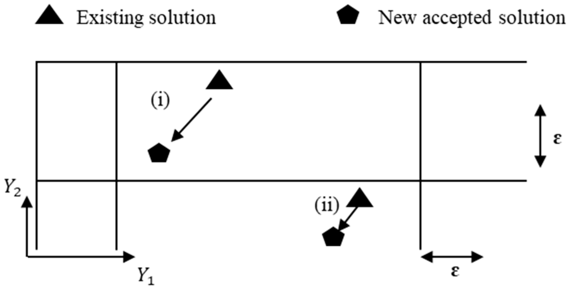When the solutions obtained from different populations fall within the range defined by $\epsilon$, forming a “box-like” region, the population that is closest to the optimal target is then selected based on its proximity to the best objective value. In the case of the two objective functions in LMCS being maximization problems, the solution that is closer to the upper-right corner of the “box” will dominate other populations. As intuitively illustrated in Figure 3, the threshold $\epsilon$ effectively governs the optimization direction. In case (i), the new solution significantly exceeds the $\epsilon$ threshold range in both $Y_1$ and $Y_2$ objectives, forming a clear advantage over the Pareto front. In contrast, case (ii) shows that although the new solution achieves a slight improvement in partial objectives, it fails to breach the $\epsilon$-defined neighborhood boundary and thus is unable to activate the $\epsilon$-Box rule effectively.

The Pareto rule will be used in the basic population. Pareto dominance is a fundamental concept in multi-objective optimization used to compare solutions based on their performance across multiple conflicting objectives. A solution $x$ is said to Pareto-dominate another solution $y$ if $x$ is no worse than $y$ in all objectives and strictly better in at least one. Solutions that are not dominated by any other are considered Pareto optimal, forming the Pareto front.

4.4. Multiple Recombination Operators

The OMPE framework adopts a multi-operator fusion mechanism, discarding the traditional approach of using a single genetic recombination operator. Operators that perform well during the iterative process are assigned higher selection weights, while each recombination operator is initially assigned an equal selection weight (e.g., 1/total number of operators). An adaptive feedback architecture is implemented to quantitatively assess operator efficacy, with selection weights dynamically adjusted across evolutionary cycles. This mechanism employs ε-Box dominance analysis within non-dominated solution sets as the performance metric, whereby operator productivity is quantified by its contribution to elite solution generation. Operators demonstrating superior Pareto-frontier expansion capabilities receive proportionally enhanced selection probabilities, thereby establishing self-adaptive evolutionary pressure through solution-space coverage evaluation. The recombination operators employed in the algorithm consist of three recombination mechanisms—Simulated Binary Crossover (SBX), Parent-Centric Crossover (PCX), and Unimodal Normal Distribution Crossover (UNDX)—along with the Polynomial Mutation (PM) operator [33].

4.5. Heuristic Method for Managing Constraints

The operational model features a coupled constraint architecture, which leads to cascading parameter adjustments. As a result, systematic constraint coordination is required. Predefined boundary conditions, such as initial and final reservoir elevations, and cumulative discharge quantities become deterministic variables. These can be calculated using hydraulic conservation principles. This study adopts a heuristic repair strategy based on adjacent time periods. It first ensures that the water balance constraint is satisfied for each time interval. Then, it corrects the reservoir storage by adjusting water release without violating the water balance [40].

4.5.1. Handling Dynamic Water Balance Constraint

First, calculate the amount of water exceeding the reservoir capacity constraint. Then, adjust the outflow discharge for the corresponding period based on the violation amount, ensuring that the reservoir storage returns to within the constraint range. The procedure balances the total water volume over the entire scheduling horizon and distributes any remaining imbalance locally to adjacent periods. The detailed steps for managing the dynamic water balance constraint for reservoir $n$ are as follows:

Step 1: Calculate the difference between the water usage and the constrained water volume for reservoir $n$ over the entire scheduling period using Equations (6) and (7), denoted as $\Delta {QT}_{n,j,t}$. This global imbalance represents the total volume that must be redistributed across all time periods.

Step 2: Distribute the water volume difference across all periods, adjusting the flow using the following formula:

$${QT}_{n,j,t}={QT}_{n,j,t}+{\displaystyle \frac{\Delta {QT}_{n,j,t}}{\Delta T}},$$

(24)

Apply the flow range constraint to the adjusted flow ${QT}_{n,j,t}$:

$${QT}_{n,j,t}=\left\{\begin{array}{c}\underset{\_}{Q{T}_{n,t}}, if {QT}_{n,j,t}<\underset{\_}{Q{T}_{n,t}}\\ {QT}_{n,j,t}, if \underset{\_}{Q{T}_{n,t}}<{QT}_{n,j,t}<\overline{Q{T}_{n,t}}\\ \overline{Q{T}_{n,t}}, if {QT}_{n,j,t}>\overline{Q{T}_{n,t}}\end{array}\right.,$$

(25)

Step 3: Recalculate the volume difference. If $\Delta {QT}_{n,j,t}=0$, go to Step 7; otherwise, go to Step 4.

Step 4: Set a counter $n=1$.

Step 5: Randomly and non-repetitively select a scheduling time period, $t$, and adjust the outflow discharge for that period to satisfy the dynamic water balance constraint as follows:

$${QT}_{n,j,t}={QT}_{n,j,t}+\Delta {QT}_{n,j,t},$$

(26)

The above flow range constraint conditions can also be applied for adjustment. This step ensures that the remaining imbalance is redistributed locally to specific periods, rather than uniformly across all periods.

Step 6: If $n\le \Delta T$, let $n=n+1$ and return to Step 5; otherwise, proceed to Step 7.

Step 7: The process for handling the dynamic water balance constraint is complete.

4.5.2. Handling Reservoir Storage Regulation

For the reservoir storage constraint, the proposed strategy involves first calculating the excess water volume that exceeds the storage limit and then adjusting the outflow discharge for the corresponding time period based on the extent of the violation. This adjustment brings the reservoir storage back within the allowable limits. To maintain dynamic water balance, the strategy also makes a compensatory adjustment to the flow in the subsequent period. This ensures that the current storage meets the constraint without affecting the storage in other periods. If the adjustment reaches the outflow bounds and the violation persists, the remaining excess or deficit is propagated to the next reservoir in the cascade. The specific steps are described as follows:

Step 1: First, calculate the reservoir storage $V_{n,j,t}$ for each time period.

Step 2: Check whether the reservoir storage meets the required range. If it does not meet the requirement, determine whether it exceeds the maximum storage limit. If it exceeds, calculate the excess volume $\Delta V_{n,j,t}=(V_{n,j,t}-\overline{V_{n,t}})/\Delta t$ and distribute it evenly across the adjustment periods in the planning horizon to perform Step 3. If it is below the minimum limit, calculate the shortfall $\Delta V_{n,j,t}=(\underset{\_}{V_{n,t}}-V_{n,j,t})/\Delta t$ and distribute it evenly across the adjustment periods to perform Step 4.

Step 3: Transfer the excess volume to the outflow discharge of adjacent reservoirs while adhering to outflow discharge constraints. If the outflow exceeds the maximum allowable limit, calculate $\Delta V_1=\Delta V_{n,j,t}-(V_{n,j,t}-\overline{V_{n,t}})$ and continue to distribute it across the outflow discharges of adjacent reservoirs until the maximum acceptable outflow discharge level is reached. If the outflow is below the minimum allowable level, calculate $\Delta V_1=\Delta V_{n,j,t}-(\underset{\_}{V_{n,t}}-V_{n,j,t})$ and adjust the outflow discharge of adjacent reservoirs to ensure it meets the minimum discharge level. If the adjustment reaches the flow bounds and the excess water still remains, the remaining excess is propagated to the downstream reservoir through the cascade connection.

Step 4: Similarly, transfer the shortfall to the outflow discharge of adjacent reservoirs while adhering to outflow discharge constraints. If the discharge still exceeds the allowable maximum, continue to distribute it to adjacent reservoirs until the maximum acceptable outflow level is reached. If the discharge is below the minimum allowable level, adjust the outflow of adjacent reservoirs to ensure it meets the minimum discharge level. If the shortfall cannot be fully compensated within the current reservoir due to flow bounds, the remaining deficit is propagated upstream, effectively retaining more water in the upstream reservoir.

Step 5: Iterate the adjustments until the reservoir storage levels in all planning periods fall within the specified range.

5. Results and Discussion

5.1. Case Study Introduction

The Hongshui River features multiple cascaded hydropower stations. In this paper, the runoff data from three cascaded hydropower annual-regulation stations—Tianshengqiao I, Longtan, and Yantan—along the Hongshui River Basin are selected for a case study [41], as shown in Figure 4.

Generation data comes from multiplying normalized annual profiles (Hongshui River) by wind/PV installed capacities. The runoff data mentioned above have a monthly time step, while the wind and PV output data have an hourly time step. The runoff data are from 60 years after 1951, and wind and PV energy data were systematically generated based on available data from a certain year. The basic information of the hydropower stations is presented in

Table 2. Operational parameters of the studied power stations.

Name	Basin Area (km2)	Installed Capacity (MW)	Regulating Storage (Billion m3)	Wind Energy Facility Capacity (MW)	PV Energy Facility Capacity (MW)	Hydro Energy Facility Capacity (MW)
Tianshengqiao I	50,139	1200	5.796	360	1640	1200
Longtan	98,500	6300	11.2	1230	7160	6300
Yantan	106,580	1810	0.425	620	2105	1810

. The related price and life-cycle emission factors are taken from [42] and are shown in

Table 3. The related price and life-cycle emission factors.

Name	Value
$v$	320
$v^{wind}$	330
$v^{solar}$	250
$e_n$	0.0188
$e_n^{wind}$	0.0142
$e_n^{solar}$	0.0100
$CP$	72.4

.

The OMPE algorithm is configured with a total population size of 100. This includes a basic population of 70 individuals and an elite population of 30 individuals. The basic population is updated using Pareto dominance, while the elite population follows the $\epsilon -Box$ dominance rule. For the two objective functions, the $\epsilon$ parameters are set to 500 and 5.5, respectively. For orthogonal initialization, the number of discrete levels is set to $Q_1=3$. Four recombination operators are employed: SBX, PCX, UNDX, and PM. Each operator is initially assigned a selection probability of 0.25. These probabilities are adaptively adjusted during evolution based on operator performance. The crossover probability is set to 0.9, and the mutation probability is set to ${\displaystyle \raisebox{1ex}{$1$}\!\left/ \!\raisebox{-1ex}{$D$}\right.}$, where $D$ is the number of decision variables. The distribution indices for SBX and PM are both set to 20. PCX and UNDX adopt the default parameter values commonly used in real-coded evolutionary algorithms. The algorithm terminates when the maximum number of generations reaches 300 or when the elite population shows no improvement for 30 consecutive generations. If the elite population stagnates for 20 consecutive generations, a partial elite restart is triggered to help escape local optima. The algorithm was developed in C with VS 2022 on Win10 (i5-8500 CPU, 8 GB RAM) and run 20 times.

5.2. Experimental Results

5.2.1. Results of Scenario Generation

Based on the temporal interdependence of runoff, wind, and PV resources, this study generates 1000 scenarios through LHS combined with Cholesky decomposition. To capture the probability characteristics of actual runoff and wind and PV power output, the study calculates the empirical distribution function (ECDF) of runoff, wind, and PV power output based on existing time-series data, as shown in Figure 5.

Using the obtained empirical distribution function, initial scenario sets for runoff, wind and PV are generated according to the methods in Section 2.1 and Section 2.2. To satisfy the requirements of subsequent models and algorithms regarding the number of scenarios, the scenario set for each resource is reduced to 10 according to the scenario reduction procedure described in Section 2.3.

This study focuses on the analysis of runoff as well as wind–PV power output from three hydropower stations. The scenario-generation process for runoff and wind–PV output is identical for each station. Figure 6 illustrates the generated scenarios of runoff and wind–PV power output for the Tianshengqiao I Hydropower Station.

The results indicate that the proposed scenario-generation approach effectively captures the variation patterns of different variables within the multi-energy complementary system. The generated runoff and wind–PV scenarios display overall continuity and lack significant random fluctuations. This demonstrates that the proposed method can accurately represent the temporal correlations among hydropower, wind power, and solar power.

To further validate the reasonableness of the generated scenarios, this study adopts the autocorrelation coefficient (ACF) as an indicator of temporal correlation. The ACF reflects the degree of temporal correlation in a variable. As the lag time increases, the autocorrelation coefficient gradually decreases. By analyzing the magnitude and variation of the ACF, the performance of the generated scenarios in capturing temporal characteristics can be assessed. The formula is shown as follows:

$${\rho }_k={\displaystyle \frac{{\sum }_{t=1}^{n-k}(r_t-\overline{r})(r_{t+k}-\overline{r})}{{\sum }_{t=1}^n{(r_t-\overline{r})}^2}},$$

(27)

where $r_t$ represents the value of the $t$-th month and $k$ represents the number of time intervals. Term $\overline{r}$ represents the mean and ${\rho }_k$ represents the autocorrelation coefficient of lagged $k$-order.

This study compares the ACF values of historical runoff, wind power, and PV output with those of the generated scenarios. The results are shown in Figure 7. The ACF of the runoff, wind and PV output scenario set closely follows the trend of autocorrelation coefficient changes in the historical sequence. This supports the observation that the generated scenario set effectively captures the temporal correlation of runoff, wind, and PV power output.

5.2.2. Inter-Algorithm Performance Assessment and Operator Contribution Analysis

Serving as computational inputs for the optimization framework, the hydraulic discharge, wind capacity, and solar generation patterns across ten probabilistic realizations are depicted in Figure 8 and Figure 9. To substantiate the methodological validity of the proposed approach, and acknowledging procedural parallels between NSGA-II’s multi-criteria optimization mechanics and those embedded within OMPE, this investigation conducts comparative benchmarking against NSGA-II for the long-term multi-energy scheduling challenge. To evaluate the contribution of individual components and dominance mechanisms within OMPE, ablation studies are performed by systematically excluding single operators, substituting $\epsilon$-Box dominance with classical Pareto dominance, and replacing orthogonally-designed initialization with stochastic initialization schemes.

To evaluate the performance of the OMPE and the benchmark algorithms, we employ two widely used multi-objective quality indicators: the Coverage-metric and the Space-metric. The Coverage-metric (C-Metric) indicates the dominance ratio metric [39], used to evaluate the quality of the Pareto solution set by computing the dominance ratio among solutions. It is defined as the fraction of solutions in set $X_2$ that are dominated by solution $X_1$:

$$C\left(X_1,X_2\right)={\displaystyle \frac{\left|\left\{x_2\in X_2|\exists x_1\in X_1:x_1 dominate x_2\right\}\right|}{\left|X_2\right|}},$$

(28)

The Space-metric (S-Metric) measures the distribution range of the Pareto solution set in the objective space of a multi-objective optimization problem by determining a reasonable reference point and calculating the area covered by two solution sets, $X_1$ and $X_2$, in the objective space, with the specific calculation method provided in [39]. The hypervolume between a reference point and non-dominated solutions is calculated as follows:

$$S\left(x\right)=Volume\left({\bigcup }_{x\in X}\left[x_1,r_1\right]\times \dots \times \left[x_k,r_k\right]\right),$$

(29)

where $r$ is the reference point. Higher values indicate better convergence and diversity.

Table 4. C-Metric and S-Metric values for OMPE, NSGA-II, and the variants of OMPE.

Combination	$\mathit{B}\mathit{t}$	$\mathit{A}\mathit{g}$	$\mathit{S}\mathit{D}$	Combination	$\mathit{B}\mathit{t}$	$\mathit{A}\mathit{g}$	$\mathit{S}\mathit{D}$
$C(A,B)$	1	0.99	0.01	$C(E,A)$	0	0	0
$C(A,C)$	1	0.97	0.01	$C(F,A)$	0	0	0
$C(A,D)$	1	0.99	0.02	$S\left(A\right)$	1.46 × 109	3.96 × 108	1.42 × 107
$C(A,E)$	1	0.98	0.02	$S\left(B\right)$	9.81 × 108	3.71 × 108	1.21 × 107
$C(A,F)$	1	0.98	0.01	$S\left(C\right)$	9.72 × 108	3.85 × 108	1.10 × 107
$C(B,A)$	0	0	0	$S\left(D\right)$	8.12 × 108	2.63 × 108	2.45 × 107
$C(C,A)$	0	0	0	$S\left(E\right)$	6.71 × 108	2.25 × 108	2.41 × 107
$C(D,A)$	0	0	0	$S\left(F\right)$	6.89 × 108	2.21 × 108	2.05 × 107

summarizes the statistical results of the C-metric and S-metric values over 20 independent runs. For the C-metric, OMPE (denoted as A) achieves a maximum dominance fraction (Bt) of 1.00 and an average dominance proportion (Ag) of 0.99 against NSGA-II (B), indicating that nearly all solutions of NSGA-II are dominated by OMPE. Similarly, OMPE dominates MOEA/D (C) and all OMPE variants (D–F) with average C-metric values above 0.97, while the reverse C-metric values (C(B,A), C(C,A), etc.) are uniformly zero, confirming that OMPE consistently outperforms the compared algorithms across all 20 runs.

For the S-metric (hypervolume), OMPE achieves the highest average value (3.96 × 10⁸) with a low standard deviation (1.42 × 10⁷), demonstrating superior convergence and diversity. To further validate the statistical significance of the performance differences, we conduct the Wilcoxon rank sum test (WRS) on the S-metric values obtained from 20 independent runs. As shown in

Table 5. Results of Wilcoxon rank sum test for S-metric.

Comparison	WRS	p-Value
A vs. B	23	<0.001
A vs. C	87	<0.001
A vs. D	0	<0.001
A vs. E	0	<0.001
A vs. F	0	<0.001

, the results show that OMPE achieves significantly higher hypervolume values than NSGA-II (p < 0.001), MOEA-D (p < 0.001), and all OMPE variants (p < 0.001). These statistical tests confirm that the observed performance advantages of OMPE are not caused by random variations and are statistically significant.

The Pareto fronts obtained under different conditions are compared in Figure 10a. Notably, the Pareto front derived from the OMPE algorithm consistently outperforms NSGA-II, demonstrating its superior performance. Moreover, the comparison results of OMPE and its variants indicate the following: (i) the orthogonal initialization method significantly improves the approximation to the real Pareto-front, (ii) removing each recombination operator undermines the performance of the OMPE algorithm, and (iii) the $\epsilon$-Box rule significantly enhances the performance of the OMPE algorithm. It should be noted that OMPE’s superior performance comes with a slight increase in computational burden, as shown in Figure 10b, where OMPE requires slightly longer but comparable computational time relative to other approaches.

Additionally, regarding economic returns for the Tianshengqiao I, Longtan, and Yantan generation facilities, NSGA-II implementation yielded aggregate revenues of 2310.26 million, 6720.84 million, and 3149.44 million, respectively. Conversely, the framework and OMPE methodology advanced herein generated 2337.27 million, 7322.07 million, and 3224.47 million, respectively, manifesting enhancements of 5.07%, 8.95%, and 2.38%, culminating in an aggregate improvement of 5.46%. Concerning baseload capacity assurance, OMPE achieves 2722.31 MW from the objective formulation, representing a 3.89% elevation over NSGA-II’s 2620.48 MW output. These empirical outcomes validate the computational efficacy of the OMPE algorithmic framework.

5.2.3. Impact of Different Boundary Conditions on the LMCS Problem

This study evaluates the adaptive properties by examining how different initial and final water levels of the reservoirs, which are listed in

Table 6. Boundary conditions of different initial and final water levels.

Name	Condition 1		Condition 2
	Initial	Final	Initial	Final
Tianshengqiao I	773	780	773	750
Longtan	359.3	375	359.3	350
Yantan	219	223	219	219

, affect scheduling results.

Figure 11a presents the Pareto frontier obtained, and Figure 11b shows the variation in the duration of 20 runs under different conditions. It can be observed that the diversity of the non-dominated solutions is rich and uniformly distributed, while there is a conflicting relationship between the two objective functions. Compared with the results obtained in Condition 1, where the reservoirs need to store water during the scheduling period, the objectives in Condition 2 increase significantly due to more abundant water usage. The computational time exhibits minimal fluctuations, highlighting the algorithm’s suitability and stability in solving the problem. The duration of each execution exhibits little volatility, highlighting the suitability and stability of the algorithm for problem-solving.

To begin, the Pareto optimal solution set must first be derived under different scenarios. Subsequently, decisions are made based on the method outlined in [43]. Obviously, each scenario corresponds to a specific scheduling result. To investigate the impacts of different boundary conditions on scheduling results, we select one scenario for investigation. A metric related to two objective functions and the probabilities of the corresponding scenarios is adopted for scenario selection, where $Index1\left(s\right)={\displaystyle \frac{F_1^s}{{\sum }_{i=1}^s{F}_1^s}}$ and $Index2\left(s\right)={\displaystyle \frac{F_2^s}{{\sum }_{i=1}^s{F}_2^s}}$, respectively, indicate the impact on the two objective functions for a specific scenario. Finally, the plan with the highest $Sce\left(s\right)=p_s\left(Index1\left(s\right)+Index2\left(s\right)\right)$ is selected for analysis. The results are shown in

Table 7. $Sce\left(s\right)$ calculated in different scenarios.

Scenario	S1	S2	S3	S4	S5	S6	S7	S8	S9	S10
Probability	0.149	0.116	0.099	0.089	0.104	0.098	0.092	0.112	0.076	0.065
Obj 1(Million)	11,227.94	11,242.90	11,146.54	11,130.69	11,203.39	11,243.70	11,204.36	11,214.44	11,114.45	11,120.11
Obj 2 (Mw)	1716.28	1693.74	2372.70	2390.87	2079.45	1606.34	2055.87	1973.91	2482.85	2395.12
Sce (s)	0.027	0.021	0.021	0.019	0.021	0.017	0.018	0.022	0.017	0.014

, where the scheduling results of scenario 1 (S1) are further analyzed.

Figure 12a, Figure 13a and Figure 14a indicate that the discharge flow, power generation flow, output process, and water level change process of the Tianshengqiao I, Longtan, and Yantan hydropower stations all satisfy the boundary limit conditions under boundary Condition 1. Herein, the upper limit of the discharge flow is set as several times that of the power generation flow. The portion exceeding the upper limit of the power generation flow is abandoned water. Figure 12a shows the relationship between the upper and lower limits of the discharge flow and the power generation flow during the operation of each hydropower station. It was found that in the scheduling process in this study, the Yantan hydropower station had a water abandonment situation for months. Combined with Figure 13a, it was discovered that the upper and lower limits of the water level restriction were the same during this period, and the boundary conditions were relatively strict. To prevent changes in the water level, the excess incoming water was abandoned under the premise of meeting the power generation flow. In actual water conservancy projects, we hope to minimize water abandonment to generate more economic benefits; in actual production practice, the primary purpose of establishing hydropower stations is flood control and discharge. Therefore, water abandonment is currently reasonable. From Figure 14a, it can also be seen that the output level at this time remained at the highest level during the scheduling period, consistent with the actual scheduling situation. Overall, the operation results obtained by the solution algorithm adopted for the optimization model established in this study are all feasible scenarios that comply with the constraints, indicating the rationality of the model and algorithm.

Figure 12b, Figure 13b and Figure 14b illustrate the discharge flow, output level and water level of each hydropower station of scenario 1 obtained under Condition 2. Due to the higher initial and lower final water levels in Condition 2, a more pronounced water discharge can be observed compared to Condition 1. Figure 12 illustrates that the discharge flow in Condition 1 is significantly smaller than that in Condition 2, especially at the downstream Yantan hydropower station. The larger discharge flow in Condition 2 directly contributes to higher revenue in Figure 13. Additionally, compared to Condition 1, Yantan experiences greater water spillage during the flood season (June to September).

In Condition 2, the initial water levels of Tianshengqiao I and Longtan are higher than their final water levels. Consequently, Yantan receives more upstream inflow, leading to greater water spillage during the flood season. The outputs of the hydropower stations are closely related to their discharge flow, which can be observed by the trends of output and discharge flow. Finally, Figure 14 confirms that the final water levels in both conditions meet the requirements in Table 4, demonstrating the effectiveness of the model and algorithm.

5.2.4. Scenario Cardinality Sensitivity Analysis

The number of scenarios is an important parameter in the stochastic model proposed in this study. To analyze the impacts of different numbers of scenarios on the results of the LMCS problem, this study implements the OMPE on instances with varying scenario scales. Boundary Condition 1 is chosen in the experiments, and the other parameters are set to be the same as those presented in Table 1. The Pareto fronts obtained by OMPE under different numbers of scenarios (i.e., 1, 5, and 10 scenarios) are presented in Figure 15a. Regarding the two objective functions in this study, the average total revenue is 13,287.83 million, 12,710.02 million, and 11,872.98 million, respectively, while the minimum output is 2380.99 MW, 2158.61 MW, and 2086.93 MW, respectively. It can be clearly observed that as the scenario scale increases, the values of the objective functions decrease. As the number of scenarios rises, uncertainty increases, leading to a relatively more conservative decision-making result. In other words, the number of scenarios controls the preference of decision makers regarding the economic and risk of the scheduling results. Fewer scenarios result in higher economic benefits but greater risk, and more scenarios lead to lower risk but reduced economic efficiency. The average computational times for 1, 5, and 10 scenarios are 85.60 s, 128.55 s, and 222.96 s, respectively. As expected, the computational time increases significantly with the number of scenarios.

6. Discussion

This study conducts a dependency analysis of hydropower, wind power, and PV resources in an LMCS system. It uses LHS combined with Cholesky decomposition to analyze the temporal correlation of these resources. Based on this, scenario sequences are generated. A scenario reduction method based on probabilistic distance is then employed to reduce the number of scenarios to a reasonable level. To address the LMCS issue, a stochastic multi-objective optimization framework is introduced. Its objectives are to enhance the long-term expected total revenue, accounting for carbon emission costs, and to maximize the expected minimum power output during each scheduling interval. To solve this NP-hard problem, this study proposes an orthogonal and multi-population-based evolutionary algorithm (OMPE), along with dedicated constraint-handling strategies, to solve the model. The effectiveness of the proposed model and algorithm is verified using three annual-regulation hydropower stations in the Hongshui River Basin as a case study.

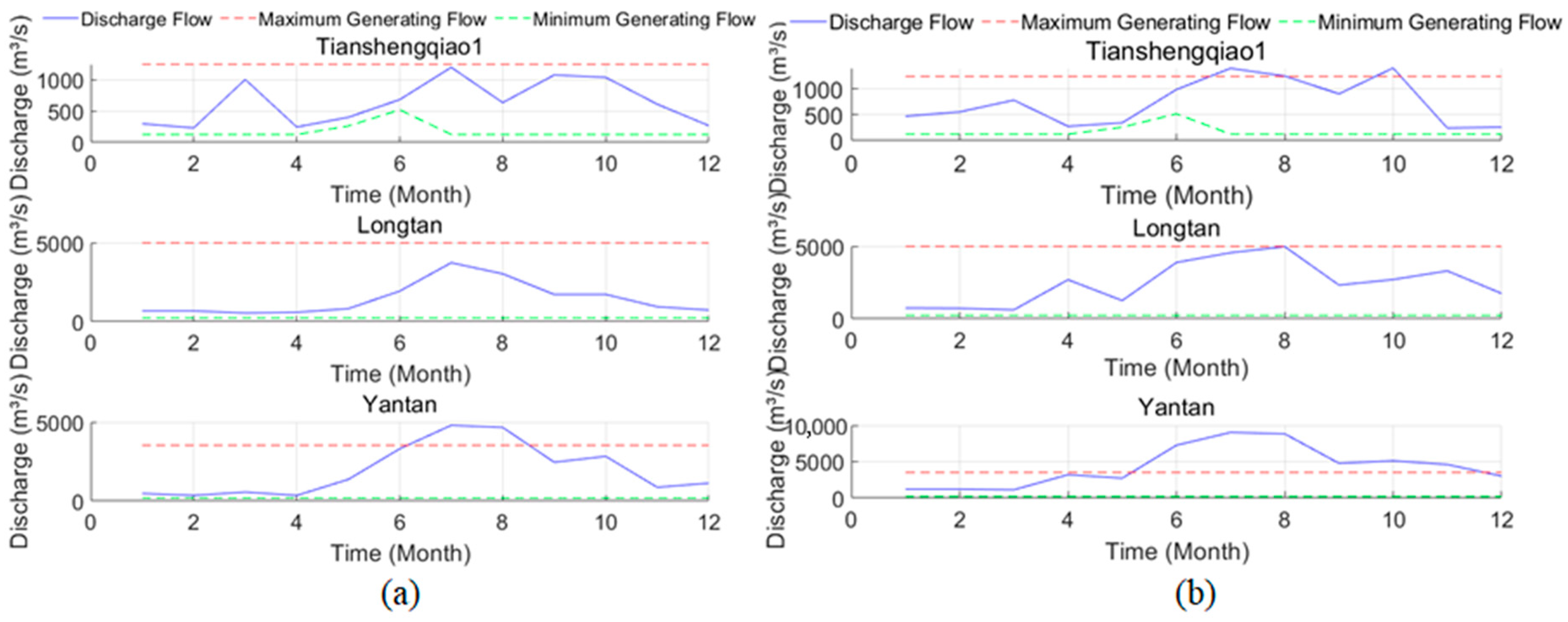
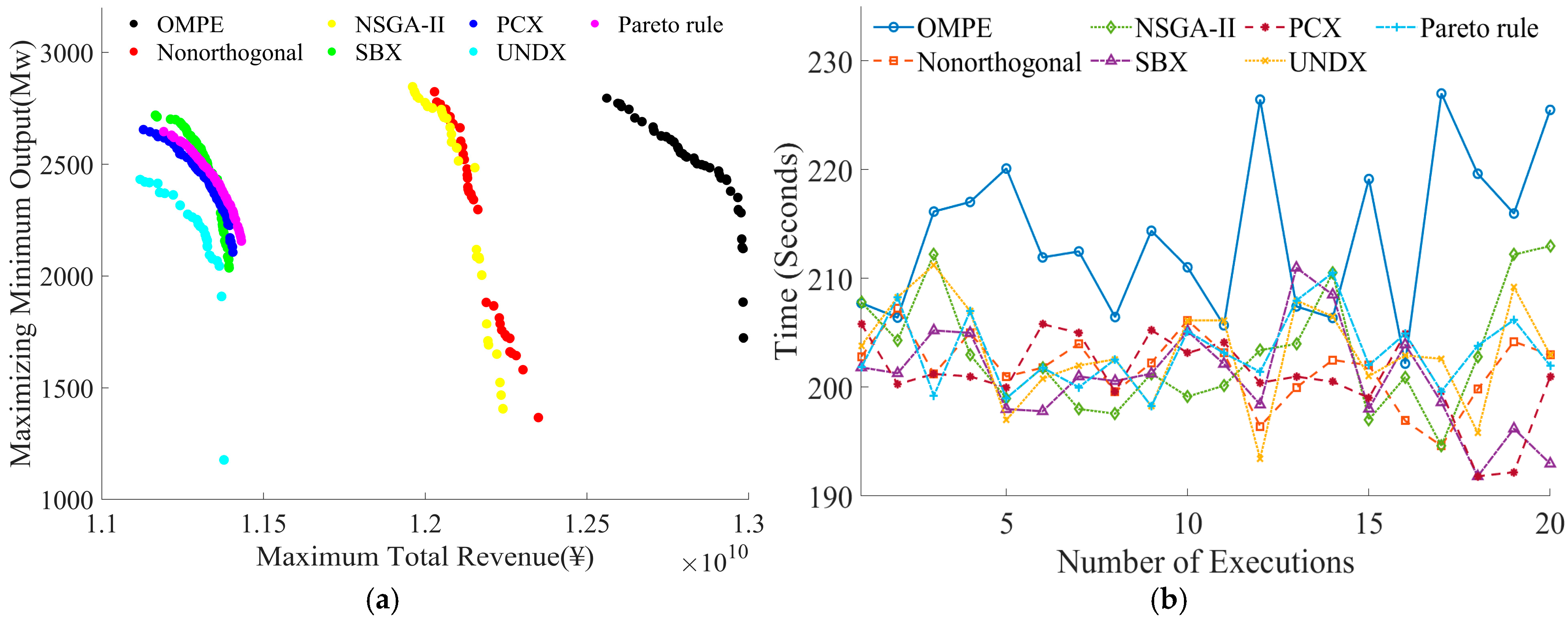
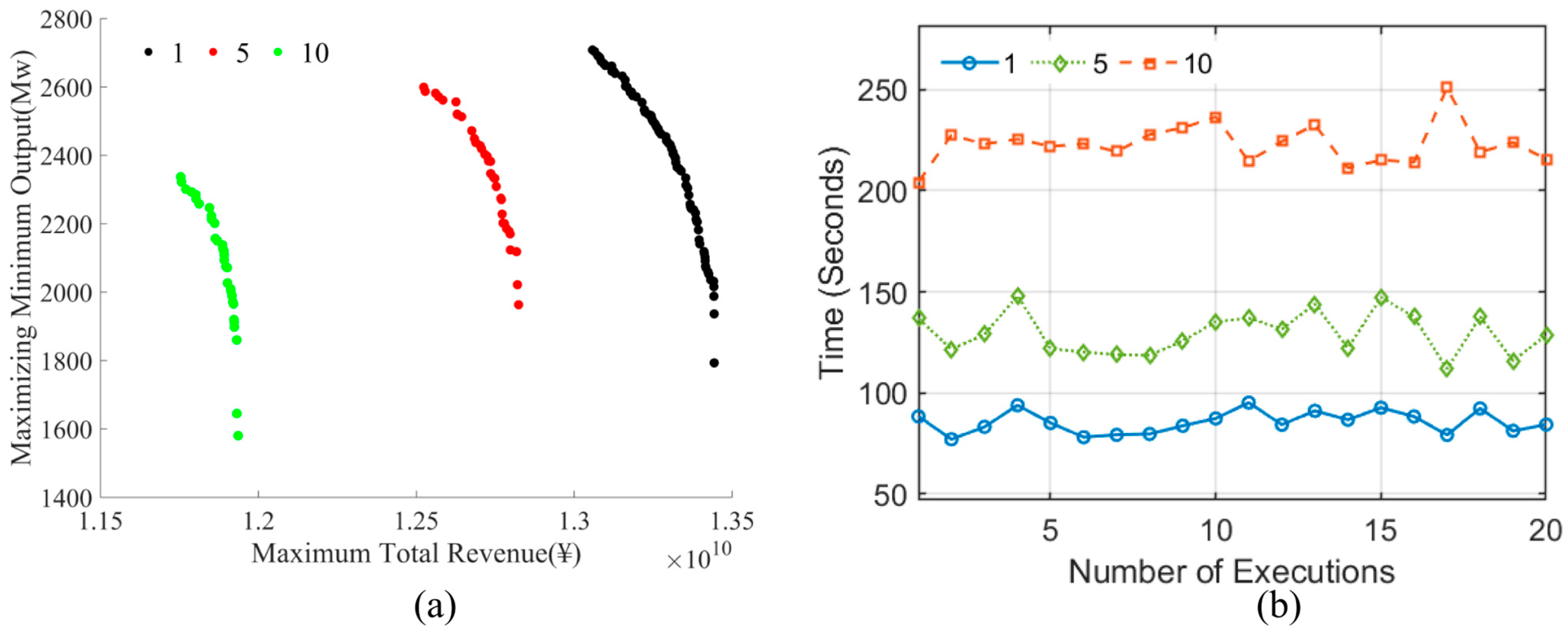
The case study results demonstrate that the proposed approach is effective in capturing the time-based correlation of hydropower, wind, and photovoltaic resources for the Hongshui River cascade system. The scenario generation method successfully reproduces the empirical distributions and temporal correlations observed in the historical data. Furthermore, the optimization model and OMPE algorithm yield feasible and competitive scheduling solutions under the conditions considered, with improvements in total revenue and minimum output compared to NSGA-II. These findings suggest that the integrated framework is a promising tool for long-term scheduling in similar multi-reservoir systems with multi-energy complementarity. Compared to the NSGA-II algorithm, the OMPE proposed in this study shows improvements in total revenue and minimal output by 5.46% and 3.89%, respectively. The comparison results demonstrate that various operational components, including orthogonalization, recombination operators, and dominance rules, have significant impacts on the performance of the OMPE algorithm. Furthermore, the results indicate that different scales of scenarios control the preference of decision makers regarding the economic benefit and risk of the scheduling results, where a larger number of scenarios contributes to a scheduling result with lower risk and economic benefit.

While the proposed framework demonstrates satisfactory performance in the Hongshui River case study, several limitations should be acknowledged regarding its generalizability. The case study involves a basin with distinct wet and dry seasons and well-regulated cascade reservoirs. For basins dominated by snowmelt, glacial melt, or highly variable intermittent flows, the framework may require adaptation. In such cases, the assumption of stationary empirical distributions may be less valid. The scenario generation method relies on sufficient historical data to estimate empirical CDFs and correlation matrices. In basins with limited data, alternative approaches may need to be considered, such as parametric distributions or synthetic generation. This study focuses on the long-term scheduling of a multi-energy system, which may be influenced by the restrictions of short-term scheduling. To address this issue, the proposed model can be expanded into a multi-scale optimization framework. This would involve integrating long-term and short-term scheduling with boundary-related constraints.