Compound Flood Socio-Economic Risk Assessment in Klaipėda City for Sustainable and Climate-Resilient Urban Development

Abstract

Extreme hydrometeorological events are occurring more often under climate change, increasing the risk for cities in coastal zones and lower river reaches. Such areas are prone to compound flooding (CF), where flood duration and magnitude are amplified by the combined effects of storm surges, onshore winds, long-term sea-level rise, and increasingly frequent rainfall-driven floods. This study assesses the socio-economic risk of residential neighbourhoods (RNs) along the lower reach of the Danė River in the city of Klaipėda, Lithuania, using a composite socio-economic risk index (CSERI) developed in this study under an extreme flood scenario, if the sea level in the south-eastern Baltic Sea rises by 1 m by the end of the century. The results show a strong relationship between water levels in the Klaipėda Strait and the lower reach of the Danė River, confirming a CF regime, where flood magnitude is driven by the interaction between strait water level and river discharge. The CSERI is based on five risk sub-indices (SIs): the building risk SI, road infrastructure risk SI, population risk SI, economic entities risk SI, and cultural heritage risk SI. The assessment identifies RNs at greatest risk under climate change and anthropogenic pressure and indicates priority areas for adaptation measures to reduce potential socio-economic losses. The proposed CSERI provides a practical decision-support tool for sustainable and climate-resilient urban development in coastal cities.

1. Introduction

Relative sea-level rise driven by climate change is one of the most important factors behind the increasing frequency of extreme events [1], and since the 1960s, these processes have been further intensified by anthropogenic pressure. As a result, long-term sea-level rise increases the probability of coastal flooding. At the regional scale, sea-level rise driven by climate change differs across the Baltic Sea. It is strongest along the southern Baltic Sea coast and decreases towards the north-east, where vertical land movement (land uplift) partly offsets sea-level rise [2]. Moreover, in inhabited coastal areas of the Baltic Sea, climate-related impacts are further amplified by anthropogenic pressure arising from interacting sectors, including transport, industry, economic activity, energy production, and food production [3].

In the Baltic Proper, especially in the southern and south-eastern parts, climate change is evident not only in long-term sea-level rise but also in increasingly frequent extremes, when storm events drive water levels to their highest values [4,5]. Similarly, long-term water level rise has been observed in the Klaipėda Strait [6,7,8], which increases the likelihood of storm surges and extreme flooding in the coastal city of Klaipėda. Along the south-eastern Baltic Sea coast, the mean water level rose by an average of 4.2 mm per year over 1961–2024. Accordingly, the mean water level in the Klaipėda Strait increased by approximately 25 cm over this period.

In the lower reach of the Danė River within the territory of Klaipėda City, typical CFs occur, driven by the interaction of two or more hydrometeorological drivers [9,10,11]. In this area, water levels in the Danė River and the Klaipėda Strait show strong co-variation. Therefore, when developing future hydrometeorological event scenarios, the key drivers include the long-term water level rise in the Klaipėda Strait, extreme storm-driven water level surges, and variations in the Danė River discharge. Although projections of extreme sea levels are subject to substantial uncertainty [12], they remain essential for scenario-based coastal planning. Regional comparisons suggest that increases in the magnitude and recurrence of very high water levels along the Lithuanian coast are projected to be slower than in the eastern Baltic sub-basins [13], but these projections should nevertheless be incorporated when developing coastal inundation scenarios.

Flood probability scenarios support the prioritisation of areas where infrastructure protection and preventive measures should be planned and implemented. Against this background, the study in [14] shows that climate-change drivers need to be effectively integrated into decision-making in the Baltic Sea region. Accordingly, in CF-affected areas, a risk assessment index can serve as an integrated decision-support tool, enabling the planning of urban development and protection measures while accounting for the increasing flood impacts driven by climate change. In conceptual terms, climate change risk can be defined as the interaction between hazard, exposure, and vulnerability [15]. These components are inherently dynamic because they are shaped by changing climatic conditions, urban development, and other anthropogenic changes. Consequently, a risk assessment index should be scenario-based and periodically updated to reliably reflect the changing flood risk distribution across space and time. At the same time, vulnerability assessment in flood risk models is subject to substantial uncertainty because empirical flood damage data are often not collected or are limited [16]. Taken together, these climate-change drivers and risk components (hazard, exposure, and vulnerability) point to the need to develop a decision-support methodology.

Flood risk is shaped by multiple interacting and changing factors, and index-based approaches are therefore increasingly used in practice [17,18] to summarise how risk is distributed across space and time and to support comparison across different spatial scales and contexts [19]. The aim of coastal flood vulnerability assessment is to establish a clear link between theoretical concepts and everyday decision-making. Therefore, the index should be an accessible and practically applicable tool [20]. In practice, index-based approaches are intended to help reduce urban vulnerability in the context of climate change. When constructing integrated flood risk indices, assessment extends beyond flood hazard to include exposure and vulnerability, reflected in population and socio-economic indicators, the built-up structure, and infrastructure (e.g., road networks, buildings, and critical facilities) [17,21]. Flood exposure is defined as “people, property, systems, or other elements present in hazard zones that are thereby subject to potential losses” [22]. Cultural heritage assets are often assessed separately in flood risk studies as a distinct asset category that may incur losses [23,24,25]. Considering their importance for local communities, historical memory, and national identity, it is appropriate to integrate heritage assets into broader socio-economic flood risk assessments as an additional component, ensuring that decision-making and the prioritisation of measures account for all relevant elements. More generally, social vulnerability indices tend to rely on comparable components across different contexts [26]. Consistent with this, based on a methodological review of socio-economic assessment, Samsuddin et al. [27] emphasise that an integrated assessment of socio-economic and environmental impacts should capture both direct and indirect effects.

Flood impacts on residents include not only material losses but also psychological stress and longer-term mental health impacts. Extreme hydrometeorological situations often lead to emotional distress, characterised by symptoms of anxiety, hopelessness, and fear of the future, which can significantly disrupt daily functioning and work capacity. The scientific literature offers various definitions of psychological responses to climate change. However, universally accepted and consistent definitions are still lacking. Terms such as climate anxiety, climate-related concern, environmentally induced stress, ecological grief, and ecological stress are frequently used in the literature. As a result, differing interpretations and variations in definitions are common [28]. Increasing flood frequency in the context of climate change is associated with a higher prevalence of symptoms of anxiety disorders, post-traumatic stress disorder, and depression [29]. In practice, the emotional side of climate change is also reflected in the efforts of researchers, communication specialists, and educators to identify emotions that could encourage pro-environmental behaviour patterns [30]. However, identifying such an indirect impact on residents usually requires population surveys (questionnaires), and such studies are typically expensive and require a complex, interdisciplinary research design. The practices of countries where such questionnaire-based studies with residents living in flood-risk zones have already been conducted (e.g., the Netherlands, Germany, and the United Kingdom) [31,32,33,34,35] can provide a useful methodological basis for planning similar studies in other countries. However, such approaches should be carefully adapted to the specific socio-economic, institutional, and cultural context of each country, as vulnerability patterns and the impacts of climate-related extremes may differ substantially across regions.

In our previous study, we assessed the impact of Baltic Sea sea-level rise on CF risk in Klaipėda City and, based on modelling results, developed an extreme CF scenario [36]. In the present paper, we adopt this scenario as a fixed hazard baseline and focus on exposure and vulnerability by constructing a CSERI for Klaipėda City. The proposed index serves as a decision-support tool to identify priority zones for protection and adaptation measures. It can also be readily updated as new hazard scenarios become available and applied to other locations. The proposed framework supports sustainable urban development by helping planners prioritise adaptation measures, avoid new risk accumulation, and improve resilience in coastal cities.

2. Materials and Methods

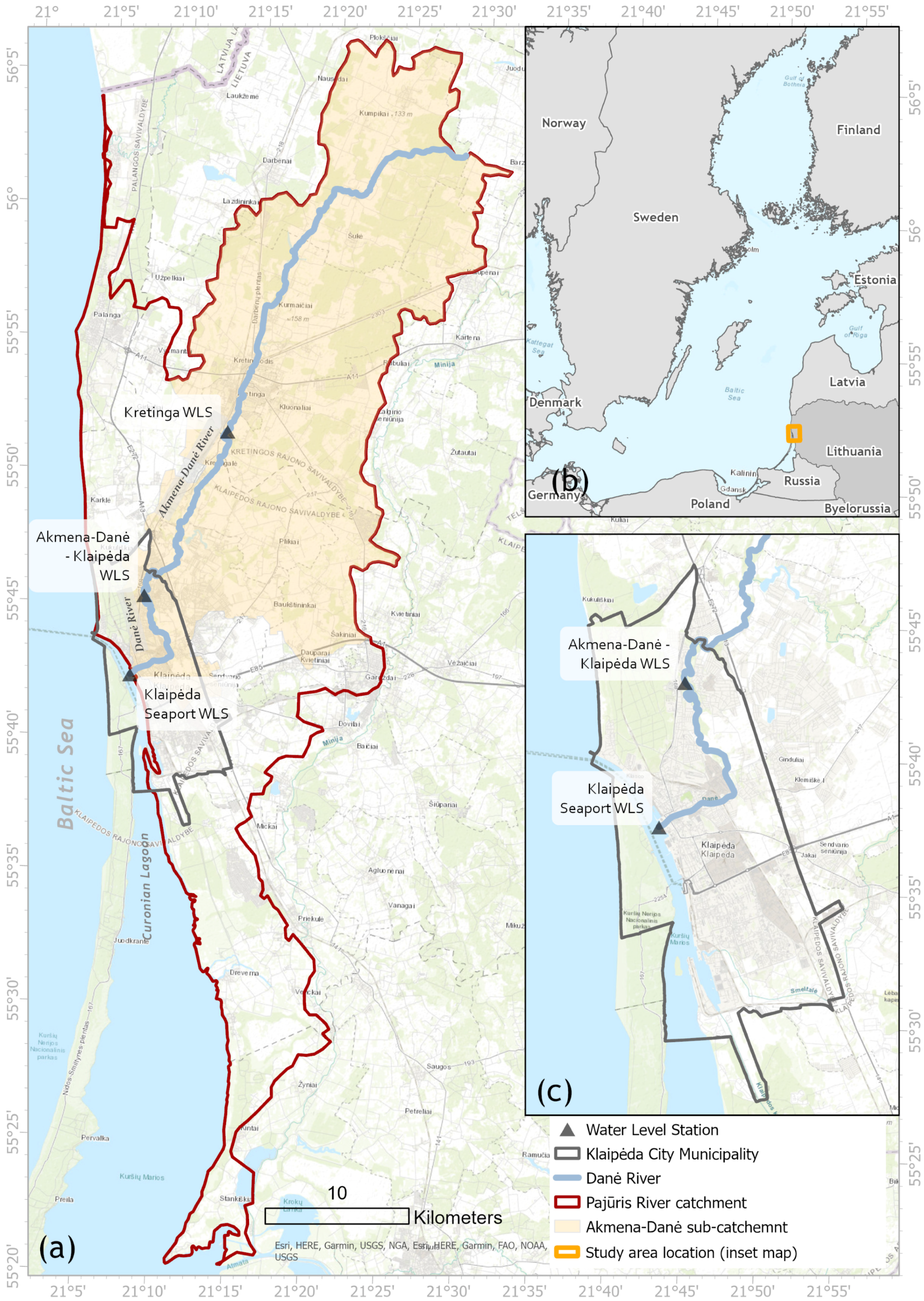
In the city of Klaipėda, where the Akmena–Danė River flows (Figure 1) into the Klaipėda Strait, the hydrological regime of the Pajūris River catchment is shaped not only by river discharge but also by sea-level fluctuations. The Lithuanian Pajūris River catchment covers an area of approximately 2132 km², while the Akmena–Danė River sub-catchment, covering about 580 km², accounts for approximately 27.2% of the total basin area [37]. Although the catchment has no clearly defined main river, the Akmena–Danė sub-catchment is distinguished as a separate sub-catchment [38]. The Pajūris River catchment extends along the Baltic Sea coast and covers almost the entire Lithuanian coastal line, as well as the coastline of the Curonian Lagoon. The lower reaches of the Akmena–Danė River are located in the port city of Klaipėda, and the river flows into the Klaipėda Strait at a distance of approximately 3.8 km from the port gates that connect the strait with the Baltic Sea (author’s GIS calculation using official spatial data in the LKS coordinate system). From its source near Salantai to the lower reaches near Mažieji Žalimai, the river is termed the Akmena, while the downstream section is known as the Danė.

The length of the Akmena–Danė River from its source near Salantai to the Klaipėda Strait is 62.5 km [37], while within the territory of Klaipėda City Municipality, the length of the Danė River reaches about 12.8 km [39]. The mean discharge of the Danė in its lower reaches is 7.6 m³/s; however, large seasonal, rainfall-driven fluctuations are observed, during which the discharge ranges from 0.7 m³/s (minimum) to 90 m³/s (maximum) [40]. In urbanised territories within the cities of Kretinga and Klaipėda, the river is more regulated, while in the middle reaches, a more natural river and valley morphology more often remains. Due to direct interaction with the Baltic Sea and the effects of urbanisation, the Danė is particularly sensitive to hydrological fluctuations and flood processes.

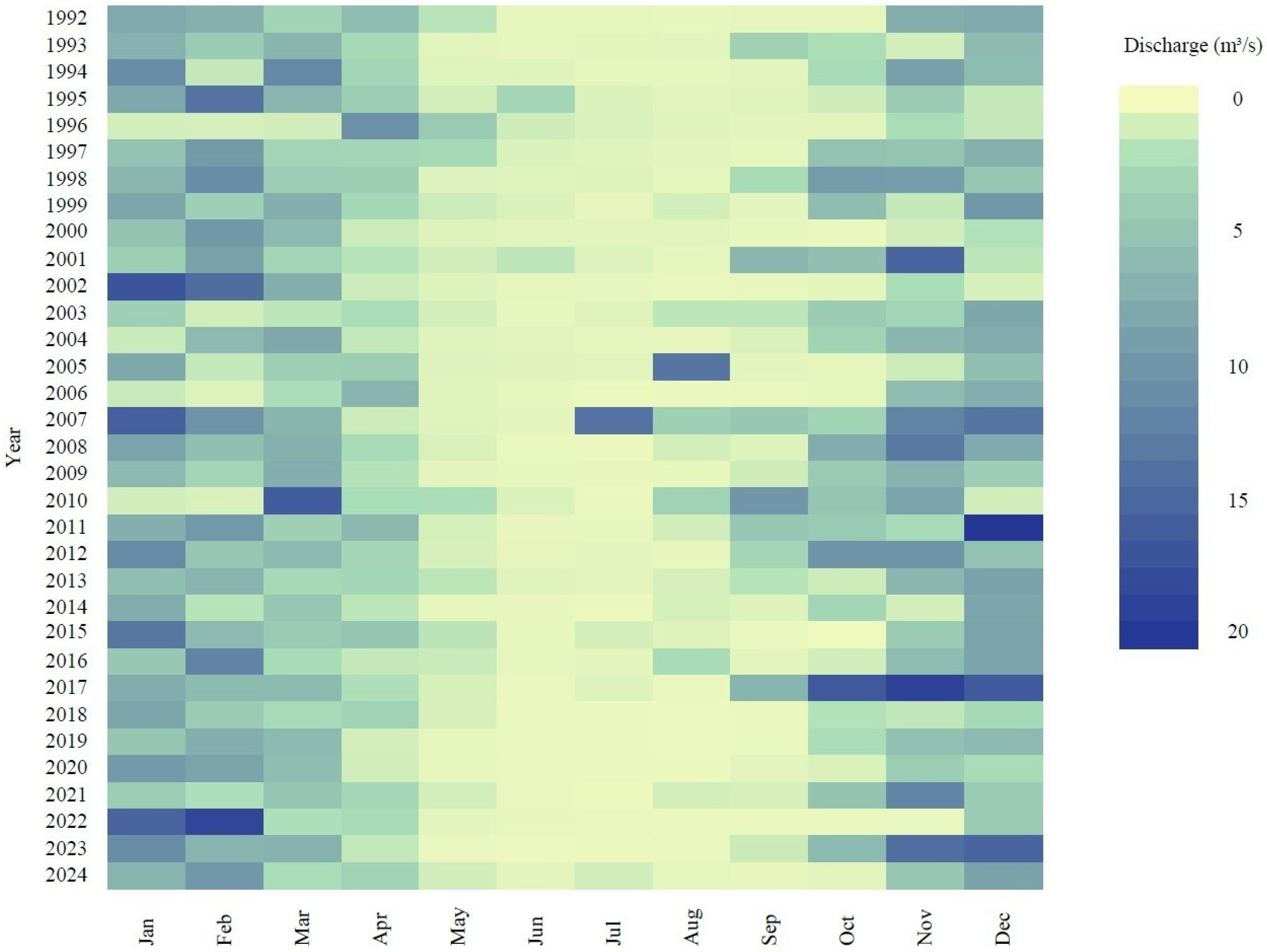
The Danė River is characterised by typical CF driven by rising water levels in the Klaipėda Strait and the Danė discharge. When these two factors act together, the flood extent increases and poses a risk to the city, its infrastructure, and residents. Under these conditions, a backwater effect develops at the river mouth. Due to the water level rise in the strait, river water drains less efficiently into the Curonian Lagoon, causing the river level to rise more rapidly and increasing the extent of inundation. To assess the relationship between water levels in the Danė River and the Klaipėda Strait, water level data for the Danė River and the Klaipėda Strait were used from the Lithuanian Hydrometeorological Service (LHMS; under the Ministry of Environment) for the Klaipėda Seaport and the Akmena–Danė–Klaipėda water-level gauging stations. Daily mean water level values (cm) for 2018–2025 were used. LHMT station data are publicly available from 2022 onwards via the LHMT archive (https://archyvas.meteo.lt; accessed on 17 February 2026). Records for 2018–2021 were obtained from LHMT upon request. To determine the relationship between the daily mean values of these hydrometeorological indicators in 2018–2025, the Pearson correlation coefficient was used. The quality of the regression was assessed using r², the coefficient of determination. The seasonal variation in the mean discharge of the Akmena–Danė River in 1992–2024 was analysed using a colour density diagram. Discharge data were used from the Kretinga WLS. Discharge records for 1992–2024 were obtained from LHMT upon request. The visualisation helped to identify seasonal patterns, periods of extreme discharge, and long-term trends.

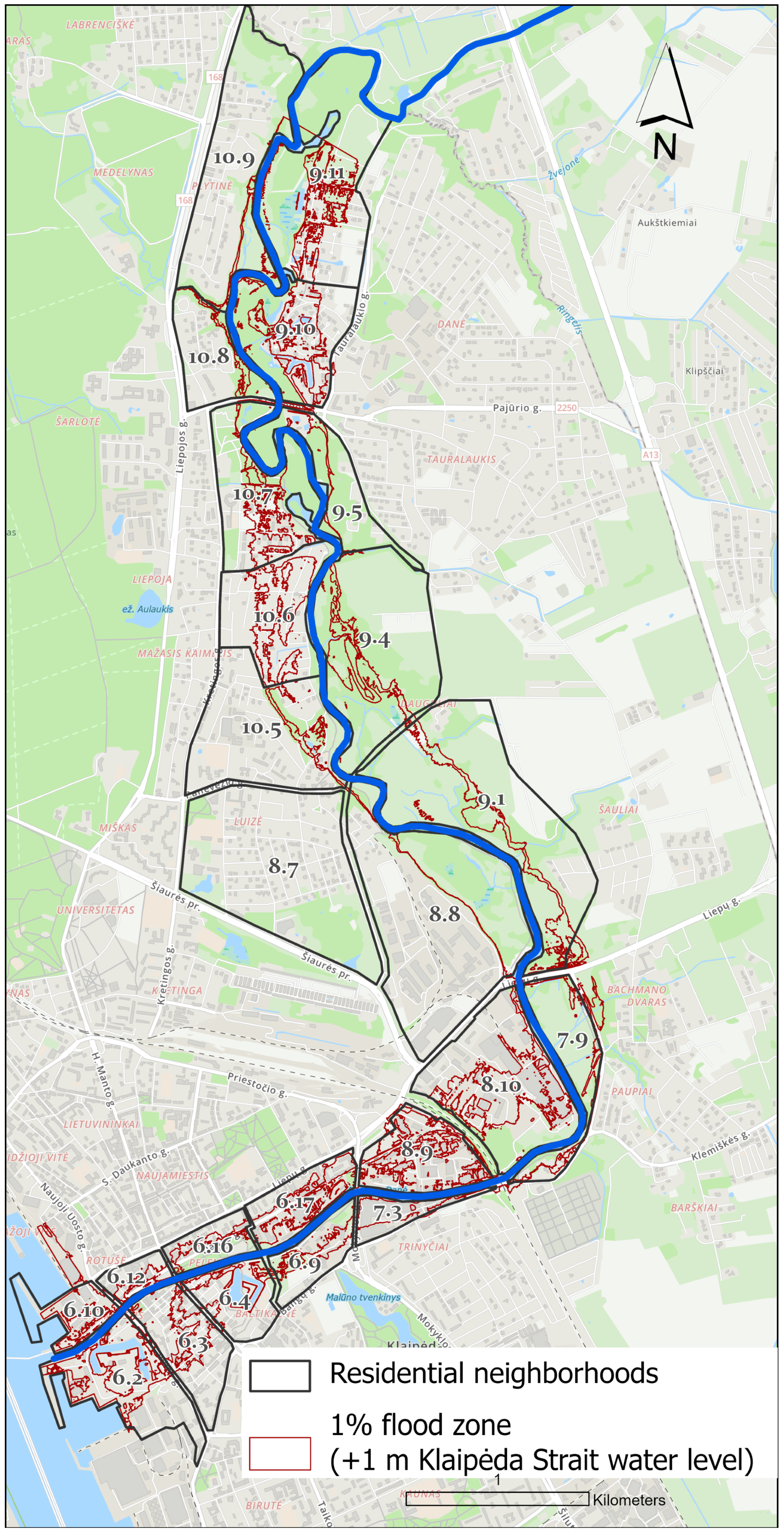
The CF impact on the socio-economic environment of Klaipėda City was assessed using the CSERI calculated at the level of RN located adjacent to the Danė River (Figure 2). The assessment considered five impact domains: buildings, infrastructure (roads), residents, business entities, and cultural heritage entities located within the flood risk zone.

The CSERI was developed based on the understanding that flood risk arises from the interaction between hazard, exposure, and vulnerability [41,42]. In this study, hazard was defined by the extreme compound flood scenario, while the analysis focused on the exposure of socio-economic elements located within the flooded area. Following the concept of exposure, five impact domains were selected for assessment at the RN level: buildings, roads, residents, business entities, and cultural heritage entities. Vulnerability indicators were not included in the index separately.

The impact domains were selected to represent socio-economic elements of the urban system that may be directly or indirectly affected during flooding. Buildings reflect potential direct physical damage, roads represent disruptions to mobility, accessibility, and urban connectivity [43,44], residents capture potential population exposure within the flood-affected area and possible implications for human safety [45,46], business entities indicate possible impacts on economic activity and service continuity [47], and cultural heritage entities reflect the vulnerability of historically and socially valuable assets, which are receiving increasing attention in flood risk assessment [48].

The extreme flood risk zone was defined based on the results of previous studies [36]. In the present study, this scenario served as a spatial reference for comparing neighbourhood-level flood risk, while direct validation against observed socio-economic damage data was beyond the scope of the analysis. The extreme scenario is based on the assumption that the water level in the Klaipėda Strait increases by 1 m and reaches 3 m. As defined in the previous study, this scenario represents an extreme-case flood extent under maximum spring flood conditions and does not separately incorporate river-discharge change. RN boundaries were digitised by the authors from the Klaipėda City Master Plan [40] and used as the main spatial aggregation unit. For each domain, the number of objects within the extreme flood zone was determined using ArcGIS Pro by spatially overlaying the object layers with the flood-zone polygon.

The number of buildings and the length of roads in the flood zone were calculated from the 2021 georeferenced base cadastre dataset. The number of business entities [49] and cultural heritage objects [50] was obtained from the open data services of the Lithuanian State Data Agency. Object layers were intersected with RN boundaries and the extreme flood scenario extent to count objects within the flood zone per RN. Population in each analysed RN was estimated using the 2021 Population and Housing Census data in a regular 100 × 100 m GRID format [51]. The 100 × 100 m population GRID layer was overlaid with residential neighbourhood (RN) boundaries, retaining cells that were fully within an RN or had more than 50% of their area within it. Thus, population values from the selected cells were summed for each RN. To assess flood impacts, the population living in GRID cells within the extreme flood scenario extent was summed for each RN. These values were used in the CSERI calculations.

To assess the spatial distribution and concentration of different elements (buildings, business entities, cultural heritage entities, and roads), kernel density estimation (KDE) was applied using consistent parameters (15 m cell size; 200 m search radius), and the resulting density surfaces were used to visualise their overlap with the extreme flood scenario extent. The selected parameters were intended to preserve sufficient spatial detail for urban-scale analysis while avoiding an overly fragmented density surface. A 15 m cell size was used to retain fine-scale spatial variation, whereas a 200 m search radius allowed local concentrations of exposed elements to be generalised at the RN scale. The same parameter set was applied across domains to ensure comparability of the resulting density surfaces. KDE was performed using a fixed-bandwidth quartic (Epanechnikov) kernel function, with distances computed using the planar method [52]. The building polygon layer was converted to point data by calculating the geometric centroid of each building for the density analysis. This approach is commonly used to analyse the concentration of urban structures when assessing the spatial distribution of objects [53,54]. Road network density was estimated using KDE without barriers, as the aim was to capture overall infrastructure distribution. The population GRID data are already spatially aggregated and area-normalised (people/km²), so no additional KDE was applied. Population exposure was assessed by analysing the intersection of GRID cells with the extreme flood scenario extent. The KDE results were used for spatial interpretation, whereas risk classification was based on RN-level aggregated values. All spatial analyses were performed in ArcGIS Pro (3.6.0, Esri, Redlands, CA, USA) in the Lithuanian national coordinate reference system LKS94 (EPSG:3346).

Separate risk SIs were developed for the selected assessment domains (buildings, infrastructure, population, business entities, and cultural heritage entities) and then combined into an overall CSERI. For all domains, the RN served as the main aggregation unit, whereas impact magnitude was expressed using the domain-specific measurement unit: flooded buildings (count), flooded roads (km), affected population (number of residents), flooded business entities (count), and flooded cultural heritage entities (count). Each risk SI consisted of two components: (1) impact magnitude and (2) relative exposure, defined as the share (%) of flooded elements relative to the total amount of the domain within the RN. Magnitude captures absolute impact, while relative exposure captures the proportional impact within the RN. Together, these two components allowed both the absolute extent of impact and its relative severity within each RN to be taken into account across all assessment domains.

A quartile-based approach was used for categorising impact magnitude for each assessment domain. Quartile thresholds were defined as the empirical 25th, 50th, and 75th percentiles (Q25–Q75) of the distribution of non-zero exposure values across RNs (

Table 1. Quartile thresholds (Q1–Q3) used for categorising impact magnitude under the extreme flood scenario.

Quartile	Buildings	Roads (km)	Population	Business Entities	Cultural Heritage Entities
Q1	16	0.7	66	4	3
Q2	33	1.5	154	19	5
Q3	69	2.1	303	30	7

). These thresholds were calculated separately for each domain using RN-level aggregated values. The underlying data are provided in

Table A1. Building risk sub-index for RNs within extreme flood scenario.

RN Name	Total Number of Buildings in the RN	Impact Magnitude			Relative Exposure
		Number of Flooded Buildings	Impact Magnitude Level	Impact Magnitude Score	Flooded Buildings (% of Total Buildings in the RN)	Relative Exposure Level	Relative Exposure Score	Building Risk SI
6.2 Piliavietės	43	27	medium	2	63	high	3	3
6.3 Senamiesčio	229	149	extreme	4	65	high	3	4
6.4 Bastioninių įtvirtnimų	60	25	medium	2	42	medium	2	2
6.9 Pelenyno	47	28	medium	2	60	high	3	3
6.10 Šiaurės rago	17	16	low	1	94	extreme	4	3
6.12 Rotušės	19	12	low	1	63	high	3	2
6.16 Senosios elektrinės I	28	16	low	1	57	high	3	2
6.17 Senosios elektrinės II	74	52	high	3	70	high	3	3
7.3 Joniškės III	5	4	low	1	80	extreme	4	3
7.9 Upės uosto	23	19	medium	3	83	extreme	4	4
8.9 Mažosios lankos	79	79	extreme	4	100	extreme	4	4
8.10 Luizės dvaro	67	39	high	3	58	high	3	3
8.7 Karališkosios giraitės	538	0	none	0	0	none	0	0
8.8 Paupių pievos	156	0	none	0	0	none	0	0
9.1 Daugulių	18	0	none	0	0	none	0	0
9.4 Luizės ąžuolo I	0	0	none	0	0	none	0	0
9.5 Luizės ąžuolo II	25	5	low	1	20	low	1	1
9.10 Dvaro slėnio I	153	92	extreme	4	60	high	3	4
9.11 Dvaro slėnio II	116	47	high	3	41	medium	2	3
10.5 Miestiečių laukų I	371	74	extreme	4	20	low	1	3
10.6 Miestiečių laukų II	563	408	extreme	4	72	high	3	4
10.7 Miestiečių laukų III	68	44	high	3	65	high	3	3
10.8 Didžiojo Tauralaukio I	102	0	none	0	0	none	0	0
10.9 Didžiojo Tauralaukio II	292	0	none	0	0	none	0	0

,

Table A2. Infrastructure risk SI for RNs within extreme flood scenario.

RN Name	Total Road Length in RN (km)	Impact Magnitude			Relative Exposure
		Flooded Road Length (km)	Impact Magnitude Level	Impact Magnitude Score	Flooded Roads (% of Total Length) in the RN)	Relative Exposure Level	Relative Exposure Score	Road Infrastructure Risk SI
6.2 Piliavietės	1.1	1.1	medium	2.0	100	extreme	4	3
6.3 Senamiesčio	4.3	3.8	extreme	4.0	88	extreme	4	4
6.4 Bastioninių įtvirtnimų	2.6	1.5	medium	2.0	57	high	3	3
6.9 Pelenyno	0.9	0.9	medium	2.0	100	extreme	4	3
6.10 Šiaurės rago	0.6	0.6	low	1.0	100	extreme	4	3
6.12 Rotušės	0.3	0.3	low	1.0	100	extreme	4	3
6.16 Senosios elektrinės I	1.7	1.7	high	3.0	100	extreme	4	4
6.17 Senosios elektrinės II	0.8	0.8	medium	2.0	100	extreme	4	3
7.3 Joniškės III	0.5	0.5	low	1.0	100	extreme	4	3
7.9 Upės uosto	0.6	0.6	low	1.0	100	extreme	4	3
8.9 Mažosios lankos	2.7	2.7	extreme	4.0	100	extreme	4	4
8.10 Luizės dvaro	4.2	3.9	extreme	4.0	93	extreme	4	4
8.7 Karališkosios giraitės	7.5	0.0	none	0.0	0	none	0	0
8.8 Paupių pievos	7.5	1.7	high	3.0	23	medium	2	3
9.1 Daugulių	1.2	0.0	none	0.0	0	none	0	0
9.4 Luizės ąžuolo I	0.7	0.0	none	0.0	0	none	0	0
9.5 Luizės ąžuolo II	0.6	0.1	low	1.0	17	low	1	1
9.10 Dvaro slėnio I	1.4	1.1	medium	2.0	76	high	3	3
9.11 Dvaro slėnio II	2.2	1.5	medium	2.0	67	high	3	3
10.5 Miestiečių laukų I	5.7	2.1	high	3.0	37	medium	2	3
10.6 Miestiečių laukų II	5.0	4.0	extreme	4.0	80	extreme	4	4
10.7 Miestiečių laukų III	3.9	2.1	high	3.0	54	high	3	3
10.8 Didžiojo Tauralaukio I	0.9	0.0	none	0.0	0	none	0	0
10.9 Didžiojo Tauralaukio II	2.6	0.0	none	0.0	0	none	0	0

,

Table A3. Population risk SI for RNs within extreme flood scenario.

RN Name	Number of Population in the RN	Impact Magnitude			Relative Exposure
		Flooded Population (Count)	Impact Magnitude Level	Impact Magnitude Score	Flooded Population (% of Total Population in the RN)	Relative Exposure Level	Relative Exposure Score	Population Risk SI
6.2 Piliavietės	0	0	none	0	0	none	0	0
6.3 Senamiesčio	1649	788	extreme	4	48	medium	2	3
6.4 Bastioninių įtvirtnimų	479	242	high	3	51	high	3	3
6.9 Pelenyno	196	0	none	0	0	none	0	0
6.10 Šiaurės rago	0	0	none	0	0	none	0	0
6.12 Rotušės	455	192	high	3	42	medium	2	3
6.16 Senosios elektrinės I	541	382	extreme	4	71	high	3	4
6.17 Senosios elektrinės II	349	76	high	2	22	medium	2	2
7.3 Joniškės III	7	0	none	0	0	none	0	0
7.9 Upės uosto	27	14	low	1	52	high	3	2
8.9 Mažosios lankos	0	0	none	0	0	none	0	0
8.10 Luizės dvaro	12	0	none	0	0	none	0	0
8.7 Karališkosios giraitės	11,407	0	none	0	0	none	0	0
8.8 Paupių pievos	91	0	none	0	0	none	0	0
9.1 Daugulių	8	0	none	0	0	none	0	0
9.4 Luizės ąžuolo I	0	0	none	0	0	none	0	0
9.5 Luizės ąžuolo II	23	5	low	1	22	medium	2	2
9.10 Dvaro slėnio I	181	116	medium	2	64	high	3	3
9.11 Dvaro slėnio II	76	34	low	1	45	medium	2	2
10.5 Miestiečių laukų I	2035	99	medium	2	5	low	1	2
10.6 Miestiečių laukų II	390	277	high	3	71	high	3	3
10.7 Miestiečių laukų III	819	669	extreme	4	82	extreme	4	4
10.8 Didžiojo Tauralaukio I	164	0	none	0	0	none	0	0
10.9 Didžiojo Tauralaukio II	546	0	none	0	0	none	0	0

,

Table A4. Business entities risk SI for RNs within extreme flood scenario.

RN Name	Total Number of Business Entities in the RN	Impact Magnitude			Relative Exposure
		Number of Flooded Business Entities	Impact Magnitude Level	Impact Magnitude Score	Flooded Business Entities (% of Total Business Entities in the RN)	Relative Exposure Level	Relative Exposure Score	Business Entities Risk SI
6.2 Piliavietės	41	18	medium	2	44	medium	2	2
6.3 Senamiesčio	267	156	extreme	4	58	high	3	4
6.4 Bastioninių įtvirtnimų	102	30	high	3	29	medium	2	3
6.9 Pelenyno	21	5	medium	2	24	medium	2	2
6.10 Šiaurės rago	5	4	low	1	80	extreme	4	3
6.12 Rotušės	87	30	high	3	34	medium	2	3
6.16 Senosios elektrinės I	68	34	extreme	4	50	medium	2	3
6.17 Senosios elektrinės II	97	27	high	3	28	medium	2	3
7.3 Joniškės III	2	0	none	0	0	none	0	0
7.9 Upės uosto	4	2	low	1	50	medium	2	2
8.9 Mažosios lankos	38	38	extreme	4	100	extreme	4	4
8.10 Luizės dvaro	33	0	none	0	0	none	0	0
8.7 Karališkosios giraitės	85	0	none	0	0	none	0	0
8.8 Paupių pievos	96	0	none	0	0	none	0	0
9.1 Daugulių	13	0	none	0	0	none	0	0
9.4 Luizės ąžuolo I	0	0	none	0	0	none	0	0
9.5 Luizės ąžuolo II	4	0	none	0	0	none	0	0
9.10 Dvaro slėnio I	18	7	medium	2	39	medium	2	2
9.11 Dvaro slėnio II	7	3	low	1	43	medium	2	2
10.5 Miestiečių laukų I	87	2	low	1	2	low	1	1
10.6 Miestiečių laukų II	24	19	medium	2	79	extreme	4	3
10.7 Miestiečių laukų III	46	26	high	3	57	high	3	3
10.8 Didžiojo Tauralaukio I	15	0	none	0	0	none	0	0
10.9 Didžiojo Tauralaukio II	26	0	none	0	0	none	0	0

and

Table A5. Cultural heritage entities risk SI for RNs within extreme flood scenario.

RN Name	Total Number of Cultural Heritage Entities in the RN	Impact Magnitude			Relative Exposure
		Number of Flooded Cultural Heritage Entities	Impact Magnitude Level	Impact Magnitude Score	Flooded Cultural Heritage Entities (% of Total Cultural Heritage Entities in the RN)	Relative Exposure Level	Relative Exposure Score	Cultural Heritage Entities Risk SI
6.2 Piliavietės	11	8	extreme	4	73	high	3	4
6.3 Senamiesčio	46	27	extreme	4	59	high	3	4
6.4 Bastioninių įtvirtnimų	9	3	low	1	33	medium	2	2
6.9 Pelenyno	2	0	none	0	0	none	0	0
6.10 Šiaurės rago	2	2	low	1	100	extreme	4	3
6.12 Rotušės	0	0	none	0	0	none	0	0
6.16 Senosios elektrinės I	4	0	none	0	0	none	0	0
6.17 Senosios elektrinės II	5	5	high	3	100	extreme	4	4
7.3 Joniškės III	0	0	none	0	0	none	0	0
7.9 Upės uosto	0	0	none	0	0	none	0	0
8.9 Mažosios lankos	4	4	medium	2	100	extreme	4	3
8.10 Luizės dvaro	0	0	none	0	0	none	0	0
8.7 Karališkosios giraitės	0	0	none	0	0	none	0	0
8.8 Paupių pievos	0	0	none	0	0	none	0	0
9.1 Daugulių	0	0	none	0	0	none	0	0
9.4 Luizės ąžuolo I	0	0	none	0	0	none	0	0
9.5 Luizės ąžuolo II	0	0	none	0	0	none	0	0
9.10 Dvaro slėnio I	0	0	none	0	0	none	0	0
9.11 Dvaro slėnio II	0	0	none	0	0	none	0	0
10.5 Miestiečių laukų I	0	0	none	0	0	none	0	0
10.6 Miestiečių laukų II	0	0	none	0	0	none	0	0
10.7 Miestiečių laukų III	0	0	none	0	0	none	0	0
10.8 Didžiojo Tauralaukio I	0	0	none	0	0	none	0	0
10.9 Didžiojo Tauralaukio II	2	0	none	0	0	none	0	0

. RNs with no objects in an assessment domain were assigned “no impact” (score 0) prior to categorisation. For the remaining (non-zero) values, impact magnitude was categorised as follows: score 1 (0 < x ≤ Q25), score 2 (Q25 < x ≤ Q50), score 3 (Q50 < x ≤ Q75), and score 4 (x > Q75). This avoided artificially distorting quartile thresholds due to many zero values.

Relative exposure was categorised using the same risk level and score: 0 = none, 1 = low (≤20%), 2 = medium (21–50%), 3 = high (51–79%), and 4 = extreme (≥80%). For each domain, the risk SI was calculated as the mean of the magnitude and relative exposure scores. The five risk SIs were then combined into the CSERI as a weighted sum of risk SIs:

$$CSERI=\sum _{j=1}^5{w}_{\_j}\cdot S{I}_{\_j}$$

The weights assigned to the five risk SIs sum to 1 (∑w = 1), so CSERI can be interpreted as a weighted mean of the risk SIs, where $S{I}_{\_j}$ is the risk sub-index for domain $j$, and $w_{\_j}$ is its weight. The weighting schemes were designed to represent alternative planning priorities rather than a single universally optimal weighting solution. Four scenarios were applied (

Table 2. Risk SI weighting schemes for CSERI scenarios (equal weight, human safety, and balanced urban functioning).

	Indices	Equal Weight	Human Safety	Balanced Urban Functioning
Risk Subindex Value
Buildings		0.20	0.20	0.20
Roads		0.20	0.20	0.25
Population		0.20	0.35	0.25
Business entities		0.20	0.15	0.15
Cultural heritage entities		0.20	0.10	0.15

Note: In the extreme-case scenario, CSERI was defined as the maximum risk SI value within the RN, i.e., $CSERI=\mathrm{m}\mathrm{a}\mathrm{x}(S{I}_1,S{I}_2,S{I}_3,S{I}_4,S{I}_5)$.

): the first three use alternative weight sets in the weighted-sum formulation, whereas the fourth applies an extreme-case rule in which CSERI is defined by the largest risk SI value:

$$\mathrm{C}\mathrm{S}\mathrm{E}\mathrm{R}\mathrm{I}=\mathrm{m}\mathrm{a}\mathrm{x}\left(\mathrm{S}{\mathrm{I}}_1,\mathrm{S}{\mathrm{I}}_2,\mathrm{S}{\mathrm{I}}_3,\mathrm{S}{\mathrm{I}}_4,\mathrm{S}{\mathrm{I}}_5\right)$$

The first three scenarios reflect different decision-making perspectives on socio-economic flood risk, while the fourth scenario represents a conservative extreme-case interpretation.

In the equal-weight scenario, all domains were assigned the same importance, and none was treated as less important. In the human safety scenario, the population risk SI received the highest weight, reflecting the priority given to the protection of residents and the reduction of direct social impacts during flood events. Buildings and roads were each assigned a weight of 0.20, whereas business entities and cultural heritage entities were given lower weights of 0.15 and 0.10, respectively. This weighting structure reflects a decision-making perspective in which human safety is prioritised over economic and cultural losses. The balanced urban functioning scenario emphasised the importance of infrastructure for mobility. Therefore, road infrastructure and population were assigned the highest weights (0.25 each). These two domains reflect social impacts and the critical function of urban infrastructure, including access to services and residents’ daily mobility. Together, they represent the continuity of everyday urban functioning during flood events. Buildings, as an indicator of material losses and vulnerability of the residential environment, were weighted at 0.20. The business entity and cultural heritage risk SIs were each assigned a weight of 0.15 to incorporate economic vitality and the preservation of cultural value. The fourth scenario provides a conservative estimate by setting CSERI to the highest risk SI value in the RN.

CSERI values were analysed on a continuous 0–4 scale, where 0 indicates no risk and higher values indicate increasing risk up to the theoretical maximum of 4 (extreme risk). For interpretation and cartographic visualisation, CSERI was additionally grouped into five categories using the following thresholds: 0 = none, 0.01–1.00 = low, 1.01–2.00 = medium, 2.01–3.00 = high, and 3.01–4.00 = extreme. In the comparative analysis, areas were assessed using the continuous CSERI values without assigning discrete risk categories to avoid ambiguity at category boundaries and to maintain sensitivity to spatial differences.

The proposed framework provides a basis for assessing whether planned urban development decisions are aligned with sustainable and climate-resilient land-use planning, and for identifying the socio-economic losses that may result if these principles are ignored. In the context of spatial planning and urban development, projected population [55] and planned residential development areas were analysed. This information was used as contextual material to support the interpretation of results and to discuss the relevance of flood risk management measures.

During the preparation of this manuscript, the authors used generative AI tools to assist with translation and language editing of the text. The authors reviewed and edited the output and take full responsibility for the content of the publication.

3. Results

3.1. Compound Flood Drivers: Strait Water Level and Danė River Discharge

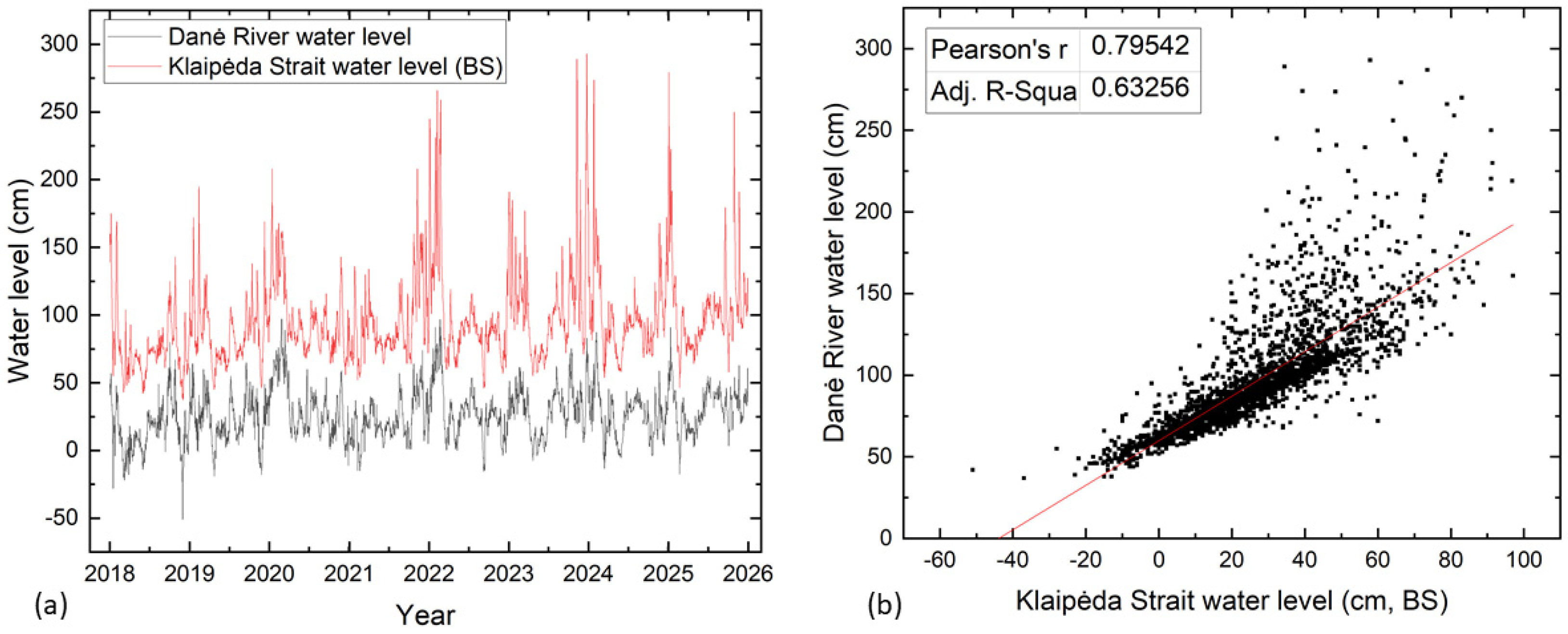
The Danė River water level in its lower reach is strongly influenced by the Klaipėda Strait water level, and when combined with increased Danė (Akmena–Danė) discharge, this amplifies water-level rise and flood risk. This is confirmed by the comparison of daily mean water levels in the Danė River and the Klaipėda Strait for 2018–2025 (Figure 3a). Because the Danė WLS station is located approximately 9.5 km from the Klaipėda Strait WLS station, the time series reflects water-level dependence along the lower Danė reach, covering most of the Klaipėda City area. Both the Danė River and the Klaipėda Strait water levels show large variability and frequent rapid rises. Changes in the Klaipėda Strait water level indicate sensitivity to wind-driven surges [7], whereas fluctuations in the Danė River water level depend both on these surges in the strait and on river discharge. The time series shows that rises in the Danė River water level often coincide with rises in the Klaipėda Strait water level, indicating a strong linkage between marine-driven surges and water-level increases in the Danė River. When one or more additional hydrometeorological drivers coincide—most notably increased river discharge, often following intense precipitation—compound flooding can occur, allowing the Danė River water level to reach extreme values.

The Pearson correlation coefficient between daily water levels in the Klaipėda Strait and the Danė River for 2018–2025 indicates a strong relationship (r = 0.80) (Figure 3b). The adjusted coefficient of determination (Adj. R²) was 0.63, indicating that approximately 63% of the variability in one variable can be explained by the other. Therefore, storm-driven water-level rise contributes to flood formation and increases the potentially vulnerable area of the city. Although the influence of Danė River discharge and precipitation on flooding was not analysed in this study, a nearly 2.5 m rise in the Danė River water level was recorded in November 2017 during a period of heavy rainfall. Urban stormwater drainage capacity influenced flood severity. This highlights the need for an integrated assessment of flood drivers and for identifying weak points in the flood resilience of coastal cities. Such studies would facilitate future adaptation to the potential adverse impacts of storm-driven flooding, enable a more accurate assessment of socio-economic losses, and help mitigate consequences and reduce or avoid socio-economic damage.

Flood formation, particularly during extreme events, is driven not only by storm surges in the Klaipėda Strait associated with water-level rise but also by catchment hydrological conditions, including river discharge, precipitation, and snowmelt. The monthly distribution of mean Akmena–Danė River discharge for 1992–2024 exhibits strong seasonality (Figure 4). The highest discharges are typically recorded in winter and early spring. These periods coincide with more intense cyclonic activity in the southeastern Baltic region [56]. However, exceptional cases also occur. For example, unusually high discharge was recorded in August 2005, and in 2017, the discharge remained higher than usual from September through the end of the year. Although the overall seasonal pattern in discharge is clear, recurring high-flow periods at other times of the year indicate that flood hazard and risk may be relevant across multiple months.

3.2. Risk Sub-Indices

3.2.1. Buildings Risk SI

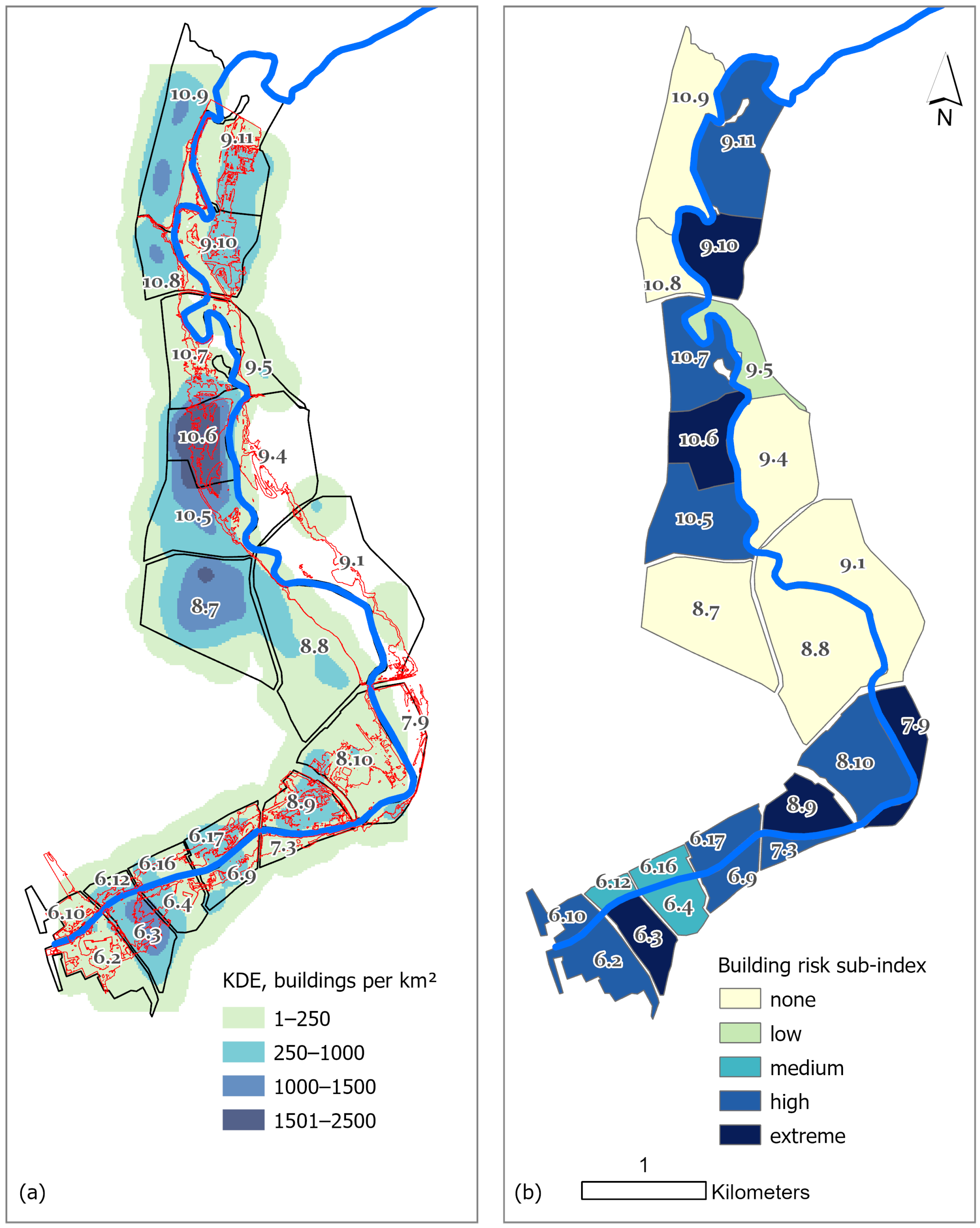
By total building count, the highest values were identified in several northern residential neighbourhoods (Table A1). However, building-related flood risk depends on the overlap between built-up areas and the modelled flood extent. Accordingly, some densely built neighbourhoods show negligible building exposure because their buildings fall outside the flood zone, while some low-density neighbourhoods contain no buildings at all. Among the 24 analysed RNs, 13 have fewer than 100 buildings, and the built environment is spatially uneven. The highest building-related flood risk emerges where dense building concentrations coincide with flood zones, particularly in the Old Town and the northern part of Klaipėda (Figure 5a).

Therefore, building-related flood risk is summarised here using the building risk SI, which integrates impact magnitude (the number of flooded buildings) and relative exposure (the share of flooded buildings relative to the total building count in the RN). In the first step, the impact magnitude was assessed as the number of flooded buildings under the extreme flood scenario. In total, six RNs were categorised as non-exposed because they contain no buildings or their buildings fall outside the flood zone under the extreme flood scenario. The remaining RNs were grouped into four magnitude categories using the thresholds reported in Table 1: low (1–16 flooded buildings), medium (17–33), high (34–68), and extreme (≥69). In the extreme categories, the number of flooded buildings ranged from 74 to 408.

Based on relative exposure (the share of flooded buildings relative to the total building count), four RNs were categorised as extreme risk, with 80–100% of buildings flooded (Table A1). Under this indicator, 10 RNs show high risk, two show medium risk, two show low risk, and six RNs show no risk. It is important to interpret building-related flood risk in a combined way, because the two indicators can place the same RN in different risk categories. For example, in RN 6.3, 149 buildings could be flooded, representing 65% of the total building count, which corresponds to high risk based on relative exposure. In RN 8.9, 79 buildings would be flooded, but this equals 100% of all buildings, placing it in the extreme-risk category. In RN 10.5, 74 buildings are flooded, yet they represent only 20% of the total, so relative exposure indicates low risk, even though the flooded-building count assigns the RN to a higher risk group. These examples show that one indicator reflects absolute impact magnitude, whereas the other captures the proportional intensity of flooding within an RN. The building risk SI was calculated as the mean of the two component scores, and the final risk level was assigned by rounding the risk SI value to the nearest integer. Overall, the RNs were distributed across risk levels as follows: five extreme, nine high, three medium, one low, and six with no identified risk (Figure 5b).

3.2.2. Road Infrastructure Risk SI

The Danė River flows through RNs and enters the Curonian Lagoon in the city centre. Although the river is crossed by key transport infrastructure, these structures are located on higher terrain and generally do not experience direct flood impacts. However, during floods, streets in low-lying areas can be affected, which hinders traffic and mobility, particularly in the central and northern parts of the city. The highest flood risk affects cycle and pedestrian paths located in the recreational zone along the Danė River. Under different compound flood scenarios, without climate change effects, between 8 and nearly 32 km of roads across all categories may be flooded [36]. Climate change significantly increases the length of flooded roads in all RNs that already fall within the risk zone under current conditions. Under compound flood conditions with climate change effects, between 9 and 43 km of roads would be flooded. In the long term, planning should be guided by future scenarios to ensure that spatial planning decisions are targeted and preventive, especially in parts of the city where residential development is planned. This would help not only to reduce existing risk but also to avoid the formation of new vulnerable zones in the future.

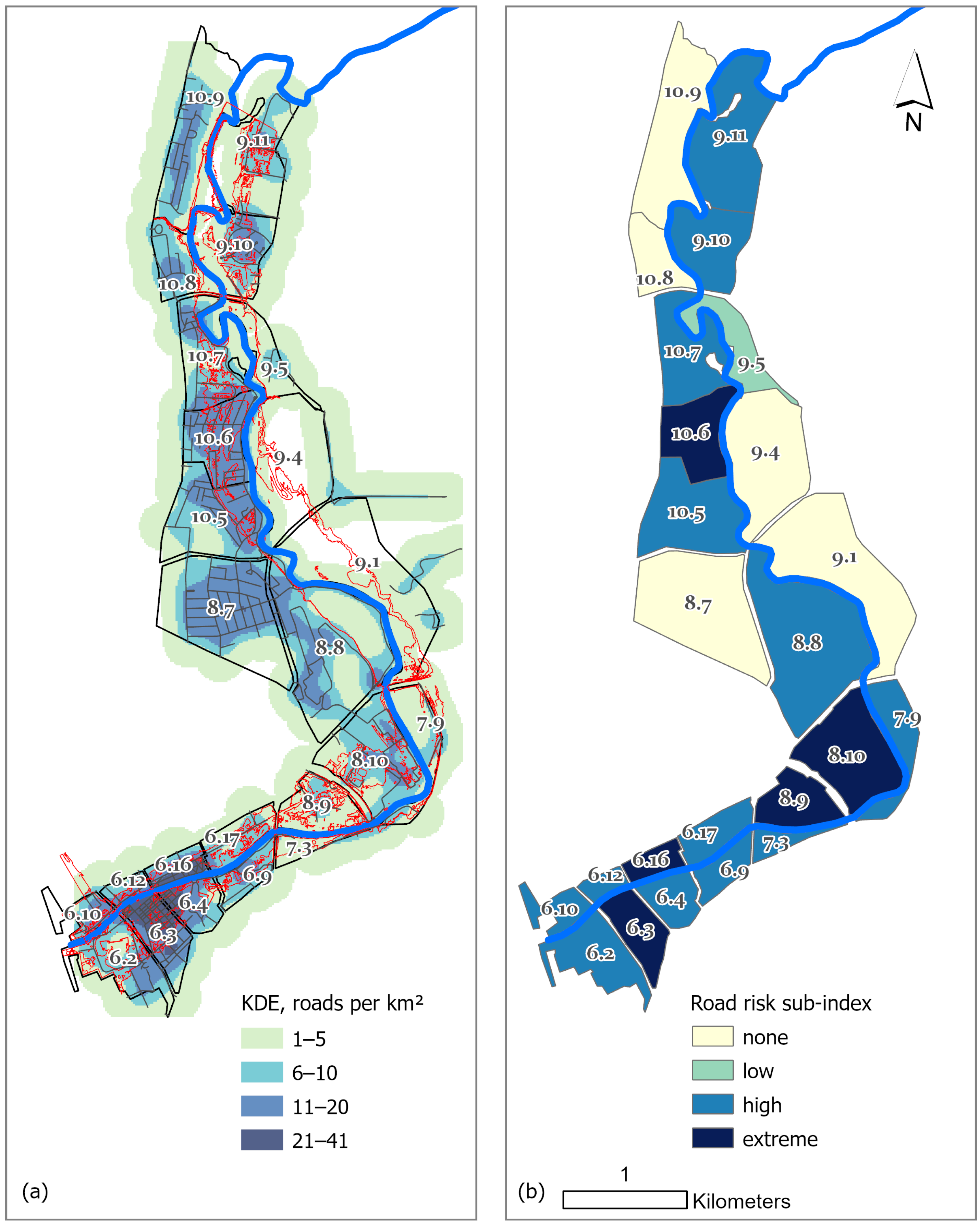
The largest flood impact magnitudes were identified in several central and northern RNs, with the highest flooded road lengths reaching up to 4.0 km (Table A2). This is also confirmed by the spatial analysis, which shows that the highest road-infrastructure concentrations (KDE) and the highest-risk zones coincide along the Danė River, especially in the central part of the city (Figure 6a). These areas should be treated as priorities when planning traffic management and flood risk reduction measures.

Based on relative road exposure, five RNs show no risk, one shows low risk, two show medium risk, four show high risk, and as many as 12 fall into the extreme exposure category (Table A2). The highest-risk group under both indicators is concentrated in several central and northern RNs, which should therefore be treated as priority areas for protection measures.

The percentage-based analysis reveals an additional aspect: in as many as nine RNs, 100% of the road infrastructure could be flooded under the extreme flood scenario. This highlights the difference between impact magnitude and relative exposure for road infrastructure, as in some RNs (e.g., RN 6.10, RN 6.12, RN 7.3, and RN 7.9), the flooded road length is small, but in percentage terms, the entire local road infrastructure may be affected. This difference shows that road infrastructure vulnerability should be assessed in a combined way.

Using the mean of the two indicator scores to calculate the road risk SI, the RNs were distributed as follows: five RNs with no risk, one with low risk, 13 with high risk, and five with extreme risk (Figure 6b). These results indicate that flooding may have a substantial impact on the city’s transport infrastructure in the context of climate change, especially where higher road concentrations coincide with flood-prone areas. SI-based risk assessment, supported by flood-exposure data, provides a stronger basis for identifying priority RNs where infrastructure resilience should be strengthened and preventive measures applied.

3.2.3. Population Risk SI

Buildings and roads located within the flood zone directly affect residents, their property, and daily mobility. Accordingly, areas with the highest building concentrations also tend to have the highest population counts. However, population flood risk depends not only on the total population in an RN but also on whether densely populated areas overlap with the flood zone. Under the extreme compound flood scenario, the flood zone expands into urbanised areas, including densely populated neighbourhoods, so flood impacts can be felt directly by residents.

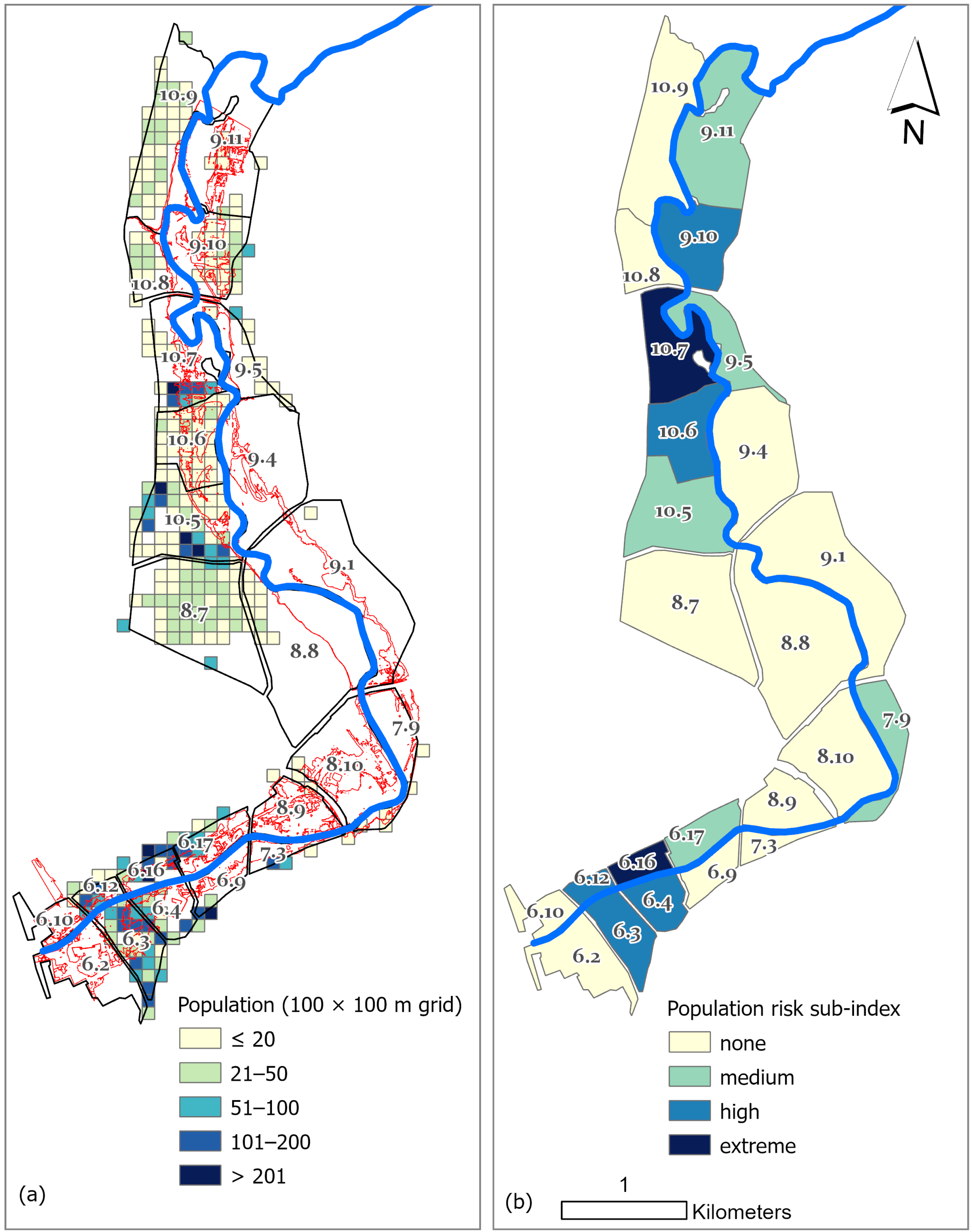
Among the analysed RNs, the highest population is concentrated in several densely populated RN. A high total population alone does not necessarily imply flood-related risk, as some densely populated RNs have no direct contact with the Danė River and therefore remain unaffected across the assessed elements. In contrast, other densely populated areas overlap with flood-prone zones, increasing socio-economic risk. Overall, population distribution is highly uneven, ranging from 8 to 11,407 residents. The highest population concentrations are spatially clustered in the central and northern parts of the city (Figure 7a; Table A3).

Based on the risk SI, while 12 RNs remain in the no-risk category at all stages, five RNs show medium risk, five show high risk, and two show extreme risk (Figure 7b). These results also highlight the locational sensitivity of population exposure, as the largest population concentrations are found in residential neighbourhoods in the Old Town and the northern part of the city, where flood impacts become more significant. This indicates that residential development, especially in currently less populated RNs, may increase both flood impact magnitude and overall vulnerability in the future if it proceeds without considering climate change scenarios and integrated risk assessment.

3.2.4. Business Entities SI

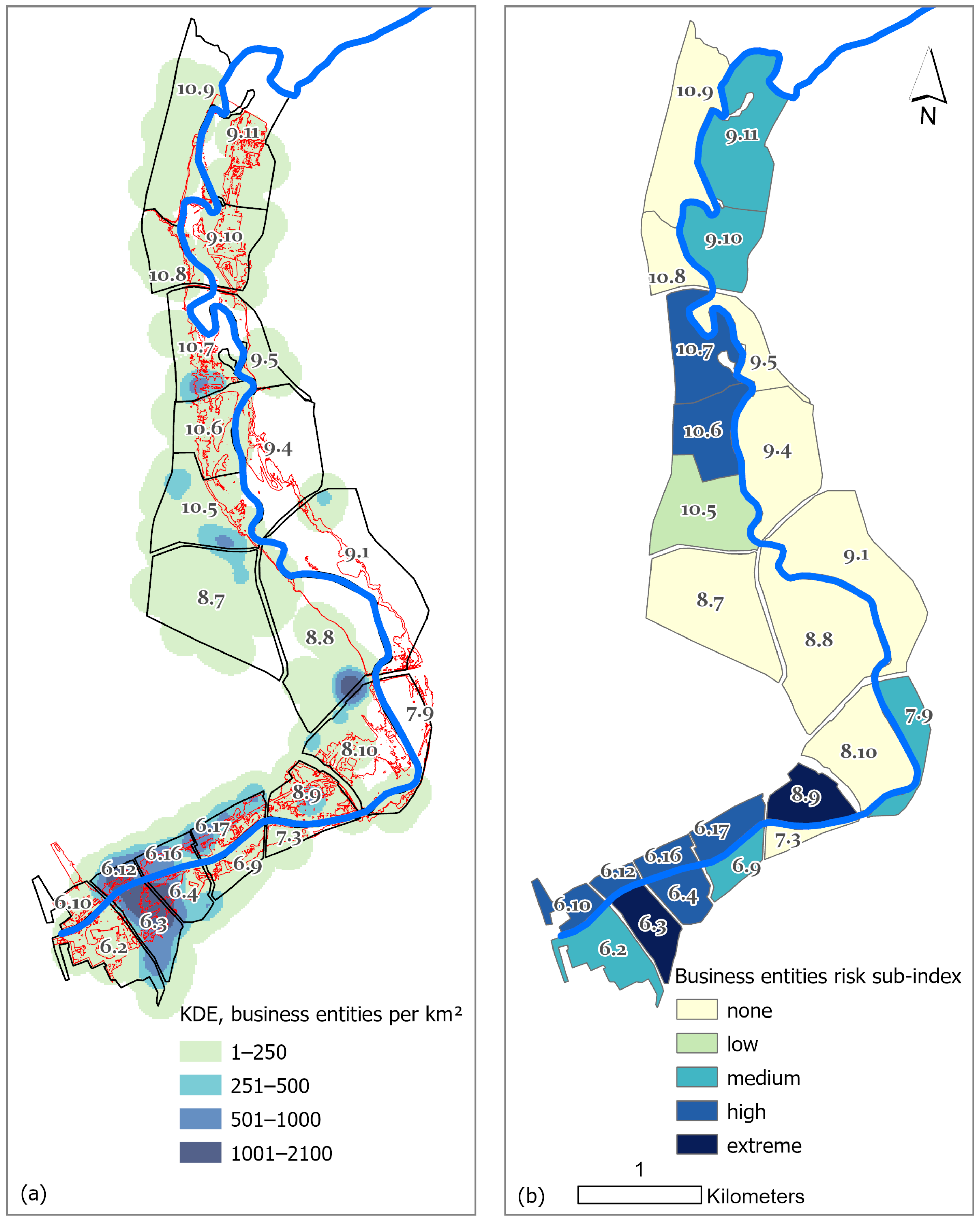
Based on impact magnitude, nine RNs show no business-entity flood risk, meaning that under the extreme flood scenario, business entities do not fall within the flood zone (Table A4). Among the remaining RNs, four were categorised as low-impact magnitude, four as medium, four as high, and three as extreme. In the extreme category, the number of flooded business entities ranges from 34 to 156, with the highest value recorded in Senamiesčio. Based on relative exposure, nine RNs also remain in the no-risk category. Among the remaining RNs, one was categorised as low, nine as medium, two as high, and three as extreme. The highest business-entity concentrations (KDE) are clustered in the central part of the city (Figure 8a).

Comparing impact magnitude and relative exposure shows that the risk category changes in some RNs because the total number of business entities differs between RNs. For example, some central RNs are categorised as extreme based on impact magnitude, but only as high based on relative exposure, because a substantial share of business entities remains outside the flood zone. Other RNs are categorised as high based on relative exposure, because more than half of the business entities are flooded. The most pronounced shifts are observed in RNs where a large share of business entities is affected. In some cases, risk remains extreme under both indicators because all business entities are flooded. In other RNs, the absolute number of flooded business entities is small, but relative exposure is extreme because most local business entities fall within the flood zone. A similar pattern is observed in some mixed-use and industrial RNs, where impact magnitude is only moderate, but relative exposure reaches extreme values because most business entities in the RN are flooded.

Based on the business entities SI (the mean of the impact magnitude and relative exposure scores), nine RNs show no risk, one is categorised as low risk, five as medium, seven as high, and two as extreme (Figure 8b). This result particularly highlights the vulnerability of Mažosios lankos (8.9), as this RN is classified as an industrial area.

3.2.5. Cultural Heritage Entities Risk SI

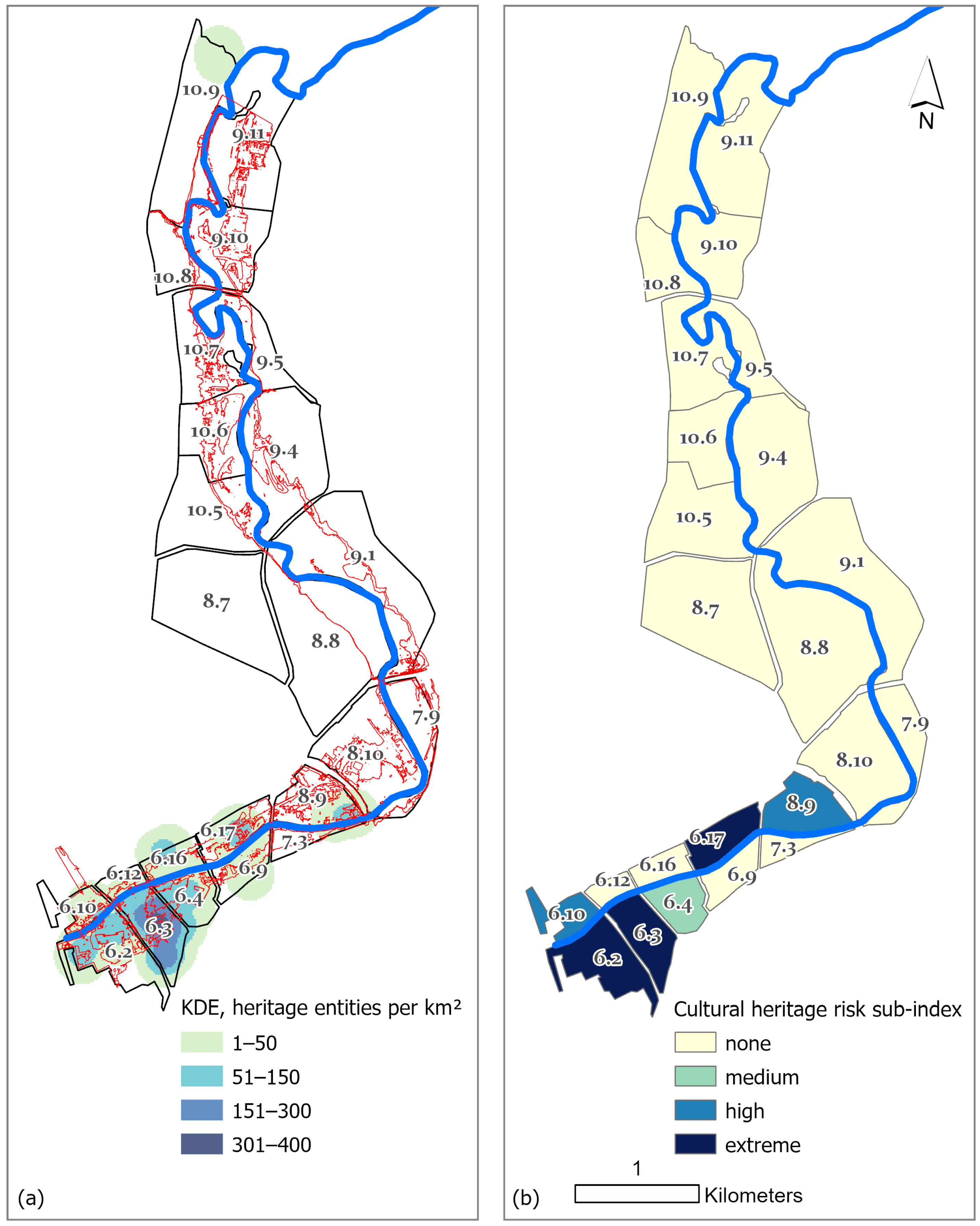
Based on impact magnitude, most RNs show no flood risk to cultural heritage objects, as these objects do not fall within the flood zone under the extreme flood scenario (Table A5). In total, 18 RNs are categorised as no risk, two as low, one as medium, one as high, and two as extreme based on impact magnitude. Based on relative exposure, 18 RNs also remain in the no-risk category. Among the remaining RNs, one is categorised as medium, two as high, and three as extreme. This shows that in some RNs, even when the number of flooded heritage objects is small, a large share of the total cultural heritage objects in the RN may be affected. The highest cultural heritage object concentrations (KDE) are clustered in the central part of the city, and the highest-risk zones coincide with areas where flooding affects a substantial share of cultural heritage objects (Figure 9a).

The comparison of impact magnitude and relative exposure reveals category shifts in some RNs, driven by differences in the total number of cultural heritage entities. For example, in some RNs, only a small number of cultural heritage entities are flooded based on impact magnitude, but this corresponds to full exposure because all cultural heritage objects in the RN are affected. In contrast, some central RNs remain high-impact areas because of the large number of flooded entities, although under relative exposure, they fall into the high category rather than the extreme category.

Based on the cultural heritage objects risk SI (the mean of the impact magnitude and relative exposure scores), the no-risk group remains dominant. Extreme risk SI values were recorded in three RNs, while high and medium risk SI values were identified in only a few additional, mostly central RNs (Figure 9b). Spatial analysis confirms that the highest concentrations of cultural heritage objects are clustered in the central part of the city, where the highest risk SI values are also observed.

3.3. CSERI-Based Socio-Economic Flood Risk Assessment

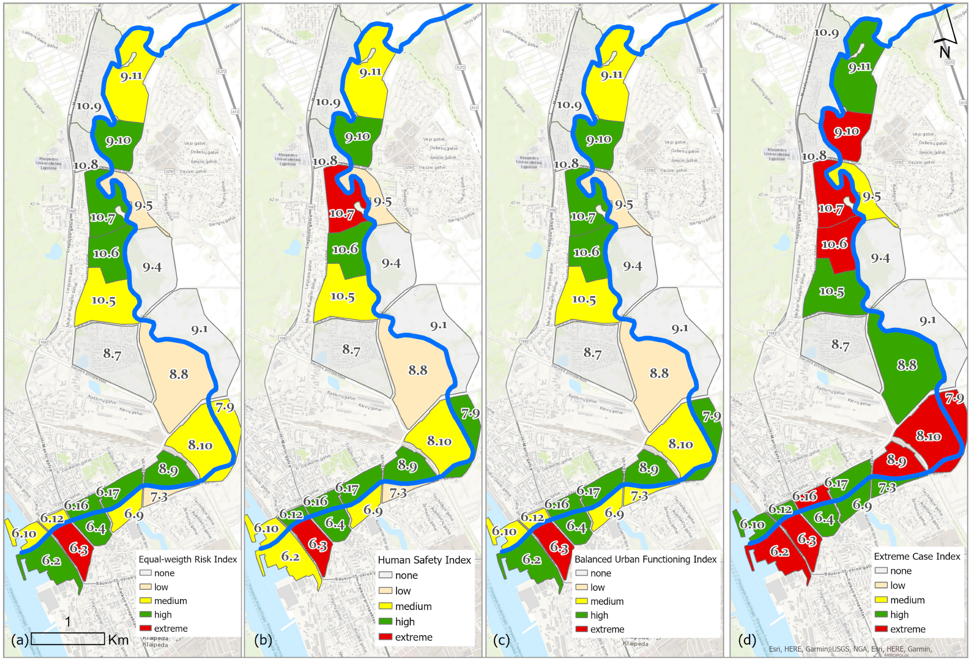
CSERI values depend strongly on the level of urbanisation in the RNs. The RNs along the Danė River differ significantly in their degree of development. Some are dominated by densely built residential areas with well-developed infrastructure and large populations, while others are characterised by more natural, less human-modified environments with open spaces. These differences lead to different levels of sensitivity to climate change and require different flood risk reduction and adaptation measures. From a sustainability perspective, the results indicate that future urban development in flood-prone areas may intensify long-term socio-economic vulnerability if it is not guided by climate-resilient planning principles. To make the results useful for different planning objectives, the composite assessment uses four indices: the equal-weight CSERI, the human safety CSERI, the balanced urban functioning CSERI, and the extreme-case index (

Table A6. Risk SI values and CSERI for RNs under four weighting scenarios.

RN Name	Risk SI Values					CSERI
	Buildings	Road Infrastructure	Population	Business Entities	Cultural Heritage	Equal Weight	Human Safety	Balanced Urban Functioning	Extreme Case
6.2 Piliavietės	2.5	3	0	2	3.5	2.2	1.8	2.1	3.5
6.3 Senamiesčio	3.5	4	3	3.5	3.5	3.5	3.4	3.5	4.0
6.4 Bastioninių įtvirtnimų	2	2.5	3	2.5	1.5	2.3	2.5	2.4	3.0
6.9 Pelenyno	2.5	3	0	2	0	1.5	1.4	1.6	3.0
6.10 Šiaurės rago	2.5	2.5	0	2.5	3.5	2.0	1.6	1.9	2.5
6.12 Rotušės	2	2.5	2.5	2.5	0	1.9	2.2	2.0	2.5
6.16 Senosios elektrinės I	2	3.5	3.5	3	0	2.4	2.8	2.6	3.5
6.17 Senosios elektrinės II	3	3	2	2.5	0	2.8	2.6	2.8	3.0
7.3 Joniškės III	2.5	2.5	0	0	0	1.0	1.0	1.1	2.5
7.9 Upės uosto	3.5	2.5	2	1.5	0	1.9	2.1	2.1	3.5
8.9 Mažosios lankos	4	4	0	4	3	3.0	2.5	2.9	4.0
8.10 Luizės dvaro	3	4	0	0	0	1.4	1.4	1.6	4.0
8.7 Karališkosios giraitės	0	0	0	0	0	0.0	0.0	0.0	0.0
8.8 Paupių pievos	0	2.5	0	0	0	0.5	0.5	0.6	2.5
9.1 Daugulių	0	0	0	0	0	0.0	0.0	0.0	0.0
9.4 Luizės ąžuolo I	0	0	0	0	0	0.0	0.0	0.0	0.0
9.5 Luizės ąžuolo II	1	1	1.5	0	0	0.7	0.9	0.8	1.5
9.10 Dvaro slėnio I	3.5	2.5	2.5	2	0	2.1	2.4	2.3	3.5
9.11 Dvaro slėnio II	2.5	2.5	1.5	1.5	0	1.6	1.8	1.7	2.5
10.5 Miestiečių laukų I	2.5	2.5	1.5	1	0	1.5	1.7	1.7	2.5
10.6 Miestiečių laukų II	3.5	4	3	3	0	2.7	3.0	2.9	4.0
10.7 Miestiečių laukų III	3	3	4	3	0	2.6	3.1	2.8	4.0
10.8 Didžiojo Tauralaukio I	0	0	0	0	0	0.0	0.0	0.0	0.0
10.9 Didžiojo Tauralaukio II	0	0	0	0	0	0.0	0.0	0.0	0.0

, Figure 10). It is important to note that the risk SI values shown in the tables and used for plotting were rounded. However, unrounded values were used to calculate the composite indices, so the final indices reflect the risk distribution more consistently.

The equal-weight CSERI combines all risk SIs using equal weights. The extreme and high values were identified in five RNs, indicating that these areas are likely to experience the strongest composite socio-economic flood impacts. Medium values were recorded in three RNs, while lower non-zero values were found in several additional RNs where the component risks do not accumulate at the same time. The spatial pattern shows that the highest values are concentrated in the central part of the city and along the more intensively urbanised banks of the Danė River (Figure 10a). RNs with a zero index value (0.0) indicate that no vulnerability was identified there under the modelled extreme flood scenario and the selected socio-economic components. Therefore, priority risk-reduction and adaptation measures should be focused on areas with the highest index values. However, if these areas are developed more intensively in the future, development should follow climate-resilient planning criteria and flood prevention measures, including building restrictions, stormwater management, and the integration of green and engineering solutions, to maintain safety under changing climate conditions. RNs with a consistent value of 0.0 across all assessed composite indices are not discussed further. The following analysis focuses on areas with higher index values that require priority adaptation and risk-reduction measures.

The human safety CSERI highlights areas where flood risk is most relevant to residents. Excluding 0.0 values, the index ranges from 0.5 to 3.4 (Figure 10b). The extreme and high values were recorded in four RNs, indicating the highest likelihood of social impacts during an extreme flood in these areas. This is also confirmed by the spatial distribution of the index, which shows that the highest human-safety-related risk is concentrated in densely urbanised flood-prone areas in the central and northern parts of the city.

The balanced urban functioning CSERI reflects the city’s ability to maintain balanced functioning during floods. In this index, the highest weights are assigned to infrastructure and population (0.25 each) because of their role in mobility and access to services, while buildings (0.20), business entities (0.15), and cultural heritage objects (0.15) represent material, economic, and cultural losses. Excluding 0.0 values, the index ranges from 0.6 to 3.5 and highlights areas where the greatest disruption of urban functioning is expected during floods (Figure 10c). The highest and high values were recorded in six RNs, while notable values are also observed in a small number of RNs. Overall, the spatial pattern indicates that the strongest disruption of urban functioning is concentrated in the central part of the city and in several intensively urbanised flood-prone areas along the Danė River.

In the extreme-case index, risk is defined by the highest value among the risk SIs. Excluding 0.0 values, the index ranges from 1.5 to 4.0 and makes it possible to identify areas where at least one component reaches a critical level even when the overall risk level is not high (Figure 10d). The highest value (4.0) was recorded in five RNs, indicating that in these areas, at least one vulnerability component (buildings, infrastructure, population, business entities, or cultural heritage objects) is strongly affected during an extreme flood. High values (3.5) were identified in four additional RNs, while values of 3.0 were observed in three RNs. This suggests that risk-management measures in these areas should be targeted to the specific dominant component that reaches the maximum value. Lower extreme-case index values indicate a weaker influence of any single component.

Overall, the distribution of all four composite indices shows a consistent relationship between flood risk and the urbanised areas along the Danė River. In all cases, higher values are concentrated in the central part of the city and in intensively urbanised stretches, where denser building patterns, infrastructure, population concentration, and economic activity overlap. The equal-weight CSERI highlights overall vulnerability and clearly identifies the main risk hotspots in the central part of the city. The human safety CSERI places greater emphasis on areas where floods could have the strongest social impact on residents, again highlighting the central part of the city near the Klaipėda Strait and intensively built RNs in the northern part of the city. The balanced urban functioning CSERI emphasises areas where flooding could disrupt the continuity of transport, engineering networks, and economic functions, thereby highlighting functionally important urban links and activity concentration zones that overlap with the pattern of the human safety CSERI. In contrast, the extreme-case index identifies areas where risk-management measures should be targeted to the dominant vulnerability component. The results confirm that priority adaptation and risk-reduction measures should be focused on central and functionally important Danė riverside areas, while in lower-value areas, the key priority is to ensure that any future development follows climate-resilient planning principles.

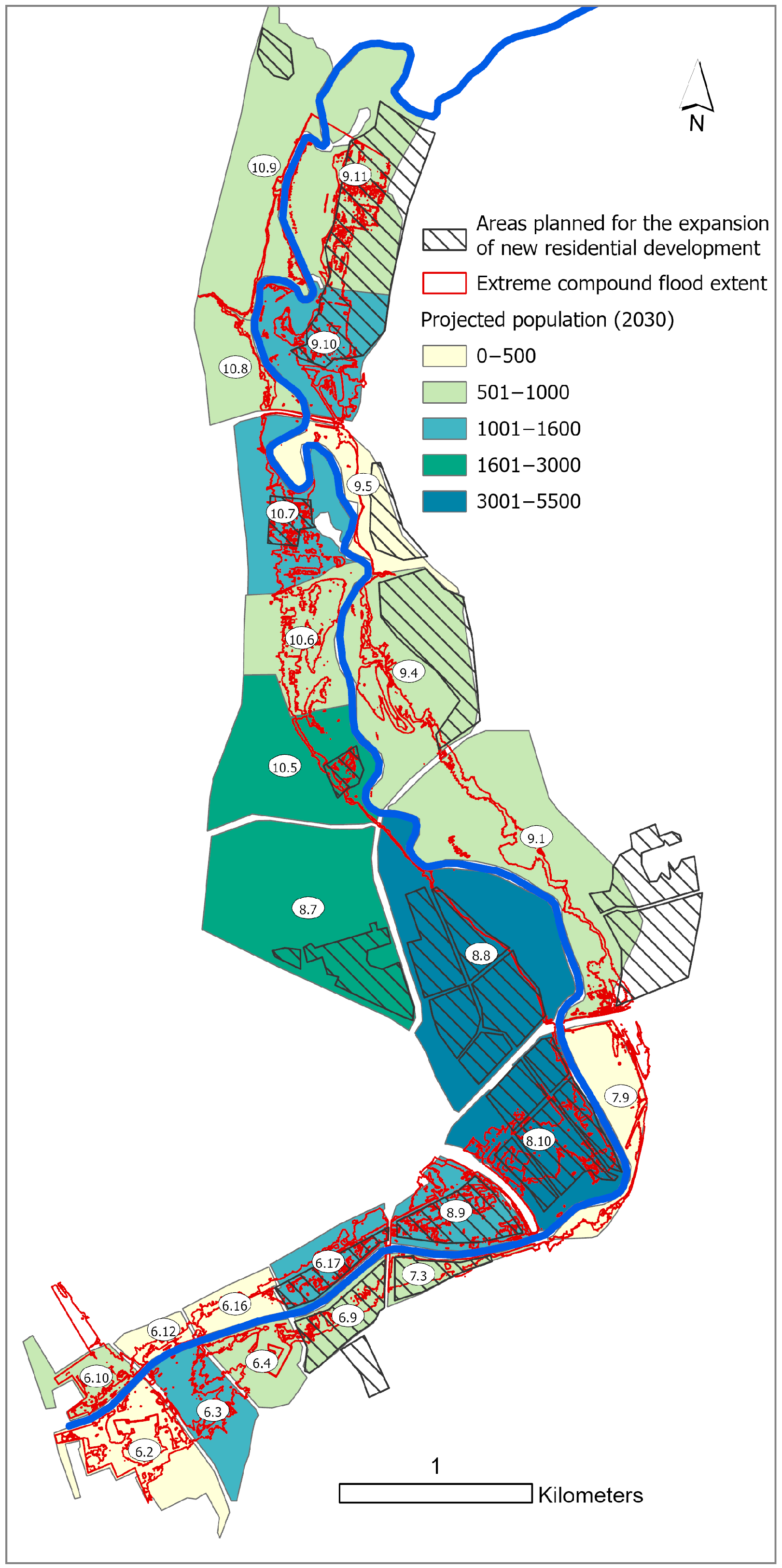
In the context of long-term urban development, the 2030 population forecast from the Klaipėda City Master Plan was used to characterise potential future exposure in the analysed RNs. These data are relevant because the projected population size directly affects the potential number of people exposed during flooding. The total population projected for these RNs is about 32,000. The highest projected population is concentrated in several northern and peripheral RNs, where it may reach up to 5500 in one RN and up to 3000 in two additional RNs (Figure 11). In several other RNs, the projected population ranges up to 1200, while in others, it remains below 700.

The Klaipėda City Master Plan also states that, in order to reduce migration of city residents to suburban areas, specific territories will be designated for residential development within the city. Intensive planned development overlapping with the extreme compound flood scenario is projected in several central, northern, and eastern RNs. If these Master Plan provisions are implemented, socio-economic losses are likely to increase in the future, as a larger share of these areas will fall within the flood-risk zone. The selection of these territories as development zones also introduces additional risks according to the sub-indices and composite indices calculated in this study. The results show that in these RNs, multiple risk-enhancing components often coincide.

4. Discussion

Areas that are currently flooded approximately once in 100 years may be flooded significantly more frequently under climate change scenarios. This indicates that under climate change conditions, not only the flood extent but also the frequency of flood occurrence is changing. The highest risk is concentrated in urbanised areas located in terrain depressions. It is also important that some areas that are currently not officially included in the risk zone may become vulnerable in the long term when climate change effects are taken into account. This trend is also confirmed by the risk SI results, which reveal the sensitivity of RNs across the analysed components. Such a mismatch may lead to inappropriate spatial planning decisions in the near future and, consequently, to greater socio-economic losses over time. Vulnerability is further increased by the concentration of flooded buildings, exposed residents, and projected population growth in RNs, together with dense infrastructure, business entities, and cultural heritage objects that may be affected by extreme hydrometeorological events. Including these areas in risk zones and applying risk reduction measures would help reduce future damage, protect residents, and lower long-term infrastructure recovery costs. In this context, the composite risk index provides a more comprehensive and integrated basis for identifying areas where risk is driven by the cumulative vulnerability of multiple components.

The proposed CSERI in this study enables a spatial comparison of the socio-economic risk of residential neighbourhoods under an extreme compound flood scenario, based on the distribution of exposed elements and the potential extent of impact. However, some factors that may influence the differentiation of flood consequences were not explicitly incorporated into the current index structure. These include road hierarchy, drainage system capacity, and more detailed characteristics of social sensitivity, such as age structure, disability, income level, or other indicators related to social vulnerability. Therefore, the results should be interpreted as a comparative spatial representation of neighbourhood-level socio-economic risk under the selected scenario. Future research could further develop this approach by integrating more detailed infrastructure data, social indicators, and questionnaire-based analysis of residents’ experiences.

Accordingly, the present assessment should be interpreted as a scenario-based comparative analysis of neighbourhood-level socio-economic risk under the selected scenario. Validation against observed socio-economic damage data at the residential neighbourhood level would provide an important next step in further developing the approach.

Accordingly, it is important to consider that the most densely populated areas either fall within flood-risk zones or are located adjacent to them. Therefore, any planned residential development in these areas should be implemented together with climate change adaptation measures. In urban planning, alongside decisions related to residential expansion and residents’ needs, flood-risk reduction solutions should also be integrated, such as stormwater management, elevated engineering networks, and adjustments to urban design in low-lying areas. Planning decisions should be prioritised according to the RN-based index results. This is particularly important for creating safe, resilient, and long-term residential areas, helping to avoid future climate-related losses and reduce potential impacts.

Existing built-up areas need to be adapted to reduce their vulnerability. However, intensifying residential development in these areas would make future adaptation more challenging and more expensive. Sea-level rise and the associated flood hazard may cause significant economic damage in these areas. The importance of adaptation to climate change is recognised globally, yet in practice, preparedness remains insufficient even for current extreme events. Areas where climate change impacts are already evident should be systematically reconfigured to reduce both economic and social vulnerability. The new EU Strategy on Adaptation to Climate Change [57] emphasises that climate change factors and related risks must be assessed systematically in urban development planning. Therefore, new construction near water bodies should be restricted and allowed only where clear risk-reduction measures are in place.

Given the impacts of climate change and the increasing frequency of extreme hydrometeorological events, one possible adaptation measure is the construction of artificial embankments, especially in high-risk RNs. However, to ensure that such measures are appropriate, technically justified, and cost-effective, detailed hydrodynamic modelling and local geotechnical investigations are required first. These studies should include an assessment of the current bank condition, an evaluation of the hydraulic effectiveness of the planned embankments, and an analysis of potential impacts on adjacent areas. Properly implemented bank reinforcement, together with river-flow regulation measures, can reduce slope erosion, protect urban infrastructure and residents, and significantly reduce potential socio-economic damage in the context of climate change and anthropogenic pressure. Such engineering measures are most appropriate in areas where the composite index indicates high risk.

In addition to the main structural measures, it is important to integrate green infrastructure, particularly by increasing tree cover and vegetation in low-lying areas and restoring natural surface-runoff infiltration and retention systems. Preparedness measures should include strengthening flood forecasting and modernising resident warning systems. In urbanised areas, comprehensive planning measures are also essential, such as maintaining non-buildable buffer zones, ensuring adequate stormwater collection, and designing new neighbourhoods with explicit consideration of flood-prone areas.

The results of this study show that flood risk is shaped by the spatial overlap of multiple components, including buildings, infrastructure, population, business entities, and cultural heritage objects. Therefore, adaptation planning should not rely on a single indicator but should account for all analysed components and their different roles in urban functioning and vulnerability. In particular, the population component is critical because residents may face both tangible and intangible impacts during floods. Tangible impacts include direct damage to housing, property, and access to essential infrastructure, while intangible impacts may include stress, anxiety, and longer-term psychosocial strain. In this context, the use of risk SIs and the composite index provides a practical basis for identifying priority areas and selecting measures according to the dominant risk components, helping to ensure that adaptation responses are targeted, consistent, and systematic.

5. Conclusions

In Klaipėda City, compound flood risk is driven by the interaction between water levels in the Klaipėda Strait and Danė River discharge. Marine storm surges raise the Danė water level in the urban area, and when additional hydrometeorological factors contribute, compound floods can develop and reach extreme levels.

Risk SIs were calculated for the selected urban elements (buildings, roads, population, business entities, and cultural heritage objects), enabling assessment of the contribution of individual components to flood risk across RNs and supporting more targeted risk-reduction measures. Combined with KDE analysis, the SI results helped identify priority areas and the dominant risk factors within them.

The developed CSERI indices were calculated by combining the five component-specific risk SIs (buildings, roads, population, business entities, and cultural heritage objects) under different weighting schemes. This approach makes it possible to compare urban areas comprehensively across different dimensions of vulnerability and to define priorities for decision-making. The equal-weight CSERI reflects overall vulnerability, the human safety CSERI highlights areas with the greatest potential social impact on residents, the balanced urban functioning CSERI emphasises the risk of disruption to mobility and continuity of urban functions, and the extreme-case index identifies areas where risk is determined by the critical impact of a single dominant component. The results show that the highest-risk zones are concentrated in the central part of the city and in several RNs in the northern part of the city, where multiple exposed elements are concentrated and overlap with the flood zone.

Beyond hazard assessment, the proposed index contributes to sustainability by supporting more balanced urban development, reducing future exposure, and promoting climate-resilient planning in coastal cities.

Integrated assessments of compound flood risk and socio-economic impacts should be systematically integrated into urban planning and development decisions. They help identify areas with the highest exposure and potential losses and, accordingly, guide infrastructure protection, land-use planning, and preventive measures before new development is implemented. Such measures are essential for climate change adaptation and for reducing or avoiding potential socio-economic losses.

The proposed CSERI framework may also be applied in other coastal cities as a comparative tool for identifying socio-economic risk under extreme flood conditions. Moreover, the methodology is not limited to residential neighbourhoods and may also be applied using regular grid-based units, where appropriate data are available, enabling more flexible comparison of flood-exposed urban areas across different spatial scales.

References

1. Dangendorf, S.; Sun, Q.; Gamage, P.M.M.; Wahl, T.; Marcos, M.; Marzeion, B.; Slangen, A.; Mitrovica, J. Human-driven sea-level rise has tripled the frequency of coastal sea-level extremes since 1900. Res. Sq. 2025. Preprint. [Google Scholar] [CrossRef]
2. Eelsalu, M.; Soomere, T.; Parnell, K.; Viška, M. Attribution of alterations in coastal processes in the southern and eastern Baltic Sea to climate change-driven modifications of coastal drivers. Oceanologia 2025, 67, 1–38. [Google Scholar] [CrossRef]
3. Reckermann, M.; Omstedt, A.; Soomere, T.; Aigars, J.; Akhtar, N.; Bełdowska, M.; Bełdowski, J.; Cronin, T.; Czub, M.; Eero, M.; et al. Human impacts and their interactions in the Baltic Sea region. Earth Syst. Dyn. 2022, 13, 1–80. [Google Scholar] [CrossRef]
4. Kudryavtseva, N.; Soomere, T.; Männikus, R. Non-stationary analysis of water level extremes in Latvian waters, Baltic Sea, during 1961–2018. Nat. Hazards Earth Syst. Sci. 2021, 21, 1–23. [Google Scholar] [CrossRef]
5. Zalewska, T.; Kowalska, B.; Krzysztofik, K.; Sapiega, P. Changes in Sea Level, Storm and Wave Conditions, and Ice Cover—Over 70 Years of Observation in the Southern Baltic Sea. Water 2025, 17, 680. [Google Scholar] [CrossRef]
6. Dailidienė, I.; Stankevičius, A.; Tilickis, B. Peculiarities of the long-term water level fluctuations in the south-eastern part of the Baltic Sea and the Curonian Lagoon. Geod. Cartogr. 2004, 30, 58–64. [Google Scholar]
7. Dailidienė, I.; Davulienė, L.; Tilickis, B.; Stankevičius, A.; Myrberg, K. Sea level variability at the Lithuanian coast of the Baltic Sea. Boreal Environ. Res. 2006, 11, 109–121. [Google Scholar]
8. Dailidienė, I.; Baudler, H.; Chubarenko, B.; Navrotskaya, S. Long term water level and surface temperature changes in the lagoons of the southern and eastern Baltic. Oceanologia 2011, 53, 293–308. [Google Scholar] [CrossRef]
9. Green, J.; Haigh, I.D.; Quinn, N.; Neal, J.; Wahl, T.; Wood, M.; Eilander, D.; de Ruiter, M.; Ward, P.; Camus, P. A comprehensive review of compound flooding literature with a focus on coastal and estuarine regions. Nat. Hazards Earth Syst. Sci. 2025, 25, 747–816. [Google Scholar] [CrossRef]
10. Xu, K.; Wang, C.; Bin, L. Compound flood models in coastal areas: A review of methods and uncertainty analysis. Nat. Hazards 2023, 116, 469–496. [Google Scholar] [CrossRef]
11. Sebastian, A. Compound flooding. In Coastal Flood Risk Reduction: The Netherlands and the U.S. Upper Texas Coast; Brody, S., Lee, Y., Kothuis, B.B., Eds.; Elsevier: Amsterdam, The Netherlands, 2022; pp. 77–88. [Google Scholar] [CrossRef]
12. Dubois, K.; Nilsson, E.; Larsen, M.A.D.; Drews, M.; Hieronymus, M.; Karami, M.P.; Rutgersson, A. Exploring storm tides projections and their return levels around the Baltic Sea using a machine learning approach. Tellus A Dyn. Meteorol. Oceanogr. 2025, 77, 79–97. [Google Scholar] [CrossRef]
13. Viigand, K.; Eelsalu, M.; Soomere, T. Quantifying exposedness of the eastern Baltic Sea shores with respect to extremely high and low water levels. Estuar. Coast. Shelf Sci. 2025, 319, 109267. [Google Scholar] [CrossRef]
14. Cabana, D.; Celliers, L. Climate information to action: Challenges for Baltic beach management. Ocean Coast. Manag. 2025, 269, 107777. [Google Scholar] [CrossRef]
15. Higuera Roa, O.; Bachmann, M.; Mechler, R.; Šakić Trogrlić, R.; Reimann, L.; Mazzoleni, M.; Aerts, J.C.J.H.; Buskop, F.E.; Pirani, A.; Mysiak, J. Challenges and opportunities in climate risk assessment: Future directions for assessing complex climate risks. Environ. Res. Lett. 2025, 20, 053003. [Google Scholar] [CrossRef]
16. Endendijk, T.; Botzen, W.J.W.; de Moel, H.; Aerts, J.C.J.H.; Slager, K.; Kok, M. Flood vulnerability models and household flood damage mitigation measures: An econometric analysis of survey data. Water Resour. Res. 2023, 59, e2022WR034192. [Google Scholar] [CrossRef]
17. Armenakis, C.; Du, E.X.; Natesan, S.; Persad, R.A.; Zhang, Y. Flood risk assessment in urban areas based on spatial analytics and social factors. Geosciences 2017, 7, 123. [Google Scholar] [CrossRef]
18. Bidadian, B.; Strager, M.P.; Ghadimi, H.; Sharma, M. Flood exposure, vulnerability, and risk distribution in urban areas: Application of geospatial data analytics and index development. GeoHazards 2024, 5, 833–852. [Google Scholar] [CrossRef]
19. Birkmann, J. Risk and vulnerability indicators at different scales: Applicability, usefulness and policy implications. Environ. Hazards 2007, 7, 20–31. [Google Scholar] [CrossRef]
20. Balica, S.F.; Wright, N.G.; Van der Meulen, F. A flood vulnerability index for coastal cities and its use in assessing climate change impacts. Nat. Hazards 2012, 64, 73–105. [Google Scholar] [CrossRef]
21. Yılmaz, M.; Alemdar, K.D. An integrated methodology for flood risk assessment of road networks: A case study of Ordu, Türkiye. Model. Earth Syst. Environ. 2025, 11, 447. [Google Scholar] [CrossRef]
22. UNISDR. UNISDR Terminology on Disaster Risk Reduction; United Nations Office for Disaster Risk Reduction (UNISDR): Geneva, Switzerland, 2009; Available online: https://www.preventionweb.net/files/7817_UNISDRTerminologyEnglish.pdf (accessed on 4 February 2026).
23. Arrighi, C.; Ballio, F.; Simonelli, T. A GIS-based flood damage index for cultural heritage. Int. J. Disaster Risk Reduct. 2023, 90, 103654. [Google Scholar] [CrossRef]
24. Garrote, J.; Díez-Herrero, A.; Escudero, C.; García, I. A framework proposal for regional-scale flood-risk assessment of cultural heritage sites and application to the Castile and León Region (Central Spain). Water 2020, 12, 329. [Google Scholar] [CrossRef]
25. Kim, J.; Sung, H.H. Assessing flood risk of heritage sites in an urban area: Impact of locational characteristics and historical context. Sustainability 2024, 16, 10473. [Google Scholar] [CrossRef]
26. Mah, J.C.; Penwarden, J.L.; Pott, H.; Theou, O.; Andrew, M.K. Social vulnerability indices: A scoping review. BMC Public Health 2023, 23, 1253. [Google Scholar] [CrossRef]
27. Samsuddin, A.; Kaman, Z.K.; Mat Husin, N. Socio-economic assessment on flood risk impact: A methodological review toward environmental sustainability. IOP Conf. Ser. Earth Environ. Sci. 2021, 943, 012010. [Google Scholar] [CrossRef]
28. Gallè, F.; Valeriani, F.; De Giorgi, A.; Grassi, F.; Mazzeo, E.; Napoli, C.; Protano, C. Assessing the presence of eco-anxiety in the general population: A systematic review, meta-analysis and meta-regression. Healthcare 2025, 13, 2716. [Google Scholar] [CrossRef]
29. Walinski, A.; Sander, J.; Gerlinger, G.; Clemens, V.; Meyer-Lindenberg, A.; Heinz, A. The effects of climate change on mental health. Dtsch. Aerztebl. Int. 2023, 120, 117–124. [Google Scholar] [CrossRef]
30. Pihkala, P. Toward a taxonomy of climate emotions. Front. Clim. 2022, 3, 738154. [Google Scholar] [CrossRef]
31. van Heel, B.F.; van den Born, R.J.G. Studying residents’ flood risk perceptions and sense of place to inform public participation in a Dutch river restoration project. J. Integr. Environ. Sci. 2020, 17, 35–55. [Google Scholar] [CrossRef]
32. Osberghaus, D. The determinants of private flood mitigation measures in Germany—Evidence from a nationwide survey. Ecol. Econ. 2015, 110, 36–50. [Google Scholar] [CrossRef]
33. Munro, A.; Kovats, R.S.; Rubin, G.J.; Waite, T.D.; Bone, A.; Armstrong, B.; English National Study of Flooding and Health Study Group. Effect of evacuation and displacement on the association between flooding and mental health outcomes: A cross-sectional analysis of UK survey data. Lancet Planet. Health 2017, 1, e134–e141. [Google Scholar] [CrossRef]
34. Houston, D.; Ball, T.; Werritty, A.; Black, A.R. Social influences on flood preparedness and mitigation measures adopted by people living with flood risk. Water 2021, 13, 2972. [Google Scholar] [CrossRef]
35. Endendijk, T.; Botzen, W.J.W.; de Moel, H.; Aerts, J.C.J.H.; Duijndam, S.J.; Slager, K.; Kolen, B.; Kok, M. Experience from the 2021 floods in the Netherlands: Household survey results on impacts and responses. J. Coast. Riverine Flood Risk 2023, 2, 0009. [Google Scholar] [CrossRef]
36. Čepienė, E.; Dailidytė, L.; Stonevičius, E.; Dailidienė, I. Sea level rise impact on compound coastal river flood risk in Klaipėda city (Baltic Coast, Lithuania). Water 2022, 14, 414. [Google Scholar] [CrossRef]
37. Gailiušis, B.; Jablonskis, J.; Kovalenkovienė, M. Lietuvos Upės: Hidrografija ir Nuotėkis [Lithuanian Rivers: Hydrography and Runoff]; Lietuvos Energetikos Institutas: Kaunas, Lithuania, 2001. [Google Scholar]
38. Bučienė, A.; Vasiliauskienė, E.; Bučas, S.; Karmazienė, D.; Nekrošienė, R. Retrospective ties of Lake Kalotė with the Baltic Sea and the Akmena-Danė River, western Lithuania. Baltica 2023, 36, 51–62. [Google Scholar] [CrossRef]
39. Klaipėdos Miesto Savivaldybės Administracija. Danės Upės Valymo, Gilinimo Ir Tvarkymo Darbų Klaipėdos Miesto Savivaldybės Teritorijoje Poveikio Aplinkai Vertinimo Atrankos Informacija; Screening Information for the Environmental Impact Assessment of Cleaning, Dredging and Management Works of the Danė River in the Territory of Klaipėda City Municipality; Klaipėdos Miesto Savivaldybės Administracija: Klaipėda, Lithuania, 2021; Available online: https://www.klaipeda.lt/data/public/uploads/2023/03/danes-upes-valymo-gilinimo-ir-tvarkymo-darbu-klaipedos-miesto-savivaldybes-teritorijoje-poveikio-aplinkai-vertinimo-atrankos-informacija.pdf (accessed on 15 January 2026).
40. Langas, V.; Gasiūnaitė, Z.R. Akmenos–Danės Upės Baseino Paviršinių Vandens Telkinių Taršos Mažinimo Priemonių Programa; Programme of Measures to Reduce Pollution of Surface Water Bodies in the Akmena–Danė River Basin, Report; Klaipėdos Universiteto Leidykla: Klaipėda, Lithuania, 2013. [Google Scholar]
41. Intergovernmental Panel on Climate Change (IPCC). The Concept of Risk in the IPCC Sixth Assessment Report; IPCC: Geneva, Switzerland, 2021; Available online: https://www.ipcc.ch/site/assets/uploads/2021/01/The-concept-of-risk-in-the-IPCC-Sixth-Assessment-Report.pdf (accessed on 24 March 2026).
42. United Nations Office for Disaster Risk Reduction (UNDRR). Disaster Risk Reduction Terminology. Available online: https://www.undrr.org/drr-glossary/terminology (accessed on 24 March 2026).
43. Pregnolato, M.; Ford, A.; Wilkinson, S.M.; Dawson, R.J. The impact of flooding on road transport: A depth-disruption function. Transp. Res. Part D Transp. Environ. 2017, 55, 67–81. [Google Scholar] [CrossRef]
44. Arrighi, C.; Pregnolato, M.; Dawson, R.J.; Castelli, F. Preparedness against mobility disruption by floods. Sci. Total Environ. 2019, 654, 1010–1022. [Google Scholar] [CrossRef]
45. Wang, Y.; Li, C.; Hu, Y.; Lv, J.; Liu, M.; Xiong, Z.; Wang, Y. Evaluation of urban flooding and potential exposure risk in central and southern Liaoning urban agglomeration, China. Ecol. Indic. 2023, 154, 110845. [Google Scholar] [CrossRef]
46. Fujiki, K.; Finance, O.; Hirtzel, J.; Enaux, C. Flooding and inequality: A multilevel analysis of exposure to floods and poverty in French cities. Appl. Geogr. 2024, 164, 103193. [Google Scholar] [CrossRef]
47. Sadeghi, N. Continuity of small businesses when facing increased flood risk due to global climate change impacts: A systematic literature review. Int. J. Disaster Risk Reduct. 2022, 82, 103316. [Google Scholar] [CrossRef]
48. Salazar, L.G.F.; Figueiredo, R.; Romão, X. Flood vulnerability assessment of built cultural heritage: Literature review and identification of indicators. Int. J. Disaster Risk Reduct. 2024, 111, 104666. [Google Scholar] [CrossRef]
49. Valstybės Duomenų Agentūra. Verslo Subjektai [Business Entities]. Available online: https://atviri-duomenys.stat.gov.lt/pages/veikiantys-ukio-subjektai-ir-vietos-vienetai (accessed on 17 December 2025).
50. Valstybės Duomenų Agentūra. Kultūros Paveldo Objektai [Cultural Heritage Objects]. Available online: https://atviri-duomenys.stat.gov.lt/datasets/261550584528420bba986ba1febb3f02_0/explore (accessed on 17 December 2025).
51. Valstybės Duomenų Agentūra. Gyventojų Ir Būstų Surašymo Duomenys 2021 m. [2021 Population and Housing Census Data]. Available online: https://atviri-duomenys.stat.gov.lt/datasets/7431d9532fd1439c9fb54177fbd09edb_0/explore (accessed on 17 December 2025).
52. Botev, Z.I.; Grotowski, J.F.; Kroese, D.P. Kernel density estimation via diffusion. Ann. Statist. 2010, 38, 2916–2957. [Google Scholar] [CrossRef]
53. Favretto, A. Urban Heat Island analysis with Remote Sensing and GIS methods: An application in the Trieste area (North-East of Italy). Boll. Soc. Geogr. Ital. 2018, 1, 215–229. [Google Scholar] [CrossRef]
54. Brandão, F.J.S.; Correia, R.M.; Paio, A. Measuring urban renewal: A dual kernel density estimation to assess the intensity of building renovation—Case study in Lisbon. Urban Sci. 2018, 2, 91. [Google Scholar] [CrossRef]
55. Klaipėdos Miesto Savivaldybės Administracija. Klaipėdos Miesto Savivaldybės Bendrasis Planas. Sprendiniai. Aiškinamasis Raštas; [Klaipėda City Municipality Master Plan. Solutions. Explanatory Report]; Klaipėdos Miesto Savivaldybės Administracija: Klaipėda, Lithuania, 2021; Available online: https://www.klaipeda.lt/data/public/uploads/2021/03/klaipedos-bp-aiskinamasis-rastas-2021-03-09.pdf (accessed on 5 May 2025).
56. Lehmann, A.; Getzlaff, K.; Harlaß, J. Detailed assessment of climate variability in the Baltic Sea area for the period 1958 to 2009. Clim. Res. 2011, 46, 185–196. [Google Scholar] [CrossRef]
57. European Commission. Forging a Climate-Resilient Europe—The New EU Strategy on Adaptation to Climate Change; [Kuriame atsparią klimatui Europą—naujoji ES prisitaikymo prie klimato kaitos strategija]; European Commission: Brussels, Belgium, 2021; Available online: https://eur-lex.europa.eu/legal-content/EN/TXT/PDF/?from=EN&uri=CELEX:52021DC0082 (accessed on 5 May 2025).
Figure 1. The study area: Dange River: from the Headwaters near Salantai to the Klaipėda Strait (a); location of the study area in the southeastern (SE) Baltic Sea (b); Klaipėda City Municipality (c).
Sustainability 18 03627 g001
Figure 2. Klaipėda City RNs along the Danė River and the extreme flood scenario corresponds to the 1% probability flood extent modelled under a +1 m water-level rise in the Klaipėda Strait.
Sustainability 18 03627 g002
Figure 3. Mean daily water levels in the Dange River and the Klaipėda Strait (2018–2025) (a); relationship between the Klaipėda Strait water level (cm, BS) and the Danė River water level (2018–2025) (b).
Sustainability 18 03627 g003
Figure 4. Akmena–Danė River average monthly discharge (1992–2024).
Sustainability 18 03627 g004
Figure 5. Spatial distribution of building density (KDE) (a) and building risk sub-index (b).
Sustainability 18 03627 g005
Figure 6. Spatial distribution of road infrastructure density (KDE) (a) and road risk sub-index (b).
Sustainability 18 03627 g006
Figure 7. Spatial distribution of population (100 × 100 m grid) (a) and population risk sub-index (b).
Sustainability 18 03627 g007
Figure 8. Spatial distribution of business entities (KDE) (a) and business entities risk sub-index (b).
Sustainability 18 03627 g008
Figure 9. Spatial distribution of cultural heritage entities (KDE) (a) and cultural heritage risk sub-index (b).
Sustainability 18 03627 g009
Figure 10. CSERI: equal-weight (a), human safety (b), balanced urban functioning (c), and extreme-case scenario (d).
Sustainability 18 03627 g010
Figure 11. Planned Residential Development and Population [55] within Extreme Compound Flood Extent.
Sustainability 18 03627 g011