Human Health and the Environment

Abstract

The relationship between individual health considerations and environmental outcomes remains insufficiently explored in economic theory. This paper examines how concern for personal health influences private environmental investment and long-run environmental quality. We develop an overlapping generations model in which an individual’s overall health status depends jointly on intrinsic health capital and environmental quality, allowing for limited substitutability between the two. Individuals allocate income between consumption, savings, health investment, and green investment, while environmental quality evolves endogenously through production-driven pollution and both private and public abatement activities. The analysis shows that stronger concern for personal health increases private environmental investment and improves steady-state environmental quality, even though it reduces physical capital accumulation by diverting resources towards health- and environment-related uses. Public environmental spending and improvements in the effectiveness of green initiatives further enhance environmental quality and indirectly stimulate private health investment, despite partially crowding out private green effort. These findings highlight health preferences as an important behavioral channel for environmental sustainability and suggest that policies raising awareness of environmental health risks can effectively complement the standard mechanisms of environmental regulation.

1. Introduction

The nexus between environmental quality and human health has been increasingly addressed in public discourse as well as in natural and social science literature of recent years. The Countdown on Health and Climate Change by the leading medical journal The Lancet [1] recapitulates the effects of poor environmental quality on households, exemplified by deteriorating physical and mental health and labor productivity. It is stated in the study that, in 2023, 512 billion hours of work were lost from heat effects alone. Moreover, in its overview of the risks jeopardizing a healthier future environment, the WHO [2] mentions that air pollution as one of the most acute environmental issues leads to a growing number of cardiovascular and respiratory diseases, putting sizable pressure on virtually all healthcare systems in the world. In addition, research found that exposure to elevated levels of particulate matter (PM2.5 and smaller) contemporaneously reduces the productivity of skilled workers [3]. Overall, the WHO states that around 25% of diseases occurring worldwide are rooted in “known avoidable” environmental risks.

In addition to the known risks, very recent scientific research has presented us with a new challenge: microplastics contamination, which represents huge potential harms to human health. Microplastics and nanoplastics (MNPs) are particles from degraded synthetic polymers repeatedly detected in human tissues and fluids, with experimental studies providing plausible mechanisms for harm [4,5,6]. Given the early stage of research in this area, many implications of chronic exposure to microplastics are not yet known. However, a bulk of conclusive evidence focusing on some specific aspects of human health, such as endocrine function, fertility, cancer, brain, and the cardiovascular system, begins to emerge. Multiple analytical methods have documented MNPs in human blood, liver, kidney, brain, placenta, semen, and stool, establishing bioavailability and systemic distribution [7,8,9]. MNPs have been identified in human atherosclerotic plaques and associated with a higher risk of major adverse cardiovascular events [10,11]. Inhalation of airborne microfibers and fragments is an important exposure route. Occupational studies and reviews document respiratory retention of fibers and a spectrum of adverse responses from airway inflammation to interstitial lung disease [12,13]. Oral intake of MNPs results in intestinal exposure. Human biomonitoring and experimental studies show epithelial perturbation, local oxidative stress, microbial dysbiosis, and inflammatory signaling [7,14,15]. Animal models indicate downstream effects on gut barrier integrity, lipid metabolism, and liver inflammation, and human studies are beginning to explore links to inflammatory bowel disease and colorectal pathology. Furthermore, microplastics have been detected in human placental tissue [4,8], raising concerns about fetal exposure. Human studies also report MNPs in semen with potential reductions in sperm quality [6,9]. MNPs have been reported in human brain tissue [16]. Experimental models suggest nano-sized particles provoke neuroinflammation, oxidative neuronal injury, and neurotransmitter disturbances; human neurologic outcome data remain limited though. What is more, plastics frequently carry chemical additives or sorbed environmental pollutants, including perfluoroalkyl and polyfluoroalkyl substances (PFASs). They are often referred to as “forever chemicals” because the human body cannot easily degrade and excrete them. PFASs are associated with immune suppression, dyslipidemia, reproductive impacts, and certain cancers [17,18,19,20]. Emerging evidence of the harmful effects of MNPs on practically all important aspects of human health points to the need for an even more stringent and urgent action towards minimizing our exposure and reducing plastic pollution.

The foreseeability and preventability of many adverse health outcomes caused by environmental pollution implies that they can at least partly be counteracted by economic agents, including individuals themselves. Being in good health clearly improves one’s current and future quality of life and productivity (and potentially earnings), but also increases longevity and therefore allows an individual to enjoy a longer after-retirement life. Since health status directly influences the overall welfare of individuals, they should presumably take that into account and strive for better ecological conditions. However, this hypotheses might not unconditionally hold true. Health perceptions vary across society; as a result, only those individuals who attach a large weight to their health (i.e., exhibit substantial self-concern) might be willing to direct resources from their limited budgets and time towards pro-environmental purposes. In this article, we therefore aim to investigate the following question: how does the concern of individuals for own health influence private investment in environmental protection and impact the quality of the environment in the long run?

Empirical evidence, which primarily covers developed countries, allows us to distinguish a number of facts linking personal health considerations and the willingness to partake in environmental preservation activities. A discussion on the mitigation potential of individual behavior in the Sixth Assessment Report by IPCC [21] considers health a general motive for private environmental engagement. This is all the more the case when health is threatened by environmental risks. In a series of country surveys, the OECD SWACHE project [22] finds that the respondents, who are mostly (73%) aware of the risks inflicted on their health by chemicals in the environment, tend to endorse pro-environmental initiatives, with 67% acting proactively to limit personal exposure to harmful substances. Several results reported in empirical consumer studies show the role of health consciousness in different types of personal eco-friendly spending: e.g., while the survey by Carlsson and Johansson-Stenman [23] mentions health effects among the major factors driving individual willingness to pay for better air quality, other studies [24,25] report conflicting findings on whether organic food purchases are motivated by health concerns. As of now, there is no theoretical or empirical literature exploring how attitudes to own health shape personal environmental expenditure, while also accounting for possible intertemporal and intergenerational effects.

In addition to filling an important gap in the literature on the interaction between human health and investment in environmental protection, we aim at contributing to a broader debate on sustainability. The interaction between human health and the environment is a cornerstone of sustainability, as the two are intrinsically linked through complex biological, chemical, and physical processes. Environmental factors such as air quality, water availability, soil health, and climate stability directly influence human health outcomes. For instance, exposure to fine particulate matter (PM2.5) in polluted air has been strongly correlated with increased risks of respiratory and cardiovascular diseases, while prolonged exposure to contaminated water sources can lead to chronic gastrointestinal illnesses and outbreaks of waterborne diseases such as cholera. Furthermore, the degradation of ecosystems, including deforestation and biodiversity loss, disrupts natural regulatory systems, increasing human exposure to zoonotic diseases such as COVID-19, which emerge at the interface of human and wildlife interactions. These examples underscore the critical need to address environmental health as a fundamental component of public health strategies.

From a sustainability perspective, the health of human populations serves as both a driver and an outcome of environmental development. Poor environmental conditions not only exacerbate disease burdens but also place significant strain on healthcare systems, diverting resources that could otherwise be invested in sustainable development initiatives. For example, climate change has been shown to intensify the frequency and severity of extreme weather events, such as heatwaves and floods, which in turn increase the incidence of heat-related illnesses, injuries, and mental health disorders. These events disproportionately affect vulnerable populations, including children, the elderly, and those in low-income regions, highlighting the intersection of environmental justice and health equity. Conversely, sustainable practices such as transitioning to renewable energy, reducing industrial emissions, and implementing nature-based solutions (e.g., reforestation and wetland restoration) not only mitigate environmental degradation but also yield co-benefits for human health by reducing exposure to harmful pollutants, strengthening mental health, and enhancing ecosystem services.

A scientific approach to sustainability must therefore adopt a systems perspective, recognizing the bidirectional relationship between human health and the environment. Policies and interventions aimed at improving environmental quality—such as stricter air and water quality standards, sustainable urban planning, and climate adaptation measures—can significantly reduce the global burden of disease while fostering resilience in both human and ecological systems. Moreover, interdisciplinary research that integrates environmental science, public health, and social sciences is essential for identifying synergies and trade-offs in sustainability efforts. By addressing the root causes of environmental degradation and prioritizing preventive measures, societies can create a positive feedback loop where healthier environments lead to healthier populations, which in turn are better equipped to support sustainable development. This holistic framework is essential for achieving the UN Sustainable Development Goals, particularly those related to health (SDG 3), clean water and sanitation (SDG 6), and climate action (SDG 13).

Our research suggests that sustainability of human health would be quite challenging to achieve without environmental sustainability. Individual actions to improve own health, such as leading a healthy lifestyle, consuming high-quality organic foods, reducing processed foods and sugar intake, exercising, and ensuring adequate intake of vitamins and minerals, can be easily counteracted by exposure to polluted environments and harmful substances therein. It is therefore crucial to adopt a holistic approach to the issue of sustainable evolution of the human–health–environment nexus.

In order to address our research question, we embed its logic into a workhorse economic growth model with overlapping generations (OLGs). An individual’s health status is determined in the model by own “intrinsic” health stock and, additionally, by environmental quality. By tying together individual health and environmental quality, we propose a novel approach that allows for partial substitutability or complementarity effects, an issue not yet addressed in the existing literature. Our approach allows us to capture important and relevant features of reality. For example, consider two identical individuals with excellent intrinsic health at a given point in time and place them in two different locations, one with good environmental quality (clean air, clean water, etc.) vs poor environmental quality. Clearly, the two subjects would develop a very different overall health status over time, all else equal. Within our framework, we examine the influence of personal health attitudes on environmental investment and long-term environmental outcomes.

2. Literature Review

Referring to papers related to the research question, we can first identify the strand of literature that studies how individuals behave in a world where worsening environmental quality not only serves as a usual source of disutility but also affects life expectancy. One of the key works addressing this aspect is [26]. It combines the seminal approach in [27], whose authors introduced environmental externalities into a usual OLG setting à la [28,29,30], with the idea of capturing life expectancy in an OLG model expressed in [31]. Later papers, including [32], build on [26] to endogenize life expectancy more explicitly, by means of modeling public healthcare expenses alongside the endogenous pollution stock. Ref. [33] proceeds to integrate a personal investment component and analyze the instability potentially emerging from harmful pollution-driven economic effects. Further literature exploring linkages between health, the environment, and appropriate spending decisions includes [34], whose authors study optimal policy design when population longevity or density and the quality of the environment are mutually influential. Ref. [35] represents green preferences as a function of pollution and human capital and thus allows for an environmentally beneficial educational policy, while [36] shows the implications of environmental policy when life expectancy is distributed unevenly across society and depends on both human capital and pollution (for more OLG-based papers exploring the health–environment nexus, see, for example, [37,38,39,40]). Ref. [41] offers a systematic survey of the OLG literature linking the environment, economic growth, and longevity considerations. Our contribution to the strand of OLG literature on health, growth, and the environment lies in investigating what environmental and economic consequences can be established when private environmental effort is solely driven by “selfish” concern of an individual for own health.

Other OLG-based papers unraveling the diversity of relevant health effects include works on diseases and virus outbreaks affecting intergenerational decision making. These are, for example, ref. [42] using an OLG structure with HIV/AIDS-driven disease and capital dynamics or [43] inspecting the formation and transmission of human capital in an epidemiological context.

Furthermore, important theoretical and empirical implications of health–environment links and informed policy choices can be acquired from endogenous growth literature such as [44] for optimal fiscal policy in an infrastructure-enhanced setting, ref. [45] for R&D-based growth with pollution externalities and healthcare, and [46] for an assessment of the previous features in an economy optimizing the extraction of natural resources.

Empirical evidence on the topic can be retrieved from papers like [23,24,25] discussed above, as well as other influential works studying how personal health and environmental behavior interact, e.g., [47], whose authors use air purifier scanner data to evaluate citizens’ willingness to pay for cleaner air subject to awareness constraints. Generally, there is a host of empirical literature demonstrating the importance of health concern for personal green investment. One can consult, for instance [48], whose authors discuss theoretical and empirical foundations of individual engagement not only in health investment but also in “avoidance behavior” against potential pollution-driven adversities. Additionally, as concluded in [49] in a survey for Bangladesh, people prefer to consume green products and endorse green marketing initiatives since they believe in the health-improving potential of those. At the same time, as follows from the discussion in organic food literature, exact motivations may vary depending on the goods or services consumed.

3. Methodology

In this section, we provide the outline of an overlapping generations model suitable for addressing the research question. The suggested model inherits the usual assumptions of an OLG structure and extends its methodological framework to include a link between human health and environmental quality along with health-related preferences (attitudes) of individuals.

3.1. Model Description

We consider a discrete-time economy ($t=0,1,2,\dots ,$+$\infty )$ with no demographic growth. The population comprises two generations: young and old-age individuals. It is convenient to normalize the size of each cohort to unity. As in a standard OLG model, young individuals work, save, and consume, while old-age individuals only consume their accumulated assets. Individuals are not guaranteed to survive until the further stage of lifetime (old age) due to the existence of a survival probability $\pi$, perceived as exogenous by individuals. We start with a description of the health–environment setup of the model, followed by agents’ optimizing behavior in line with [26].

3.1.1. Environment and Health

In the suggested OLG model, environmental quality plays a crucial role in the decision making of the individuals. We model it similarly to the usual laws of motion of pollution (see [27] or [33]), as follows:

$$e_{t+1}=(1-\eta )e_t-\chi y_t+\gamma g_t+\Gamma G_t.$$

(1)

In Equation (1), the quality of the environment in the next period $e_{t+1}$ depends on four components. First, the non-deteriorated environmental quality of the previous period $(1-\eta )e_t$, with $-1<\eta <1$ standing for the degree of natural or non-anthropogenic per-period environmental decay (which can also be set to zero). Second, pollution generated by the previous-period production, $y_t$, with $\chi >0$ standing for the polluting intensity of output (Here, we remain very general in our formulation of pollution impact, encompassing a wide range of pollutants, such as greenhouse gases, microplastics, soil, and air and water contaminants. The model can also accommodate different polluting intensities over time from, say, ${\chi }_t$ in period t to ${\chi }_{t+1}$ in period $t+1$. Such a modification of the model will not change any of the optimal choices. This is because, from the perspective of a young individual making a decision at time t, the polluting intensity at $t+1$ is given. Thus, all the qualitative conclusions of the model will remain unaffected). Third, green investments of individuals, $g_t$, entering with an investment effectiveness parameter $\gamma >0$. Fourth, government abatement spending, $G_t$, with the parameter $\Gamma >0$ governing its effectiveness or productivity. We thus assume that, while individuals cannot affect the natural destruction of the environment or its contemporaneous condition, they can positively influence future environmental quality by devoting part of their income to green purposes. For the moment, we assume that government abatement expenditure is exogenously given and relax this assumption in Section 5.

Alongside the environment, human health is an important component of our setting. It enters the model through two channels labeled as “health stock”, $h_t$, and “health status”, $H_t$, as follows:

$$h_{t+1}=(1-\delta )h_t+m_t,$$

(2)

$$H_t=h_t^{\alpha }{e}_t^{1-\alpha }.$$

(3)

The health stock of an individual essentially represents a form of health capital determined through the non-deteriorated previous-period health $(1-\delta )h_t$ (where $0<\delta <1$ denotes the exogenous rate of health decay or aging, determined genetically) and individual investment into health $m_t$ (lifestyle choices). The health status, on the other hand, links the health stock with environmental quality in a composite (Cobb–Douglas) fashion with respective elasticities $\alpha$ and $1-\alpha$ (Appendix E provides an extension of the model where the health status is a CES function of $h_t$ and $e_t$, allowing for a wider range of substitution possibilities between the two). Since individuals cannot impact the current health or environmental condition, we assume that the health status only matters to them upon reaching old age.

The main reason for distinguishing between an individual’s health stock and health status is to highlight the overall importance of environmental quality in determining an individual’s overall health. We refer to the latter as health status as opposed to an individual’s health stock, which is intrinsic to an individual, determined genetically and by lifestyle, and independent of the environment. One way to better understand this distinction is to think about two individuals with an identical intrinsic health stock (h). If these two individuals live in identical environments and make identical lifestyle choices (m), they will end up with an identical health status (H). However, if one individual happens to live in a clean environment (high e), while the other in a polluted environment (low e), the health status of the latter individual will be inferior to that of the former. Moreover, one can imagine a situation where an individual with excellent intrinsic health (favorable genetics and healthy lifestyle) but living in a highly polluted environment ends up with a worse overall health status than an individual with poor intrinsic health (unfavorable genetics and/or unhealthy lifestyle). Since individuals ultimately care about their overall health (the status H) and not just their intrinsic health (h), it is important to make this key distinction between the two variables. The assumed structure of H in (3) serves to highlight the fact that both intrinsic health and environmental quality are essential for the overall health status. That is, if either h or e decline to zero, H will also decline to zero. The substitution possibilities between h and e are therefore limited: individuals cannot easily compensate for an unhealthy lifestyle with a cleaner environment, and vice versa, they cannot easily offset poor environmental quality (e.g., high air pollution) by a healthy lifestyle.

3.1.2. Individuals

A representative individual’s lifetime welfare function, U, depends on the young-age consumption $c_t$ in period t and old-age consumption $d_{t+1}$ alongside the health status $H_{t+1}$ in period $t+1$, discounted by the rate of time preference $\rho \in (0,1)$ and adjusted by the survival probability $\pi$ (The model abstracts from contemporaneous or within-period feedback from realized health status to current behavior. This is a standard simplification in OLG models and reflects informational and timing constraints faced by individuals), as follows:

$$\begin{array}{c}{U}_t=\ln \left(c_t\right)+{\displaystyle \frac{\pi }{1+\rho }}\left[\ln \left(d_{t+1}\right)+\mu \ln \left(H_{t+1}\right)\right].\end{array}$$

(4)

The parameter $\mu >0$ measures concern for own health, or the relative benefit of the health status, and is one of our key parameters of interest in the model. Our basic intuition suggests that the larger $\mu$ is, the more an individual will be concerned about their own overall health and, by extension, about environmental quality.

The budget constraint of a young-age individual states that their wage income, $w_t$, can be spent on current consumption $c_t$, savings $s_t$, health investment $m_t$, and green investment $g_t$, as follows:

$$w_t=c_t+s_t+m_t+g_t.$$

(5)

The budget constraint of an old-age individual is simply (we assume perfect annuities market, such that the assets of the deceased are redistributed among the $\pi$ survivors, as in [31,32,33])

$$d_{t+1}={\displaystyle \frac{(1+r_{t+1})}{\pi }}{s}_t=R_{t+1}{s}_t,$$

(6)

stating that the retiree consumes their accumulated assets, with $R_{t+1}$ being the gross interest rate. We assume no bequests. The lifetime budget constraint of an individual born in period t can be written as

$$\begin{array}{c}{w}_t=c_t+{\displaystyle \frac{d_{t+1}}{R_{t+1}}}+m_t+g_t.\end{array}$$

(7)

A representative individual maximizes (4) subject to (7). We relegate detailed derivations to Appendix A, while presenting only key results in the main text. The optimal choices with respect to consumption, health investment, green investment, and savings are as follows:

$$\begin{array}{ccc}& & c_t={\displaystyle \frac{w_t+(1-\delta )h_t+\frac{(1-\eta )e_t+\Gamma G_t-\chi y_t}{\gamma }}{1+B\mu +B}},\hfill \end{array}$$

(8)

$$\begin{array}{ccc}& & m_t=\alpha B\mu c_t-(1-\delta )h_t,\hfill \end{array}$$

(9)

$$\begin{array}{ccc}& & g_t=(1-\alpha )B\mu c_t-{\displaystyle \frac{(1-\eta )e_t+\Gamma G_t-\chi y_t}{\gamma }},\hfill \end{array}$$

(10)

$$\begin{array}{ccc}& & s_t=B{c}_t,\hfill \end{array}$$

(11)

where we defined the adjusted discount factor as $B\equiv {\displaystyle \frac{\pi }{1+\rho }}$.

3.1.3. Firms and Production

The production process is conducted by a representative firm that employs labor and capital in the intensive constant returns to scale production function $y_t$, where $k_t$ stands for the capital–labor ratio, i.e., $k_t={\displaystyle \frac{K_t}{L_t}}$. Assuming a Cobb–Douglas functional specification, we have

$$y_t=A{k}_t^{\theta },\theta \in (0,1).$$

(12)

The firm’s optimal input choices under perfect competition imply that labor income is given by

$$w_t=f\left(k_t\right)-k_t{f}^{\prime }\left(k_t\right)=A{k}_t^{\theta }-k_t\theta A{k}_t^{\theta -1}=(1-\theta )y_t.$$

(13)

The physical capital stock obeys the law of motion, as follows:

$$k_{t+1}=(1-\nu )k_t+s_t,$$

(14)

with $s_t$ denoting the savings made by the individuals and $\nu$ the per-period capital depreciation rate. The net rental rate of capital is then

$$r_t=f^{\prime }\left(k_t\right)-\nu =\theta A{k}_t^{\theta -1}-\nu .$$

(15)

Equations (8)–(15) describe the dynamics of our economy. In the long run, the economy will converge to a steady state, to which we turn next.

3.1.4. Steady State

Our main variables of interest are the three stock variables, i.e., the physical capital, the health stock (capital), and the quality of the environment, as well as the four choice variables, i.e., consumption in young and old age, health investment, and green investment. By evaluating the optimality conditions, the budget constraint, and the factor prices in the steady state, we can solve for the steady-state level of the capital stock, $k^{*}$. It is given by a solution to the non-linear implicit Equation (16), which in turn determines all the remaining endogenous variables (under the assumption that the government conducts no environmental policy, i.e., $G=0$, Equation (16) can be solved explicitly (see Appendix A)).

$$\begin{array}{ccc}& & k^{*}={\displaystyle \frac{\frac{B}{\nu (1+B\mu +B)}\left(A{\left(k^{*}\right)}^{\theta }\left(1-\theta -\frac{\chi }{\gamma }\right)+\frac{\Gamma G^{*}}{\gamma }\right)}{1-\frac{B\mu }{1+B\mu +B}\left[(1-\eta )(1-\alpha )+(1-\delta )\alpha \right]}},\hfill \end{array}$$

(16)

$$\begin{array}{ccc}& & e^{*}=\gamma (1-\alpha )\mu \nu k^{*},\hfill \end{array}$$

(17)

$$\begin{array}{ccc}& & h^{*}=\alpha \mu \nu k^{*},\hfill \end{array}$$

(18)

$$\begin{array}{ccc}& & c^{*}={\displaystyle \frac{\nu k^{*}}{B}}={\displaystyle \frac{\nu (1+\rho )k^{*}}{\pi }},\hfill \end{array}$$

(19)

$$\begin{array}{ccc}& & d^{*}=\nu k^{*}\left({\displaystyle \frac{\theta y^{*}}{k^{*}}}-\nu +1\right)=\nu \theta y^{*}+(1-\nu )\nu k^{*},\hfill \end{array}$$

(20)

$$\begin{array}{ccc}& & m^{*}={\displaystyle \frac{h^{*}}{\delta }}={\displaystyle \frac{\alpha \mu \nu k^{*}}{\delta }},\hfill \end{array}$$

(21)

$$\begin{array}{ccc}& & g^{*}={\displaystyle \frac{1}{\gamma }}\left(\eta e^{*}+\chi y^{*}-\Gamma G\right)=\eta (1-\alpha )\mu \nu k^{*}+{\displaystyle \frac{\chi y^{*}}{\gamma }}-{\displaystyle \frac{\Gamma G}{\gamma }}.\hfill \end{array}$$

(22)

In the following Section 4, we analyze the effects of our main parameters of interest on the steady state of the economy. In particular, we are interested in the relationship between the health-concern parameter, $\mu$, and the private spending on environmental protection, g.

4. Effects of Main Parameters on Steady State

In this section, we explore the effects of our key parameters of interest on the endogenous variables in the steady state. We will consider the effects of the health-preference parameter $\mu$—our main parameter of interest, the effectiveness of individual green investment $\gamma$, the survival probability $\pi$, and the government climate policy G. 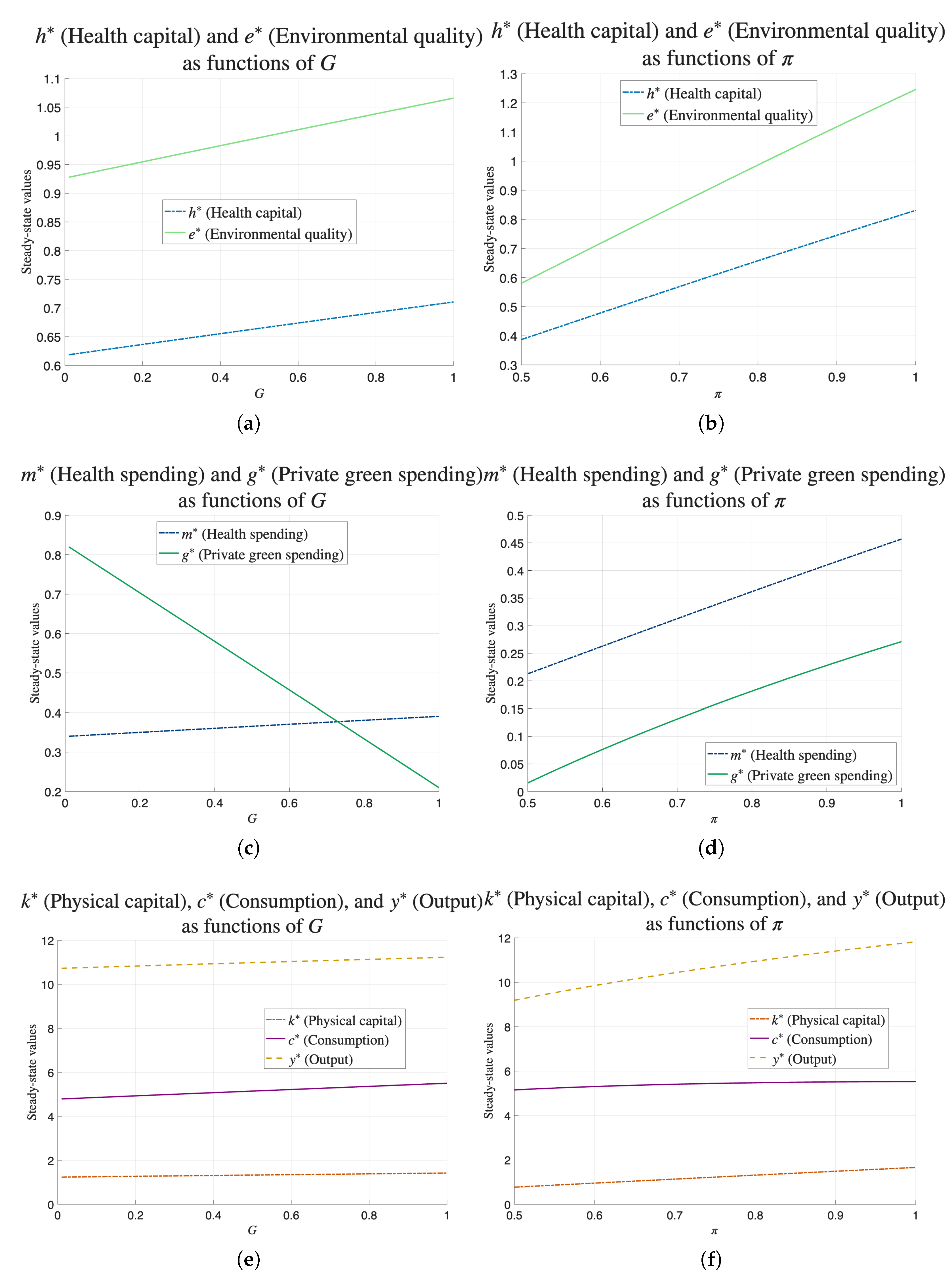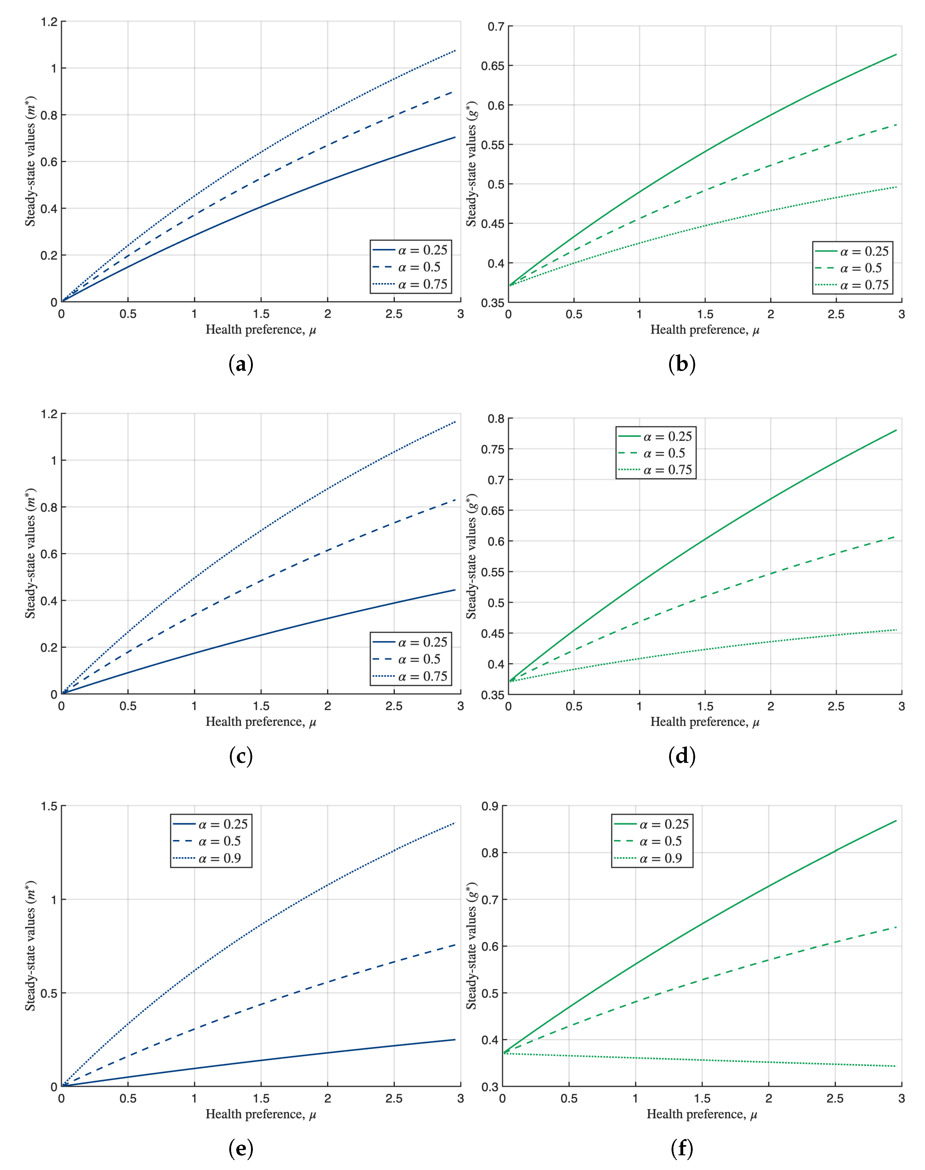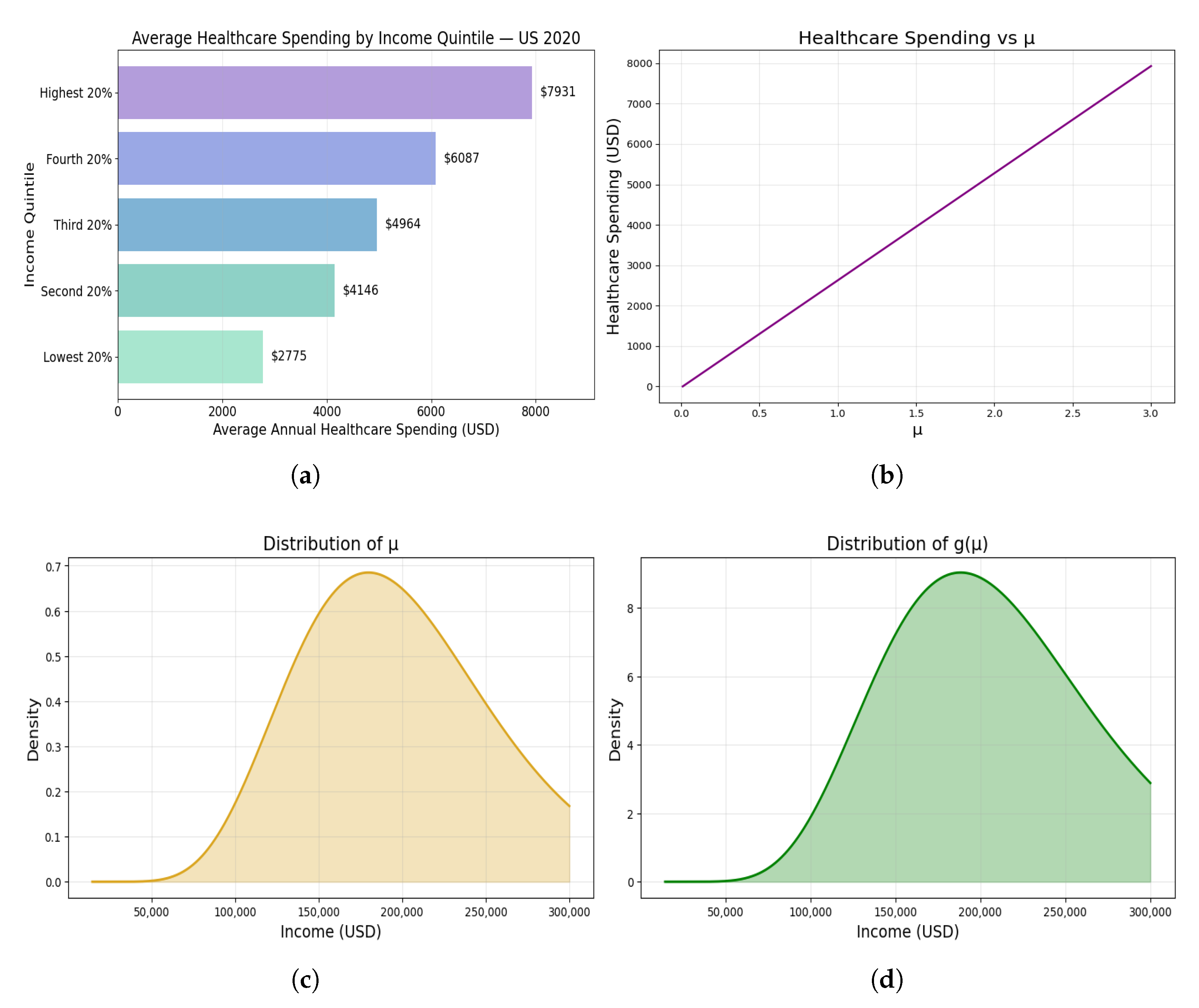The effects of other parameters and all formal derivations are relegated to Appendix B. 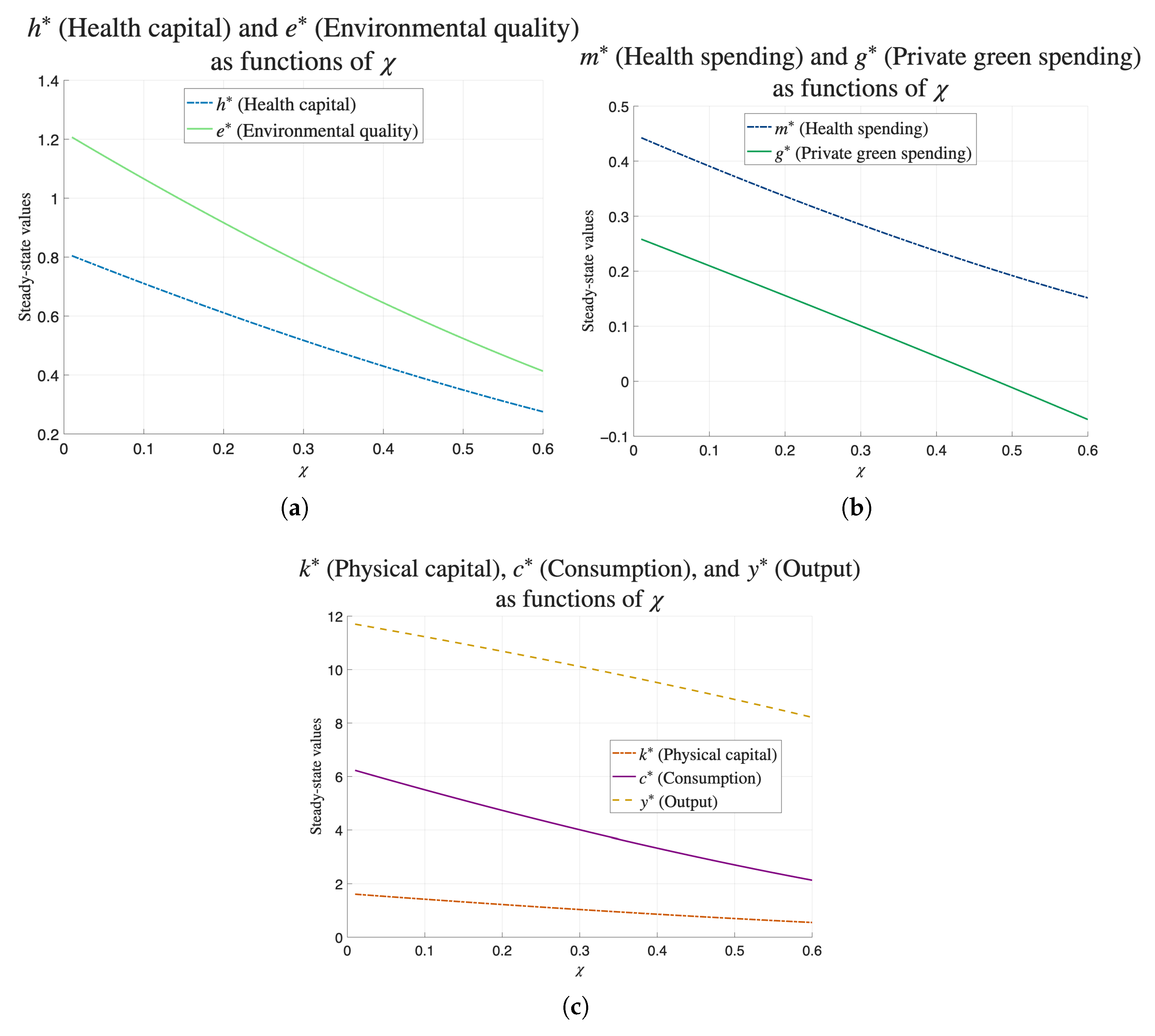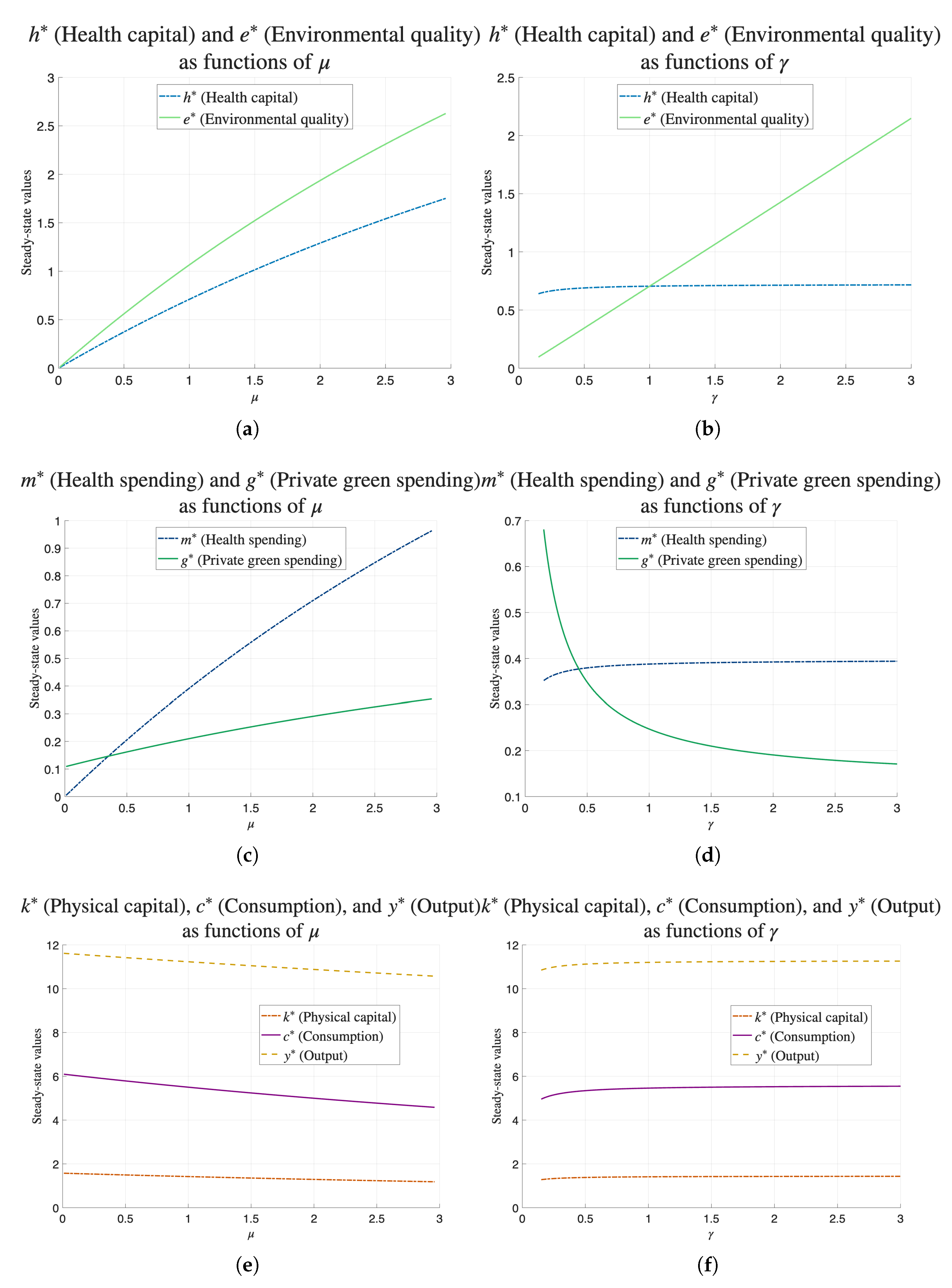We complement analytical results with a set of numerical simulations shown in Figure 1 and Figure 2 as well as in Figure A1 in Appendix C. These numerical exercises are meant to visualize key qualitative relationships rather than provide quantitative predictions. The parameter values underlying the simulations are provided in

Table A1. Choice of parameter values for model simulations (full period length = 40 years).

Parameter	Value	Description	Source
A	10.0	Total factor productivity	[34]
$\alpha$	0.5	Cobb–Douglas health elasticity parameter	Assumption, relaxed in CES extension
$\gamma$	1.5	Effectiveness of private green investment	Assumption, relaxed in comparative statics
$\Gamma$	1.0	Effectiveness of public green investment	Normalization
$\delta$	0.55	Rate of health decay	Aging of 2% per year, average of estimates in the literature [55,56,57,58,59]
$\eta$	0.18	Rate of environmental destruction	Following the methodology in [37] for a yearly rate of 0.005
$\theta$	0.33	Cobb–Douglas capital elasticity parameter	Standard economic assumption
$\mu$	1.0	Concern for own health	Assumption, relaxed in comparative statics
$\nu$	1.0	Rate of physical capital destruction	Full depreciation assumption, see [34,60]
$\pi$	0.86	Survival probability	Following the average probability of a 30-year-old individual surviving until 70 years old in Austria (life expectancy calculator at [61])
$\rho$	2.33	Time discount rate	Following [34,60]
$\chi$	0.1	Polluting intensity of production	Following [34]
G	1	Public green spending	Normalization

Following the structure of the model (e.g., non-negativity of capital in the steady state) and assumptions common in economic theory, we set these parameter values for illustrative purposes.

.

4.1. Physical Capital ($k^{*}$)

By totally differentiating Equation (16), we obtain

$$\begin{array}{c}\hfill {\Delta }_{k}d{k}^{*}={\Delta }_{\pi }d\pi +{\Delta }_{\mu }d\mu +{\Delta }_{\gamma }d\gamma +{\Delta }_{G}dG+{\Delta }_{\chi }d\chi ,\end{array}$$

(23)

where

$$\begin{array}{ccc}& & {\Delta }_k=1-D\Omega -D(1-\theta -\chi /\gamma )y^{{*}^{\prime }}>0,\hfill \end{array}$$

(24)

$$\begin{array}{ccc}& & {\Delta }_{\pi }={\displaystyle \frac{\mathsf{\partial }D}{\mathsf{\partial }B}}{\displaystyle \frac{\mathsf{\partial }B}{\mathsf{\partial }\pi }}\left((1-\theta -\chi /\gamma )y^{*}+k^{*}\Omega +{\displaystyle \frac{\Gamma }{\gamma }}G\right)>0,\hfill \end{array}$$

(25)

$$\begin{array}{ccc}& & {\Delta }_{\mu }={\displaystyle \frac{\mathsf{\partial }D}{\mathsf{\partial }\mu }}\left((1-\theta -\chi /\gamma )y^{*}+k^{*}\Omega +{\displaystyle \frac{\Gamma }{\gamma }}G\right)+k^{*}D{\displaystyle \frac{\mathsf{\partial }\Omega }{\mathsf{\partial }\mu }}<0,\hfill \end{array}$$

(26)

$$\begin{array}{ccc}& & {\Delta }_{\gamma }={\displaystyle \frac{D}{{\gamma }^2}}(\chi y^{*}-\Gamma G)>0,\hfill \end{array}$$

(27)

$$\begin{array}{ccc}& & {\Delta }_G={\displaystyle \frac{D\Gamma }{\gamma }}>0,\hfill \end{array}$$

(28)

$$\begin{array}{ccc}& & {\Delta }_{\chi }=-{\displaystyle \frac{D{y}^{*}}{\gamma }}<0,\hfill \end{array}$$

(29)

and $B={\displaystyle \frac{\pi }{1+\rho }}$, $D={\displaystyle \frac{B}{\nu [1+(1+\mu \left)B\right]}}$, $\Omega =\mu \nu \left[\right(1-\delta )\alpha +(1-\eta \left)\right(1-\alpha \left)\right]$. We can therefore derive the following comparative statistical results with respect to our main parameters of interest: A higher survival probability has a positive effect on the steady-state capital stock, as illustrated in Figure 2f. This is because a larger $\pi$ increases the saving rate by Equation (11), which then directly feeds into the capital stock by Equation (14). Conversely, a stronger health preference reduces the steady-state capital stock, as shown in Figure 1e, because it diverts resources from capital accumulation towards investment in health by Equation (9) but also towards green investment by Equation (10). Overall, the share $\mu$ of total savings is split between health and green investments in the proportion $\alpha$ and $1-\alpha$, respectively, which are exactly the respective shares of health stock and environmental quality entering the health status composite in Equation (3). The effect of individual green investment productivity, $\gamma$, on the steady-state capital stock is positive, as can be seen in Figure 1f. This is because a higher $\gamma$ reduces the need for green investments, all else equal, and thus frees up resources for capital build-up. Finally, the government contribution to a better environmental quality, G, also has a positive effect on $k^{*}$ (Figure 2e) and follows a similar intuition as the effect of $\gamma$, since both enter the law of motion for e, Equation (1), in a similar way.

The effects on the remaining endogenous variables will be analyzed using the established comparative statistical results for $k^{*}$.

4.2. Young-Age Consumption ($c^{*})$

From Equation (19) (see also Appendix A), we know that steady-state consumption is proportional to the capital stock: $c^{*}={\displaystyle \frac{\nu k^{*}}{B}}={\displaystyle \frac{\nu k^{*}(1+\rho )}{\pi }}$. Hence, the directions of the effects of our parameters of interest remain unaltered as compared with those for $k^{*}$, except for the survival probability $\pi$, as follows:

$$\begin{array}{ccc}& & {\displaystyle \frac{d{c}^{*}}{d\pi }}={\displaystyle \frac{\nu (1+\rho )}{{\pi }^2}}\left[\pi {\displaystyle \frac{{\Delta }_{\pi }}{{\Delta }_k}}-k^{*}\right]\gtrless 0.\hfill \end{array}$$

(30)

The economic interpretation of these results follows the same intuition as already discussed for $k^{*}$, except again for the survival probability, which exerts both a direct and an indirect effect on $c^{*}$. The indirect effect works through the capital stock and is positive. The direct effect is negative because a higher probability of surviving to old age increases the need to save and therefore reduces the current consumption. The total effect on $c^{*}$ depends on the magnitude of the elasticity of $k^{*}$ with respect to $\pi$. To see this, rewrite the term in the square brackets in (30) as $k^{*}\left[{\displaystyle \frac{\pi }{k^{*}}}{\displaystyle \frac{d{k}^{*}}{d\pi }}-1\right]=k^{*}\left[{\epsilon }_{k\pi }-1\right]$, where ${\epsilon }_{k\pi }$ is the elasticity of $k^{*}$ with respect to $\pi$. If the value of this elasticity exceeds unity, ${\displaystyle \frac{d{c}^{*}}{d\pi }}>0$, and vice versa. Our simulations reveal that the value of ${\epsilon }_{k\pi }$ is above unity for the empirically relevant range of model parameters, and therefore, ${\displaystyle \frac{d{c}^{*}}{d\pi }}>0$; i.e., the indirect positive effect dominates (see Figure 2f).

4.3. Old-Age Consumption ($d^{*})$

The old-age consumption is simply equal to the savings plus the accumulated interest. It follows from Equation (20) that $d^{*}$ is an increasing function of $k^{*}$; the comparative statics of the old-age consumption and physical capital with respect to our parameters of interest have therefore identical signs.

4.4. Environmental Quality ($e^{*}$)

By differentiating Equation (17), we obtain that because the steady-state level of environmental quality increases in $k^{*}$ (and in $\gamma$), the comparative statistical results with respect to $\pi$, $\gamma$, and G have identical signs to the comparative statistical results for physical capital $k^{*}$, with the same underlying intuition. Figure 1b and Figure 2a,b illustrate these effects. Only the effect of the health preference, $\mu$, is ambiguous. This ambiguity stems from the counteracting forces of the direct positive effect and the indirect negative effect working through $k^{*}$. It can be shown, however (see Appendix B), that the direct effect dominates and environmental quality increases in health preference (see Figure 1a). Recall that a fraction $\mu$ of total savings is devoted to investments in own health stock and into individual environmental improvements (with a fraction $\alpha$ going to the former and $1-\alpha$ to the latter). Hence, a marginally higher $\mu$ increases $e^{*}$ by $(1-\alpha )\gamma \nu k^{*}$ directly. At the same time, a higher $\mu$ diverts resources from capital accumulation, $d{k}^{*}/d\mu <0$, and thus reduces the overall savings. However, it can be shown that the elasticity of $k^{*}$ with respect to $\mu$ is smaller than unity, and thus, the diversion effect is smaller in absolute value than the direct effect. Therefore, the positive effect outweighs the negative one.

4.5. Health Capital ($h^{*}$)

By totally differentiating Equation (18), we obtain the comparative statistical results for intrinsic health stock $h^{*}$ in steady state. The directions of the effects on the health stock are identical to those for environmental quality and follow the same intuitive explanations. Figure 1a,b and Figure 2a,b provide illustrations. These results highlight the similarity of the effects of own intrinsic health and the environment in determining individual behavior and optimal responses. Quantitatively, the results differ because $e^{*}$ depends directly on the private abatement efficiency $\gamma$, while $h^{*}$ does not, and because of the difference in the share of the total savings devoted to the respective private investments (g and m), determined by the fractions $1-\alpha$ and $\alpha$, respectively.

4.6. Health Spending ($m^{*}$)

It follows from Equation (21) that the steady-state level of private investment in health is a constant fraction $\delta$ of the health stock: $m^{*}=\delta h^{*}$. Since $\delta >0$, the signs of the comparative statistical results for $m^{*}$ with respect to all the parameters of interest coincide with those for the health capital $h^{*}$. The fact that an individual investment in own health capital increases with the health preference $\mu$ and with the survival probability $\pi$ is rather intuitive (Figure 1c and Figure 2d). What is less obvious is that a higher individual productivity of environmental investment, $\gamma$, and a higher government support for the environment, G, also lead to a higher investment in own health. Both $\gamma$ and G contribute to a better environmental quality (Equation (1)), all else equal (see Figure 1b and Figure 2d), and therefore reduce the need for an individual green investment, akin to a crowding-out effect. However, that increases the resources available for capital accumulation, which leads to higher overall steady-state savings and capital stock and thus higher overall resources available for health investment. These results highlight the important interactions between investments in environmental protection, both private and public, and individuals’ decisions to invest in their own health. By supporting environmental action, public policy can indirectly positively influence individuals’ pro-health-oriented choices and thereby improve the overall health status on both margins, i.e., by boosting e and h. Moreover, by facilitating and improving the effectiveness of individual green action, the government can additionally boost m, h, and by extension, H. Although we do not model explicitly any public health policies, our results suggest that there are potentially important and sizable synergy effects between public health and environmental policies (relevant policies at the intersection of environmental and health concerns are analyzed in applied economic literature, for example [50,51,52]).

4.7. Private Green Investment ($g^{*}$)

From Equation (22), we know that the survival probability affects the steady-state individual green investment only indirectly, through the capital stock, while the health preference parameter, the private green efficiency, and government policy have direct and indirect effects.

The only unambiguous effect concerns the survival probability. A higher $\pi$ works to raise the steady-state capital and therefore indirectly increases the green investment as well, as illustrated in Figure 2d. The effect of the private green investment efficiency is ambiguous and has to do with the interplay between a positive effect on the steady-state capital and a negative “rebound effect”, by which we mean a reduction in the absolute level of investment when the effectiveness of this investment in improving environmental quality rises (the rebound effect was initially documented in the energy economics literature and refers to the phenomenon where improvements in energy efficiency lead to less reduction in energy consumption than expected because agents change their behavior in response to the efficiency gain; see, e.g., [53,54]). Our simulations show that, for an empirically relevant range of model parameters, the rebound effect dominates, and therefore, the private green investment decreases in $\gamma$ (Figure 1d).

Government-financed climate policy also has an ambiguous effect on $g^{*}$, reflecting the counteracting forces of the positive effect on the steady-state capital and a direct negative crowding-out effect. Our simulations in Figure 2c show that the crowding-out effect dominates; i.e., the private green investment falls as G increases. However, the overall environmental quality increases in G, as can be seen in Figure 2a, implying that the government green spending more than compensates for a decline in private green contributions.

Finally, when it comes to the health preference, we see in Figure 1c that $g^{*}$ increases in $\mu$. Therefore, a stronger concern for own health incentivizes individuals to do more private green investments (along with more investment in own health). This suggests that a public policy promoting health consciousness of individuals has a potential to enhance private green contributions and ultimately the overall environmental quality. A clear advantage of such a policy, e.g., public educational campaigns raising population awareness about exposure to pollution and harmful substances, can be much more readily internalized by individuals, as compared with pollution taxes or even mere environmental nudging.

5. Environmental Policy

In this section, we describe how the government determines its policy G. Suppose that the government sets a tax $\tau \in [0,1)$ on output and uses the proceeds from taxation to finance the environmental policy, as follows:

$$G_t=\tau y_t=\tau A{k}_t^{\theta }.$$

(31)

The factor returns will therefore be adjusted by the factor $1-\tau$; i.e., they will be after-tax returns. This modification of the model introduces changes to only two steady-state equations: the household’s budget constraint and environmental quality (see Appendix D). Taking these modifications into account, we obtain the steady-state level of the capital stock as

$$k^{*EP}={\left\{{\displaystyle \frac{A\left[(1-\tau )(1-\theta )+\frac{\Gamma \tau -\chi }{\gamma }\right]}{\nu \left[1+\frac{1}{B}+\eta (1-\alpha )\mu +\delta \alpha \mu \right]}}\right\}}^{{\displaystyle \frac{1}{1-\theta }}}.$$

(32)

The environmental tax exerts two opposing forces on the level of $k^{*EP}$. On the one hand, it works to reduce $k^{*EP}$ by having a negative effect on the wage rate—recall that both factor returns are reduced by a factor $1-\tau$. This effect is given by the first term in the square brackets in the numerator of (32). On the other hand, the environmental policy improves the state of the environment and thus reduces the need for private green investment, liberating savings for capital accumulation (the crowding-out)—the positive effect given by the $\Gamma \tau /\gamma$ term in the numerator. The extent to which the tax works to increase $k^{*EP}$ depends on the relative effectiveness of the government vs private intervention ($\Gamma /\gamma$). One can verify that, by setting $\tau =0$, we recover the solution for our steady-state capital of the benchmark model without the government ($G=0$), given in Equation (A20) in the appendix.

The steady-state values of the remaining endogenous variables can be computed using (32)

$$\begin{array}{cc}\hfill & c^{*}={\displaystyle \frac{\nu }{B}}{k}^{*EP},\hfill \end{array}$$

(33)

$$\begin{array}{cc}\hfill & h^{*}=\alpha \mu s^{*}=\alpha \mu B{c}^{*},\hfill \end{array}$$

(34)

$$\begin{array}{cc}\hfill & e^{*}=\gamma (1-\alpha )\mu B{c}^{*},\hfill \end{array}$$

(35)

$$\begin{array}{cc}\hfill & m^{*}=\delta h^{*},\hfill \end{array}$$

(36)

$$\begin{array}{cc}\hfill & g^{*}={\displaystyle \frac{\eta (1-\alpha )}{\alpha }}{h}^{*}-{\displaystyle \frac{\Gamma \tau -\chi }{\gamma }}A{\left(k^{*EP}\right)}^{\theta }.\hfill \end{array}$$

(37)

6. Policy Implications: Activating Private Green Investment Through Health Channels

The results of the model suggest that environmental policy can be substantially reinforced by instruments that operate through individuals’ concern for their own health. In contrast with conventional approaches that rely primarily on taxation or regulation, health-oriented policies influence behavior by increasing the perceived private returns to environmental quality. This section outlines a set of policy-relevant implications and discusses the associated trade-offs.

First, the model highlights the potential effectiveness of health-centered environmental information policies. Public information campaigns that clearly communicate the long-term health consequences of environmental degradation—such as air pollution, chemical exposure, or microplastic contamination—can raise individuals’ concern for future health. Importantly, this mechanism relies on voluntary behavioral responses rather than coercive measures. To maximize effectiveness, information should emphasize concrete exposure-health pathways (e.g., air pollution is associated with cardiovascular risks; microplastics exposure has implications for fertility and inflammation), life-cycle health impacts, and the limited substitutability between intrinsic health investments and environmental quality. A key trade-off is that such campaigns may be more readily internalized by highly educated or health-literate individuals, potentially widening behavioral and health disparities unless complemented by targeted outreach to vulnerable groups.

Second, mandatory disclosure of environmental health impacts emerges as a powerful complement to general information campaigns. Standardized disclosure requirements—such as pollution intensity labels, toxicity scores, or environmental health footprints of consumer goods and buildings—can increase the salience of environmental quality in individual decision making. By lowering information costs and improving risk perception, disclosure policies strengthen incentives for private green investment without directly restricting individuals’ choice. However, disclosure regimes entail compliance costs for firms and may generate information overload if poorly designed. Moreover, low-income households may face constrained choices even when information is improved, implying that disclosure alone is unlikely to be distribution-neutral.

Third, the analysis supports targeted subsidies for household-level green technologies with health co-benefits, including indoor air filtration, low-toxicity materials, and water purification systems. In the model, policies that raise the effectiveness of private environmental investment ($\gamma$) increase environmental quality and health capital, even when they reduce the absolute level of private green spending due to rebound effects. From a welfare perspective, the net environmental and health gains dominate. Targeting such subsidies towards high-exposure or low-income households can mitigate environmental health inequalities. The main trade-offs concern fiscal cost, administrative complexity, and the risk that efficiency gains reduce incentives for continued private effort.

Fourth, localized environmental health reporting can strengthen individual incentives by linking pollution exposure to place-based health risks. High-resolution pollution–health dashboards or neighborhood-level exposure indicators increase the perceived relevance of environmental quality for those most affected. In a framework where environmental quality enters health status directly, such localization enhances the behavioral response of exposed individuals and can stimulate both private action and political support for public abatement. At the same time, localized disclosure may induce unintended effects, such as residential sorting, stigmatization of polluted areas, or political resistance from affected industries.

Finally, the results point to important synergies between preventive healthcare policy and environmental policy. When evaluating impacts of environmental policies, e.g., carbon pricing, health co-benefits should be factored in. Likewise, integrating environmental risk reduction into healthcare systems—for example, through exposure screening, physician counseling, or insurance incentives—reinforces the complementarity between health investment and environmental quality. Although the model abstracts from explicit healthcare provision, the comparative statics show that improvements in environmental quality and survival probability jointly raise health investment and long-run welfare. A potential concern is that such integration may overburden healthcare systems or benefit primarily higher-income individuals unless access is universal.

Taken together, these implications suggest that an effective sustainability-oriented policy mix should combine (i) instruments that raise health awareness and concern, (ii) measures that enhance the effectiveness of private green action, and (iii) public environmental investment that compensates for distributional asymmetries in exposure and income. While health-based information and disclosure policies can mobilize private environmental effort at relatively low fiscal cost, they are not distribution-neutral. Without complementary public abatement and targeted support, they risk amplifying existing inequalities in health and environmental exposure. The model thus underscores the importance of designing environmental policies that leverage individual self-interest while maintaining equity and intergenerational sustainability.

7. Discussion and Outlook

This paper develops a unified overlapping generations framework that links individual health attitudes, health capital formation, and environmental quality. We offer a novel integration of health stock and environmental quality into a composite health status. The distinction between intrinsic health and the environmentally augmented health status is particularly important. It reflects the current scientific understanding that environmental exposures can undermine even substantial individual investment in lifestyle and health behaviors. This modeling innovation enhances ecological realism in growth theory. The results provide several insights of direct relevance for public policy and sustainability. Above all, the model demonstrates that individuals who attach greater importance to their own long-term health engage in higher private environmental investment, which in turn improves both environmental quality and their eventual health status. This mechanism highlights an important but underexplored channel through which population health preferences can influence environmental outcomes: the internalization of environmental risks through personal health motives. In contrast with policy instruments that rely on external enforcement or financial incentives, health-driven behavioral responses emerge voluntarily. This suggests a considerable untapped mitigation potential originating from health awareness and risk perception.

First, the model implies that policies that elevate awareness of environmental health risks—for example, through science-based public information campaigns, disclosure requirements, chemical risk labeling, or environmental health education—may have substantial positive effects on environmental quality. By increasing individuals’ health concern, such interventions encourage both higher private spending on environmental protection and greater investment in intrinsic health capital. These channels work jointly to strengthen human and environmental resilience.

Second, the results reveal important complementarities between public and private environmental action. Government abatement spending improves steady-state environmental quality and increases individuals’ capacity to invest in their own health by easing the need for private green spending. This interaction reduces total environmental degradation while simultaneously raising health stocks. Importantly, although government intervention may crowd out private green investment in absolute terms, the net environmental effect remains strictly positive. This suggests that public environmental policy and individual behavioral responses need not be considered substitutes; rather, they form a mutually reinforcing policy mix.

Third, the model highlights that improvements in the efficiency of green technologies (e.g., more effective household-level air filtration, cleaner consumer products, low-toxicity materials, or affordable pollution-abatement devices) raise environmental quality not only directly but also indirectly through their impact on savings and health investment. These findings argue in favor of policies supporting innovation in environmental technologies, regulatory standards for product safety, and accelerated diffusion of low-emission technologies at the household level.

Fourth, because survival probability enhances savings and indirectly raises both private environmental and health investment, our results suggest that public health interventions that raise life expectancy—including healthcare access, preventive medicine, and pollution-reduction measures—have long-run macroeconomic benefits. They stimulate capital accumulation and increase resources available for sustainable behavior. This reaffirms the importance of viewing public health policy and environmental policy as interdependent rather than separate domains.

Our findings underscore the bidirectional link between environmental sustainability and human health sustainability. The model shows that the sustainability of human health cannot be ensured if environmental degradation persists, because health status depends simultaneously on intrinsic health capital and environmental quality, both of them being essential. This complements the empirical evidence presented in the Introduction and confirms analytically that health-oriented sustainability strategies must account for environmental exposures, pollution stocks, and long-term deterioration dynamics.

In the broader context of sustainable development, our results showcase several layers of relevance. First, the intergenerational sustainability: Environmental quality and health capital are transmitted intertemporally in the model, meaning that the welfare of future generations depends critically on today’s environmental policies and health behaviors. This aligns directly with the logic of the Sustainable Development Goals, especially SDGs 3 (health), 6 (water), 11 (cities), and 13 (climate). Second, behavioral sustainability: As individuals with stronger health motivations invest more in environmental protection, population-level sustainability outcomes may depend on societal trends in health awareness, education, and risk perception. These behavioral factors represent an endogenous driver of environmental sustainability that is often absent from macroeconomic models.

Our model also contributes to the understanding of the synergies and trade-offs between SDG3 (Good Health and Well-being) and SDG13 (Climate Action). By modeling health status as jointly determined by intrinsic health stock and environmental quality, the analysis formally demonstrates that sustained improvements in population health are not feasible under persistent environmental degradation. Climate and pollution mitigation therefore not only represent environmental objectives but are also structural determinants of long-run health outcomes. At the same time, the model highlights that the capacity to translate health concerns into private environmental investment depends on economic resources and institutional context. In lower-income countries, where disposable income and access to green technologies are limited and pollution intensity may be high, private environmental investment is likely to be constrained despite potentially large health gains from environmental improvement. In contrast, higher-income economies may exhibit stronger voluntary environmental responses but face diminishing marginal health returns. These asymmetries imply that achieving SDG3 and SDG13 jointly requires differentiated policy mixes: public abatement and international financial support are particularly critical in early stages of development, whereas information-based instruments and efficiency-enhancing policies may play a larger role in advanced economies. The model thus highlights that health and climate objectives are structurally complementary, but their effective integration depends on development-specific constraints and capacities.

Future work could adopt several extensions. Endogenizing survival probability would allow analysis of how environmental improvements feed back into longevity and savings decisions. Incorporating heterogeneity in education or income would permit the evaluation of distributional consequences and environmental justice aspects. While the analysis focuses on long-run steady states and comparative statics, the framework can naturally be extended to study transitional dynamics and shocks. Sudden environmental events (e.g., pollution spikes, climate-related disasters), health shocks (e.g., pandemics), or abrupt policy changes (e.g., regulatory tightening) can be modeled as unanticipated shifts in key parameters such as pollution intensity, environmental efficiency, survival probability, or health preferences. These shocks would generate transitional paths in health investment, private green effort, and capital accumulation before the economy converges to a new steady state. Importantly, the model’s structure implies that shocks affecting environmental quality may have persistent effects through their impact on health status and future behavior, potentially amplifying short-run disturbances into long-run health and environmental disparities. Conversely, health-related shocks that increase risk awareness may permanently raise private environmental investment by shifting health preferences. Analyzing such dynamics would require introducing expectations and adjustment frictions, which is beyond the scope of the present paper but represents a promising direction for future research. The steady-state results presented here provide a benchmark against which the long-run consequences of repeated or persistent shocks can be evaluated. Finally, coupling the model with empirical calibration or structural estimation would enable quantitative assessment of environmental health policy scenarios.