A Comprehensive Approach to Defining the Cost of Inventory Management: A Case Study on Small Batch Cargo Delivery

Abstract

In recent years, there has been a significant negative impact on the sustainability of supply chains for the delivery of small batch cargo, caused by crisis situations. Therefore, it is important to develop a modern methodology to reduce uncertainty in the delivery of small batch cargo, especially when considering a flexible inventory management system. This study proposes an integrated approach to inventory management, consisting of three elements: an updated ABC-XYZ structure of inventory formation analysis with criteria that determine stability; an additive mathematical model for calculating inventory management costs; and the development of a regression model for operational forecasting of inventory management costs, based on the number of end customers, unit cost and batch size. A comparison of regressions showed the advantage of the power model over the linear one. The main advantage of the study is the proposed mathematical and regression models for the operational calculation of inventory management costs, considering the uncertainty factors that determine the sustainability of the supply chain. This approach will be of interest to trading enterprises, allowing them to make flexible decisions in inventory management in the event of various disruptions in small batch cargo supply chains.

1. Introduction

Inventory management remains one of the key challenges of supply chains, directly affecting their sustainability and efficiency [1,2]. In recent years, global crises, including the COVID-19 pandemic, economic turmoil, and geopolitical conflicts, have significantly complicated small batch cargo delivery processes [3,4]. Unstable demand for the delivery of small shipments and rising unexpected costs associated with logistics disruptions have increased uncertainty and revealed the limitations of traditional approaches [5,6,7,8].

Modern research in the field of inventory management is developing in several directions. One of them is related to the improvement of classification methods, i.e., selecting the best product groups according to certain criteria [9]. Classic ABC-XYZ analysis is still used in practice, but its application is limited because it primarily considers cost and demand variability, ignoring the strategic importance of products and their role in maintaining supply chain sustainability [10,11]. Attempts to extend ABC-XYZ through multi-criteria models have been made, but they are rarely integrated with costing and therefore have limited applicability in the sector [12].

Another area of research is related to cost modeling and demand forecasting. However, machine learning methods and hybrid statistical approaches are commonly used to improve the accuracy of forecasts of intermittent and unstable demand [13,14,15]. In addition, economic and mathematical models of cost management, including deterministic and stochastic ones, have been proposed [16,17]. However, their main limitation is that they focus either on the forecasting or optimization of individual costs, without combining classification and cost analysis into a single methodology.

A key area is related to the resilience of supply chains in times of crisis. Thus, digital twins and simulation models make it possible to predict failures at the macro level [1,18]. However, the operational level—the inventory management in small batch cargo deliveries—remains underdeveloped [19,20,21]. At the same time, micro-level processes have a decisive influence on the flexibility and adaptability of logistics and warehouse systems in the face of disruptions [22,23].

Thus, a situation arises in which inventory classification methods have limited relevance to costs, cost models do not consider the multidimensionality of inventory characteristics, and sustainability studies bypass the issue at the operational level. This creates a knowledge gap: there is no comprehensive methodology that can combine modified ABC-XYZ analysis and economic and mathematical modeling of costs in conditions of unstable demand and logistics failures.

Unlike existing studies that consider segmentation, cost accounting, and forecasting separately, this paper proposes an integrated, reproducible workflow that links strategic inventory segmentation to operational cost estimation. Importantly, the contribution is not a new use of ABC-XYZ, costing, or regression in isolation, but a parameterized decision-rule extension of ABC-XYZ (inventory turnover–goods significance–demand sustainability (IT-GS-DS) with explicit percentile, share, coefficient of variation (CV) cutoffs) and its direct coupling to a transparent cost response function and elasticity-based forecasting for operational what-if analysis. The workflow combines modified ABC-XYZ segmentation enriched with sustainability criteria, an interpretable additive cost decomposition, and a power-law regression model that provides elasticities and enables quick what-if forecasting. Supporting steps include Likert-based expert screening for selecting controllable inputs and a full-factorial 2 × 2 × 2 design that generates reproducible calibration points for regression estimation. This addresses a key gap in the current literature between building a warehouse inventory segment and controlling inventory holding costs. Therefore, the methodology allows us to quantitatively determine the optimal batch size g and form a priority set of customers n based on fluctuations in demand and external compensation, ensuring the sustainability of supply logistics and prompt decision-making.

To address the above knowledge gap, the following research question (RQ1) is intended to be addressed: how can the integration of modified ABC-XYZ analysis and economic–mathematical cost models improve the sustainability of small batch cargo supply chains?

To answer this question, the study proposes a unique additive model for calculating inventory holding costs, including warehouse maintenance costs, storage costs, warehouse operations, and capital freezing costs. This multifactorial approach takes into account the key cost elements that form the total costs. Additionally, regression analysis was carried out to predict costs, depending on the number of end customers, the average cost of a unit of production and the size of the delivery batch. The approach is unique in that it combines strategic inventory segmentation and cost quantification with high forecasting accuracy supported by appropriate relative error validation.

The practical significance of the study lies in the fact that the proposed methodology can be directly used by retail chains and distribution centers working with small batch cargo deliveries. This approach enables enterprises to reduce costs while strengthening the resilience and stability of the inventory management system.

The paper is organized as follows. Section 2 reviews approaches to inventory segmentation and inventory cost estimation. Section 3 presents the proposed methodology, including the modified ABC-XYZ criteria, deterministic cost model, expert-based factor screening, and regression specification and validation. Section 4 reports the case study results and sensitivity analysis. Section 5 discusses the implications and limitations, and outlines future research.

2. Literature Review

This section provides an overview of the existing approaches to the need to create inventories of goods based on ABC-XYZ analysis and other common approaches (Section 2.1). A review of methods and models for calculating inventory holding costs was also carried out, identifying their main advantages and disadvantages (Section 2.2).

2.1. Existing Approaches to Defining Inventory Rate

Traditional inventory management approaches, based on Wilson’s classic EOQ (economic order quantity) formula, minimize the total annual costs [24,25]. This approach provides quick and informative solutions for items with stable demand and enables the interpretation of parameters’ influence (order cost, unit storage costs, etc.). Models with a fixed order size and time interval between orders are often not efficient enough for specific logistics operations [26,27,28]. This is because they do not always adequately account for the high variability of demand, short order cycles and significant operating costs associated with delivering small batches of cargo.

The continuous inventory control method is considered one of the basic inventory management strategies [29]. This method quickly responds to changes in demand while maintaining the minimum required inventory level, which is particularly crucial for high-value products or when demand is highly variable. The authors note that the implementation of a continuous monitoring system requires significant investment in modern software (for example, warehouse management systems) and equipment for automatic data collection [30]. This can be overwhelming for small and medium-sized businesses. Constant monitoring results in frequent but small orders, which can significantly increase logistics and transportation costs, especially if suppliers charge high processing fees for each individual order [31]. This may offset savings from reduced storage costs.

The opposite of the continuous control method is the periodic review method, also known as policy (R, T) or “order-up-to/periodic review.” It is easier to administer, because it does not require constant monitoring. It is typically used for low-value products, stable demand, or situations where logistics operations (such as shipping) can be combined across multiple items [32,33]. Since inventory levels are not continuously monitored using this method, there is a risk of stockouts. To avoid this, it is necessary to maintain a higher level of safety stock, which increases storage costs. There is also the possibility of an inaccurate EOQ calculation. The order size depends on the current inventory levels, which prevents firms from consistently using the economic order quantity (EOQ). This may result in suboptimal costs [34,35].

One of the most common methods in logistics is the method of calculating safety stock based on service level. Its essence is to determine the amount of additional inventory needed to satisfy customer demand for a certain percentage of the time [36]. The method is based on statistical laws, which makes it more objective and accurate compared to empirical or expert approaches. This allows companies to consciously manage inventory by choosing a service level that meets its strategic goals and financial capabilities [37]. The method is effective only if reliable and historical data on demand and order lead time are available. Inaccurate or incomplete data can lead to significant calculation errors [38,39]. For beginners or businesses without specialized software, the calculations may seem complicated, as they require knowledge of statistical tools.

The differentiated inventory management policy method (ABC-XYZ classification) enables focusing efforts on the most important positions (group A), which generate the main income, without spending extra time and resources on less important goods (group C). A differentiated approach helps to reduce inventory holding costs through more accurate forecasting for X groups and simplified management for Z groups, and the application of individual strategies for each group makes it possible to increase the availability of critical goods (AX, AY) for customers [40,41]. Implementation of the method requires the collection of substantial amounts of data and the calculation of the coefficients of variation and analysis, and the dynamic nature of the classification requires regular review and updating of the classification, which requires additional resources [42,43]. The method may be less effective for companies where all products have approximately the same value or have very unstable demand [44]. The main difference from deterministic models (like EOQ) of the stochastic/optimization approach as an inventory management method is that stochastic models treat demand or delivery time as random variables (stochastic), rather than as constants [45]. These models focus on cost optimization (minimizing the total costs of storage, ordering, and stockouts) while considering probabilistic features [46]. Accurate modeling requires enormous amounts of reliable historical data on demand and delivery times, which is not always available. Poor-quality data can lead to suboptimal decisions [47,48].

Forecasting and machine learning models are a promising approach to inventory management that differ from traditional statistical methods in that they use sophisticated algorithms to analyze large volumes of data [49]. These models go beyond simply calculating averages to discover hidden patterns in consumer demand and behavior. With this, they can make more accurate predictions [50,51]. To train and effectively operate this type of model, large volumes of high-quality structured data are required. Insufficient quantity or poor quality of data can lead to inaccurate forecasts. Some complex models (especially deep neural networks) can be uninterpretable, meaning it is difficult to understand what factors the model used to make a particular decision. This makes it difficult to trust the system and analyze errors.

The Just-in-Time (JIT) and Lean approach to inventory management is a philosophy aimed at minimizing all types of waste, including excess inventory. According to the JIT approach, inventories are treated as waste and should be minimized [52]. In practice, lean routines (e.g., 5S standardization) are often disseminated through staff workshops; virtual reality training has been reported to increase workshop effectiveness and support more consistent adoption of lean practices [53]. The “zero inventory” policy is the idealized end result of JIT and Lean implementation. It assumes minimal or, ideally, complete absence of inventories both in the finished goods warehouse and at all stages of production [54,55]. Any delay in supply, unpredictable disruption in production or fluctuations in demand can bring the entire production process to a standstill [56]. Lack of safety stock is the biggest risk. The success of JIT implementation depends on the reliability and punctuality of suppliers, as well as their willingness to deliver frequently and in small quantities [56]. This requires close integration and collaboration.

The simulation approach to inventory management is a method that uses computer models to simulate actual logistics processes over a specified period. It enables analyzing the behavior of a system under different conditions that are difficult or impossible to reproduce in reality. This approach is particularly useful when the system is extremely complex and demand and supply timing are highly uncertain [57,58]. “What-if” analysis is a key part of the simulation when estimating reserves. This is the process of testing how changes in one or more parameters (e.g., increased delivery times, increased demand, changes in ordering policies) will affect the final results (e.g., inventory levels, costs, service levels). Through this analysis, the risks and consequences of various management decisions can be assessed up to their actual implementation [59,60]. The development and implementation of simulation models requires specialized software and significant investment. The quality of simulation results directly depends on the accuracy and completeness of the input data [60,61]. Incorrect or incomplete data can lead to significant errors and incorrect conclusions.

2.2. Methods and Models for Inventory Cost Assessment

Effective inventory management is impossible without an accurate calculation of their total cost. In the context of small batch shipments, where transaction and logistics costs per item often rise, traditional approaches to inventory valuation may be inadequate [62,63]. Underestimating or overestimating these costs leads to suboptimal decisions regarding order size, safety stock levels, and pricing.

The inventory management cost estimate in [64] is based on three key components: ordering costs, holding costs, and stock-out costs. However, most classical models, such as the Wilson model (EOQ), use a deterministic approach that assumes stability of these costs.

Alnahhal [65] indicates a decomposition of the EOQ (optimum cost) calculation by considering storage costs, capital costs, risk costs (spoilage, aging, obsolescence, insurance/safety costs) and administrative costs. These models do not accurately determine the shares of capital expenditures, such as alternative investment options [66]. Many costs associated with damage, obsolescence, and insurance are stochastic in nature and difficult to quantify. Also, calculations are often based on the average coefficients, which may not reflect the specifics of a particular company.

Modifications of the EOQ/EPQ models consider discounts, changes in the condition of the object, different lending restrictions, etc. [67], and also influence the “valuation” of inventory in a business context. These modifications provide an economic estimate of the optimal stock volume, considering costs. These models assume stable demand, constant prices and instant replenishment [68]. The authors also focus on the mandatory consideration of inflation, seasonality, and financial reliability. These models require accurate input data (ordering costs, storage costs), the value of which is often assumed arbitrarily.

Safety stock and service costing models help companies to minimize unnecessary costs associated with overstocking or understocking [69]. Computing these models requires reliable statistics on demand and turnaround times. Also, as Rizqi and Chou [70] point out, it is difficult to determine the actual cost of shortages (loss of customers, loss of reputation, fines). Therefore, if the market conditions change, the model loses its relevance and requires adaptation.

In contrast to traditional models, Siriruk and Kotekangpoo [71] propose an approach that takes obsolescence costs into account when calculating the total expected value. Due to the computational complexity of the model, an evolutionary strategy optimization algorithm with a minimum total expected cost is used to optimize the order quantity. This approach provides a more realistic assessment of the economic value of inventories in the time dimension. When developing this type of model, it is necessary to estimate spoilage rates (often non-linear, depending on storage conditions). Substantial amounts of data and special programs for processing them are required.

A study [72] presents an improved economic order quantity-based inventory model integrating intuitive fuzzy sets and fuzzy learning to improve decision making under environmental uncertainty. The integration of intuitive fuzzy sets, fuzzy learning, green technologies, and carbon reduction strategies provides a mathematically rigorous approach to developing adaptive inventory models that achieve cost-effectiveness and environmental sustainability. But the model is difficult to apply for small enterprises (too “multicomponent”), as it does not directly address the risk of spoilage or loss of shortages.

A study by Ngoc Anh Nguyen et al. [73] evaluates the proposed model under two key scenarios: error optimization focusing on reducing forecast errors and cost optimization focusing on cost efficiency, demonstrating that embedding inventory goals into the forecasting process leads to more efficient inventory decisions. Overall, this demonstrates robust forecasting accuracy and highlights the synergy between accurate demand forecasting and adaptive inventory management, offering a state-of-the-art solution for supply chain optimization in uncertain demand environments. This type of model requires regular updating of the deep learning architecture for the time series used.

2.3. Summary of the Literature Review

The literature review highlights a number of limitations of traditional and modern approaches to inventory management, especially in the context of delivering small batches, where operational and logistics costs have been rising recently.

Methods and models for managing and assessing inventory value are distinguished by a variety of approaches, which leads to differences in the scope of their practical application. Classic deterministic models remain a convenient tool for stable demand, but their effectiveness is significantly reduced under conditions of uncertainty. Stochastic, optimization and forecasting methods provide a more adequate reflection of market fluctuations but require a significant amount of reliable data and appropriate information infrastructure. Innovative approaches, in particular machine learning methods, JIT and simulation models, increase the accuracy and flexibility of management decisions, but create new risks of dependence on suppliers and technological systems. In modern conditions, it is advisable to combine different approaches, which ensures a balance between the ease of implementation and adaptability to changing market conditions.

Developing a comprehensive approach can allow companies to obtain a more realistic estimate of the economic value of inventory, avoid suboptimal decisions associated with underestimating costs, and improve the overall efficiency of supply chain management.

The final comparison (

Table 1. Comparison table of existing approaches and our research.

Source	Features of Considering Demand Fluctuations	Replenishment Policies (Q,r), (R,T)	Safety Stock (Service Level)	ABC-XYZ Segmentation	Forecasting Inventory Management Costs
[74]	Deterministic	+			Deterministic model
[25]	Deterministic, considering replenishment		+		Deterministic model
[29]	General approach	+			Mathematical modeling
[59]	Supply disruptions and failures	+			Risk modeling
[75]	Stochastic service level		+		Probabilistic approach
[40]	Fluctuation forecast		+	+	Machine learning
[72]	Losses considering uncertainty	+			Fuzzy logic
[71]	Stochastic	+			Optimization
[21]	Scenario approach	+			Simulations
This study	High uncertainty SBC	+	+	+ improved	Improved ABC-XYZ analysis + additive + regression models

Notes: “+”—the sign is clearly covered. SBC—small batch cargo; (Q,r), (R,T)—continuous, periodic control over inventory replenishment.

) shows that the existing works cover individual elements (EOQ and EPQ, replenishment policies, service levels, simulation process) but do not integrate ABC-XYZ segmentation, transparent cost model and predictive nonlinear regression with expert validation and factorial experiments. This study closes this gap in the current literature by integrating all components into a single reproducible workflow.

3. Research Methodology

The methodology is organized as a short sequence of stages: segmentation (modified ABC-XYZ), transparent additive cost accounting for the selected segments, and regression approximation for fast estimation and interpretation. The case study is then used to calibrate parameters and report accuracy metrics.

$$Cos{t}_{IM}\Rightarrow F:\min (g,n,C_{unit})$$

(1)

where $Cos{t}_{IM}$ stands for total inventory management costs; g stands for size batch replenishment; n stands for number of end customers; and C_unit stands for average unit price. Parameters and units of measurement are set for a fixed billing period (for example, a month).

A clear overview of the integrated workflow and the role of each component (core vs. supporting) is provided in

Table 2. Methodological components and their roles (core novelty vs. supporting steps).

Component	Role in the Study	Output
Modified ABC-XYZ	Core: Strategic segmentation and prioritization	SKU classes (AX…CZ), priority sets
Additive “white-box” cost model	Core: Interpretable cost quantification	CostIM and its components
Power-law regression	Core: Fast forecasting and elasticities	Closed-form predictor, elasticities
Expert Likert screening	Supporting: Factor selection justification	Selected controllable factors
2 × 2 × 2 full-factorial design	Supporting: Verifiable calibration and reproducibility	m = 8 calibration scenarios
Linear regression	Supporting: Benchmark	Baseline fit statistics

. To enhance readability, the main text utilizes a compact notation centered on g, n, C_unit, and the four cost components. A complete list of symbols and units is provided in Appendix C.

3.1. Notations

The methodology is defined by three controllable inputs: replenishment batch size g, number of end customers n, and average unit price C_unit. The total inventory management cost, Cost_IM, comprises four components: warehouse maintenance, inventory maintenance (including capital costs), warehouse operations, and capital immobilization. A full notation list is provided in Appendix C.

3.2. Research Framework

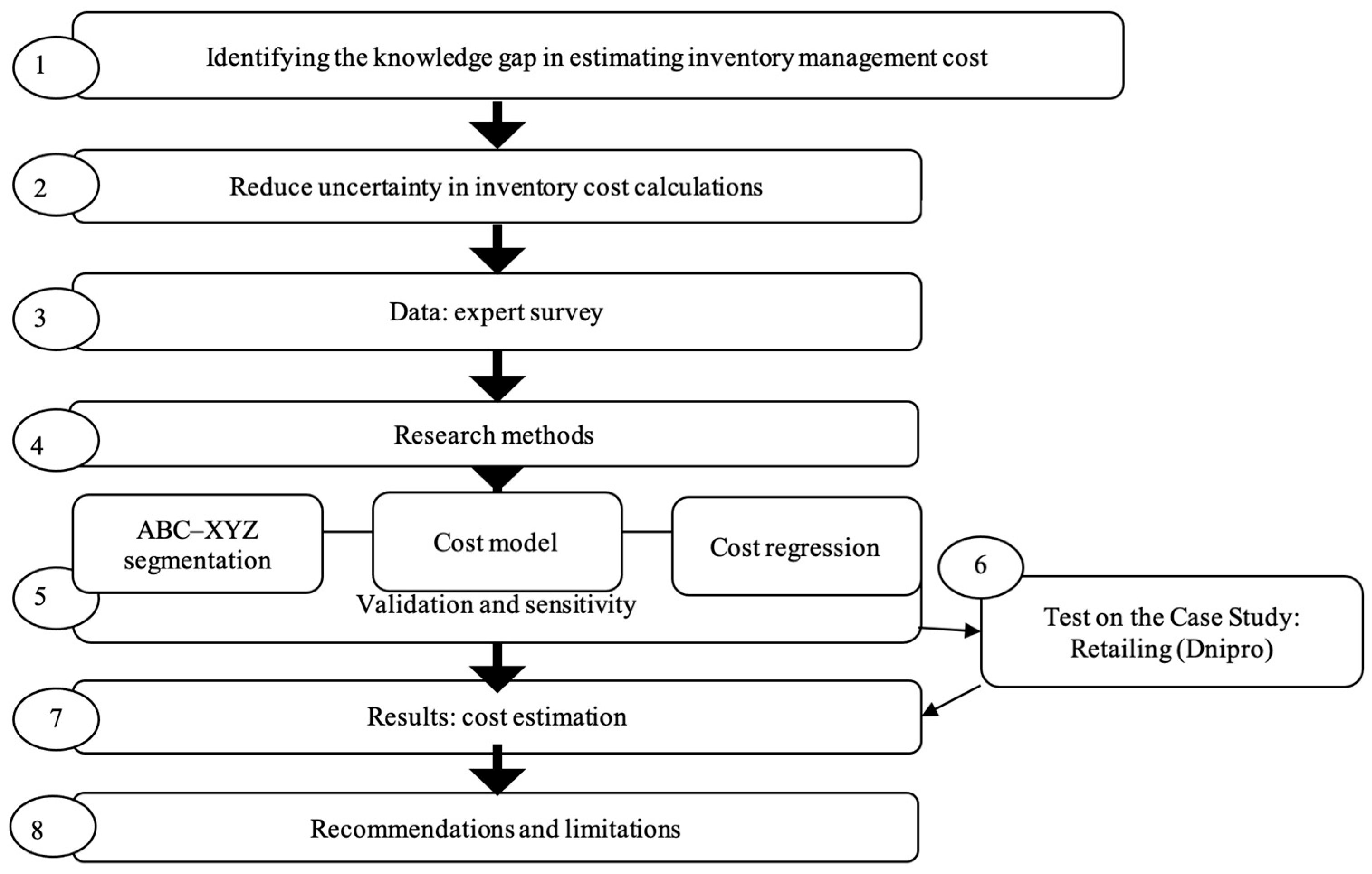
This section formalizes the logical structure of the study to address the existing knowledge gap regarding inventory management costing. The study includes seven stages (Figure 1).

Stage 1. Statement of the problem and aim. The study is based on the empirically observed decline in the resilience of small batch cargo (SBC) supply chains in times of crisis (economic problems, COVID-19, armed conflicts). The scientific problem is the uncertainty in calculating the costs of inventory management in retail logistics during failures. The aim is to develop and evaluate an applied methodological outline that reduces this uncertainty.

Stage 2. Data and identification of factors. To substantiate cost factors and evaluate the performance of models, a primary data set was collected based on expert opinion: a survey of sales agents in two cities (Dnipro, Ukraine; Almaty, Kazakhstan) on a 5-point Likert scale. The responses are normalized and aggregated to indicators used as criteria for segmentation in subsequent models for determining inventory management costs (deterministic and regression).

Stage 3. Methodological core (three methods).

(a)

Updated ABC-XYZ analysis. A product segmentation structure is proposed, supplemented by demand/supply stability criteria; the criteria serve as formal rules for assigning positions to classes and set management modes for each segment.

(b)

Additive cost model of inventory management. The total cost function is constructed as the sum of four components: warehouse maintenance, inventory maintenance (including the cost of capital), warehouse operations and capital immobilization. The model allows parameterization for various scenarios of failures occurring during the delivery process.

(c)

Regression model of operational forecast. A model of the dependence of the total costs of inventory management on the number of end customers, unit price and batch size are estimated. At the same time, regression coefficients show how costs can change with a slight change in each management parameter.

Stage 4. Validation and sensitivity analysis. The accuracy of the models is assessed by RMSE; sensitive analysis is carried out on key predictors and cost parameters. For interpretation, characteristic graphs are constructed to demonstrate the stability of the conclusions when factors vary.

Stage 5. Results and management conclusions. At the ABC-XYZ segment level, differentiated replenishment/insurance policies are set: at the cost level—quantitative guidelines for choosing storage and processing modes, and at the regression level—express estimates of costs when demand, price, and batch size change.

Stage 6. Applied verification (case study). The methodological framework is tested on data from retail companies (super/hypermarkets and distribution warehouses) for two sample cities. A comparison of predicted and actual costs, as well as scenario analysis of failures, confirm the applicability of the proposed approach for rapid decision making.

Stage 7. Limitations and limits of applicability. Limitations in geography and data sources (expert survey), as well as the dependence of the results on the parameters of the cost model are noted; directions for expansion are outlined (wider sampling, alternative loss functions, robust regression specifications).

Thus, the presented research framework provides end-to-end traceability from the problem to solutions and accuracy metrics and provides a basis for formally justifying segmentation.

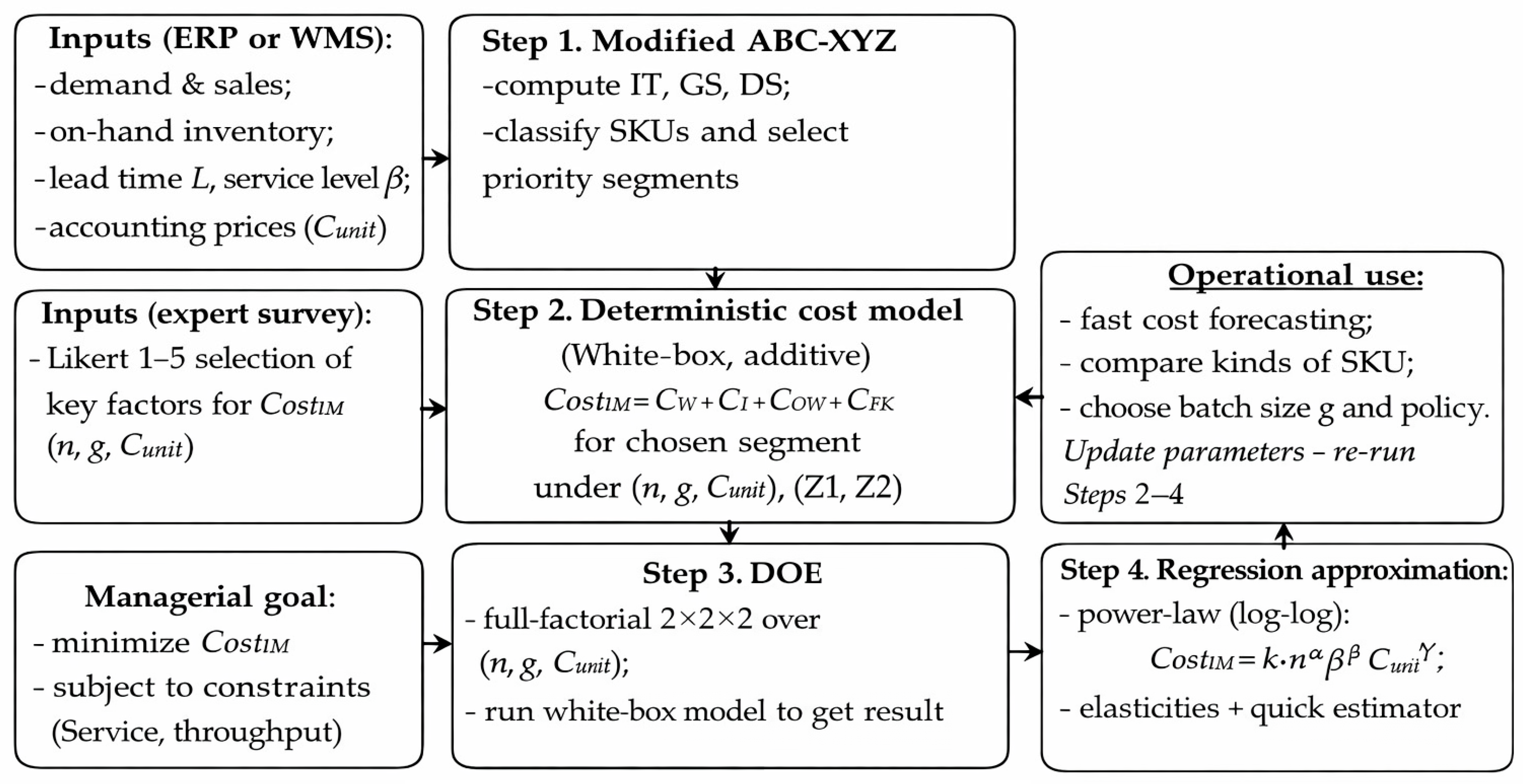
Figure 2 outlines the interaction of the three methodological blocks. Enterprise resource Planning (ERP) or Warehouse Management System (WMS) data are utilized in the modified ABC-XYZ procedure to compute inventory turnover (IT); goods significance (GS); and demand sustainability (DS), classify SKUs, and identify priority segments for intervention (e.g., Cost_IM). For these segments, the deterministic additive model assesses Cost_IM based on cost components and process parameters (n, g, C_unit, Z1, Z2). A full-factorial 2 × 2 × 2 design (Design of Experiments (DOE)) generates model responses for calibrating a power-law regression, allowing for quick what-if analyses when the operating conditions change, with updates to parameters and re-running of Steps 2–4.

3.3. Likert Scale to Define Key Variables

To select the factors that most influence inventory management costs, an expert survey of sales agents of two retail chains in large cities was conducted on a 5-point Likert scale (1—“minimal influence”, 5—“strong influence”) with open comments. The survey was conducted simultaneously in two locations—Almaty (Kazakhstan) and Dnipro (Ukraine)—over two consecutive weeks. Collection was carried out on weekdays, with batches divided into morning and evening shifts to minimize operational disruption in the warehouse and retail outlets.

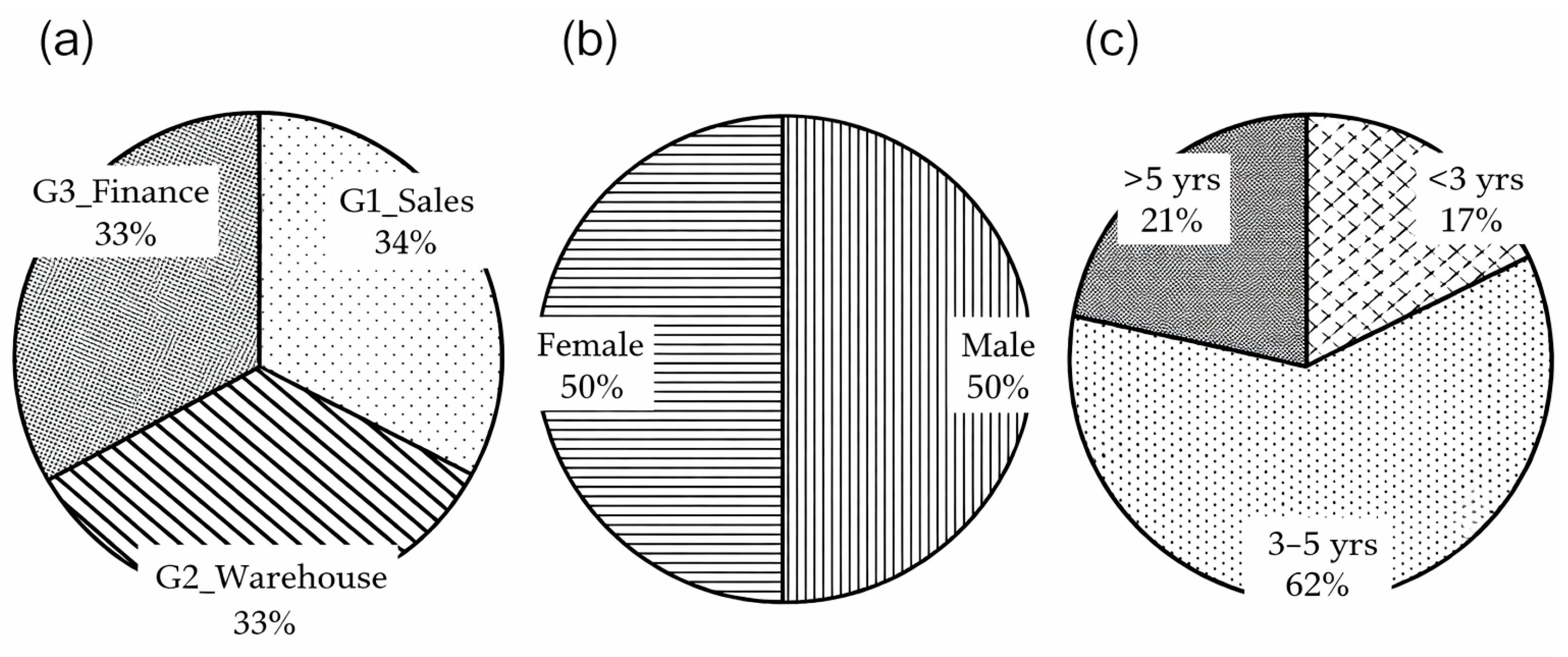
The sample included 24 experts: 12 from Almaty and 12 from Dnipro. Respondents are divided into three roles, corresponding to the research frame: G1_Sales—field sales agents/merchandisers (source of information about the frequency and size of orders, demand profile); G2_Warehouse—shift supervisors and warehouse operators (replenishment modes, productivity, organizational restrictions); and G3_Finance—specialists in financial controlling/inventory accounting (unit cost, immobilization rates, transaction rates). The selection of experts considered their distribution using groups (Figure 3a), the gender component (Figure 3b), and work experience (Figure 3c).

Purposive sampling was conducted based on at least 12 months of experience in the position, involvement in inventory/order planning, and regular work with the corporate accounting system/warehouse module. The criteria correspond to the recommendations for the formation of expert panels [76,77].

The expert survey included a mixed format: short face-to-face sessions in warehouses or offices and online questionnaires (personal links). The average filling time is 8–12 min. Expert identifiers were coded (E01–E24), and contact information was left voluntarily, solely for verification purposes.

Participants were presented with an information note about the purpose of the study; consent was confirmed by a mark in the questionnaire (Appendix A) and also supplemented by the results of the questionnaire (Appendix B). Responses were processed anonymously and published only in aggregate form (by city and expert group) (

Table 3. Likert selection matrix (medians by city and expert group).

Variable	Median/SD					Selection Result
	Almaty	Dnipro	G1	G2	G3
Replenishment batch size, g	4.0/0.669	4.0/0.515	4.0/0.463	4.5/0.744	4.0/0.641	Yes
Number of end customers, n	4.0/0.389	4.5/0.522	4.0/0.518	4.0/0.463	4.0/0.518	Yes
Average unit price, Cunit	4.0/0.793	4.0/0.669	4.0/0.835	4.0/0.518	3.5/0.535	Yes
Delivery time, L	3.0/0.996	4.0/0.515	3.5/0.744	3.5/0.886	3.5/0.744	No
Target service level, β	3.0/0.793	3.0/0.793	3.0/0.641	3.0/0.916	3.0/0.707	No
Mechanization performance, Z1	3.5/0.866	4.0/0.793	3.0/0.835	4.0/0.916	4.0/0.756	No
Cost of machine hour/operations, Z2	3.5/0.900	3.0/1.055	3.0/0.916	3.5/0.886	3.0/1.188	No

Note: Median—median of the score, and SD—standard deviation.

).

The questionnaire assessed seven factors (Table 3), formed based on the research design (Figure 1). For uniformity of understanding, brief definitions of the variables were given before the block of assessments. Scores were normalized to a range from [0, 1] and aggregated by the median. Next, the following selection filter was applied: median ≥0.7 and interquartile range ≤ 0.5 (IQR consensus criterion). The specified filter range was equivalent to the threshold’s median ≥3.5 and IQR ≤ 1, for a scale of 1–5 [78,79,80]. Based on the selection results, both models (deterministic and regression) included three controlled variables: batch size g, number of customers n, and unit price, C_unit. In addition to the median-and-IQR screening rule, we assessed inter-expert agreement by using the individual Likert ratings (Appendix B). Kendall’s coefficient of concordance indicates statistically significant agreement on the relative importance of the seven candidate factors (W = 0.331, χ²(6) = 47.59, p < 1 × 10⁻⁷). The average measures intraclass correlation for absolute agreement (ICC(2,k), two-way random effects) equals 0.911, confirming the good reliability of the aggregated expert judgment reported in Table 3.

The balance of cities (12 to 12, experts surveyed) and roles (G1; G2; G3) provides the full coverage and objectivity that is necessary to interpret the assessment of the total costs of inventory management.

In the next Section, Section 3.4, the choice of new criteria for ABC-XYZ analysis will be justified and their strict definitions will be given.

3.4. Justification of New Criteria for ABC-XYZ Analysis and Its Definitions

In this study, at the first stage, the selection of the most important groups of goods is proposed for the subsequent calculation of the costs of maintaining their inventories using a modified ABC-XYZ analysis. The use of a modified ABC-XYZ system provides proactively identifying product groups that require inventory, considering the following criteria:

• Inventory turnover, IT. Turnover is a key operating metric that reflects how many times inventory is sold or replaced during a period. Higher turnover indicates efficient use of finances and reduced storage costs. Empirical research demonstrates the relationship between turnover and corporate profitability—for example, in the Saudi Arabian manufacturing sector, higher inventory turnover is statistically associated with increased corporate profitability [81].
• Goods significance, GS. The significance goes beyond monetary value, given the critical importance of the product to logistics operations, branding and regulatory compliance. Modern methods for assessing the component and product criticality are also being developed—for example, a method for assessing component criticality that is consistent with the industry standard VDI 4800 Part 2 has recently been proposed [82].
• Demand sustainability, DS. Demand sustainability is usually assessed through the coefficient of variation (CV): a low CV corresponds to stable demand (category X), and a high CV usually corresponds to unstable demand (category Z). Recent research shows that forecasting methods, including deep learning, significantly improve forecast accuracy and optimize inventory management [83,84].

Thus, the combination of these three criteria forms a multidimensional ABC-XYZ matrix that aligns inventory management with both operational efficiency and strategic priorities. Thus, category AX (high turnover, strategic importance, stable demand) requires strict control and minimal inventory, while CZ (low turnover, low importance, unstable demand) can be serviced upon demand or be removed from the range (

Table 4. Resulting table of criteria justification for ABC-XYZ analysis.

Criterion	Description	Supporting Research
Inventory turnover, IT	The frequency of inventory sold or replaced indicates how efficiently operations are running.	[54,69,85,86]
Goods significance, GS	The importance of an item to operations goes beyond its monetary value; it includes factors such as regulatory requirements, brand significance, and the necessity of core inputs.	[5,87]
Demand sustainability, DS	Demand predictability can be classified based on variability: low, moderate, or high. This can be analyzed by using coefficient of variation (CV) analysis.	[85,88,89,90]

).

Moreover, innovative modeling and optimization techniques, such as system dynamics modeling with Bayesian optimization and differential evolutionary (DE) search methods, demonstrate significant improvements in profitability and reduction in costs through accurate modeling of demand and turnover dynamics [85,86].

Based on the selected criteria, the updated version of the ABC-XYZ analysis can be presented in

Table 5. Classification of enterprise inventories according to the criteria of turnover, significance and stability of demand (modified ABC-XYZ analysis).

	A	B	C
X	AX High Inventory Turnover, HIT; Strategic Goods Significance, SGS; Sustainable Demand, SD	BX Average Inventory Turnover, Tactical Goods Significance, Sustainable Demand	CX Low Inventory Turnover, Insignificance, Sustainable Demand
Y	AY High Inventory Turnover; Strategic Goods Significance; Demand Fluctuations	BY Average Inventory Turnover, Tactical Goods Significance, Demand Fluctuations	CY Low Inventory Turnover, Insignificance, Demand Fluctuations
Z	AZ High Inventory Turnover; Strategic Goods Significance; Unsustainable Demand	BZ Average Inventory Turnover, Tactical Goods Significance, Unsustainable Demand	CZ Low Inventory Turnover, Insignificance, Unsustainable Demand

.

Considering the above justifications in our study, we will use the following definitions according to the criteria used for the modified ABC-XYZ analysis assessment:

• Inventory turnover—The frequency of goods turnover in the warehouse (high, medium, low).
• Goods significance—The role of the product in overall activity, i.e., enterprise development strategies by product groups (strategic, tactical, insignificance).
• Demand sustainability—How uniformly and predictably the product is sold (sustainable, with fluctuations, or unsustainable).

Unlike classical ABC-XYZ, based only on sales value and demand variability, the modified procedure introduces inventory turnover and goods significance, fixes class boundaries via percentile-based IT cutoffs and cumulative-share rules for GS, and uses CV thresholds for DS to yield reproducible SKU-to-cell assignments (AX…CZ) and priority sets for subsequent costing and forecasting.

For each SKU i observed over 12 months, the inventory turnover ($I{T}_i$) is computed as follows:

$$I{T}_i={\displaystyle \frac{D}{{\overline{I}}_i,}}$$

(2)

where $D$ is annual demand (units) and ${\overline{I}}_i$ is average on-hand inventory (units) over the same period.

We classify turnover as high (HIT) if $I{T}_i\ge P_{67}(IT)$, medium if $P_{33}(IT)\le I{T}_i<P_{67}(IT)$, and low (LIT) if $I{T}_i<P_{33}(IT)$, where $P_{33}$ and $P_{67}$ are the 33rd and 67th percentiles across all SKUs in the case study (N = 46).

Goods significance (GS) is quantified by the annual sales value (ASV_i):

$$AS{V}_i=D_i\cdot C_{uni{t}_i}$$

(3)

In this study, SKUs are ranked by $ASV$, and classes ABC are formed by cumulative-share rules: A covers the smallest set of SKUs, accounting for the first 80% of cumulative $ASV$; B the next 15%; and C the remaining 5%. Hence, in the study, A-items are interpreted as “strategic”, B-items as “tactical”, and C-items as “insignificant”, reflecting their relative contribution to the annual sales.

Demand sustainability (DS) is measured by the coefficient of variation (CV_i) of monthly demand:

$$C{V}_i={\displaystyle \frac{\sigma (D_{i,m})}{\mu (D_{i,m})}},m=\mathrm{1...12},$$

(4)

In the study, DS assigns X (sustainable) if $C{V}_i\le 0.5$, Y (with fluctuations) if $0.5<C{V}_i\le 1$, and Z (unsustainable) if $C{V}_i>1$. Using these rules, each SKU is mapped to one cell (AX…CZ) in Table 5, and the resulting case study allocation is presented in

Table 6. Ranking of goods inventories, according to the level of importance and stability of demand.

	Group A	Group B	Group C
Group X	Shashlik ketchup Paprika sauce Special table margarine Premium Lviv mayonnaise Soy sauce Homemade mayonnaise for children Mild ketchup Special Sunny margarine Satsibeli sauce	Margarine Puff pastry for home baking Berry sauce	Hot homemade mustard Batumi sauce Grill sauce Steak ketchup Mango–chili sauce Mango–apricot mustard Sweet and sour sauce
Group Y	Provençal mayonnaise Salad mayonnaise Premium mayonnaise Light mayonnaise Cheese sauce Ukrainian sauce Golden mayonnaise Cheddar sauce Homemade margarine Margarine for baking Vermicelli chicken flavor Special milk margarine French mustard Sweet chili sauce Margarine Sloyka	Adjika sauce Honey mustard Chili ketchup Barbecue sauce Special cream margarine Lenten mayonnaise Curry sauce Special cream margarine Barbecue ketchup	Bloody Mary ketchup Burger sauce
Group Z	-	Kebab sauce Tartar sauce	-

.

The proposed criteria enable the selection of the most important groups of goods for which inventory holding costs can be incurred, using two alternative approaches: a deterministic approach (Section 3.3) and the nonlinear regression model (Section 3.4).

3.5. A Deterministic Approach for Inventory Cost Assessment

In this section, we develop an interpretable (“white”) deterministic model of the total cost of inventory management. While the cost structure is fixed, the model remains dynamic, allowing for re-parameterization when the external conditions change. This enables stress testing through targeted adjustments, such as labor-rate changes or capacity loss, in line with the paper’s scenario-oriented verification logic. The model serves as the initial response function for subsequent regression analysis (see Section 3.4), representing the final costs as the sum of the four observable components of the warehouse system and formulating the problem as minimization over controlled inputs.

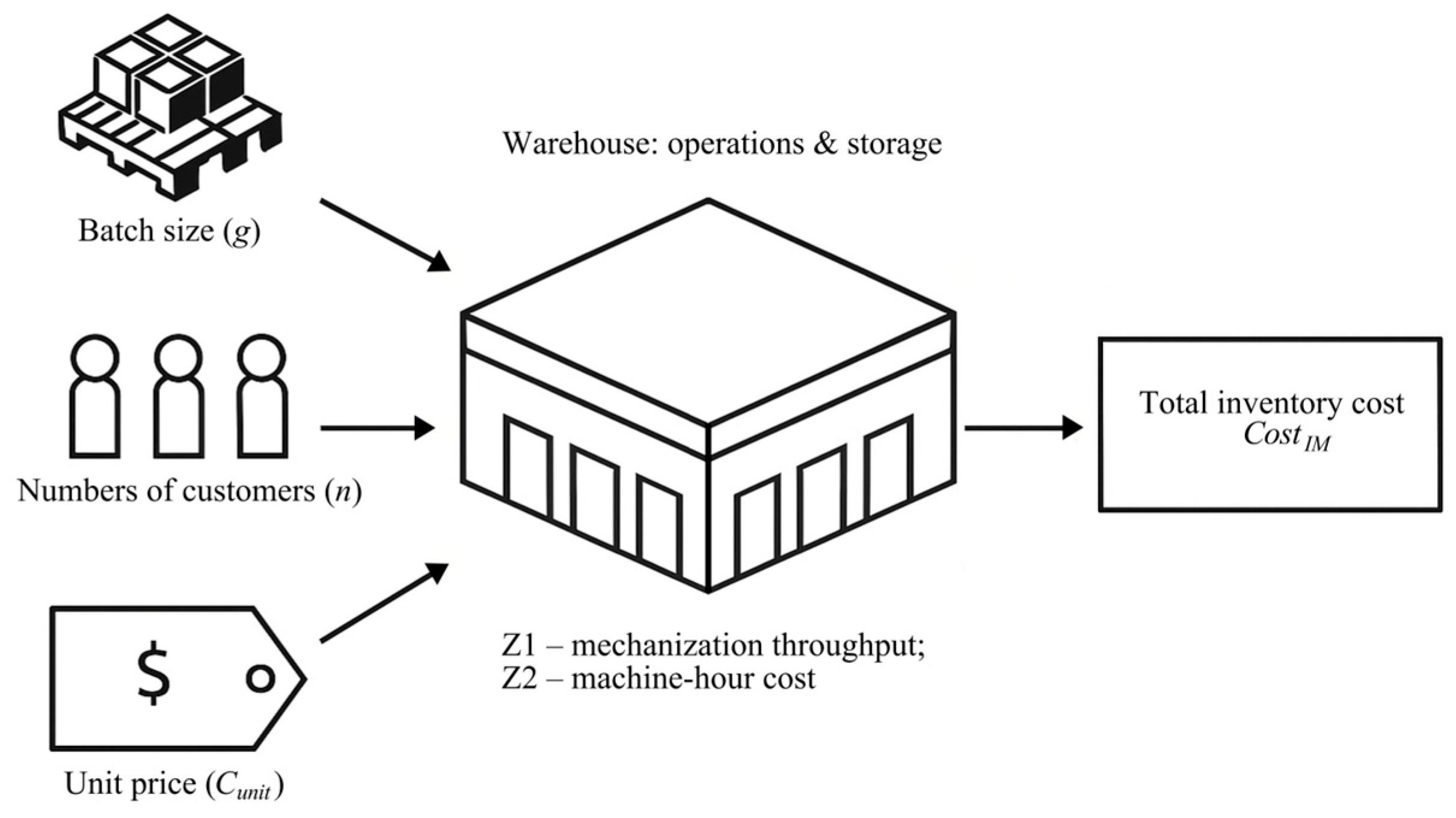
Visualization of the additive white box model shows how controlled inputs—batch size g, number of customers n and price per unit C_unit—through warehouse processes (operations and storage at given Z1, Z2) form the final cost Cost_IM (Figure 4). This deterministic scheme serves as a response function for further regression approximation of costs and analysis of parameter elasticities

In this case, in general, the target function of inventory management costs will look like this:

$$F_1:\min {\displaystyle \sum _{i\in G_p}{\displaystyle \sum _{k\in O_p}{\displaystyle \sum _{l\in P_p}Cos{t}_{I{M}_{ikl}}}}}\Rightarrow \min {\displaystyle \sum _{i\in G_p}{\displaystyle \sum _{k\in O_p}{\displaystyle \sum _{l\in P_p}(C_{W_{ikl}}}}}+C_{I_{ikl}}+C_{O{W}_{ikl}}+C_{F{K}_{ikl}}),$$

(5)

Taking into account the fact that the costs of warehouse work $C_{O{W}_{ikl}}$ consist of several cost items (for loading and unloading operations ($C_{U/L_{ikl}}$), moving ($C_{M{C}_{ikl}}$) and sorting of cargo in the warehouse ($C_{S{C}_{ikl}}$)), the target function will be expanded to the following form:

$$F_1:\min {\displaystyle \sum _{i\in G_p}{\displaystyle \sum _{k\in O_p}{\displaystyle \sum _{l\in P_p}(C_{W_{ikl}}}}}+C_{I_{ikl}}+C_{U/L_{ikl}}+C_{M{C}_{ikl}}+C_{S{C}_{ikl}}+C_{F{K}_{ikl}}),$$

(6)

Subject to the following:

$${\displaystyle \sum _{i\in G_p}{g}_i\le Q,\forall i\in G_p}$$

$${\displaystyle \sum _{k\in Q_p}{n}_{ki}\le N_{py},\forall i\in G_p},y=\{1;24\}$$

$${\displaystyle \sum _{l\in {{\rm P}}_p}{C_{unit}}_{li}\le C_p^w,\forall i\in G_p},\forall l\in {{\rm P}}_p$$

$$g_i\ge 0,\forall i\in G_p$$

$$n\ge 0$$

$${C_{unit}}_{li}\ge 0,\forall i\in G_p,\forall l\in {{\rm P}}_p$$

$$\gamma \le 1,\gamma \in \{0;1\},$$

$$I_{\min }\ge S_{ins} dueto{S}_{ins}=t_{\beta }\cdot \sigma$$

$$C_{M{C}_{ikl}}=C_{S{C}_{ikl}}$$

Since the inventory management model is presented in the form of a cybernetic white box model, the study was analytical, i.e., using mathematical formulas; each of the cost components of the objective function was determined $Cos{t}_{I{M}_{ikl}}$. In this case, the final additive model is presented, according to the following aggregate formula.

$$\begin{array}{l}Cos{t}_{IM}=C_1\cdot 365\cdot {\displaystyle \frac{g\cdot n\cdot \gamma }{N_{up}}}+D+C_{stor}\cdot t_p\cdot ({\displaystyle \frac{1}{2}}+{\displaystyle \frac{S_{ins}}{g\cdot n\cdot \gamma }})+{\displaystyle \frac{S_{up/un}\cdot n\cdot g\cdot \gamma \cdot (t_{1up}+t_{1un})}{n\cdot g\cdot \gamma }}+2\cdot {\displaystyle \frac{C_{man}\cdot T_{man}\cdot \eta \cdot g\cdot n\cdot \gamma }{g\cdot n\cdot \gamma }}+\\ +{\displaystyle \frac{C_{unit}\cdot N_d}{36500}}\cdot t_n\cdot ({\displaystyle \frac{1}{2}}+{\displaystyle \frac{S_{ins}}{g\cdot n\cdot \gamma }})\end{array}$$

(7)

Formula (7) was used to model inventory management costs when varying three variables ($g$,$n$,$C_{unit}$), which were identified by experts as the most significant (see Section 3.3).

3.6. Regression Model for Inventory Cost Assessment

In this section, we approximate the total cost of inventory management based on three control variables—g, n, and C_unit—which is justified in Section 3.3.

The study examined two competing hypotheses:

H1. 

A linear model describes inventory management costs better than nonlinear regression:

$$Cos{t}_{IM}={\beta }_0+{\beta }_1\cdot n+{\beta }_2\cdot g+{\beta }_3\cdot C_{unit}+\epsilon$$

(8)

where ${\beta }_i$ stands for linear regression model coefficients and $\epsilon$ stands for random error (perturbation, error term) in a regression model.

H2. 

A nonlinear model (logarithmic, power law) better describes inventory management costs than linear regression:

$$\ln (Cos{t}_{IM})=a_0+a_1\ln n+a_2\ln g+a_3\ln C_{unit}+\epsilon$$

(9)

where the coefficients $a_j$ are interpreted as elasticities, and the natural form of regression is restored as $Cos{t}_{IM}=A{n}^{a_1}{g}^{a_2}{C_{unit}}^{a_3}$.

From a theoretical perspective, Equation (9) represents a constant-elasticity cost function, which is generally used to describe how operational costs scale with activity and size variables. In small-batch warehousing, the dominant costs are activity-based (e.g., handling, picking) and combine a fixed setup with a variable workload. This typically results in sublinear cost growth, due to batching and resource pooling effects. The power-law form is used not only for statistical fitting but also for its interpretable elasticities and as a compact approximation for deterministic cost calculations in what-if analyses.

Since two levels of factor variation were chosen (minimum and maximum), and there are three factors themselves in the primary models, then according to the rules for constructing a full-factorial experimental design, it is necessary to conduct a 2 × 2 × 2 = 8 series of experiments. This two-level full-factorial design estimates first-order elasticities within the observed ranges. Expanding to three levels (3³ = 27) would address curvature effects but requires more empirical observations, which exceeds this single-case validation’s scope.

The evaluation of the constructed regressions was carried out using the least squares method (for a nonlinear model—after logarithm), followed by checking: (a) information content and signs of the coefficients; (b) goodness of fit, according to R², RMSE and information criteria (AIC/BIC); and (c) validity of residuals (tests for heteroskedasticity and normality), absence of multicollinearity (VIF) and stability of estimates in cross-validation (hold-out or cross-validation).

In the small calibration design (m = 8), predictive accuracy is evaluated using leave-one-out cross-validation (LOOCV). One design point is excluded per fold, the regression is re-estimated on the remaining points, and the excluded Cost_IM value is predicted. Performance is reported using RMSE(CV), MAE(CV), MAPE(CV), and the cross-validated coefficient (Q²).

$$Q^2=1-{\displaystyle \frac{PRESS}{TSS}}$$

(10)

where $PRESS$ is the sum of squared LOOCV prediction errors and $TSS$ is the total sum of squares around the sample mean.

4. Results and Validation

This section presents empirical results and verification of the methodology described in Section 3: (I) segmentation of the assortment using improved ABC-XYZ analysis, (II) estimation of the total costs of inventory management with a deterministic “white” model, (III) construction and comparison of regression specifications, (IV) characteristic bands for interpreting the influence of key factors and (V) applied conclusions for retail logistics small batch cargo deliveries. All calculations are reproducible and refer to the original tables and Appendix A, Appendix B, Appendix C and Appendix D of the manuscript.

4.1. Case Study

The case study was conducted at the warehouse of the trading company LLC “Schedro” (Dnipro, Ukraine). For representativeness, 46 SKUs (stock keeping units) were selected in the product subcategories of sauces/ketchups/margarines and related items that are typical for small batch cargo shipments. The observation base covered 12 consecutive months of 2023 (operational and price indicators for warehouses and retail outlets; Appendix C). These data served as the source of the demand and cost aggregates needed for subsequent calculations.

4.2. Results of the Modified ABC-XYZ Analysis

At the first step, the assortment is grouped using a modified ABC-XYZ analysis, which takes turnover, the importance of the product and the predictability of demand into account. Segments with high/medium business priority (AX, AY, AZ, BX, BY, BZ) are identified as basic ones for calculating costs—it is for them that it is advisable to maintain inventory and make tactical decisions on replenishment. The final ranking matrix is shown in Table 6. The assignment of SKUs to AX…CZ in Table 6 adheres to the quantitative rules for IT, ASV, and CV defined in Section 3.4, which include percentile-based IT cutoffs; 80, 15 and 5 ASV shares; and CV thresholds for XYZ.

4.3. Results of Estimating Inventory Management Costs

At the next stage, the cost of inventory management was calculated using Equation (7) for various combinations of variables. Calculations are made for cargo volumes that have the greatest weight in achieving the strategic goals of the enterprise, namely for goods with high and medium levels of demand. These are products belonging to groups AX, AY, AZ, BX, BY and BZ.

Therefore, for a comparable cost assessment, a full-factorial experimental design was formed: 2 × 2 × 2 for three controlled variables selected by experts (Section 3.3), which were the number of end customers n, [unit], the size of batch replenishment g, [ton], and the average unit price C_unit, [UAH/unit]. The following ranges of variable variation were used in the calculations: n ∈ {100;1000}, g ∈ {1.5;5}, and C_unit ∈ {30;150}. These data were obtained based on the results of monitoring in the retail trading network in the city of Dnipro. The 2 × 2 × 2 plan (m = 8) is a complete two-level full-factorial design for the three chosen inputs (n, g, C_unit), covering all corner combinations within their ranges. Expanding to three levels would require 27 runs and additional observations, which exceeds the scope of this single-case calibration. When conducting calculations, the following algorithm of actions is used.

For each SKU segment, cost components are calculated (warehouse maintenance, inventory maintenance, warehouse operations, capital immobilization) according to the deterministic function (Section 3.5).

The components are aggregated into the total cost Cost_IM for a given triple (n, g, C_unit).

Using a sample of eight combinations of parameters, the following are formed: (a) reference values of Cost_IM (

Table 7. Results of a full-factorial experiment.

Series of Experiments	Controlled Variables			Results of Calculating Costs for Inventory Management, UAH.
	n	g	Cunit
1	100	1.5	30	1727.16
2	1000	1.5	30	11,593.34
3	100	5	30	4222.80
4	1000	5	30	36,666.53
5	100	1.5	150	1799.72
6	1000	1.5	150	12,313.66
7	100	5	150	4244.52
8	1000	5	150	36,882.68

) and (b) training points for regression.

The results of calculations for eight series carried out as part of the experimental studies are presented in Table 7. This table is the “standard” for testing both deterministic and regression models.

4.4. Results of Regression Model Design and Validation

Using the MS Excel application package for m = 8, two regression models were developed and the hypotheses described in Section 3.6 were tested. The results of a comparison of two regressions are presented in

Table 8. Regression comparison.

Model	R2	Adj R2	RMSE	AIC	BIC	F	p(F)	m
Linear (levels)	0.837224	0.715142	5589.430692	168.76114	169.078906	6.857869	0.046896	8
Log–log (power)	0.996912	0.994596	1196.242237	−13.48836	−13.170603	430.471784	1.8 × 10−5	8

.

Based on Table 8, the nonlinear power model is convincingly better: higher R², much lower RMSE and information criteria (AIC and BIC), high F, and exceedingly small p(F). This confirms the hypothesis H2 and rejects the hypothesis H1 put forward in Section 3.6. The results of calculating the elasticity coefficients of the power regression model and their significance level are presented in

Table 9. Regression model (log–log): coefficients (elasticities).

Term	Estimate	StdErr	t	p-Value	CI Low (2.5%)	CI High (97.5%)
Intercept	2.927227	0.2366	12.37203	0.000245	2.270319	3.584135
ln(n)	0.88493	0.027433	32.257408	6 × 10−6	0.808763	0.961098
ln(g)	0.830684	0.052466	15.832782	9.3 × 10−5	0.685015	0.976353
ln(Cunit)	0.017466	0.039248	0.445002	0.679338	−0.091505	0.126436

.

Based on Table 8, it can be stated that the elasticities for n and g are positive and statistically significant. At the same time, the significance of C_unit at m = 8 is not confirmed, which is typical for small plans: 2 × 2 × 2. Alongside the limited power at m = 8, the near-zero elasticity of ln(C_unit) illustrates the SBC cost structure, where terms that are dependent on value are overshadowed by activity-based warehouses and operational costs within the examined price range.

The final form of the power regression model obtained from the case study results will be as follows:

$$CaseStudy:Cos{t}_{IM}=18.67n^{0.8849}{g}^{0.8307}$$

Further applied evaluations use nonlinear power-law regression as a more accurate and interpretable approximation of costs that are consistent with the “white” deterministic response function (Section 3.5).

To assess out-of-sample predictive accuracy, LOOCV was conducted on the full-factorial dataset (m = 8).

Table 10. Result of out-of-sample predictive accuracy of regression models (LOOCV, m = 8).

Model	RMSE(CV), UAH	MAE(CV), UAH	MAPE(CV), %	Q2 (LOOCV)
Linear (levels)	11,179	11,175	255.56	0.349
Log–log (power-law)	2336	1656	12.46	0.972

presents that the power-law model outperforms the linear model in predictive performance, with RMSE(CV) = 2336 UAH and MAPE(CV) = 12.46% compared to RMSE(CV) = 11,179 UAH and MAPE(CV) = 255.56%. The power-law model’s Q² value is 0.972, which is significantly higher than the linear model’s Q² = 0.349, indicating improved predictive capability. Fold-wise LOOCV predictions and percentage errors for each design point are available in Appendix D.

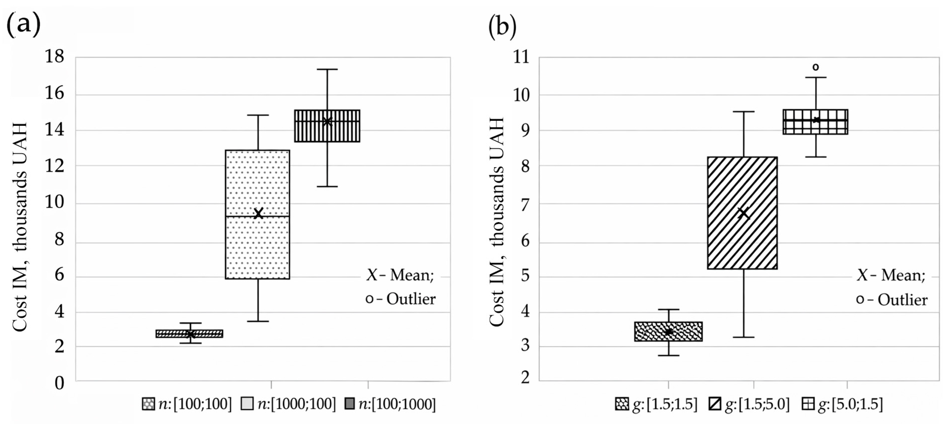
The greatest influence on costs is exerted by the customer’s quantity of cargo and the average size of batch cargo. The nature and degree of influence of the response function was determined based on the characteristic bands of the graph (Figure 5).

The bands in Figure 5a show that the predictions $Cos{t}_{IM}$ from the power-law regression model are distributed across three segments of n (the bottom, middle, and top third of observations). The median and interquartile range (Q1–Q3) increase monotonically from the lower to the upper segment, which confirms the positive and statistically significant elasticity, n. The number of outliers is small, and the antennae are of moderate length, which indicates the stability of the predictions in the operating range, n.

Similarly, the medians and Q1–Q3 increase with g in Figure 5b. This effect is comparable to the bands in Figure 5a and is consistent with the positive lng elasticity, which is determined by the positive values of the elasticity coefficients of the nonlinear regression model. The range of scatter widens slightly in the upper tertile, which reflects greater variability in costs for large batches and corresponds to a power-law (nonlinear) response shape.

Based on the analysis of the graph, it can be noted that the nature of the change in costs from changes in the values of indicators over the entire range of changes in indicators is constant. As each indicator increases, the costs of maintaining a warehouse also increase. The intensity of the change is also uniform over the entire range of changes in the indicator.

5. Discussion

This section discusses the empirical results obtained, their interpretation and the applicability of the proposed approach to calculating the total costs of inventory management in retail logistics small batch cargo deliveries, as well as limitations and comparison with alternative methods.

5.1. Key Findings

The proposed methodology is easily integrated into a real logistics system, due to a hybrid combination of the methods “modified ABC-XYZ–deterministic cost function–regression approximation”, which provides end-to-end traceability from strategic segmentation to operating costs, allowing for their operational forecasting (Table 6, Table 7 and Table 8, Figure 5).

Based on the Likert Scale, it was established that the key factors influencing the total costs of inventory management of the selected Cost_IM product segment are: the number of end customers, n; batch size, g; and unit cost, C_unit. However, according to the results of the regression analysis, the last factor (C_unit) within the studied range of values (case study) was found to be statistically insignificant. This fact is confirmed by the nonlinear power (log–log) model, which significantly exceeds the linear one in terms of the R², RMSE, AIC, BIC and F-criterion, confirming the hypothesis of the nonlinear nature of the dependence.

5.2. Discussion of Results

Firstly, the estimation algorithm proposed in our study (ABC-XYZ → “white” deterministic model → regression) eliminates the gap between the classification of inventories and the actual accounting of their holding costs. Selected segments of product groups, using a modernized ABC-XYZ analysis, determine the management modes, and the cost function makes these modes numerically comparable for specific variables (n, g, C_unit). A power-law regression model acts as a simple tool that determines the behavior of a warehouse logistics system, transforming a multi-step calculation into a simple power-law dependence.

In addition, when moving from the lower to the upper level of factors n and g, a strictly monotonic increase in total costs is observed (compare lines 1–4 and 5–8 in Table 7), which is consistent with the positive elasticities for lnn and lng in the adopted power-law regression model. Moreover, when varying C_unit within [30] with fixed n, g makes a relatively small contribution to the Cost_IM of a given warehouse (comparing pairs 1–5, 2–6, 3–7, 4–8), which explains the statistical insignificance ln C_unit in the sample m = 8 and the nature of small batch cargo logistics (the bulk of the costs are concentrated in the operational and warehouse part).

In SBC retail logistics, cost components are primarily activity-based (handling, picking, routing, etc.), scaling with service complexity and physical volume (represented by n and g), rather than inventory value. Within the proposed deterministic model, C_unit mainly impacts value-dependent items like capital immobilization and carrying costs, which are secondary for high or medium turnover segments. Table 7 highlights that a fivefold increase in C_unit (30 to 150 UAH/unit) results in only a slight change in Cost_IM at fixed n and g, unlike the significant changes from varying n or g. This demonstrates the practical insignificance of unit price in this SBC case.

It should be noted that the power regression model is more natural for warehouse systems. This aligns with constant-elasticity cost representations, in which sublinear exponents indicate the economies of scale and incomplete proportionality in operational resource use across the observed ranges. Furthermore, the choice of the power regression model is explained by the fact that the costs grow sublinearly for each factor (elasticity ≈ 0.88 for n and ≈0.83 for g), which reflects the effects of scale and the incomplete proportionality of resources. Thus, the final dependence can be interpreted according to the following rule: +1% to n or g provides =0.88% and =0.83% to Cost_IM, respectively.

5.3. Discussion on Feasibility of the Proposed Approach

From an implementation point of view, the proposed approach requires a minimum set of data:

• The average market operating tariffs and standard warehouse performance indicators for a deterministic model;
• The data on three controlled variables used as input factors (n, g, C_unit);
• Small experimental design (even 2 × 2 × 2) for calibration and verification of approximations.

In exchange, the organization receives a transparent calculation of the cost components, simple power regression for obtaining express forecasts, and visual tools (quartile bands) for quickly adjusting management decisions.

5.4. Limitations of the Proposed Approach

It should be noted that the proposed approach has a number of limitations.

Estimation is performed in a 2 × 2 × 2 design (m = 8), which limits the statistical power, especially for weak effects. To address the small-sample limitation, LOOCV predictive errors are reported (Table 10), with fold-wise diagnostics in Appendix D. Future work will focus on broader benchmarking with larger multi-warehouse datasets. The coefficient significance is interpreted with caution, primarily as an effect-screening indicator. The regression serves as a compact predictive model within the studied ranges, whereas transferring it to other contexts requires recalibration.

While the expert panel is moderate in size (n = 24) and shows stable aggregated judgments (Kendall’s W and ICC), future work should validate the screening with more firms and cities. The case base is one warehouse and a set of 46 SKUs, so transferring findings to other categories and regions requires additional calibration.

The deterministic model uses fixed rates and norms, which, in the case of external “shocks,” requires regular updating of parameters and, possibly, the use of robust modifications. In practical use, model parameters are considered as an updateable input vector, including labor rates, energy rates, handling tariffs, and penalty coefficients. Updates can be done either periodically, by recalculating rates from Enterprise Resource Planning or the Warehouse Management System and accounting records, or event-driven, by applying shock multipliers during disruptions and re-running the model. For broader applicability, the same workflow is used, but the parameter set is recalibrated to local market conditions.

In practice, n and g are partly jointly determined by service policies. Therefore, to eliminate bias, hierarchical models can be introduced.

5.5. Discussion of the Proposed Approach Comparability with Others

Compared to classical schemes (EOQ/EPQ [74,75] and target service-level approaches), the workflow preserves the interpretability of deterministic models and can be combined with the modified ABC-XYZ segmentation. In terms of predictive performance, the power-law approximation demonstrates improved out-of-sample accuracy, relative to the linear baseline under LOOCV (Table 10). Regarding implementation effort, the workflow relies on a small calibration design and standard spreadsheet-based estimation, whereas machine learning (ML) [13,33,48,69,70] and simulation approaches [21,23,51,67] typically require larger datasets, additional tuning, and specialized software. Therefore, the statement on lower implementation cost refers to data and tooling requirements; direct accuracy benchmarking against ML or simulation is outside the scope of the present dataset and is identified as future work on larger samples.

The practical implementation of the proposed approach will make it possible to establish a rational size of batch g, so that the increase in costs per unit of growth is minimal. On the other hand, client management in the context of the approach involves increasing n through the introduction of technological solutions (warehouse routing, slotting, time windows). Also, the manager should periodically review the SKU according to the modified ABC-XYZ, and synchronize the product replenishment policies based on identified cost items.

These managerial implications depend on the specific warehouse context and observed factors. While the workflow can be adapted to other warehouses or products, the cost parameters and regression coefficients must be recalibrated with local data before implementation.

6. Conclusions

This study proposes a new, repeatable methodology for quickly estimating the total inventory management costs of small batch cargo (SBC) deliveries under conditions of uncertainty. The approach is based on the sequential application of a modified ABC-XYZ analysis, a deterministic additive cost model and regression approximation, which establishes patterns for controlled inputs (number of customers n, batch size g, unit price Cunit) and the response function (total costs of inventory management Cost_IM). The approach is aimed at reducing uncertainty and increasing the sustainability of decisions at the warehouse and retail logistics level.

The study used the following methods: ABC-XYZ segmentation (for prioritizing positions), additive cost function (decomposition of costs into four components) and comparison of two regressions (linear and power) with subsequent diagnostics R², RMSE, AIC, BIC, and visual validation (construction of characteristic bands), as well as out-of-sample validation, using LOOCV predictive errors.

As a result of the comparison, the power regression model turned out to be the best (R² = 0.9969, RMSE = 1196, versus linear: R² = 0.8372, RMSE = 5589), which confirms the nonlinear nature of the response. The regression coefficients (elasticities) turned out to be statistically significant for n = 0.885 and g = 0.831, and for lnCunit, but insignificant in the sample m = 8 and in the studied range of inventory management costs. Visualization of characteristic bands by tertiles n and g shows a monotonic increase in the median in quartiles Q1–Q3, which is consistent with the signs of the coefficients. The main practical conclusion from the results is that +1% to n or g increases Cost_IM by approximately 0.88% and 0.83%, respectively. In this case, the estimated elasticities show sublinear cost scaling concerning n and g, with a weak effect of C_unit. These estimates are case-specific; however, the paper’s main contribution is the reproducible workflow that is applicable elsewhere after calibration.

Directions for further research include expanding the database (more SKUs, categories and locations), moving from a 2 × 2 × 2 design to a larger array of controlled factors, considering the possibility of using hierarchical models, and adding stochastic supply characteristics with the ability to test robust and Bayesian regressions. From a strategic perspective, improved and unified results can be integrated into a methodology with ML or simulations for stress testing scenarios and replenishment policies for segments AX, AY, and BX.

References

1. Ivanov, D.; Dolgui, A. A digital supply chain twin for managing disruption risks and resilience in the era of Industry 4.0. Prod. Plan. Control 2021, 32, 775–788. [Google Scholar] [CrossRef]
2. Taran, I.; Kairatkyzy, G.; Pavlenko, O.; Nefyodov, V.; Muzylyov, D. Determining the optimal service area of a logistics center: A quantitative approach. Transp. Probl. 2025, 20, 5–19. [Google Scholar] [CrossRef]
3. Mitręga, M.; Choi, T. How small- and medium transportation companies handle asymmetric customer relationships under COVID-19 pandemic. Transp. Res. Part E 2021, 148, 102249. [Google Scholar] [CrossRef] [PubMed]
4. Zhao, N.; Hong, J.; Lau, K.H. Impact of supply chain digitalization on supply chain resilience and performance: A multi-mediation model. Int. J. Prod. Econ. 2023, 259, 108817. [Google Scholar] [CrossRef] [PubMed]
5. Li, P.; Chen, Y.; Guo, X. Digital transformation and supply chain resilience. Int. Rev. Econ. Financ. 2025, 99, 104033. [Google Scholar] [CrossRef]
6. Queiroz, M.M.; Ivanov, D.; Dolgui, A.; Fosso Wamba, S. Impacts of epidemic outbreaks on supply chains: Mapping a research agenda amid the COVID-19 pandemic through a structured literature review. Ann. Oper. Res. 2022, 319, 1159–1196. [Google Scholar] [CrossRef] [PubMed]
7. Muzylyov, D.; Shramenko, N. Mathematical model of reverse loading advisability for trucks considering idle times. In New Technologies, Development and Application III; Karabegović, I., Ed.; Springer: Cham, Switzerland, 2020; pp. 612–620. [Google Scholar] [CrossRef]
8. Medvediev, I.; Muzylyov, D.; Shramenko, N.; Nosko, P.; Eliseyev, P.; Ivanov, V. Design logical linguistic models to calculate necessity in trucks during agricultural cargoes logistics using fuzzy logic. Acta Logist. 2020, 7, 155–166. [Google Scholar] [CrossRef]
9. Avinadav, T.; Chernonog, T.; Meilijson, I.; Perlman, Y. A consignment contract with revenue sharing between an app developer and a distribution platform. Int. J. Prod. Econ. 2021, 243, 108322. [Google Scholar] [CrossRef]
10. Ben Jeddou, M. Multi-criteria ABC inventory classification—A case of vehicles spare parts items. J. Adv. Manag. Sci. 2014, 2, 181–185. [Google Scholar] [CrossRef]
11. Venkatesh, D.P.; Sowmiya, M.P. ABC-XYZ classification and forecasting for inventory optimization. Int. J. Res. Publ. Rev. 2024, 5, 5348–5357. [Google Scholar] [CrossRef]
12. Aktepe, A.; Ersoz, S.; Turker, A.; Barisci, N.; Dalgic, A. An inventory classification approach combining expert systems, clustering, and fuzzy logic with the ABC method, and an application. S. Afr. J. Ind. Eng. 2018, 29, 49–62. [Google Scholar] [CrossRef]
13. Baratsas, S.; Iseri, F.; Pistikopoulos, E.N. A hybrid statistical and machine learning-based forecasting framework for the energy sector. Comput. Chem. Eng. 2024, 188, 108740. [Google Scholar] [CrossRef] [PubMed]
14. Ouamani, F.; Ben Fredj, A.; Fekih, M.R.; Msahli, A.; Ben Saoud, N.B. A hybrid model for demand forecasting based on the combination of statistical and machine learning methods. In International Conference on Advanced Data Mining and Applications; Springer: Cham, Switzerland, 2022. [Google Scholar] [CrossRef]
15. Boylan, J.; Syntetos, A. Intermittent Demand Forecasting: Context, Methods and Applications; John Wiley & Sons, Ltd.: Chichester, UK, 2021. [Google Scholar] [CrossRef]
16. Govindan, K.; Mina, H.; Alavi, B. A decision support system for demand management in healthcare supply chains considering epidemic outbreaks. Transp. Res. Part E Logist. Transp. Rev. 2020, 138, 101967. [Google Scholar] [CrossRef]
17. Lin, S.; Karia, N. Impact of digitalization on supply chain performance in the manufacturing industry: A literature review. Glob. Bus. Manag. Res. 2024, 16, 3746. [Google Scholar]
18. Golan, M.S.; Jernegan, L.H.; Linkov, I. Trends and applications of resilience analytics in supply chain modeling: Systematic literature review in the context of the COVID-19 pandemic. Environ. Syst. Decis. 2020, 40, 222–243. [Google Scholar] [CrossRef] [PubMed]
19. Sodhi, M.S.; Tang, C.S. Supply chain management for extreme conditions: Research opportunities. J. Supply Chain Manag. 2021, 57, 7–16. [Google Scholar] [CrossRef]
20. Wieland, A. Dancing the supply chain: Toward transformative supply chain management. J. Supply Chain Manag. 2021, 57, 58–73. [Google Scholar] [CrossRef]
21. Pavlenko, O.; Muzylyov, D.; Trojanowski, P. Finding a rational option for a cold supply chain using simulation on international routes. In Smart Technologies in Urban Engineering (STUE 2023); Springer: Cham, Switzerland, 2023; pp. 297–307. [Google Scholar] [CrossRef]
22. Shekarian, M.; Mellat Parast, M. An integrative approach to supply chain disruption risk and resilience management: A literature review. Int. J. Logist. Res. Appl. 2020, 24, 427–455. [Google Scholar] [CrossRef]
23. Zhanbirov, G.; Litvin, V.; Taran, I.; Izteleuova, M.; Aliakbarkyzy, D. Substantiation of a reasonable number of forklifts for a warehouse complex with frontal racks in an anylogic environment. Transp. Probl. 2023, 18, 147–160. [Google Scholar] [CrossRef]
24. Kreng, V.B.; Tan, S.-J. The optimal replenishment decisions under two levels of trade credit policy depending on the order quantity. Expert Syst. Appl. 2010, 37, 5514–5522. [Google Scholar] [CrossRef]
25. Jaber, M.Y.; Peltokorpi, J. Economic order/production quantity (EOQ/EPQ) models with product recovery: A review of mathematical modelling (1967–2022). Appl. Math. Model. 2024, 129, 655–672. [Google Scholar] [CrossRef]
26. Solari, F.; Lysova, N.; Bocelli, M.; Volpi, A.; Montanari, R. Perishable product inventory management in the case of discount policies and price-sensitive demand: Discrete time simulation and sensitivity analysis. Procedia Comput. Sci. 2024, 232, 1233–1241. [Google Scholar] [CrossRef]
27. Sá, S.; do Sameiro Carvalho, M.; Gonçalves, J.N.C. A decision support system to define new inventory management policies. Procedia Comput. Sci. 2025, 263, 25–33. [Google Scholar] [CrossRef]
28. Shramenko, V.; Shramenko, N.; Hupfer, C. Sustainable development of rural areas: Machine learning for semantic segmentation of agricultural fields. In Smart Cities: Importance of Management and Innovations for Sustainable Development; Mobility IoT 2023; EAI/Springer Innovations in Communication and Computing; Cagáňová, D., Cehlár, M., Horňáková, N., Eds.; Springer: Cham, Switzerland, 2024. [Google Scholar] [CrossRef]
29. Khan, M.S.R. The effects of inventory management capability on performance of the firm-Business strategies as a mediating role. Asian Financ. Bank. Rev. 2020, 4, 1–7. [Google Scholar] [CrossRef]
30. Kurniawan, S.; Saragih, M.H.; Angelina, V. Inventory control analysis with continuous review system and periodic review system methods at PT. XYZ. Business Economic. Commun. Soc. Sci. (BECOSS) J. 2022, 4, 97–109. [Google Scholar] [CrossRef]
31. Rizkya, I.; Syahputri, K.; Sari, R.M.; Anizar; Siregar, I.; Ginting, E. Comparison of periodic review policy and continuous review policy for the automotive industry inventory system. In IOP Conference Series: Materials Science and Engineering; IOP Publishing: Bristol, UK, 2018; Volume 288, p. 012085. [Google Scholar] [CrossRef]
32. Rahmadani, L.; Sagaf, M.; Syakhroni, A. Analysis of raw material inventory ABC classification using continuous review system and periodic review system methods to optimize production costs. J. Disprotek 2025, 16, 57–68. [Google Scholar] [CrossRef]
33. Behzad, A.; Pirayesh, M.; Ranjbar, M. Considering continuous review policy in a two-echelon inventory system using a reinforcement learning approach. Int. J. Procure. Manag. 2025, 23, 385–405. [Google Scholar] [CrossRef]
34. Lee, E.; Yuk, H.; Kim, S.Y. Marketing capability and firm performance: The mediating effects of market sensing capability and customer relationship management capability in the relationship between channel management capability and firm innovation. Korean J. Mark. 2023, 38, 19–44. [Google Scholar] [CrossRef]
35. Yosan, R.B.; Kholil, M.; Hanum, B. Implementation of inventory management system (IMS): Case study on XYZ online store. In IOP Conference Series: Materials Science and Engineering; IOP Publishing: Bristol, UK, 2018; Volume 343, p. 012022. [Google Scholar] [CrossRef]
36. Gonçalves, J.N.C.; Sameiro Carvalho, M.; Cortez, P. Operations research models and methods for safety stock determination: A review. Oper. Res. Perspect. 2020, 7, 100164. [Google Scholar] [CrossRef]
37. Albrecht, M. Optimization of safety stocks in models with an order service level objective or constraint. Eur. J. Oper. Res. 2017, 263, 900–909. [Google Scholar] [CrossRef]
38. Monek, G.D.; Fischer, S. IIoT-supported manufacturing-material-flow tracking in a DES-based digital-twin environment. Infrastructures 2023, 8, 75. [Google Scholar] [CrossRef]
39. Panchenko, A.; Prokhorchenko, A.; Panchenko, S.; Dekarchuk, O.; Gurin, D.; Medvediev, I. Predicting the estimated time of cargo dispatch from a marshaling yard. East. Eur. J. Enterp. Technol. 2020, 4, 6–15. [Google Scholar] [CrossRef]
40. Ren, Z. Literature review related to spare parts demand forecasting and inventory management. Econ. Bus. Manag. 2025, 1, 81. [Google Scholar] [CrossRef]
41. Bhalla, S.; Alfnes, E.; Hvolby, H.-H.; Sgarbossa, F. Advances in spare parts classification and forecasting for inventory control: A literature review. IFAC-Pap. 2021, 54, 982–987. [Google Scholar] [CrossRef]
42. Kulshrestha, N.; Agrawal, S.; Shree, D. Spare parts management in Industry 4.0 era: A literature review. J. Qual. Maint. Eng. 2024, 30, 248–283. [Google Scholar] [CrossRef]
43. Lolli, F.; Coruzzolo, A.M.; Peron, M.; Sgarbossa, F. Insourcing additive manufacturing for spare parts production: Is it profitable? Int. J. Prod. Res. 2024, 63, 3961–3981. [Google Scholar] [CrossRef]
44. Duarte, E.; de Haro Moraes, D.; Padula, L.L. An empirical study of learning-to-rank for spare parts consumption in the repair process. Expert Syst. 2023, 40, e13441. [Google Scholar] [CrossRef]
45. Setiawan, I.; Rasul, R.; Rusman, M. Analysis of product inventory control using continuous review system Q and periodic review system P to minimize inventory costs. J. Rekayasa Sist. Ind. 2023, 10, 47. [Google Scholar] [CrossRef]
46. Feng, L. Dynamic pricing, quality investment, and replenishment model for perishable items. Int. Trans. Oper. Res. 2018, 26, 1558–1575. [Google Scholar] [CrossRef]
47. Suwignjo, P.; Panjaitan, L.; Baihaqy, A.R.; Rusdiansyah, A. Predictive analytics to improve inventory performance: A case study of an FMCG company. Oper. Supply Chain Manag. Int. J. 2023, 16, 293–310. [Google Scholar] [CrossRef]
48. Walter, A.; Ahsan, K.; Rahman, S. Application of artificial intelligence in demand planning for supply chains: A systematic literature review. Int. J. Logist. Manag. 2025, 36, 672–719. [Google Scholar] [CrossRef]
49. Monek, G.D.; Fischer, S. Expert twin: A digital twin with an integrated fuzzy-based decision-making module. Decis. Mak. Appl. Manag. Eng. 2024, 8, 1–21. [Google Scholar] [CrossRef]
50. Fildes, R.; Goodwin, P.; De Baets, S. Forecast value added in demand planning. Int. J. Forecast. 2025, 41, 649–669. [Google Scholar] [CrossRef]
51. Kaščak, J.; Husár, J.; Knapčíková, L.; Trojanowska, J.; Ivanov, V. Conceptual Use of Augmented Reality in the Maintenance of Manufacturing Facilities. In Advances in Manufacturing III; Trojanowska, J., Kujawińska, A., Machado, J., Pavlenko, I., Eds.; MANUFACTURING 2022. Lecture Notes in Mechanical Engineering; Springer: Cham, Switzerland, 2022; pp. 241–252. [Google Scholar] [CrossRef]
52. Balkhi, B.; Alshahrani, A.; Khan, A. Just-in-time approach in healthcare inventory management: Does it really work? Saudi Pharm. J. 2022, 30, 1830–1835. [Google Scholar] [CrossRef]
53. Buń, P.; Trojanowska, J.; Ivanov, V.; Pavlenko, I. The Use of Virtual Reality Training Application to Increase the Effectiveness of Workshops in the Field of Lean Manufacturing. In Proceedings of the International Conference of the Virtual and Augmented Reality in Education; Bruzzone, A.G., Ginters, E., González Mendívil , E., Gutierrez, J.M., Longo, F., Eds.; DIMEG—University of Calabria: Genoa, Italy; Rende, Italy, 2018; pp. 65–69. [Google Scholar]
54. Gao, D.; Wang, N.; He, Z.; Zhou, L. Analysis of bullwhip effect and inventory cost in the online closed-loop supply chain. Int. J. Prod. Res. 2022, 61, 6808–6828. [Google Scholar] [CrossRef]
55. Das, S.C.; Akhtar, F.; Alrasheedi, A.F.; Shaikh, A.A. Application of water cycle algorithm with demand follows green level and nonlinear power pattern of the product for an inventory system. Sci. Rep. 2024, 14, 20995. [Google Scholar] [CrossRef]
56. Saputro, T.E.; Figueira, G.; Almada-Lobo, B. A comprehensive framework and literature review of supplier selection under different purchasing strategies. Comput. Ind. Eng. 2022, 167, 108010. [Google Scholar] [CrossRef]
57. Sakulsom, N.; Tharmmaphornphilas, W. Multi-mode replenishment strategies for periodic-review in 2-echelon systems under seasonal demand. J. Ind. Eng. Manag. 2024, 17, 562. [Google Scholar] [CrossRef]
58. Keshavarz-Ghorbani, F.; Pasandideh, S.H.R. A model of determining the ordering strategy for a multi-product problem with lateral transshipment approach: Hybrid metaheuristic algorithms. J. Ambient. Intell. Humaniz. Comput. 2022, 14, 6769–6782. [Google Scholar] [CrossRef]
59. Karakatsoulis, G.; Skouri, K. A periodic review inventory model facing different disruption profiles. Int. J. Prod. Econ. 2023, 265, 109004. [Google Scholar] [CrossRef]
60. Kusomrosananan, T.; Phumchusri, N. Inventory policy improvement with periodic review for perishable goods: A case study of a retail coffee shop in Thailand. Eng. J. 2024, 28, 59–73. [Google Scholar] [CrossRef]
61. Kalinichenko, O.; Pavlenko, O.; Medvediev, I.; Turpak, S.; Muzylyov, D. Updated Warehouse Logistics in Space-Constrained Environments Using Routing and Technical Solutions. In Intelligent Transport Systems: Ecology, Safety, Quality, Comfort. ITSESQC 2024; Slavinska, O., Danchuk, V., Kunytska, O., Hulchak, O., Eds.; Lecture Notes in Networks and Systems; Springer: Cham, Switzerland, 2025; Volume 1336, pp. 256–267. [Google Scholar] [CrossRef]
62. Suvetha, R.; Rangarajan, K.; Rajadurai, P. A sustainable three-stage production inventory model with trapezoidal demand and time-dependent holding cost. Results Control Optim. 2024, 17, 100493. [Google Scholar] [CrossRef]
63. Malicki, S.; Minner, S. The impact of initial inventory assumptions on cost performance in lot-sizing models. Eur. J. Oper. Res. 2025, 329, 447–459. [Google Scholar] [CrossRef]
64. Taran, I.; Litvin, V.; Zhanbirov, G. Optimisation of logistics processes in a warehouse complex equipped with gravity racking system using simulation modelling. In Proceedings of the 27th International Scientific Conference Transport Means 2023: Sustainability—Research and Solutions; Kaunas University of Technology: Kaunas, Lithuania, 2023; Part II; pp. 838–843. [Google Scholar] [CrossRef]
65. Alnahhal, M.; Aylak, B.L.; Al Hazza, M.; Sakhrieh, A. Economic order quantity: A state-of-the-art in the era of uncertain supply chains. Sustainability 2024, 16, 5965. [Google Scholar] [CrossRef]
66. Jadidi, O.; Firouzi, F.; Sorooshian, S. A closed-form solution approach for optimal reorder point in economic order quantity models with uncertain demands. Decis. Anal. J. 2025, 16, 100622. [Google Scholar] [CrossRef]
67. Tebaldi, L.; Bigliardi, B.; Filippelli, S.; Bottani, E. EOI or EOQ? A simulation study for the inventory management of a railway sector company. Procedia Comput. Sci. 2023, 217, 1532–1541. [Google Scholar] [CrossRef]
68. Taran, I.; Karsybayeva, A.; Naumov, V.; Murzabekova, K.; Chazhabayeva, M. Fuzzy-Logic Approach to Estimating the Fleet Efficiency of a Road Transport Company: A Case Study of Agricultural Products Deliveries in Kazakhstan. Sustainability 2023, 15, 4179. [Google Scholar] [CrossRef]
69. Seyedan, M.; Mafakheri, F.; Wang, C. Order-up-to-level inventory optimization model using time-series demand forecasting with ensemble deep learning. Supply Chain Anal. 2023, 3, 100024. [Google Scholar] [CrossRef]
70. Rizqi, Z.U.; Chou, S.-Y. Neuroevolution reinforcement learning for multi-echelon inventory optimization. Eng. Appl. Artif. Intell. 2024, 134, 108670. [Google Scholar] [CrossRef]
71. Siriruk, P.; Kotekangpoo, A. Order quantity optimization model for perishable products under continuous review (Q, r) with stochastic demand and positive lead time. Omega 2025, 138, 103392. [Google Scholar] [CrossRef]
72. Palanivel, M.; Venkadesh, M.; Vetriselvi, S.; Suganya, M. An analytics-driven EOQ model integrating fuzzy learning for deteriorating imperfect items. Supply Chain Anal. 2025, 10, 100120. [Google Scholar] [CrossRef]
73. Nguyen, T.N.A.; Nguyen, T.X.H.; Tran, N.T.; Nguyen, T.H.; Nguyen, P.A.; Vu, H.A. Optimizing supply chain operations using advanced time-series mixer models for demand forecasting and inventory under uncertain demand. Expert Syst. Appl. 2026, 296, 128955. [Google Scholar] [CrossRef]
74. Silver, E.A.; Pyke, D.F.; Peterson, R. Inventory Management and Production Planning and Scheduling, 3rd ed; John Wiley & Sons: New York, NY, USA, 1998. [Google Scholar]
75. King, P.L. Understanding Safety Stock and Mastering Its Equations. MIT Course Reading. 2014. Available online: https://web.mit.edu/2.810/www/files/readings/King_SafetyStock.pdf (accessed on 10 October 2025).
76. Ferrazzi, G.; Micai, M.; Fulceri, F.; Pingani, L.; Ghirotto, L.; Scattoni, M.L.; Galeazzi, G.M. From policy to practice: A Delphi protocol on life projects for autistic adults. Int. J. Qual. Methods 2025, 24, 16094069251357766. [Google Scholar] [CrossRef]
77. Medvediev, I.; Muzylyov, D.; Montewka, J. Human-centered method estimating safe width of inland waterways. Ocean Eng. 2026, 352, 124448. [Google Scholar] [CrossRef]
78. Wróbel, A.; Cash, P.; Maier, A.; Paulin Hansen, J. Determining the prioritization of behavior change techniques for long-term stroke rehabilitation: Delphi survey study. Interact. J. Med. Res. 2025, 14, e59172. [Google Scholar] [CrossRef]
79. Thoomes, E.; Falla, D.; Cleland, J.A.; Fernández-De-Las-Peñas, C.; Gallina, A.; de Graaf, M. Conservative management for lumbar radiculopathy based on the stage of the disorder: A Delphi study. Disabil. Rehabil. 2023, 45, 3539–3548. [Google Scholar] [CrossRef]
80. Price, J.; Rushton, A.; Tyros, V.; Heneghan, N.R. Consensus on the exercise and dosage variables of an exercise training programme for chronic non-specific neck pain: Protocol for an international e-Delphi study. BMJ Open 2020, 10, e037656. [Google Scholar] [CrossRef]
81. Alnaim, M.; Kouaib, A. Inventory turnover and firm profitability: A Saudi Arabian investigation. Processes 2023, 11, 716. [Google Scholar] [CrossRef]
82. Proff, S.; Heinemann, S.; Ritthoff, M. Assessment of product criticality at the corporate level presenting a newly developed method based on standard VDI 4800 Part 2. Clean. Logist. Supply Chain 2025, 16, 100241. [Google Scholar] [CrossRef]
83. Aldahmani, E.; Alzubi, A.; Iyiola, K. Demand forecasting in supply chain using uni-regression deep approximate forecasting model. Appl. Sci. 2024, 14, 8110. [Google Scholar] [CrossRef]
84. Rakholaia, K.R.; Chandraprabh, C.; Ramesh, R.; Rao, K.S.; Punitha, S.; Kumar, M.G.V. Optimizing Inventory Management through Demand Forecasting: A Data-Driven Approach for Enhanced Supply Chain Efficiency. SSRN Electron. J. 2025. [Google Scholar] [CrossRef]
85. Maitra, S.; Kundu, S.; Mishra, V. Multiple Independent DE Optimizations to Tackle Uncertainty and Variability in Demand in Inventory Management. In 2023 15th International Conference on Information Technology and Electrical Engineering; IEEE: New York, NY, USA, 2023; pp. 57–62. [Google Scholar] [CrossRef]
86. Guo, Y.; Liu, F.; Song, J.; Wang, S. Supply chain resilience: A review from the inventory management perspective. Fundam. Res. 2025, 5, 450–463. [Google Scholar] [CrossRef] [PubMed]
87. Kwak, J.K. Analysis of inventory turnover as a performance measure in manufacturing industry. Processes 2019, 7, 760. [Google Scholar] [CrossRef]
88. Ternero, R.; Sepulveda-Rojas, J.P.; Alfaro, M.; Fuertes, G.; Vargas, M. Inventory management with stochastic demand: Case study of a medical equipment company. S. Afr. J. Ind. Eng. 2023, 34, 131–142. [Google Scholar] [CrossRef]
89. AbcSupplyChain. ABC-XYZ Analysis in Inventory Management: A Complete Guide with Excel Example. 2023. Available online: https://abcsupplychain.com/abc-xyz-analyse/ (accessed on 9 July 2025).
90. Pricer24. ABC/XYZ Analysis: A Crucial Tool for Inventory Planning. 2023. Available online: https://whmsoftware.com.au/2025/06/03/abc-vs-xyz-inventory-classification-understanding-the-key-differences/ (accessed on 9 July 2025).
Figure 1. Research structure.
Sustainability 18 02409 g001
Figure 2. Implementation workflow.
Sustainability 18 02409 g002
Figure 3. Distribution of experts into: (a) groups; (b) gender component; (c) work experience.
Sustainability 18 02409 g003
Figure 4. White box model for determining inventory management costs.
Sustainability 18 02409 g004
Figure 5. Characteristic bands (boxes with antennae) of the pattern of inventory management costs on a parameter of the inventory management model (a) n; (b) g.
Sustainability 18 02409 g005