Study on Ventilation Effectiveness of Perforated Panel External Windows and Winter Ventilation Strategies in High-Rise Office Buildings

Abstract

Natural ventilation, as a key passive strategy in building energy-efficient design, holds potential for reducing energy consumption and improving indoor air quality in high-rise office buildings and contributes directly to the advancement of sustainable urban development. However, its application in cold regions during winter is constrained by the conflict between low outdoor temperatures and indoor heating demands. Perforated panel external windows, as a novel ventilation form, can maintain the integrity and safety of the building curtain wall while ensuring ventilation rates through reasonable perforation design. Nevertheless, their ventilation performance and winter applicability lack systematic research. This paper combines wind tunnel tests and Computational Fluid Dynamics (CFD) simulations to validate the effectiveness of the porous medium model in simulating ventilation through perforated panels and systematically analyzes the impact of window opening size and perforation rate on ventilation effectiveness. Furthermore, taking Beijing as an example, the study explores ventilation effectiveness and the indoor thermal environment under different window opening forms and proportions during winter in cold regions. Results indicate that ventilation effectiveness primarily depends on the effective ventilation area and has little correlation with the window opening size. Under winter conditions, rationally controlling the window opening proportion and perforation rate can achieve effective ventilation while maintaining the indoor minimum temperature (≥18 °C). The ventilation strategies proposed in this paper provide a theoretical basis and practical guidance for the natural ventilation design of high-rise office buildings that balances energy savings and comfort during the cold season. The proposed ventilation strategies provide practical guidance for sustainable design in high-rise office buildings, offering a viable pathway toward energy-saving, healthy, and climate-responsive built environments during the heating season.

1. Introduction

Natural ventilation, as one of the most fundamental passive strategies in building energy-efficient design, offers significant advantages in reducing building energy consumption, improving indoor air quality, and enhancing occupant productivity [1,2,3]. However, during winter in cold regions, the practical application of natural ventilation faces severe challenges: there is a prominent contradiction between the low outdoor temperatures and the continuous indoor heating demand. If the ventilation method is improperly designed, it can easily lead to a sharp drop in indoor temperatures, resulting in a substantial increase in heating load, thereby undermining the energy-saving benefits [4,5,6].

At the same time, with the rapid development of building industrialization and modular design, glass curtain walls have become the mainstream choice for high-rise office building facades due to their excellent aesthetics and good light transmission properties. However, traditional window opening forms such as top-hung windows and casement windows are increasingly unable to meet the design requirements of modern high-rise buildings for the unity of function and form, as they disrupt the overall appearance of the curtain wall, pose safety hazards, and have limited opening angles [7,8]. To address this contradiction, new natural ventilation devices such as curtain wall ventilators and perforated panel ventilation systems have emerged in recent years. Among them, passive curtain wall ventilators, although able to integrate well with the curtain wall system, often have limited ventilation rates due to structural constraints, making it difficult to meet the ventilation demands of densely occupied spaces like schools and offices [9,10]. In contrast, the ventilation form combining perforated panels with inward-opening casement windows shows significant advantages: the perforated panels maintain the integrity and visual continuity of the curtain wall while also improving the safety of the building façade, and by rationally designing the aperture, spacing, and arrangement of the perforations, the required ventilation rate can be effectively ensured, avoiding the opening angle limitations of traditional casement windows. Therefore, this combined system has been practically applied in several high-rise office building projects, demonstrating good engineering applicability [11,12,13,14].

As a typical porous medium material, the ventilation performance of perforated panels is significantly influenced by key structural parameters such as aperture, porosity, and panel thickness. When fluid passes through a perforated panel, it undergoes complex fluid dynamics behaviors, including acceleration, cross-sectional contraction, and jet expansion, accompanied by turbulence generation and local energy loss. Therefore, accurately predicting the ventilation effectiveness of perforated panels is a prerequisite for system design and optimization. Computational Fluid Dynamics (CFD) technology, capable of detailed simulation of complex three-dimensional flow field characteristics, has become an important tool for evaluating building natural ventilation performance [15,16]. In numerical simulations focusing on perforated panel ventilation, the porous medium model is widely used to replace complex solid perforation structure modeling due to its ability to simplify geometric modeling, improve computational efficiency, and maintain reasonable accuracy [17,18,19,20]. This model quantifies the hindering effect of the perforated panel on airflow by introducing viscous and inertial resistance terms into the momentum equation, thereby predicting the ventilation flow field and pressure loss distribution. However, the accuracy of the porous medium model highly depends on the appropriateness of the input resistance parameters. The resistance coefficients corresponding to different perforation structures vary significantly and must be validated through experiments and parameter calibration to ensure the reliability of simulation results [20,21]. Currently, there is still a lack of systematic research on calibrating the resistance coefficients of perforated panels under different porosity conditions, as well as evaluating the applicability of the porous medium model in simulating ventilation through perforated panel external windows. The supporting fundamental data in this area remains notably insufficient.

In the field of building ventilation research, numerous scholars have extensively investigated the impact of parameters such as window size, position, opening angle, and orientation on indoor ventilation effectiveness [22]. For example, the study by Sacht and Lukiantchuki confirmed a positive correlation between window area and ventilation rate, indicating optimal ventilation performance when the outdoor wind direction forms an angle of 0° to 45° with the window normal [23]. Shetabivash emphasized the significant influence of window position on the organization of internal airflow patterns and the efficiency of cross-ventilation [24]. Furthermore, studies on ventilation efficiency and airflow distribution uniformity under single-sided and double-sided ventilation modes are relatively comprehensive [25,26,27,28,29,30,31]. The impact of louvers on natural ventilation has also been systematically studied [32,33,34,35,36]. Teng et al. explored the influence of louver porosity on ventilation within vertical greening systems of high-rise buildings, although their study did not employ the porous medium model for simulation analysis [36]. On the other hand, while some research has focused on the pollutant filtration efficacy of materials like ceramic catalytic filters and metal–organic frameworks used in building facades, these studies often do not address the assessment of their impact on natural ventilation effectiveness [11,37,38]. It is evident that the existing literature lacks in-depth investigation into the coupling mechanism between window parameters and perforated panel structures within perforated panel external window ventilation systems, which are already widely used in practical engineering. This gap makes it difficult to provide effective guidance for the refined design of such systems. Additionally, research remains relatively scarce regarding how these systems, by increasing airflow resistance, can mitigate indoor–outdoor heat exchange to some extent, thereby extending the suitable time window for opening windows for ventilation during hot or cold seasons.

This paper focuses on the perforated panel external window ventilation system used in high-rise office buildings, aiming to systematically investigate its ventilation performance and suitable ventilation strategies during winter in cold regions. The study first combines wind tunnel experiments and CFD simulations to validate the effectiveness and accuracy of the porous medium model in simulating the ventilation process through perforated panels. Subsequently, numerical simulation methods are employed to systematically analyze the impact of different window opening sizes and porosity parameters on indoor ventilation effectiveness, revealing the coupling mechanism between them. Finally, using Beijing as a case study, the research examines ventilation effectiveness and its impact on the indoor thermal environment under different window opening forms and opening ratios, considering the climatic characteristics of cold regions in winter. Based on this, optimized winter ventilation strategies that balance both indoor air quality and building energy efficiency are proposed.

2. Materials and Methods

2.1. Governing Equations

Taking a fluid element as the research object, the fundamental description of its flow state is given by the mass conservation, momentum conservation, and energy conservation equations.

• Mass Conservation Equation:

The law of mass conservation states that the difference in mass of a fluid between two consecutive time instances equals the net mass flowing into or out of the control volume during that interval. The governing equation is as follows:

$${\displaystyle \frac{\partial \rho }{\partial t}}+{\displaystyle \frac{\partial \left(\rho u_x\right)}{\partial x}}+{\displaystyle \frac{\partial \left(\rho u_y\right)}{\partial y}}+{\displaystyle \frac{\partial \left(\rho u_z\right)}{\partial z}}=0$$

(1)

For steady-state flow of an incompressible fluid, the equation above can be transformed into

$${\displaystyle \frac{\partial \left(\rho u_x\right)}{\partial x}}+{\displaystyle \frac{\partial \left(\rho u_y\right)}{\partial y}}+{\displaystyle \frac{\partial \left(\rho u_z\right)}{\partial z}}=0$$

(2)

2.

Momentum Conservation Equation:

The law of momentum conservation is a fundamental principle based on Newton’s second law of motion. It states that the rate of change of momentum of a fluid element is equal to the sum of the external forces acting on it. The governing equation (Navier-Stokes equation) for an incompressible fluid can be expressed as:

$${\displaystyle \frac{\partial \left(\rho u_x\right)}{\partial t}}+\mathrm{d}\mathrm{i}\mathrm{v}\left(\rho u_x\overrightarrow{u}\right)=-{\displaystyle \frac{\partial p}{\partial x}}+{\displaystyle \frac{\partial {\tau }_{xx}}{\partial x}}+{\displaystyle \frac{\partial {\tau }_{yx}}{\partial y}}+{\displaystyle \frac{\partial {\tau }_{zx}}{\partial z}}+\rho f_x$$

(3)

$${\displaystyle \frac{\partial \left(\rho u_y\right)}{\partial t}}+\mathrm{d}\mathrm{i}\mathrm{v}\left(\rho u_y\overrightarrow{u}\right)=-{\displaystyle \frac{\partial p}{\partial y}}+{\displaystyle \frac{\partial {\tau }_{xy}}{\partial x}}+{\displaystyle \frac{\partial {\tau }_{yy}}{\partial y}}+{\displaystyle \frac{\partial {\tau }_{zy}}{\partial z}}+\rho f_y$$

(4)

$${\displaystyle \frac{\partial \left(\rho u_z\right)}{\partial t}}+\mathrm{d}\mathrm{i}\mathrm{v}\left(\rho u_z\overrightarrow{u}\right)=-{\displaystyle \frac{\partial p}{\partial z}}+{\displaystyle \frac{\partial {\tau }_{xz}}{\partial x}}+{\displaystyle \frac{\partial {\tau }_{yz}}{\partial y}}+{\displaystyle \frac{\partial {\tau }_{zz}}{\partial z}}+\rho f_z$$

(5)

Under the same assumptions as above, for an incompressible fluid, the momentum conservation equation can be expressed as:

$$\mathrm{d}\mathrm{i}\mathrm{v}\left(\rho u_x\overrightarrow{u}\right)=-{\displaystyle \frac{\partial p}{\partial x}}+{\displaystyle \frac{\partial {\tau }_{xx}}{\partial x}}+{\displaystyle \frac{\partial {\tau }_{yx}}{\partial y}}+{\displaystyle \frac{\partial {\tau }_{zx}}{\partial z}}+\rho f_x$$

(6)

$$\mathrm{d}\mathrm{i}\mathrm{v}\left(\rho u_y\overrightarrow{u}\right)=-{\displaystyle \frac{\partial p}{\partial y}}+{\displaystyle \frac{\partial {\tau }_{xy}}{\partial x}}+{\displaystyle \frac{\partial {\tau }_{yy}}{\partial y}}+{\displaystyle \frac{\partial {\tau }_{zy}}{\partial z}}+\rho f_y$$

(7)

$$\mathrm{d}\mathrm{i}\mathrm{v}\left(\rho u_z\overrightarrow{u}\right)=-{\displaystyle \frac{\partial p}{\partial z}}+{\displaystyle \frac{\partial {\tau }_{xz}}{\partial x}}+{\displaystyle \frac{\partial {\tau }_{yz}}{\partial y}}+{\displaystyle \frac{\partial {\tau }_{zz}}{\partial z}}+\rho f_z$$

(8)

3.

Energy Conservation Equation:

In an isolated system, the heat exchange process of a fluid element must adhere to the law of energy conservation.

$${\displaystyle \frac{\partial \left(\rho T\right)}{\partial t}}+\mathrm{d}\mathrm{i}\mathrm{v}\left(\rho \overrightarrow{u}T\right)=\mathrm{d}\mathrm{i}\mathrm{v}\left({\displaystyle \frac{k}{c_p}}\mathrm{g}\mathrm{r}\mathrm{a}\mathrm{d}T\right)+S_T$$

(9)

Assuming the flow has reached a steady state, where the equation no longer involves time-dependent terms, the equation can be written as:

$$\mathrm{d}\mathrm{i}\mathrm{v}\left(\rho \overrightarrow{u}T\right)=\mathrm{d}\mathrm{i}\mathrm{v}\left({\displaystyle \frac{k}{c_p}}\mathrm{g}\mathrm{r}\mathrm{a}\mathrm{d}T\right)+S_T$$

(10)

where, $c_p$ is the specific heat capacity, $T$ is the temperature, $k$ is the thermal conductivity, $S_T$ is the viscous dissipation term.

Analyzing the above equations, there are six unknown variables: $u$, $v$, $w$, $p$, $T$ and $\rho$. The relationship between pressure and density among these unknowns is not yet defined. At this point, it is necessary to establish a functional relationship between the two, namely:

$$p=p(\rho ,T)$$

(11)

The Boussinesq approximation can be applied to problems where natural convection and forced convection coexist. If the variation in air density conforms to the Boussinesq assumption, it can facilitate iterative calculations.

$$\left(\rho -{\rho }_o\right)g\approx {\rho }_o\beta \left(T-T_o\right)g$$

(12)

2.2. Discretization of Governing Equations and Segregated Algorithm

The process of transforming the partial differential governing equations that describe fluid motion into algebraic equations at the nodes of each sub-region in the computational domain is referred to as the discretization of governing equations [39]. The discretization based on the finite volume method requires that each set of control volumes satisfies the integral conservation of the dependent variables, thereby ensuring conservation over the entire computational domain. This method is selected for discretization in this study.

This paper utilizes the FLUENT segregated solver for computation, employing the SIMPLEC algorithm. Discretization schemes include the central difference scheme, first-order upwind scheme, hybrid scheme, exponential scheme, power-law scheme, second-order upwind scheme, and QUICK scheme [40]. The second-order upwind scheme is adopted in this work. Applying the second-order upwind discretization scheme to all governing equations helps reduce false diffusion errors and uncertainties in complex turbulence results [41].

2.3. Overview of the Porous Medium Model

The porous medium model is a mathematical tool and theoretical framework used to describe and predict physicochemical processes such as fluid flow, mass transfer, heat exchange, and chemical reactions within solid materials containing numerous microscopic pores. Its core objective is to simplify complex pore structures and quantify the transport laws of mass and energy, thereby providing a computable model for engineering applications and scientific research.

Metal perforated panels are typical porous media. When using the porous medium model in FLUENT, the defined cell zone acquires the characteristics of a porous medium, where the pressure loss during fluid motion is governed by the porous media momentum equation. FLUENT simulates porous media by incorporating an additional momentum loss source term into the standard momentum equation. Consequently, the representation of turbulence effects in porous media is approximate.

The source term added to the momentum conservation equation in FLUENT for simulating porous media consists of two components: a viscous loss term and an inertial loss term. The general form of this source term is as follows:

$$S_i=-\left({\sum }_{j=1}^3{D}_{ij}{\mu \nu }_j+{\sum }_{j=1}^3{C}_{ij}{\displaystyle \frac{1}{2}}\rho |\nu |{\nu }_j\right)$$

(13)

where $S_i$ is the source term for the momentum equation in the i direction (x, y, or z), D and C are predefined matrices, and $\mu$ is the dynamic viscosity. In FLUENT’s porous media simulation, this negative-valued momentum source term creates a pressure drop in the momentum conservation equation. This pressure drop is proportional to the fluid velocity (or the square of the velocity), and the resulting pressure loss balances the viscous resistance and inertial resistance.

For homogeneous porous media, this equation can be simplified to

$$S_i=-\left({\displaystyle \frac{\mu }{\alpha }}{v}_i+C_2{\displaystyle \frac{1}{2}}\rho |v|v_i\right)$$

(14)

where α is the permeability and C₂ is the inertial resistance factor.

Momentum source term for porous media:

$$S_i=-\left({\displaystyle \frac{4p}{\Delta n}}\right)$$

(15)

where $\Delta p$ is the pressure gradient across the inlet and outlet, and $\Delta n$ is the thickness of the porous medium. Thus:

$$\Delta p=\left({\displaystyle \frac{\mu }{\alpha }}\times v_i+C_2{\displaystyle \frac{1}{2}}|v_i|\times v_i\right)\times \Delta n$$

(16)

Simplifying the equation yields:

$$\Delta p=({\alpha }_{1}v+{\alpha }_2{v}^2)$$

(17)

where

$${\alpha }_1=\Delta n_{\alpha }^{\mu },{\alpha }_2=\Delta n{C}_2\rho$$

(18)

where $\rho$ is the fluid density. Therefore, by fitting the pressure gradient to a quadratic polynomial function of the flow velocity, the viscous resistance coefficient and the inertial resistance coefficient can be solved.

2.4. Simulation Methodology

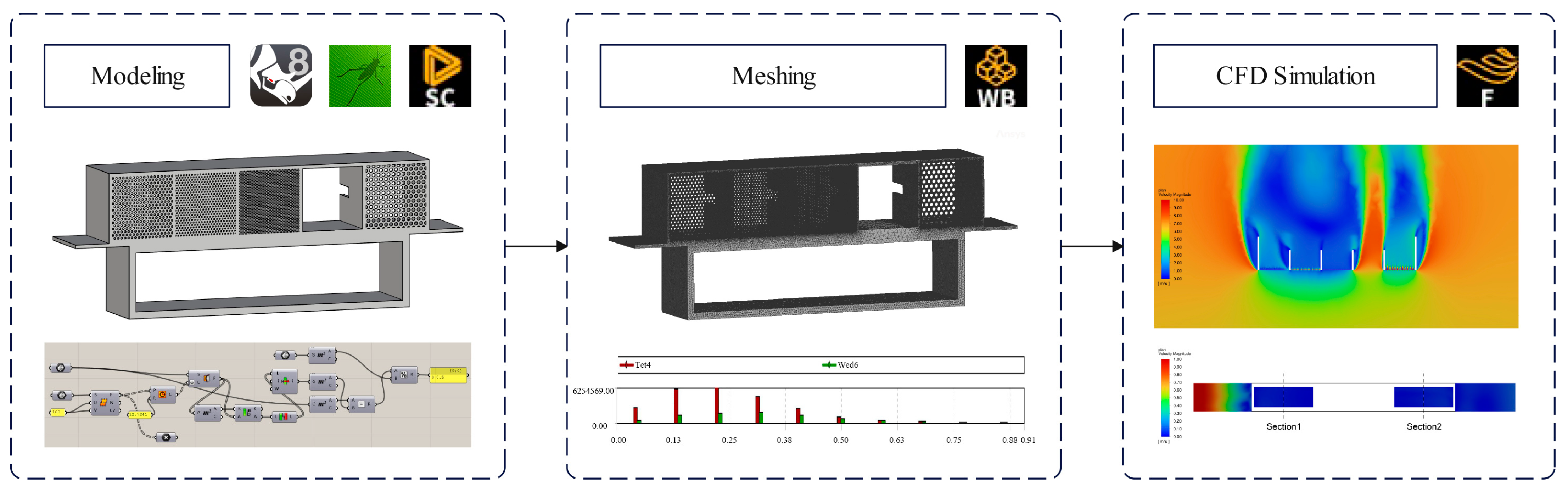
A CFD model was created using Rhino 8 and Grasshopper, where Grasshopper was primarily employed for modeling the perforated panels. In Section 3.3, given the known hole diameters used in experiments, perforated panels with approximately targeted porosity rates were modeled by maintaining a constant hole size while adjusting the density of the diamond-shaped grid. In Section 3.5, to achieve exact porosity rates in integer multiples of 10%, the diamond-shaped grid density was kept constant while the hole diameter was adjusted accordingly. The models were then imported into SpaceClaim to set shared topology, followed by mesh generation in ANSYS Meshing. Finally, CFD simulations were conducted in ANSYS Fluent 2022 R1 (Figure 1).

The Realizable k-epsilon model was selected as the viscous model. When fluid passes through a perforated plate, it undergoes acceleration, contraction, and then sudden expansion. This process is accompanied by high strain rates, flow separation, and vortex generation. Compared to the Standard k-ɛ model, the Realizable k-ɛ model introduces strain rate-dependent variables and imposes constraints on the calculation of turbulent viscosity, enabling more physically accurate predictions of turbulent kinetic energy (k) and turbulent dissipation rate (ɛ) for flows with high strain rates and strong adverse pressure gradients. This is crucial for accurately predicting the resistance characteristics of perforated plates and the resulting flow field structure [19,20,29]. The Scalable Wall Functions were chosen as the wall functions. These functions are insensitive to mesh size, highly robust, and provide stable near-wall solutions even under complex pressure gradients, thereby reducing the difficulty of generating boundary layer meshes.

3. Results

3.1. Wind Tunnel Experiment

3.1.1. Experimental Model

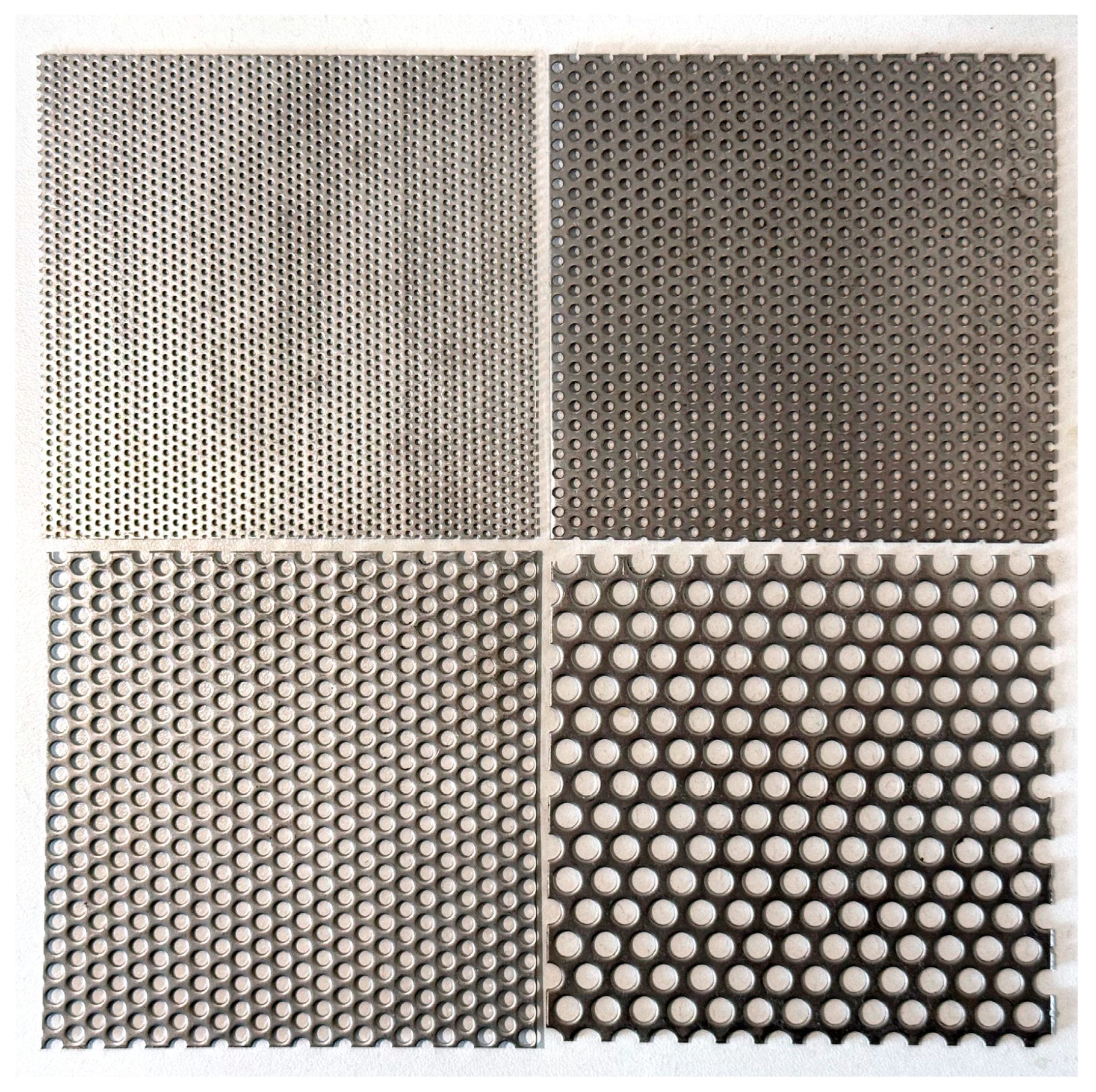
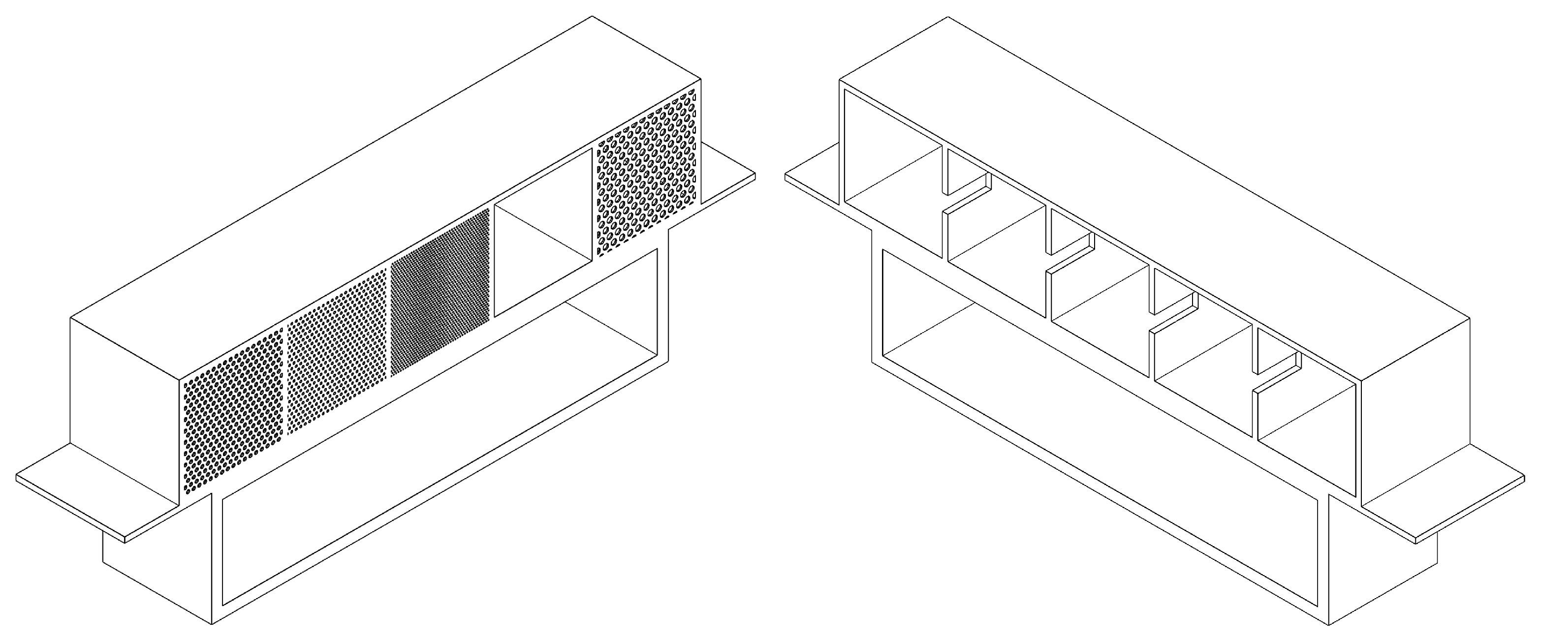
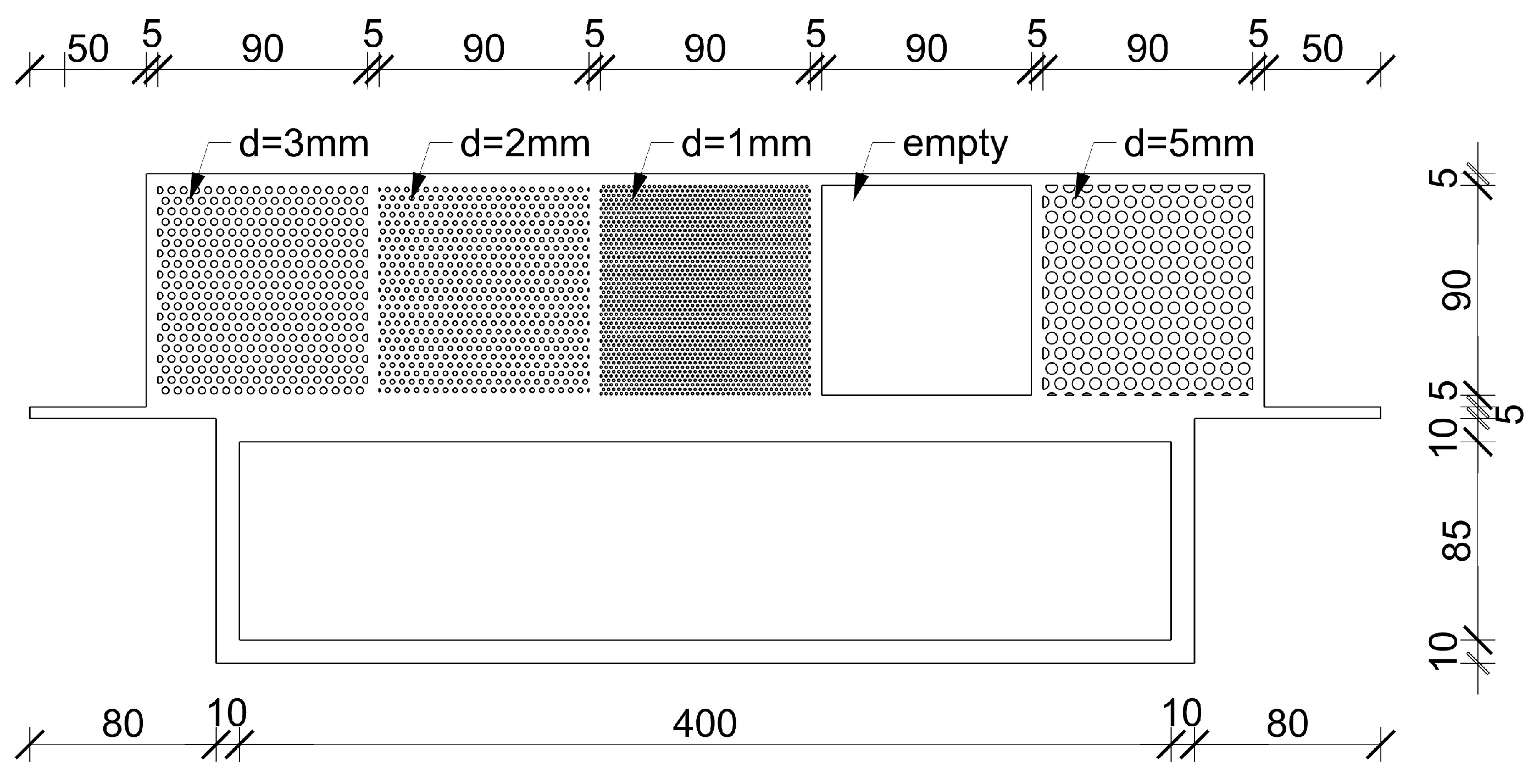
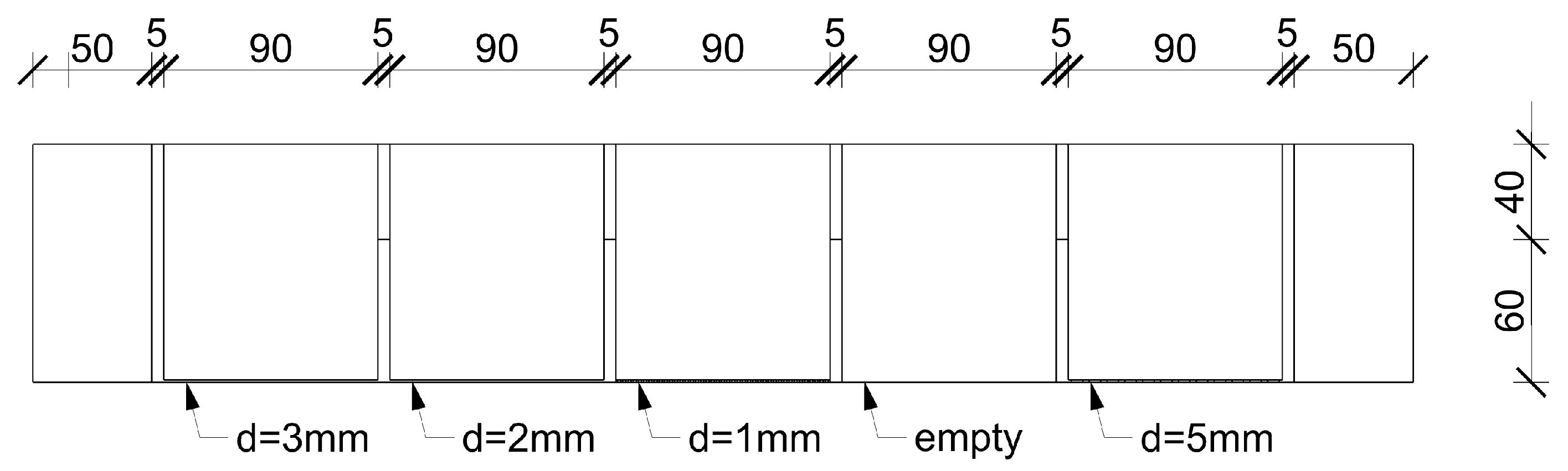
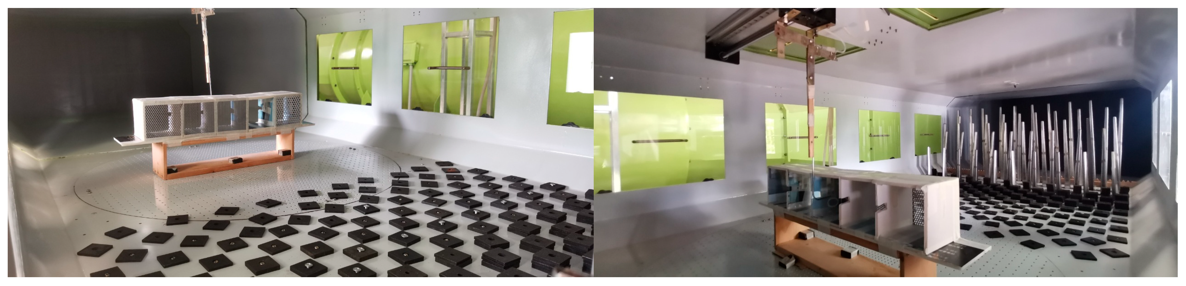
Five connected rectangular boxes were constructed using PVC panels and perforated plates with four different aperture sizes. The internal net dimensions of each rectangular box measured 90 mm × 90 mm at the windward face, with a depth of 100 mm. The windward faces were equipped with four types of perforated plates and one empty box, while the leeward faces were all left open. The four types of metal perforated plates had aperture diameters of 1 mm, 2 mm, 3 mm, and 5 mm, with porosity rates of 18.7%, 21.3%, 29.3%, and 40.3%, respectively. All plates had a uniform thickness of 1 mm and were made of stainless steel. The experimental model was placed on a 110 mm high wooden stand inside the wind tunnel, with the center point of the model at a height of 160 mm. The geometric scale of the building model was 1:1 (Figure 2, Figure 3, Figure 4 and Figure 5).

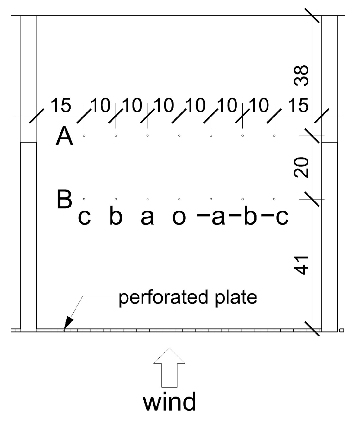
To facilitate the placement of measurement points, four vertical slots (40 mm deep and 15 mm high) were created at the center of the leeward side of each partition plate. Two rows of wind speed measurement points were arranged inside the rectangular box, with 7 points in each row, totaling 14 measurement points (Figure 6).

3.1.2. Wind Tunnel Setup and Experimental Results

The wind tunnel is a boundary layer wind tunnel with a cross-section of 1150 mm × 550 mm and 45 chamfered corners, using a scale of 1:1000 (Figure 7). The mean velocity profile of the incoming flow follows a power-law function with an exponent of 0.25, the wind speed measured at a height of 160 mm above the ground was 6.3 m/s.as shown in Equation (19):

$$v_{\mathrm{Z}}=3.1\times (100\times Z{)}^{0.25}$$

(19)

Table 1. Wind speed measurements at each test point.

Position	5 mm (40.30%)		3 mm (29.30%)		2 mm (21.30%)		1 mm (18.70%)		Empty (100%)
	A	B	A	B	A	B	A	B	A	B
−c	3.61	3.71	−1.20	−1.60	0.95	0.53	1.53	1.78	7.59	7.70
−b	3.39	5.57	2.35	2.23	1.34	1.51	1.57	1.83	7.60	7.74
−a	3.31	3.48	3.56	4.11	1.79	2.16	1.53	1.75	7.64	7.77
o	3.24	3.43	3.51	3.64	2.01	2.22	1.67	1.91	7.69	7.85
a	3.27	3.42	3.29	3.46	1.93	2.08	1.77	2.06	7.72	7.97
b	3.27	3.40	3.26	3.45	1.85	2.26	1.64	2.09	7.48	7.84
c	3.34	3.46	3.39	3.58	1.55	1.40	1.19	0.16	4.83	3.79

presents the measured wind speed values at each monitoring point in the wind tunnel tests for perforated plates with different aperture sizes (1 mm, 2 mm, 3 mm, 5 mm) and an open hole. It can be observed that as the aperture size decreases (with lower porosity), the wind speed significantly declines, indicating that the perforated plates exert a notable obstructive effect on airflow. The open hole (100% porosity) exhibits the highest wind speed, demonstrating unimpeded airflow in the absence of obstructions. The variation in wind speed between different monitoring points (Rows A and B) reflects the non-uniformity of the flow field, which may be attributed to vortex shedding and flow reattachment phenomena behind the perforated plates.

3.2. Full-Scale Model and Simulation

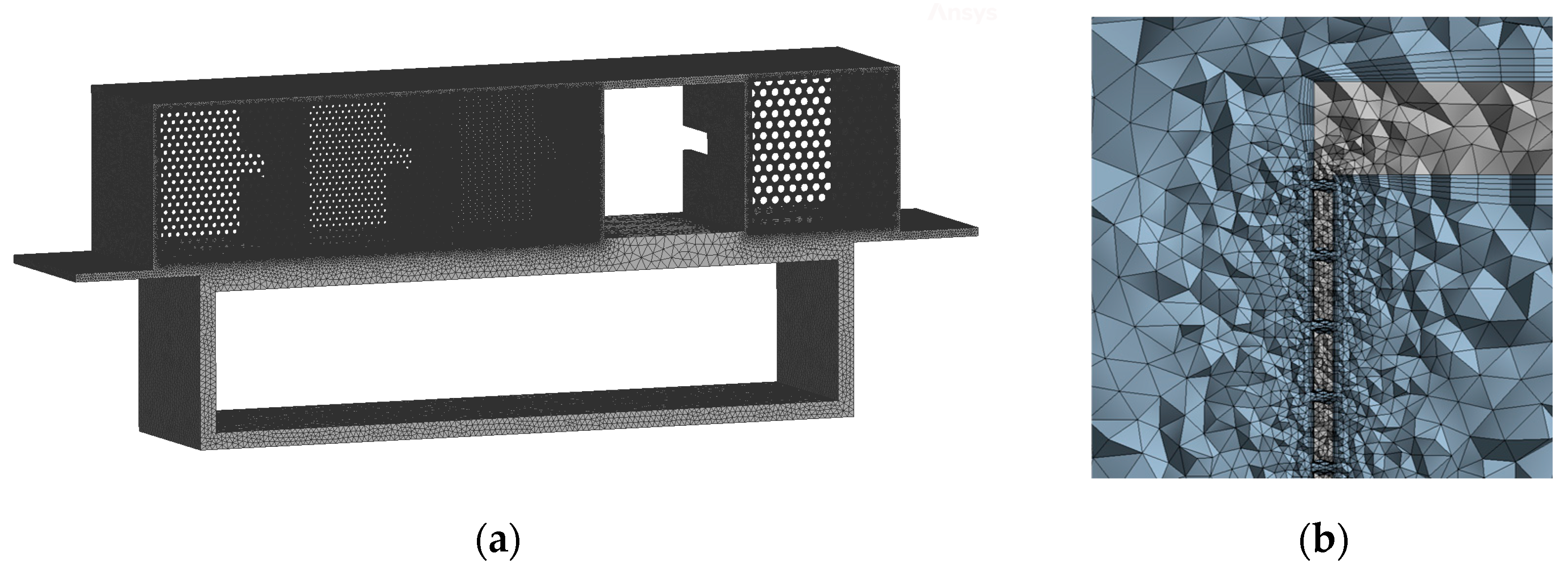
Using the methodology of Section 2.4, a CFD model was constructed that replicates the wind tunnel experimental model (Figure 8). The computational domain dimensions matched the wind tunnel setup.

Table 2. Mesh information of the full-scale model.

Mesh Parameters	Value
Element Size	0.03 m
Inflation Layers	5
Cells	32,086,738
Skewness	<0.90
Average skewness	0.26

presents the mesh information generated for the full-scale model. The maximum skewness is less than 0.9, indicating good mesh quality.

Table 3. Porosity error between models and physical perforated plates.

Aperture Diameter	Physical Sample	Model
1 mm	40.3%	39.94%
2 mm	29.3%	29.83%
3 mm	21.3%	21.14%
5 mm	18.7%	18.99%

presents the porosity errors between the models and physical perforated plates. Due to the modeling approach of fixing the circular hole diameter while adjusting the diamond-shaped grid density, these errors cannot be completely eliminated.

Based on Equation (19), the inlet wind speed profile was set to match the average wind speed profile at the inlet of the wind tunnel test. A user-defined function (UDF) written in C was imported into the computational model in Fluent. The outlet was defined as a pressure outlet, and all other boundary conditions were set as walls.

Table 4. Wind speed at each measurement point using the full-scale modeling method.

Position	5 mm (39.94%)		3 mm (29.83%)		2 mm (21.14%)		1 mm (18.99%)		Empty (100%)
	A	B	A	B	A	B	A	B	A	B
−c	2.91	2.82	0.59	0.55	1.23	1.29	1.36	1.20	7.91	7.70
−b	2.77	2.74	0.61	1.07	1.21	1.26	1.28	1.25	7.91	7.71
−a	2.67	2.70	1.97	2.28	1.20	1.25	1.24	1.24	7.94	7.77
o	2.62	2.70	2.16	2.11	1.24	1.27	1.20	1.23	8.04	7.90
a	2.59	2.67	2.08	2.00	1.28	1.29	1.17	1.22	8.15	8.12
b	2.61	2.74	2.11	2.01	1.34	1.32	1.15	1.19	6.92	8.22
c	2.58	2.71	2.22	2.08	1.46	1.37	1.14	1.20	0.96	1.88

presents the results of the full-scale CFD modeling simulation, which show a consistent trend with the wind tunnel experimental data but exhibit certain numerical deviations. Particularly under small-aperture conditions (e.g., 1 mm), the simulated values are generally lower than the experimental values, which may be attributed to the simplified treatment of local turbulence and orifice effects in the model. Overall, the CFD model effectively captures the fundamental behavior of airflow through perforated plates.

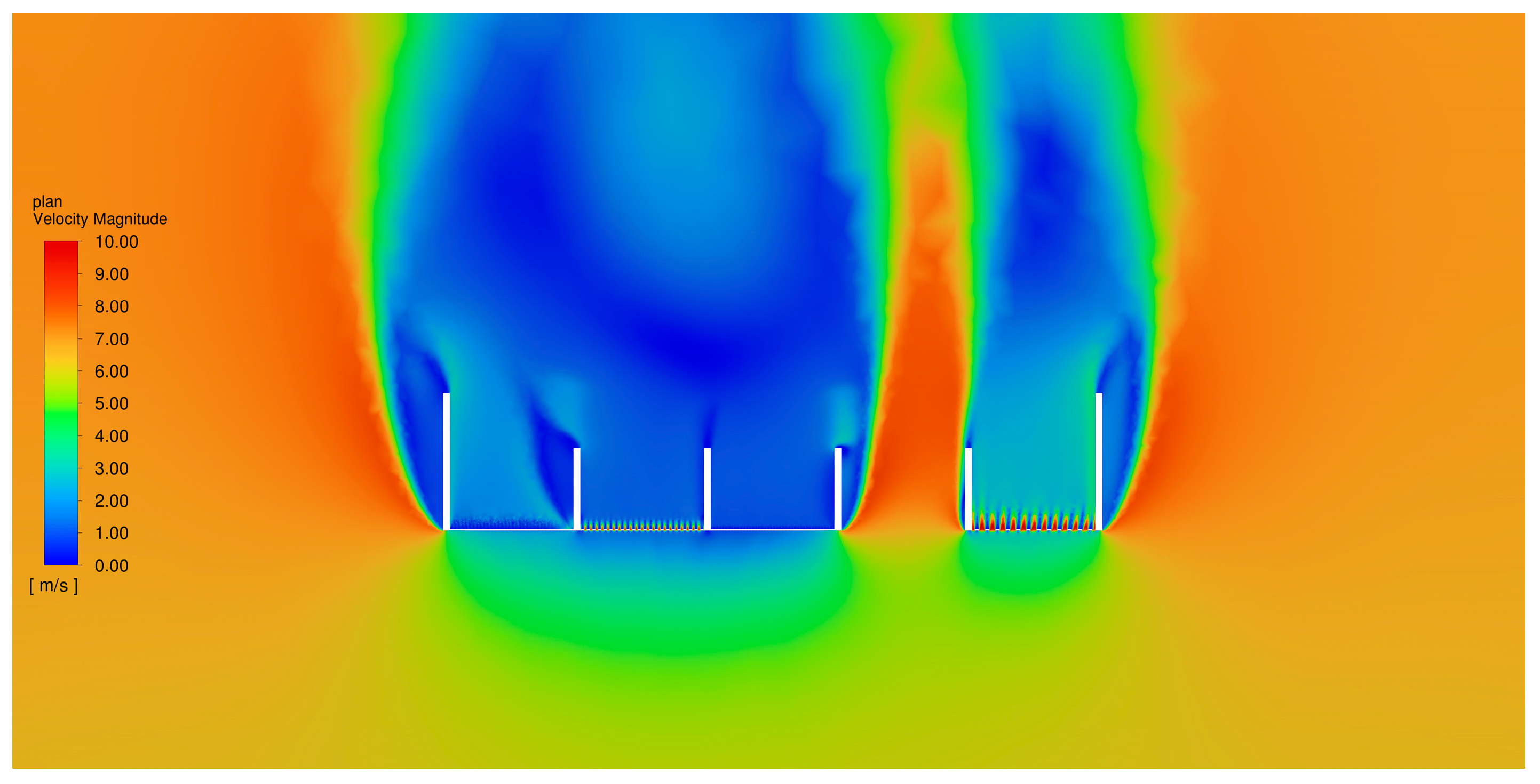
Figure 9 illustrates the velocity distribution of airflow passing through perforated plates with different aperture sizes. It can be observed that the open hole area exhibits the highest wind speed, while a distinct low-velocity zone forms behind the small-aperture perforated plate, indicating its significant obstructive effect on airflow. The contour plot further reveals the redistribution process of airflow behind the perforated plate, aiding in the understanding of local flow field structures.

3.3. Equivalent Simulation of Porous Media

3.3.1. Resistance Parameters of the Porous Medium Model

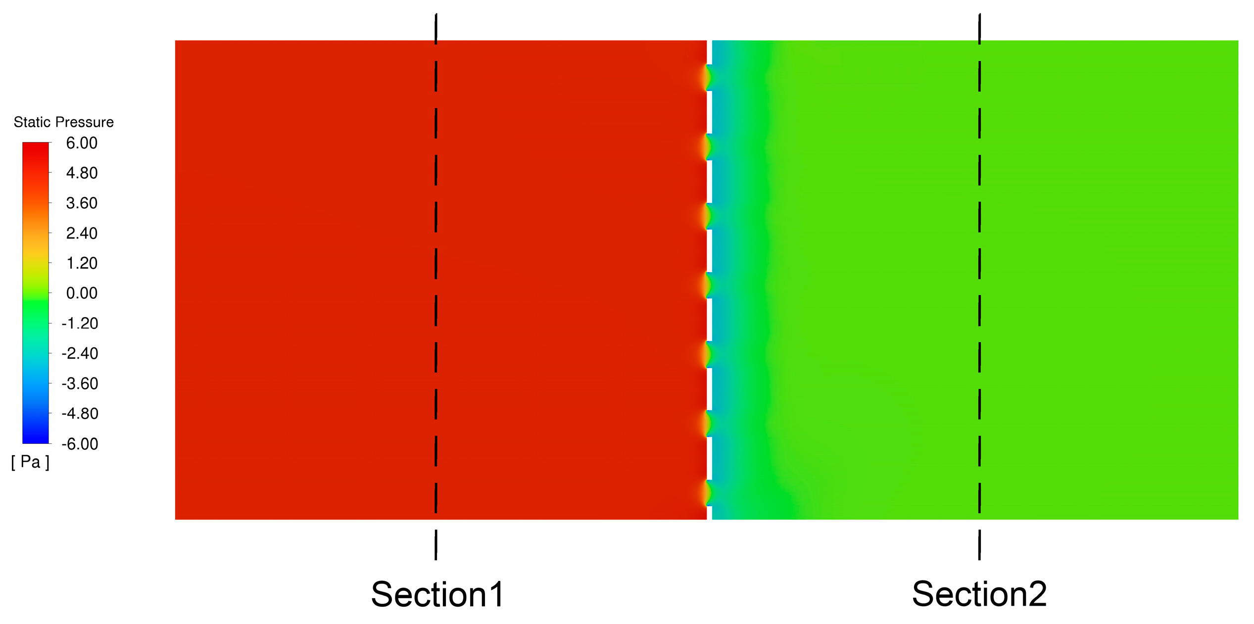
Numerical models of perforated plates with aperture diameters of 1 mm, 2 mm, 3 mm, and 5 mm were established. The perforated plates had dimensions of 90 mm × 90 mm with a thickness of 1 mm, consistent with the experimental specimens. The computational domain length was set to 200 mm (Figure 10). The Realizable k-epsilon model was selected as the viscous model, and Scalable Wall Functions were adopted for near-wall treatment. The inlet velocity was set to 1 m/s, 2 m/s, 5 m/s, 10 m/s, and 20 m/s, respectively, while the outlet was defined as a pressure outlet. The surrounding boundaries of the computational domain were set as symmetric. Pressure monitoring surfaces were placed at 50 mm and 150 mm along the flow direction, where the pressure stabilized, to calculate the pressure gradient under different flow velocities (Figure 11).

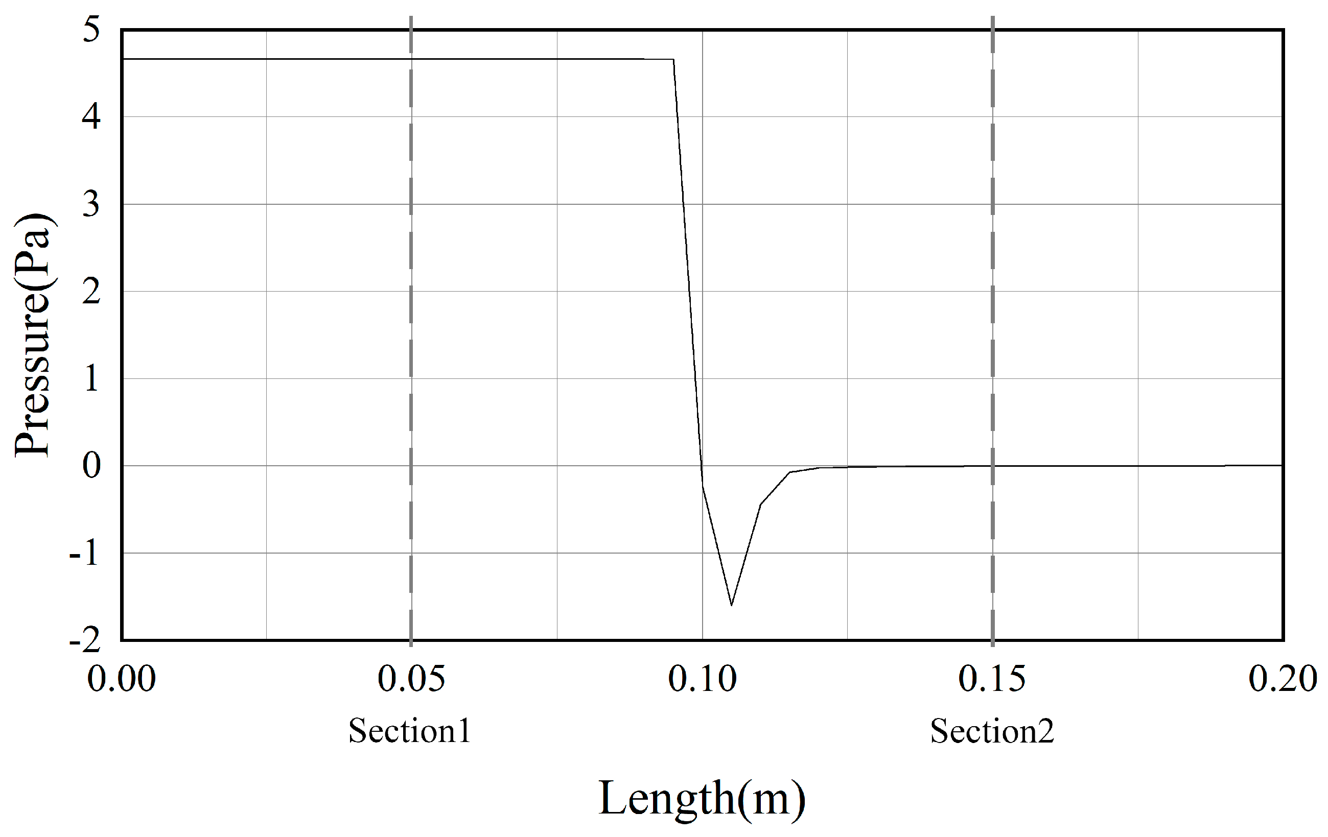
Figure 12 illustrates the pressure distribution along the flow path. A sharp pressure drop is observed immediately after the airflow passes through the perforated panel (at 0.1 m), followed by a gradual stabilization beyond 0.12 m. This trend indicates that the pressure has sufficiently recovered and the flow approaches a fully developed state, validating the rationality of the selected measurement sections (Section 1 and Section 2).

According to Equations (17) and (18) and the pressure drop from

Table 5. Pressure drops corresponding to four types of perforated plates under different wind speeds.

	Velocity (m/s)	Pressure-Before (Pa)	Pressure-After (Pa)	Pressure Gradient (Pa)
d = 1 mm (18.70%)	1	32.37527	−0.002445403	32.3777154
	2	115.1388	−0.01155441	115.1503544
	5	654.9463	−0.0728199	655.0191199
	10	2542.324	−0.2996876	2542.623688
	20	10,221.61	−1.273717	10,222.88372
d = 2 mm (21.30%)	1	23.80617	−0.000284087	23.80645409
	2	89.14614	−0.007091572	89.15323157
	5	547.4971	−0.157672	547.654772
	10	2269.486	−1.526627	2271.012627
	20	9578.111	−11.80715	9589.91815
d = 3 mm (29.30%)	1	10.09048	−0.000499834	10.09097983
	2	37.77029	−0.002585444	37.77287544
	5	227.4448	−0.02313594	227.4679359
	10	919.9766	−0.1272077	920.1038077
	20	3825.252	−0.5977314	3825.849731
d = 5 mm (40.30%)	1	4.665495	−0.003949285	4.669444285
	2	17.75732	−0.02844033	17.78576033
	5	110.7598	−0.3523399	111.1121399
	10	459.0745	−1.426365	460.500865
	20	1903.979	−14.07056	1918.04956

, the Levenberg-Marquardt optimization algorithm was used for curve fitting, with constraints set as a1 ≥ 0, a2 ≥ 0. In the equations, $\Delta n$ = 0.001 m, $\mu =1.7894\times {10}^{-5} \mathrm{P}\mathrm{a}\cdot \mathrm{s},\varrho =1.225 \mathrm{k}\mathrm{g}/{\mathrm{m}}^3$. Based on these values, the viscous resistance coefficient and the inertial resistance coefficient can be calculated (

Table 6. Viscous resistance coefficients and inertial resistance coefficients of the four types of perforated plates.

	a1	a2	1⁄α	C2
d = 1 mm	0.67134	25.5163	37,517,624.914	41,659.2653
d = 2 mm	0	24.34202	0	39,742.0735
d = 3 mm	0	9.66221	0	15,775.0367
d = 5 mm	0	4.85268	0	7922.74286

). In some cases, the optimal fitting result may yield a1 < 0. However, since the pressure drop across thin perforated plates is primarily dominated by inertial losses of the fluid, with minimal viscous losses, it is permissible to set a1 = 0.

3.3.2. Porous Medium Model

A CFD model was created using the method described in Section 2.4, maintaining the same geometry as the wind tunnel test model, but with the perforated plates replaced by solid panels of identical thickness.

Table 7. Mesh information of the porous medium model.

Mesh Parameters	Value
Element Size	0.03 m
Inflation Layers	5
Cells	21,768,062
Skewness	<0.90
Average skewness	0.21

presents the mesh information generated for the porous medium model. Compared to the full-scale model (Table 2), the present model achieves a 32.2% reduction in cell count, indicating a certain degree of improvement in computational efficiency. The maximum skewness is less than 0.9, indicating good mesh quality.

However, due to the minimal panel thickness of 0.001 m, localized mesh density remained high, leading to a substantial number of elements. According to Equation (18), both the viscous resistance coefficient ${\displaystyle \raisebox{1ex}{$1$}\!\left/ \!\raisebox{-1ex}{$\alpha $}\right.}$ and the inertial resistance coefficient C₂ are linearly proportional to the panel thickness $\Delta n$. Therefore, when the plate thickness is increased from 0.001 m to 0.01 m, both ${\displaystyle \raisebox{1ex}{$1$}\!\left/ \!\raisebox{-1ex}{$\alpha $}\right.}$ and C₂ increase by a factor of 10 accordingly, as shown in

Table 8. Viscous and inertial resistance coefficients of the four perforated plate types under different modeled thicknesses.

	$\Delta \mathit{n}$ = 0.001 m		$\Delta \mathit{n}$ = 0.01 m
	1⁄α	C2	1⁄α	C2
d = 1 mm	37,517,624.914	41,659.2653	3,751,762.4914	4165.92653
d = 2 mm	0	39,742.0735	0	3974.20735
d = 3 mm	0	15,775.0367	0	1577.50367
d = 5 mm	0	7922.74286	0	792.274286

.

The plate thickness was increased by a factor of 10, from 0.001 m to 0.01 m, and replaced in the model.

Table 9. Mesh information of porous medium model with increased plate thickness.

Mesh Parameters	Value
Element Size	0.03 m
Inflation Layers	5
Cells	4,619,547
Skewness	<0.90
Average skewness	0.23

presents the mesh information generated for the porous medium model with increased plate thickness. Compared to the full-scale model (Table 2), the present model achieves an 85.6% reduction in cell count, indicating a significant improvement in computational efficiency. The maximum skewness is less than 0.9, indicating good mesh quality.

The corresponding viscous resistance coefficient and inertial resistance coefficient were applied to the two models, respectively, and the solutions yielded are shown in

Table 10. Wind speeds at each measurement point using the porous media equivalence method.

Position	5 mm (39.94%)		3 mm (29.83%)		2 mm (21.14%)		1 mm (18.99%)		Empty (100%)
	A	B	A	B	A	B	A	B	A	B
−c	2.69	2.62	1.46	1.59	1.08	1.13	1.43	1.28	7.93	7.77
−b	2.54	2.51	1.60	1.68	1.10	1.14	1.28	1.23	7.94	7.79
−a	2.45	2.44	1.70	1.75	1.12	1.16	1.19	1.19	7.99	7.85
o	2.37	2.39	1.78	1.78	1.16	1.18	1.14	1.16	8.10	7.98
a	2.29	2.33	1.85	1.81	1.20	1.20	1.09	1.13	8.26	8.23
b	2.22	2.28	1.91	1.84	1.26	1.23	1.05	1.11	7.53	8.20
c	2.20	2.28	1.98	1.89	1.35	1.27	1.01	1.08	1.21	2.61

:

Based on the analysis of data in

Table 11. Wind speeds at each measurement point using the porous media equivalence method with increased plate thickness.

Position	5 mm (39.94%)		3 mm (29.83%)		2 mm (21.14%)		1 mm (18.99%)		Empty (100%)
	A	B	A	B	A	B	A	B	A	B
−c	2.76	2.71	1.37	1.52	1.11	1.15	1.49	1.32	7.92	7.74
−b	2.55	2.57	1.57	1.64	1.11	1.15	1.29	1.27	7.94	7.76
−a	2.47	2.49	1.69	1.73	1.12	1.16	1.21	1.21	8.05	7.84
o	2.38	2.41	1.77	1.78	1.15	1.18	1.15	1.18	8.13	8.02
a	2.32	2.37	1.86	1.83	1.21	1.21	1.09	1.16	8.28	8.25
b	2.27	2.34	1.92	1.87	1.25	1.24	1.06	1.12	6.86	8.49
c	2.28	2.34	2.05	1.97	1.33	1.27	1.04	1.11	0.81	2.19

, significant variations in fluid resistance coefficients are observed across different positions (e.g., −c, −b, −a, o, a, b, c), with noticeable fluctuations as the position changes from the front to the rear of the wind tunnel. As the spacing decreases from 5 mm to 1 mm, the resistance coefficients at all positions increase significantly, indicating that smaller spacings restrict fluid flow and lead to higher resistance. The resistance coefficients at position A are generally higher than those at position B, particularly under small spacing conditions. Furthermore, the perforated plate design in the wind tunnel has a notable impact on fluid flow. The presence of the perforated plate causes local acceleration or deceleration, thereby influencing the overall resistance coefficients.

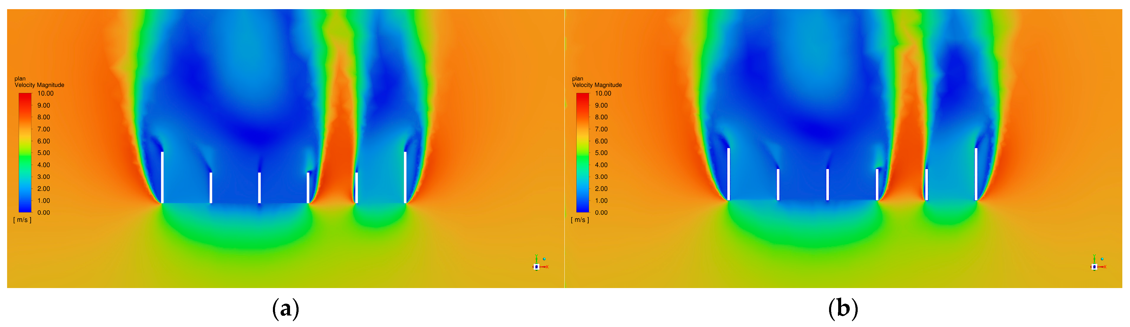
Figure 13 illustrate the wind speed distribution of the porous medium model and the thickened model, respectively. It can be observed that the flow field structures of both models are highly similar, indicating that the thickened model effectively reduces the number of grid elements while maintaining accuracy, thereby improving computational efficiency.

3.4. Data Comparison and Analysis

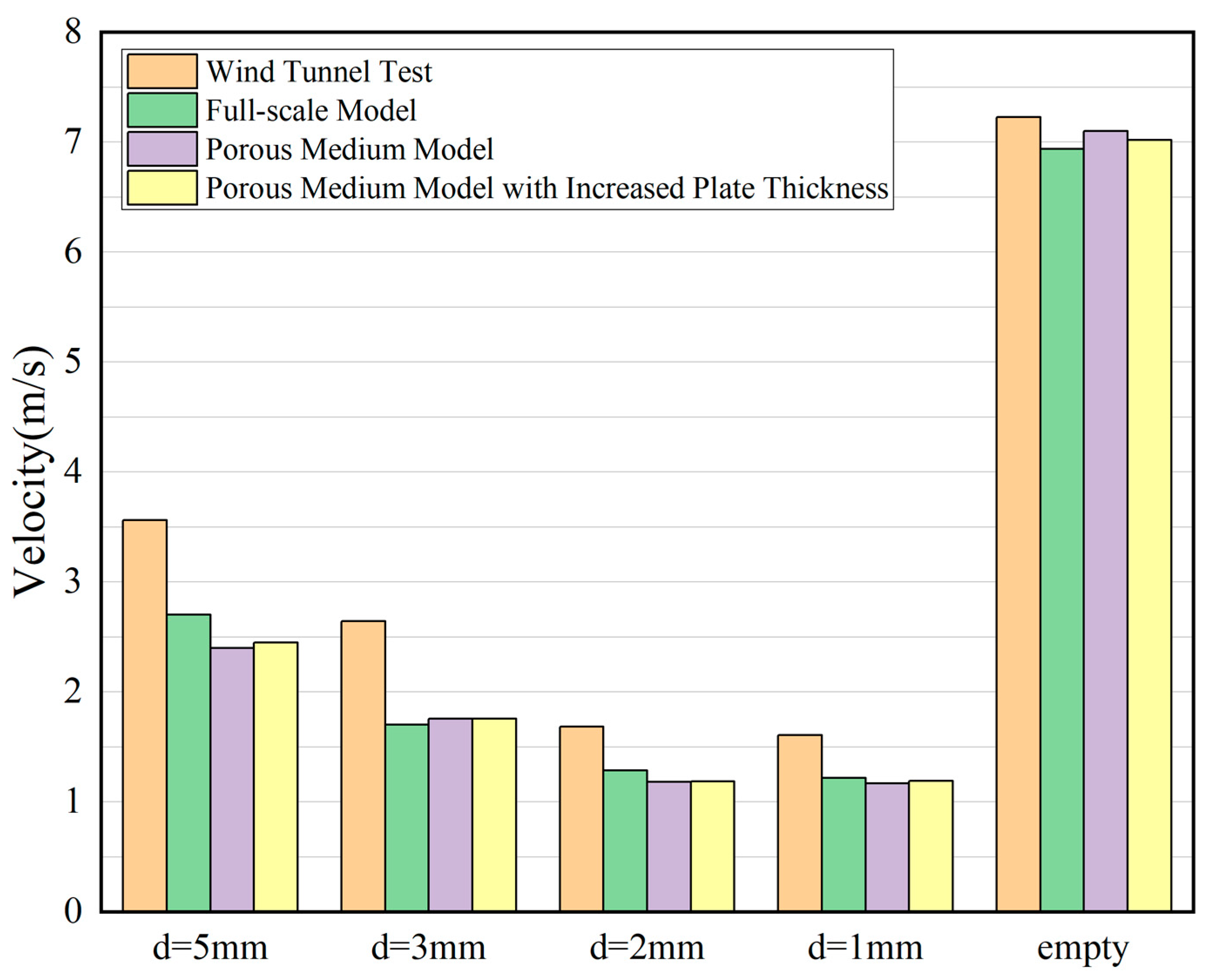
Figure 14 illustrates the variation in wind speed under different aperture conditions (d = 5 mm, 3 mm, 2 mm, 1 mm, and empty) for four models: wind tunnel test, full-scale model, the porous medium model, and the thickened porous medium model. By comparing the wind speeds of different models under various aperture sizes, the influence of aperture dimensions on airflow velocity and the performance differences of each model in simulating airflow through porous structures can be intuitively analyzed. The bar charts in different colors correspond to different simulation or experimental methods, collectively reflecting the consistency and deviations between the predictions of each model and the actual wind tunnel test data. This provides a visual basis for evaluating the reliability and physical rationality of the numerical models. The average of 14 wind speed data points in each box was taken, and one set of experimental data was compared with three sets of simulation data as follows.

From Figure 14, it can be observed that the trends of wind speed variation with aperture size differ significantly under different experimental conditions. Overall, as the aperture diameter decreases (from 5 mm to 1 mm), the wind speed shows a significant declining trend, indicating that smaller apertures impose greater resistance to airflow, leading to a reduction in airflow velocity. The wind speed trends of the four models are generally consistent, though some numerical differences exist. Specifically, at d = 5 mm, the wind tunnel test records the highest wind speed, suggesting minimal airflow resistance through larger apertures in actual measurements. In contrast, the porous medium model and the thickened porous medium model yield relatively lower wind speeds, indicating that the numerical models account for more energy dissipation when simulating airflow through larger apertures, resulting in a slight underestimation of wind speed. As the aperture size gradually decreases to d = 3 mm, d = 2 mm, d = 1 mm, the wind speeds of all models decline significantly. Among them, the full-scale model shows values closer to the wind tunnel test results, demonstrating its stronger capability to replicate real-world conditions under small-aperture scenarios. The porous medium model yields the lowest wind speeds under small-aperture conditions, likely due to its homogenization of fluid flow, which neglects local turbulence effects and further reduces airflow velocity. Notably, under the empty condition, the wind speeds of all models increase significantly and converge closely (around 7 m/s), indicating that in the absence of obstructions, the differences between the models and experimental results are nearly negligible, validating the accuracy and consistency of the model calculations. In summary, the wind tunnel test results are higher under large-aperture conditions but align more closely with simulation results under small-aperture conditions. The porous medium model generally underestimates wind speeds but effectively captures the declining trend as aperture size decreases. The thickened porous medium model demonstrates relatively stable performance across different aperture sizes, suggesting that considering the impact of structural thickness on airflow distribution can enhance the stability and accuracy of the simulation to some extent.

Table 12. Comparative analysis of empty condition data.

	Wind Tunnel Test vs. Full-Scale Model
MAPE (%)	4.02
RMSE (m/s)	0.2908

presents a comparison between wind tunnel tests and full-scale model simulations under empty conditions. By calculating the Mean Absolute Percentage Error (MAPE) and Root Mean Square Error (RMSE), the agreement between numerical simulation results and actual experimental data can be evaluated. Since the cavity contains no obstructions such as perforated plates, the airflow distribution is relatively uniform. Therefore, this comparison is primarily used to validate the reliability and computational accuracy of the baseline model under unobstructed conditions.

From Table 12, it can be observed that the MAPE between the wind tunnel test and the full-scale model simulation is 4.02%, with an RMSE of 0.2908 m/s. These low values indicate minimal error between the two, demonstrating high consistency between the simulation results and experimental data. This suggests that under empty cavity conditions, the model can accurately reproduce the experimental wind speed distribution, with a stable computational process and limited sources of error. It can thus be inferred that the full-scale model exhibits good reliability under unobstructed flow conditions, providing a credible baseline reference for subsequent simulations of complex flow fields involving perforated plates.

Table 13. Comparative analysis of data for four types of perforated plates.

	Wind Tunnel Test vs. Full-Scale Model	Full-Scale Model vs. Porous Medium Model	Porous Medium Model vs. Thickened Porous Medium Model
MAPE (%)	26.89	6.65	1.16
RMSE (m/s)	0.6966	0.1636	0.0263

presents a comparative analysis of wind speed data under four perforated plate conditions. By comparing MAPE and RMSE, the differences between various models can be quantitatively analyzed, and the applicability and accuracy of porous media-type models in simulating complex airflow through perforated plates can be evaluated.

From the results, it can be observed that the MAPE between the wind tunnel test and the full-scale model simulation reaches 26.89%, with an RMSE of 0.6966 m/s, indicating relatively large errors. This suggests a noticeable discrepancy between the experimental and simulation results under perforated plate conditions, which may be attributed to factors such as pore wall friction, local vortices, and turbulent energy dissipation in the actual flow field. In contrast, the MAPE between the full-scale model and the porous medium model decreases to 6.65%, with an RMSE of only 0.1636 m/s, indicating that the porous medium model, while simplifying the computation, still effectively captures the overall characteristics of the airflow. Additionally, the error between the porous medium model and the thickened model is minimal (MAPE = 1.16%, RMSE = 0.0263 m/s), demonstrating nearly identical results between the two. The thickened model further enhances the stability and accuracy of the simulation. The simulation data for the empty condition shows little deviation from the wind tunnel test data, while the simulation data for the perforated plates exhibits moderate but trend-wise similarity to the experimental data. The minimal differences among the three sets of simulation data confirm the rationality and effectiveness of the porous media simulation method.

3.5. Study on Ventilation Performance of Perforated Panel External Windows and Winter Ventilation Strategies

3.5.1. Model Establishment

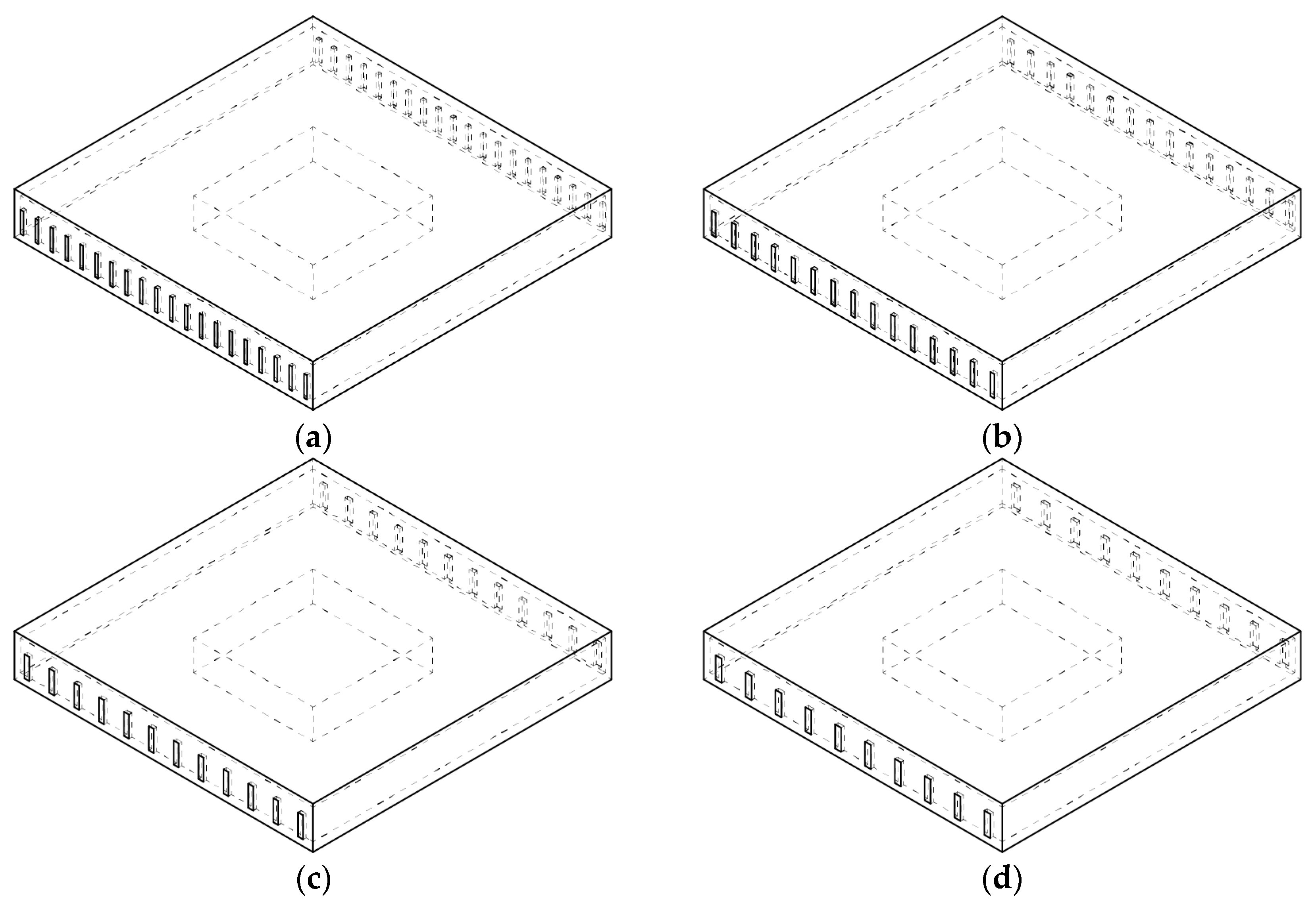
A standard floor model of a high-rise office building was established with a plan dimension of 30 m × 30 m, a floor height of 4.2 m, and an indoor clear height of 3 m. Windows were installed on the windward and leeward facades. The area of a single facade was 126 m², with a fixed window-to-wall ratio of 10% (12.6 m²). The window height was fixed at 2100 mm, while the widths were set to 300 mm, 400 mm, 500 mm, and 600 mm (Figure 15), corresponding to window quantities of 20, 15, 12, and 10, respectively. The wall thickness was 300 mm, and a central core was positioned with plan dimensions of 12 m × 12 m. This setup was used to analyze the impact of different window sizes on ventilation performance under the same window-to-wall ratio. The actual thickness of the metal perforated panels was 3 mm. To reduce mesh count and improve computational efficiency, the model was constructed with a thickness of 300 mm, matching the wall thickness, while the viscous and inertial resistance coefficients were reduced by a factor of 100 accordingly.

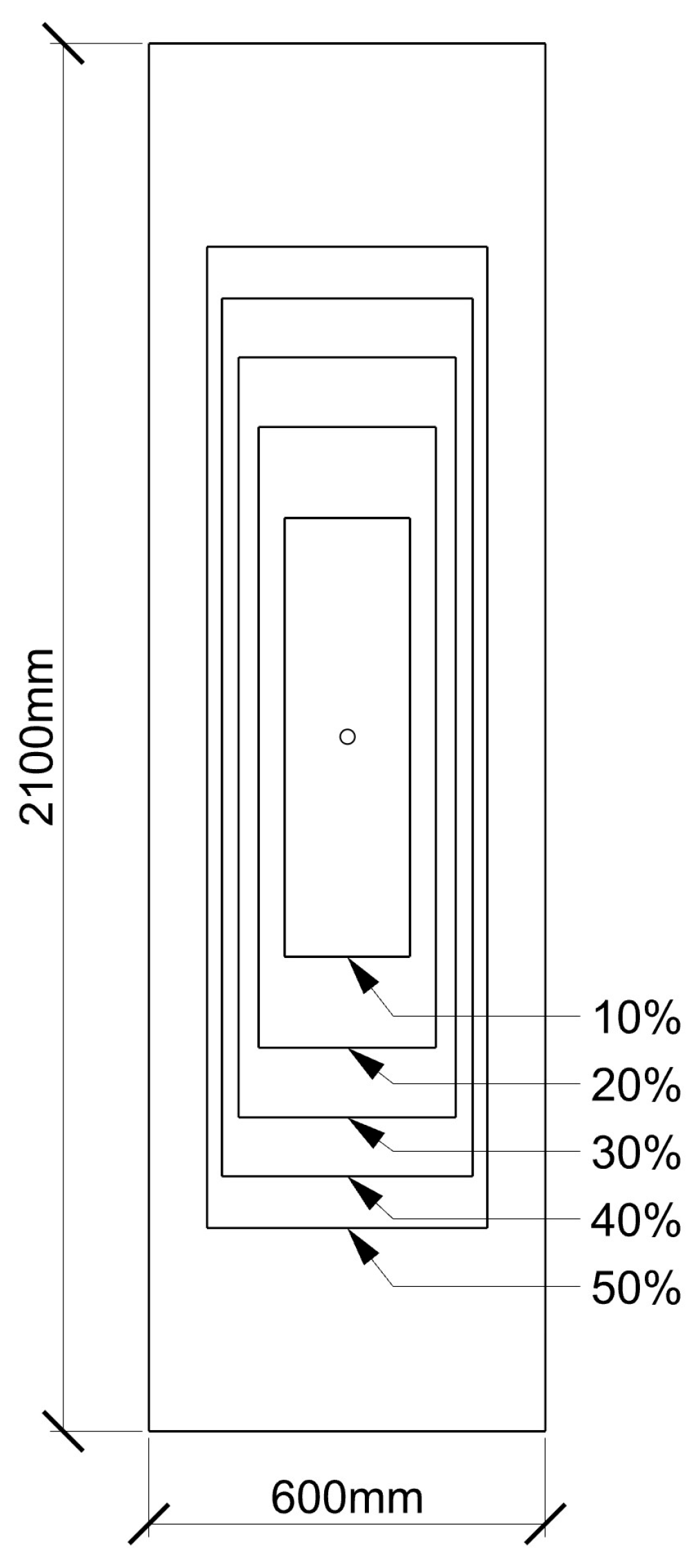
An additional set of open-window models was established as a control group. The effective ventilation area of the control group was consistent with that of the perforated panel models, scaled proportionally based on the center point of the openings. For example, for a window size of 2100 mm × 600 mm with a 50% perforation rate, the corresponding control group opening size was 2100/√2 mm × 600/√2 mm (Figure 16).

3.5.2. Porou Medias Model for Perforated Panels

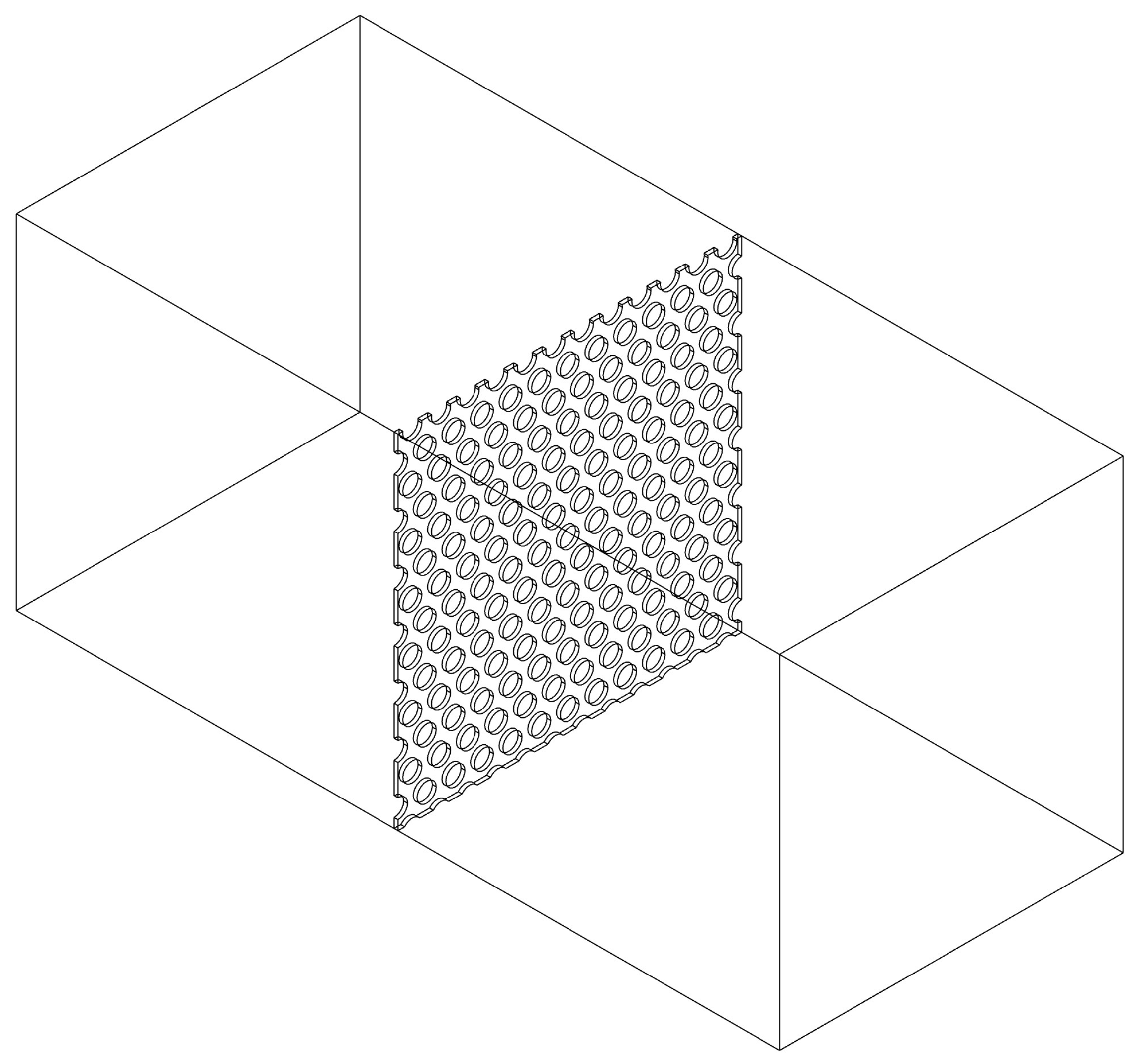
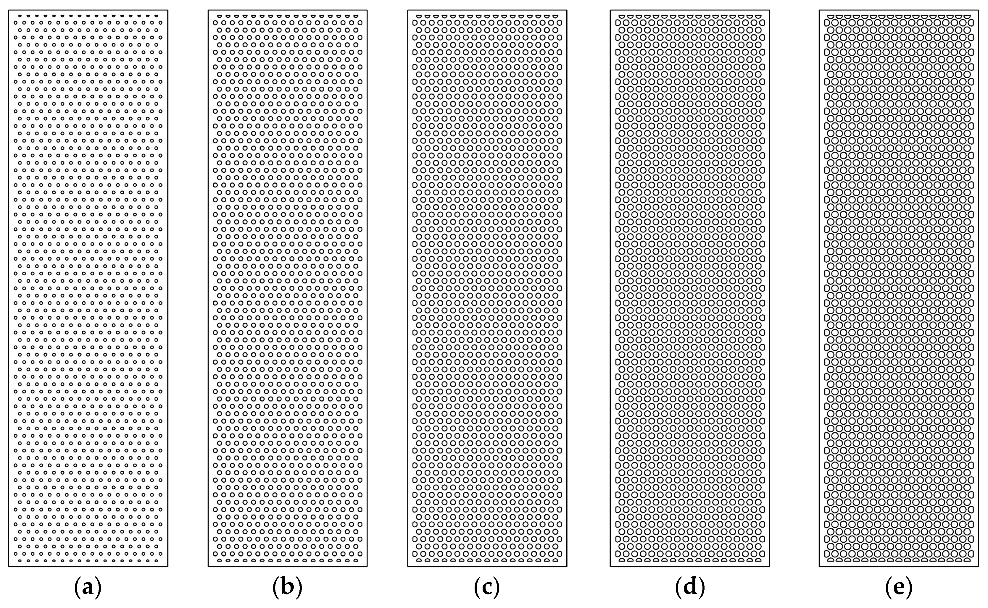
Using Rhino 8 software and the Grasshopper plugin, perforated panels with four widths of 300 mm, 400 mm, 500 mm, and 600 mm were modeled. To ensure the structural integrity of the perforated panels, a 20 mm wide frame was designed around the edges. A perforation rate exceeding 50% would result in excessively close spacing between the circular holes. Therefore, perforation rates were set at five levels: 10%, 20%, 30%, 40%, and 50% (Figure 17).

This study does not address the differences in viscous and inertial resistance coefficients under the same perforation rate but different areas. The method described in Section 3.3.1 was used to obtain the viscous and inertial resistance coefficients for the 20 types of 300 mm thick perforated panels (

Table 14. Viscous and inertial resistance coefficients of the 20 types of perforated panels.

Window Width	Porosity	Viscous Resistance Coefficient	Inertial Resistance Coefficient
300 mm	10%	2,739,873.99	699.77
	20%	659,425.36	152.56
	30%	55,661.73	55.19
	40%	24,779.62	26.65
	50%	16,964.95	14.07
400 mm	10%	516,840.78	664.15
	20%	32,891.67	140.58
	30%	4227.01	54.86
	40%	12,305.09	25.62
	50%	3858.44	13.58
500 mm	10%	1,763,510.40	666.08
	20%	74,118.96	141.10
	30%	182,534.03	59.42
	40%	21,721.47	25.24
	50%	33,302.45	14.38
600 mm	10%	1,236,764.44	663.95
	20%	79,967.22	141.02
	30%	49,126.58	58.58
	40%	28,728.61	26.39
	50%	8323.95	14.03

).

3.5.3. Ventilation Performance Simulation

CFD models for the experimental group (four window widths) and the control group (20 opening configurations) were created using the method described in Section 2.4. The computational domain dimensions were set to 180 m × 150 m × 4.2 m. All 24 models had a uniform element size of 0.5 m with 5 inflation layers, resulting in approximately 10 million grids per model. The maximum skewness was less than 0.90, indicating good mesh quality.

The viscous and inertial resistance coefficients of the perforated panels were imported into Fluent for the experimental group, while no such parameters were applied to the control group. The Realizable k-epsilon model was selected for turbulence modeling, and the Scalable Wall Function (SWF) was used for near-wall treatment. The inlet wind speed was set to 3 m/s, and the outlet was defined as a pressure outlet. All other boundaries were set as symmetric. After reaching steady-state conditions, the average wind speeds $v_1$ and $v_2$ at Section 1 and Section 2 were recorded, and the air changes per hour (ACH) were calculated using the following formula:

$$N=\left(\right(v_1+ v_2)/2\times S\times 3600)/V$$

(20)

where N is the number of air changes per hour (ACH), S is the cross-sectional area of Section 1 and Section 2, V is the volume of indoor air. For all operating conditions in this section, S = 88.2 m², V = 2167.884 m³.

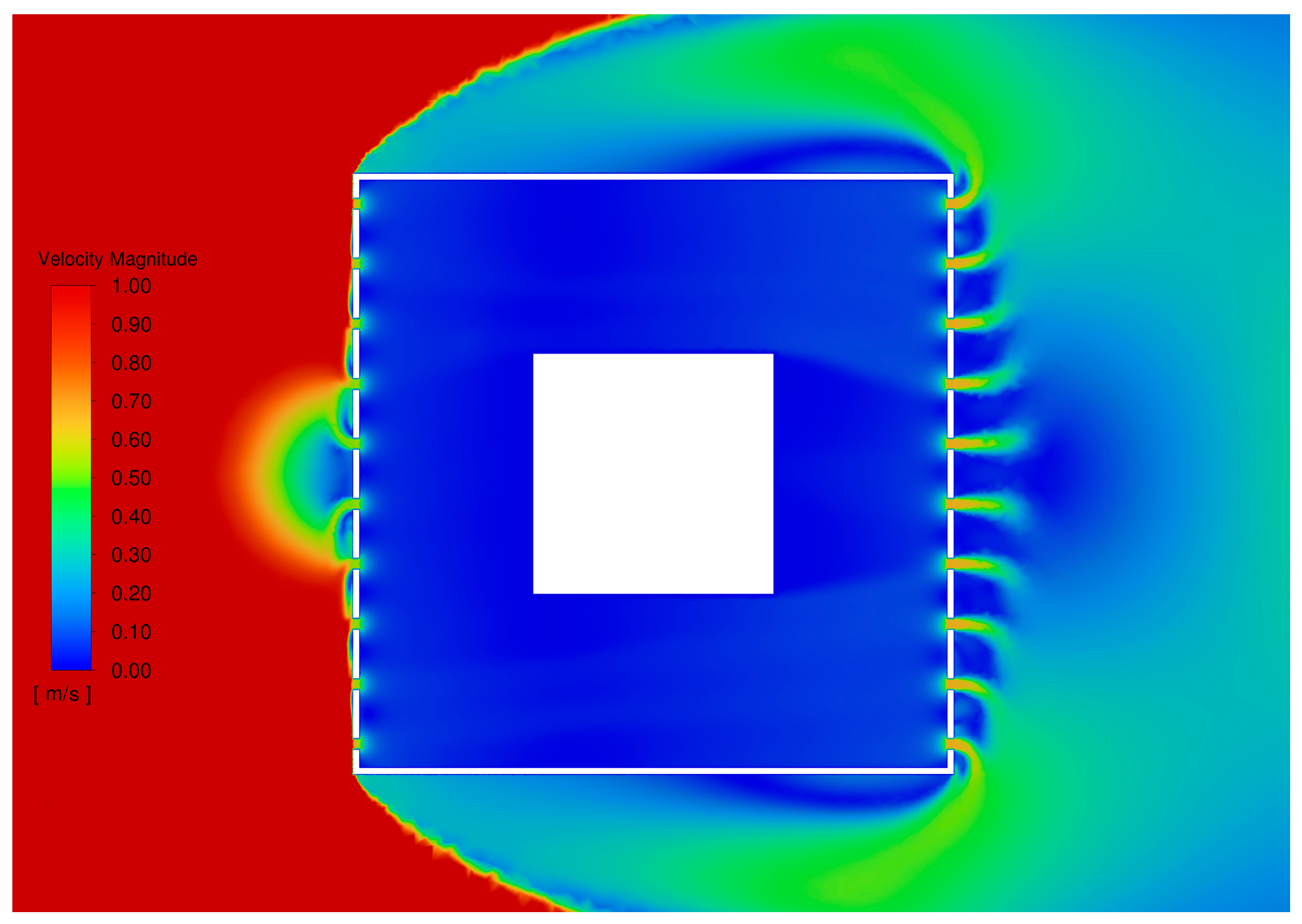
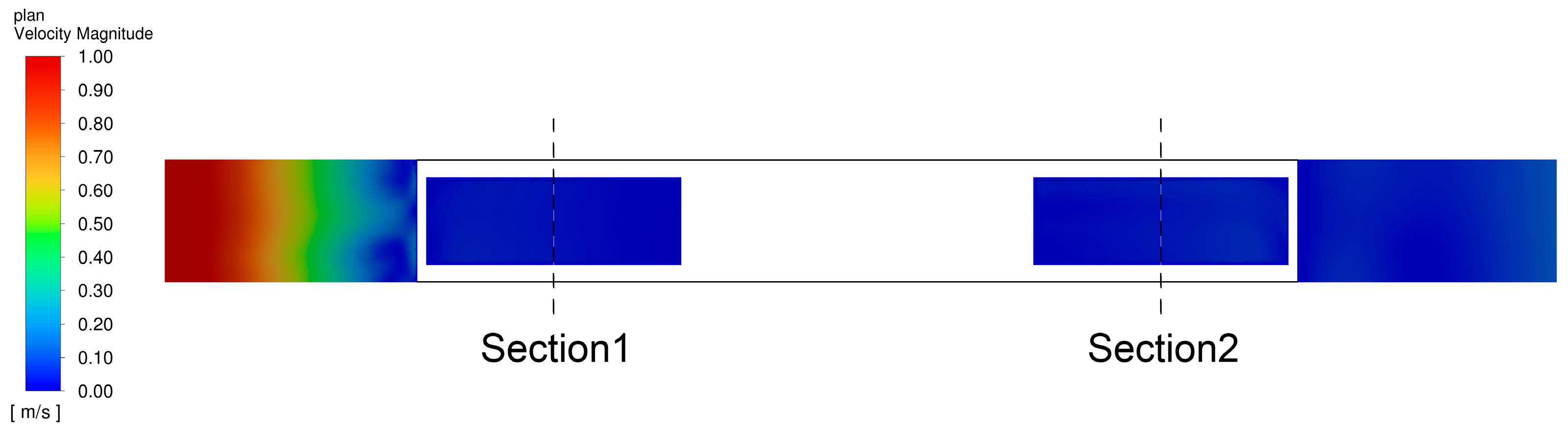
Figure 18 displays the simulated wind speed distribution for a 600 mm wide window with 10% porosity. The upper image illustrates the velocity distribution of the fluid after passing through the porous area. The flow velocity significantly decreases around the pores, forming typical vortex structures. As the airflow enters the porous region, higher-velocity zones concentrate on both sides of the inlet, while low-velocity areas appear around the pores, indicating a clear restriction of fluid flow.

Figure 19 shows the wind speed distribution at two cross-sections (Section 1 and Section 2). The flow velocity is faster at Section 1, while it significantly slows down at Section 2, reflecting the restrictive effect of the pores on fluid flow. Overall, the presence of pores markedly alters the fluid flow path, creating low-speed zones and vortices, which may significantly impact flow resistance and flow field behavior.

Table 15. Air changes per hour for the experimental group.

Porosity	300 mm	400 mm	500 mm	600 mm
10%	6.03	7.32	7.68	7.75
20%	14.23	16.47	20.17	18.16
30%	25.46	26.25	29.37	29.53
40%	35.35	35.94	45.00	41.09
50%	47.11	47.55	55.35	50.09
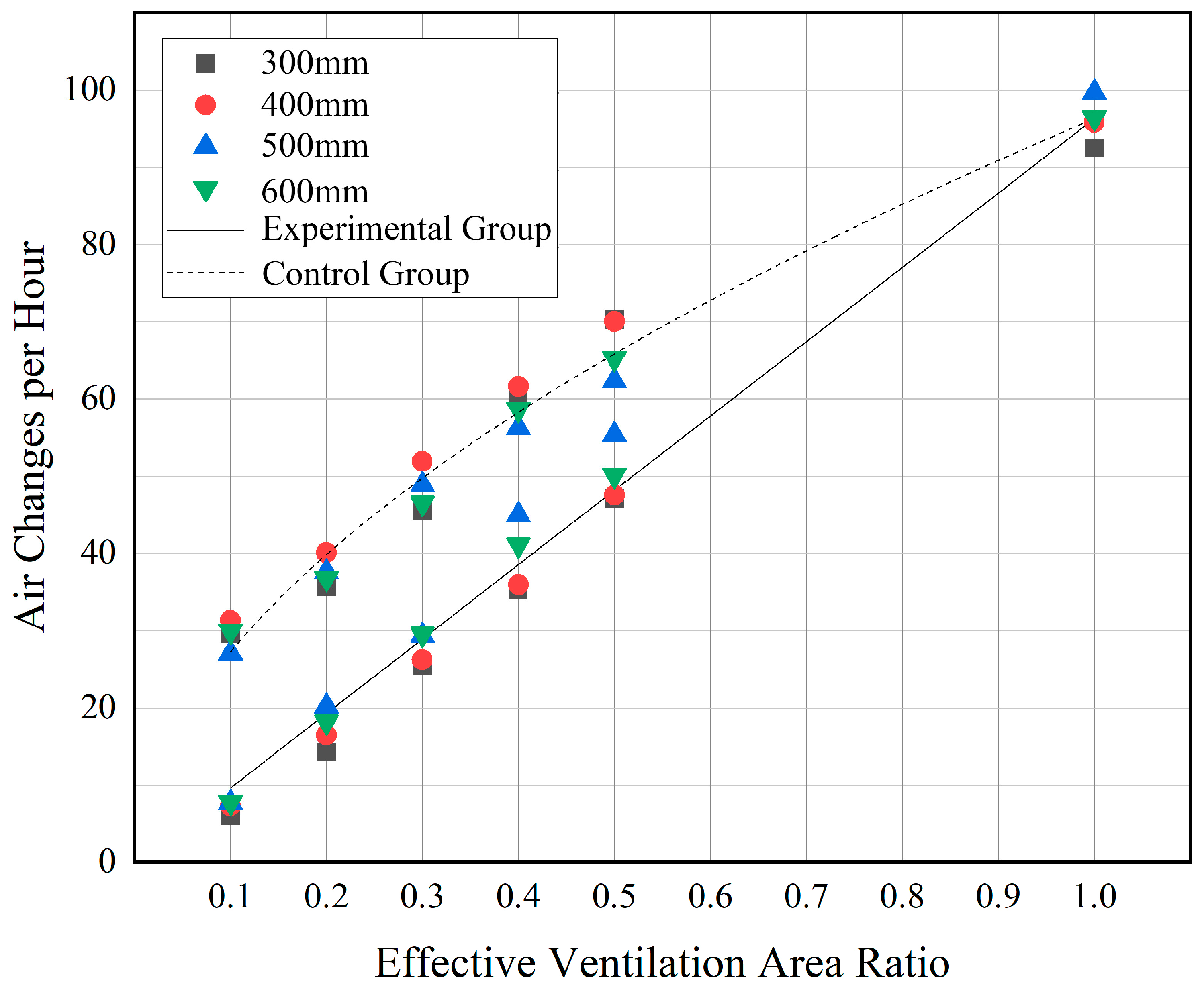
100%	92.49	95.83	99.68	96.44

and

Table 16. Air changes per hour for the control group.

Opening Area	300 mm	400 mm	500 mm	600 mm
10%	29.61	31.33	27.07	29.95
20%	35.69	40.10	37.57	36.75
30%	45.48	51.91	48.90	46.51
40%	60.47	61.62	56.26	58.65
50%	70.26	70.01	62.37	65.25
100%	92.49	95.83	99.68	96.44

presents the air changes per hour (ACH) for the experimental group and the control group under different window widths and perforation rates. It can be observed that the ACH increases significantly with the perforation rate but shows little correlation with the window width. This indicates that the effective ventilation area is the key factor determining ventilation performance, rather than the window size or density. For the experimental group (Table 15), through linear fitting using the equation y = ax, the coefficient a = 96.34 was obtained, with R2 = 0.99587. For the control group (Table 16), using the allometric formula y = axb for fitting, the parameters a = 96.32, b = 0.55, R2 = 0.98259, were obtained. This suggests that the structure of the perforated panels imposes additional resistance to airflow. As shown in Figure 20, although a 50% perforation rate and a 50% opening area share the same effective ventilation area, the ventilation performance of the perforated panels is inferior to that of the open voids.

3.5.4. Winter Ventilation Strategy-A Case Study of Beijing

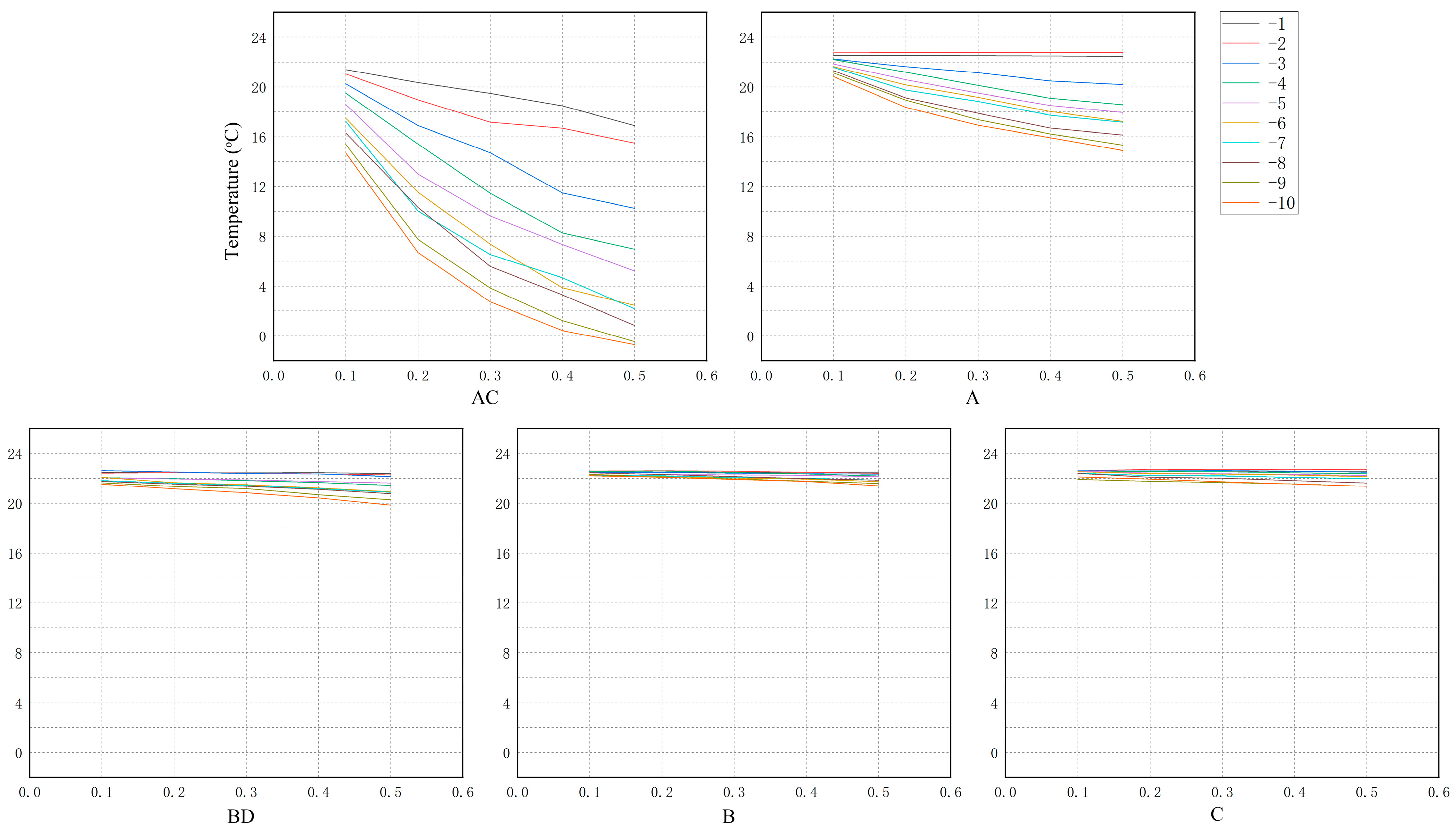
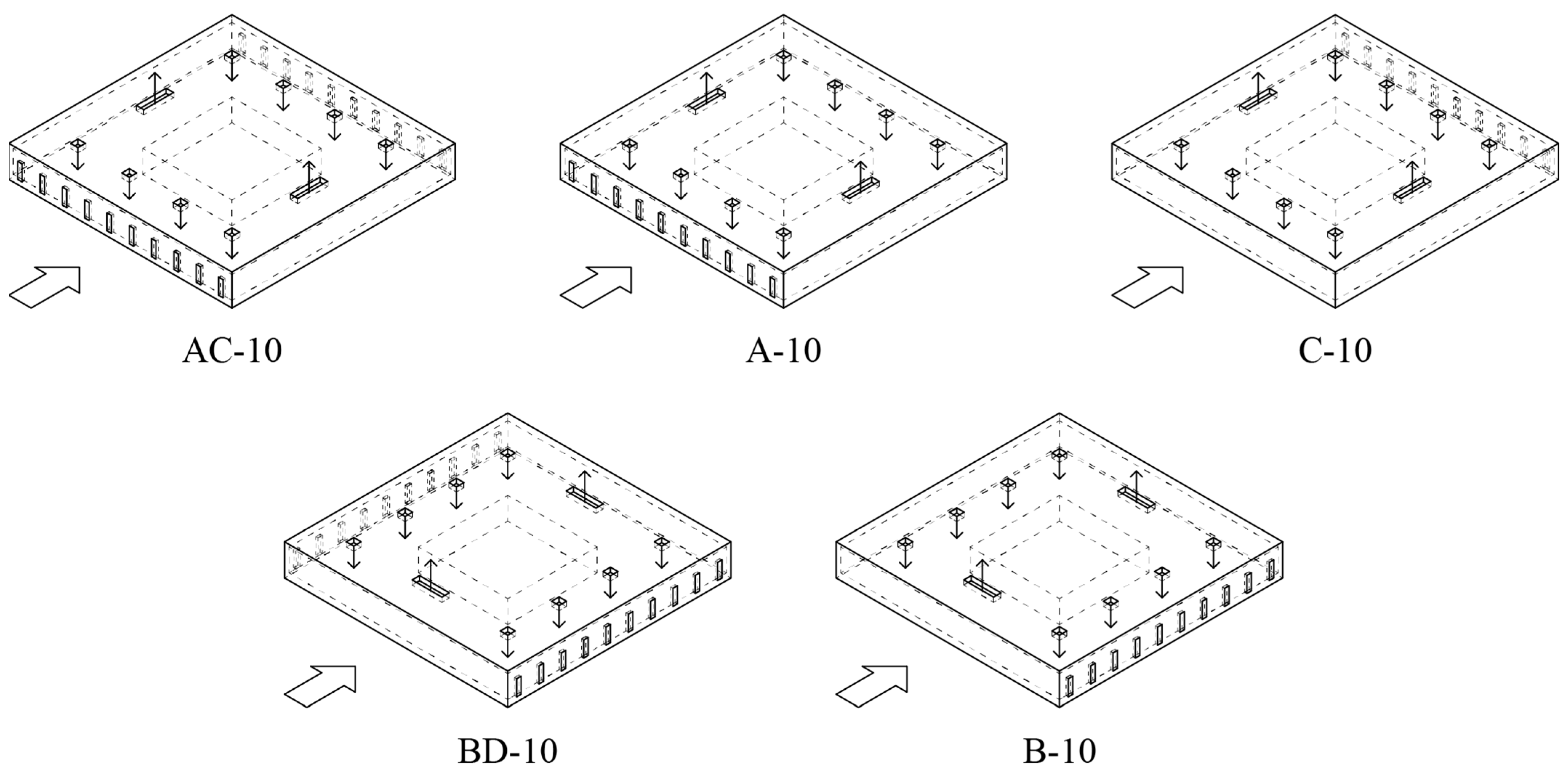
Based on the 600 mm window width model, five operational scenarios were configured: windows open on both windward and leeward facades (AC), windows open only on the windward facade (A), windows open only on the leeward facade (C), windows open on both side facades (BD), and windows open on a single side facade (B). The window area for each scenario accounts for 1% of the facade area, with the number of windows varying from 1 to 10, resulting in 10 operational conditions for each scenario. In each condition, the windows are uniformly distributed on the facade. For example, A-10 (10%) represents a 10% window-to-wall ratio on the windward facade with a 10% perforation rate (Figure 21).

The model assumes winter heating via air conditioning, with 8 supply outlets (each 1 m²) and 2 return inlets (each 4 m²). The supply air temperature is set at 26 °C, and the airflow velocity at both supply and return inlets is 1 m/s. The outdoor wind speed is set to 3 m/s. According to the Chinese standard GB50736 [42], the outdoor design temperature for air conditioning in Beijing during winter is −9.9 °C.

Due to the disturbance caused by the indoor air conditioning supply and return airflow, the outdoor natural ventilation rate cannot be calculated based on cross-sectional wind speed alone. Therefore, the wind speed at the window cross-section is used as the parameter for calculating the air change rate. Choi, Y. and Song, D. verified that even in cases of single-sided ventilation with bidirectional airflow at the opening, the method of measuring inflow air velocity at the opening can accurately calculate the air change rate [43].

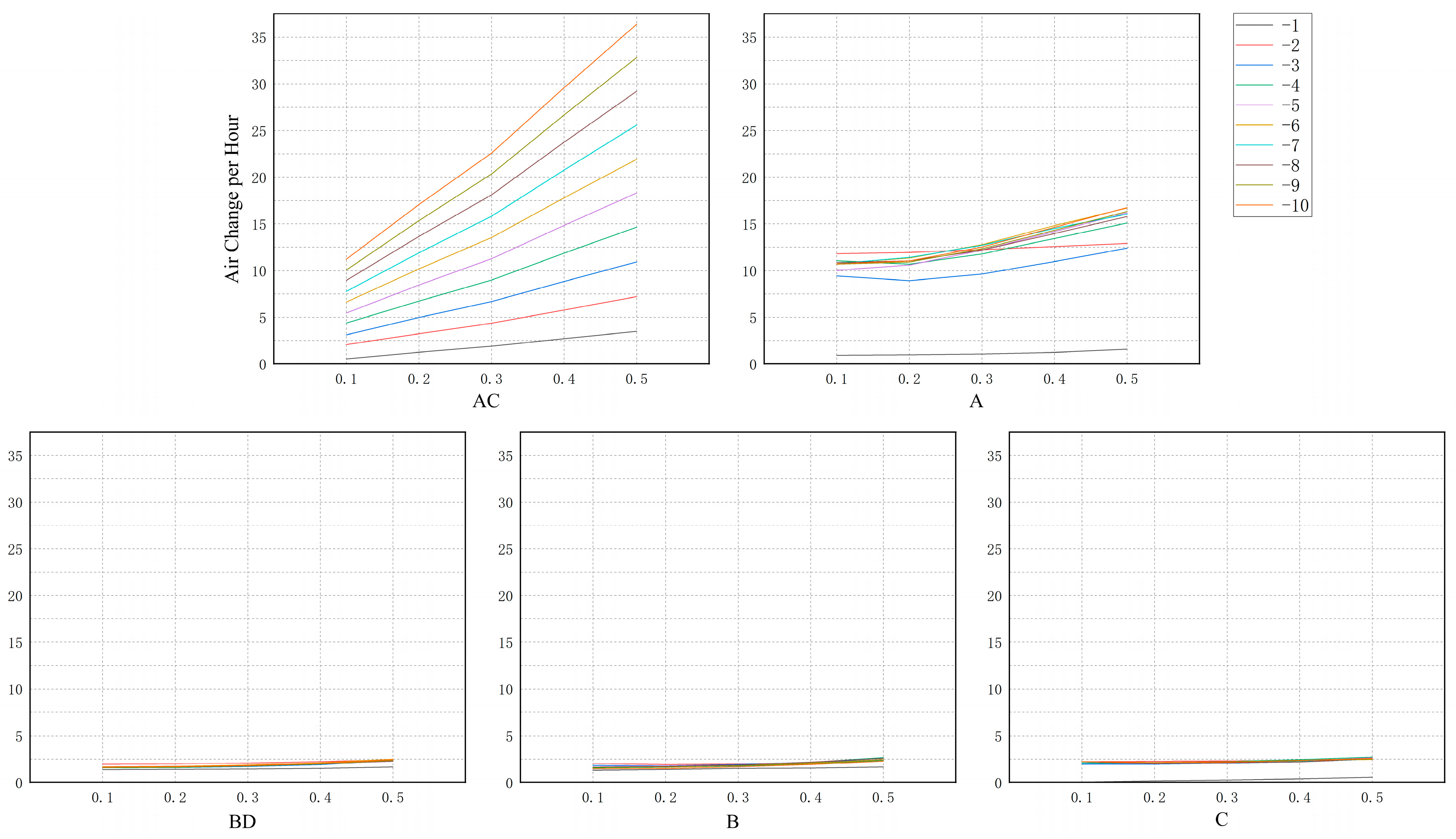
According to the Chinese standard GB50736 [42], the minimum indoor design temperature in winter is 18 °C. Under different window opening configurations and window-to-wall ratios, it is possible to effectively control indoor temperature while ensuring adequate air circulation to achieve a comfortable indoor environment. Different operational conditions of windward façade opening (AC series) and leeward façade opening (A series) significantly impact indoor air change rates and ventilation effectiveness (Figure 22 and Figure 23). For the AC series with windward openings, ventilation performance is relatively poor in cases with smaller opening areas, such as AC-1 (10–40%) to AC-4 (10–10%), where air change rates are generally low. Although these conditions meet the minimum temperature requirements, the insufficient window area limits airflow, preventing effective improvement in air change frequency. In contrast, AC-5 (10%), with an effective ventilation area accounting for 0.5% of the façade area, achieves the highest air change rate of 5.45 ACH, demonstrating better ventilation performance and effectively balancing indoor temperature and air circulation. Therefore, in windward opening designs, moderately increasing the window area is crucial for improving air change rates and ventilation efficiency. In the A series with leeward openings, A-5 (50%) has the largest effective ventilation area ratio of 2.5%, achieving an air change rate exceeding 8.93 ACH, significantly higher than other conditions. This design markedly enhances air exchange frequency, ensuring fresh indoor air, preventing air stagnation, and meeting energy efficiency and comfort requirements. Particularly in the A-2 (10–50%) condition, despite the low porosity, the air change rate remains relatively high, indicating that even with a relatively small window area, reasonable window layout and airflow path design can greatly improve ventilation effectiveness. It is worth noting that the A-1 condition, with only one small window for ventilation, fails to form an effective airflow path, resulting in a low air change rate and poor ventilation performance. Thus, relying on a single airflow path has limitations in improving ventilation efficiency, and such designs should be avoided. Other conditions in the A series, especially A-5 (50%), ensure efficient indoor air circulation by increasing the effective window area and optimizing airflow paths, while simultaneously meeting the minimum winter temperature requirement.

Overall, the window-to-wall ratio is closely related to the air change rate. Reasonably increasing the window area or optimizing airflow paths can significantly enhance ventilation performance. By comprehensively considering different window opening conditions and design parameters, it is possible to ensure the indoor temperature meets the minimum 18 °C requirement in winter while providing adequate air exchange frequency, thereby avoiding indoor air stagnation and excessive temperature issues.

4. Conclusions

This study systematically investigated the ventilation performance of perforated-panel external windows in high-rise office buildings and their applicability in cold regions during winter through wind tunnel experiments and CFD simulations. The main conclusions are as follows:

• This study proposes a method for applying the porous medium model to CFD simulations of perforated panel external window systems, which have already been implemented in practical engineering applications. The porous medium model demonstrates high reliability and applicability in simulating ventilation through perforated panels. Comparative analysis between wind tunnel tests and CFD simulations verifies that the porous medium model accurately captures the resistance effect of perforated panels on airflow. Moreover, it maintains good computational accuracy and efficiency even when the panel thickness is appropriately increased and significantly reduces the number of cells and computation time. This modeling approach supports rapid performance evaluation in early design stages, facilitating the integration of energy-saving strategies into sustainable building workflows.
• Ventilation performance is primarily determined by the effective ventilation area and shows a weak correlation with window size. Under the same window-to-wall ratio, the difference in air change rates across different window widths (300–600 mm) is relatively minimal. The present study does not investigate the underlying causes of this small variation. In contrast, an increase in porosity significantly enhances ventilation capacity. The structure of perforated panels introduces additional resistance to airflow, resulting in slightly lower ventilation efficiency compared to openings of the same area.
• Winter ventilation in cold regions must balance ventilation efficiency and thermal comfort. A case study of Beijing demonstrates that under low outdoor temperatures (−9.9 °C), reasonable control of the window-to-wall ratio (e.g., 0.5–2.5% on the windward side) and porosity (10–50%) can maintain indoor temperatures above 18 °C while achieving air change rates of 5–9 ACH, meeting basic ventilation requirements.
• The window opening configuration significantly influences ventilation performance. Both double-sided openings (e.g., the AC series) and leeward-side openings (e.g., the A series) can achieve satisfactory ventilation effects with appropriate window-to-wall ratios. However, single airflow paths (e.g., only one window) exhibit low ventilation efficiency and should be avoided in design.

References

1. Li, C.; Chen, Y. A multi-factor optimization method based on thermal comfort for building energy performance with natural ventilation. Energy Build. 2023, 285, 112893. [Google Scholar] [CrossRef] [Scilit]
2. Wargocki, P.; Wyon, D.P.; Sundell, J.; Clausen, G.; Fanger, P.O. The Effects of Outdoor Air Supply Rate in an Office on Perceived Air Quality, Sick Building Syndrome (SBS) Symptoms and Productivity. Indoor Air 2000, 10, 222–236. [Google Scholar] [CrossRef] [Scilit]
3. Khdair, A.I.; Aburumman, G.A.; Tahmasbi, F.; Tahmasebi, M.; Kalbasi, R.; Afrand, M. Advancing natural ventilation in sustainable architecture: Mechanisms, innovations, and climate-responsive design for energy-efficient buildings. Renew. Sustain. Energy Rev. 2026, 226, 116314. [Google Scholar] [CrossRef] [Scilit]
4. Santos, H.R.R.; Leal, V.M.S. Energy vs. ventilation rate in buildings: A comprehensive scenario-based assessment in the European context. Energy Build. 2012, 54, 111–121. [Google Scholar] [CrossRef] [Scilit]
5. Southall, R.G. An assessment of the potential of supply-side ventilation demand control to regulate natural ventilation flow patterns and reduce domestic space heating consumption. Energy Build. 2018, 168, 201–214. [Google Scholar] [CrossRef] [Scilit]
6. Huang, K.; Feng, G.; Li, H.; Yu, S. Opening window issue of residential buildings in winter in north China: A case study in Shenyang. Energy Build. 2014, 84, 567–574. [Google Scholar] [CrossRef] [Scilit]
7. EN 13126-5:2011+A1:2014; Building Hardware—Hardware for Windows and Doors—Part 5: Requirements and Test Methods for Hardware for Windows and Doors. European Committee for Standardization (CEN): Brussels, Belgium, 2014.
8. JGJ102-2003; Technical Code for Glass Curtain Wall Engineering. China Building Industry Press: Beijing, China, 2003.
9. Karava, P.; Stathopoulos, T.; Athienitis, A.K. Investigation of the performance of trickle ventilators. Build. Environ. 2003, 38, 981–993. [Google Scholar] [CrossRef] [Scilit]
10. Biler, A.; Unlu Tavil, A.; Su, Y.; Khan, N. A Review of Performance Specifications and Studies of Trickle Vents. Buildings 2018, 8, 152. [Google Scholar] [CrossRef] [Scilit]
11. Jarrahi, A.; Aflaki, A.; Khakpour, M.; Esfandiari, M. Enhancing indoor air quality: Harnessing architectural elements, natural ventilation and passive design strategies for effective pollution reduction—A comprehensive review. Sci. Total Environ. 2024, 954, 176631. [Google Scholar] [CrossRef] [Scilit] [PubMed]
12. GAD + Line + Plus. Viewshine Headquarters. ArchDaily. 2021. Available online: https://www.archdaily.com/979186/viewshine-headquarters-gad-plus-line-plus (accessed on 6 November 2025).
13. Park Associati. Pharo Office Building. ArchDaily. 2021. Available online: https://www.archdaily.com/1004274/pharo-office-building-park-associati (accessed on 6 November 2025).
14. Henning Larsen Architects. SDU Campus Kolding. ArchDaily. 2015. Available online: https://www.archdaily.com/590576/sdu-campus-kolding-henning-larsen-architects (accessed on 6 November 2025).
15. Kasim, N.F.M.; Zaki, S.A.; Ali, M.S.M.; Ikegaya, N.; Razak, A.A. Computational Study on the Influence of Different Opening Position on Wind-induced Natural Ventilation in Urban Building of Cubical Array. Procedia Eng. 2016, 169, 256–263. [Google Scholar] [CrossRef] [Scilit]
16. Zhang, Z.; Yin, W.; Wang, T.; Li, Y.; Zhong, Y.; Zhang, G. Potential of cross-ventilation channels in an ideal typical apartment building predicted by CFD and multi-zone airflow model. J. Build. Eng. 2021, 44, 103408. [Google Scholar] [CrossRef] [Scilit]
17. Yin, S.; van’t Ooster, B.; Ogink, N.W.M.; Koerkamp, P.W.G.G. Assessment of porous media instead of slatted floor for modelling the airflow and ammonia emission in the pit headspace. Comput. Electron. Agric. 2016, 123, 163–175. [Google Scholar] [CrossRef] [Scilit]
18. Liu, Y.; Yang, L.; Hou, L.; Li, S.; Yang, J.; Wang, Q. A porous building approach for modelling flow and heat transfer around and inside an isolated building on night ventilation and thermal mass. Energy 2017, 141, 1914–1927. [Google Scholar] [CrossRef] [Scilit]
19. Hang, J.; Li, Y. Wind Conditions in Idealized Building Clusters: Macroscopic Simulations Using a Porous Turbulence Model. Bound.-Layer Meteorol. 2010, 136, 129–159. [Google Scholar] [CrossRef] [Scilit]
20. Ahn, J.; Kang, J. Enhancing urban CFD simulations with porous media parameters for representative street trees. Ecol. Model. 2026, 512, 111388. [Google Scholar] [CrossRef] [Scilit]
21. Yang, Q.; Rong, L.; Tao, Y.; Tu, J.; Wang, J.; Bai, X.; Hu, Z.; Chai, J.; Wang, Y.; Zhang, G. Similarity analysis and verification of the relationship between resistance coefficients in porous media of different scales: Focusing on slatted floor. Biosyst. Eng. 2025, 257, 104223. [Google Scholar] [CrossRef] [Scilit]
22. Yin, X.; Muhieldeen, M.W.; Razman, R.; Ee, J.Y.C.; Chiong, M.C. The potential effects of window configuration and interior layout on natural ventilation buildings: A comprehensive review. Clean. Eng. Technol. 2024, 23, 100830. [Google Scholar] [CrossRef] [Scilit]
23. Sacht, H.; Lukiantchuki, M.A. Windows Size and the Performance of Natural Ventilation. Procedia Eng. 2017, 196, 972–979. [Google Scholar] [CrossRef] [Scilit]
24. Shetabivash, H. Investigation of opening position and shape on the natural cross ventilation. Energy Build. 2015, 93, 1–15. [Google Scholar] [CrossRef] [Scilit]
25. Allocca, C.; Chen, Q.; Glicksman, L.R. Design analysis of single-sided natural ventilation. Energy Build. 2003, 35, 785–795. [Google Scholar] [CrossRef] [Scilit]
26. Daish, N.C.; Carrilho da Graça, G.; Linden, P.F.; Banks, D. Impact of aperture separation on wind-driven single-sided natural ventilation. Build. Environ. 2016, 108, 122–134. [Google Scholar] [CrossRef] [Scilit]
27. Liu, X.; Wang, H.; Li, Z.; Zhao, J.; Li, C.; Xie, D. Effectiveness of natural ventilation through single-sided window opening in air-conditioning rooms. Energy Build. 2024, 314, 114260. [Google Scholar] [CrossRef] [Scilit]
28. Zhong, H.-Y.; Sun, Y.; Shang, J.; Qian, F.-P.; Zhao, F.-Y.; Kikumoto, H.; Jimenez-Bescos, C.; Liu, X. Single-sided natural ventilation in buildings: A critical literature review. Build. Environ. 2022, 212, 108797. [Google Scholar] [CrossRef] [Scilit]
29. Fallahpour, M.; Ghorbani Naeini, H.; Mirzaei, P.A. Generic geometrical parametric study of wind-driven natural ventilation to improve indoor air quality and air exchange in offices. J. Build. Eng. 2024, 84, 108528. [Google Scholar] [CrossRef] [Scilit]
30. Nasrollahi, N.; Ghobadi, P. Field measurement and numerical investigation of natural cross-ventilation in high-rise buildings; Thermal comfort analysis. Appl. Therm. Eng. 2022, 211, 118500. [Google Scholar] [CrossRef] [Scilit]
31. Miao, S.; Gangolells, M.; Tejedor, B. Validating single-sided natural ventilation models for educational buildings. Build. Environ. 2025, 282, 113329. [Google Scholar] [CrossRef] [Scilit]
32. Tablada, A.; Carmeliet, J.; Baelmans, M.; Saelens, D. Exterior louvers as a passive cooling strategy in a residential building. In Proceedings of the 26th Conference on Passive and Low Energy Architecture, Quebec City, QC, Canada, 22–24 June 2009; pp. 22–24. [Google Scholar]
33. Chandrashekaran, D. Air Flow Through Louvered Openings: Effect of Louver Slats on Air Movement Inside a Space. Master’s Thesis, University of Southern California, Los Angeles, CA, USA, 2010. [Google Scholar]
34. Kosutova, K.; van Hooff, T.; Vanderwel, C.; Blocken, B.; Hensen, J. Cross-ventilation in a generic isolated building equipped with louvers: Wind-tunnel experiments and CFD simulations. Build. Environ. 2019, 154, 263–280. [Google Scholar] [CrossRef] [Scilit]
35. Tai, V.C.; Kai-Seun, J.W.; Mathew, P.R.; Moey, L.K.; Cheng, X.; Baglee, D. Investigation of varying louver angles and positions on cross ventilation in a generic isolated building using CFD simulation. J. Wind Eng. Ind. Aerodyn. 2022, 229, 105172. [Google Scholar] [CrossRef] [Scilit]
36. Teng, X.; Oo, M.L.; Ge, J.; Wong, N.H.; Fan, Y. The improvement of wind comfort and natural ventilation in high-rise building vertical gardens with adjustable louver angles. Build. Environ. 2025, 285, 113638. [Google Scholar] [CrossRef] [Scilit]
37. Kwon, H.J.; Yang, D.S.; Koo, M.S.; Ji, S.M.; Jeong, J.; Oh, S.; Kuk, S.K.; Heo, H.; Ham, D.J.; Kim, M.; et al. Long-lifetime water-washable ceramic catalyst filter for air purification. Nat. Commun. 2023, 14, 520. [Google Scholar] [CrossRef] [Scilit]
38. Zhang, Y.; He, X.; Zhu, Z.; Wang, W.-N.; Chen, S.-C. Simultaneous removal of VOCs and PM2.5 by metal-organic framework coated electret filter media. J. Membr. Sci. 2021, 618, 118629. [Google Scholar] [CrossRef] [Scilit]
39. Song, Y.; Gu, Z.; Liu, S.; Shi, J. Study on applicability of k-ε model for numerical simulation of automobile external flow field. J. Hunan Univ. Technol. 2019, 33, 66–72. (In Chinese) [Google Scholar]
40. Wang, F. Computational Fluid Dynamics Analysis—Principles and Applications of CFD Software; Tsinghua University Press: Beijing, China, 2004; p. 116p. (In Chinese) [Google Scholar]
41. Yan, C.; Qu, F.; Zhao, Y.; Yu, J.; Wu, C.; Zhang, S. Review and challenges of physical models and computational methods in aerospace CFD. Acta Aerodyn. Sin. 2020, 38, 829–857. (In Chinese) [Google Scholar]
42. GB50736-2012; Design Code for Heating, Ventilation and Air Conditioning of Civil Buildings. China Building Industry Press: Beijing, China, 2012.
43. Choi, Y.; Song, D. How to quantify natural ventilation rate of single-sided ventilation with trickle ventilator? Build. Environ. 2020, 181, 107119. [Google Scholar]
Figure 1. Simulation workflow overview.
Sustainability 18 01441 g001
Figure 2. The perforated plates used in the experiment.
Sustainability 18 01441 g002
Figure 3. Axonometric diagram of the test model.
Sustainability 18 01441 g003
Figure 4. Elevation view of the windward side of the test model.
Sustainability 18 01441 g004
Figure 5. Top view of the test model.
Sustainability 18 01441 g005
Figure 6. Top view of the measurement points locations in the test model.
Sustainability 18 01441 g006
Figure 7. Test photograph.
Sustainability 18 01441 g007
Figure 8. Generated mesh: (a) Axonometric diagram and (b) detail of the perforated plate. Both images were captured from ANSYS Meshing.
Sustainability 18 01441 g008
Figure 9. Wind speed contour plots of the full-scale model.
Sustainability 18 01441 g009
Figure 10. Modeling for simulating resistance parameters of perforated plates.
Sustainability 18 01441 g010
Figure 11. Schematic diagram of pressure monitoring surface locations.
Sustainability 18 01441 g011
Figure 12. Pressure distribution along the flow path.
Sustainability 18 01441 g012
Figure 13. Wind speed contour plots: (a) porous media model, (b) porous media model with increased plate thickness.
Sustainability 18 01441 g013
Figure 14. Comparison of wind speed results between the experiment and simulation.
Sustainability 18 01441 g014
Figure 15. Window width models: (a) 300 mm, (b) 400 mm, (c) 500 mm, (d) 600 mm.
Sustainability 18 01441 g015
Figure 16. Correspondence between opening dimensions and perforation rate.
Sustainability 18 01441 g016
Figure 17. Perforated panels with perforation rates of (a) 10%, (b) 20%, (c) 30%, (d) 40%, and (e) 50%.
Sustainability 18 01441 g017
Figure 18. Speed contour plot for a 600 mm window width with 10% porosity.
Sustainability 18 01441 g018
Figure 19. Schematic diagram of wind speed observation surface locations.
Sustainability 18 01441 g019
Figure 20. Curve of air changes per hour vs. effective ventilation area ratio.
Sustainability 18 01441 g020
Figure 21. Five operational conditions.
Sustainability 18 01441 g021
Figure 22. Curve of air change per hour vs. porosity. Plotted based on the data in the Supplementary File.
Sustainability 18 01441 g022
Figure 23. Curve of temperature vs. porosity. Plotted based on the data in the Supplementary File.
Sustainability 18 01441 g023