Heterogeneous Spatiotemporal Graph Attention Network for Karst Spring Discharge Prediction: Advancing Sustainable Groundwater Management Under Climate Change

Abstract

Reliable forecasting of karst spring discharge is critical for sustainable groundwater resource management under the dual pressures of climate change and intensified anthropogenic activities. This study proposes a Heterogeneous Spatiotemporal Graph Attention Network (H-STGAT) to predict spring discharge dynamics at Shentou Spring, Shanxi Province, China. Unlike conventional spatiotemporal networks that treat all relationships uniformly, our model derives its heterogeneity from a graph structure that explicitly categorizes spatial, temporal, and periodic dependencies as unique edge classes. Specifically, a dual-layer attention mechanism is designed to independently extract hydrological features within each relational channel while dynamically assigning importance weights to fuse these multi-source dependencies. This architecture enables the adaptive capture of spatial heterogeneity, temporal dependencies, and multi-year periodic patterns in karst hydrological processes. Results demonstrate that H-STGAT outperforms both traditional statistical and deep learning models in predictive accuracy, achieving an RMSE of 0.22 m³/s and an NSE of 0.77. The model reveals a long-distance recharge pattern dominated by high-altitude regions, a finding validated by independent isotopic evidence, and accurately identifies an approximately 4–6 month lag between precipitation and spring discharge, which is consistent with the characteristic hydrological lag identified through statistical cross-covariance analysis. This research enhances the understanding of complex mechanisms in karst hydrological systems and provides a robust predictive tool for sustainable groundwater management and ecological conservation, while offering a generalizable methodological framework for similar complex karst hydrological systems.

1. Introduction

Distinctive karst landforms originate from the dissolution of soluble carbonate rocks, covering approximately 15.2% of the global land surface. These regions harbor substantial groundwater reserves, serving as a vital freshwater source for nearly 678 million people [1]. Beyond underpinning socio-economic growth, these water assets sustain unique ecosystems and ecological stability [2]. Karst springs serve as natural outlets for pressurized groundwater, with their flow dynamics directly reflecting the aquifer’s recharge and discharge properties. However, the combined strain of climate shifts and escalating human activity has led to persistent water table declines, causing reduced spring discharges and even the risk of complete desiccation [3]. Thus, precise forecasting of spring discharge is paramount for the sustainable management of groundwater resources.

Early research on karst hydrological processes primarily relied on physical mechanisms and numerical modeling techniques. For instance, physically based approaches, such as the double porosity media model, simulate spring discharge dynamics by explicitly characterizing aquifer structures [4]. Similarly, reservoir-based conceptual models employ vertically connected storage units to simulate the nonlinear response of different subsurface zones [5]. However, due to the strong spatial heterogeneity and complex coupled processes in karst systems, these traditional models are limited by parameter uncertainties and structural assumptions, making it difficult to accurately depict the system’s highly nonlinear dynamic behavior [6].

With the rapid development of machine learning techniques, their data-driven nonlinear mapping presents a promising new approach for karst spring discharge prediction. Yousefi et al. [7] applied the Random Forest algorithm to predict groundwater level changes in the karst aquifer of the Hutuo River alluvial fan in the North China Plain, addressing the limitations of traditional statistical models in this region. Nevertheless, standard machine learning methods typically rely on shallow architectures, which limit their ability to capture long-term dependencies and deep structural features within complex hydrological time series.

Deep learning models, through multi-layer nonlinear transformations, have significantly enhanced the modeling capability for nonlinear dynamic processes [8]. Cheng et al. [9] compared the performance of Multi-Layer Perceptrons, Support Vector Regression, and RNNs in predicting karst spring discharge in Northern China, demonstrating that RNNs exhibit superior performance in capturing temporal dependencies. However, standard RNNs suffer from vanishing or exploding gradients when processing long sequences, which limits their ability to learn long-range dependencies [10,11]. To mitigate this, Long Short-Term Memory networks (LSTMs) introduce gating mechanisms to regulate information flow, enabling the learning of dependency patterns over extended periods [11]. Recently, advanced spatiotemporal architectures, including Spatiotemporal Graph Neural Networks (STGNNs), Hierarchical Graph Attention Networks (HGANs), and Transformer-based variants, have been developed to integrate spatial topological learning with temporal sequence modeling [12,13]. While these approaches offer significant improvements, they typically rely on homogeneous graph structures or static connection assumptions, which limit their ability to adequately capture the complex, multi-relational heterogeneity inherent in karst aquifer systems. While these recent models, such as Informer [13] and STGNNs [12], have advanced long-sequence forecasting, they often overlook the semantic differences between spatial neighbors, temporal proximity, and periodic cycles.

The formation of karst spring discharge is intrinsically a multi-source, multi-scale process driven by the interplay of short-term precipitation events, seasonal climate variations, and spatially heterogeneous recharge [14,15,16,17]. A theoretical and methodological challenge remains in effectively capturing these diverse dependencies simultaneously. Most existing frameworks fail to explicitly differentiate the distinct physical mechanisms of spatial connectivity, temporal proximity, and annual periodicity, often treating them as uniform inputs. Consequently, there is a lack of a unified framework capable of adaptively decoupling these heterogeneous relationships and dynamically weighing their contributions to the hydrological response.

To tackle this obstacle, we present a Heterogeneous Spatiotemporal Graph Attention Network, abbreviated as H-STGAT. Utilizing a multi-relational graph framework, this approach effectively delineates the intricate dependencies among spatial, temporal, and cyclical dimensions. The primary contributions of this work are outlined below:

(1)

We propose a novel heterogeneous graph construction strategy that explicitly differentiates between spatial connectivity, temporal proximity, and annual periodicity. This structure overcomes the limitations of homogeneous graphs by preserving the distinct physical meaning of each hydrological dependency.

(2)

We design a hierarchical attention mechanism to independently extract features within each relationship type while dynamically assigning importance weights across different relationships. This enables the model to automatically identify dominant driving factors under varying hydrological conditions.

(3)

We demonstrate that by adaptively decoupling complex spatiotemporal correlations, the proposed H-STGAT significantly improves prediction accuracy for Shentou Spring, offering a robust solution for hydrological time series forecasting in spatially complex karst systems.

The rest of the paper is structured to first present the study area and data materials in Section 2, followed by a detailed explanation of the H-STGAT framework in Section 3. Subsequently, Section 4 and Section 5 display the experimental results and discuss the observations, respectively. Finally, Section 6 summarizes the study’s conclusions.

2. Problem Description

2.1. The Study Area

The Shentou Spring, located in Shentou Town, Shuozhou City, China, serves as the focal point of this study, representing a typical complex karst groundwater system in northern Shanxi Province. Figure 1 shows the location of the study area. The total area of the spring catchment is approximately 4756 km², encompassing parts of Shuozhou City, Xinzhou City, and Datong City [18]. As a crucial water source in the Yanbei region of Shanxi, it supplies municipal water for multiple counties and cities, while also supporting industrial and agricultural development in the area. Shentou Spring represents a unique hydrogeological system, with a basin topography that includes undulating mountains, small basins, and gentle river valleys [19]. The average annual precipitation is 487.3 mm [20]. Precipitation recharges groundwater through surface infiltration, undergoes heterogeneous subsurface transport, and ultimately converges to form the spring. From 1958 to 2020, the mean annual discharge of Shentou Spring was 7.82 m³/s [16,20]. In recent years, due to unsustainable groundwater extraction, the groundwater level has declined, resulting in a continuous decrease in spring discharge, which jeopardizes regional water security and ecological balance [18,19,20].

Precipitation constitutes the predominant recharge mechanism for the spring catchment. There are ten precipitation observation stations within the catchment, located in Kelan, Ningwu, Pianguan, Shanyin, Shenchi, Shuozhou, Yingxian, Youyu, Zuoyun, and Pinglu. To quantify the spatial contribution of rainfall, we employed the Thiessen polygon method to partition the catchment into ten distinct spatial influence zones, as listed in

Table 1. The spatial influence area, its percentage contribution, and the distance to Shentou Spring for each hydrological observation station.

Watershed	Area (km2)	Proportion (%)	Distance (km)
Kelan	165.5565	3.6	64.51737
Ningwu	493.6854	10.7	44.89761
Pianguan	409.3688	8.8	39.05699
Shanyin	391.9116	8.5	15.26839
Shenchi	521.297	11.3	44.75687
Shuozhou	928.1745	20.1	14.1001
Yingxian	332.968	7.2	19.81613
Youyu	476.4325	10.3	38.51526
Zuoyun	376.5716	8.1	39.68096
Pinglu	526.0084	11.4	28.66965
Total	4621.974	100	—

. Unlike physical sub-catchments delineated by topographic divides, these zones define the geometric coverage of each station. The area of these influence zones varies significantly, with a cumulative area of 4621.974 km². The Euclidean distance from each observation station to Shentou Spring exhibits a gradient distribution, ranging from 14.10 km to 64.52 km [16].

2.2. Analysis of Hydrological Data

To gain an in-depth understanding of the intrinsic functioning mechanisms of the Shentou Spring catchment hydrogeological system and to establish a theoretical basis for subsequent predictive modeling, a systematic analysis of the hydrological data from the study area was conducted.

This study compiles monthly scale precipitation data from ten precipitation stations and spring discharge records from the Shentou Spring catchment covering 63 years from January 1958 to December 2020. As shown in Figure 2, all observation stations exhibit distinct seasonal precipitation patterns, with significantly higher rainfall occurring particularly in July and August compared to other months. Figure 2 illustrates the monthly variations in precipitation at ten meteorological stations (a–j), and the observed Shentou Spring discharge (k) plotted as blue lines. Although a similar seasonal rhythm is observed across the stations, notable differences in precipitation intensity and peak timing highlight the spatial heterogeneity of precipitation recharge within the spring catchment.

To systematically investigate the annual cyclical patterns in precipitation data, autocovariance analysis was employed to examine the periodicity of the precipitation time series. The autocovariance $A\left(j\right)$ is calculated as follows:

$$A(j)={\displaystyle \frac{{\sum }_{i=1}^{N-j}(x_i-\overline{x})(x_{i+j}-\overline{x})}{{\sum }_{i=1}^N(x_i-\overline{x}{)}^2}},$$

(1)

where $x_i$ is the $i$-th precipitation sample, $\overline{x}$ is the mean of the precipitation series, $j$ is the separation time (lag) time in months, and $N$ is the total length of the time series. The specific autocovariance for lags of 12, 24, 36, 48, and 60 months is listed in

Table 2. Autocovariance values ($\mathrm{m}{\mathrm{m}}^2$) of monthly precipitation perturbations at specific separation times ($j=12, 24, 36, 48, 60$) for the ten observation stations.

Station	A (12)	A (24)	A (36)	A (48)	A (60)
Kelan	1350.49	1210.23	1238.93	1121.31	1119.24
Ningwu	1296.72	1319.92	1281.29	1191.68	1191.09
Pianguan	1540.26	1556.75	1545.92	1432.33	1452.72
Pinglu	997.37	947.92	927.32	872.15	923.74
Shanyin	1543.58	1554.84	1589.43	1386.61	1402.07
Shenchi	1297.34	1270.25	1281.80	1146.67	1221.62
Shuozhou	1404.56	1330.66	1365.55	1208.39	1301.07
Yingxian	1031.45	989.57	1003.52	869.75	927.81
Youyu	1330.70	1222.63	1290.63	1109.83	1176.25
Zuoyun	1495.89	1497.35	1522.74	1353.27	1388.06

. Figure 3 illustrates the variation in the autocovariance with increasing lag time for the precipitation series. Significant positive peaks occur at lags of 12 months and their integer multiples. This robust periodic fluctuation confirms a distinct and stable annual cycle in regional precipitation, representing a direct manifestation of the seasonal patterns characteristic of the East Asian monsoon climate. As quantified in Table 2, the autocovariance at a 12-month lag remains consistently high across all stations. These numerical results complement the visual patterns shown in Figure 3, collectively confirming the strong annual cyclicity of the regional precipitation.

Since precipitation constitutes the primary source of spring discharge, inherent relationships between these variables are expected to exist. Therefore, we examine the cross-covariance between spring discharge and precipitation at the ten observation sites as a function of lag time, as shown in Figure 4. To eliminate the influence of long-term non-stationary trends, the spring discharge time series were first detrended, and the resulting residuals were analyzed. The formula is expressed as follows:

$$C_{yx}(j)={\displaystyle \frac{1}{N}}{\sum }_{i=1}^{N-j} (y_{i+j}-\overline{Y})\cdot (x_i-\overline{X}),j\ge 0,$$

(2)

where $x$ represents the precipitation time series, $y$ denotes the spring discharge residuals. $i$ is the index sample in the time series dataset, and $j$ indicates the lag time, with the unit of month. $N$ is the total length of the time series. $\overline{Y}$ is the mean of the observed spring discharge residuals, and $\overline{X}$ is the mean of the precipitation time series $x$. Figure 4 illustrates the cross-covariance between monthly precipitation and spring discharge at ten observation sites. The first maximum cross-covariance occurs at a lag of 5 to 6 months, indicating a time delay for precipitation recharge to be converted into spring discharge. In addition, the curve exhibits a distinct 12-month periodicity, with subsequent peaks at lags of approximately 18, 30, 42, 54 and 66 months, reflecting the annual precipitation cycle. Furthermore, the differences among sites confirm that this response is also influenced by spatial heterogeneity within the catchment.

The comprehensive multi-dimensional data analysis demonstrates that the discharge evolution of Shentou Spring is governed by three key mechanisms: spatial heterogeneity in precipitation input, temporal dependence in discharge response, and annual cyclical patterns. Thus, developing a methodology that integrates spatial relationships, temporal dependencies, and annual periodicities into a unified modeling framework can enhance the prediction accuracy of Shentou Spring discharge.

3. Model Structure

This study proposes a Heterogeneous Spatiotemporal Graph Attention Network, designated as H-STGAT, which leverages graph-based structures to integrate hydrologic spatial relationships among observation sites, process-dependent hydrological connections, and periodic hydrological patterns. The model employs attention mechanisms to independently learn hydrological features under each relational context, and subsequently adaptively learns weighting criteria for feature fusion, thereby simulating dynamic precipitation-driven spring discharge.

3.1. Network Architecture

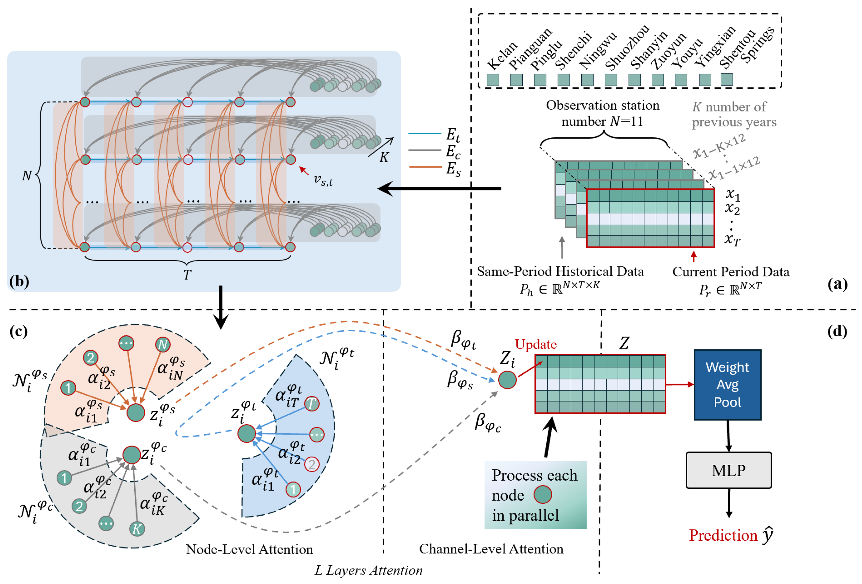
The overall architecture of the model is illustrated in Figure 5. The model input (Figure 5a) comprises recent observations and corresponding historical data from the same periods in previous years. The recent data, denoted as $P_r\in {\mathbb{R}}^{N\times T}$, represents a sequence of precipitation and spring discharge values recorded monthly for the past $T$ months from $N$ observation stations. The historical data from the same period, denoted as $P_h\in {\mathbb{R}}^{N\times T\times K}$, comprises data from the same corresponding months over the past $K$ years. The model updates its input data monthly, ensuring that each prediction is based on the latest continuous observation sequence.

To characterize the spatial hydrological relationships, temporal dependencies, and hydrological periodic patterns, the recent data $P_r$ and the historical data $P_h$ are integrated into a comprehensive graph $G\left(V,E\right)$, where $V$ is the set of nodes and $E$ is the set of edges (Figure 5b).

The node set is defined as $V={\left\{v_{s,t}\right\}}_{s=1 t=1}^{N T+T\times K}$, where $v_{s,t}$ represents an observation value from station $s$ at time step $t$. This set incorporates both the recent observations and the historical same-period observations. Given $N$ stations, $T$ recent time steps, and $K$ years of historical data, the total number of nodes is $N\times T+N\times T\times K$.

The edge set comprises three distinct types of edges designed to capture the heterogeneous dependencies inherent in the hydrological system. The first type is spatial edges, $E_s$, which establish complete connections among nodes from different stations at the same time step. Since subsurface connectivity in karst aquifers is complex and does not strictly decay with Euclidean distance, this fully connected strategy avoids imposing pre-defined geometric assumptions, allowing the model to autonomously learn spatial correlations directly from the data, resulting in a total of $T\times N\times (N-1)/2$ edges. The second type is temporal dependency edges, $E_t$, which sequentially connect nodes from the same station across consecutive months, explicitly modeling the short-term continuity and local trends within the hydrological time series, totaling $N\times \left(T-1\right)$ edges. The third type is cross-year same-month edges, $E_c$, which connect nodes from the recent $T$ months to nodes from the same station and same month in each of the past $K$ years. These explicit connections create shortcuts to historical seasonal patterns, facilitating the capture of long-term periodic dependencies driven by the monsoon climate, amounting to $N\times T\times K$ edges.

To adaptively extract critical information from the spatial hydrological relationships, hydrological process dependencies, and periodic patterns, the model employs a two-layer graph attention mechanism. First, centered on a recent observation node, its neighboring nodes are categorized into three independent computational channels based on the three edge types: the spatial channel ${\phi }_s$, the temporal channel ${\phi }_t$, and the periodic channel ${\phi }_c$. Within each channel, a graph attention mechanism assigns weights to the neighboring nodes and aggregates their information, generating an intermediate representation for the central node specific to that relational perspective, denoted as $Z^{{\phi }_s}, Z^{{\phi }_t},Z^{{\phi }_c}$. Subsequently, the second attention layer evaluates the importance of these three channels and fuses the three intermediate representations via a weighted sum, achieving a comprehensively updated representation for the recent observation node. This process is repeated across multiple layers, enabling each recent observation node to progressively aggregate hydrological information from an expanded neighborhood. Finally, a complete features representation matrix $Z$, encompassing all recent observation nodes, is formed (Figure 5c).

Following this, a weighted average pooling operation is applied to the node representation matrix $Z$ to aggregate the global information from all recent observation nodes, producing a graph-level representation vector $h_G$. Finally, this vector is passed through a non-linear transformation layer to output the predicted spring discharge value for the next time step, ${\widehat{y}}_{t+1}$ (Figure 5d).

3.2. Dual-Level Graph Attention Computation

To adaptively extract features from the multidimensional hydrological relationships embedded in the heterogeneous graph, the core of the model employs a dual-level graph attention mechanism. This mechanism first operates at the node level, learning the importance of neighboring nodes within each independent computational channel. Subsequently, at the channel level, the contributions of the different hydrological relationships to the prediction task are calculated, obtaining a comprehensive feature representation.

In the node-level graph attention computation, we employ the attention mechanism from Graph Attention Networks (GAT) [21] to calculate the importance of neighboring nodes. For a central recent observation node $i$, the model calculates attention coefficients ${\alpha }_{ij}^{\phi }$ between node $i$ and its neighbors ${j\in \mathcal{N}}_i^{\phi }$ within each computational channel $\phi$ (where $\phi \in {\{\phi }_s,{\phi }_t,{\phi }_c\}$) to achieve weighted aggregation. The coefficient ${\alpha }_{ij}^{\phi }$ is computed as follows:

$${\alpha }_{ij}^{\phi }={\displaystyle \frac{exp(\mathrm{ReLU}(a_{\phi }^T[W_{\phi }{h}_i\Vert W_{\phi }{h}_j]))}{{\sum }_{k\in {\mathcal{N}}_i^{\phi }} exp(\mathrm{ReLU}(a_{\phi }^T[W_{\phi }{h}_i\Vert W_{\phi }{h}_k]))}},$$

(3)

where $h_i\in {\mathbb{R}}^d$ is the $d$-dimensional input feature vector of node $i$. $W_{\phi }\in {\mathbb{R}}^{d^{\prime }\times d}$ is a channel-specific linear transformation matrix that projects the node features into a $d^{\prime }$-dimensional space. $a_{\phi }\in {\mathbb{R}}^{2d^{\prime }}$ is the trainable attention parameter vector for channel $\phi$, $\Vert$ denotes the vector concatenation operation, and ReLU is the non-linear activation function. Based on these computed attention coefficients, the model performs a weighted sum of the neighbor nodes’ features, followed by the ReLU activation function $\sigma$, to generate the intermediate representation ${\mathrm{z}}_i^{\phi }\in {\mathbb{R}}^{d^{\mathrm{\prime }}}$ for node $i$ under channel $\phi$. ${\mathrm{z}}_i^{\phi }$ is given as

$$z_i^{\phi }=\sigma \left({\sum }_{j\in {\mathcal{N}}_i^{\phi }} {\alpha }_{ij}^{\phi }{W}_{\phi }{h}_j\right)$$

(4)

After this process is completed for all channels, each central node will possess a set of intermediate representations $\left\{z_i^{{\phi }_s}, z_i^{{\phi }_t},z_i^{{\phi }_c}\right\}$ that encapsulate information from specific hydrological relationships.

Expanding on this, the channel-level attention module is designed to quantify the contribution of various feature channels. The model learns a weight ${\beta }_{\phi }$ for each channel to dynamically adjust the contribution of each hydrological relationship in the final node representation. This weight is calculated using

$${\beta }_{\phi }={\displaystyle \frac{exp(\frac{1}{\left|V_r\right|}{\sum }_{i{\in V}_r}{q}^T ·\mathrm{t}\mathrm{a}\mathrm{n}\mathrm{h} (W_{sem}{z}_i^{\phi }+b_{sem}))}{{\sum }_{k\in \{{\phi }_s, {\phi }_t, {\phi }_c\}} exp(\frac{1}{\left|V_r\right|}{\sum }_{i{\in V}_r}{q}^T ·\mathrm{t}\mathrm{a}\mathrm{n}\mathrm{h} (W_{sem}{z}_i^k+b_{sem}))}},$$

(5)

where ${\mathcal{V}}_r\in {\mathbb{R}}^{\mathrm{T}\times \mathrm{N}}$ is the set of recent observation nodes, while $\mathrm{q},{\mathrm{W}}_{sem},{\mathrm{b}}_{sem}$ are learnable parameters shared across all channels. Finally, the complete representation vector ${\mathrm{Z}}_i\in {\mathbb{R}}^{d^{\mathrm{\prime }}}$ for each recent observation node is obtained by the weighted sum of its intermediate representations across all channels, using the channel weights ${\beta }_{\phi }$. ${\mathrm{Z}}_i$ is given as

$$Z_i={\sum }_{\phi \in \{{\phi }_s, {\phi }_t, {\phi }_c\}}{\beta }_{\phi }·z_i^{\phi }.$$

(6)

This dual-level attention mechanism enables the model to dynamically adjust based on the intrinsic patterns in the data, whether it should rely more on spatial dependencies between stations, temporal dependencies within the observation sequence, or cross-year periodic dependencies for the current prediction step.

3.3. Graph Representation Aggregation and Spring Discharge Prediction

After obtaining the final representation vector ${\mathrm{Z}}_i$ for each recent observation node, it is necessary to aggregate these local features into a global representation vector ${\mathrm{h}}_G$ that captures the current state of the entire hydrological system. A weighted average pooling strategy is adopted. Specifically, the graph-level representation ${\mathrm{h}}_G\in {\mathbb{R}}^{d^{\mathrm{\prime }}}$ is computed by taking a weighted average of the node representation vectors in the matrix $\mathrm{Z}=\left\{{\mathrm{Z}}_i∣i\in {\mathcal{V}}_r\right\}$. ${\mathrm{h}}_G$ is calculated as

$$\begin{gathered} { \mathrm{h}}_{\mathrm{G}}=\sum _{i\in {\mathcal{V}}_r} {\gamma }_i\cdot {\mathrm{Z}}_i, \\ \mathrm{s}.\mathrm{t}.\sum _{i\in {\mathcal{V}}_r}{\gamma }_i=1. \end{gathered}$$

(7)

where ${\gamma }_i$ is a learnable weight assigned to each node $i$.

Finally, to accurately capture the complex nonlinear relationship between the graph-level representation and the prediction target, a Multilayer Perceptron (MLP) is employed to nonlinearly map ${\mathrm{h}}_G$ to the predicted spring discharge at the next time step ${\widehat{y}}_{t+1}$, which is calculated as

$${\widehat{y}}_{t+1}={\mathrm{W}}_{o}ReLU({{\mathrm{W}}_h\mathrm{h}}_G+b_h)+b_o,$$

(8)

where ${\mathrm{W}}_h\in {\mathbb{R}}^{d_h\times d^{\mathrm{\prime }}}$ and $b_h\in {\mathbb{R}}^{d_h}$ are the weight matrix and bias vector of the hidden layer, respectively, and $d_h$ is the hidden layer dimension. ${\mathrm{W}}_o\in {\mathbb{R}}^{1\times d^{\mathrm{\prime }}}$ and $b_o\in \mathbb{R}$ are the weight matrix and bias parameter of the output layer, respectively.

3.4. Evaluation Metrics

To evaluate the predictive accuracy of the model, this study employs four performance metrics to quantify the agreement between observed and predicted data. These are the Root Mean Square Error (RMSE) [22], Mean Absolute Error (MAE) [22], Mean Absolute Percentage Error (MAPE) [23], and the Nash–Sutcliffe Efficiency (NSE) [24]. They are defined as follows:

$$RMSE=\sqrt{{\displaystyle \frac{1}{N}}{\sum }_{i=1}^N{\left(y_i-{\widehat{y}}_i\right)}^2}$$

(9)

$$MAE={\displaystyle \frac{1}{N}}{\sum }_{i=1}^N\left|y_i-{\widehat{y}}_i\right|$$

(10)

$$MAPE={\displaystyle \frac{1}{N}}{\sum }_{i=1}^N\begin{array}{c}\left|{\displaystyle \frac{y_i-{\widehat{y}}_i}{y_i}}\right|\times 100\%\end{array}$$

(11)

$$NSE=1-{\displaystyle \frac{{\sum }_{i=1}^N{\left(y_i-{\widehat{y}}_i\right)}^2}{{\sum }_{i=1}^N{\left(y_i-\overline{y}\right)}^2}}$$

(12)

In the equations above, $y_i$ represents the observed spring discharge value, $\overline{y}$ is the mean of the observed discharges, ${\widehat{y}}_i$ denotes the predicted value, and $N$ is the total number of observations.

The numerical value of NSE falls within the interval $(-\infty ,1]$ and serves to assess the goodness-of-fit between predicted and observed values. An NSE value closer to 1 indicates better model performance. RMSE measures the root mean square deviation between predicted and observed values, indicating their dispersion. MAE represents the mean absolute error. Unlike RMSE, which squares the errors, MAE uses absolute values, thereby assigning equal weight to errors of different magnitudes and making it a more robust metric. MAPE quantifies the mean absolute percentage error between predictions and observations.

4. Experiment

4.1. Experimental Setup

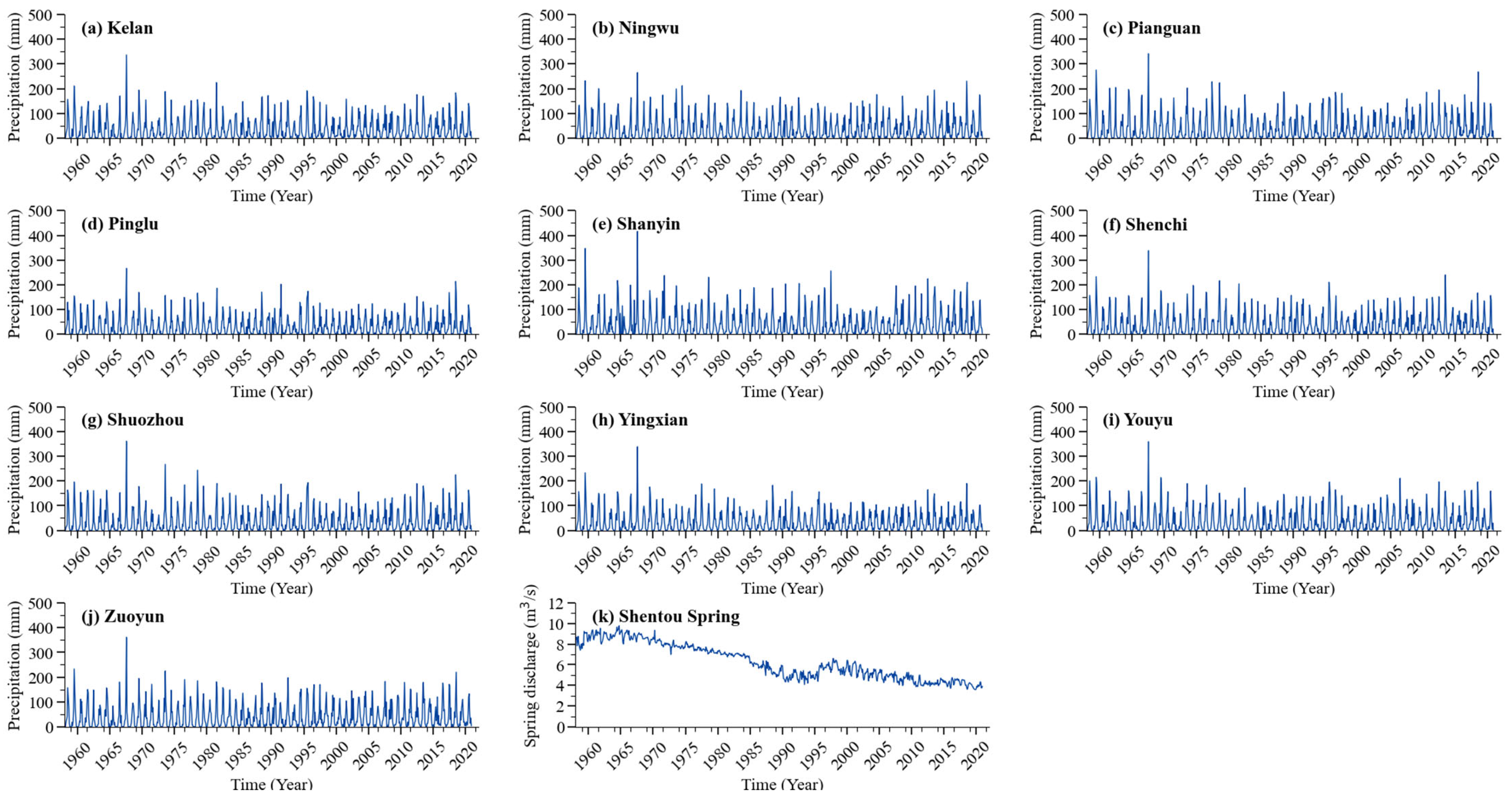
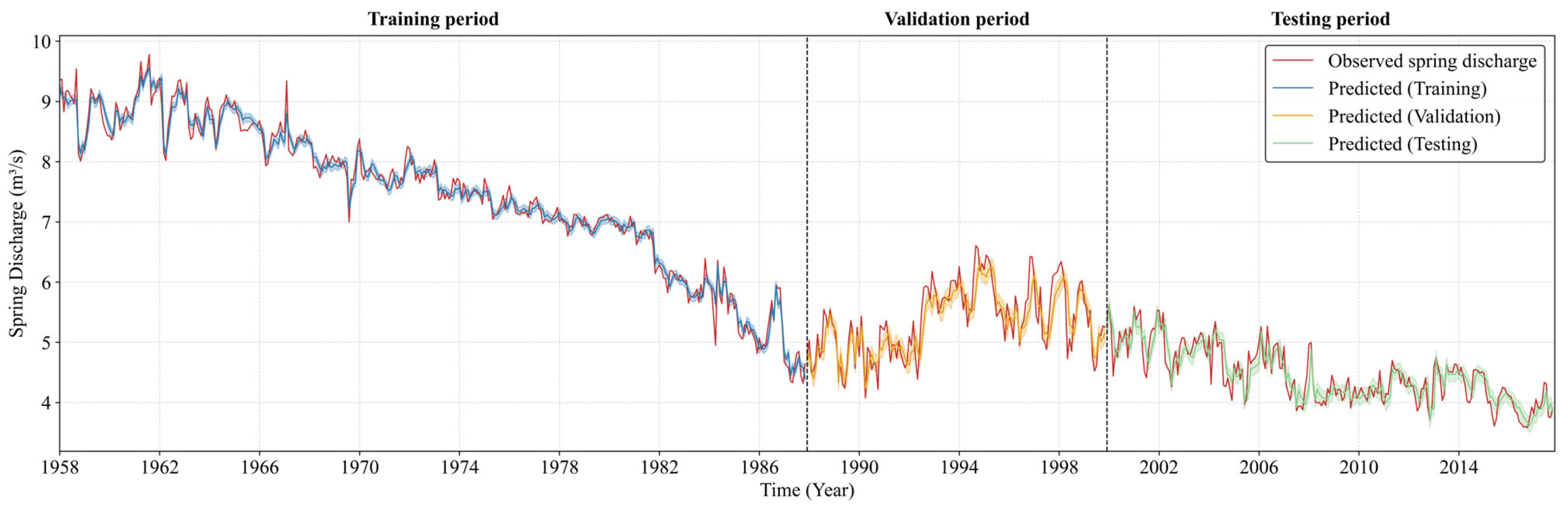
The dataset employed in this work comprises monthly records of precipitation and spring discharge extending from January 1958 through December 2020. To facilitate model development, the data were chronologically partitioned into three subsets: the period from 1958 to 1996 was designated as the training set, the interval from 1997 to 2008 was utilized for validation, and the observations from 2009 to 2020 were reserved for the test set.

The H-STGAT model was trained for 300 epochs using the Adam optimizer with an initial learning rate of 0.001. Training configurations included a Dropout rate of 0.2 and $L_2$ regularization (${\mathrm{w}\mathrm{e}\mathrm{i}\mathrm{g}\mathrm{h}\mathrm{t} \mathrm{d}\mathrm{e}\mathrm{c}\mathrm{a}\mathrm{y}=10}^{-4}$). Other hyperparameter settings and architectural configurations are specified in

Table 3. Model parameters setting.

Model Parameters	Values
$\mathrm{Lookback} \mathrm{Years} (K$)	5
$\mathrm{Temporal} \mathrm{Window} \mathrm{Size} (T$)	12
Number of H-STGAT Layers	2
$\mathrm{Hidden} \mathrm{Dimension} \mathrm{of} \mathrm{GAT} \left(d^{\mathrm{\prime }}\right)$	16
$\mathrm{Hidden} \mathrm{Dimension} \mathrm{of} \mathrm{MLP} \left(d_h\right)$	32
Loss function	MSE loss

Note: Lookback Years ($K$) represents the number of past years used to construct periodic patterns, Temporal Window Size ($T$) refers to the length of the recent consecutive monthly sequence used as input, Hidden Dimension of GAT ($d^{\mathrm{\prime }}$) is the feature dimension within the H-STGAT layers, and Hidden Dimension of MLP ($d_h$) indicates the dimension of the hidden layer in the final prediction network.

.

To quantify the potential variability in model outputs, an ensemble of 10 independent experimental runs was conducted using different random seeds for initialization. The final results are reported as the mean predictive values accompanied by a 95% confidence interval, which defines the estimated range of uncertainty for the discharge simulations. This probabilistic output provides a quantitative measure of the model’s prediction reliability for water resource management applications.

4.2. Effectiveness of Single-Step Spring Discharge Prediction

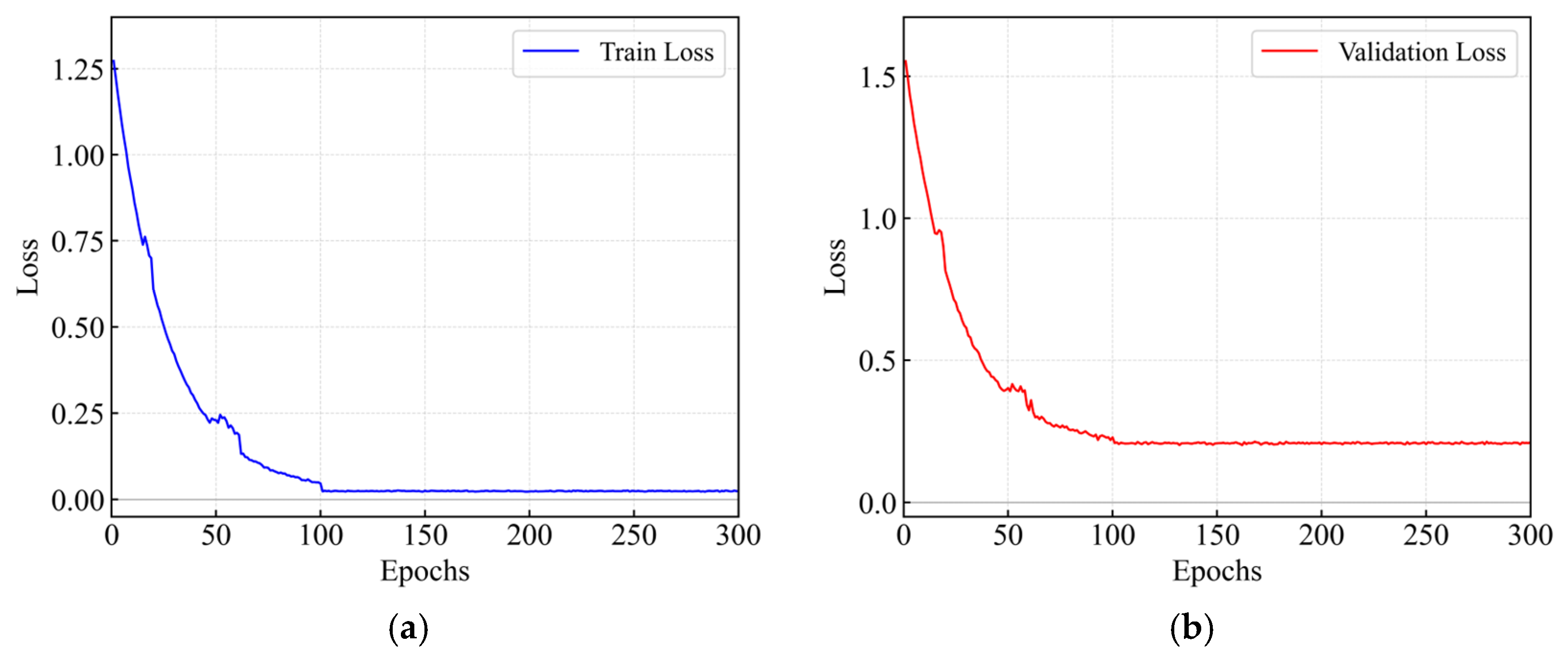
Figure 6 depicts the loss trajectories for both the training and validation phases. Initially, the two curves demonstrate a rapid and simultaneous decline, eventually reaching a steady state. Throughout the training duration, the gap between them remains negligible. This pattern of convergence serves as evidence of the model’s robustness and highlights the success of the applied regularization techniques in averting overfitting.

The trained model was employed to predict spring discharge for the ensuing month. To ensure statistical credibility, ten independent experiments were conducted with different random initializations.

Table 4. Performance metrics of single-step spring discharge prediction for the best-performing experiment among ten independent runs.

Performance Index	NSE	RMSE (m3/s)	MAE (m3/s)	MAPE (%)
Training period	0.9764	0.1900	0.1363	1.85
Validation period	0.7834	0.2676	0.2078	3.80
Testing period	0.7695	0.2261	0.1692	3.81

presents the resulting performance metrics, and Figure 7 visually compares the observed values with the single-step predictions. On the testing set, the model achieved a peak NSE of 0.7695 and an RMSE of 0.2261 m³/s. The 95% confidence interval is represented by the shaded area in Figure 7, confirming that the reported performance is a stable and reliable measure of the model’s predictive capability.

Performance differs between training and test sets due to distributional shifts in the long-term hydrological series: average spring discharge decreased from 6.92 m³/s (1958–1996) to 4.38 m³/s (2009–2020). The model maintained an NSE above 0.76 despite this non-stationarity, demonstrating its capacity to capture fundamental hydrological mechanisms.

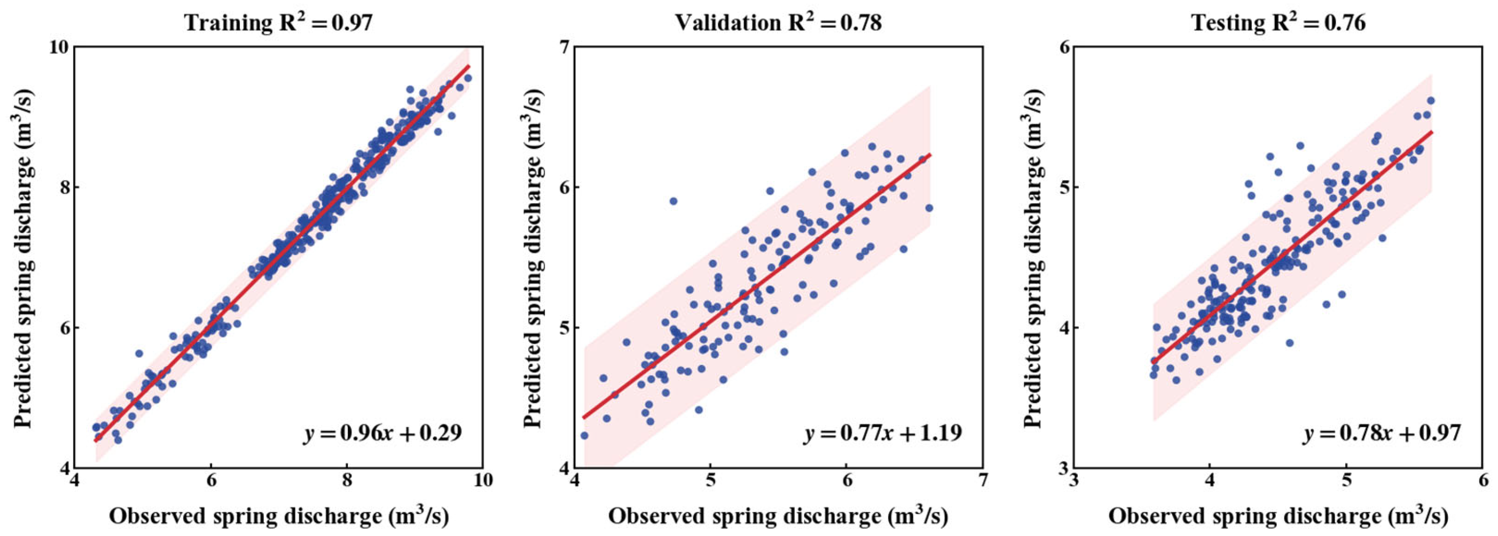
Figure 8 illustrates the scatter plots contrasting the observed versus predicted spring discharge across the training, validation, and testing stages. The model yielded $R^2$ scores of 0.97, 0.78, and 0.77 for the training, validation, and test datasets, respectively. Visually, the plots demonstrate that the majority of data points are tightly clustered along the 1:1 diagonal, indicating a strong alignment between the model predictions and actual measurements. Furthermore, the pink bands represent the 95% confidence intervals, defining the likely range of predictive variability. The narrowness of these intervals underscores the reliability of the forecasting results. In summary, the combination of high $R^2$ values and the dense concentration of scatter points corroborates the efficacy and robustness of the H-STGAT model for spring discharge prediction.

4.3. Effectiveness of Multi-Step Spring Discharge Prediction

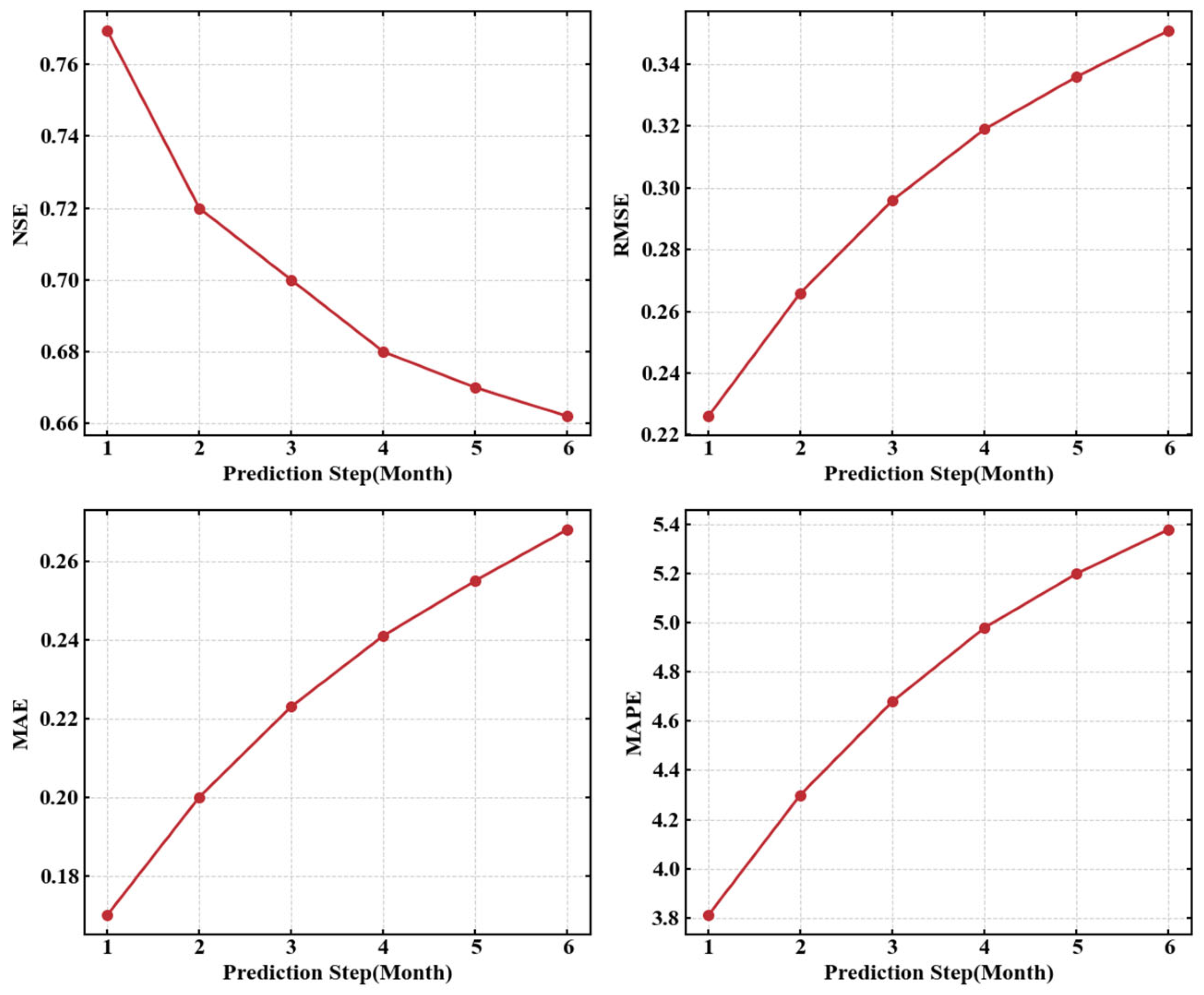
To evaluate the model’s long-term forecasting capability, we performed multi-step predictions for spring discharge up to six months ahead. As shown in Figure 9, the model’s performance (NSE, RMSE, MAE, MAPE) across these forecasting horizons is demonstrated on the test dataset.

Figure 9 displays the variations in the model’s predictive performance for spring discharge across forecast horizons ranging from 1 to 6 months. Overall, while a slight decline in accuracy is observed as the prediction horizon extends, the model’s performance remains acceptable. Specifically, for short-term forecasts of 1 to 3 months, the Nash–Sutcliffe Efficiency consistently exceeds 0.70, reaching 0.77 for the 1-month-ahead prediction, with RMSE and MAE values of 0.22 and 0.17 m³/s, respectively. This indicates the model’s effectiveness in capturing the variation patterns of spring discharge and reasonably representing the time-lag relationship between precipitation and groundwater recharge. When the forecast horizon is extended to 6 months, the NSE decreases to 0.67, while RMSE and MAE increase to 0.33 and 0.26 m³/s. Despite this decline, the model retains adequate trend-capturing ability, demonstrating robust long-term stability.

The observed decline in accuracy can be primarily attributed to the nonlinear storage and multi-scale response characteristics inherent to karst aquifer systems. Spring discharge is governed by the combined effects of precipitation infiltration, aquifer storage, and conduit flow. The precipitation signal attenuates during transmission, and its influence as an external driver diminishes over longer prediction horizons, while the delayed release effect from the groundwater system becomes more pronounced. Furthermore, increased forecast lead times introduce error accumulation, reducing the model’s sensitivity to local fluctuations. Overall, these findings reflect the typical mechanism of karst hydrologic systems characterized by “short-term response and long-term delayed release.”

5. Analysis and Discussion

5.1. Comparison with Other Baseline Models

To rigorously evaluate the predictive performance of the proposed H-STGAT model, a comparative analysis was conducted against a comprehensive set of benchmark models. These baselines encompass: (1) statistical models, specifically ARIMA [25] and MLR [26]; (2) ensemble learning, represented by XGBoost [27], recognized for its efficiency in capturing non-linear patterns in hydrological datasets; (3) recurrent and graph-based architectures, including GRU [28], LSTM [11], GCN [29], and GAT [21]; (4) the foundational Transformer [30] architecture and its frontier variants, namely Informer [13] and Autoformer [12], designed for capturing complex dependencies in long-sequence time-series.

To ensure the reproducibility of results and account for the stochastic nature of network initialization, all deep learning-based benchmarks were implemented under a unified experimental framework using standard configurations consistent with recent studies. Each model was subjected to 10 independent training iterations with distinct initialization seeds to verify training stability. The metrics reported in

Table 5. Performance Comparison of Various Models with Adaptive Multi-Timescale Fusion Data.

Model	NSE	MAE	RMSE	MAPE (%)
ARIMA	0.6207	0.2322	0.3094	5.236
MLR	0.6471	0.1733	0.2391	3.935
XGBoost	0.6514	0.1755	0.2368	4.102
GRU	0.6561	0.1853	0.2345	12.51
LSTM	0.6617	0.1841	0.2357	12.24
GCN	0.6718	0.2151	0.2741	4.431
GAT	0.6718	0.2151	0.2741	4.413
Transformer	0.7233	0.1887	0.2311	4.338
Informer	0.7425	0.1762	0.2294	3.955
Autoformer	0.7588	0.1710	0.2275	3.862
Ours	0.7695	0.1692	0.2261	3.810

Note: Bold values indicate the best performance in each column.

represent the optimal performance of the model selected based on the validation set, reflecting the peak capacity of each model for spring discharge forecasting.

As shown in Table 5, the results indicate that our proposed model achieved the best performance across all evaluation metrics among all the tested models. The traditional ARIMA and MLR models exhibit limited capability in capturing nonlinear hydrological dynamics, achieving relatively low Nash–Sutcliffe Efficiency values. While the tree-based XGBoost outperforms these statistical baselines, it lacks the mechanism to explicitly model the spatiotemporal connectivity between observation stations. Among deep learning approaches, GRU and LSTM models, which primarily focus on temporal dependencies, yield NSE values ranging from 0.65 to 0.67. Although GCN and GAT incorporate spatial correlations, their capacity to model long-term temporal relationships remains insufficient, resulting in NSE values of approximately 0.6718. The Transformer architecture and its advanced variants, such as Informer and Autoformer, leverage powerful attention mechanisms but often treat spatial variables as multivariate channels without incorporating the physical topology of the monitoring network. Consequently, they achieve improved but still suboptimal results compared to the proposed architecture.

This architecture enables the synergistic modeling of complex spatiotemporal lags and nonlinear interactions, encoding spatial proximity and periodic patterns directly into the learning framework. This is particularly well-suited to the characteristics of karst groundwater systems, including slow recharge-discharge dynamics and heterogeneous aquifer properties. Consequently, H-STGAT achieves a substantial improvement with an NSE of 0.7695, while also exhibiting significant reductions in RMSE, MAE, and MAPE. These findings verify the enhanced robustness and predictive accuracy of H-STGAT in simulating the nonlinear precipitation–discharge response, establishing it as a reliable predictive tool for the Shentou Spring catchment and offering a methodological reference for hydrological modeling in comparable karst systems.

5.2. Assessing the Contribution of Hydrological Relationships and Attention Mechanism

To validate the effectiveness of the key components in the proposed H-STGAT model, a series of ablation studies was conducted. These experiments evaluate the impact of removing specific hydrological relationships or attention mechanisms on the model’s performance. The results are summarized in

Table 6. Impact of key components on model performance, evaluated through an ablation study.

Model Variant (On the Test Set)	NSE	MAE	RMSE	MAPE (%)
w/o Spatial Hydro-relation	0.6441	0.2588	0.3407	6.335
w/o Hydrological Process Dependency	0.7153	0.2104	0.2915	5.021
w/o Hydrological Periodicity Pattern	0.4792	0.3198	0.4289	9.634
w/o Channel-wise Attention	0.7312	0.1995	0.2703	4.456
Full Model (H-STGAT)	0.7695	0.1692	0.2261	3.810

.

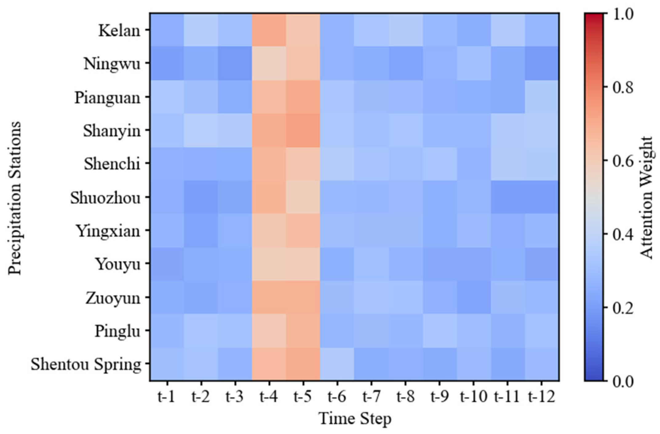
The results in Table 6 indicate that the complete H-STGAT model achieves the best performance across all evaluation metrics. Specifically, removing the Hydrological Periodicity Pattern leads to the most significant degradation in performance, with NSE dropping to 0.4792, highlighting that capturing the overall trend and seasonal variations serves as the essential framework for accurate spring discharge prediction. The ablation of Spatial Hydro-relation also results in substantial performance decline, underscoring that spring discharge is primarily driven by spatially distributed precipitation, and effective modeling of the spatial precipitation–discharge relationship significantly enhances simulation accuracy. Similarly, removing the hydrological process dependency causes notable deterioration, confirming the necessity of capturing the “memory” effects of hydrological processes. Furthermore, when the channel-wise attention mechanism is removed and replaced with simple averaging fusion, model performance also declines. This demonstrates that precipitation at different locations and time periods exerts varying influences on spring discharge. Precipitation exhibits spatially heterogeneous and temporally lagged effects on spring discharge, as illustrated in Figure 4. The attention mechanism in H-STGAT adaptively focuses on feature factors critical to spring discharge in a data-driven manner, thereby improving prediction accuracy. In summary, the ablation study validates that the three integrated hydrological relationships and the attention mechanism are all indispensable components. They operate synergistically to effectively enhance the model’s capability to simulate and predict complex karst hydrological processes.

5.3. Contribution Analysis of Feature Branches in a Hierarchical Attention Mechanism

The H-STGAT model extracts hydrological information from three channels: period, space, and time. The periodic channel reflects interannual variations and dominates the overall trend. The spatial channel reflects the spatial differences in recharge within the basin. And the temporal channel captures the dynamic responses of short-term processes. The model’s attention mechanism adaptively learns the importance weights of each channel. As shown in

Table 7. Attention Weight Allocation of Different Hydrological Features.

Dependency Relationships	Average Attention Weight
Periodic Dependency	0.653
Spatial Dependency	0.246
Temporal Dependency	0.101

, the weight of the periodic channel is the highest at 0.653, followed by the spatial channel at 0.246, and the temporal channel is the smallest at 0.101. This indicates that the model develops a prediction strategy of “trend-dominated, fluctuation-supplemented” during the learning process. The dominance of the periodic channel warrants merits particular attention. Although explicit variables for climate change and human activities are not direct inputs, the model effectively captures the cumulative impacts of these external stressors by assigning the highest weight to historical periodic patterns. Consequently, the H-STGAT architecture inherently accounts for the long-term trends driven by changing climatic conditions and anthropogenic interventions embedded within the multi-year hydrological time series.

Based on the ablation study results from the previous section, removing the periodic channel led to a 37.7% decrease in NSE, indicating its dominant role in establishing the baseline trend of spring discharge dynamics. This aligns with the hydrological understanding that karst springs exhibit strong seasonal patterns driven by annual precipitation cycles [1,14]. Removing the spatial channel resulted in a 16.3% decline in NSE and a 50.6% increase in RMSE, demonstrating that spatial heterogeneity of precipitation recharge is essential for capturing the distributed nature of karst aquifer systems. Eliminating the temporal channel caused a 7.0% drop in NSE, revealing that while short-term process memory contributes to refining predictions, its effect is relatively modest compared to trend and spatial components. When the adaptive attention mechanism was replaced with fixed equal weighting, NSE decreased by 5.0% to 0.7312, validating the effectiveness of learned adaptive weighting in multi-feature integration. These results demonstrate a hierarchical structure in karst spring discharge processes, where seasonal periodicity provides the fundamental framework, spatial precipitation patterns account for watershed-scale variability, and temporal process memory fine-tunes short-term dynamics. This hierarchical characterization provides valuable insights for understanding and modeling complex karst hydrological systems.

5.4. Identification of Spring Catchment Recharge Mechanisms Based on Spatial Attention Weights

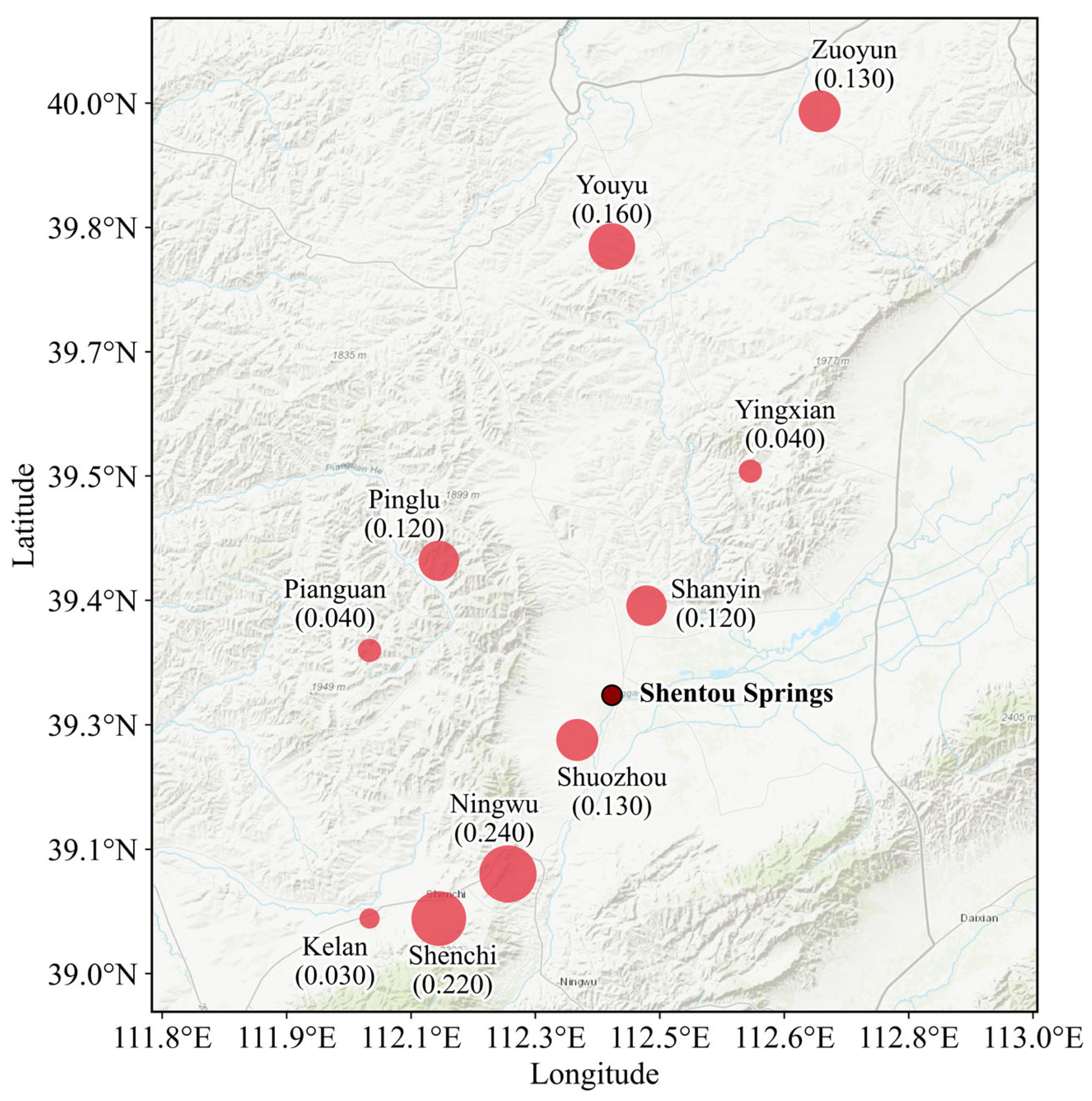
The H-STGAT model generates attention values within the spatial channel to quantify the spatial dependency strength among different stations, revealing the spatial intensity of information transmission. Figure 10 illustrates the spatial attention distribution learned by the model between ten precipitation stations and the spring discharge observation station, providing an intuitive depiction of the regional recharge relationships.

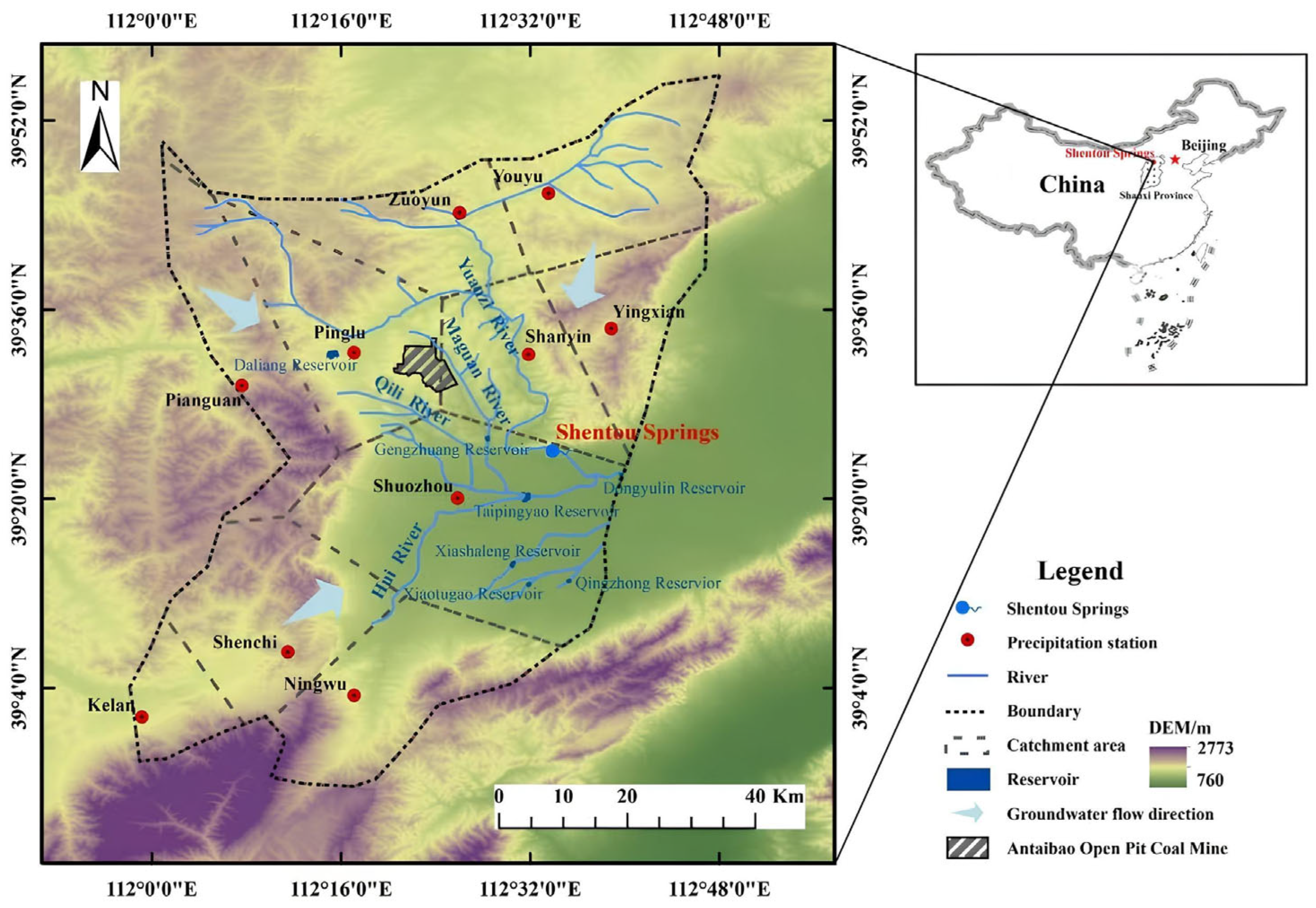
This distribution demonstrates a general consistency with the established hydrogeological conceptualization of the Shentou Spring Basin, offering empirical support for the model’s physical interpretability. Specifically, previous environmental tracer studies that utilizing stable (${}^{18}O$, $D$) and radioactive (${}^{87}\mathit{Sr}/{}^{86}\mathit{Sr}$) isotopes have explicitly identified the high-altitude carbonate outcrops of the Guancen Mountains as the principal recharge sources for the deep karst aquifer [18,19]. Aligning with this physical reality, the model autonomously assigned the highest attention weights of 0.24 and 0.22 to the Ningwu and Shenchi stations, respectively, which are situated within this core recharge zone. This convergence demonstrates that the H-STGAT model has correctly prioritized the dominant physical driving factors consistent with independent isotopic evidence.

Downgradient from the recharge zone, the model assigns intermediate weights of 0.16 and 0.13 to Youyu and Zuoyun, reflecting their hydrogeological function as lateral flow and transmission belts that facilitate groundwater transit. Conversely, basin margin sites such as Pinglu, Shuozhou, and Shanyin received lower weights ranging from 0.12 to 0.13, while peripheral stations like Kelan and Yingxian were assigned minimal importance of 0.03 and 0.04. This spatial attenuation corresponds to regional geological surveys [16,20], which indicate that these areas are characterized by thick quaternary sediment cover or act as discharge zones, thereby limiting their hydraulic connectivity to the deep karst system.

Collectively, this heterogeneous weight distribution—differentiating between distal recharge sources, transmission belts, and discharge areas—demonstrates that the H-STGAT model is capable of capturing spatial patterns that are largely consistent with the inherent recharge–flow–discharge mechanism. This suggests that the model can effectively approximate complex hydrogeological behaviors from spatiotemporal data without requiring explicit prior geological constraints.

5.5. Temporal Attention Mechanism for Capturing Dynamic Hydrological Process Memory

The temporal attention mechanism is designed to characterize the dynamic dependencies between consecutive time steps of precipitation and spring discharge. By constructing temporal edge connections between adjacent months, the model effectively captures the causal relationships and lagged response characteristics between precipitation and spring discharge. Figure 11 presents a visualization of this mechanism, including the distribution of attention values across different time steps and their average variation trend.

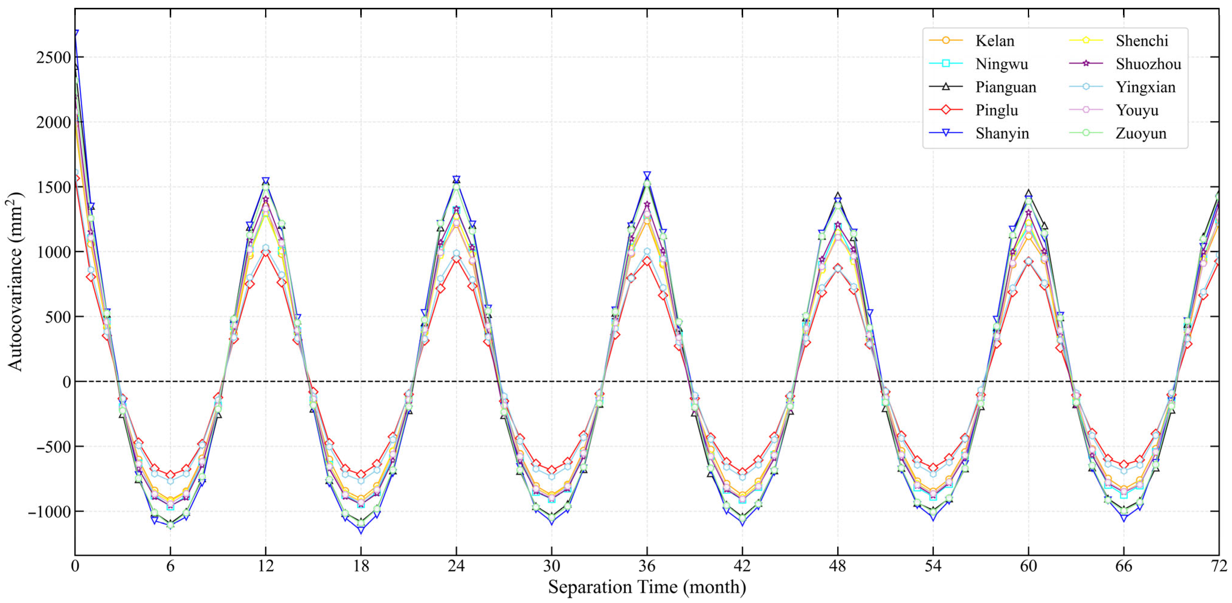
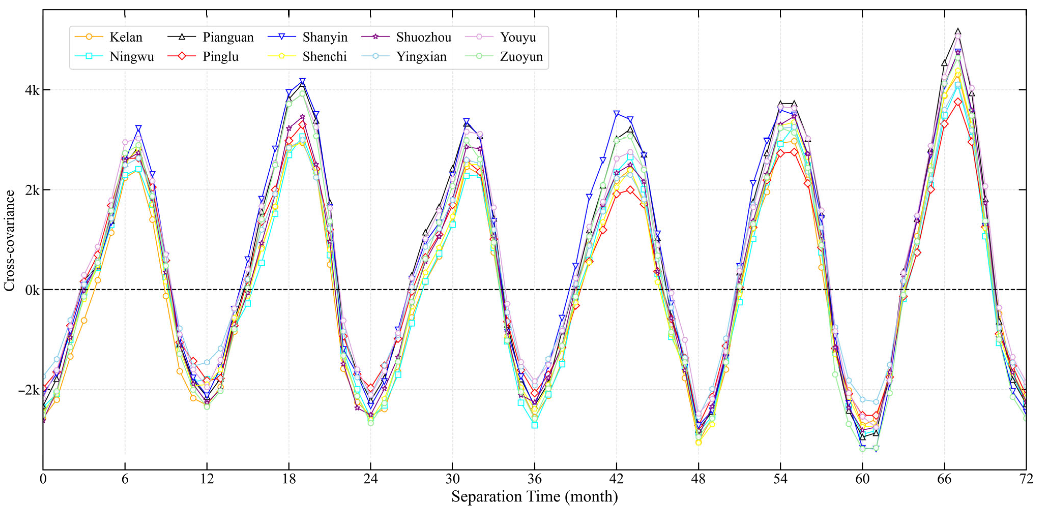
Figure 11 depicts the temporal attention characteristics of the precipitation–discharge relationship, visualizing the relative contribution of precipitation at different time steps to spring discharge prediction and its average trend. The results show that the model allocates the highest importance to inputs occurring 4 to 6 months prior to the current time step. This learned pattern mirrors the statistical lag identified in the cross-covariance analysis (Section 2.2). Such consistency suggests that the temporal attention mechanism effectively identifies the critical delay period associated with the aquifer’s storage–release processes. By autonomously focusing on these hydrologically relevant time windows, the model demonstrates an ability to align its predictive logic with the physical transit time of groundwater.

5.6. Historical Lookback Period Configuration

The H-STGAT model involves two critical temporal parameters: the Temporal Window Size (T) and the Lookback Years (K). The temporal window was set to T = 12 months based on hydrological principles, as a 12-month window represents a complete hydrological year that effectively captures seasonal variations and semi-annual lag effects. Unlike T, the optimal lookback period K lacks established theoretical guidance and depends on the trade-off between capturing interannual variability and avoiding information redundancy or computational burden. Therefore, we conducted experiments to determine the optimal K value by evaluating model performance under different historical data lengths ranging from 1 to 8 years.

Table 8. Performance of the H-STGAT model under different lookback period configurations.

Lookback Years (K)	Model Size (KB)	NSE	MAE	RMSE	MAPE (%)
1	745	0.718	0.195	0.248	4.38
2	1180	0.738	0.184	0.239	4.12
3	1625	0.755	0.176	0.231	3.95
4	2315	0.761	0.171	0.227	3.84
5	3028	0.769	0.170	0.226	3.81
6	4095	0.758	0.177	0.230	3.97
7	5195	0.743	0.185	0.237	4.15
8	6520	0.726	0.193	0.245	4.33

Note: The row in bold indicates the optimal lookback period configuration ($K=5$) selected for the final model.

presents the experimental results under different lookback period configurations with T fixed at 12 months.

The results indicate that model performance initially improves with increasing historical length, reaching optimal performance at K = 5 years with an NSE of 0.769, RMSE of 0.226 m³/s, MAE of 0.170 m³/s, and MAPE of 3.81%. This suggests that a five-year historical period effectively captures interannual variability and multi-year climate oscillations without introducing excessive noise from outdated information. When K exceeds 5 years, model accuracy gradually declines, with NSE dropping to 0.726 at K = 8, indicating that excessively long historical inputs introduce outdated hydrological information that weakens the model’s sensitivity to current conditions. Meanwhile, model size expands rapidly from 745 KB at K = 1 to 6520 KB at K = 8, leading to a sharp rise in computational and storage demands. Overall, the combination of T = 12 months and K = 5 years provides the best balance between predictive accuracy and computational efficiency, making it the optimal configuration for the H-STGAT model in this study.

6. Conclusions

This study proposes the H-STGAT for karst spring discharge prediction. Experimental results demonstrate that H-STGAT outperforms traditional baselines, achieving a Nash–Sutcliffe Efficiency of 0.77 and a Root Mean Square Error of 0.22 m³/s. The main conclusions are as follows:

(1)

By introducing a heterogeneous graph modeling structure, the model jointly embeds recent observational data and same-month data from previous years as nodes in the graph. Utilizing spatial connection edges, temporal dependency edges, and cross-year same-month connection edges, it uniformly characterizes the multi-dimensional hydrological relationships within the catchment. In the context of karst hydrological system modeling, the proposed structure exhibits collaborative modeling capability for complex spatial, temporal, and periodic features, outperforming single-scale models.

(2)

The model employs a dual-layer graph attention mechanism. At the node level, hydrological features are extracted separately through spatial, temporal, and periodic channels, while at the channel level, adaptive fusion of multi-relational features is achieved via weight learning, thereby substantially improving the model’s capacity to identify critical hydrological drivers. Quantitative analysis reveals that the periodic channel with a dominant weight of 0.653 governs the primary trend framework, whereas the spatial and temporal channels, weighted at 0.246 and 0.101, respectively, serve to resolve localized heterogeneity and short-term fluctuations.

(3)

The interpretability analysis validates the physical consistency of the model. At the spatial level, the attention mechanism effectively identifies the primary recharge areas by assigning the highest contribution shares of 22% to 24% to the Ningwu and Shenchi stations, consistent with independent isotope studies. At the temporal level, it reveals a lagged response characteristic of approximately 4 to 6 months between precipitation and spring discharge, matching the inherent statistical properties of the catchment. This alignment confirms the model’s reliability in both physical interpretability and predictive capability.

The H-STGAT model achieves multi-channel modeling within a unified framework, offering a novel approach for spatiotemporal prediction in karst hydrological systems. Future work will focus on the model’s transferability and real-time prediction capabilities, while integrating climate change and anthropogenic factors to further support sustainable water resource management and ecological conservation.