Article

Sustainable Safety Planning on Two-Lane Highways: A Random Forest Approach for Crash Prediction and Resource Allocation
by
Fahmida Rahman
1,*,
Cidambi Srinivasan
2,
Xu Zhang
3 and
Mei Chen
4,*
1
Department of Civil and Environmental Engineering, Rowan University, Glassboro, NJ 08028, USA
2
Dr. Bing Zhang Department of Statistics, University of Kentucky, Lexington, KY 40506, USA
3
Kentucky Transportation Center, University of Kentucky, Lexington, KY 40506, USA
4
Department of Civil Engineering, University of Kentucky, Lexington, KY 40506, USA
*
Authors to whom correspondence should be addressed.
Sustainability 2026, 18(2), 635; https://doi.org/10.3390/su18020635
Submission received: 25 September 2025 / Revised: 22 November 2025 / Accepted: 30 December 2025 / Published: 8 January 2026
(This article belongs to the Special Issue Sustainable Urban Mobility: Road Safety and Traffic Engineering)

Abstract

During the safety planning stage, accurate crash prediction tools are critical for prioritizing countermeasures and allocating resources effectively. Traditional statistical approaches, while long applied in this field, often depend on distributional assumptions that may introduce bias and limit model accuracy. To address these issues, studies have started exploring Machine Learning (ML)-based techniques for crash prediction, particularly for higher functional class roads. However, the application of ML models on two-lane highways remains relatively limited. This study aims to develop an approach to integrate traffic, geometric, and critically, speed-based factors in crash prediction using Random Forest (RF) and SHapley Additive exPlanations (SHAP) techniques. Comparative analysis shows that the RF model improves crash prediction accuracy by up to 25% over the traditional Zero-Inflated Negative Binomial model. SHAP analysis identified AADT, segment length, and average speed as the three most influential predictors of crash frequency, with speed emerging as a key operational factor alongside traditional exposure measures. The strong influence of speed in the RF–SHAP results depicts its critical role in the safety performance of two-lane highways and highlights the value of incorporating detailed operating characteristics into crash prediction models. Overall, the proposed RF–SHAP framework advances roadway safety assessment by offering both predictive accuracy and interpretability, allowing agencies to identify high-impact factors, prioritize countermeasures, and direct resources more efficiently. In doing so, the approach supports sustainable safety management by enabling evidence-based investments, promoting optimal use of limited transportation funds, and contributing to safer, more resilient mobility systems.

1. Introduction

The importance of reliable crash prediction tools has grown as transportation agencies increasingly emphasize proactive and sustainable road safety management. Sustainable safety planning requires not only reducing crashes but also ensuring that investments are targeted, efficient, and aligned with broader sustainability goals such as minimizing future system-wide risk, optimizing limited public resources, and improving long-term mobility outcomes. In support of these goals, agencies now place greater emphasis on robust quantitative methods during the early planning stage [1,2]. This has been evident in their collaborative efforts to improve overall roadway safety. In line with this, the American Association of State Highway and Transportation Officials (AASHTO) underscored the significance of advanced statistical quantitative analyses by publishing the Highway Safety Manual (HSM) in 2010 [3]. The HSM provided the first comprehensive model to predict both crash frequency and severity based on traffic, roadway, and roadside characteristics [3]. Agencies rely on this quantitative technique to assess the potential safety implications of various design alternatives and forecast potential scenarios [4].
The HSM approach consists of three key elements: base safety performance functions (SPFs), crash modification factors (CMFs), and calibration factors [3,5]. SPFs are statistical models that are utilized to predict crash frequency on a road under standard conditions [5]. These SPFs are then adjusted using CMFs and calibration factors to account for non-base conditions and local jurisdictions. Similar to any statistical model, SPFs determine the relationship between explanatory variables (e.g., roadway and traffic attributes) and the response variable (e.g., crash frequency) based on their functional form and coefficients. However, statistical models encounter several issues that can limit the application of SPFs [6,7,8]. First, the analysts need to assume the probability distribution of the crash data. Furthermore, statistical models require the assumption of a predefined functional form and the estimation of fixed parameters, which can lead to biased results. Moreover, the association among independent variables is often overlooked, thereby affecting the overall adequacy of the model. In addition, these models have been criticized in the existing literature for their low predictive accuracy [6].
Machine learning (ML) methods, on the other hand, have received attention as an alternative to traditional regression models due to their ability to address the underlying issues in traditional models. These non-parametric techniques require no prior assumptions about the distribution of crash data and can identify complex, non-linear relationships between a response variable and multiple independent variables while achieving high prediction accuracy. In particular, ML models have shown satisfactory performance in crash prediction when compared to traditional statistical models [7,9,10,11,12,13,14,15]. However, there have been concerns regarding the practical applicability of ML models due to their lack of interpretability and black-box nature. To address this, researchers have started adopting various interpretation methods, for example, Partial Dependence Plots (PDP), Local Interpretable Model-agnostic Explanations (LIME), SHapley Additive exPlanations (SHAP), and Local Sensitivity Analysis (LSA) [10,11,16,17]. These models have been applied to understand the relationship between the model outcomes and the independent variables.
Past research has predominantly examined the effectiveness of ML models in predicting crash frequencies on freeways, multilane highways, arterials, and urban and suburban roads [9,10,11,14,15,16]. These studies also explored the effect of different explanatory variables on crashes based on ML model results. However, the application of machine learning models for predicting crashes and evaluating the effects of various factors on ML model outcomes in the context of two-lane highways remains relatively limited. We attempt to fill this gap in the current study.
In this study, we applied an RF-based model to analyze crash frequency on two-lane highways in Kentucky, which comprise approximately 88.7% of the total state-maintained centerline mileage and account for nearly half of all roadway crashes. The objective was to demonstrate an integrated methodological approach for combining crash data with speed, roadway geometry, and traffic conditions to uncover the underlying factors associated with crash frequency. To assess the predictive capability, the RF model was compared with the traditional zero-inflated negative binomial (ZINB) model. Furthermore, the outcomes of the RF model were analyzed using the SHAP method to gain valuable insights into the relationships between explanatory variables and crash frequency. Beyond enhancing prediction accuracy, the RF–SHAP framework is extended into an applied decision support tool, demonstrating how agencies can incorporate interpretable ML outputs into prioritizing countermeasures and allocating safety resources in a more sustainable and data-informed manner.
The structure of the rest of the paper is as follows: In the next section, we provide a summary of the traditional and machine learning methods utilized in the existing literature on crash modeling. After that, the paper outlines the data sources used in this study and the preprocessing steps undertaken to ensure the data quality. Later, we present the two main methodologies used to achieve our research objective: the ZINB and RF models. The performance comparison of these models in predicting crash frequencies on two-lane highways is presented in the Section 5. This section also includes the interpretation of the results obtained from the RF model, highlighting the most influential factors contributing to crash occurrences. After that, we demonstrate the application of the framework for project prioritization and resource allocation in Section 6. Lastly, we provide a comprehensive summary of our findings and conclusions in Section 7. Additionally, we discuss potential areas for future research and further advancements in the field of modeling crashes for two-lane highways in Section 8.

2. Literature Review

Research has focused on understanding the relationship between crash frequency and its influencing factors, with the goal of developing analytical tools for more accurate crash prediction. Count models like Poisson, Negative Binomial (NB), Zero Inflation based-Poisson, and NB have been popular among the analytical tools used for estimating crash frequencies and assessing relevant factors [18,19,20,21,22,23,24,25,26,27,28,29]. Alternative modeling approaches, including but not limited to least-square linear regression, multivariate models, and random effect parameter models, have also been utilized in the analysis of crashes [30,31,32,33,34,35]. Furthermore, practitioners have started using spatial modeling tools to investigate the localized effects of crash predictors and suggest safety improvement plans for certain regions [36,37,38,39,40,41]. While these traditional statistical modeling approaches offer interpretability and model transferability, they may face challenges due to their reliance on assumptions about the distribution of crash data and the functional form used in model development [42]. When these assumptions are violated, it can lead to inaccurate predictions or misinterpretations of the related factors [43].
Machine learning models have gained popularity for addressing the limitations of traditional statistical models and have shown improved performance in crash prediction. For instance, Zeng et al. demonstrated the potential of a neural network (NN) model for predicting crash frequency on roadways in Hong Kong, achieving enhanced predictive performance compared with the traditional NB model [12]. Similarly, Yu et al. adopted a support vector machine (SVM) method to evaluate the crash risk of freeways in real time, which outperformed logistic regression models [14]. In another study, SVM proved to be a reliable network screening tool for urban signalized and unsignalized intersections, achieving better results than the NB model [15]. Additionally, the same study examined the predictive power of the RF approach for network screening and reported results that were promising compared to those of the NB model. Further evidence of the effectiveness of the RF-based approach came from a study by Pu et al., which employed an RF model to explore the non-linear relationship between vertical curve features and crash frequency on interstate highways [10]. In their study, the RF model outperformed the traditional random effect negative binomial (RENB) model. Moreover, Das et al. highlighted the better capability of RF in predicting run-off-road crashes on two-lane roads compared to the NB model [13]. The RF model was also applied to predict freeway crashes and was found to outperform several models, including logistic regression, support vector machines, and extreme gradient boosting [44].
Although ML models have demonstrated reasonable prediction accuracy in the existing traffic safety literature, their application remains questionable due to difficulties in interpreting model outputs and in uncovering relationships between risk factors and model outputs. To address this issue, studies started to adopt interpretation methods such as PDP, SHAP, LIME, LSA, etc. These methods offer valuable insights into the complex impacts of risk factors on crash occurrences. For instance, Saha et al. applied PDP in order to investigate the marginal impact of contributing variables on crash predictions [16]. They did this by leveraging results from the boosted regression trees (BRT) model, developed for urban and suburban facility types and arterials. Similarly, Pu et al. employed PDP to interpret results from an RF model for crash frequency on vertical curves of interstates [10]. In another context, Yu and Abdel-Aty performed a sensitivity analysis using LSA to investigate the relationships between explanatory variables and crash severity injuries on freeways based on an SVM model [45]. Wei et al. applied SHAP to interpret the results of XGBoost and examine the primary and interaction effects of risk factors on short-duration crashes on two-lane highways [17]. Wen et al. conducted a comprehensive evaluation of LIME, PDP, LSA, and SHAP for interpreting results from different ML models used for run-off-road crashes on highways [11]. SHAP provides global feature importances by averaging SHAP values across individual predictions. For local interpretability, SHAP assigns each feature a contribution value for an individual prediction, which can be used to visualize the local effects and interactions of features through dependence plots [46]. Another example of interpreting ML models is Variance-based Global Sensitivity Analysis (GSA) which ranks explanatory variables, screens negligible factors, offers global interpretability, and identifies the overall contribution of each variable across the entire input space [47,48].
In summary, existing studies have highlighted improvements in crash prediction using ML models over traditional approaches. However, most studies focused on freeways, urban intersections, and arterials, with little attention to two-lane highways. This is due to limited data availability on two-lane highways. As more data become available on these roads through the advanced techniques, our study aims to develop a crash prediction model specific to these roads using the RF regression technique. To enhance model interpretability, we incorporated the SHAP method, which helps explain model results and provides insights into the key factors affecting crash frequency.

3. Data Collection & Processing

Data were collected for the two-lane highways in Kentucky. Crash data pertaining to the period from 2013 to 2017 were extracted from the Kentucky State Police database. The Highway Information System (HIS) (https://transportation.ky.gov/Planning/Pages/Centerlines.aspx, accessed on 1 January 2019) of the Kentucky Transportation Cabinet (KYTC) provided various roadway features, including traffic volume, lane width, shoulder types, shoulder width, curvature, grades, functional classifications, etc. These attributes facilitated the segmentation of roads into homogeneous sections, and crashes were linked to their respective segments [49]. However, we did not include any crash records that occurred within 100 ft. of intersections since a different set of factors contributes to such crashes. This buffer distance follows the internal practices of the Kentucky Transportation Center (KTC) for maintaining the statewide intersection database [50]. Additionally, segments shorter than 0.1 miles were also excluded based on the findings of Hauer and Bamfo [51].
To include speed-related factors in the analysis, GPS-based probe speed data were collected for 2015–2017 from HERE Technologies [52]. Whenever probes were observed on two-lane highways, these data were available at intervals of five minutes for each day, and they were available in both directions. The speeds were referenced to the HERE road network, which was then combined with the homogeneous segments to establish a spatial connection between the speed, the roadway characteristics, and the crash-related dataset. The conflation was performed following the methodological framework developed by Xu and Chen [53]. The framework uses intersection and link-sequence correspondences to preserve directional consistency and applies fuzzy logic to handle network uncertainties. Through this process, each HERE link was matched with the corresponding road segment with high spatial accuracy.
Later, to ensure that only segments with sufficient data were used in the analysis, a data adequacy check was conducted. We followed the approach proposed by Li et al. to determine the minimum sample size for speed data for each roadway segment [54]. Such method has been utilized to determine an appropriate sample size for the gathered traffic data, taking into consideration the dispersion of the data, in order to ensure that it falls within an acceptable margin of error [54,55].
By comparing the estimated minimum sample sizes corresponding to each segment with the available speed data, this study exclusively included segments that fulfilled the minimum sample size requirement. An exploratory assessment revealed that nighttime observations were extremely sparse across the network, approximately 50% of segments had less than 2% nighttime coverage, and the median nighttime availability was only 1.54%, compared to 14% during daytime. Even at the 75th percentile, nighttime coverage reached only 4.99%, whereas daytime coverage exceeded 33%. Since reliable estimation of segment-level aggregated speed requires sufficient temporal sampling, this study utilized the daytime speeds (from 6 am to 8 pm). After these pre-processing steps, the dataset comprised 49,776 segments, covering 13,133 miles in Kentucky. Figure 1 shows the map with the two-lane segments considered for this study.

4. Methodology

In this study, a random forest regression approach was employed to predict crash frequencies on two-lane highways. To assess the performance of the developed model relative to traditional methods, a ZINB model was adopted as the baseline model. In this section, we focus on discussing the underlying methodology of the RF model.
The random forest method is extensively employed in the field of supervised learning for classification and regression purposes. The non-parametric method possesses the ability to effectively capture complex non-linear associations between explanatory factors and the output of the model. It was introduced by Breiman in 2001 [56]. The RF algorithm utilizes an ensemble approach based on decision trees. The construction of each decision tree within the ensemble involves the utilization of numerous bootstrap training samples. This process involves the random selection, with replacement, of data points from the original population. The bootstrapping approach creates varied training sets for each tree, ensuring that the ensemble spans a broad spectrum of events. This helps reduce the risk of overfitting, leading to more accurate predictions [57].
When it comes to generating predictions, the RF model aggregates the outputs from all individual trees. Each tree independently provides predictions for the testing data, and the final prediction is obtained by averaging these outputs. A subset of the explanatory variables is utilized by the RF model to split each node within each decision tree. This step is taken to prevent any correlation between individual trees. To determine the ideal split point for each node, a splitting algorithm is applied to the subset of the selected explanatory variables, and then the results are determined. The objective of the splitting method is to achieve the highest possible level of homogeneity inside each consecutive node at a certain value of a chosen variable.
The RF model offers several advantages. One notable strength of this approach is its ability to adapt to varied data patterns and handle complex relationships among variables without the need for any predefined functional form [56,58]. Additionally, the RF model can address multicollinearity issues [56]. Moreover, it provides valuable insights into the importance of variables, indicating their respective contributions to the model predictions [56,58].
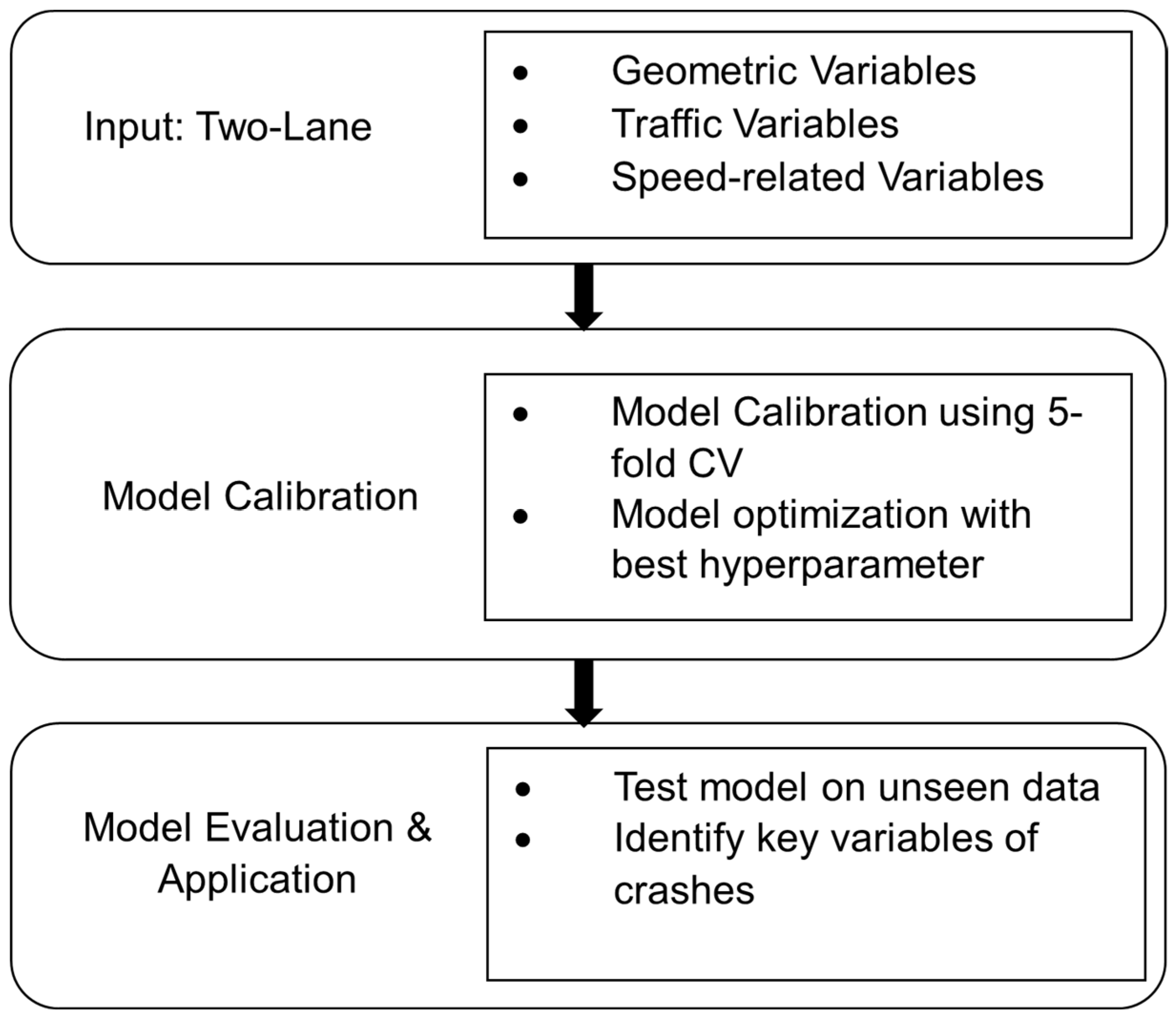
In this study, the RF model was utilized to identify the factors of the crash frequencies. The overall workflow for applying the RF model in crash analysis is illustrated in Figure 2. The process begins with inputting the selected geometric, traffic, and speed-related variables, followed by model calibration and performance evaluation. The following section provides a detailed description of each step in the modeling process.

5. Analysis & Results

5.1. Variable Selection

To develop an RF regression model for predicting crash frequencies on two-lane highways, we utilized a set of explanatory variables consisting of geometric, traffic, and speed characteristics associated with these highway segments. Statistics related to these characteristics are presented in Table 1. The geometric characteristics of segments include segment length, curvature, lane width, and shoulder width. On the other hand, speed-related characteristics of these segments are represented by average speed, the 85th percentile speed, and the standard deviation (std) of speed, which were combined from both directions of a segment. Furthermore, the table presents the statistical summary for the total crash frequencies during the five years. The crashes were summed up from both directions of the road.
Notably, some segments in the dataset exhibit a low average speed. The presence of very restrictive geometric constraints, such as narrow lanes and sharp curves, is the primary cause of this low average speed. In addition, it is important to note that several study segments have average or 85th percentile speeds that are well below the conventional speed limit of 88.5 kmph (55 mph) for two-lane roads in Kentucky. Once again, this is because of the limited geometric characteristics of these segments.
To ensure the final set of explanatory variables used for the RF model was not highly correlated, a thorough correlation analysis was conducted. The Pearson correlation coefficient (PCC) was employed to evaluate the high correlation between the variables. Typically, a PCC value greater than 0.5 indicates a strong correlation between two variables [59]. However, following the approach by Wei et al., we decided to increase the threshold for high correlation to 0.8 [17]. This decision was motivated by the fact that decision tree-based approaches, for instance, RF, tend to be very robust to multicollinearity among variables [17]. Based on this criterion, the 85th percentile speed was removed from the model due to its high correlation with the average speed.

5.2. Random Forest Calibration

To calibrate the RF model, we randomly split the dataset into two sets: a training set containing 70% of the data and a test set containing the remaining 30%. The calibration process involved adjusting a set of hyperparameters to achieve a balance between high prediction accuracy and low overfitting or underfitting in the trained model. We considered five hyperparameters, as presented in Table 2, for the calibration process. The selection of these specific hyperparameters was based on existing studies [60,61,62,63].
Each hyperparameter has its own significance in the predictions from model. For example, the accuracy of a model can be enhanced by raising the value of n_estimators. Nevertheless, beyond a certain threshold, further increments in n_estimators may no longer have a significant impact on the accuracy. In accordance with the methodology proposed by Saha et al., we selected the values of 500, 1000, 5000, and 10,000 for the parameter n_estimators [64]. As recommended by Genuer et al., we experimented with p   and p as values for the max_features parameter in low-dimensional regression situations [65]. Another crucial hyperparameter, Max_depth, was also considered, as continuous increases in max_depth can lead to overfitting issues. We explored different values for max_depth, as outlined in Table 2. We also considered the parameters min_samples_leaf and min_sample_split to further reduce the likelihood of overfitting. These hyperparameters regulate tree growth, thereby mitigating overfitting to the training data. It is possible that the construction of the largest tree will occur when these hyperparameters are set to their minimum possible values. As a result, in addition to the default values of 1 and 2, which are shown in Table 2, different values were investigated for the min_samples_leaf and min_sample_split parameters.
The procedure for determining the optimal hyperparameter combination for the RF model involved using the Python 3.10.16 package ‘RandomizedSearchCV’. This package automates the entire search process by incorporating cross-validation (CV) to identify the best combination. The aforementioned procedure facilitated the construction of several models, each employing distinct hyperparameter combinations, and subsequently assessed their performance using CV. For this study, we utilized a 5-fold CV methodology to assess the performance of each model and mitigate the issue of overfitting. The dataset was separated into five stratified portions using the 5-fold CV. Sequentially, each portion was utilized as the designated dataset for testing purposes, while the rest of the data were allocated as the training set. The Mean Squared Error (MSE) was computed for each fold using Equation (1) and subsequently averaged across five folds. The 5-fold CV procedure was iterated for the models using various combinations of hyperparameters, and the average MSE was computed for each model. Finally, after evaluating the model that produced the lowest MSE, we determined the optimal set of hyperparameters. The optimal hyperparameter values are shown in Table 2.
M S E = 1 n i   ϵ   t e s t i n g   d a t a n ( y i   y ^ i ) 2
where yi is the actual crash frequency for the ith observation in the testing data, y ^ i is the predicted crash frequency for the ith observation in the testing data, and n is the size of the testing dataset.

5.3. Performance Evaluation

After identifying the optimal hyperparameter combination, we developed the RF model using those hyperparameters. To evaluate its performance, we compared the RF model against a baseline model, which is ZINB in this case. Approximately 55% of the study segments reported zero crashes, suggesting potential overdispersion due to excess zeros. To account for this, we employed ZINB [26,66,67,68,69]. The selection of the ZINB model was further supported by prior studies by Rahman and Rahman et al., which demonstrated the benefits of the ZINB method in a similar context [63,70]. Additional methodological details can be found in these studies.
As performance measures, R2, Root Mean Squared Error (RMSE), and Mean Absolute Deviation (MAD), shown in Equations (2)–(4), are utilized.
R 2 = 1 i = 1 n ( y i y i ^ ) 2 i = 1 n ( y i y ¯ ) 2
R M S E = i = 1 n ( y i y i ^ ) 2 n
M A D = i = 1 n y i y i ^ n
where yi is the actual crash frequency, y i ^ is predicted crash frequencies, y ¯ is the mean of actual crash frequencies, and n is the number of segments.
Table 3 shows the predictive performance of both the RF and ZINB models, assessed on separate training and test datasets. It is worth noting that the traditional ZINB model can be sensitive to multicollinearity, and including highly multicollinear variables can lead to unreliable results. Therefore, we identified high multicollinearity (PCC higher than 0.5) among the explanatory variables and excluded them from the ZINB model. The final ZINB model was developed with AADT, length, average speed, and curvature, as presented in Equation (5). The comparison between RF and ZINB models clearly indicates that RF outperformed the ZINB model. By capturing the non-linear relationship between the contributing factors and the crash frequencies, the RF model significantly improved its predictive performance, with the maximum improvement being around 25% when considering the testing dataset.
μ = e 4.445 + 0.865   L n A A D T + 0.907 L n l 0.009 v a + 0.041 c u    
where μ is the mean crash frequency in 5 years, AADT is the annual average daily traffic, l is the segment length, va is the average speed, and cu is the roadway curvature.
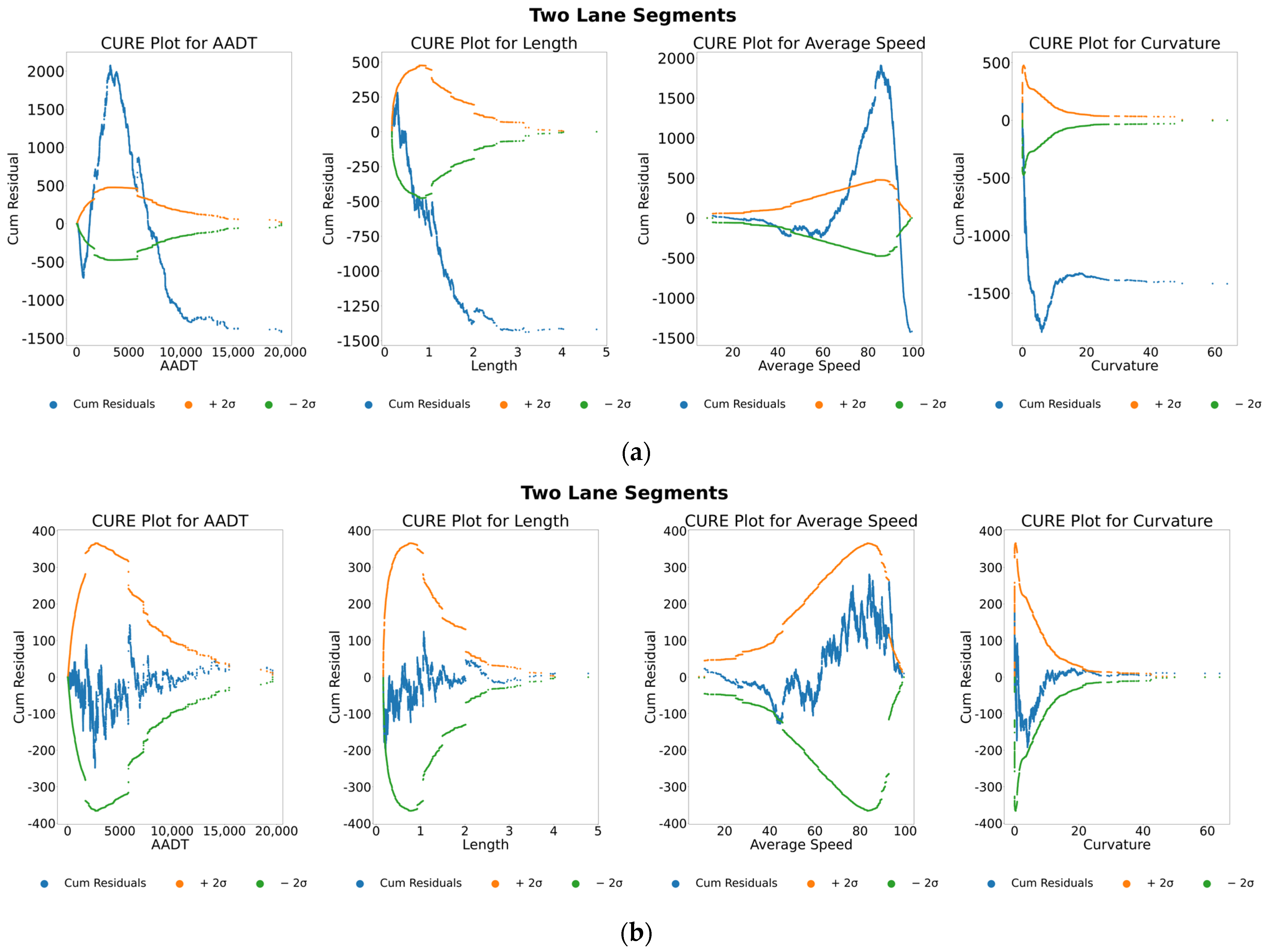
To conduct a more comprehensive comparison of the model fits between the RF and ZINB models, we also looked at cumulative residual (CURE) plots. These plots were constructed by arranging the cumulative residuals, which denote the difference between the observed and estimated crash counts from the model, in ascending order for each explanatory variable [51]. A random walk technique was used to evaluate the CUREs within a 95% confidence interval (CI). A model is deemed to be a good-fit model if its cumulative residual curve remains within two standard deviations ( ± 2 σ ) for 95% of the time [51].
Figure 3a,b display the CURE plots for AADT, segment length, average speed, and curvature, which were used in both RF and ZINB models. Upon examination, it becomes evident that the ZINB model does not adequately fit the observed data, as a substantial proportion of the CURE lies outside the ±2σ boundary for each variable. In contrast, for each variable, the CURE plots for the RF model show that a significant portion of the CURE is contained inside the ±2σ boundary, suggesting that the RF model exhibits a much better fit to the observed data in comparison to the ZINB model. This shows the effectiveness of the RF model for robust crash prediction.
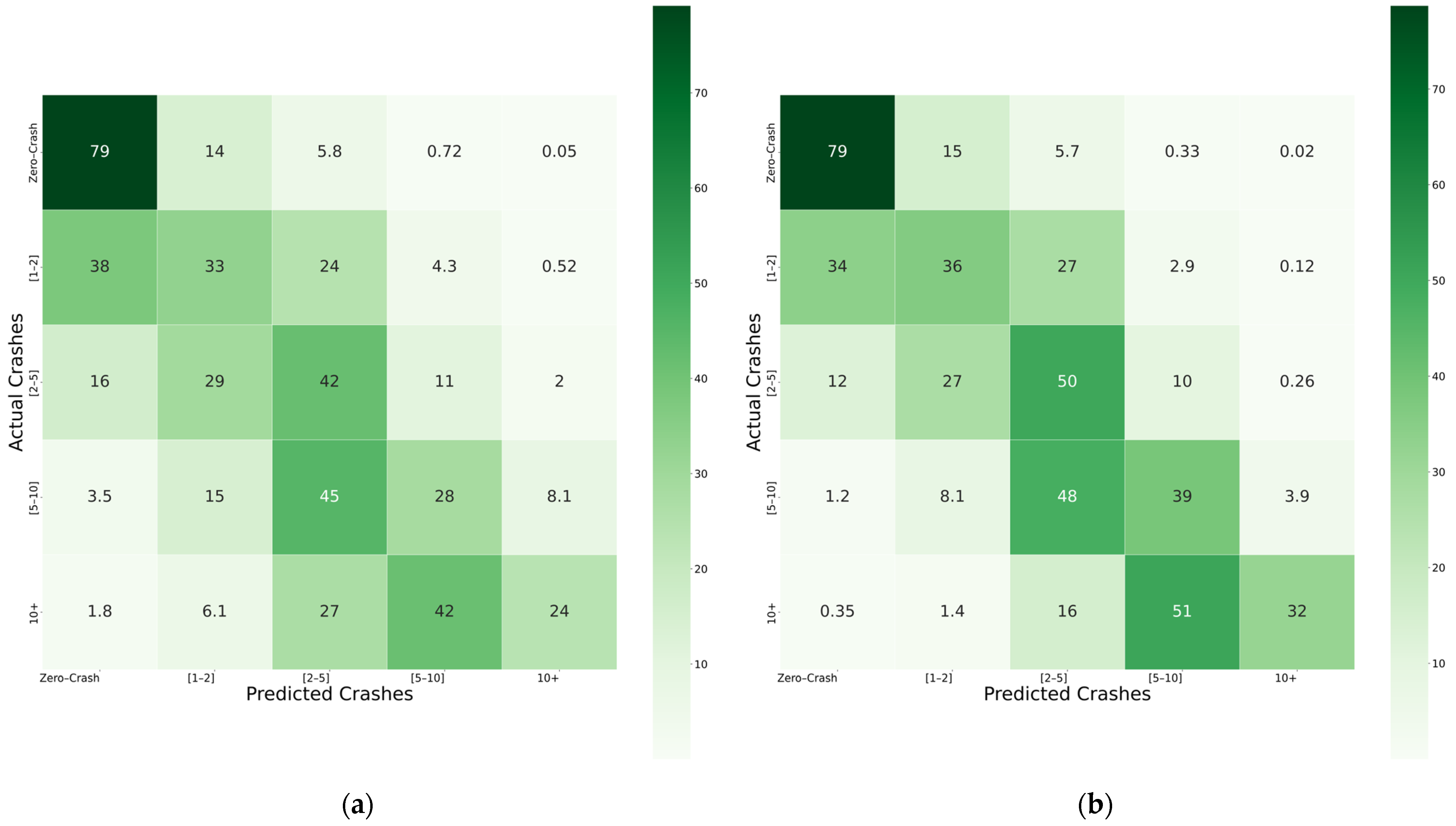
We further assessed the robustness of the RF model in predicting crash frequencies across different crash ranges using a confusion matrix. Figure 4a,b show the confusion matrices for both ZINB and RF models. The matrices provide a visual representation of the prediction accuracy for each range, with the diagonal line indicating the percentage of correct predictions. In predicting zero crashes, both models perform similarly, showing good accuracy in capturing segments with no crashes. However, for higher crash sites, the RF model depicts better accuracy with less deviation from the actual crash ranges. For example, in segments with fewer than 10 crashes, the RF model mistakenly predicts 1.2% as zero crashes, whereas ZINB predicts 3.5% as zero. Similarly, for segments with more than 10 crashes, the ZINB model incorrectly predicts 1.8% as zero crashes and 6.1% as 1–2 crashes, while the RF model makes fewer incorrect estimates, predicting only 0.35% as zero crashes and 1.4% as 1–2 crashes. These results indicate that the RF model offers a more accurate and reliable crash prediction across various crash ranges compared to the ZINB model. The ability of RF model to better identify segments with higher crash frequencies makes it a valuable tool for identifying high-risk locations and guiding the implementation of targeted safety improvement strategies.

5.4. Variable Importance & Interpretation of the Effect of Explanatory Variables

To measure how each explanatory variable affects RF model prediction, we employed the SHAP method introduced by Lundberg and Lee [71]. This technique allows us to explain tree-based machine learning models (including random forest) by quantifying the contribution of each variable to the model’s output for a specific instance, utilizing cooperative game theory [71,72]. Unlike other commonly used techniques such as LIME or LSA, SHAP captures both main and interaction effects among variables [73].
The SHAP method involves training two models to measure the contribution of a certain variable n. One model is trained with a subset of variables that includes the target variable n, while the other model is trained by excluding the target variable n from that subset. The marginal contribution of the variable n is then determined as the difference in the model prediction when including the variable and when excluding it. For any given prediction, the SHAP value for variable n is calculated as the weighted average of the marginal contributions across all possible subsets of variables. The general formula for calculating the SHAP value for variable n can be written as follows [71]:
ϕ n =   S F \ n S ! F S 1 ! F !   f S n x S n f S x S
where:
ϕ n = SHAP value for the explanatory variable n.
S = subset of explanatory variables.
F = set of all explanatory variables.
S = number of explanatory variables in subset S.
F = number of explanatory variables in set F.
f S n x S n = model prediction when adding the explanatory variable n to subset S.
f S x S = model prediction with explanatory variables in subset S.
SHAP estimates the contribution of each variable by assuming that model features are statistically independent. Under this assumption, SHAP replaces the conditional distribution of an explanatory variable with its marginal distribution when computing its effect [74]. When two variables are strongly correlated, this assumption can lead to uneven attribution: one correlated variable may receive a high SHAP value, while the other receives a much lower value because it does not add unique information beyond what the first variable already explains. To evaluate this concern in our dataset, we calculated the Variance Inflation Factor (VIF) for all inputs. All VIF values were below 3, indicating low multicollinearity and reducing the likelihood of unstable SHAP attributions [75].
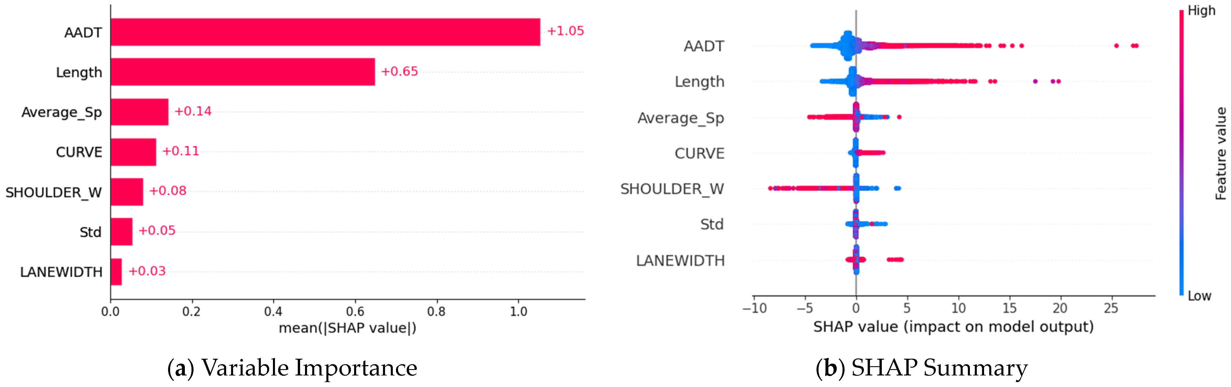
The estimated SHAP value was utilized as a measure of determining the most important factors for the model, and how they influence predictions. Figure 5a shows a global variable importance plot, where the global importance of each variable is calculated as the average of the absolute SHAP values across all instances in the dataset. The explanatory variables used in the RF model are ranked in descending order, starting from the top with the highest mean absolute SHAP value. Further, Figure 5b displays a SHAP summary plot, providing valuable insights into the impact of each explanatory variable on the predicted crashes. The plot depicts the explanatory variables on the vertical axis, arranged in descending order of importance. The horizontal axis shows the SHAP values. Variables with positive SHAP values indicate a positive influence on the model predictions, whereas negative SHAP values suggest a negative impact. The magnitude of the SHAP value denotes the strength of the impact. In addition, each point on the plot corresponds to the value of the respective explanatory variable. Red dots represent higher values of the explanatory variable, while lower values are represented by blue dots.
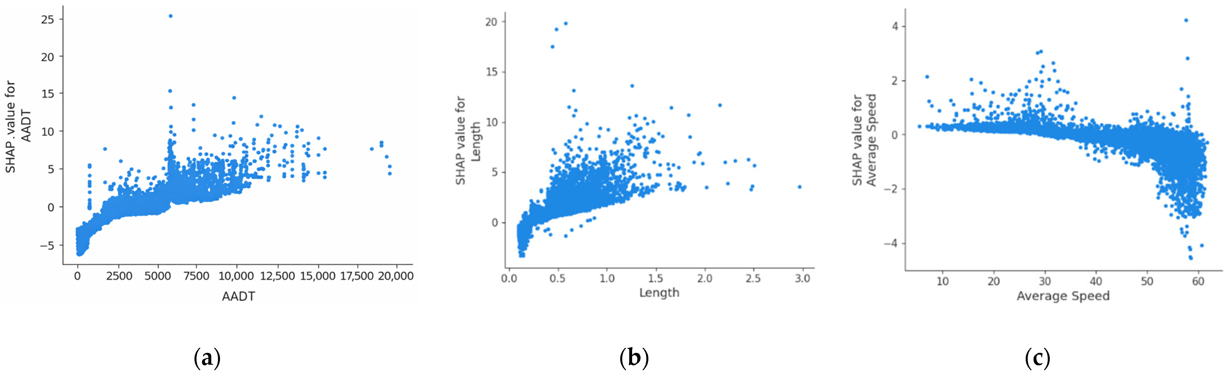
Upon analyzing Figure 5a,b, it is evident that AADT is the most influential variable (49.8%), followed by segment length (30.8%). These observations align with expectations, as both AADT and length are considered exposure variables, and their significance in crash prediction has been well established in previous studies [10,11,16,17]. Further examination of the variables showed that AADT and segment length have a positive effect on the number of crashes. This positive relationship is also confirmed by the SHAP dependence plots displayed in Figure 6a,b, where the SHAP values are plotted against AADT and segment length. These findings are consistent with previous studies that have identified higher traffic volumes and longer segments as contributing factors to increased crash occurrences [18,24,35].
Interestingly, the third-most important variable is average speed, contributing 6.7% to the model. This finding is particularly intriguing, as it showed up as more important than other geometric variables (e.g., shoulder width, curvature, and lane width) on two-lane highways. Furthermore, Figure 5b reveals that average speed has a negative influence on the crash frequencies, particularly in segments with high average speeds, while the opposite trend is observed in segments with low average speeds (also evident in Figure 6c). A more in-depth investigation of the dataset shows that higher speeds are typically observed on segments with better geometric conditions and vice versa. This observation can be further validated by assessing SHAP Interaction Plots, which are discussed later in this paper. Such observation supports data-driven prioritization of geometric improvements, particularly on segments with constrained speeds due to poor design features.
Among geometric variables, curvature and shoulder width are identified as the fourth- and fifth-most important variables, with contributions of 5.2% and 3.7%, respectively. Their effects align with expectations: sharp curvature tends to lead to more crashes, while wider shoulders tend to minimize them. These results provide useful guidance for low-cost safety countermeasures, such as shoulder widening, curve flattening, or delineation enhancements, which can yield substantial safety benefits on two-lane highways.
The std of speed and lane width have relatively negligible contributions (2.3% and 1.4%) to the model prediction. However, the minor but positive association between std of speed and crash frequency suggests that higher speed variability may reflect unstable traffic flow and higher crash potential. Such findings emphasize the need for design and management practices that promote uniform speeds along two-lane highways. This can be achieved by improving geometric alignment and speed management.
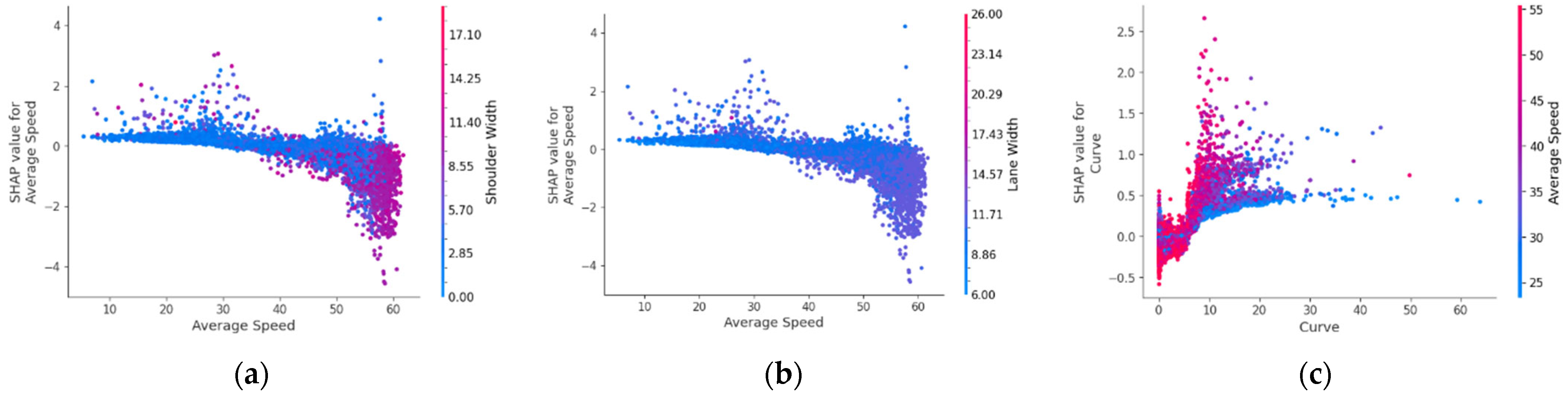
In this study, we also explored potential interactions between pairs of explanatory variables in relation to the model output using SHAP dependence plots. Figure 7 presents the identified interactions involving average speed, shoulder width, lane width, and curvature. The SHAP values are plotted against these variables, while the color of the points represents the value of the interacting variable. Figure 7a shows that as average speed increases, segments with wider shoulders (red points) tend to have lower crash frequencies, whereas, segments with narrow shoulders (blue points) exhibit higher crash frequencies. Figure 7b shows a similar pattern for lane width. Wider lanes (purple points) are associated with lower crash frequencies at higher speeds, while narrow lanes (blue points) correspond to increased crash frequencies. Figure 7c depicts the interaction between curvature and average speed. An increase in curvature tends to positively influence the predicted crashes. With smooth curves (curvature < 10 degrees), crashes are less frequent, even in segments with high average speeds (red points). However, the presence of sharp curves causes more crashes, even though the average speed is low.
Overall, the interaction plots in Figure 7 demonstrate that the average speed of two-lane highways reflects the geometric conditions and average traffic conditions. Segments operating at higher average speeds are generally characterized by wider lanes and shoulders and tend to have less crashes. Conversely, segments with lower average speeds are often associated with narrow shoulders and lanes, or with sharp curves, and are more prone to crashes. Therefore, average speed can be utilized as an indicator to capture the combined effects of roadway geometry and operating conditions. Incorporating this variable into safety assessments can help identify locations requiring geometric or operational improvements to enhance the safety performance of two-lane highways.

6. Application of the RF-SHAP-Informed Framework

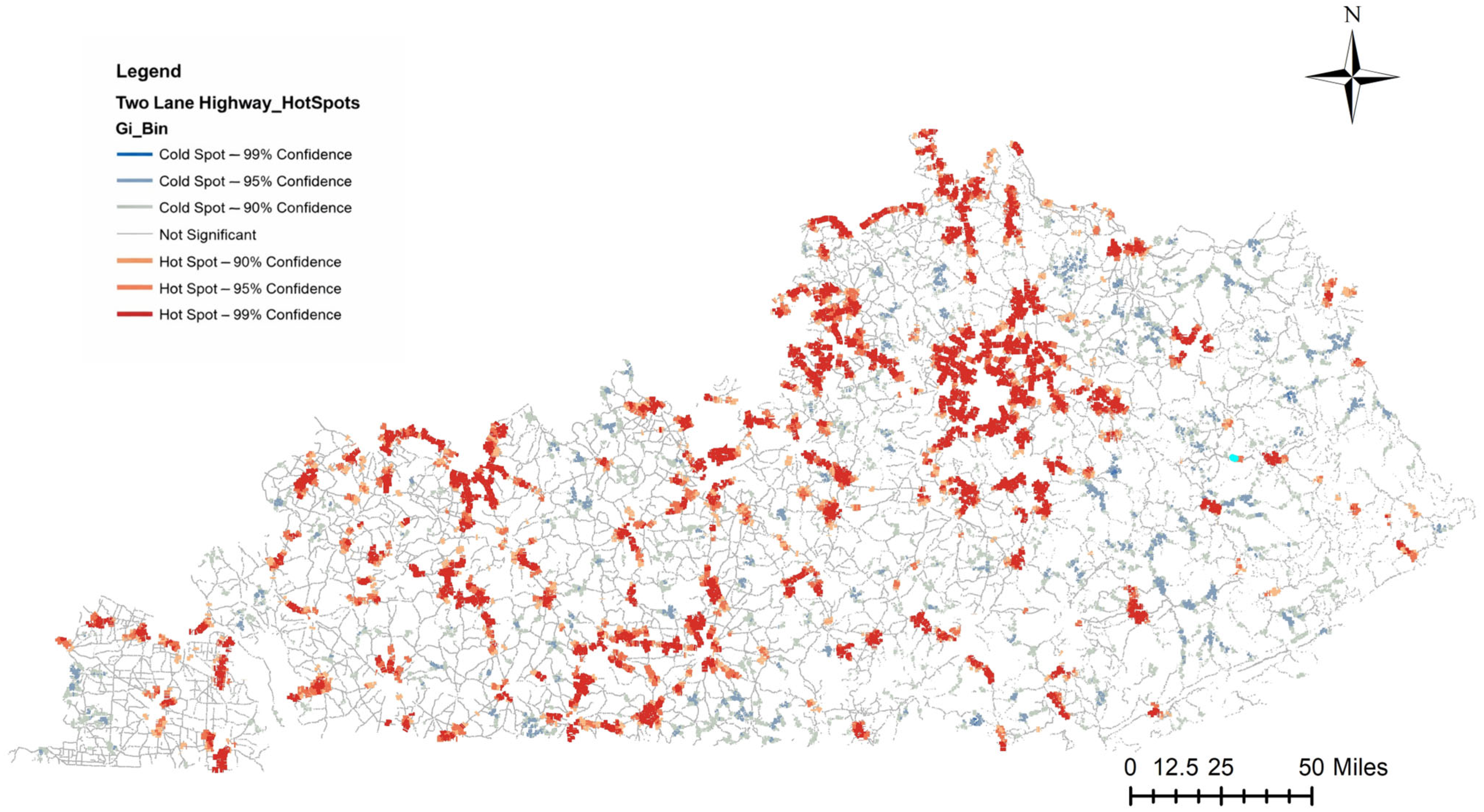
This study further demonstrates the application of the SHAP-based RF model framework in prioritizing segments for safety improvement and allocating resources. A hotspot analysis was first conducted using actual crash counts. A hotspot map (Figure 8) was developed to visualize the spatial distribution of high-crash segments across the study area.
From the complete set of hotspots showed in the map, a smaller group of segments was selected for the demonstration. Selection focused specifically on high-crash segments where at least one modifiable factor, such as curvature, average speed, std of speed, lane width, or shoulder width, appeared among the two highest-ranked variables (i.e., highest contributions in model predictions) from SHAP analysis for the individual segment. A step-by-step process for selecting countermeasures and prioritizing segments is discussed below.
  • Identification of Countermeasures based on SHAP Contributions:
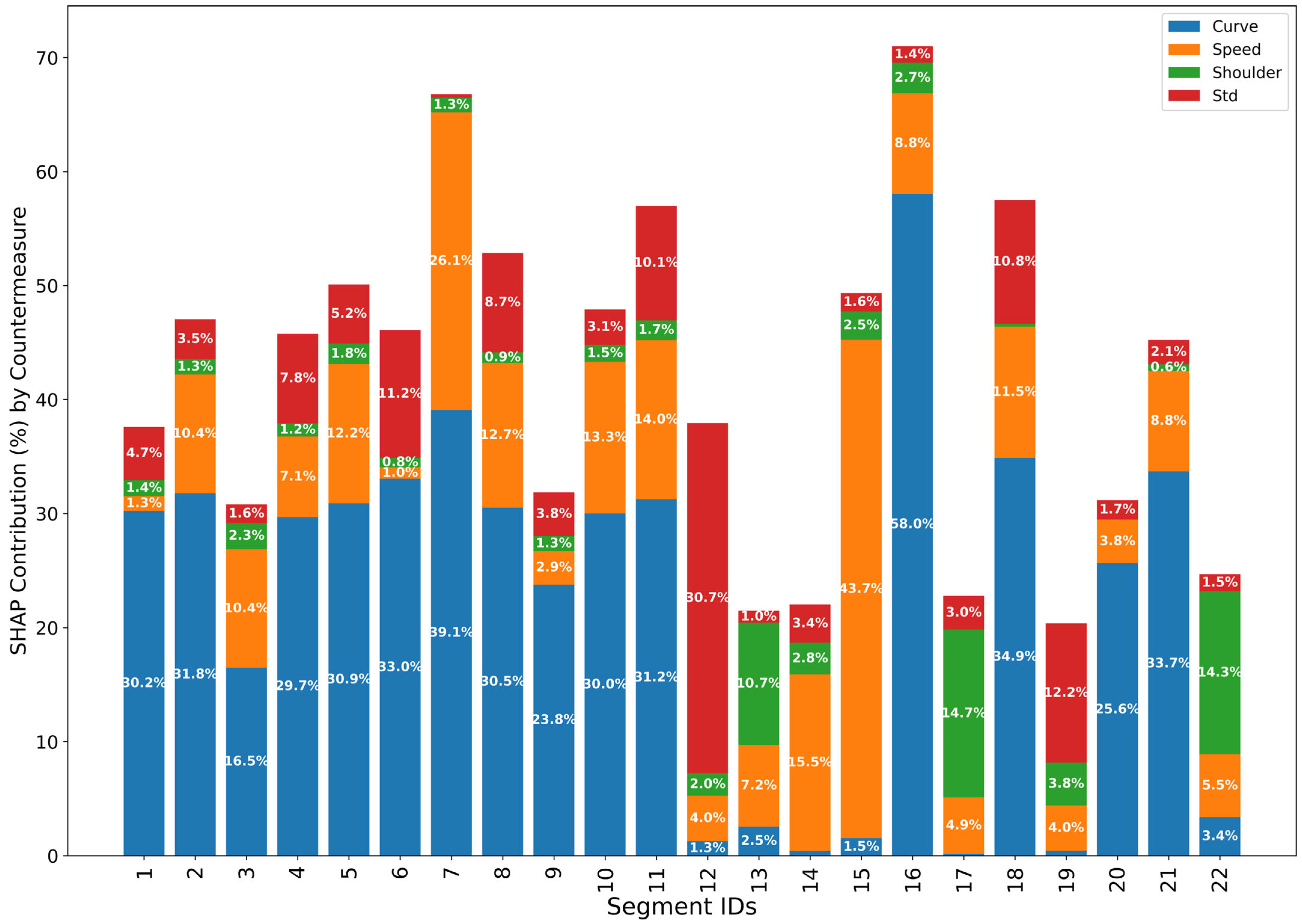
After evaluating SHAP contributions for individual factors in each segment, we selected four feasible countermeasures: curve flattening, speed limit adjustment, shoulder widening, and coordinated advisory speed. Figure 9 summarizes the percentage contribution of each countermeasure on the corresponding factors (curve, speed, shoulder, and std of speed) for all selected hotspots. Each bar represents one segment, with colored sections indicating the contribution of each countermeasure on the predicted crash. These contributions vary substantially across segments, showing that different modifiable crash factors dominate different locations. For each segment, the countermeasure with the highest SHAP contribution was designated as the priority treatment.
  • Expected Crash Reduction (ECR) After Applying Treatments and Segment Ranking:
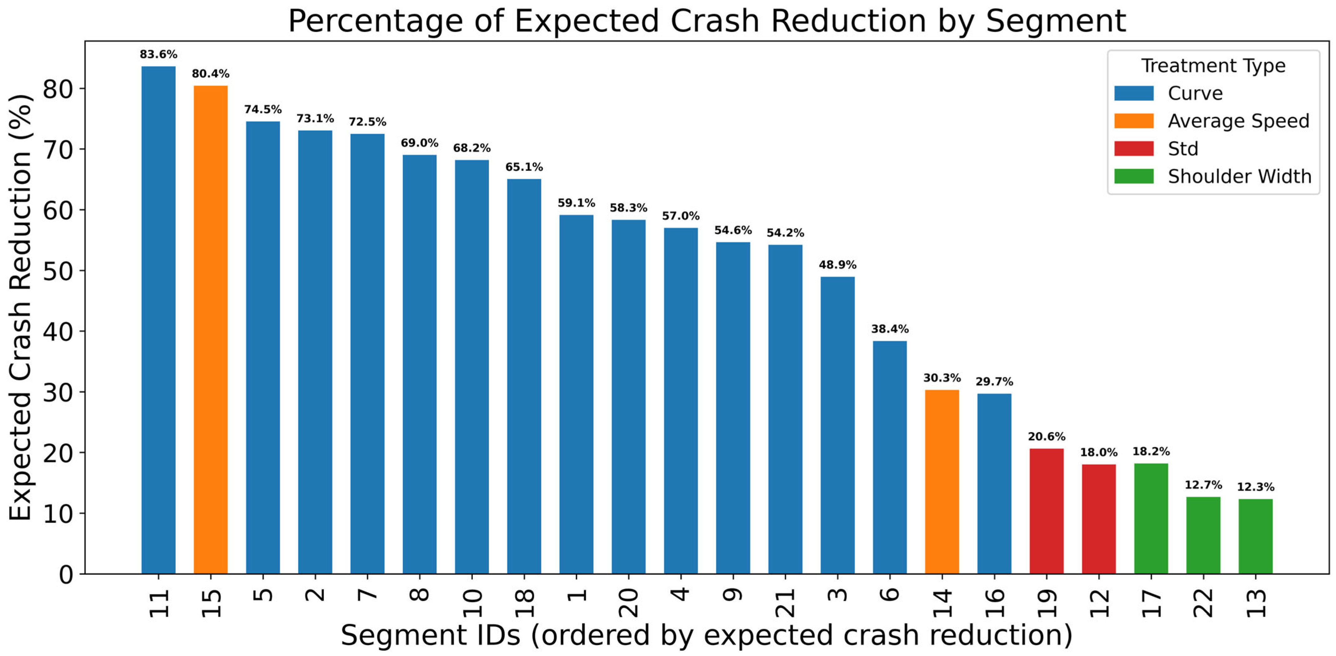
For each hotspot segment, the assigned priority treatment was applied by adjusting the relevant feature in the model inputs. Specifically, the treatment scenarios applied a 3° reduction in horizontal curvature, a 5 mph decrease in average speed, a 2 ft increase in shoulder width, and a 5 mph reduction in speed variability, depending on the priority treatment at that segment. The RF model then provided baseline and post-treatment crash predictions. The expected crash reduction (ECR) was calculated as the percentage decrease in predicted crashes compared to the baseline. Figure 10 displays ECR values in descending order. The results show substantial differences across segments, with some locations exhibiting reductions above 70%, while others show more moderate improvements. This ordering directly forms a priority list, where segments with the highest ECR appear first.
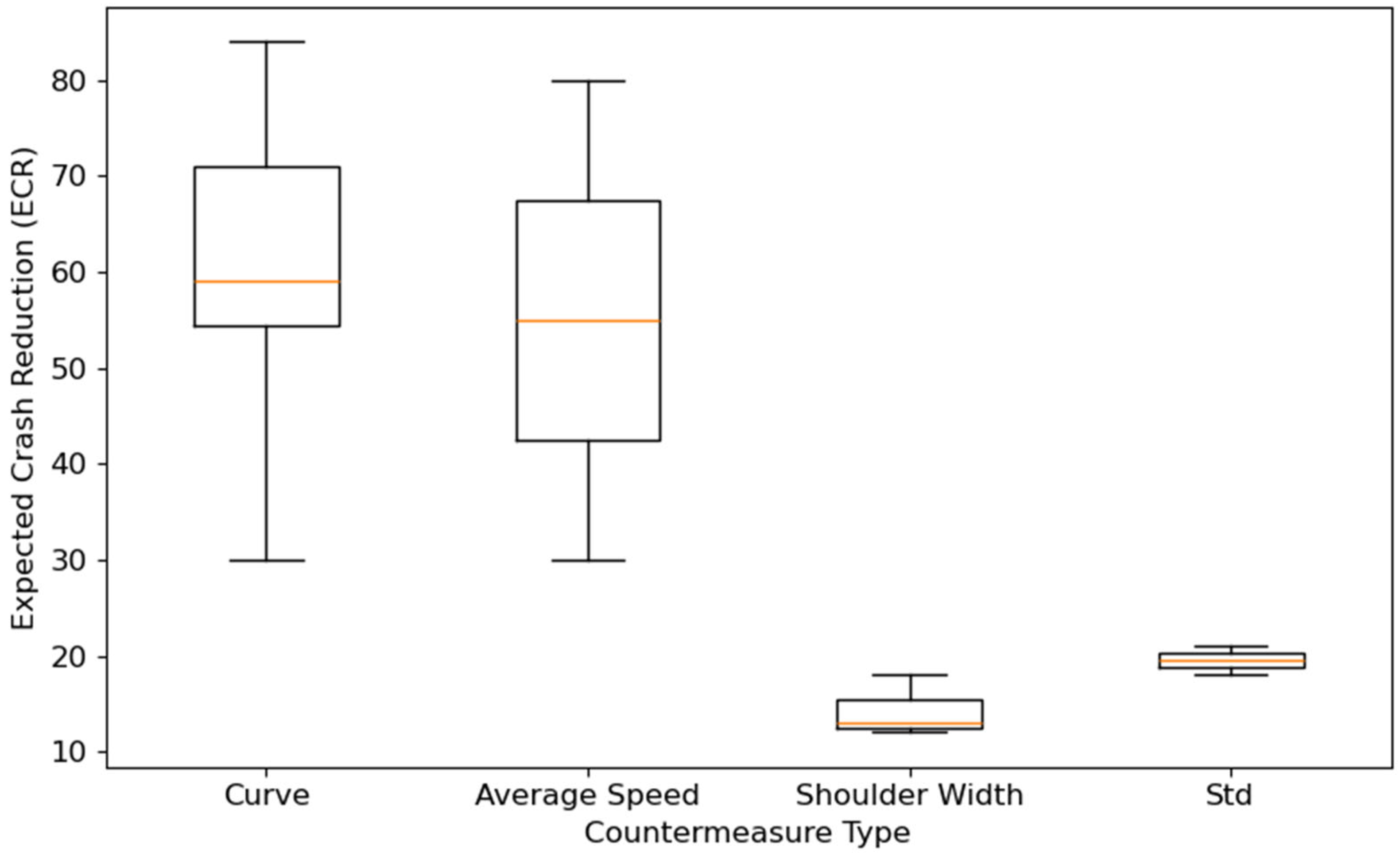
To assess the overall effectiveness of the countermeasures across the selected hotspots, the ECR values were grouped by priority treatment type and summarized in a boxplot (Figure 11). It compares the distributions of ECR for the previously mentioned treatments: curve, average speed, shoulder width, and speed variability. The boxplot reveals clear differences among treatment types. Curve and speed-related treatments show the highest median crash reductions, along with wider ranges, indicating that these treatments can yield substantial benefits at many locations but also vary by site-specific conditions. In contrast, shoulder-width treatments and speed variability treatments exhibit lower median reductions and narrower spreads, suggesting moderate but consistent improvements across sites.
  • Program-Level Resource Allocation
At the program level, the ECR estimates and the resulting segment rankings provide agencies with a practical basis for allocating resources. By comparing predicted safety benefits across locations, agencies can identify which projects offer the highest return on investment and prioritize those locations when budgets are limited. Ordering segments by ECR highlights where treatments are likely to produce the most significant improvements, enabling decision-makers to sequence projects strategically, plan multi-year safety programs, and balance cost, impact, and feasibility. This SHAP-informed ranking process offers a data-driven foundation for selecting projects that maximize overall safety gains with available resources.

7. Conclusions

This paper developed an integrated approach that combines an RF model with SHAP to link crash frequency on two-lane highways with traffic, geometric, and speed-related factors. The RF model was built using these variables and compared against the traditional statistical model, which is ZINB in this case. The comparison confirmed that the RF model significantly outperformed the ZINB model, with an improvement of up to 25% in terms of R2. Moreover, the CURE plots showed a good fit of the model as the cumulative residuals always remained within the accepted boundaries, whereas a substantial portion of the cumulative residuals were beyond the boundaries in the case of ZINB. Additionally, we investigated the RF model’s performance in identifying high-risk segments, and the results showed higher accuracy compared to the ZINB model. For example, when considering the segments with more than 10 crashes in Figure 4, the ZINB model incorrectly predicted 1.8% as zero crashes and 6.1% as 1–2 crashes, while the RF model made fewer incorrect estimates, predicting only 0.35% as zero crashes and 1.4% as 1–2 crashes. These results highlight the value of ML-based approaches for early-stage safety planning, where accurate prediction is essential for effective and sustainable decision-making.
This study further identified the most important factors affecting crash frequencies on two-lane highways and analyzed their contributions to RF model predictions using the SHAP method. As expected, AADT and length emerged as the top two variables, contributing 49.85% and 30.8%, respectively. Both variables showed a positive relationship with crash frequency, aligning with common expectations: higher traffic volume and longer road segments generally result in more crashes. Interestingly, average speed was found to be the third most important variable, with a 6.7% contribution. This highlights the critical role of speed beyond exposure-related measures in crash outcomes on two-lane highways. The finding also indicates that average speed played a more significant role in predicting crashes on these roads than geometric features such as shoulder width, curvature, and lane width.
Further investigation into the impact of average speed uncovered both negative and positive relationships with crash frequency on two-lane highways. The negative trend, in particular, can be attributed to the fact that two-lane highways with higher speeds are often the main corridors characterized by better geometric conditions [63,76]. This can be further confirmed by investigating the complex interactions between different roadway attributes and their effects on crash predictions. The analysis of the interactions in Figure 7a,b showed that crashes tend to occur less on the segments with higher average speeds, and these segments have wider shoulders and lanes. This suggests that the average speed of two-lane highways somehow reflects the overall geometric conditions and average traffic conditions on these roads. In cases where combining geometric and traffic conditions can be challenging, average speed can be a valuable measure that effectively captures the effect of these factors.
Overall, the RF model outperformed the traditional model, offering enhanced flexibility to incorporate a larger set of explanatory variables. It effectively captured complex non-linear relationships and interactions among variables. The integration of the SHAP method further enhanced the model’s interpretability by providing valuable insights into variable importance, the direction and magnitude of their effects on crashes, and the influence of variable interactions on the model predictions. Importantly, the primary contribution of this study lies in the framework, rather than in the specific variable rankings observed in Kentucky. The proposed RF–SHAP framework is transferable and can be adapted by other agencies using their own data to identify locally relevant risk factors, including speed-related measures. This study further demonstrates how this framework can support project prioritization and resource allocation by linking interpretable model outputs to expected crash reduction estimates. By identifying modifiable risk factors, estimating safety benefits of feasible countermeasures, and ranking segments based on predicted impact, the framework provides a clear decision support pathway for safety investment planning.
From a sustainability perspective, the proposed approach supports resource-efficient road safety management by helping agencies target interventions where the greatest safety gains can be achieved with limited resources. By explicitly incorporating speed into crash prediction and prioritization, the framework aligns safety improvement efforts with broader sustainability goals, including reduced crash-related societal costs, more efficient use of public funds, and long-term improvements in roadway safety performance. As such, the RF–SHAP framework offers a practical, data-informed tool for advancing sustainable safety management on two-lane highway networks.

8. Limitations and Future Work

Although the Random Forest model performed well in predicting crashes on Kentucky’s two-lane highways, several limitations should be acknowledged. The current analysis was limited to one state. In addition, the variables primarily represented roadway geometry, traffic control, and speed-related measures; other influencing factors, such as weather conditions, surface conditions, and real-time traffic data, were not included due to limited data availability. This study also concentrated solely on crash frequency, leaving the crash severity aspect unexplored.
Future studies will continue to validate the developed model using crash data from other regions to evaluate its generalizability and applicability beyond Kentucky’s two-lane highways. Such cross-regional validation would help confirm the transferability of the developed model and strengthen its potential for broader implementation. Expanding the input variables to include environmental and temporal factors could improve model performance and offer a more complete understanding of crash occurrence.
Future research will also explore the robustness of the RF model in predicting crashes across varying severity levels. Such analysis could provide valuable insights into the factors contributing to varying levels of crash severity and help tailor safety interventions accordingly. Furthermore, exploring advanced modeling techniques, such as deep learning methods, may provide additional accuracy and capture more complex patterns in crashes.

Author Contributions

Conceptualization, F.R. and X.Z.; methodology, F.R., X.Z., C.S. and M.C.; formal analysis, F.R., X.Z., C.S. and M.C.; investigation, F.R., X.Z., C.S. and M.C.; data curation, F.R. and X.Z.; writing—original draft preparation, F.R., X.Z., C.S. and M.C.; writing—review and editing, F.R., X.Z., C.S. and M.C.; supervision, M.C. All authors have read and agreed to the published version of the manuscript.

Funding

This research received no external funding.

Institutional Review Board Statement

Not applicable.

Informed Consent Statement

Not applicable.

Data Availability Statement

The crash data used in this study are available at Kentucky State Police (http://crashinformationky.org/AdvancedSearch, accessed on 1 January 2019). Road attributes are available at Highway Information System (https://transportation.ky.gov/Planning/Pages/Centerlines.aspx, accessed on 1 January 2019). Lastly, HERE speed data is proprietary and would not be made available due to the restriction of the data use agreement.

Acknowledgments

The authors would like to thank Eric Green and William Staats for their assistance in crash data management and pre-processing works. In addition, the authors would like to acknowledge ChatGPT 5 since it was used to improve readability and language while preparing the manuscript.

Conflicts of Interest

The authors declare no conflict of interest.

Abbreviations

The following abbreviations are used in this manuscript:
AADTAnnual Average Daily Traffic
SPFSafety Performance Function
CMFcrash modification factors
AASHTOAmerican Association of State Highway and Transportation Officials
HSMHighway Safety Manual
SHAPSHapley Additive exPlanations
ZINBZero-inflated Negative Binomial
HISHighway Information System
CV Cross-Validation
PCCPearson Correlation Coefficient
MSEMean Squared Error
MADMean Absolute Deviation

References

  1. Lovegrove, G.R.; Sayed, T. Using Macrolevel Collision Prediction Models in Road Safety Planning Applications. Transp. Res. Rec. 2006, 1950, 73–82. [Google Scholar]
  2. Lovegrove, G.R.; Sayed, T. Macrolevel Collision Prediction Models to Enhance Traditional Reactive Road Safety Improvement Programs. Transp. Res. Rec. 2007, 2019, 65–73. [Google Scholar]
  3. HSM. Highway Safety Manual Part C, 1st ed.; AASHTO: Washington, DC, USA, 2010; Volume 2. [Google Scholar]
  4. ODOT. Analysis Procedures Manual. 1205; Oregon Department of Transportation: Salem, ON, USA, 2025. [Google Scholar]
  5. Rajabi, M.; Ogle, J.H.; Gerard, P. Highway Safety Manual Calibration: Assessing Alternate Definitions of the Calibration Factor. Transp. Res. Rec. 2018, 2672, 99–108. [Google Scholar]
  6. Ijaz, M.; Lan, L.; Zahid, M.; Jamal, A. A Comparative Study of Machine Learning Classifiers for Injury Severity Prediction of Crashes Involving Three-Wheeled Motorized Rickshaw. Accid. Anal. Prev. 2021, 154, 106094. [Google Scholar] [CrossRef]
  7. Iranitalab, A.; Khattak, A. Comparison of Four Statistical and Machine Learning Methods for Crash Severity Prediction. Accid. Anal. Prev. 2017, 108, 27–36. [Google Scholar] [CrossRef]
  8. Lord, D.; Mannering, F. The Statistical Analysis of Crash-Frequency Data: A Review and Assessment of Methodological Alternatives. Transp. Res. Part A Policy Pract. 2010, 44, 291–305. [Google Scholar]
  9. Pan, G.; Fu, L.; Thakali, L. Development of a Global Road Safety Performance Function Using Deep Neural Networks. Int. J. Transp. Sci. Technol. 2017, 6, 159–173. [Google Scholar] [CrossRef]
  10. Pu, Z.; Li, Z.; Ke, R.; Hua, X.; Wang, Y. Evaluating the Nonlinear Correlation between Vertical Curve Features and Crash Frequency on Highways Using Random Forests. J. Transp. Eng. Part A Syst. 2020, 146, 04020115. [Google Scholar]
  11. Wen, X.; Xie, Y.; Jiang, L.; Li, Y.; Ge, T. On the Interpretability of Machine Learning Methods in Crash Frequency Modeling and Crash Modification Factor Development. Accid. Anal. Prev. 2022, 168, 106617. [Google Scholar] [CrossRef]
  12. Zeng, Q.; Huang, H.; Pei, X.; Wong, S.; Gao, M. Rule Extraction from an Optimized Neural Network for Traffic Crash Frequency Modeling. Accid. Anal. Prev. 2016, 97, 87–95. [Google Scholar] [CrossRef]
  13. Das, S.; Sun, X.; Sun, M. Rule-Based Safety Prediction Models for Rural Two-Lane Run-Off-Road Crashes. Int. J. Transp. Sci. Technol. 2021, 10, 235–244. [Google Scholar] [CrossRef]
  14. Yu, R.; Abdel-Aty, M. Utilizing Support Vector Machine in Real-Time Crash Risk Evaluation. Accid. Anal. Prev. 2013, 51, 252–259. [Google Scholar] [CrossRef] [PubMed]
  15. Tayebikhorami, S.; Sacchi, E. Validation of Machine Learning Algorithms as Predictive Tool in the Road Safety Management Process: Case of Network Screening. J. Transp. Eng. Part A Syst. 2022, 148, 04022068. [Google Scholar]
  16. Saha, D.; Alluri, P.; Gan, A. Prioritizing Highway Safety Manual’s Crash Prediction Variables Using Boosted Regression Trees. Accid. Anal. Prev. 2015, 79, 133–144. [Google Scholar] [CrossRef]
  17. Wei, Z.; Das, S.; Zhang, Y. Short Duration Crash Prediction for Rural Two-Lane Roadways: Applying Explainable Artificial Intelligence. Transp. Res. Rec. 2022, 2676, 535–549. [Google Scholar]
  18. Anderson, I.B.; Bauer, K.M.; Harwood, D.W.; Fitzpatrick, K. Relationship to Safety of Geometric Design Consistency Measures for Rural Two-Lane Highways. Transp. Res. Rec. 1999, 1658, 43–51. [Google Scholar] [CrossRef]
  19. Bornheimer, C. Finding a New Safety Performance Function for Two-Way, Two-Lane Highways in Rural Areas. Doctoral Dissertation, University of Kansas, Lawrence, KS, USA, 2011. [Google Scholar]
  20. Cafiso, S.; Di Graziano, A.; Di Silvestro, G.; La Cava, G.; Persaud, B. Development of Comprehensive Accident Models for Two-Lane Rural Highways Using Exposure, Geometry, Consistency and Context Variables. Accid. Anal. Prev. 2010, 42, 1072–1079. [Google Scholar] [CrossRef]
  21. De Oña, J.; Garach, L. Accidents Prediction Model Based on Speed Reduction on Spanish Two-Lane Rural Highways. Procedia-Soc. Behav. Sci. 2012, 53, 1010–1018. [Google Scholar]
  22. Huang, H.; Chin, H.C. Modeling Road Traffic Crashes with Zero-Inflation and Site-Specific Random Effects. Stat. Methods Appl. 2010, 19, 445–462. [Google Scholar]
  23. Kweon, Y.J.; Kockelman, K.M. Safety Effects of Speed Limit Changes: Use of Panel Models, Including Speed, Use, and Design Variables. Transp. Res. Rec. 2005, 1908, 148–158. [Google Scholar] [CrossRef]
  24. Llopis-Castelló, D.; Bella, F.; Camacho-Torregrosa, F.J.; García, A. New Consistency Model Based on Inertial Operating Speed Profiles for Road Safety Evaluation. J. Transp. Eng. Part A Syst. 2018, 144, 10. [Google Scholar]
  25. Dutta, N.; Fontaine, M.D. Developing Rural Four Lane Freeway Crash Prediction Models Using Hourly Flow Parameters. In Proceedings of the TRB 2019 Annual Meeting, Washington, DC, USA, 13–17 January 2019. [Google Scholar]
  26. Sharma, A.K.; Landge, V.S. Zero Inflated Negative Binomial for Modeling Heavy Vehicle Crash Rate on Indian Rural Highway. Int. J. Adv. Eng. Technol. 2013, 5, 292. [Google Scholar]
  27. Wang, C.; Quddus, M.; Ison, S. The Effects of Area-Wide Road Speed and Curvature on Traffic Casualties in England. J. Transp. Geogr. 2009, 17, 385–395. [Google Scholar] [CrossRef]
  28. Xu, J.; Kockelman, K.M.; Wang, Y. Modeling Crash and Fatality Counts Along Mainlanes and Frontage Roads across Texas: The Roles of Design, the Built Environment, and Weather. In Proceedings of the 93rd Annual Meeting of the Transportation Research, Washington, DC, USA, 12–16 January 2014. [Google Scholar]
  29. Yan, X.; Wang, B.; An, M.; Zhang, C. Distinguishing between Rural and Urban Road Segment Traffic Safety Based on Zero-Inflated Negative Binomial Regression Models. Discret. Dyn. Nat. Soc. 2012, 2012, 11. [Google Scholar] [CrossRef]
  30. Kockelman, K.K.; Ma, J. Freeway Speeds and Speed Variations Preceding Crashes, within and across Lanes. J. Transp. Res. Forum 2007, 46, 1. [Google Scholar]
  31. Lave, C.A. Speeding, Coordination, and the 55 Mph Limit. Am. Econ. Rev. 1985, 75, 1159–1164. [Google Scholar]
  32. Ma, J.; Kockelman, K.M.; Damien, P. A Multivariate Poisson-Lognormal Regression Model for Prediction of Crash Counts by Severity, Using Bayesian Methods. Accid. Anal. Prev. 2008, 40, 964–975. [Google Scholar] [CrossRef]
  33. Stapleton, S.Y.; Ingle, A.J.; Chakraborty, M.; Gates, T.J.; Savolainen, P.T. Safety Performance Functions for Rural Two-Lane County Road Segments. Transp. Res. Rec. 2018, 2672, 226–237. [Google Scholar]
  34. Wang, K.; Ivan, J.N.; Ravishanker, N.; Jackson, E. Multivariate Poisson Lognormal Modeling of Crashes by Type and Severity on Rural Two Lane Highways. Accid. Anal. Prev. 2017, 99, 6–19. [Google Scholar] [CrossRef]
  35. Wu, K.-F.; Donnell, E.T.; Himes, S.C.; Sasidharan, L. Exploring the Association between Traffic Safety and Geometric Design Consistency Based on Vehicle Speed Metrics. J. Transp. Eng. Part A Syst. 2013, 139, 738–748. [Google Scholar]
  36. Hezaveh, A.M.; Arvin, R.; Cherry, C.R. A Geographically Weighted Regression to Estimate the Comprehensive Cost of Traffic Crashes at a Zonal Level. Accid. Anal. Prev. 2019, 131, 15–24. [Google Scholar] [CrossRef]
  37. Li, Z.; Wang, W.; Liu, P.; Bigham, J.M.; Ragland, D.R. Using Geographically Weighted Poisson Regression for County-Level Crash Modeling in California. Saf. Sci. 2013, 58, 89–97. [Google Scholar] [CrossRef]
  38. Liu, J.; Khattak, A.J.; Wali, B. Do Safety Performance Functions Used for Predicting Crash Frequency Vary across Space? Applying Geographically Weighted Regressions to Account for Spatial Heterogeneity. Accid. Anal. Prev. 2017, 109, 132–142. [Google Scholar] [CrossRef] [PubMed]
  39. Mathew, S.; Pulugurtha, S.S.; Duvvuri, S. Exploring the Effect of Road Network, Demographic, and Land Use Characteristics on Teen Crash Frequency Using Geographically Weighted Negative Binomial Regression. Accid. Anal. Prev. 2022, 168, 106615. [Google Scholar] [CrossRef] [PubMed]
  40. Mohammadnazar, A.; Mahdinia, I.; Ahmad, N.; Khattak, A.J.; Liu, J. Understanding How Relationships between Crash Frequency and Correlates Vary for Multilane Rural Highways: Estimating Geographically and Temporally Weighted Regression Models. Accid. Anal. Prev. 2021, 157, 106146. [Google Scholar] [CrossRef] [PubMed]
  41. Wang, C.; Li, S.; Shan, J. Non-Stationary Modeling of Microlevel Road-Curve Crash Frequency with Geographically Weighted Regression. ISPRS Int. J. Geo-Inf. 2021, 10, 286. [Google Scholar] [CrossRef]
  42. Nelder, J.A.; Wedderburn, R.W. Generalized Linear Models. J. R. Stat. Soc. Ser. A Stat. Soc. 1972, 135, 370–384. [Google Scholar]
  43. Li, X.; Lord, D.; Zhang, Y.; Xie, Y. Predicting Motor Vehicle Crashes Using Support Vector Machine Models. Accid. Anal. Prev. 2008, 40, 1611–1618. [Google Scholar] [CrossRef]
  44. Zhang, Z.; Nie, Q.; Liu, J.; Hainen, A.; Islam, N.; Yang, C. Machine Learning Based Real-Time Prediction of Freeway Crash Risk Using Crowdsourced Probe Vehicle Data. J. Intell. Transp. Syst. 2024, 28, 84–102. [Google Scholar]
  45. Yu, R.; Abdel-Aty, M. Analyzing Crash Injury Severity for a Mountainous Freeway Incorporating Real-Time Traffic and Weather Data. Saf. Sci. 2014, 63, 50–56. [Google Scholar] [CrossRef]
  46. Sakib, N.; Paul, T.; Das, S.; Hossain, A. Exploring the Factors Affecting Injury Severity in Highway and Non-Highway Crashes in Bangladesh Applying Machine Learning and Shap. IATSS Res. 2025, 49, 259–270. [Google Scholar] [CrossRef]
  47. Owais, M.; Alshehri, A.; Gyani, J.; Aljarbou, M.H.; Alsulamy, S. Prioritizing Rear-End Crash Explanatory Factors for Injury Severity Level Using Deep Learning and Global Sensitivity Analysis. Expert Syst. Appl. 2024, 245, 123114. [Google Scholar] [CrossRef]
  48. Moussa, G.S.; Owais, M.; Dabbour, E. Variance-Based Global Sensitivity Analysis for Rear-End Crash Investigation Using Deep Learning. Accid. Anal. Prev. 2022, 165, 106514. [Google Scholar] [PubMed]
  49. Green, E.R. Segmentation Strategies for Road Safety Analysis. Doctoral Dissertation, Doctor of Philosophy, University of Kentucky, Lexington, KY, USA, 2018. [Google Scholar]
  50. Green, E.R.; Blackden, C.; Fields, M.A. Spatial Database for Intersections; University of Kentucky Transportation Center: Lexington, KY, USA, 2015. [Google Scholar]
  51. Hauer, E.; Bamfo, J. Two Tools for Finding What Function Links the Dependent Variable to the Explanatory Variables. In Proceedings of the ICTCT 1997 Conference, Lund, Sweden, 5–7 November 1997. [Google Scholar]
  52. Available online: https://www.here.com/ (accessed on 1 January 2018).
  53. Zhang, X.; Chen, M. Methodology for Conflating Large-Scale Roadway Networks. Transp. Res. Rec. J. Transp. Res. Board 2022, 2677, 189–202. [Google Scholar] [CrossRef]
  54. Li, S.; Zhu, K.; van Gelder, B.H.W.; Nagle, J.; Tuttle, C. Reconsideration of Sample Size Requirements for Field Traffic Data Collection with Global Positioning System Devices. Transp. Res. Rec. 2002, 1804, 17–22. [Google Scholar]
  55. Crunkleton, J.L.; Tarnoff, P.J. Statistical Patterns of Traffic Data and Sample Size Estimation; Center for Advanced Transportation Technology: College Park, MD, USA, 2015. [Google Scholar]
  56. Breiman, L. Random Forests. Mach. Learn. 2001, 45, 5–32. [Google Scholar]
  57. Gong, H.; Sun, Y.; Shu, X.; Huang, B. Use of Random Forests Regression for Predicting Iri of Asphalt Pavements. Constr. Build. Mater. 2018, 189, 890–897. [Google Scholar] [CrossRef]
  58. Svetnik, V.; Liaw, A.; Tong, C.; Culberson, J.C.; Sheridan, R.P.; Feuston, B.P. Random Forest: A Classification and Regression Tool for Compound Classification and Qsar Modeling. J. Chem. Inf. Comput. Sci. 2003, 43, 1947–1958. [Google Scholar] [CrossRef]
  59. Li, P.; Abdel-Aty, M.; Yuan, J. Real-Time Crash Risk Prediction on Arterials Based on Lstm-Cnn. Accid. Anal. Prev. 2020, 135, 105371. [Google Scholar] [CrossRef]
  60. Han, S.; Williamson, B.D.; Fong, Y. Improving Random Forest Predictions in Small Datasets from Two-Phase Sampling Designs. BMC Med. Inform. Decis. Mak. 2021, 21, 322. [Google Scholar]
  61. Parmar, H.; Bhanderi, S.; Shah, G. Sentiment Mining of Movie Reviews Using Random Forest with Tuned Hyperparameters. In Proceedings of the International Conference on Information Science, Kerala, India, 4–5 July 2014. [Google Scholar]
  62. Probst, P.; Wright, M.N.; Boulesteix, A. Hyperparameters and Tuning Strategies for Random Forest. Wiley Interdiscip. Rev. Data Min. Knowl. Discov. 2019, 9, e1301. [Google Scholar] [CrossRef]
  63. Rahman, F.; Zhang, X.; Chen, M. Evaluating Effect of Operating Speed on Crashes of Rural Two-Lane Highways. J. Adv. Transp. 2023, 2023, 2882951. [Google Scholar] [CrossRef]
  64. Saha, D.; Alluri, P.; Gan, A. A Random Forests Approach to Prioritize Highway Safety Manual (Hsm) Variables for Data Collection. J. Adv. Transp. 2016, 50, 522–540. [Google Scholar]
  65. Genuer, R.; Poggi, J.M.; Tuleau-Malot, C. Variable Selection Using Random Forests. Pattern Recognit. Lett. 2010, 31, 2225. [Google Scholar] [CrossRef]
  66. Lord, D.; Washington, S.; Ivan, J.N. Further Notes on the Application of Zero-Inflated Models in Highway Safety. Accid. Anal. Prev. 2007, 39, 53–57. [Google Scholar] [CrossRef] [PubMed]
  67. Lord, D.; Washington, S.P.; Ivan, J.N. Poisson, Poisson-Gamma and Zero-Inflated Regression Models of Motor Vehicle Crashes: Balancing Statistical Fit and Theory. Accid. Anal. Prev. 2005, 37, 35–46. [Google Scholar] [PubMed]
  68. Raihan, A.; Alluri, P.; Wu, W.; Gan, A. Estimation of Bicycle Crash Modification Factors (Cmfs) on Urban Facilities Using Zero Inflated Negative Binomial Models. Accid. Anal. Prev. 2019, 123, 303–313. [Google Scholar] [CrossRef] [PubMed]
  69. Lee, J.; Abdel-Aty, M.; Shah, I. Evaluation of Surrogate Measures for Pedestrian Trips at Intersections and Crash Modeling. Accid. Anal. Prev. 2019, 130, 91–98. [Google Scholar] [CrossRef]
  70. Rahman, F. Incorporating Speed into Crash Modeling for Rural Two-Lane Highways. 2022. Available online: https://uknowledge.uky.edu/ce_etds/121/ (accessed on 1 July 2023).
  71. Lundberg, S.M.; Lee, S.I. A Unified Approach to Interpreting Model Predictions. Adv. Neural Inf. Process. Syst. 2017, 30, 1–10. [Google Scholar]
  72. Lee, J.; Mannering, F. Impact of Roadside Features on the Frequency and Severity of Run-Off-Roadway Accidents: An Empirical Analysis. Accid. Anal. Prev. 2002, 34, 149–161. [Google Scholar]
  73. Ali, Y.; Hussain, F.; Haque, M. Advances, Challenges, and Future Research Needs in Machine Learning-Based Crash Prediction Models: A Systematic Review. Accid. Anal. Prev. 2024, 194, 107378. [Google Scholar] [CrossRef]
  74. Salih, A.M. Explainable Artificial Intelligence for Dependent Features: Additive Effects of Collinearity. In Proceedings of the 2024 8th International Conference on Advances in Artificial Intelligence, London, UK, 17–19 October 2024. [Google Scholar]
  75. Shrestha, N. Detecting Multicollinearity in Regression Analysis. Am. J. Appl. Math. Stat. 2020, 8, 39–42. [Google Scholar] [CrossRef]
  76. Pei, X.; Wong, S.; Sze, N. The Roles of Exposure and Speed in Road Safety Analysis. Accid. Anal. Prev. 2012, 48, 464–471. [Google Scholar] [CrossRef]
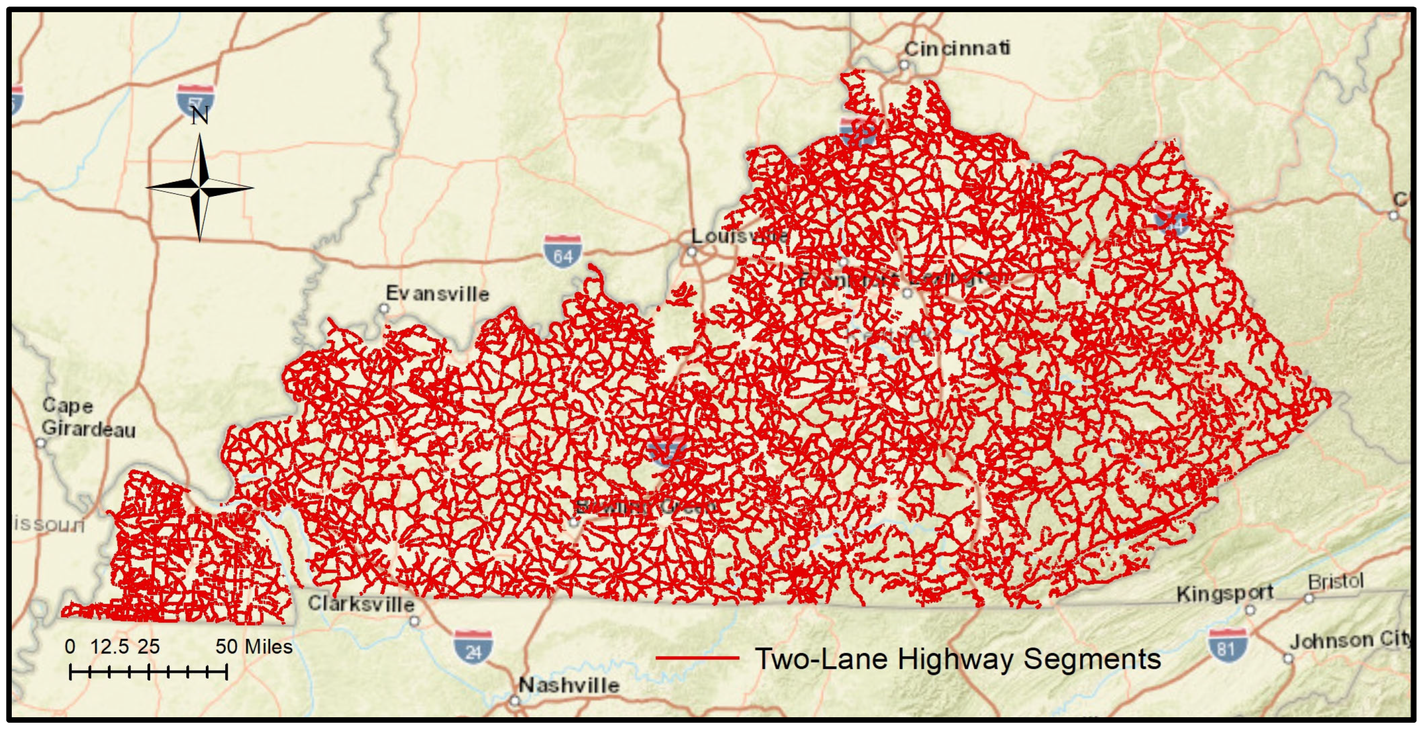
Figure 1. Two-Lane Highway Segments in Kentucky.
Sustainability 18 00635 g001
Figure 2. Overall Process of Applying the RF Model in Identifying Factors of Two-Lane Highways Crashes.
Sustainability 18 00635 g002
Figure 3. Comparison of CURE Plots: (a) ZINB Model and (b) RF Model.
Sustainability 18 00635 g003
Figure 4. Comparison of ZINB and RF Model Performance with Confusion Matrix: (a) ZINB Model and (b) RF Model.
Sustainability 18 00635 g004
Figure 5. Variable Importance Plot & SHAP Summary Plot.
Sustainability 18 00635 g005
Figure 6. SHAP Dependence Plots for (a) AADT, (b) Length, and (c) Average Speed.
Sustainability 18 00635 g006
Figure 7. SHAP Interaction Plots. Interactions between (a) Average Speed and Shoulder Width, (b) Average Speed and Lane Width, and (c) Curvature and Average Speed.
Sustainability 18 00635 g007
Figure 8. Spatial Distribution of the High Crash Segments.
Sustainability 18 00635 g008
Figure 9. SHAP Contributions for Selected Countermeasures.
Sustainability 18 00635 g009
Figure 10. Percentage of Expected Crash Reduction by Segment.
Sustainability 18 00635 g010
Figure 11. Distribution of Expected Crash Reduction by Treatment Type.
Sustainability 18 00635 g011
Table 1. Summary Statistics of Roadway Characteristics.
VariablesUnitStatistics
Min.The 25th PercentileMedianThe 75th PercentileMax.
AADTvehicles2310675161719,619
Segment Length (l)km0.20.20.30.54.7
Curvature (cu)degrees0.00.20.83.663.8
Lane Width (lw)m1.82.72.73.05.5
Shoulder Width (sw)m0.00.60.91.24.3
Average Speed (va)kmph8.752.864.676.599.5
Standard Deviation (std) of Speedkmph10.021.125.731.159.1
The 85th Percentile Speed (v85)kmph20.869.579.188.7108.3
Crash Frequencies in 5 years 0001161
Table 2. Optimization of Hyperparameters.
HyperparametersDescriptionTrial of ValuesOptimum Value after Tuning
n_estimatorsNumber of trees500, 1000, 5000, and 10,00010,000
max_featuresNumber of explanatory variables in each split p ,   p *p
max_depthMaximum depth5, 10, 2010
min_samples_leafMinimum number of samples in a terminal node1, 2, 44
min_sample_splitNumber of samples
required to split a node.
2, 5, 102
* p = total number of explanatory variables.
Table 3. Comparison between the Performances of RF and ZINB Models.
MeasuresRF ModelZINB Model
Training DataTesting DataTraining DataTesting Data
R20.570.400.270.32
RMSE1.892.012.472.13
MAD0.880.961.041.02
Disclaimer/Publisher’s Note: The statements, opinions and data contained in all publications are solely those of the individual author(s) and contributor(s) and not of MDPI and/or the editor(s). MDPI and/or the editor(s) disclaim responsibility for any injury to people or property resulting from any ideas, methods, instructions or products referred to in the content.