Article

Ecosystem Services and Driving Factors in the Hunshandake Sandy Land, China


Inner Mongolia Key Laboratory of River and Lake Ecology, School of Ecology and Environment, Inner Mongolia University, Hohhot 010021, China
*
Author to whom correspondence should be addressed.
Sustainability 2026, 18(2), 575; https://doi.org/10.3390/su18020575
Submission received: 5 December 2025 / Revised: 29 December 2025 / Accepted: 4 January 2026 / Published: 6 January 2026

Abstract

Understanding the spatiotemporal dynamics, interactions, and drivers of ecosystem services (ESs) is critical for ecological conservation and sustainable management in fragile sandy ecosystems. This study assessed five key ESs (water conservation, vegetation carbon sequestration, biodiversity, soil conservation, sand fixation) in the Hunshandake Sandy Land during 2000–2020, using Spearman correlation, geographically weighted regression, self-organizing maps (SOMs), and Structural Equation Modeling (SEM) to quantify trade-offs/synergies, identify ES bundles (ESBs), and clarify natural/social drivers. Results showed that all ESs fluctuated temporally with distinct spatial heterogeneity (higher in wetter, vegetated east; lower in arid, wind-erosion-prone west). Synergies dominated most ES pairs (e.g., WC-VS, WC-SC), with VS-BD showing a trade-off, WC-SF/VS-SC synergies strengthened, and WC-BD shifted from synergy to trade-off. SOMs identified six ESBs with consistent spatial patterns across decades. SEM revealed precipitation enhanced WC, evapotranspiration reduced SF/BD, temperature promoted SC but suppressed VS, elevation strongly benefited SC, NDVI was the primary driver of VS, and GDP had a slight negative effect. These findings provide insights for targeted ecological management in the study area and sustainable ES promotion in global fragile sandy landscapes.

1. Introduction

Ecosystem services (ESs) refer to the tangible and intangible benefits that humans derive from natural ecosystems [1,2]. Serving as a vital linkage between ecosystems and human systems, ESs provide a framework for reconciling human–land contradictions [3]. Drylands, which cover a substantial portion of the Earth’s surface, are particularly important in this regard. Although they are sparsely vegetated and characterized by low annual productivity, drylands contribute an estimated 75% of global dust emissions [4] and play a critical role in regulating atmospheric carbon dioxide (CO2) concentrations [5]. Furthermore, drought events in these fragile ecosystems have been linked to a marked decline in ecosystem functions [6]. A scientific understanding of ESs dynamics, their underlying drivers, and the interplay among multiple services across the time periods in arid regions is therefore essential for enhancing ecological stability and improving human well-being.
Understanding ES relationships is also a foundation for devising long-term ecosystem stewardship [7]. Multiple ESs often overlap in time and space, leading to interactions that can be either positive or negative [8,9]. These dynamics typically surface as trade-offs—one service advancing at another’s cost—or as synergies, with multiple services reinforcing one another in tandem. To capture these dynamics more holistically, researchers increasingly focus on ecosystem service bundles (ESBs), which represent recurring spatial and temporal aggregations of ESs [10]. Mapping ESBs allows for systematic visualization of relationships among ESs and provides a practical basis for identifying priority areas of management [11].
To date, a wide range of methods has been applied to unravel ES interactions and ESBs [12]. Statistical techniques such as Pearson correlation [13] and Bayesian belief networks [14] have become a mainstream approach for dissecting ESs trade-offs and synergies [15]. Spatially explicit methods—including geographically weighted regression [16] and bivariate spatial autocorrelation [17]—have been applied previously to advance our understanding of local heterogeneity in ES relationships. Similarly, various clustering and dimensionality reduction techniques have been adopted for identifying ESBs, including k-means clustering analysis [18], self-organizing network analysis [13], hierarchical clustering [19], principal component analysis (PCA) [20], multiple correspondence analysis [21], and random forest approaches [22]. Among them, SOMs have increasingly been recognized as a promising and novel tool due to their robustness, tolerance of errors, and applicability across spatial scales [12]. In addition, research on the drivers of ESs has expanded through approaches such as redundancy analysis [23], regression analysis [24], correlation analysis [25], Geodetector modelling [26], and geographically weighted regression [27]. Recently, PLS-SEM has gained traction for simultaneously handling pathways, drivers, regressions, and variance decomposition, offering a comprehensive framework for linking empirical data to theoretical constructs [28].
The Hunshandake Sandy Land, situated on the ecological transition belt between grasslands and sandy areas, it ranks among China’s four largest sandy lands and lies nearest to Beijing as a key sand source. As an important ecological buffer, it bridges disparate ecosystems, functioning as a key conduit for climate buffering, water–soil retention, and air purification. Following decades of management interventions, the region has entered a recovery phase characterized as “overall improvement and accelerated recovery”. Yet, climate change and anthropogenic pressures increasingly threaten these fragile ecosystems. May areas remain in transition (i.e., “shifting from a vicious to a benign state”), with challenges such as large-scale degradation of sand-fixing vegetation and persistent declines in ecosystem services, which threaten both ecological stability and sustainable development.
Existing research on the Hunshandake Sandy Land has provided important insights. For example, Sen’s slope and Mann–Kendall tests have been used to analyze spatiotemporal trends in ESs during 2000–2020, with results showing that ecological policies significantly improved regional ES, while degradation hotspots persisted in western pastoral areas [29]. Elsewhere, random-forest models coupled with partial-dependence plots have been used to quantify trade-offs and synergies across seven ESs, revealing clear thresholds for the intensity of these interactions [30]. Despite these advances, little attention has been given to the identification of ES bundles, leaving a gap in the systematic understanding of ES dynamics in the region. Yet current studies in Hunshandake remain confined to pairwise linear trade-offs and ignore the pulsed-precipitation legacy, patch-scale heterogeneity and time-varying climate–grazing interactions that shape bundle dynamics. Integrating SOM, GWR and PLS-SEM offers an unexploited opportunity to close this gap.
To address this research gap, here, we investigated the spatiotemporal evolution of ESs, their interactions, and the key forces shaping them in Hunshandake Sandy Land over 2000–2020. Our specific research objectives aimed to: (1) track the spatial–temporal trajectories of five core ESs—WC, VS, BD, SF, and SC, (2) analyze trade-offs and synergies among ESs using associative analysis and Geographically Weighted Regression, (3) identify ESBs and their spatiotemporal patterns through SOM analysis, and (4) unravel the natural and socio-economic drivers governing ESs through partial least squares structural equation modeling (PLS-SEM), offering targeted insights for territorial planning and adaptive governance strategies.

2. Materials and Methods

2.1. Study Area

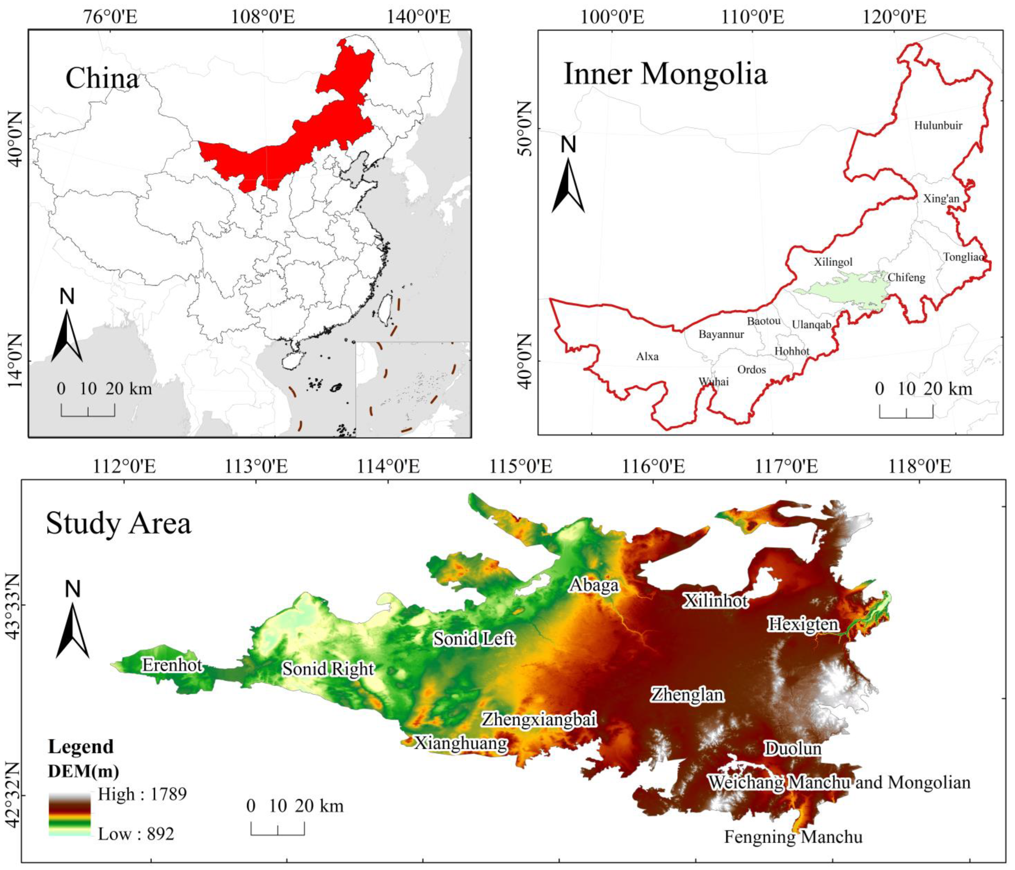
The research focused on the Hunshandake Sandy Land, one of the four principal sandy-land ecoregions in China and a key ecological shield for the Beijing–Tianjin–Hebei metropolis cluster (Figure 1). The sandy land extends primarily across Xilingol League in Inner Mongolia, with major distributions in Zhengblue Banner, Duolun County, Xilinhot City, Zhengxiangbai Banner, Abaga Banner, northern Xianghuang Banner, southern Sonid Left Banner, and central Sonid Right Banner. In addition, it partially extends into Chifeng City (Inner Mongolia) and Hebei Province (Figure 1).
Topographically, the terrain rises in the southwest and gently descends toward the northeast. The mean elevation is approximately 1300 m above sea level. The sandy land stretches roughly 400 km along an east–west axis, with a maximum north–south width of more than 120 km. Its geographical extent is bounded by 112°20′–117°50′ E longitude and 41°40′–43°10′ N latitude, covering an area of 4.27 × 10⁴ km2.
The region experiences a semi-arid climate, receiving 300–400 mm of mean annual precipitation, while evapotranspiration substantially exceeds precipitation, ranging from 1600 to 2900 mm. This imbalance between rainfall and evaporation underscores the region’s ecological fragility. Given its strategic role as a buffer zone for ecological security in North China, environmental changes in the Hunshandake Sandy Land are likely to exert cascading impacts on surrounding regions.

2.2. Data Sources

Here, we integrated land-use, meteorological, soil, elevation, NDVI, and socioeconomic datasets (Table 1). Together, these datasets provided the basis for quantifying ecosystem services (ESs) and assessing their spatial social–ecological drivers. Land use was categorized into eight classes: cropland, forest, high-, medium-, and low-coverage grassland, water bodies, urban land and fallow land. To secure comparability across datasets, all raster layers of differing spatial scales (Table 1) were unified to 30 m × 30 m by resampling.

2.3. Research Methodology

2.3.1. Ecosystem Services Assessment

To comprehensively evaluate ecosystem service (ES) performance across the Hunshandake Sandy Land and to inform evidence-based ecological management decisions, we assessed five key ESs: water conservation (WC), vegetation carbon sequestration (VS), biodiversity (BD), soil conservation (SC), and sand fixation (SF). Three modeling approaches were applied, encompassing the holistic valuation of ecosystem services and their trade-offs: the InVEST, CASA, and RWEQ models. WC was quantified as the pixel-level difference between yearly precipitation and observed ET, using the InVEST water-yield module based on the Budyko curve; VS was derived from NPP, which was estimated with the CASA model using vegetation indices. BD was maintained through habitat quality, which was quantified by the InVEST habitat-quality submodule. SC was calculated as the difference between potential (R × K × LS) and realized soil loss (R × K × LS × C × P) erosion using the RUSLE framework embedded in InVEST. SF was derived from the Revised Wind-Erosion Equation (RWEQ). All analyses were performed at 30 m spatial resolution for the five time slices: 2000, 2005, 2010, 2015, and 2020.

2.3.2. Correlation Analysis Between ES Pairs

To examine trade-offs and synergies between ESs, we first executed nonparametric associative assessment. Because geospatial data typically display nonlinear and non-normal distributions, Spearman’s rank correlation was selected as an appropriate nonparametric approach [13,31]. The analysis was based on n = 10.85 × 10⁷ independent sample plots (each a 30 m × 30 m pixel, spatially disjoint and treated as an independent observation). Correlation analyses were performed across five different times (2000, 2005, 2010, 2015, and 2020) with the R package corrplot (v4.4.1). Here, at ρ < 0.05, negative correlations signified trade-offs and positive correlations synergies, with the correlation magnitude indicating interaction strength.
To examine spatial heterogeneity in ES relationships, we applied Geographically Weighted Regression (GWR) beyond the pooled trade-off and synergy patterns, implemented utilizing the “GWmodel” package in R (v4.4.1) [12]. To mitigate local multicollinearity arising from high spatial autocorrelation in the original 30 m resolution data, the analysis was conducted at 1 km × 1 km grid resolution (n = 4.24 × 10 7 independent sample plots, each spatially disjoint and treated as an isolated observation), ensuring the statistical stability of the model outcomes. The GWR specification reads:
y i   =   β u i , v i + k = 1 p β k ( u i , v i ) d ik + ε i
where y i denotes ES at the i position, ( u i , v i ) is the geographic position of point i, β k is the k-th regression coefficient, d ik is the k-th predictor at grid cell i, and ε i is the error component.

2.3.3. Identification of ES Bundles

To visually illustrate and categorize geographic association patterns among multiple ESs, we implemented SOMs, a self-organizing neural-network approach that groups grid cells into clusters based on similarity [32]. A total of 174,668 grid cells covering Hunshandake Sandy Land across all study periods were exported as samples, and clustering of ES bundles was carried out via the Kohonen package (R 4.4.1).

2.3.4. Influences on Ecosystem Services

To investigate the impacts of environmental and socioeconomic drivers of ESs, we applied PLS-SEM. This framework combines pathway, factor, and regression analyses to estimate influence links between social–ecological drivers and ES [33]. PLS-SEM is especially well-suited to handling complex models with multiple constructs, limited sample sizes, and non-normal datasets distribution [34,35]. The PLS-SEM framework includes two components: the structural model, which defines the pathways among unobserved constructs, while the outer model, which defines the associations linking latent constructs to their observed indicators [36]. The general form of the equations to represent PLS-SEM is:
X   =   Λ x α +   β , Y   = Λ y λ   +   Φ
where X and Y represent latent factors and observed constructs, correspondingly, and Λ represents correlation relating to them.
Z = W × Z + N × £ + j
where Z and £ act as latent variables, N and W serve as their path coefficients, and j denotes the regression residual.
Here, six driving factors were selected: Digital elevation model (DEM), NDVI, ET, PRE, TMP, and GDP. Analyses were performed on a 1 km × 1 km grid using SmartPLS 4 software.

3. Results

3.1. Spatial–Temporal Variations of ESs

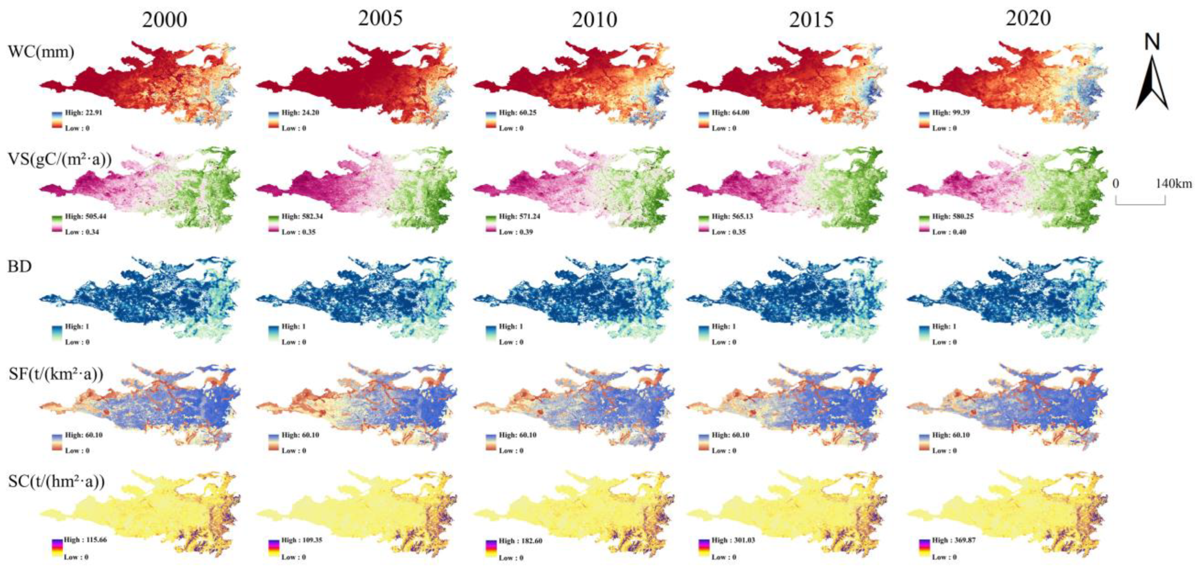
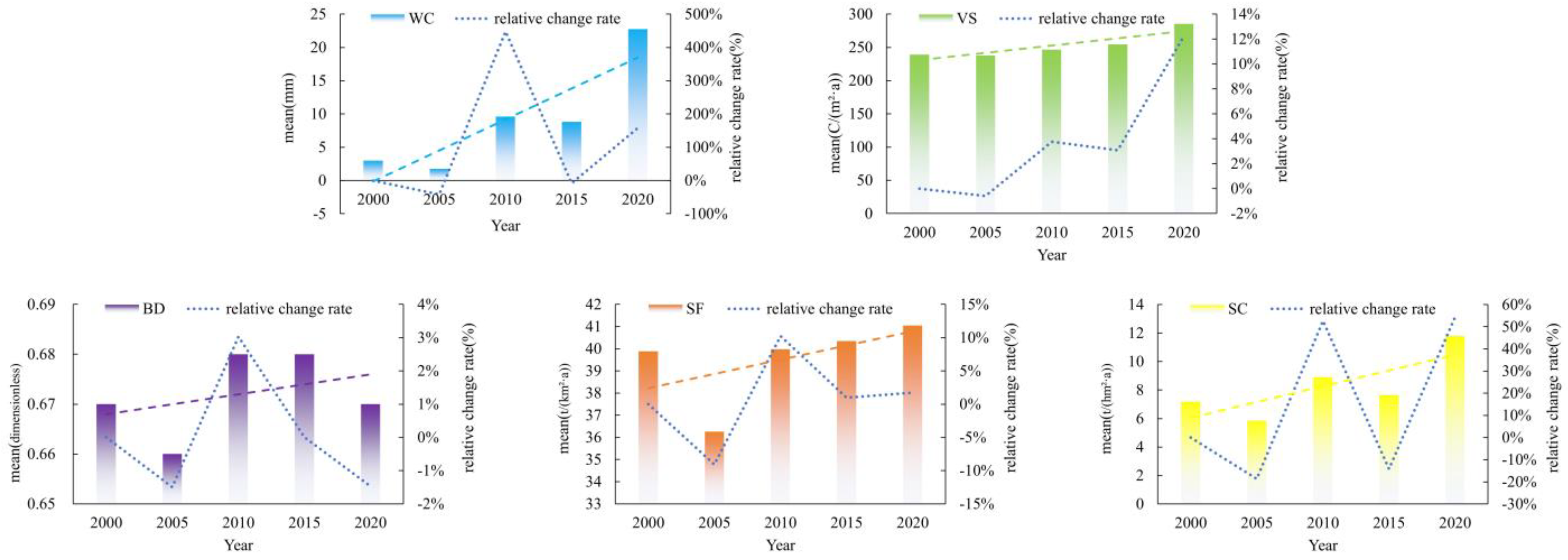
The spatial distributions of the five ecosystem services remained relatively stable between 2000 and 2020 (Figure 2). However, notable temporal dynamics were observed for individual services. For instance, the mean annual WC was 6.08 mm, with a fluctuating pattern, first declining and then increasing over the study period. The lowest WC capacity occurred in 2005, at 0.71 × 10⁸ m3, representing a decrease of 0.44 × 10⁸ m3 compared with 2000 and a decline of 1.04 mm in WC capacity. In contrast, WC peaked in 2020 at 5.68 × 10⁸ m3, an increase of 2.84 × 10⁸ m3 relative to 2015, with WC capacity rising by 6.65 mm. VS exhibited a slow but consistent upward trend, with an average annual level of 251.63 gC/(m2·a). The maximum value was recorded in 2020 (285.36 gC/(m2·a)), which was 13.40% above the annual mean, while the minimum occurred in 2005 (232.72 gC/(m2·a)), 7.51% below the mean.
BD remained relatively stable throughout the study period, with a mean annual index of 0.67 and no major interannual fluctuations. SF decreased from 2000 to 2005, followed by a gradual increase up to 2020. The mean annual value was 39.57 t/(km2·a). SF reached its highest value in 2020 at 41.13 t/(km2·a), while the lowest value was observed in 2005 at 36.34 t/(km2·a). The annual variation of SC exhibited periodic fluctuations of decreasing-increasing-decreasing-increasing, showing an overall double-trough, double-peak pattern with a mean annual value of 8.27 t/(hm2·a). SC reached its maximum value of 11.79 t/(hm2·a) in 2020, while the minimum value of 5.84 t/(hm2·a) occurred in 2005.
The distribution of ESs in the Hunshandake Sandy Land exhibited pronounced spatial heterogeneity (Figure 3). Each service exhibited distinct regional patterns shaped by bioclimatic and topographic factors, including precipitation regimes, elevation, soil organic matter, and vegetation cover. WC and VS showed broadly similar spatial patterns (east–west gradients), with elevated magnitudes focused across the wetter eastern region and diminished levels in the arid west. High-value zones included Duolun County, Zhenglan Banner, Hexigten Banner, Xilinhot City, and parts of Hebei Province, while Sonid Right Banner, Xianghuang Banner, and Erenhot City represented low-value areas.
For VS, high-value areas (annual mean > 300 gC/(m2·a)) were clustered in Duolun County, Zhenglan Banner, Hexigten Banner, and parts of Hebei Province, whereas low-value areas (annual mean < 200 gC/(m2·a)) were in Sonid Right Banner and Erenhot City. “From 2000 to 2020, VS increased most notably in Duolun County (104.61 gC/(m2·a)) and Hebei Province (199.54 gC/(m2·a)), with an average growth rate exceeding 5 gC/(m2·a). Most other regions grew more modestly (0–4 gC/(m2·a)).” BD high-value areas (annual mean > 0.85) were concentrated in Xianghuang Banner and Sonid Left Banner, representing 15.25% of the total study region. Conversely, low-value areas (annual mean < 0.38) occurred predominantly in Duolun County and parts of Hebei Province, occupying 7.04% of the total area. Across most regions, BD remained close to the mean, reflecting stability due to only minor short-term changes in land use structure.
SF followed an east–west gradient, with high-value areas in the eastern Hunshandake Sandy Land (Duolun County, Zhenglan Banner, Hexigten Banner, Xilinhot City) and low values in the west (Sonid Right Banner, Erenhot City). Between 2000 and 2005, marginal sandy areas expanded outward, encroaching on ecologically better transition zones. From 2005 to 2020, however, ecological governance measures curbed this expansion: marginal areas contracted inward, vegetation recovered, and ecological transition zones were restored and expanded. SC was highest in Duolun County (29.34 t/(hm2·a)), Hexigten Banner (24.23 t/(hm2·a)), and Hebei Province (27.81 t/(hm2·a)), while Sonid Right Banner (3.57 t/(hm2·a)) and Erenhot (2.47 t/(hm2·a)) represented low-value areas. From 2000 to 2020, SC increased significantly in Duolun County (19.08 t/(hm2·a)), Hexigten Banner (19.79 t/(hm2·a)), and Hebei Province (16.83 t/(hm2·a)), at an average rate exceeding 0.84 t/(hm2·a). These gains underscore the success of deployed soil and water retention interventions.

3.2. Trade-Offs and Synergies Between ES Pairs

3.2.1. Correlation Analysis

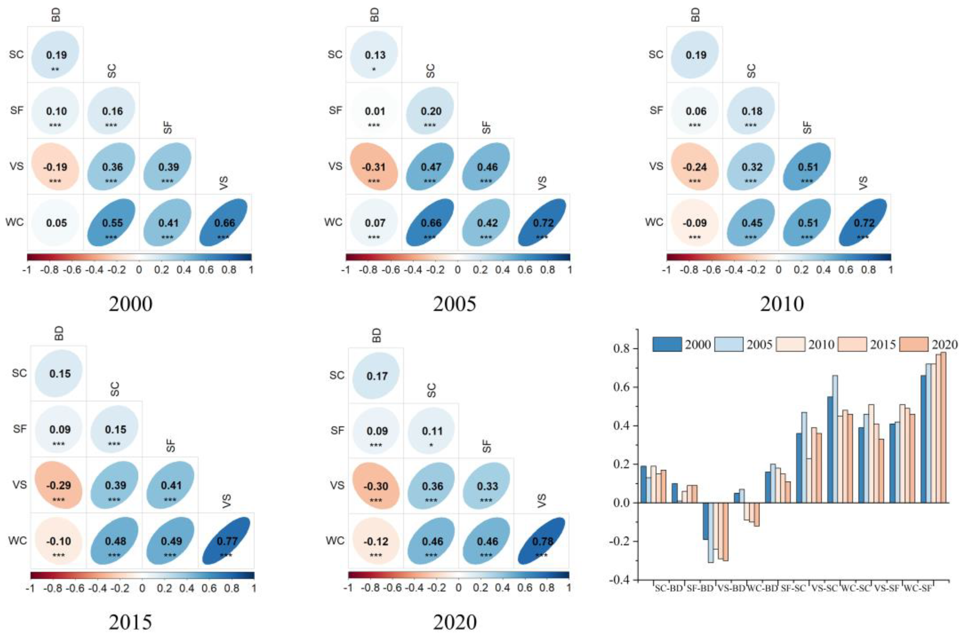
Spearman’s rank correlation coefficients were applied to assess pairwise relationships among the five ESs from 2000 to 2020, resulting in 10 unique ES pairs (Figure 4). All correlations were statistically significant (p < 0.001). The results revealed that most ES pairs exhibited positive correlations, indicating synergistic interactions, with only a few pairs showing negative correlations (i.e., trade-offs). The strongest trade-off emerged between VS and BD, which consistently displayed negative correlations throughout 2000–2020. This trade-off strengthened over time, reaching its lowest correlation coefficient of −0.31 in 2005, indicating a moderate negative relationship. During 2000–2005, the WC–BD pair showed a weak synergy; during 2010–2020, it shifted to a weak trade-off, with the correlation coefficient changing from 0.07 in 2005 to −0.12 in 2020. In contrast, several ES pairs demonstrated strong and persistent synergies. The WC–VS relationship was the most robust, with correlation coefficients exceeding 0.66 in both 2000 and 2020 and peaking at 0.78 by 2020. Other strong synergistic relationships included WC-SC (mean r = 0.52), VS-SF (mean r = 0.42), and WC-SF (mean r = 0.46). Moderate synergies were observed for VS-SC, SC-BD, and SF-SC, with correlation coefficients generally ranging from 0.1 to 0.4. In contrast, the SF-BD pair showed only a weak synergy, with correlation coefficients consistently below 0.1 and cropping to a minimum of 0.01 in 2005. Overall, Synergies among the five Ess attenuated over 20-year period, even for pairs that remained positively correlated. The most significant patterns were summarized as: (i) the VS-BD trade-off intensified over time, (ii) the WC-VS synergy remained prominent, (iii) the synergies of WC-SF and VS-SC gradually improved (“optimized”) despite an overall weakening trend across Ess, and (iv) the WC-BD relationship shifted from synergy to trade-off, reflecting changing ecological dynamics in the Hunshandake Sandy Land.

3.2.2. Spatial–Temporal Patterns of Trade-Offs and Synergies

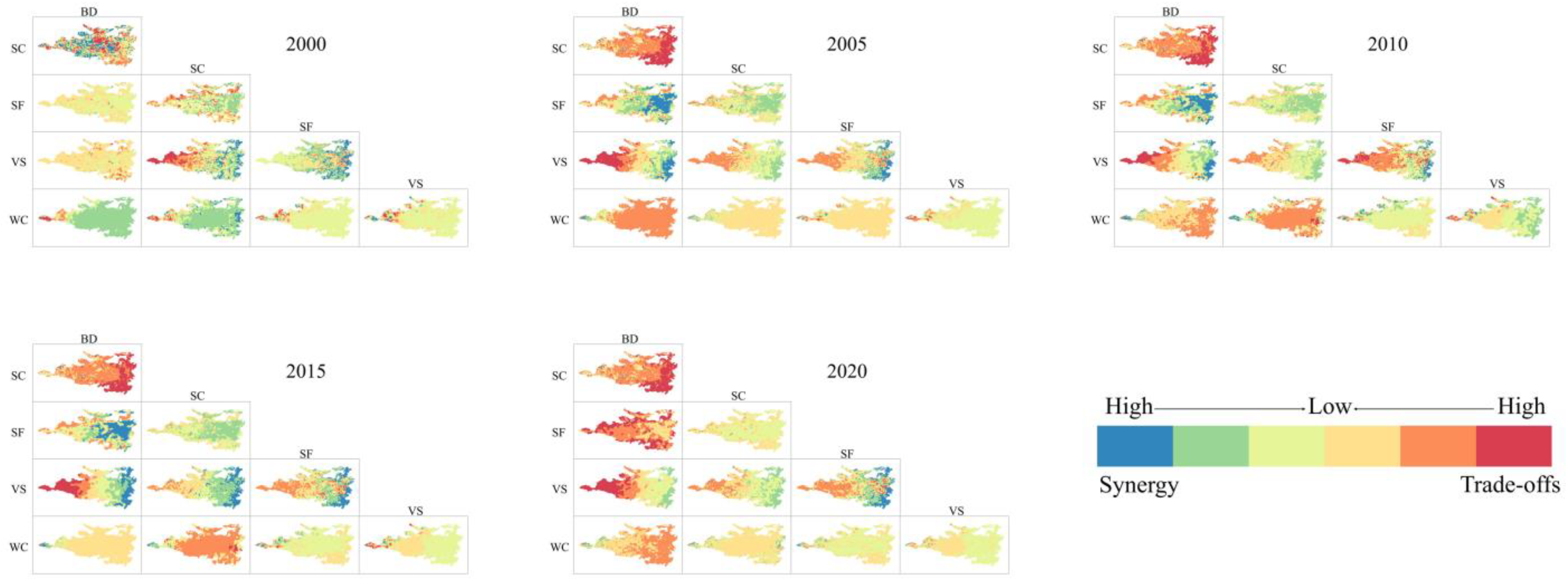
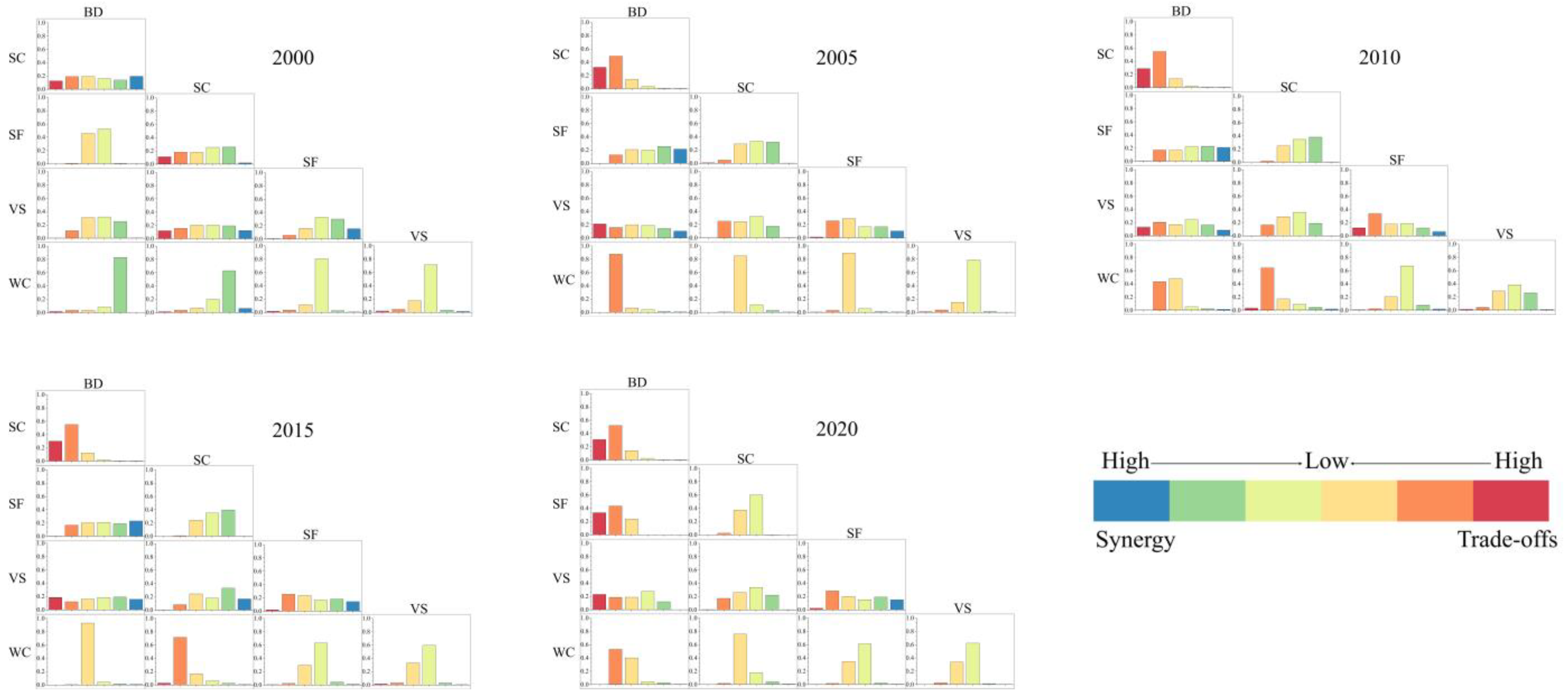
The GWR results demonstrated marked spatial heterogeneity in the trade-off and synergy effects of ES pairs throughout Hunshandake during the period 200–2020 (Figure 5). In 2000, ES pairs involving WC showed strong spatial synergies, especially in the central and eastern areas (Figure 5). By 2020, WC-BD and WC-SC shifted to strong spatial trade-offs, while WC-SF and WC-VS transitioned to weak synergies. For SC-BD, spatial trade-offs and synergies were initially balanced in 2000, but from 2005 onward, the relationship shifted toward strong and widely distributed trade-offs (Figure 6). Results also revealed that SF-SC and VS-SC maintained slightly larger synergistic areas than trade-off areas, and their spatial configurations stayed largely unchanged through time. In contrast, SF-BD and VS-BD gradually transitioned from weak trade-offs to strong trade-offs, with a significant expansion of their trade-off areas in the western region. The VS-SF pair exhibited a more balanced pattern, with both high trade-offs and high synergies coexisting across the entire study timeframe.

3.3. Spatial–Temporal Patterns of ESs

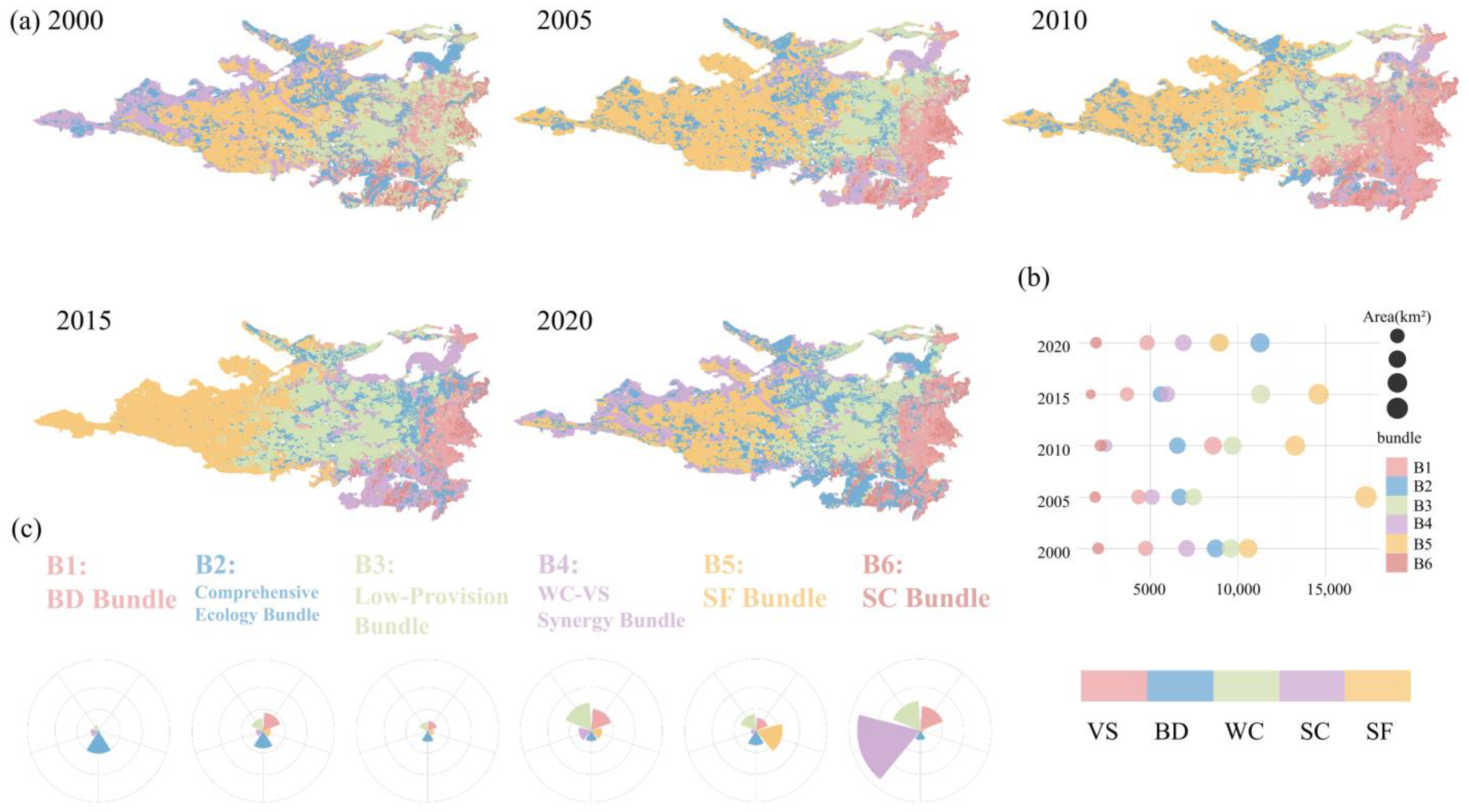
The SOMs analysis identified six ESBs, each representing a distinct combination of ES supply levels (Figure 7). The six ESBs represented as B1 (BD bundle), with high BD but very low supply of other ESs, indicating relatively intact ecological functions; B2 (comprehensive ecology bundle), with balanced supply of all ESs; B3 (low-provision bundle) with low supply of all ESs, reflecting low overall ecosystem capacity; B4 (WC-VS synergy bundle), with high WC and VS, indicating abundant water, extensive vegetation cover, and high carbon storage, but low BD, SC, and SF; B5 (SF bundle), with high SF, indicating strong sand-fixation capacity; and B6 (SC bundle), with high SC, reflecting strong resistance to soil erosion.
Across the temporal scale (i.e., from 2000 to 2010), the areas of B1, B3, B5, and B6 expanded, while B2 and B4 contracted. From 2010 to 2020, this trend reversed, with B2 and B4 expanded and B1, B3, B5, and B6 shrunk. Spatially, B1 and B6 were concentrated mainly in the east, B2 and B3 were centered in the central region of the study area, the distribution of B4 changed over time, gradually shifting from the western part to the eastern part and then back to the western part, and B5 was consistently dominant in the west.

3.4. Drivers of Ecosystem Service Functionality

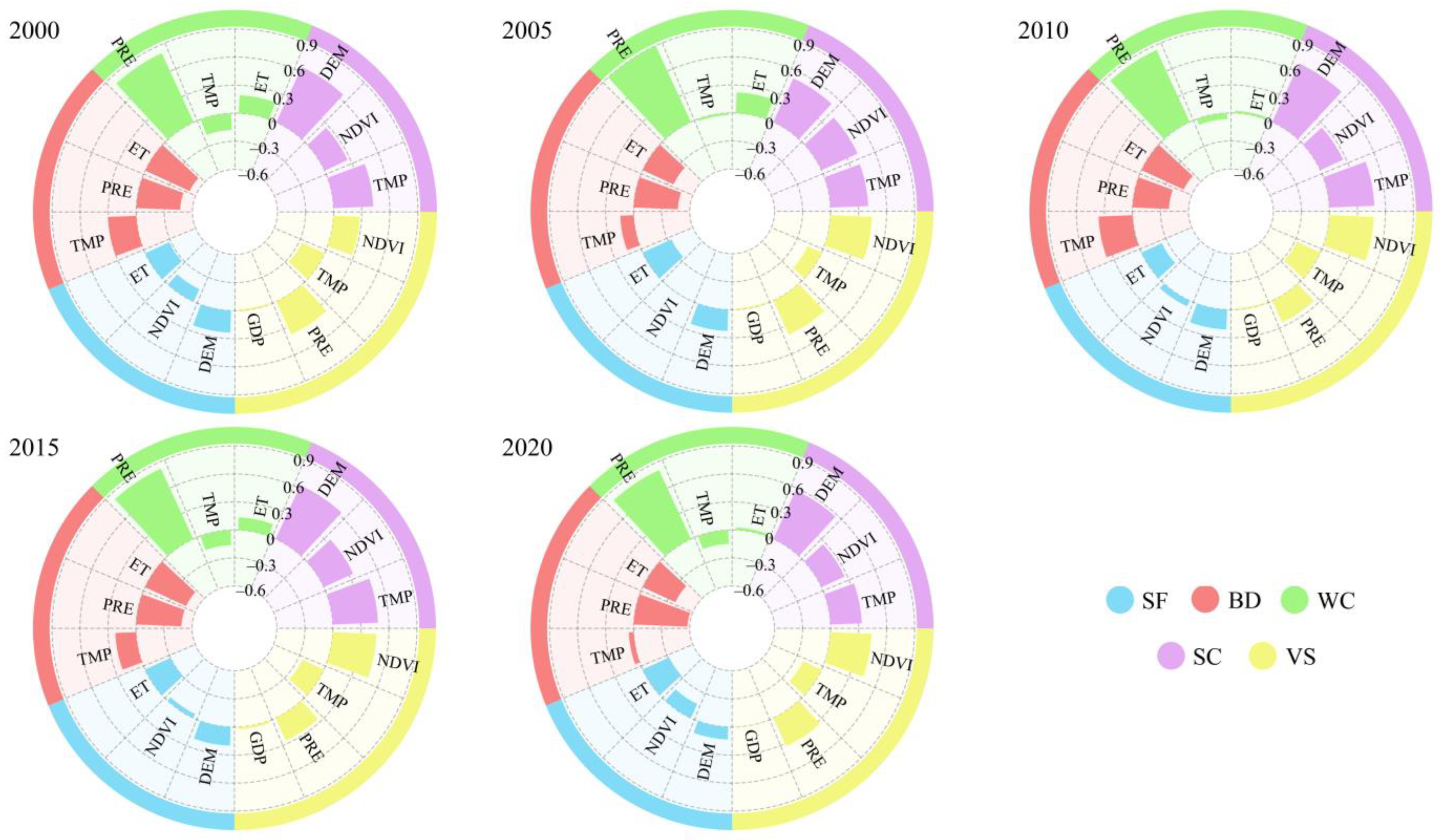
The temporal changes in path coefficients between ESs and their drivers from 2000 to 2020 highlighted the marked variation in both the direction and magnitude of services and years (Figure 8, Table 2). For SF, DEM exerted the strongest positive influence, although its effect declined from 0.236 in 2000 to 0.134 in 2020. The NDVI showed a non-linear pattern, shifting from negative to positive and back to negative over time. ET consistently showed a strong inhibitor, and with the most negative coefficient in 2005 (−0.339). BD was highly sensitive to climatic variations. Both PRE and ET exhibited significant negative correlations throughout the study period, with PRE showing the strongest negative effect in 2020 (−0.576) and ET in 2000 (−0.522). In contrast, TMP showed a fluctuating positive effect, peaking in 2010 (0.364). For WC, PRE consistently exerted a strong positive effect (all path coefficients > 0.81) and peaked in 2005 (0.902). TMP remained negatively correlated with WC across all years, with the strongest negative effect in 2015 (−0.161). ET showed a weaker, generally positive influence.
SC was primarily driven by DEM and NDVI, underscoring the importance of stable topography and vegetation cover. DEM influence peaked in 2010 (0.689), while NDVI reached its maximum effects in 2005 (0.425). TMP effects were small and inconsistent. For VS, NDVI was the key positive driver, with its path coefficient increasing from 0.279 in 2000 to 0.477 in 2010, before slightly declining thereafter. TMP exerted a persistent negative effect, whereas PRE had a moderate positive effect. GDP showed weak and inconsistent effects, suggesting minimal socioeconomic control over VS during the study period.
Overall, our results highlighted that PRE, as a dual force driver, strongly enhancing WC but suppressing BD. TMP generally exerted mild negative effects across most services, while DEM was key for SC and SF, but with a declining influence over time. NDVI showed a positive influence on VS and SC, especially during 2005–2010, before weakening. ET consistently inhibited multiple services, indicating potential risks from warming and increased water consumption in the future.

4. Discussion

4.1. Characteristics of Ecosystem Service Interactions

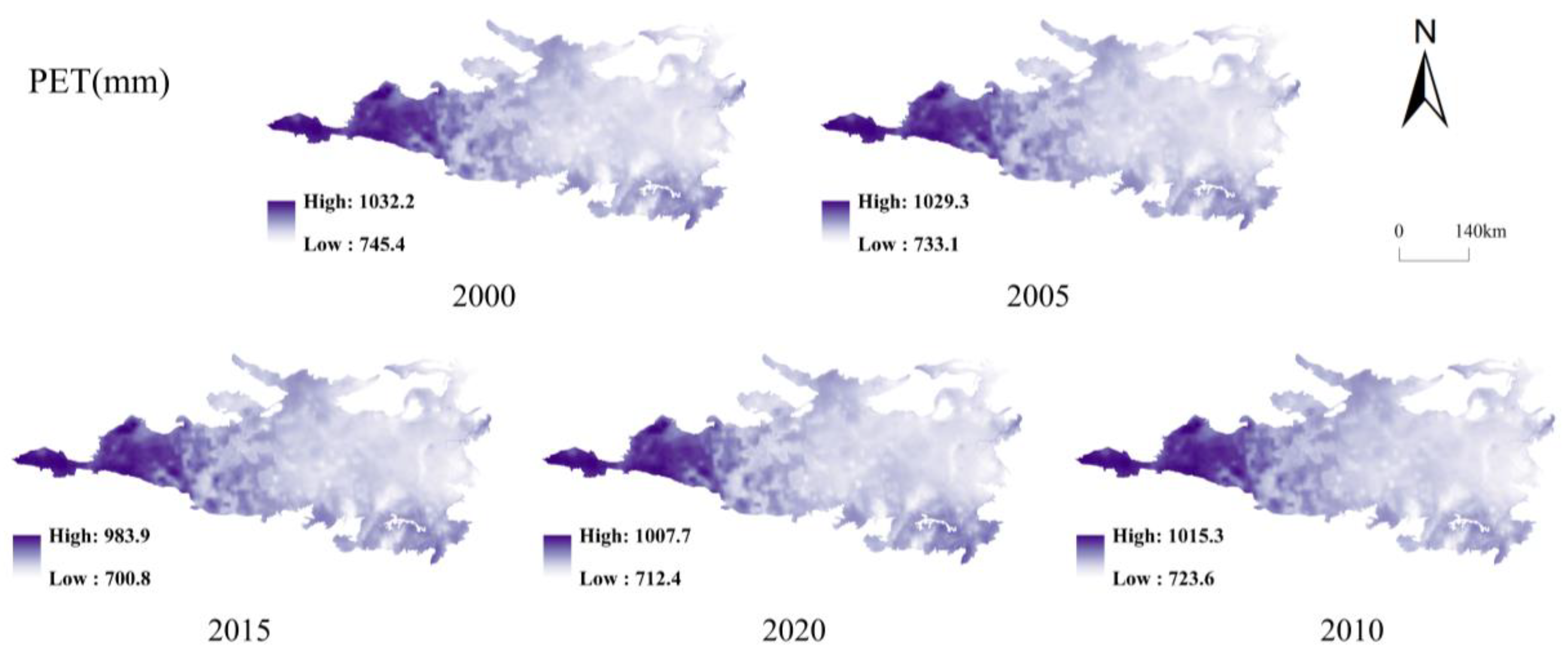
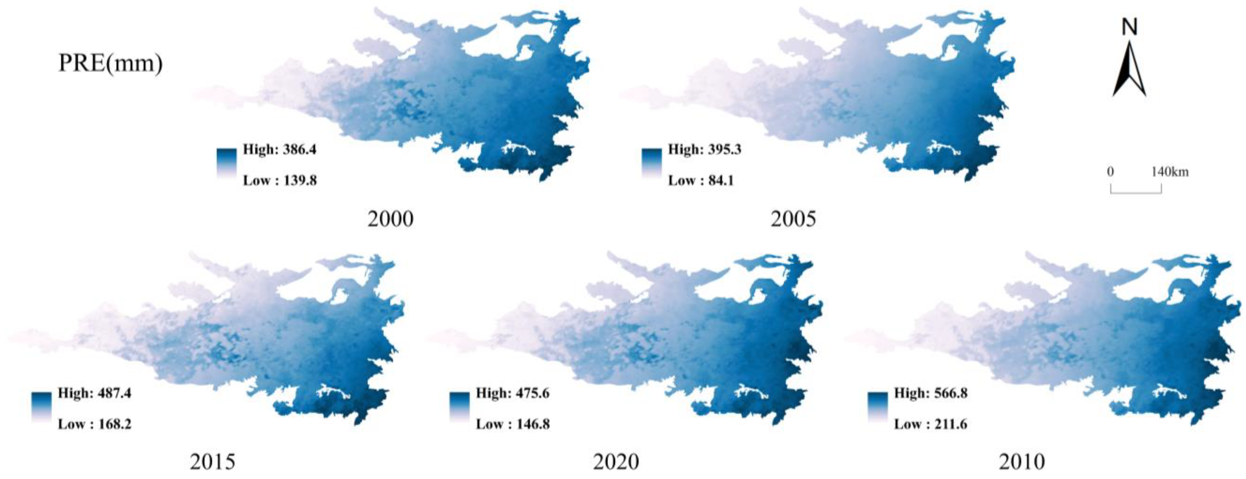
The spatial patterns of ESs in the Hunshandake Sandy Land revealed clear east–west gradients, reflecting strong climatic and land-use controls. Among the five ESs, WC, VS, SC, and SF displayed comparable spatial configurations: elevated values dominated the east, whereas diminished levels prevailed in the west, aligning with earlier studies. (Wang [30]). In contrast, BD displayed a more fragmented and discrete pattern across the landscape. This spatial differentiation aligns closely with regional hydrology and climatic conditions. Annual precipitation in the eastern Hunshandake Sandy Land ranges from 300 to 400 mm (Figure 9), with actual evapotranspiration matching potential evapotranspiration, creating favorable conditions for vegetation growth. In contrast, the western region receives <200 mm of precipitation, while potential evapotranspiration can reach 700–1100 mm (Figure 10), producing a pronounced water deficit that limits plant cover. Vegetation cover showed a strong positive relationship with soil-water storage depth in both grasslands and forests, likely because denser vegetation curbs surface runoff and enhances infiltration into deeper soil layers [37]. Land use patterns further reinforce these gradients. Grasslands dominate the landscape, covering 69.8% of the area and primarily distributed across the central and northern regions, with cropland (10.8%) and forest (8.6%) as secondary types [38], which cluster mainly in the south-west and south-east [39]. The eastern region of the study area supports a mixed agricultural–pastoral economy, whereas the central and western regions are largely pastoral [29]. Grasslands in the east are characterized by temperate bunchgrass steppe, sparse forest, and shrubland with high vegetation cover, reflecting successful ecological restoration. In contrast, the western regions are dominated by semi-mobile and mobile dunes and sparse vegetation cover, with severe degradation [40]. High BD values were concentrated in grasslands and woodlands with dense vegetation cover. In contrast, low BD values occurred mainly in croplands, built-up areas, and unused lands, resulting in a highly fragmented BD patch pattern and underscoring land use as a key driver of habitat quality [41].
Temporal dynamics reveal these spatial patterns. From 2000 to 2005, most ES functions declined, followed by stabilization and partial recovery during 2005–2010, and a marked increase between 2010 and 2020. The early decline was driven by consecutive droughts (1999–2002) and severe overgrazing, which accelerated vegetation degradation and grassland fragmentation. Vegetation recovery began after 2005, supported by enclosure fencing, rotational grazing, and afforestation programs, which curbed degradation and promoted regrowth. From 2010 onward, stronger ecological policies, including the “Grain-for-Green” restoration scheme and the grassland ecological-compensation incentive, further enhanced restoration, culminating in a 420 km × 1–10 km ecological shelterbelt along the southern margin of the sandy land. The temporal dynamics of ecosystem services in the Hunshandake Sandy Land from 2000 to 2020 revealed a distinct pattern of initial decline, stabilization, and subsequent marked recovery. This trajectory was primarily driven by a shift from early climatic stressors and overgrazing to later, intensive ecological restoration policies. These findings align with the restoration trajectories reported by Liu [29]. The consistency strongly reinforces a key consensus in dryland ecology: sustained, large-scale human intervention through targeted policies (e.g., grazing exclusion, afforestation) can effectively reverse ecosystem degradation and enhance multiple ESs, even in fragile sandy land ecosystems. Both studies highlight the critical turning point around 2005–2010, linking recovery to nationwide ecological programs such as “Grain-for-Green” and the “Grassland Ecological Compensation Policy”. This alignment confirms that policy-driven restoration is a dominant and reproducible driver of ecological improvement at the regional scale in northern China.

4.2. Ecosystem Service Trade-Off, Synergy, and Bundles Analysis

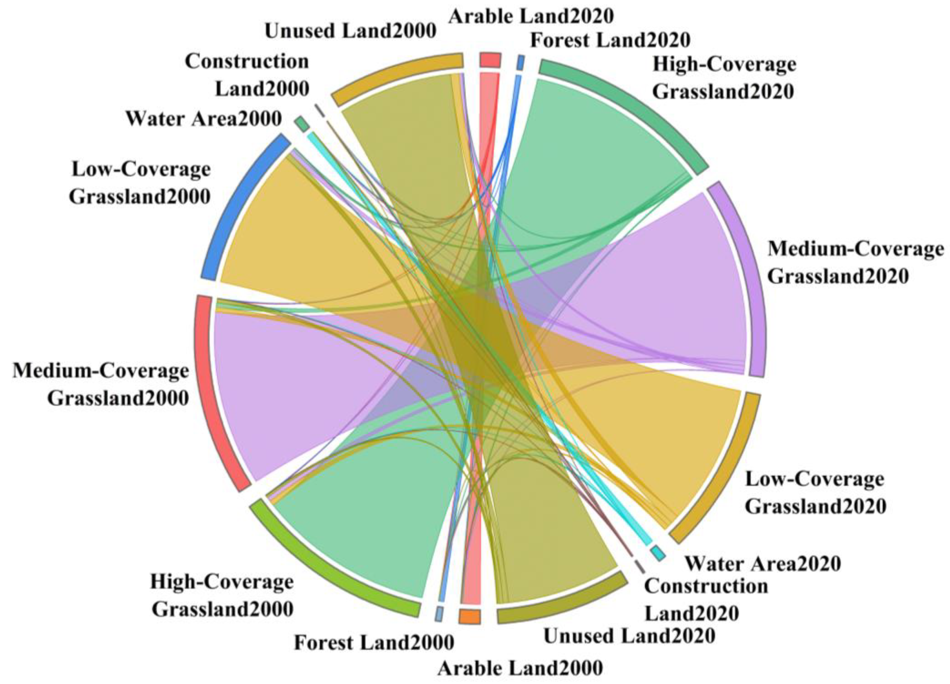
Land-cover transitions are a primary driver of ES trade-offs and synergies, making their characterization essential for ecosystem management and policy design. To capture these dynamics, a land-cover transition matrix was developed for the Hunshandake Sandy Land to quantify mutual conversions among arable land, forest land, high-cover, medium-cover and low-cover grassland, water area, built-up land and unused land that prevailed from 2000 to 2020. Our analyses revealed that land-use dynamics across the two decades were strongly shaped by ecological restoration programs, particularly the “Grain for Grass” policy. Between 2000 and 2020, 8.18% of arable land was converted to grassland, reflecting deliberate efforts to reduce cultivation and enhance vegetation cover. Within grassland types, conversions favored ecological improvement: 5.36% of grasslands were transformed into high-coverage grassland, 3.10% into medium-coverage grassland, while only 0.71% degraded to unused land. Medium-coverage grassland underwent both upward and downward shifts, with 300.10 km2 converted to low-coverage grassland and an additional 286.41 km2 experiencing similar degradation. Changes were less pronounced in other land types. Water bodies remained relatively stable, with unused land showing notable ecological recovery, with a substantial area converted to grassland. Among these conversions, transformation to low-coverage grassland was most significant, covering 514.83 km2 (6.53% of the total area) (Figure 11).
Across the study region, most ecosystem-service pairs exhibited synergistic relationships, with particularly strong positive synergy between WC and VS (r = 0.66 in 2000, r = 0.78 in 2020). The pair’s synergy was spatially dominant across the central and eastern parts. Synergies between WC–SC and WC–SF remained comparatively stable, with correlation coefficients consistently ranging from 0.4 to 0.6. Enhanced WC increases vegetation cover and reduces surface-runoff coefficients, thereby alleviating drought stress. In turn, higher canopy interception and litter-water-storage capacity expands the soil carbon and nitrogen pool, generating a positive feedback loop in which elevated WC enhances soil moisture, which in turn boosts VS. These statements are consistent with Yang et al. [42], who reported that higher water availability supports vegetation cover, increasing root biomass and surface roughness, reducing near-surface wind speed, and trapping more sediment. Consequently, sandstorm prevention and soil retention services are simultaneously improved [29]. In this study, the WC–VS positive feedback further increases surface roughness and the threshold wind velocity for sand entrainment, reduces aeolian erosion, and enhances soil cohesion, thereby jointly amplifying SF and SC. Collectively, these relationships underscore WC as an indispensable component of regional ecological security, sustaining land productivity in arid zones and fostering long-term ecosystem sustainability.
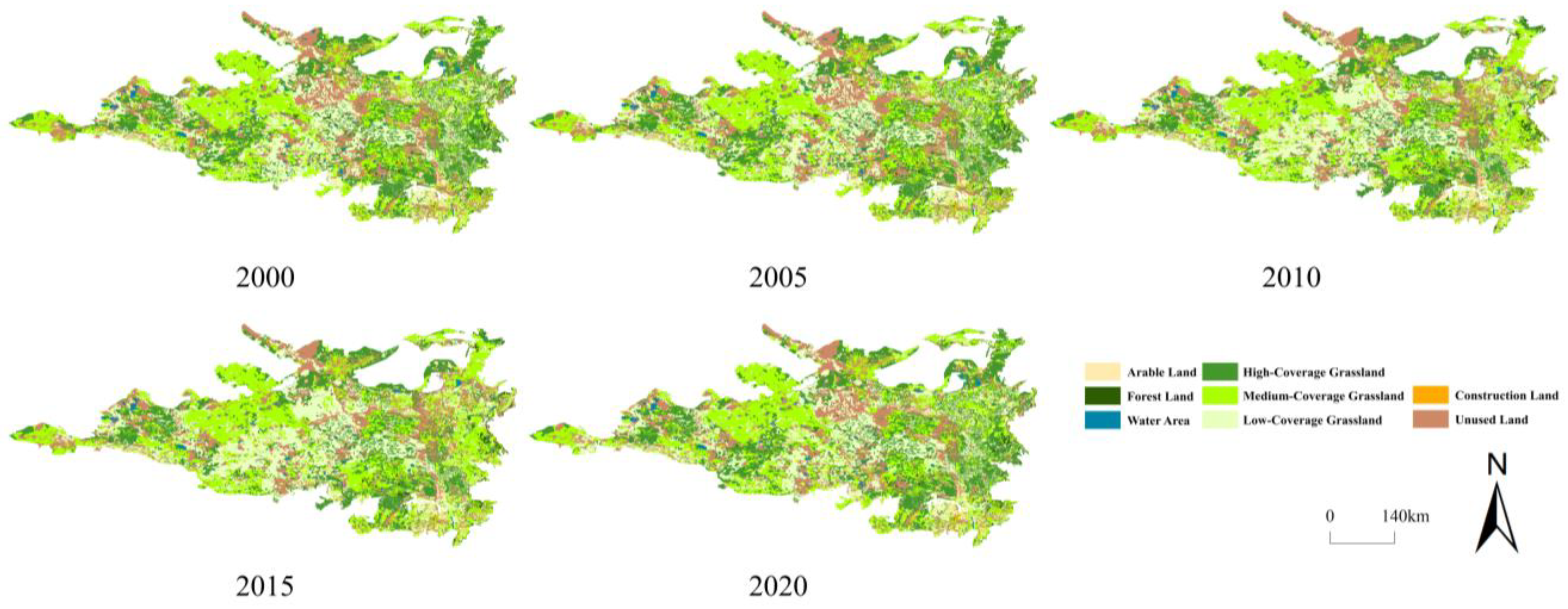
In contrast, a pronounced trade-off emerged between VS and BD. Over the past two decades, large-scale afforestation and cropland expansion have replaced the original grassland–shrubland–sand mosaic with homogeneous, high-productivity patches (Figure 12, Table 3). This outcome diverges from reports in mesic biomes, where afforestation often enhances both carbon sequestration and habitat diversity in the early stages. For example, mixed-species reforestation in subtropical China simultaneously increased vegetation carbon by 28% and plant species richness by 15% within the first ten years [43]. In the Hunshandake Sandy Land, fertilised or fast-growing-seeded plantations rapidly increase aboveground biomass but simultaneously reduce habitat quality for native perennial forbs and cryptogams, leading to a significant decline in BD. VS can be quickly elevated through dense planting or aerial seeding, whereas BD recovery relies on slow, long-term successional processes. As restoration strategies shifted from “moderate revegetation” to dense artificial planting, the WC–BD relationship transitioned from synergy to trade-off. Late-stage sand-fixation projects frequently adopt fast-growing species such as Pinus sylvestris var. mongolica, which immediately enhance canopy interception and root water retention but also double evapotranspiration rates and displace key steppe indicator species, thereby accelerating BD loss. These results highlight that managing the VS–BD and WC–BD trade-offs is critical for sustainable ecosystem recovery in the Hunshandake Sandy Land. Balancing rapid vegetation stabilization with the slower processes of biodiversity regeneration is essential for maintaining both ecological integrity and long-term resilience.
Across the Hunshandake Sandy Land, six functional clusters were delineated, each with distinct ecological characteristics and management priorities: B1 recorded the highest aggregate biodiversity-service value and was extensively distributed in the east. This high-diversity Ulmus woodland system provides strong buffering capacity against anthropogenic disturbance and is therefore suitable for low-density, conservation-oriented development. B2 exhibited a balanced distribution of all ecosystem services and occurred as an expanding, patchy mosaic in the central region. Its structural elasticity supports light, decentralized utilization under carefully regulated, fine-grained management. B3 was characterized by uniformly low service contributions, warranting a management approach of “natural recovery first, minimal intervention second” to promote near-natural, low-density restoration. B4 represented a scattered but proportionally small WC–VS synergistic bundle. This cluster requires strict protection to allow spontaneous outward expansion, which could catalyze a broader regional functional upgrade. B5 was dominated by sand-fixation services, extensively distributed in the west. With a high elasticity threshold to wind stress, it serves as the core zone for “sand-source prevention and sustainable resource utilization”. B6 was dominated by soil-conservation services, extensively distributed in the east but occupying the smallest proportional area, which should be managed with light, low-intensity use that maintains continuous grass cover to safeguard and sustain soil-conservation benefits. These functional clusters provide a spatially explicit framework for tailoring ecosystem management—ranging from strict protection and passive restoration to controlled utilization—thereby supporting both ecological security and sustainable land use across the Hunshandake Sandy Land.

4.3. Implications of Driving Factors for Ecosystem Services

The dynamic trajectory of path coefficients from 2000 to 2020 demonstrated that ES trade-offs in the Hunshandake Sandy Land are not static; instead, they shift sequentially driven by the combined effects of climate, landform, vegetation, and human drivers. Among these drivers, precipitation exhibited the strongest and most consistent influence, maintaining a dominant positive effect on water conservation (β > 0.81) but a significant negative effect on habitat quality (β < −0.40). This pattern indicates a climate-induced lock-in of the water–biodiversity trade-off, where gains in WC come at the expense of BD. Vegetation greenness, represented by NDVI, positively influenced SC and VS, with peak effects observed during 2005–2010 (β = 0.425–0.477). However, these coefficients have since declined, indicating that the initial gains from ecological-engineering projects have weakened as forests and grasslands entered a successional plateau. Similarly, the path coefficients of elevation on SF and SC declined by 43% over two decades, implying a diminishing role of topographic factors as intensifying land-use activities increasingly dominate ecosystem dynamics. A monitoring transect from Yan’an to Yulin on the Chinese Loess Plateau revealed that after the “Grain-for-Green” program (2000–2015), the marginal gains in soil conservation (SC) and carbon sequestration (CS) dropped sharply once NDVI exceeded 0.35, with standardized path coefficients declining from 0.46 to 0.18. This trajectory mirrors the post-peak downturn observed in the Hunshandake Sandy Land after 2005–2010, underscoring that once forests and grasslands enter a successional plateau, the scope for further ES enhancement narrows markedly. The parallel attenuation of ecosystem-service gains observed in the Hunshandake Sandy Land and on the Chinese Loess Plateau is underpinned by a common ecological threshold. Both regions are characterised by open elm-dominated woodlands that rapidly establish a projected foliage cover equivalent to NDVI ≈ 0.35. At this level, canopy interception and root reinforcement already neutralise most rainfall erosivity, while stand-level net primary productivity approaches a steady state because soil-water availability becomes the prevailing constraint under semi-arid precipitation (380–450 mm). Consequently, the marginal increments of soil conservation and carbon sequestration decline synchronously, confirming that the transition from active establishment to a water-limited successional plateau—not taxonomic composition—governs the post-restoration ES trajectory across dryland China. Notably, evapotranspiration emerged as a growing constraint, with its negative coefficients for both SF and BD strengthening over time. This trend underscores the amplifying impact of warming-induced evapotranspiration pressure on ecosystem vulnerability and trade-off risks. In this context, eco-compensation mechanisms—already effective at aligning economic incentives with ecological conservation in transboundary watersheds [44], offering a promising model for balancing development and restoration. Future ecosystem stewardship in the Hunshandake Sandy Land should establish a dynamic, self-adaptive regulation system that integrates technological innovation, policy reform, and community participation. Such an approach would proactively govern ES trade-offs and deliver the triple dividend of ecological conservation, economic development, and livelihood improvement.

4.4. Limitations and Future Prospects

This study, to our knowledge, provides the first comprehensive analysis of ES bundles in the Hunshandake Sandy Land, offering new insights into spatial interactions among services. However, the study also has several limitations: (1) Ecosystem processes are inherently complex, and the correction coefficients used in simulations carry uncertainties that may restrict the precision of ES quantification. Future research could incorporate Bayesian inference or machine learning techniques to achieve annual dynamics inversion, thereby reducing prior parameter errors and improving model reliability. (2) The study lacks the other service coverage, such as cultural services, and including cultural and recreational dimensions in future research would provide a more holistic understanding of ecosystem value. (3) Although key drivers of individual ES functions were identified, future studies should further explore the drivers of ES trade-offs, synergies, and ES bundles, which are critical for designing adaptive management strategies.

5. Conclusions

Using a multi-model framework, this study simulated five key ESs and analyzed their spatial interactions, bundles, and drivers in the Hunshandake Sandy Land. ESs patterns exhibited strong spatial variability but remained relatively stable over time. Positive interactions were most pronounced among WC, BD, and VS, with synergistic clusters concentrated in the arid western region. We identified six ES bundles. Between 2000 and 2020, the areas of B1, B3, B4, and B5 remained relatively stable, while B2 expanded and B6 contracted. The dominant drivers of each ES differed, underscoring the need for context-specific management strategies. These findings highlight a tiered management framework that leverages identified trade-offs, synergies, and bundle distributions to guide policy and restoration efforts. Based on the identified VS–BD and WC–BD trade-offs, we recommend establishing mixed-species shrub belts and seasonal grazing enclosures in the western arid cluster (B2) before 2030, to convert current trade-offs into synergies and simultaneously enhance carbon sequestration, habitat quality and long-term ecological resilience. Such strategies will be critical to achieving the sustainable development in the Hunshandake Sandy Land, ensuring long-term ecological resilience while supporting human well-being.

Author Contributions

Conceptualization, X.K., J.S. and H.L.; methodology, X.K.; software, X.K.; writing—original draft, X.K.; writing—review and editing, X.K. and H.L.; writing—original draft preparation, J.S.; investigation, J.S.; resources, H.L.; supervision, Y.H. All authors have read and agreed to the published version of the manuscript.

Funding

This research was funded by the ‘open bidding for selecting the best candidates’ project of Inner Mongolia Autonomous Region (grant number 2024JBGS0010), the Inner Mongolia Autonomous Region Water Conservancy Science and Technology Project (grant number NSK202408), the Inner Mongolian Natural Science Foundation of China (grant number 2024MS04016) and the Project of Key Laboratory of River and Lake in Inner Mongolia Autonomous Region (2025KYPT0020).

Institutional Review Board Statement

Not applicable.

Informed Consent Statement

Not applicable.

Data Availability Statement

The original contributions presented in this study are included in this article. Further inquiries can be directed to the corresponding authors.

Conflicts of Interest

The authors declare no conflicts of interest.

References

  1. Millennium Ecosystem Assessment (Ed.) Ecosystems and Human Well-Being: Synthesis; The Millennium Ecosystem Assessment Series; Island Press: Washington, DC, USA, 2005; ISBN 978-1-59726-040-4. [Google Scholar]
  2. Costanza, R.; d’Arge, R.; de Groot, R.; Farber, S.; Grasso, M.; Hannon, B.; Limburg, K.; Naeem, S.; O’Neill, R.V.; Paruelo, J.; et al. The Value of the World’s Ecosystem Services and Natural Capital. Ecol. Econ. 1998, 25, 3–15. [Google Scholar] [CrossRef] [Scilit]
  3. Dong, W.; Wu, X.; Zhang, J.; Zhang, Y.; Dang, H.; Lü, Y.; Wang, C.; Guo, J. Spatiotemporal Heterogeneity and Driving Factors of Ecosystem Service Relationships and Bundles in a Typical Agropastoral Ecotone. Ecol. Indic. 2023, 156, 111074. [Google Scholar] [CrossRef] [Scilit]
  4. Ginoux, P.; Prospero, J.M.; Gill, T.E.; Hsu, N.C.; Zhao, M. Global-scale Attribution of Anthropogenic and Natural Dust Sources and Their Emission Rates Based on MODIS Deep Blue Aerosol Products. Rev. Geophys. 2012, 50, 2012RG000388. [Google Scholar] [CrossRef] [Scilit]
  5. Humphrey, V.; Zscheischler, J.; Ciais, P.; Gudmundsson, L.; Sitch, S.; Seneviratne, S.I. Sensitivity of Atmospheric CO2 Growth Rate to Observed Changes in Terrestrial Water Storage. Nature 2018, 560, 628–631. [Google Scholar] [CrossRef] [Scilit]
  6. Bestelmeyer, B.T.; Okin, G.S.; Duniway, M.C.; Archer, S.R.; Sayre, N.F.; Williamson, J.C.; Herrick, J.E. Desertification, Land Use, and the Transformation of Global Drylands. Front. Ecol Environ. 2015, 13, 28–36. [Google Scholar] [CrossRef] [Scilit]
  7. Gao, J.; Zuo, L. Revealing Ecosystem Services Relationships and Their Driving Factors for Five Basins of Beijing. J. Geogr. Sci. 2021, 31, 111–129. [Google Scholar] [CrossRef] [Scilit]
  8. Gonzalez-Ollauri, A.; Mickovski, S.B. Providing Ecosystem Services in a Challenging Environment by Dealing with Bundles, Trade-Offs, and Synergies. Ecosyst. Serv. 2017, 28, 261–263. [Google Scholar] [CrossRef] [Scilit]
  9. Bennett, E.M.; Peterson, G.D.; Gordon, L.J. Understanding Relationships among Multiple Ecosystem Services. Ecol. Lett. 2009, 12, 1394–1404. [Google Scholar] [CrossRef] [Scilit]
  10. Raudsepp-Hearne, C.; Peterson, G.D.; Bennett, E.M. Ecosystem Service Bundles for Analyzing Tradeoffs in Diverse Landscapes. Proc. Natl. Acad. Sci. USA 2010, 107, 5242–5247. [Google Scholar] [CrossRef] [Scilit]
  11. Kong, L.; Zheng, H.; Xiao, Y.; Ouyang, Z.; Li, C.; Zhang, J.; Huang, B. Mapping Ecosystem Service Bundles to Detect Distinct Types of Multifunctionality within the Diverse Landscape of the Yangtze River Basin, China. Sustainability 2018, 10, 857. [Google Scholar] [CrossRef] [Scilit]
  12. Xia, H.; Yuan, S.; Prishchepov, A.V. Spatial-Temporal Heterogeneity of Ecosystem Service Interactions and Their Social-Ecological Drivers: Implications for Spatial Planning and Management. Resour. Conserv. Recycl. 2023, 189, 106767. [Google Scholar] [CrossRef] [Scilit]
  13. Lyu, R.; Clarke, K.C.; Zhang, J.; Feng, J.; Jia, X.; Li, J. Spatial Correlations among Ecosystem Services and Their Socio-Ecological Driving Factors: A Case Study in the City Belt along the Yellow River in Ningxia, China. Appl. Geogr. 2019, 108, 64–73. [Google Scholar] [CrossRef] [Scilit]
  14. Yu, H.; Jiang, J.; Gu, X.; Cao, C.; Shen, C. Using Dynamic Bayesian Belief Networks to Infer the Effects of Climate Change and Human Activities on Changes in Regional Ecosystem Services. Ecol. Indic. 2025, 170, 113023. [Google Scholar] [CrossRef] [Scilit]
  15. Wang, Y.; Ang, Y.; Zhang, Y.; Ruan, Y.; Wang, B. Identification of Ecological Functional Areas and Scenario Simulation Analysis of the Wanjiang Urban Belt from a Trade-Off/Synergy Perspective. Land 2025, 14, 444. [Google Scholar] [CrossRef] [Scilit]
  16. Zuo, L.; Gao, J. Investigating the Compounding Effects of Environmental Factors on Ecosystem Services Relationships for Ecological Conservation Red Line Areas. Land Degrad. Dev. 2021, 32, 4609–4623. [Google Scholar] [CrossRef] [Scilit]
  17. Zheng, D.; Wang, Y.; Hao, S.; Xu, W.; Lv, L.; Yu, S. Spatial-Temporal Variation and Tradeoffs/Synergies Analysis on Multiple Ecosystem Services: A Case Study in the Three-River Headwaters Region of China. Ecol. Indic. 2020, 116, 106494. [Google Scholar] [CrossRef] [Scilit]
  18. Sasaki, K.; Hotes, S.; Ichinose, T.; Doko, T.; Wolters, V. Hotspots of Agricultural Ecosystem Services and Farmland Biodiversity Overlap with Areas at Risk of Land Abandonment in Japan. Land 2021, 10, 1031. [Google Scholar] [CrossRef] [Scilit]
  19. Yang, G.; Ge, Y.; Xue, H.; Yang, W.; Shi, Y.; Peng, C.; Du, Y.; Fan, X.; Ren, Y.; Chang, J. Using Ecosystem Service Bundles to Detect Trade-Offs and Synergies across Urban–Rural Complexes. Landsc. Urban Plan. 2015, 136, 110–121. [Google Scholar] [CrossRef] [Scilit]
  20. Maes, J.; Paracchini, M.L.; Zulian, G.; Dunbar, M.B.; Alkemade, R. Synergies and Trade-Offs between Ecosystem Service Supply, Biodiversity, and Habitat Conservation Status in Europe. Biol. Conserv. 2012, 155, 1–12. [Google Scholar] [CrossRef] [Scilit]
  21. Jaung, W.; Bull, G.Q.; Putzel, L.; Kozak, R.; Elliott, C. Bundling Forest Ecosystem Services for FSC Certification: An Analysis of Stakeholder Adaptability. Int. Forest. Rev. 2016, 18, 452–465. [Google Scholar] [CrossRef] [Scilit]
  22. Gan, S.; Xiao, Y.; Qin, K.; Liu, J.; Xu, J.; Wang, Y.; Niu, Y.; Huang, M.; Xie, G. Analyzing the Interrelationships among Various Ecosystem Services from the Perspective of Ecosystem Service Bundles in Shenyang, China. Land 2022, 11, 515. [Google Scholar] [CrossRef] [Scilit]
  23. Huang, J.; Zheng, F.; Dong, X.; Wang, X.-C. Exploring the Complex Trade-Offs and Synergies among Ecosystem Services in the Tibet Autonomous Region. J. Clean. Prod. 2023, 384, 135483. [Google Scholar] [CrossRef] [Scilit]
  24. Obiang Ndong, G.; Villerd, J.; Cousin, I.; Therond, O. Using a Multivariate Regression Tree to Analyze Trade-Offs between Ecosystem Services: Application to the Main Cropping Area in France. Sci. Total Environ. 2021, 764, 142815. [Google Scholar] [CrossRef] [Scilit]
  25. Wang, X.; Sun, Z.; Feng, X.; Ma, J.; Jia, Z.; Wang, X.; Zhou, J.; Zhang, X.; Yao, W.; Tu, Y. Identification of Priority Protected Areas in Yellow River Basin and Detection of Key Factors for Its Optimal Management Based on Multi-Scenario Trade-off of Ecosystem Services. Ecol. Eng. 2023, 194, 107037. [Google Scholar] [CrossRef] [Scilit]
  26. Li, J.; Dong, S.; Li, Y.; Wang, Y.; Li, Z. Terrestrial Transect Study on Pattern and Driving Mechanism of Ecosystem Services in the China–Mongolia–Russia Economic Corridor. Sci. Total Environ. 2023, 884, 163880. [Google Scholar] [CrossRef] [Scilit]
  27. Xue, C.; Chen, X.; Xue, L.; Zhang, H.; Chen, J.; Li, D. Modeling the Spatially Heterogeneous Relationships between Tradeoffs and Synergies among Ecosystem Services and Potential Drivers Considering Geographic Scale in Bairin Left Banner, China. Sci. Total Environ. 2023, 855, 158834. [Google Scholar] [CrossRef] [Scilit]
  28. Deng, C.; Shen, X.; Liu, C.; Liu, Y. Spatiotemporal Characteristics and Socio-Ecological Drivers of Ecosystem Service Interactions in the Dongting Lake Ecological Economic Zone. Ecol. Indic. 2024, 167, 112734. [Google Scholar] [CrossRef] [Scilit]
  29. Liu, X.; Li, L.; Qin, F.; Li, Y.; Chen, J.; Fang, X. Ecological Policies Enhanced Ecosystem Services in the Hunshandak Sandy Land of China. Ecol. Indic. 2022, 144, 109450. [Google Scholar] [CrossRef] [Scilit]
  30. Wang, X.; Wang, B.; Cui, F. Exploring Ecosystem Services Interactions in the Dryland: Socio-Ecological Drivers and Thresholds for Better Ecosystem Management. Ecol. Indic. 2024, 159, 111699. [Google Scholar] [CrossRef] [Scilit]
  31. Qian, K.; Ma, X.; Yan, W.; Li, J.; Xu, S.; Liu, Y.; Luo, C.; Yu, W.; Yu, X.; Wang, Y.; et al. Trade-Offs and Synergies among Ecosystem Services in Inland River Basins under the Influence of Ecological Water Transfer Project: A Case Study on the Tarim River Basin. Sci. Total Environ. 2024, 908, 168248. [Google Scholar] [CrossRef] [Scilit]
  32. Shen, J.; Li, S.; Liu, L.; Liang, Z.; Wang, Y.; Wang, H.; Wu, S. Uncovering the Relationships between Ecosystem Services and Social-Ecological Drivers at Different Spatial Scales in the Beijing-Tianjin-Hebei Region. J. Clean. Prod. 2021, 290, 125193. [Google Scholar] [CrossRef] [Scilit]
  33. Wu, Q.; Cao, Y.; Su, D.; Cao, Y. A Multi-Scale Framework for Understanding Spatial Scale Effects on Ecosystem Service Heterogeneity, Interactions, Drivers and Their Socio-Ecological Impact Pathways for Adaptive Management. J. Clean. Prod. 2025, 516, 145757. [Google Scholar] [CrossRef] [Scilit]
  34. Hair, J.; Alamer, A. Partial Least Squares Structural Equation Modeling (PLS-SEM) in Second Language and Education Research: Guidelines Using an Applied Example. Res. Methods Appl. Linguist. 2022, 1, 100027. [Google Scholar] [CrossRef] [Scilit]
  35. Avkiran, N.K.; Ringle, C.M. (Eds.) Partial Least Squares Structural Equation Modeling; International Series in Operations Research & Management Science; Springer International Publishing: Cham, Switzerland, 2018; Volume 267, ISBN 978-3-319-71690-9. [Google Scholar]
  36. Hair, J.F.; Howard, M.C.; Nitzl, C. Assessing Measurement Model Quality in PLS-SEM Using Confirmatory Composite Analysis. J. Bus. Res. 2020, 109, 101–110. [Google Scholar] [CrossRef] [Scilit]
  37. Cao, R.; Jia, X.; Huang, L.; Zhu, Y.; Wu, L.; Shao, M. Deep Soil Water Storage Varies with Vegetation Type and Rainfall Amount in the Loess Plateau of China. Sci. Rep. 2018, 8, 12346. [Google Scholar] [CrossRef] [Scilit] [PubMed]
  38. Liu, J.; Liu, M.; Tian, H.; Zhuang, D.; Zhang, Z.; Zhang, W.; Tang, X.; Deng, X. Spatial and Temporal Patterns of China’s Cropland during 1990–2000: An Analysis Based on Landsat TM Data. Remote Sens. Environ. 2005, 98, 442–456. [Google Scholar] [CrossRef] [Scilit]
  39. Xiao, Y.; Huang, M.; Xie, G.; Zhen, L. Evaluating the Impacts of Land Use Change on Ecosystem Service Values under Multiple Scenarios in the Hunshandake Region of China. Sci. Total Environ. 2022, 850, 158067. [Google Scholar] [CrossRef] [Scilit] [PubMed]
  40. Liu, X.; Lai, Q.; Yin, S.; Bao, Y.; Qing, S.; Mei, L.; Bu, L. Exploring Sandy Vegetation Sensitivities to Water Storage in China’s Arid and Semi-Arid Regions. Ecol. Indic. 2022, 136, 108711. [Google Scholar] [CrossRef] [Scilit]
  41. Zhang, X.; Lyu, C.; Fan, X.; Bi, R.; Xia, L.; Xu, C.; Sun, B.; Li, T.; Jiang, C. Spatiotemporal Variation and Influence Factors of Habitat Quality in Loess Hilly and Gully Area of Yellow River Basin: A Case Study of Liulin County, China. Land 2022, 11, 127. [Google Scholar] [CrossRef] [Scilit]
  42. Yang, Y.; Li, M.; Feng, X.; Yan, H.; Su, M.; Wu, M. Spatiotemporal Variation of Essential Ecosystem Services and Their Trade-off/Synergy along with Rapid Urbanization in the Lower Pearl River Basin, China. Ecol. Indic. 2021, 133, 108439. [Google Scholar] [CrossRef] [Scilit]
  43. Ding, Y.; Zang, R. Determinants of Aboveground Biomass in Forests across Three Climatic Zones in China. For. Ecol. Manag. 2021, 482, 118805. [Google Scholar] [CrossRef] [Scilit]
  44. World Bank Group. World Bank East Asia & Pacific. In Global Economic Prospects, June 2015: The Global Economy in Transition; Global Economic Prospects; The World Bank: Washington, DC, USA, 2015; pp. 107–117. ISBN 978-1-4648-0483-0. [Google Scholar]
Figure 1. Location map of the study area.
Sustainability 18 00575 g001
Figure 2. Temporal changes in five ecosystem services across the Hunshandake Sandy Land from 2000 to 2020.
Sustainability 18 00575 g002
Figure 3. Spatial distribution of five ecosystem services in the Hunshandake Sandy Land from 2000 to 2020.
Sustainability 18 00575 g003
Figure 4. Correlations across ES pairs (* p < 0.05; ** p < 0.01; *** p < 0.001) from 2000 to 2020.
Sustainability 18 00575 g004
Figure 5. Spatial synergies and trade-offs of ES pairs from 2000 to 2020. In the blue areas, there is a strong synergy, while in the red areas, there are significant trade-offs.
Sustainability 18 00575 g005
Figure 6. Area ratio (proportion of total study area) of spatial synergies and trade-offs from 2000 to 2020.
Sustainability 18 00575 g006
Figure 7. (a) Spatial–temporal patterns of ES bundles, (b) the area of ES bundles from 2000 to 2020, (c) constituents and relative contribution of ESs within bundles; longer segments indicate greater ES supply.
Sustainability 18 00575 g007
Figure 8. Path Coefficients of NDVI, DEM, temperature, precipitation, evapotranspiration and GDP concentration on SF, BD, WC, SC, and VS.
Sustainability 18 00575 g008
Figure 9. Spatial trend of precipitation in the Hunshandake Sandy Land from 2000 to 2020.
Sustainability 18 00575 g009
Figure 10. Spatial trend of potential evapotranspiration in the Hunshandake Sandy Land from 2000 to 2020.
Sustainability 18 00575 g010
Figure 11. Chord diagram of land-use transition in the Hunshandake Sandy Land from 2000 to 2020.
Sustainability 18 00575 g011
Figure 12. Spatial dynamics of land-cover change in the Hunshandake Sandy Land from 2000 to 2020.
Sustainability 18 00575 g012
Table 1. Data sources and processing.
Data
Category
ApplicationSpatial
Resolution
Data Sources and Processing
Land useWC, VS, BD,
SC, SF
30 mResource and Environmental Science Data Platform (https://www.resdc.cn/) accessed on 6 May 2025
PrecipitationWC, VS, SC, SF1 kmNational Earth System Science Data Center (http://www.geodata.cn) accessed on 10 May 2025
TemperatureVS, SF1 kmNational Earth System Science Data Center (http://www.geodata.cn) accessed on 6 May 2025
EvapotranspirationWC1 kmThird Pole Environment Data Center (http://data.tpdc.ac.cn) accessed on 12 May 2025
Soil dataWC, SC, SF1 kmWorld Soil Database
(https://webarchive.iiasa.ac.at) accessed on 12 May 2025
DEMWC, SC30 mThird Pole Environment Data Center (http://data.tpdc.ac.cn) accessed on 6 May 2025
NDVIVS, SF250 mMOD13Q1 dataset, provided by NASA Land Processes Distributed Active Archive Center (LPDAAC)
(https://www.earthdata.nasa.gov/data/catalog/lpcloud-mod13q1-061) accessed on 12 May 2025
Solar RadiationVS1 kmGeographic Data Sharing Infrastructure, global resources data cloud
(www.gis5g.com) accessed on 13 May 2025
Wind speedSF1 kmChina Meteorological Data Service Center (CMDC) (http://data.cma.cn) accessed on 16 May 2025
Snow cover factorSF2.5 kmNational Tibetan Plateau Data Center (https://data.tpdc.ac.cn/home) accessed on 16 May 2025
Table 2. Path Coefficients using PLS-SEM for Ecosystem Services.
Ecosystem
Service
VariablePath Coefficient
20002005201020152020
SFDEM0.2360.2280.2120.2000.134
NDVI−0.1470.0030.066−0.048−0.163
ET−0.282−0.339−0.240−0.301−0.313
BDTMP0.3030.1440.3640.2220.052
PRE−0.468−0.473−0.390−0.486−0.576
ET−0.522−0.364−0.497−0.484−0.386
WCPRE0.8130.9020.8490.8290.812
TMP−0.178−0.023−0.065−0.161−0.148
ET0.1930.2210.0240.1350.027
SCDEM0.6500.5140.6890.6340.574
NDVI0.2700.4250.2680.3450.272
TMP0.4240.4030.4810.4840.335
VSNDVI0.2790.4440.4770.4690.440
TMP−0.269−0.163−0.277−0.253−0.218
PRE0.3850.3990.2530.2620.331
GDP−0.015−0.015−0.0140.0240.004
Table 3. Area statistics of land-cover types in the Hunshandake Sandy Land.
Land Cover2000 (km2)Percentage2010 (km2)Percentage2020 (km2)Percentage
Arable Land1207.582.82%1073.172.50%1189.332.77%
Forest Land329.950.77%545.311.27%319.840.75%
High-Coverage Grassland11,673.4427.27%9010.9220.99%11,526.3626.85%
Medium-Coverage Grassland11,673.4227.27%12,928.9930.12%11,687.3127.23%
Low-Coverage Grassland9480.4222.15%11,131.725.93%9805.9822.84%
Water Area473.371.11%425.970.99%465.751.09%
Construction Land82.050.19%107.510.25%124.080.29%
Unused Land7880.7318.41%7701.0317.94%7805.9418.19%
Disclaimer/Publisher’s Note: The statements, opinions and data contained in all publications are solely those of the individual author(s) and contributor(s) and not of MDPI and/or the editor(s). MDPI and/or the editor(s) disclaim responsibility for any injury to people or property resulting from any ideas, methods, instructions or products referred to in the content.