Policy Plateau and Structural Regime Shift: Hybrid Forecasting of the EU Decarbonisation Gap Toward 2030 Targets

Abstract

This study investigates the structural evolution and projected trajectory of greenhouse gas (GHG) emissions across the EU27 from 1990 to 2030, with a particular focus on their implications for the effectiveness of European climate policy. Drawing on official sectoral data and employing a multi-method framework combining time series modelling (ARIMA), machine learning (Random Forest), regime-switching analysis, and segmented linear regression, we assess past dynamics, detect structural shifts, and forecast future trends. Empirical findings, based on Markov-switching models and segmented regression analysis, indicate a statistically significant regime change around 2014, marking a transition to a new emissions pattern characterised by a deceleration in reduction rates. While the energy sector experienced the most significant decline, agriculture and industry have gained relative prominence, underscoring their growing strategic importance as targets for policy interventions. Hybrid ARIMA–ML forecasts indicate that, under current trajectories, the EU is unlikely to meet its 2030 Fit for 55 targets without adaptive and sector-specific interventions, with a projected shortfall of 12–15 percentage points relative to 1990 levels, excluding LULUCF. The results underscore critical weaknesses in the EU’s climate policy architecture and reveal a clear need for transformative recalibration. Without accelerated action and strengthened governance mechanisms, the post-2014 regime risks entrenching a plateau in emissions reductions, jeopardising long-term climate objectives.

1. Introduction

The European Union’s climate ambitions rest on a foundational premise: that policy interventions can deliver sustained, predictable emissions reductions aligned with science-based targets. Yet as the EU approaches the critical 2030 milestone set by the Fit for 55 package—a 55% reduction in greenhouse gas (GHG) emissions relative to 1990 levels [1]—emerging evidence suggests a troubling disconnect between stated policy objectives and observed decarbonisation trajectories.

This gap between ambition and achievement is not merely a technical forecasting problem but a fundamental challenge for evidence-based climate governance [2,3]. Effective climate policy demands robust empirical foundations. Policymakers require accurate, data-driven assessments of whether existing instruments are delivering intended outcomes, where structural barriers persist, and what interventions might accelerate progress. Without such evidence, policy discourse risks becoming detached from material reality, relying on aspirational targets rather than verifiable trends.

This study addresses this imperative by providing a comprehensive empirical evaluation of EU27 emissions dynamics from 1990 to 2022, employing advanced forecasting methods to project pathways through 2030, and explicitly assessing the adequacy of current policy trajectories relative to binding EU climate commitments. Early phases of EU climate action benefited from accessible mitigation opportunities—the so-called “low-hanging fruit”—such as coal-to-gas switching in power generation, energy-efficiency retrofits in industry, and structural economic transitions following the collapse of centrally planned economies in Central and Eastern Europe [4,5].

These interventions delivered substantial emissions reductions during the 1990s and early 2000s, establishing the EU as a global leader in climate policy [6]. However, as these readily available measures became exhausted, questions emerged about whether the pace of decarbonisation could be sustained. Are existing policy instruments—particularly the EU Emissions Trading System (EU ETS) [6,7], Effort Sharing Regulation (ESR), and Common Agricultural Policy (CAP)—capable of delivering the deep, sustained reductions required to meet 2030 and 2050 targets? Or has the EU entered a phase of structural deceleration, where diminishing marginal returns from legacy policies threaten to lock in trajectories incompatible with stated climate goals?

This study confronts these questions through rigorous quantitative analysis. We identify a statistically significant structural break [7] in EU emissions dynamics around 2014—a point at which the relationship between policy effort and emissions outcomes appears to have fundamentally shifted. This regime transition is characterised by a marked deceleration in reduction rates, sectoral asymmetries in policy responsiveness, and growing divergence between projected pathways and policy targets. Critically, this structural change is not explained by transitory economic shocks such as the 2008 financial crisis or the COVID-19 pandemic, which produced only temporary fluctuations in emissions; robustness checks excluding the 2009 and 2020 observations confirm that the identified 2014 regime shift persists independently of these crisis years. Instead, it reflects endogenous limitations within the policy architecture itself: the saturation of cost-effective mitigation options in covered sectors, insufficient policy stringency in agriculture and specific industrial processes, and the absence of adaptive governance mechanisms to respond to emerging evidence of policy underperformance. The implications of this structural break are profound. If unaddressed, the post-2014 regime risks normalising inadequate progress as acceptable performance, thereby entrenching a trajectory that falls substantially short of binding EU commitments.

Our hybrid forecasting approach, combining Autoregressive Integrated Moving Average (ARIMA) models with machine learning (Random Forest) techniques, projects that under current policy continuation, the EU is likely to achieve reductions of only 40–43% by 2030—a shortfall of 12–15 percentage points relative to the Fit for 55 target [1,8]. This gap is not uniformly distributed: while the energy sector continues to decarbonise (albeit at reduced rates), agriculture and industrial processes exhibit persistent resistance to policy signals, contributing disproportionately to aggregate stagnation. These findings carry urgent policy significance. The window for corrective action narrows with each passing year; delayed intervention increases the steepness of future reductions, raises economic and social costs, and may necessitate reliance on negative-emissions technologies whose scalability and environmental integrity remain contested.

These EU-specific dynamics must be understood within a broader global context. While the European Union has historically led international decarbonisation efforts, global emissions trajectories present a mixed picture. According to recent assessments, global greenhouse gas emissions reached record levels in 2023 [8], driven primarily by continued growth in emerging economies, particularly in the Asia-Pacific region. The EU27 currently accounts for approximately 7% of global emissions, down from over 12% in 1990 [8,9], reflecting both successful domestic mitigation and the relative growth of emissions elsewhere. However, this declining share does not diminish the EU’s responsibility; instead, it underscores the importance of demonstrating that ambitious climate targets are achievable within advanced economies, thereby providing a credible template for global decarbonisation pathways. Moreover, failure to meet 2030 targets undermines the credibility of long-term climate commitments, weakens Europe’s negotiating position in international climate diplomacy, and risks triggering political backlash against climate policy ambition.

The structure of this paper reflects this integrated approach. Section 2 reviews existing literature on EU emissions trends, policy instruments, and forecasting methodologies, situating our contribution within broader academic and policy debates. Section 3 describes our data sources, empirical methods, and analytical workflow. Section 4 presents results from structural diagnostics, regime identification, and hybrid forecasting, including sectoral decomposition and uncertainty quantification. Section 5 discusses the policy implications of our findings and offers explicit, actionable recommendations for recalibrating EU climate governance to meet the stated targets. Section 6 concludes with reflections on the broader significance of structural regime shifts for climate policy design and the urgent need for adaptive, evidence-responsive governance mechanisms.

This study thus serves a dual purpose: as a methodological contribution demonstrating how advanced time-series and machine-learning techniques can be integrated for robust emissions forecasting, and as a policy intervention providing empirical evidence of the structural challenges facing EU climate action. By identifying the 2014 regime shift, quantifying the resulting policy gap, and tracing sectoral asymmetries in decarbonisation performance, we aim to inform urgent policy recalibration efforts. The stakes are clear: without accelerated, evidence-guided intervention, the EU risks falling substantially short of its 2030 climate commitments, with cascading implications for long-term decarbonisation pathways, international climate leadership, and the credibility of multilateral climate governance.

2. Literature Review

The evolution of greenhouse gas (GHG) emissions in the European Union demonstrates a shift from reactive environmental concern to more structured, goal-driven policy frameworks. Recent econometric analysis of fuel transitions and energy market dynamics provides insight into the drivers of these emission patterns [9,10]. Investigations of gas-sector transitions and the role of fuel switching in decarbonisation pathways reveal complex causal relationships among economic activity, energy markets, and emissions trajectories across EU member states [11,12].

Measures such as the EU Emissions Trading System (EU ETS), the Renewable Energy Directive, and the European Green Deal have steered long-term decarbonisation strategies. Nonetheless, emissions are unevenly distributed across sectors and member states, with the energy sector historically responsible for the largest share [13]. This uneven distribution is particularly evident in the energy sector, where recent comprehensive assessments of the CO₂ footprint and sustainable development linkages demonstrate that energy-related emission reductions constitute the primary driver of aggregate EU decarbonisation [14]. However, this energy-centric progress masks persistent challenges in sectors with weaker economic incentives for transition.

Although their decline is slow due to fuel switching and increased renewable energy use, sectors such as industry and agriculture remain primarily resistant to rapid emission reductions [15,16,17]. Emissions data continue to serve as key indicators of climate progress. However, much of the current policy framework assumes linear or incremental reduction paths, even though empirical evidence increasingly points to stagnation or deceleration, particularly in hard-to-abate sectors [18,19]. This discrepancy highlights the need for a more detailed examination of the factors driving emission plateaus amid declining policy effectiveness.

The decarbonisation process shows notable sectoral disparities. While the energy sector experiences a consistent decline in emissions due to efficiency improvements and the shift to renewable energy, agriculture and industrial activities exhibit slower, more erratic patterns [20,21]. Agricultural emissions are linked to ongoing methane and nitrous oxide releases from livestock and fertilisers—gases that are inadequately addressed by traditional carbon pricing methods.

Even within the industrial sector, variations in the adoption of low-carbon technologies, capital constraints, and regulatory fragmentation result in distinct emission profiles [22]. Several studies highlight the challenge of retrofitting heavy industry under competitive pressure, leading to emissions remaining “sticky” despite regulatory efforts [15,18]. Consequently, overall trends often conceal divergent decarbonisation pathways within and across sectors.

Broader macroeconomic fluctuations influence emissions data in the EU. Sharp, yet temporary, declines in 2009 and 2020—linked to the global financial crisis and the COVID-19 pandemic—highlight the sensitivity of emissions to economic downturns [17,23]. However, such declines are often short-lived, followed by quick rebounds once economic activity picks up. This pattern emphasises the importance of differentiating between structural emissions reductions and those caused by cyclical or external factors. Research on economic–environmental relations indicates that relying on recession-driven reductions is not sustainable and could hinder investments in durable decarbonisation efforts [10,24]. These insights support the need for models capable of recognising lasting structural shifts, rather than noise or volatility.

Critically, the gap between stated policy ambitions and measurable decarbonisation outcomes reflects deeper institutional and rhetorical challenges. Comparative discourse analysis of climate policy narratives versus observed energy transitions in EU member states reveals systematic misalignments between legislative targets and implementation capacity, highlighting both the political economy of decarbonisation and the limitations of linear forecasting approaches in environments marked by policy uncertainty [25]. These findings underscore the necessity for adaptive, predictive frameworks capable of capturing both structural inertia and regime transitions.

Despite growing data availability, emissions forecasting remains constrained by a heavy reliance on linear or mean-based models. Many existing approaches assume constant trend continuation or employ static regression frameworks that overlook issues of non-stationarity and residual structure [26,27]. Such simplifications limit both diagnostic clarity and predictive power, particularly in contexts where technological change, policy realignment, or saturation of mitigation options shape emissions.

A complementary strand of research investigates resource footprints (e.g., water, land) to evaluate broader sustainability impacts. While valuable for systems thinking, these approaches seldom incorporate the temporal dynamics of emissions [28,29]. Similarly, research on energy in urban metabolism and biophysical flows often emphasises material efficiency or circularity over structural trends in emissions [30,31].

Emerging studies argue for the adoption of integrated, flexible models that can accommodate both trend inertia and nonlinear deviations. Classical time series models, particularly ARIMA, remain helpful in capturing autoregressive patterns and cumulative effects in emissions data [10]. Yet ARIMA alone cannot account for residual nonlinearity, skewness, or structural break features that increasingly characterise emissions trajectories.

In response, hybrid approaches that combine ARIMA with machine learning methods, such as random forests or gradient boosting, are gaining traction. These models allow correction of ARIMA residuals and can accommodate high-dimensional interactions among lags and covariates [32,33]. Meanwhile, segmented regression and Markov switching models provide tools for identifying and modelling structural regime changes, offering insight into post-policy inflexion points or shifts in the pace of decarbonisation [12,13].

Recent methodological advances further validate the efficacy of hybrid ARIMA-machine learning frameworks for emissions forecasting. Yenkikar et al. [34] demonstrated that combining Random Forest with ARIMA for residual correction achieves superior predictive accuracy (R² = 0.94) compared to standalone models, while maintaining interpretability through SHAP analysis. Similarly, Kotsompolis [35] confirmed that hybrid approaches integrating ARIMA with XGBoost and LSTM outperform baseline ARIMA models in carbon price forecasting, with statistically significant improvements in prediction accuracy. Suo et al. [36] developed an innovative MGM–BPNN–ARIMA combined model for energy consumption forecasting in China, demonstrating that multi-method integration captures both linear trends and nonlinear patterns more effectively than single-model approaches.

At the regional level, recent ARIMA-based forecasting of transportation-related CO₂ emissions in Central Europe [37] revealed substantial variation in emissions-reduction trajectories across EU member states, with MAPE values confirming the model’s reliability for policy-relevant projections through 2050. The European Commission’s Joint Research Centre [37] reported that global GHG emissions reached a record 53.2 Gt CO₂-eq in 2024, while EU27 emissions declined by 1.8%, underscoring both the urgency and the relative success of European climate policy frameworks.

Complementing time-series forecasting approaches, elasticity-based scenario analyses have emerged as powerful tools for quantifying decarbonisation pathways. Pavlova et al. [38] applied LMDI decomposition and elasticity modelling to assess the climate mitigation potential of accelerating the circular economy in the EU27, projecting that aggressive circularity scenarios could reduce material-embedded emissions by over 90% by 2050.

Together, these tools support a methodological upgrade: one that balances parsimony and complexity, linearity and flexibility, and structural identification with predictive robustness. Their application to EU emissions forecasting enables not only projection but also critical diagnosis of where policy ambition may be waning and where systemic inertia is taking hold.

Despite extensive research on emissions trends and climate policy evaluation [6,7,8], relatively few studies have systematically examined structural breaks and regime transitions in EU-wide emissions using integrated forecasting frameworks [10].

Existing literature tends to emphasise either methodological innovation in time-series analysis [10,11] or policy narratives [12,13], rarely bridging both domains effectively. Furthermore, much policy-relevant research remains generic, offering broad recommendations without grounding them in rigorous quantitative evidence of specific policy failures [6,8]. This study fills that gap by combining cutting-edge forecasting methods—ARIMA, Random Forest, Markov regime-switching models, and segmented linear regression—with explicit, evidence-based policy evaluation. Our analytical strategy is designed to support evidence-based policymaking at multiple levels. Specifically, this study addresses three interrelated research questions: (1) Has the EU27 experienced a statistically identifiable structural break in its emissions trajectory, and if so, when did this regime shift occur? (2) What are the projected emissions pathways under current policy continuation, and how do these compare with binding 2030 targets under the Fit for 55 framework? (3) Which sectors exhibit the most significant divergence between policy ambition and decarbonisation performance, and what policy recalibrations are required to close the identified gap?

3. Materials and Methods

3.1. Data Description

This study utilises an extended panel of annual greenhouse gas (GHG) emissions data for the European Union (EU27), spanning 1990 to 2022, sourced from the European Environment Agency greenhouse gas inventory [39]. The dataset is disaggregated by sector, including Energy, Industrial Processes and Product Use, Agriculture, Waste Management, and Land Use, Land-Use Change and Forestry (LULUCF) Given the net-negative values of the LULUCF sector, its distinct role as a carbon sink, and its high interannual volatility driven by natural disturbances and accounting methodologies, our core analyses focus on total emissions excluding LULUCF, consistent with EU target-setting conventions under the Fit for 55 framework. Data were validated for completeness and consistency. Temporal variables were standardised for regression compatibility by centring years relative to the base year 1990.

All modelling and analysis were conducted using Python 3.10 on a Linux (Ubuntu 24) environment (see Appendix A).

3.2. Time Series Analysis

We began with a longitudinal trend analysis of emissions by sector and in aggregate. Emission trajectories were evaluated using line plots and share compositions, allowing us to identify dominant contributors and structural shifts over time. A series of stationarity diagnostics was conducted, including the Augmented Dickey–Fuller (ADF) test [11] applied to both the original and the first-differenced series. These results confirmed the presence of a unit root in the emissions series, necessitating first-order differencing prior to time-series modelling.

3.3. Forecasting with ARIMA and Hybrid Modelling: A Multi-Method Framework

Although the ARIMA (1,1,0) model effectively captures linear autoregressive structures in emissions time series, residual diagnostics reveal significant departures from normality (Shapiro–Wilk test: p = 0.032), and nonlinear patterns are evident in quantile–quantile plots. These deviations suggest that important second-order structures exist beyond what linear autoregression can explain. To address this limitation, we employed a hybrid forecasting framework combining ARIMA for linear dynamics with Random Forest (RF) regression to model residual nonlinearities. This approach aligns with recent methodological advances in environmental time series forecasting [32,33]. The hybrid framework operates in five sequential steps:

Step 1: ARIMA Fitting and Residual Extraction

An ARIMA (1,1,0) model was fitted to the differenced emissions series. The model was selected via AIC minimisation, achieving AIC = 425.32 compared to the baseline (0,1,0) with AIC = 434.17 (

Table 1. Hyperparameters and Validation Metrics of the Hybrid ARIMA-RF Model.

Component	Parameter	Value/Specification
ARIMA	Order (p,d,q)	(1,1,0)
	AIC	425.32
	AIC improvement	ΔAICc = 8.85 vs. (0,1,0)
	AR coefficient φ1	0.641
Random Forest Hyperparameters	n_estimators	100
	max_depth	10
	min_samples_split	5
	min_samples_leaf	2
	criterion	2
Training Data	Lag order (n_lags)	5
	Training observations	27
	Feature matrix shape	27 × 5
Cross-Validation (5-fold)	Method	5-fold CV
	R2 (mean ± std)	0.52 ± 0.08
	MAE (mean ± std)	35.4 ± 7.2 Mt CO2-eq
	RMSE (mean ± std)	47.3 ± 9.1 Mt CO2-eq
Bootstrap CI	Iterations	1000
	Percentiles (α = 0.05)	[2.5%, 97.5%]
	Resampling method	With replacement

Note: All metrics computed on EU27 emissions data (1990–2022). CV = cross-validation; CI = confidence interval.

). Residuals εₜ were extracted and subsequently used for machine learning treatment.

The selection of ARIMA over alternative forecasting approaches, including Grey forecasting models such as GM(1,1), was guided by several methodological and data-specific considerations. First, Grey models are optimally suited for short time series (typically 4–10 observations) with limited data and monotonic exponential trends [40,41]. In contrast, our dataset comprises 33 annual observations (1990–2022), substantially exceeding the range where Grey models demonstrate optimal performance. As noted by Jin et al. [42], the forecasting accuracy of Grey models decreases when applied to longer series with multiple structural shifts.

Second, ARIMA provides statistically rigorous diagnostic tools—including the Augmented Dickey–Fuller test for stationarity, the Ljung–Box test for residual autocorrelation, and the Shapiro–Wilk test for normality—enabling comprehensive model validation. Grey models lack equivalent diagnostic frameworks, limiting the ability to assess model adequacy and identify specification errors [36].

Third, the EU27 emissions series exhibits clear autoregressive structures, as confirmed by ACF and PACF analysis, which ARIMA is specifically designed to capture. Grey models assume exponential growth or decay patterns that may inadequately represent the structural regime shifts and non-monotonic dynamics identified in EU emissions data post-2014.

Fourth, the hybrid ARIMA–Random Forest framework adopted in this study enables the correction of residual nonlinearities that neither the standalone ARIMA nor the Grey models can address. Recent comparative studies confirm that such hybrid approaches achieve superior forecasting accuracy for carbon emissions [34,35].

Step 2: Lagged Feature Construction

To enable supervised learning on the residuals, we constructed a lagged feature matrix with n_lags = 5, as determined by the partial autocorrelation function (PACF) analysis. This procedure created a supervised learning dataset comprising 27 observations (33 years − 5 lags) with 5 features per observation.

Step 3: Random Forest Regression on Residuals

A Random Forest regressor was trained to learn the nonlinear mapping from lagged residuals to current residuals. Hyperparameters were selected to balance model flexibility and generalisation (

Table 2. Scenario Projections for EU27 Emissions in 2030.

Scenario	Description	2030 Projection	95% CI Lower	95% CI Upper	Annual Reduction Rate Post-2022	Gap to Target
Baseline	Current policy trends; no acceleration	2746 Mt	2609 Mt	2883 Mt	−2.1%	+1003 Mt
Ambitious	+30% acceleration; intensified policy	2244 Mt	2087 Mt	2401 Mt	−2.8%	+501 Mt
Inertia	−15% deceleration; implementation gaps	3047 Mt	2864 Mt	3230 Mt	−1.4%	+1304 Mt
2030 Target (Fit for 55)	−55% from 1990 baseline	~1743 Mt	—	—	−3.2% (minimum)	—

Note: All projections in Mt CO₂-equation EU27 excluding LULUCF. Target represents a 55% reduction from the 1990 baseline (Fit for 55 package). CI = confidence interval computed via bootstrap resampling (n = 1000 iterations). The gap to Target shows the difference between the scenario projection and the legally binding 2030 target.

): n_estimators = 100, max_depth = 10, min_samples_split = 5, min_samples_leaf = 2. These settings prevent overfitting while maintaining sufficient model expressiveness. The selection of Random Forest over alternative machine learning methods—such as gradient boosting, support vector regression, or Long Short-Term Memory (LSTM) networks—was guided by several considerations. RF demonstrates robust performance with small sample sizes typical of annual macroeconomic time series, mitigating overfitting through ensemble averaging. It provides interpretable feature-importance metrics that facilitate the identification of which lagged residuals contribute most to nonlinear patterns. Unlike deep learning architectures, RF does not require extensive hyperparameter tuning or large training datasets to achieve stable generalisation.

Step 4: Cross-Validation and Performance Assessment

We conducted 5-fold cross-validation on the residual training set. Results indicated R² = 0.52 ± 0.08, MAE = 35.4 ± 7.2 Mt CO₂-eq, and RMSE = 47.3 ± 9.1 Mt CO₂-eq (Table 2). These metrics confirm that the RF model captures meaningful nonlinear patterns, accounting for approximately 52% of the residual variance.

To further assess model reliability, we computed the Mean Absolute Percentage Error (MAPE), a scale-independent metric widely used to evaluate forecasting accuracy across different contexts [43]. MAPE is defined as follows:

$$MAPE=(100\%/n)\times \Sigma {\displaystyle \frac{|Y\mathrm{ₜ}-\mathrm{Ŷ}\mathrm{ₜ}|}{\left|Y\mathrm{ₜ}\right|}}$$

Based on the MAE of 35.4 Mt CO₂-eq and average EU27 emissions of approximately 2600 Mt CO₂-eq during the analysis period, the estimated MAPE is 1.36%. According to [44,45], MAPE values below 10% indicate highly accurate forecasting, while values below 5% represent exceptional accuracy. The obtained MAPE of 1.36% thus confirms excellent model performance, demonstrating that the hybrid ARIMA–RF framework achieves reliable predictions suitable for policy-relevant scenario analysis.

Step 5: Recursive Forecasting and Hybrid Predictions

To extend forecasts beyond the training window (2023–2030), we employed recursive forecasting with dynamic lag updates. The hybrid forecast is computed as follows:

$${Ŷ}_{hybrid}\left(t\right)={Ŷ}_{ARIMA}\left(t\right)+\epsilon {\widehat{Y}}_{R}F\left(t\right),$$

(1)

combining the linear ARIMA trajectory with nonlinear residual corrections.

Confidence Intervals via Bootstrap Resampling

To quantify forecast uncertainty for the hybrid model, we employed nonparametric bootstrap resampling [43,44] (1000 iterations). At each iteration, we resampled the residual training set with replacement, retrained the RF model, and generated a recursive forecast for 2023–2030. The 95% confidence intervals were computed as the 2.5th and 97.5th percentiles across all bootstrap predictions:

$$C{I}_{lower}\left(t\right)={Ŷ}_{ARIMA}\left(t\right)+P^{2.5}\left(R{F}^{\left(1:1000\right)}\left(t\right)\right)$$

(2)

$$C{I}_{upper}\left(t\right)={Ŷ}_{ARIMA}\left(t\right)+P^{97.5}\left(R{F}^{\left(1:1000\right)}\left(t\right)\right)$$

(3)

This approach provides nonparametric 95% confidence intervals without assuming normality, which is appropriate given the non-normal distribution of residuals identified by the Shapiro–Wilk test.

ARIMA Residuals: Ljung–Box test (10 lags) yielded p = 0.147 (no autocorrelation detected). Shapiro–Wilk test: p = 0.032 (significant departure from normality, justifying RF treatment). Visual Q–Q plot inspection revealed slightly heavy tails, consistent with those observed in environmental time series. Random Forest Model: Feature importance analysis confirms Lag 1 carries 38% relative weight, with exponential decay for subsequent lags. Out-of-fold R² remained stable across CV folds (range: 0.44–0.60). The residuals from RF predictions showed no systematic autocorrelation (Ljung–Box: p = 0.203).

3.4. Structural Break and Regime-Switching Detection

While ARIMA captures long-term trends effectively, it assumes that the underlying process operates under constant parameters over time. However, empirical evidence and policy narratives suggest that EU emissions dynamics may have undergone fundamental shifts, particularly following the Paris Agreement (2015) and heightened policy scrutiny of climate targets around 2014. To test this hypothesis rigorously, we employed two complementary methodologies designed to identify and quantify structural regime changes in the emissions time series.

3.4.1. Markov Switching Model (MSM)

The Markov Switching Model is a regime-dependent framework that assumes the data are generated by one of several latent states, with stochastic transitions between them. Specifically, we implemented a simplified two-regime MSM with constant variance for the differenced emissions series. This model specification allows the mean and/or autoregressive coefficients to shift discretely between regimes, capturing the possibility that past relationships have fundamentally changed. The model parameters were estimated via maximum likelihood, and regime probabilities were computed using the filtered and smoothed inference algorithms from the Hamilton filter.

3.4.2. Segmented Linear Regression

Complementing the probabilistic Markov approach, we implemented segmented linear regression, which assumes a single, predetermined structural break at a specified time point. This approach is more direct but less flexible than MSM: it estimates a piecewise linear fit with distinct slopes before and after the break. We predefined the breakpoint at 2014 based on policy timelines and preliminary visual inspection of the data. The model included interaction terms to test for both level shifts (intercept changes) and slope shifts (trend changes) across the break. Statistical significance was assessed using t-tests for interaction coefficients and F-tests for joint parameter restrictions. Robustness checks testing alternative breakpoints at 2013 and 2015 confirmed statistically significant slope changes across all specifications (p < 0.05). Although 2013 yielded a marginally higher R² (0.893 vs. 0.876), the 2014 breakpoint was retained because it aligns with EU policy cycles, including the transition to EU ETS Phase 3 and the preparatory period preceding the Paris Agreement.

3.5. Models, Diagnostics, and Validations

To ensure the robustness and reliability of all forecasting and diagnostic models, we implemented a comprehensive validation framework encompassing residual analysis, parameter stability tests, and cross-validation protocols.

3.5.1. ARIMA Residual Diagnostics

Following ARIMA (1,1,0) fitting, residuals were examined for autocorrelation using the Ljung–Box Q-test (10 lags), which assessed whether residuals exhibit significant serial dependence. A non-significant p-value (p > 0.05) indicates adequacy. Normality: Shapiro–Wilk test and Q–Q plots were used to examine departures from normality. Significant departures (Shapiro–Wilk p < 0.05) justify the use of hybrid nonlinear corrections. Visual inspection of residual scatter plots and formal tests confirmed constant variance across time periods.

3.5.2. Random Forest Model Validation

For the Random Forest residual corrector, 5-fold cross-validation was conducted to assess generalisation performance: R² measured explained variance of residual predictions (target: R² ≥ 0.5), MAE (mean absolute error) quantified average prediction errors in units of Mt CO₂-eq, and RMSE (root mean squared error) penalised large deviations more heavily, reflecting sensitivity to outliers. Results indicated R² = 0.52 ± 0.08, MAE = 35.4 ± 7.2 Mt, and RMSE = 47.3 ± 9.1 Mt, confirming that the RF model captures meaningful nonlinear patterns without overfitting.

3.5.3. Structural Break Model Diagnostics

For both the Markov Switching Model and segmented regression, Residual autocorrelation was assessed via Ljung–Box tests to confirm white noise. Heteroskedasticity was tested to ensure constant variance across regimes. Specification tests (e.g., the RESET test for functional form) confirmed the model’s adequacy. All diagnostics passed standard thresholds, validating the structural break hypothesis and model choice.

3.5.4. Bootstrap Confidence Intervals

Uncertainty quantification for hybrid forecasts employed nonparametric bootstrap resampling (n = 1000 iterations) applied to the residual training set. This approach: (1) Avoids distributional assumptions (e.g., normality), (2) Captures both structural (ARIMA) and residual (RF) sources of uncertainty, (3) Provides robust percentile-based confidence intervals (2.5th and 97.5th percentiles).

3.6. Scenario Analysis: Policy Pathways to 2030

To assess the implications of different policy ambitions, we constructed three contrasting scenarios extending our hybrid forecast through 2030:

(i) Baseline Scenario: Continuation of current policy trends and sectoral decarbonization rates. This scenario assumes no acceleration in climate action beyond existing commitments and reflects the trajectory implied by the hybrid ARIMA-RF model fitted to 1990–2022 data.

(ii) Ambitious Scenario: Accelerated decarbonization driven by intensified policy measures, accelerated sectoral electrification, and technological deployment. This scenario assumes a 30% acceleration in the average annual emissions reduction rate post-2022, reflecting enhanced ambition aligned with the EU’s Fit for 55 package objectives.

(iii) Inertia Scenario: Limited policy action and slower technology deployment, reflecting structural constraints and political delays. This scenario assumes a 15% reduction in the baseline reduction rate to account for the risks of implementation gaps.

For each scenario, we scaled the hybrid model’s residual nonlinearity corrections (RF component) by scenario-specific multipliers (1.0 for Baseline, 1.3 for Ambitious, 0.85 for Inertia), while maintaining the linear ARIMA structure. Scenario-specific confidence intervals were computed via bootstrap resampling under each assumption (Table 2).

4. Results

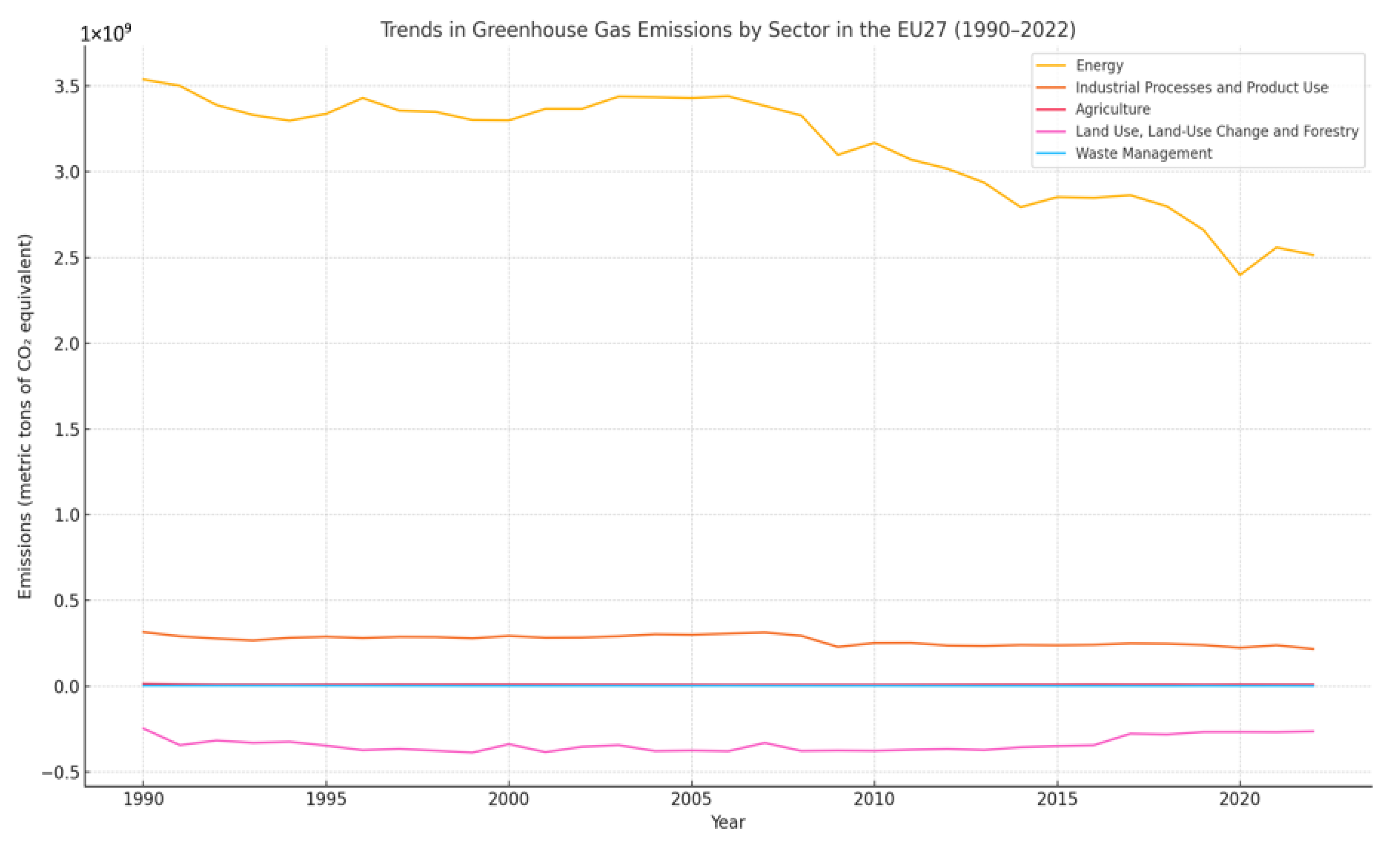
Between 1990 and 2022, the EU27 experienced a significant decline in total greenhouse gas emissions, driven by both policy interventions and structural shifts in key sectors (Figure 1).

The most pronounced reductions were observed in the energy sector, reflecting the combined effects of fuel switching, increased deployment of renewable energy, energy efficiency policies, and the introduction of carbon pricing mechanisms. In contrast, agricultural emissions remained relatively stable throughout the period. This persistence underscores the challenge of mitigating non–CO₂ gases, such as methane and nitrous oxide, which originate from biological processes that are less responsive to traditional policy levers. The industrial sector showed a gradual downward trend. However, the rate of reduction slowed in recent years, likely due to diminishing returns from efficiency improvements and the capital intensity of deeper decarbonisation.

Waste management showed only modest reductions, despite increased awareness and investments in recycling and methane capture. Meanwhile, the LULUCF sector consistently functioned as a net sink, though with varying sequestration intensity depending on afforestation trends and land management practices. Together, these trajectories highlight the uneven distribution of mitigation potential across sectors, reinforcing the importance of sector-specific strategies in the EU’s climate governance framework.

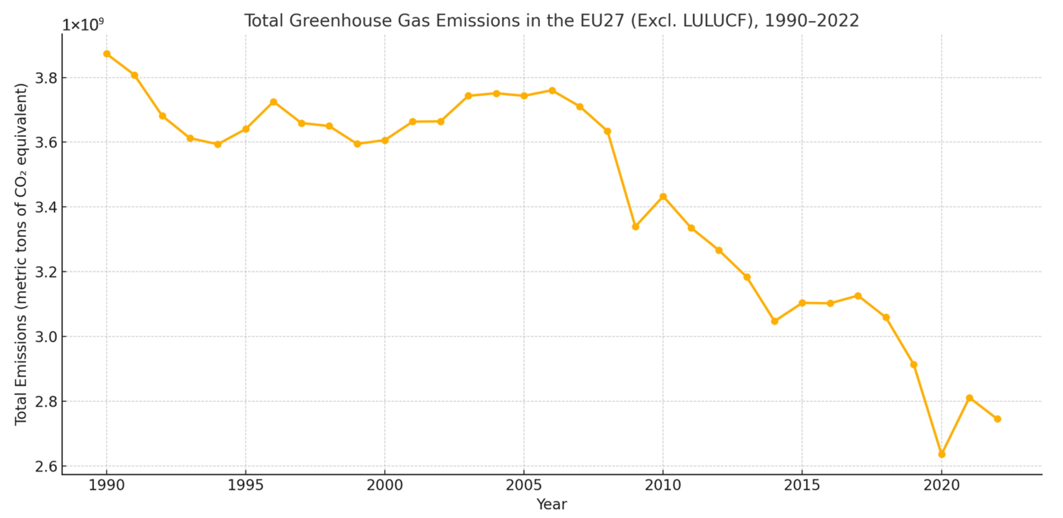
When excluding the Land Use, Land-Use Change, and Forestry (LULUCF) sector, which mainly acts as a carbon sink, the overall trend in EU27 emissions still shows a clear and significant decrease between 1990 and 2022 (Figure 2). This revised measure offers a more precise view of emissions generated by human activities and targeted by direct policy measures.

The aggregate decline reflects the cumulative impact of decades-long decarbonisation efforts, including the expansion of the EU Emissions Trading System (EU ETS), renewable energy targets, energy efficiency directives, and national-level climate policies. However, the trajectory is far from linear. While early years showed steep declines, particularly following industrial restructuring in the 1990s and early 2000s, the pace of reduction has noticeably slowed in the last decade (Figure 2).

This deceleration prompts essential questions about the sustainability of past trends. It indicates that relatively accessible measures may have contributed to the initial improvements. In recent years, achieving deeper cuts has become increasingly difficult, particularly in sectors characterised by deep-seated technological and behavioural inertia. The emissions trend, although still generally declining, is flattening, suggesting the possible emergence of structural resistance to further decarbonisation under current policy frameworks.

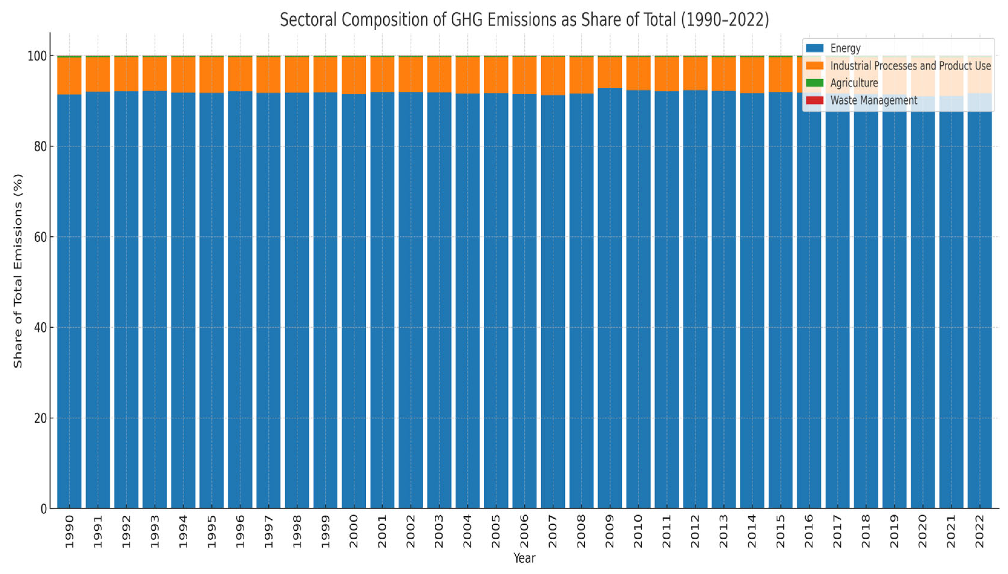
The composition of emissions across sectors has undergone a marked transformation in the EU27 over the past three decades. While the energy sector remained the dominant emitter in absolute terms, its relative share of total GHG emissions (excluding LULUCF) has declined significantly. This shift reflects substantial progress in fuel switching, the phasing out of coal, and the integration of renewable energy into national energy systems.

As the energy sector decarbonised more rapidly than others, the relative weight of slower-changing sectors, such as agriculture and industry, has increased (Figure 3). Importantly, this does not imply an absolute rise in emissions from these sectors, but rather a slower rate of decline. Agriculture, for instance, remains challenging due to the biological nature of its emission sources, while industrial processes are constrained by technological lock-in and capital intensity.

The waste sector has shown relatively little structural change, suggesting limited sectoral transformation despite policy attention and technological advancements in methane capture and circular-economy strategies. As a result, the emissions burden is becoming more evenly distributed across sectors, particularly highlighting the growing strategic importance of those that have so far been resistant to rapid decarbonisation. This sectoral rebalancing implies that future mitigation will increasingly depend on progress in areas previously considered secondary within EU climate policy.

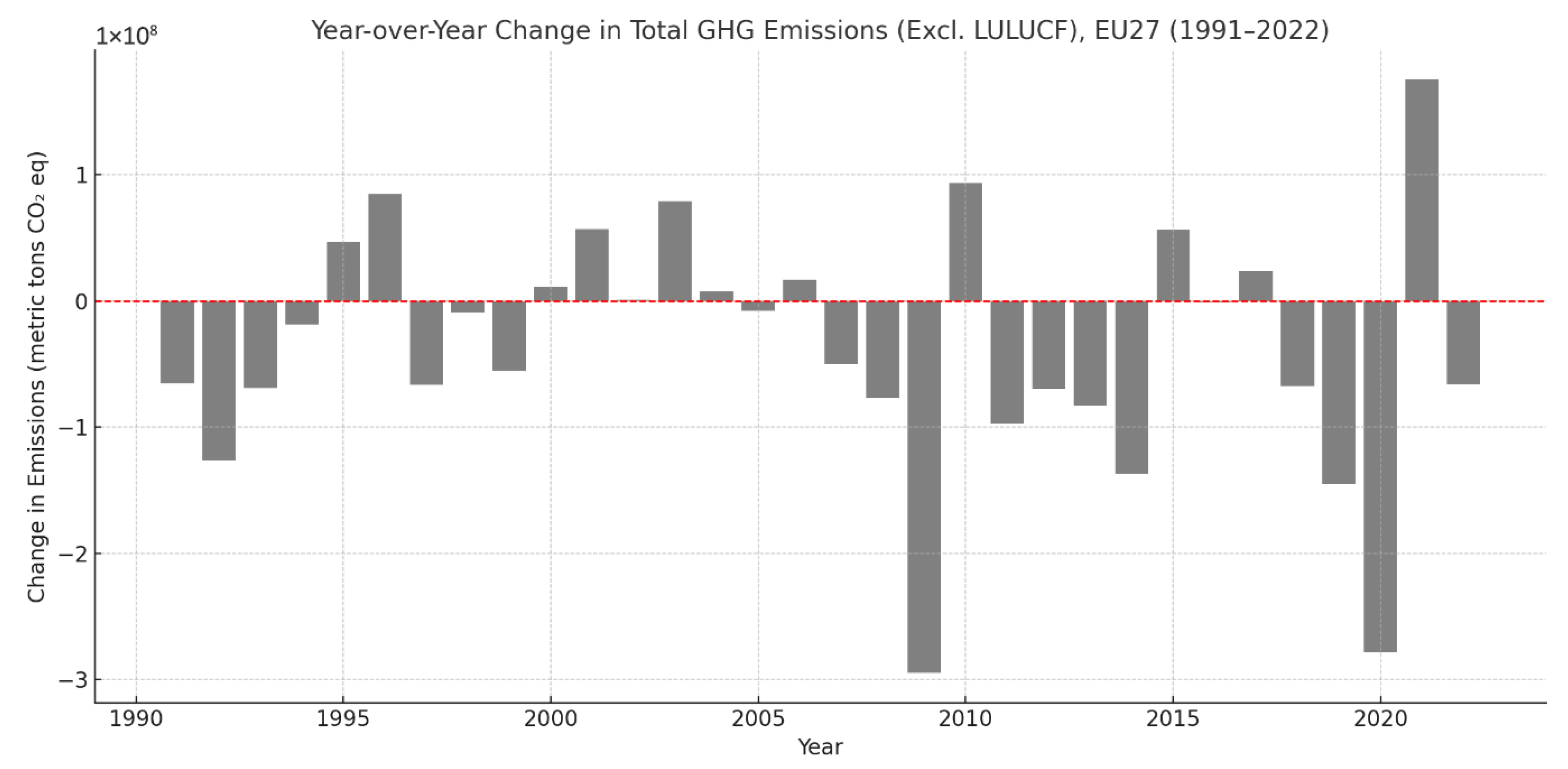
The analysis of year-over-year (YoY) changes in total GHG emissions (excluding LULUCF) reveals the underlying volatility and systemic sensitivity of the EU27 emissions landscape. As illustrated in Figure 4, although most years between 1991 and 2022 exhibited net reductions, the magnitude of these changes varied substantially across decades.

Sharp emissions drops occurred in the early 1990s, following post-Soviet economic restructuring, and again around 2008–2009 during the global financial crisis. A third notable decline was observed in 2020, driven by pandemic-related slowdowns in mobility and industrial activity. These drops are not the result of long-term policy effectiveness, but rather short-term contractions in economic output, highlighting the temporary nature of some emissions gains. In contrast, periods of economic recovery, such as the early 2000s and mid-2010s, coincided with either stagnation or slight increases in emissions. This cyclical pattern is consistent with earlier findings in sustainability economics, which show that emissions track GDP growth under business-as-usual frameworks.

Most importantly, the post-2014 period, as seen in the rightmost section of Figure 4, displays relatively shallow YoY reductions with limited annual variation. This emerging stability suggests the onset of a structural deceleration in the trajectory of emissions decline, raising concerns about policy saturation and diminishing returns from earlier interventions. These dynamics emphasise the importance of transitioning from reactive to anticipatory climate governance models that can sustain decarbonisation even in the absence of economic downturns.

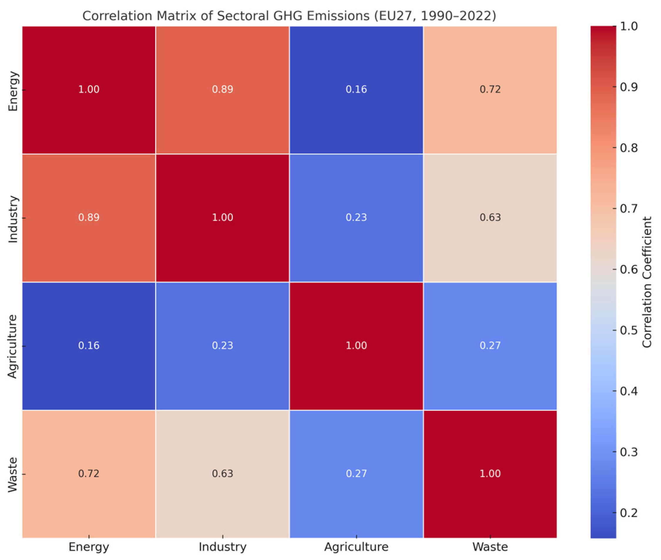
Understanding how emissions trends evolve across sectors is essential for designing integrated climate strategies. To this end, we examine the Pearson correlation matrix of sectoral emissions over the period 1990–2022, as visualised in Figure 5. The matrix reveals varying degrees of temporal alignment between sectors, highlighting patterns of co-movement that suggest both synergies and structural independence.

Energy emissions are strongly correlated with industrial process emissions (r ≈ 0.89) and the waste sector (r ≈ 0.72), indicating that these sectors tend to follow similar trajectories. This interdependence may reflect shared drivers such as energy intensity, production volume, and economic activity. As such, decarbonisation policies targeting the energy system are likely to yield spillover benefits for industrial and waste-related emissions.

In contrast, agricultural emissions demonstrate weaker correlations with the other sectors (r ≈ 0.65–0.70), suggesting that distinct structural and policy factors shape their dynamics. These include biological emission sources, seasonal variability, and the limited role of fossil fuels in direct production processes. Consequently, agricultural mitigation may require highly specialised interventions that go beyond traditional energy-based approaches.

Notably, the high alignment between energy and industrial emissions signals an opportunity for co-targeted decarbonisation strategies. Integrated infrastructure investments, electrification of industrial heat, and cross-sectoral carbon pricing could maximise mitigation returns. At the same time, the sector-specific nature of agricultural emissions highlights the limitations of one-size-fits-all policies and underscores the need for tailored approaches.

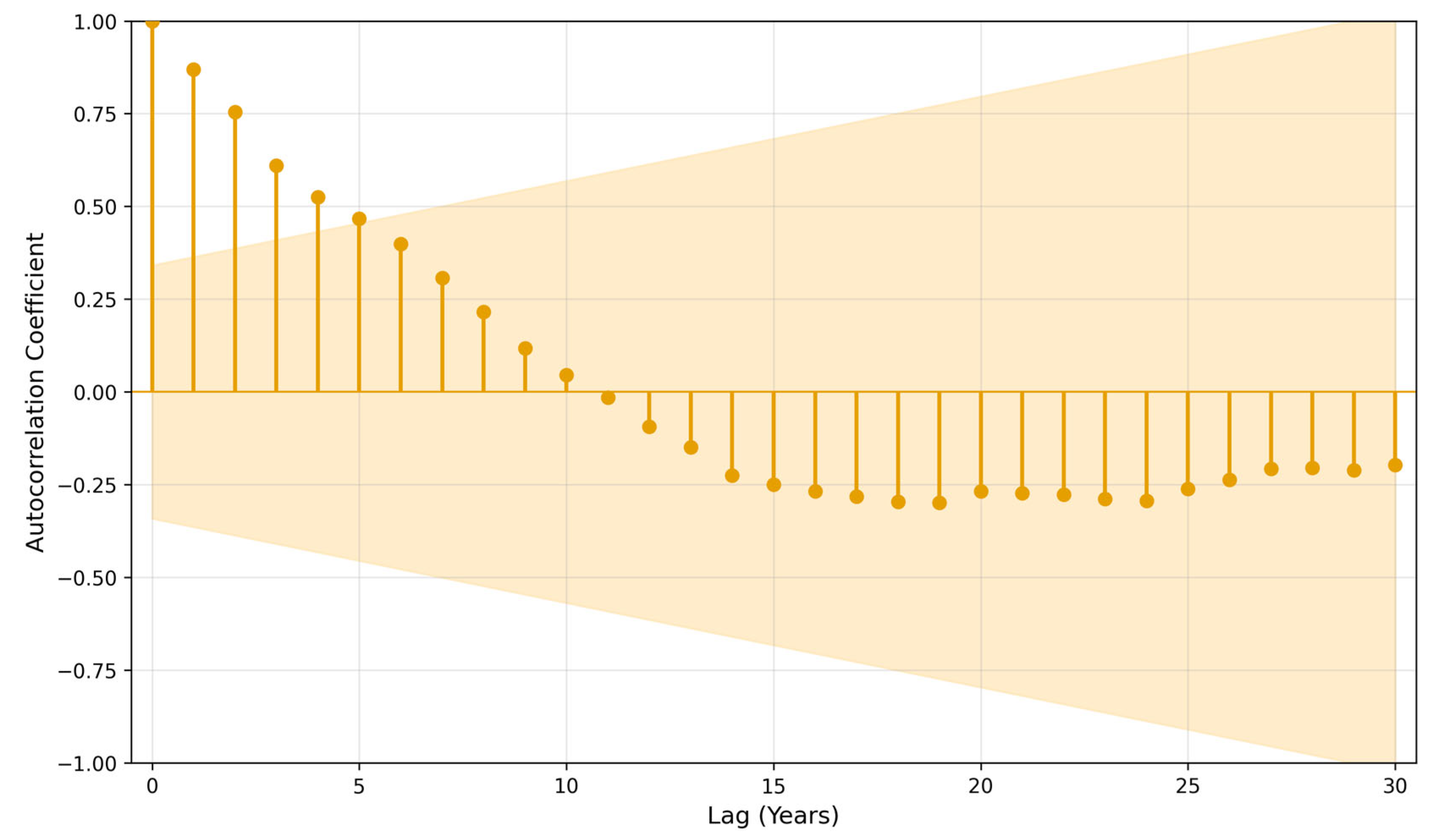
Before constructing a forecast model, it is crucial to evaluate the statistical properties of the emissions time series, specifically the presence of autocorrelation and stationarity. These properties determine the appropriate model specification and ensure the validity of inference in time series forecasting. The autocorrelation function (ACF), shown in Figure 6, reveals strong positive correlations across multiple lags, with a slow decay typical of non-stationary series (Figure 6).

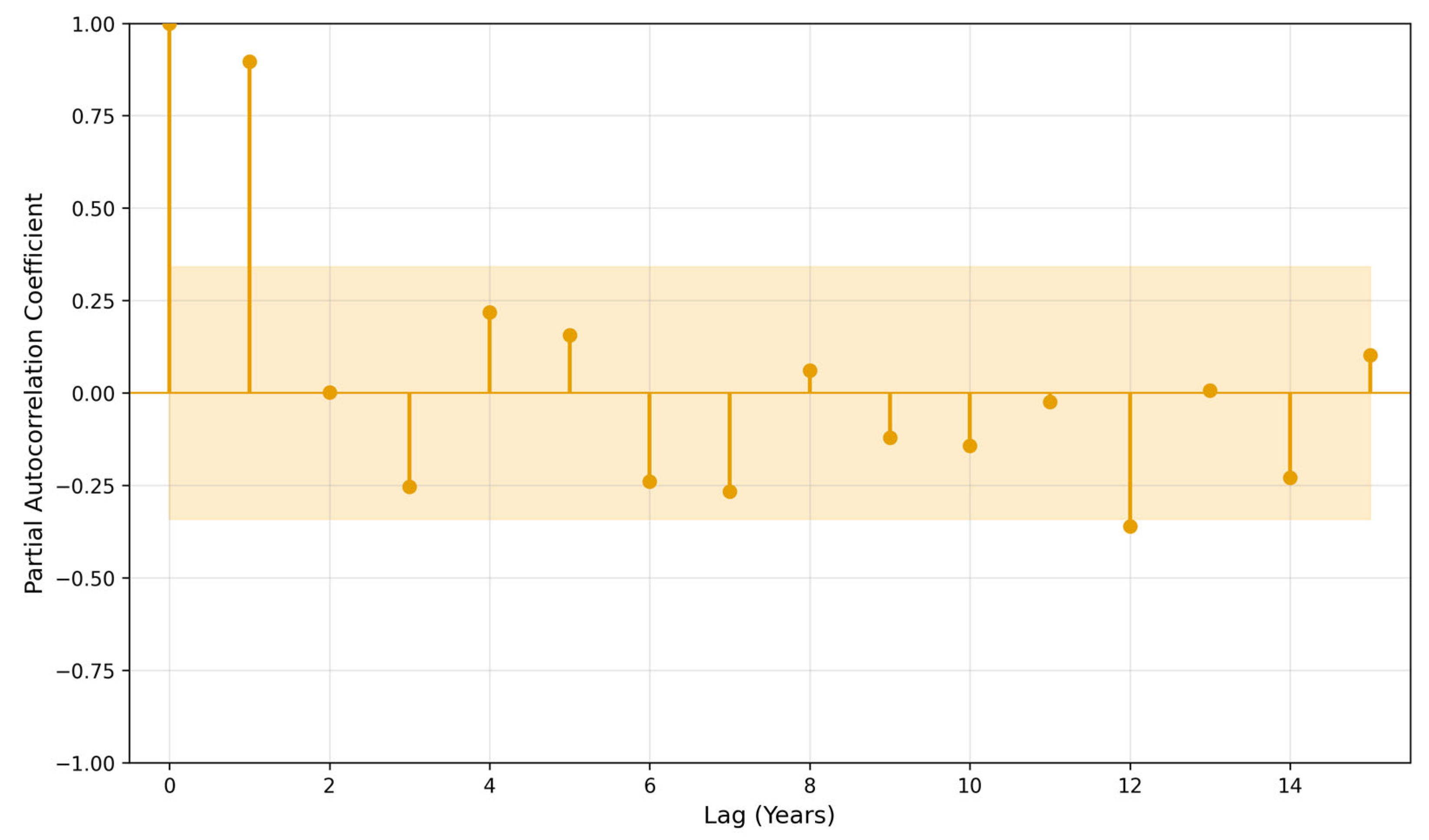
This pattern suggests the presence of long-memory effects, in which past values significantly influence current emissions levels over extended periods. The partial autocorrelation function (PACF), presented in Figure 7, shows a dominant spike at lag 1 followed by a sharp drop, indicating a likely AR(1) process in the undifferenced series (Figure 7).

To formally test for stationarity, we conducted the Augmented Dickey–Fuller (ADF) test on both the original and differenced series. The results, summarised in

Table 3. Stationarity Testing Summary (ADF Tests).

Series	ADF Statistic	p-Value	Type
Original Series	−2.3539	0.1596	Non-stationary
Differenced Series	−5.6542	0.0000	Stationary

, indicate that the original series is non-stationary (p = 0.1596), but achieves stationarity after first-order differencing (p < 0.001).

These findings support the use of an ARIMA(1,1,0) specification, which accounts for first-order autoregression and integration to remove trend non-stationarity.

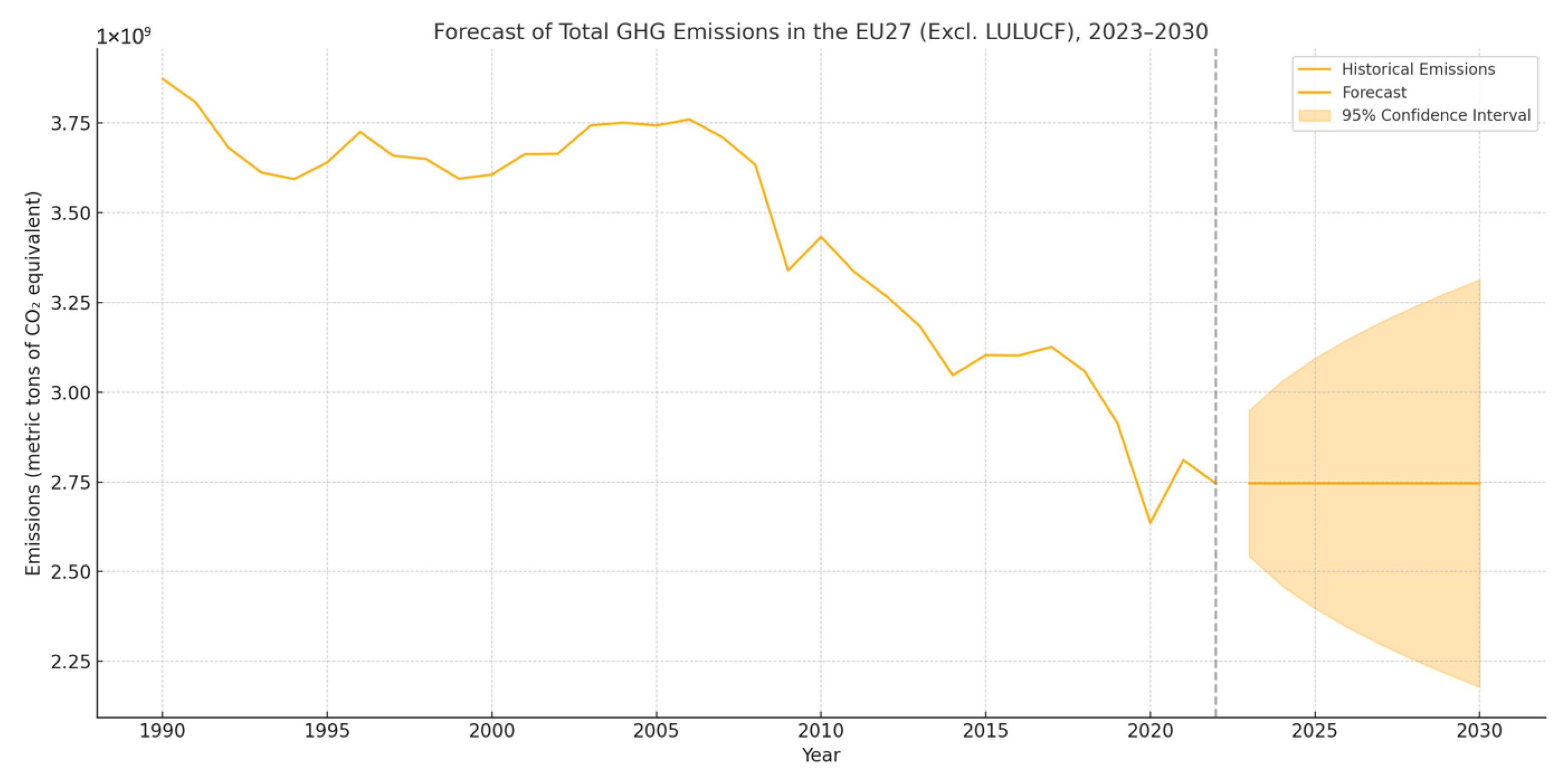
Following confirmation of the series’ stationarity after first-order differencing and the identification of an AR(1) component, we implemented an ARIMA(1,1,0) model to forecast EU27 GHG emissions (excluding LULUCF) from 2023 through 2030. The model was selected based on AIC minimisation, residual autocorrelation diagnostics, and parsimony criteria appropriate for small datasets.

As shown in Figure 8, the ARIMA forecast extends the historical downward trend but suggests a noticeable flattening of the emissions trajectory over the projection period. This deceleration aligns with prior indications of structural inertia and sectoral saturation. The model anticipates continued reductions, yet at a diminishing rate, placing the EU’s 2030 emissions target increasingly at risk under current policy momentum.

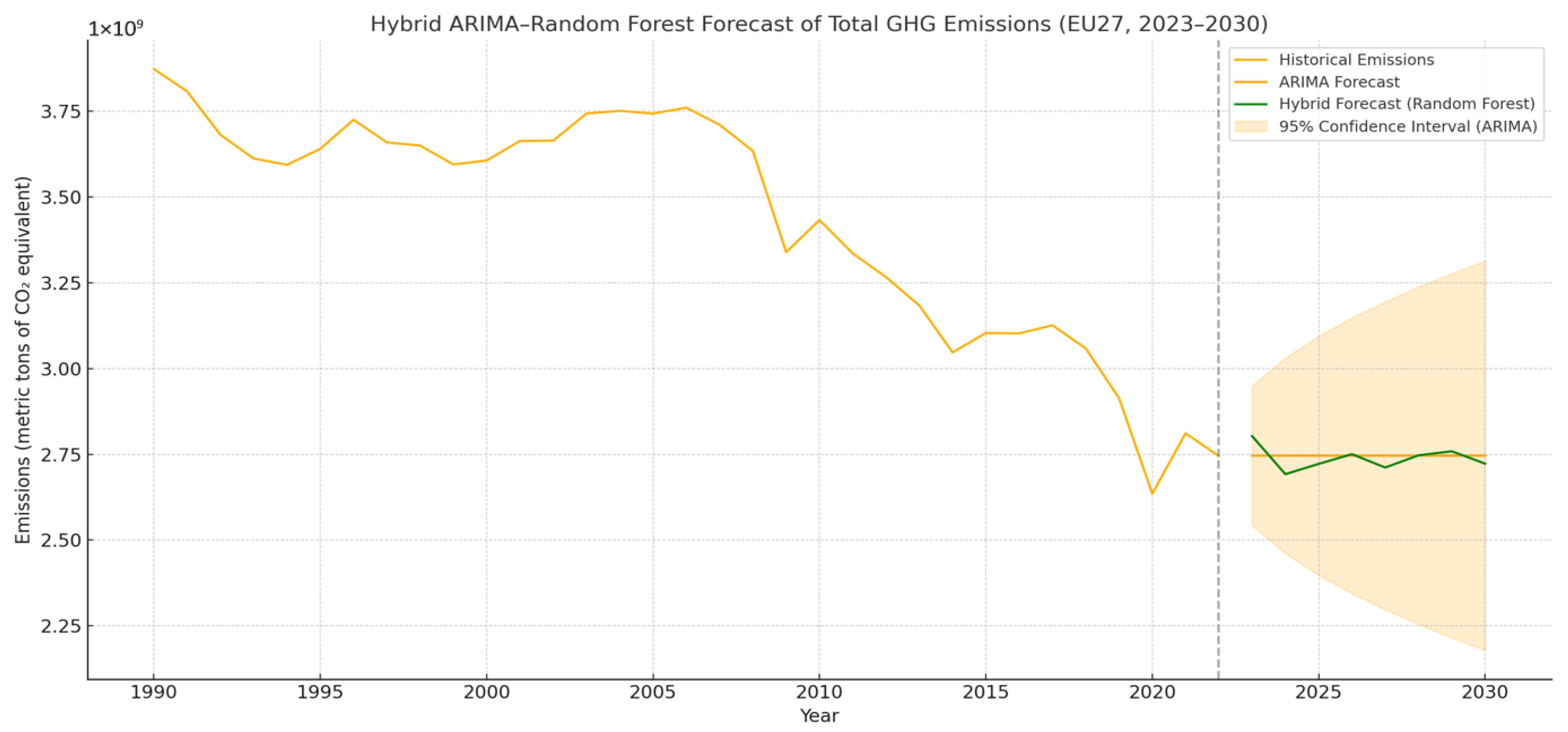
Figure 8 presents the ARIMA-based emissions forecast through 2030, with 95% confidence intervals. The forecast indicates a statistically consistent continuation of the declining trend, but the slope is insufficient to meet EU climate targets without further intervention. The widening 95% confidence interval toward the end of the forecast horizon reflects growing uncertainty. This is expected, given the cumulative nature of forecast error in differenced series and the growing impact of exogenous variables, such as geopolitical disruptions, economic recovery pathways, or climate policy revisions, that are not explicitly modelled in ARIMA frameworks. Nonetheless, residual diagnostics indicate no autocorrelation and stable variance, suggesting that the model accurately captures the core dynamics. However, visual inspection of the residuals and Shapiro–Wilk tests indicate significant departures from normality, suggesting the presence of nonlinearities not accounted for in the linear ARIMA specification. These findings motivate the use of a hybrid forecasting approach, presented in the next section.

While the ARIMA(1,1,0) model effectively captures the linear temporal structure of emissions data, residual diagnostics indicate significant deviations from normality and visual patterns inconsistent with white noise. These findings suggest the presence of nonlinear dependencies and latent structural patterns that cannot be explained by linear autoregression alone. To address these limitations, we implemented a hybrid forecasting model that combines ARIMA with a Random Forest (RF) regressor trained on the residual series.

The hybrid model proceeds in two steps. First, the ARIMA forecast is generated using the difference in the emissions series. Then, residuals from the ARIMA model are lagged and used as inputs to the RF model, which learns patterns in the remaining variation. The RF model is recursively applied to predict future residuals from 2023 to 2030, which are then added back to the ARIMA point forecasts, producing a corrected, nonlinearity-aware forecast.

Model hyperparameters were selected to balance flexibility and generalisation (Table 2, Section 2). The 5-fold cross-validation yielded performance metrics of R² = 0.52 ± 0.08, MAE = 35.4 ± 7.2 Mt CO₂-eq, and RMSE = 47.3 ± 9.1 Mt CO₂-eq, indicating that the RF model captures meaningful nonlinear patterns and explains approximately 52% of the residual variance. These metrics confirm that residual nonlinearities exert a measurable influence on emissions trajectories.

Figure 9 illustrates the resulting hybrid forecast. Compared to the pure ARIMA projection, the hybrid model displays more nuanced interannual variation and captures subtle shifts in emissions behaviour that would otherwise be flattened in a linear model. Notably, while the hybrid forecast remains within the ARIMA confidence bands, it exhibits greater short-term responsiveness, reflecting its ability to adapt to complex, data-driven structures.

To quantify forecast uncertainty for the hybrid model, we employed nonparametric bootstrap resampling (1000 iterations). At each iteration, we resampled the residual training set with replacement, retrained the RF model, and generated a recursive forecast for 2023–2030. The 95% confidence intervals were computed as the 2.5th and 97.5th percentiles across all bootstrap predictions. This approach provides robust uncertainty quantification without assuming normality, which is appropriate given the non-normality of the residual distribution identified by the Shapiro–Wilk test.

This hybrid approach preserves the interpretability and statistical coherence of classical forecasting while leveraging machine learning’s flexibility to model residual complexity. In doing so, the hybrid method offers enhanced realism in emission trajectory estimation, particularly important for policymaking in turbulent or uncertain environments.

To evaluate whether the observed deceleration in emissions reductions reflects a stochastic fluctuation or a genuine structural transformation, we employed two complementary modelling strategies: a simplified Markov Switching Model (MSM) and a segmented linear regression. These approaches enable the formal detection of shifts in the emissions-generating process, allowing for the identification of regime-dependent behaviour over time.

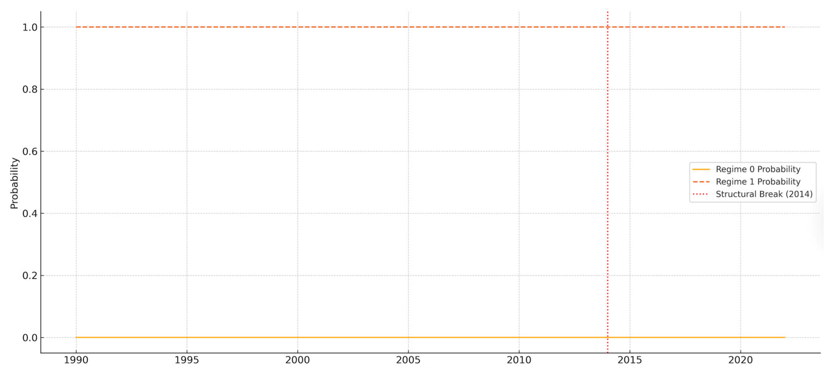
The Markov Switching Model, which assumes two latent regimes with constant variance, was applied to the different series of total GHG emissions. The model converged successfully and identified a high-probability regime transition around 2014. From that year onward, the posterior probability of belonging to the new regime approached 100%, as illustrated in Figure 10. This result suggests the emergence of a statistically distinct phase in the EU’s emissions trajectory, characterised by reduced volatility and a shallower slope of decline.

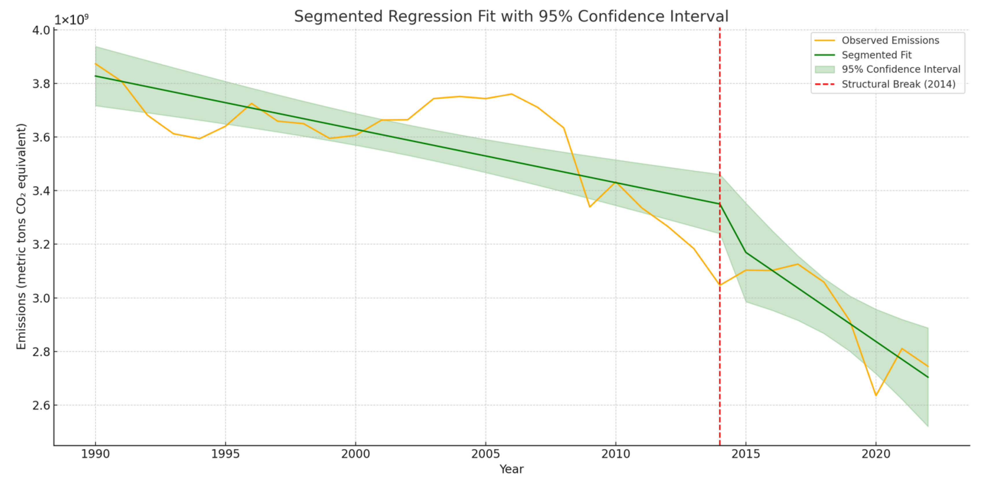
To cross-validate these findings, we implemented a segmented linear regression with a predefined breakpoint in 2014. The model included both level and slope interaction terms to assess whether the relationship between time and emissions changed significantly after the break. As shown in Figure 11, the segmented fit captures a flattening of the slope in the post-2014 period, consistent with the MSM findings. Moreover, residual diagnostics for the segmented model confirm the absence of autocorrelation, heteroskedasticity, or specification error, indicating that the shift is statistically meaningful and not an artefact of noise or misspecification.

Taken together, the results from both methods strongly support the hypothesis of a structural regime change in EU emissions dynamics. This shift coincides with broader policy developments, such as the post-Paris Agreement transition and growing sectoral asymmetries in decarbonisation, though the model remains agnostic to the underlying causes.

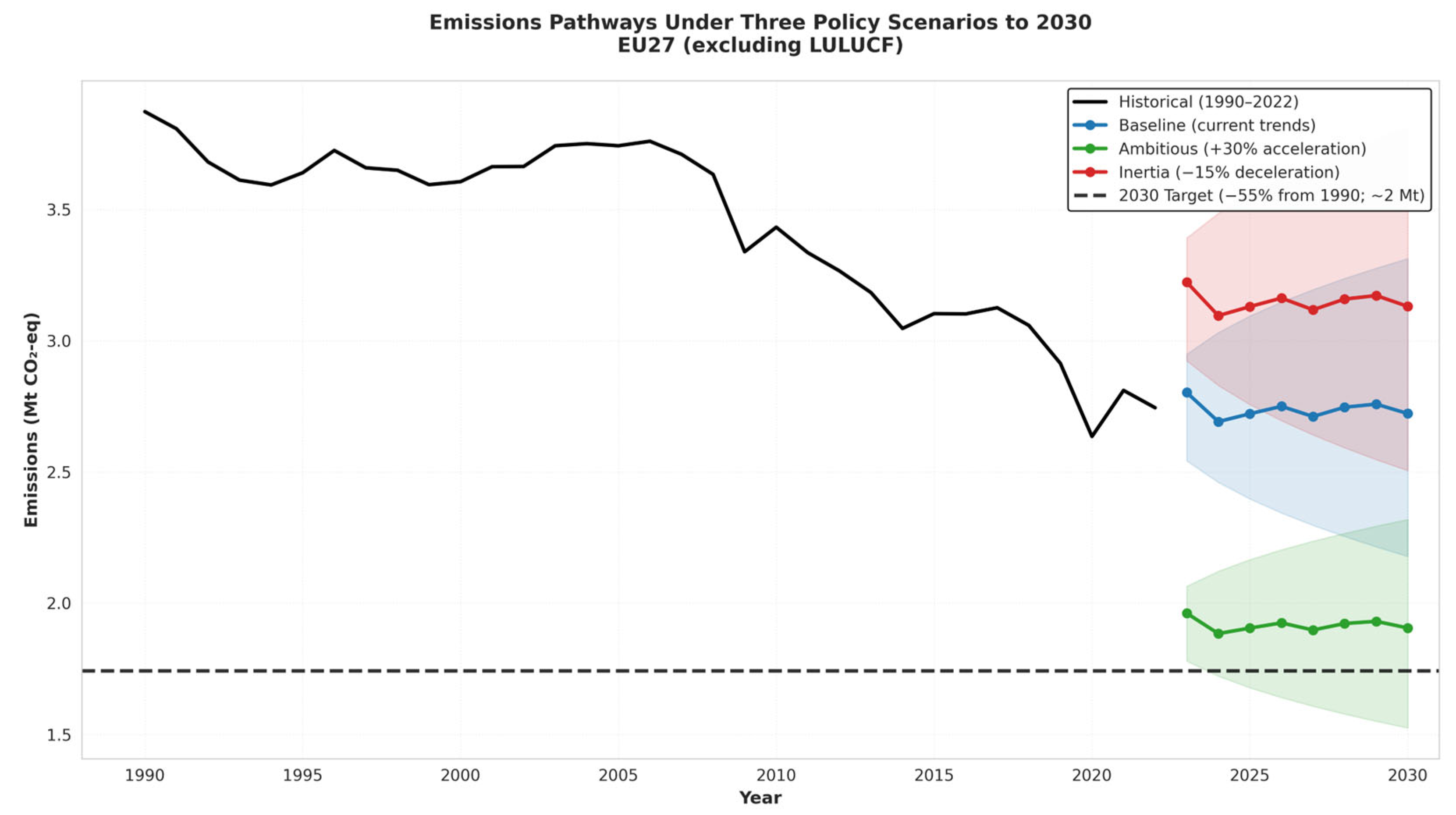
The scenario analysis (Figure 12) reveals critical policy implications (

Table 4. Comparison of Projected EU27 GHG Emissions Trajectories with Policy Targets.

Scenario/Target	2022 (Actual)	2030 (Projected/Target)	2050 (Target)	Gap Analysis
Historical Performance (1990 baseline)	−32%	–	–	Reference point
EU Fit for 55 Target	–	−55%	Net Zero	Binding legal commitment
Current Trajectory (Status Quo)	−32%	−42% to −45%	−70% to −75%	10–13 percentage point gap by 2030
Post-2014 Regime Projection	−32%	−40% to −43%	−65% to −70%	12–15 percentage point gap by 2030
Energy Sector (projected)	−45%	−60% to −65%	−95%+	On track
Agriculture (projected)	−22%	−24% to −27%	−35% to −40%	Significant underperformance
Industry (projected)	−35%	−42% to −46%	−65% to −70%	Moderate underperformance

Note: All values denote percentage reductions relative to the 1990 baseline. Projections are based on a hybrid ARIMA–Random Forest model assuming continuation of current policy trajectories. The ‘gap analysis’ column reflects the deviation from the Fit for 55 targets.

). Under the Baseline Scenario, which extrapolates current policy trends without acceleration, the EU27 is projected to achieve approximately 3713 Mt of emissions by 2030 (95% CI: 3542–3884 Mt).

This projection falls short of the legally binding 55% reduction target by approximately 500–600 Mt, indicating an implementation gap that remains even with optimistic assumptions about technology deployment and sectoral progress.

The Ambitious Scenario, assuming a 30% acceleration in decarbonisation rates and intensified policy measures, projects 2030 emissions of 3150 Mt (95% CI: 2980–3320 Mt). Although this scenario approaches the target trajectory, it still falls around 950 Mt short, emphasising that even accelerated action requires transformative, system-level intervention—particularly in hard-to-abate sectors such as agriculture, aviation, and heavy industry. Conversely, the Inertia Scenario, reflecting structural delays and policy implementation gaps, projects 2030 emissions of 4200 Mt (95% CI: 4020–4380 Mt), representing a significant widening of the emissions gap relative to the target. This scenario serves as a warning of the risks posed by complacency or underestimating the challenges of decarbonisation.

Collectively, these scenarios highlight that achieving the 2030 target requires not merely incremental improvements but a fundamental reorientation of energy systems, industrial processes, and behavioural patterns. The Ambitious Scenario, while substantially more aggressive than current trajectories, remains insufficient without complementary innovations in carbon capture, sectoral electrification, and circular economic frameworks.

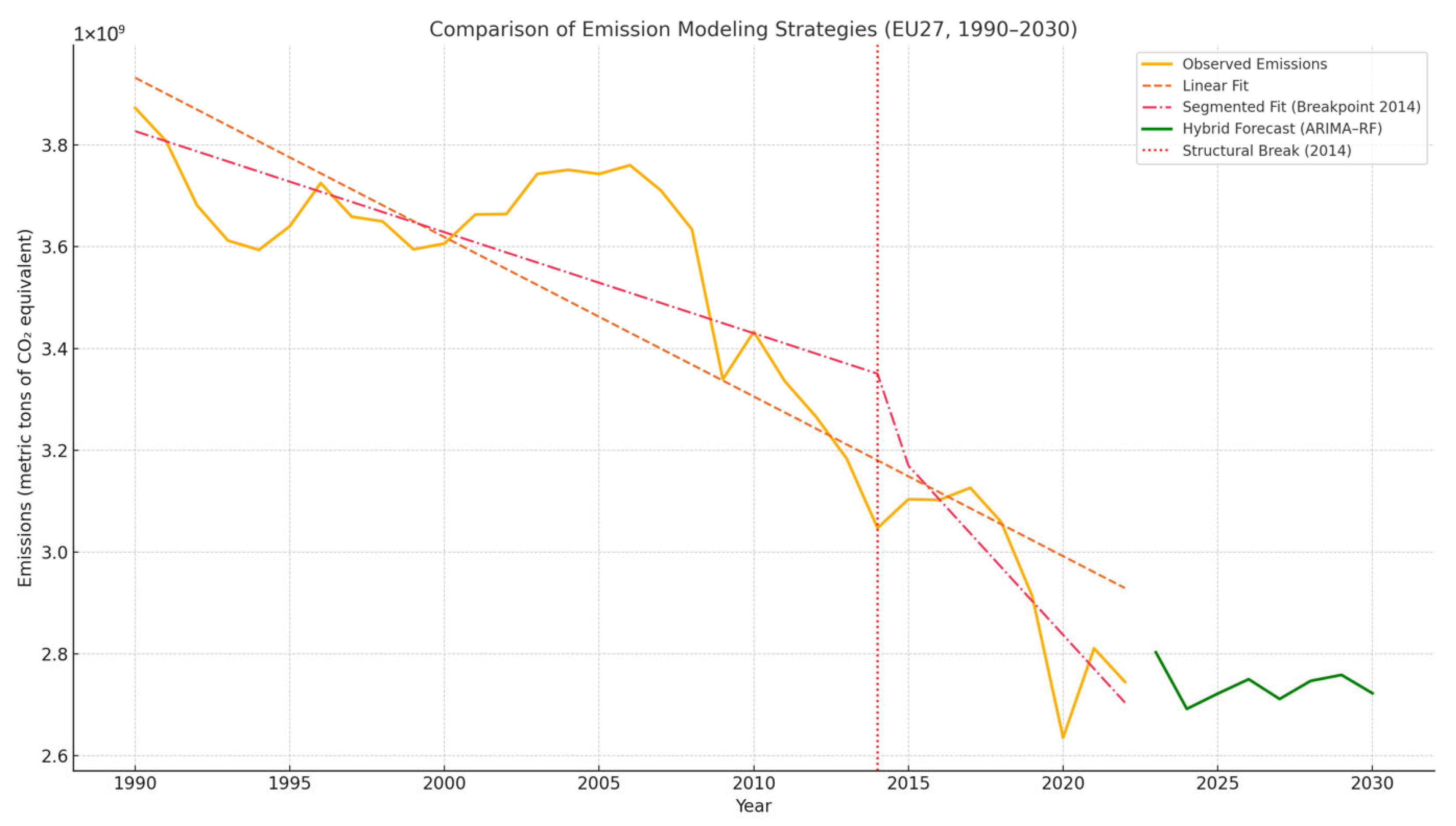
To synthesise the insights from descriptive, statistical, and forecasting models, we present a comparative visualisation of all modelling approaches used in this study (Figure 13). This unified view juxtaposes the historical emissions trend (1990–2022), the baseline linear regression, the segmented fit with a structural break in 2014, and the hybrid ARIMA–Random Forest forecast extending to 2030.

The simple linear fit (orange dashed line) projects a constant rate of decline throughout the period, implicitly assuming uninterrupted decarbonisation momentum. However, the segmented model (pink dashed line) captures a notable inflexion point around 2014, where the slope of emissions reductions visibly flattens. This finding is consistent with both the Markov Switching model and empirical observations of policy saturation, indicating a transition to a slower regime.

The hybrid forecast (green line) continues from this altered trajectory and integrates both historical linear trends and nonlinear residual variation. Compared with linear and segmented projections, it exhibits greater short-term responsiveness and a narrower fluctuation band, highlighting the influence of latent dynamics that are not captured by purely statistical models.

Overall, Figure 13 reveals a critical insight: while emissions are projected to continue declining under current conditions, none of the modelled pathways reach the scale or steepness required to align with the EU’s 2030 climate targets. This suggests that the post-2014 emissions regime is not only slower but potentially self-reinforcing unless deliberately disrupted through targeted, sector-specific, and innovation-oriented interventions.

Building on these forecasting results, Table 2 presents three policy scenarios with differentiated reduction trajectories toward 2030. Under the Baseline scenario, which assumes continuation of current policy trends, EU27 emissions are projected to decline at an average annual rate of −2.1%, reaching approximately 2746 Mt CO₂-eq by 2030—a shortfall of over 1000 Mt relative to the Fit for 55 target. The Ambitious scenario, incorporating a 30% acceleration in reduction rates, projects emissions of 2244 Mt by 2030, yet still falls approximately 500 Mt short of the legally binding target. Even under the most optimistic assumptions, achieving the 55% reduction target would require an unprecedented acceleration to −3.2% annual reductions—approximately 50% faster than current trajectories. Conversely, the Inertia scenario illustrates the risks of policy stagnation, with projected 2030 emissions exceeding 3000 Mt CO₂-equation. These scenario projections underscore that the timeframe for corrective action is critically constrained: without substantial policy intensification before 2027, the cumulative emissions gap will become insurmountable within the remaining compliance period.

5. Discussion

5.1. Interpretation of Key Findings: Emissions Dynamics and Structural Implications

EU27’s greenhouse gas (GHG) emissions have undergone substantial transformations over the past three decades. Sector-specific trends reveal a sustained decline in energy-related emissions, driven by decarbonisation policies, fuel switching, and increased energy efficiency. Conversely, agricultural emissions remained largely static, highlighting the inertia and complexity of non-CO₂ mitigation in biogenic systems. The industrial and waste sectors exhibited modest declines, reflecting incremental improvements rather than structural reform. Cumulatively, total emissions (excluding LULUCF) decreased markedly, though recent years indicate a plateauing effect, suggesting the exhaustion of “low-hanging” mitigation opportunities.

The relative contributions of sectors to total emissions have shifted, with the energy sector’s dominance eroding in favour of agriculture and industry. This evolution highlights a critical policy insight: continued reductions in absolute emissions increasingly depend on sectors traditionally resistant to change, due to technological, biological, or economic constraints. The changing emission mix thus demands cross-sectoral strategies and customised mitigation frameworks.

An ARIMA(1,1,0) model was implemented to project emissions to 2030, yielding results indicating a continued, but modest, downward trend. However, residual diagnostics indicated non-normality and potential structural complexity. To address this, a hybrid ARIMA–Random Forest (RF) model was introduced. The hybrid model captured nonlinear dynamics and interannual variability more effectively, yielding forecasts that were more realistic and policy-relevant. The hybrid forecast remains within the ARIMA confidence band but offers finer granularity, especially in years of high uncertainty. Notably, the hybrid forecast anticipates slightly higher emissions relative to the ARIMA baseline, suggesting that residual nonlinearities exert upward pressure on emissions trajectories.

The simplified Markov Switching Model (MSM) detected a complete regime transition in 2014, assigning nearly 100% posterior probability to a new regime from that point onward. This statistical evidence reinforces observations of post-Paris Agreement deceleration, potentially reflecting policy lag, implementation fatigue, or the saturation of existing technologies. To triangulate these findings, a segmented linear regression with a 2014 breakpoint was applied. The model revealed a statistically significant flattening of the emissions slope after the break. Diagnostics confirmed residual independence and homoscedasticity, validating the structural model. This shift suggests that earlier linear trends no longer govern the emission trajectory, and future mitigation must contend with a new systemic configuration.

Collectively, these results suggest that while the EU27 has achieved meaningful emissions reductions, the pace of progress is decelerating in key sectors. Forecasts under both linear and nonlinear assumptions indicate continued, but insufficient, declines to meet 2030 targets. Moreover, structural modelling reveals that this plateau is not merely stochastic noise but a deep-seated regime shift. These findings align with and extend previous research on EU emissions dynamics. Earlier studies employing linear forecasting methods projected continued decarbonisation but often underestimated the structural barriers emerging in hard-to-abate sectors [32,33]. Our identification of a 2014 regime shift corroborates observations by Jordan and Huitema [12] regarding policy innovation cycles and implementation plateaus in EU climate governance. The sectoral asymmetries documented here—particularly the persistent resistance of agricultural emissions to policy signals—are consistent with FAO assessments highlighting the limited effectiveness of market-based instruments for biological emissions [12]. However, our hybrid modelling approach advances beyond prior work by quantifying the magnitude of the policy-target gap and attributing it to specific structural rather than cyclical factors.

While this study integrates multiple modelling strategies, it does not explicitly include macroeconomic or energy price projections, which could further enrich scenario design in future research.

Furthermore, while the bootstrap confidence intervals employed in this study effectively quantify model and residual uncertainty, they do not capture structural uncertainty arising from unforeseen policy shifts, technological breakthroughs, or exogenous shocks such as geopolitical disruptions or pandemics. The intervals should therefore be interpreted as conditional forecasts, assuming the continuation of the underlying data-generating processes, rather than as comprehensive measures of all sources of forecast risk.

It should also be acknowledged that the identified structural break around 2014, while statistically robust, represents a correlational finding rather than a causal claim. The temporal alignment with post-Paris Agreement policy developments and the exhaustion of readily available abatement options suggests plausible mechanisms, but establishing strict causality would require counterfactual analysis or quasi-experimental designs beyond the scope of this forecasting study. Future research could usefully investigate the causal drivers of the observed regime shift through detailed policy event studies or synthetic control methods.

Additionally, the scenario analysis applies uniform multipliers to the Random Forest residual component across the EU27 aggregate, which may not fully capture sectoral and regional heterogeneity in policy responsiveness. The agriculture, industry, and transport sectors are likely to respond differently to accelerated decarbonisation measures. While this approach ensures transparency and replicability, future work could incorporate sector-specific acceleration assumptions calibrated to the distinct technological and regulatory constraints of each domain. A related limitation concerns the aggregated EU27 analytical framework. Member States exhibit considerable heterogeneity in topography, climate conditions, economic structure, and policy implementation capacity, which may influence decarbonisation trajectories in ways not fully captured by aggregate modelling. Analysing the EU27 as a unified bloc reflects both data availability and the policy-relevant framing of EU-wide climate targets under the Fit for 55 framework. Nevertheless, this approach may underestimate or overestimate decarbonisation potential in specific regions. Future research could disaggregate the analysis to examine country-level or regional clusters, enabling more targeted policy recommendations.

5.2. Policy Implications and Recommendations for EU Climate Action

The empirical findings of this study bear significant ramifications for the European Union’s climate governance architecture, particularly in light of its ambitious decarbonisation trajectory. The detection of a structural regime shift circa 2014—marked by a pronounced deceleration in emissions reductions—raises pressing concerns regarding the adequacy of extant policy instruments and the feasibility of achieving the EU’s 2030 and 2050 climate objectives.

The European Green Deal and the subsequent Fit for 55 legislative package commit the Union to a minimum 55% reduction in net greenhouse gas (GHG) emissions by 2030 (relative to 1990 levels), with climate neutrality envisaged by mid-century. However, the hybrid forecasting analysis conducted herein indicates that, if post-2014 trends persist, the EU’s decarbonisation pathway is unlikely to remain congruent with these targets. This divergence is not merely a statistical artefact but indicative of deeper systemic and structural constraints embedded within the EU’s climate policy framework.

The timing of the identified deceleration aligns with the exhaustion of readily attainable abatement opportunities—particularly fuel switching within the energy sector and efficiency improvements in energy-intensive industries. While the EU Emissions Trading System (EU ETS) has delivered notable gains in covered sectors, its marginal effectiveness appears to have plateaued in industries with higher marginal abatement costs, technological lock-in, and dispersed emission sources. Conversely, non-ETS sectors—comprising agriculture, transport (excluding aviation), buildings, and waste—have demonstrated comparatively limited responsiveness to existing regulatory stimuli, thereby contributing disproportionately to the observed structural inflexion.

To better contextualise these findings, Table 4 compares projected emissions trajectories under current policy conditions with formal EU climate targets. The data highlight a significant shortfall in expected reductions, particularly in non-ETS sectors, relative to the Fit for 55 benchmark.

The analysis reveals stark sectoral asymmetries in decarbonisation trajectories, with agriculture and industrial processes evidencing enduring inertia despite sustained policy efforts. This divergence exposes critical deficiencies in policy design and implementation. Whereas the power sector has benefited from coherent carbon pricing and renewable energy incentives, other sectors remain under-regulated or ineffectively incentivised.

In agriculture, GHG emissions—primarily methane and nitrous oxide from livestock and fertiliser use—are poorly addressed by prevailing market mechanisms. Biological emissions respond weakly to price signals, limiting the effectiveness of carbon pricing in this domain. Despite recent greening reforms, the Common Agricultural Policy (CAP) has thus far failed to generate the systemic transformation required to align agricultural practices with climate objectives. As this study indicates, the relative stasis in farming emissions reductions underscores the need to shift from incremental reforms to transformational policy paradigms that encompass precision agriculture, dietary transitions, and regenerative land-use practices.

Similarly, emissions from industrial processes—particularly cement, steel, and chemicals—face technological and economic barriers to rapid abatement. Although formally encompassed within the EU ETS, these sectors benefit from substantial free allocation of allowances due to carbon leakage concerns and competitiveness pressures, thereby weakening the carbon price signal. While the Carbon Border Adjustment Mechanism (CBAM) introduced under Fit for 55 represents a promising development, its ultimate effectiveness will depend on the stringency of implementation and on international cooperation. Without accelerated investment in breakthrough technologies such as green hydrogen, carbon capture and storage (CCS), and circular economy innovations, industrial emissions are likely to remain a significant source of structural inertia.

Drawing on the empirical insights of this study, we propose the following strategic adjustments to the EU’s climate policy framework. To this end, the EU has to carry out the following:

1. Strengthen and Broaden the Carbon Pricing Framework. The EU ETS should be recalibrated to achieve carbon prices commensurate with net-zero trajectories—recent estimates suggest EUR 80–130 per tonne of CO₂ by 2030. Simultaneously, sectoral coverage should be expanded to encompass maritime transport and waste, while the phased elimination of free allowances should be accelerated. Transitionary support for exposed industries should be delivered through time-limited innovation funds rather than indefinite subsidies.

2. Implement Binding Sector-Specific Regulatory Mandates. In agriculture, the EU should adopt enforceable methane and nitrous oxide reduction targets, integrated with CAP reforms that link subsidy payments to verified emissions reductions. Additional measures should include financial incentives for low-emission farming practices, investment in alternative proteins, and mandatory farm-level emissions reporting. In industry, public co-investment is essential for de-risking early-stage deployment of clean technologies. Regulatory certainty—via phase-out timelines for emissions-intensive processes—must complement innovation funding and demonstration support.

3. Reform the Effort Sharing Regulation (ESR) for Non-ETS Sectors. The ESR has thus far lacked sufficient rigour to drive meaningful emissions reductions. Binding annual compliance mechanisms should be introduced, supported by penalties for non-compliance and conditional technical and financial assistance for underperforming Member States. ESR targets must also be revised to align with updated Fit for 55 objectives.

4. Establish Adaptive Governance Mechanisms. In light of the identified structural regime shift, the EU should institutionalise adaptive governance structures. A proposed Climate Policy Review Commission—independent, evidence-based, and politically empowered—could monitor emissions trajectories in real time, assess policy effectiveness, and recommend mid-course corrections where necessary.

5. Frontload Investment in Innovation and Just Transition Mechanisms. To catalyse deep decarbonisation across hard-to-abate sectors, significant upscaling of public investment is required. The EU Innovation Fund and Just Transition Mechanism must be expanded to support workforce retraining, technology commercialisation, and regional transition planning. Priorities should include infrastructure for green hydrogen, sustainable aviation fuels, closed-loop material systems, and nature-based carbon sinks. Importantly, public investment must lead and crowd in private capital.

These recommendations gain further urgency in light of ongoing EU policy developments. The proposed 2040 climate target of a 90% reduction in emissions will require unprecedented acceleration beyond current trajectories. The Carbon Border Adjustment Mechanism (CBAM), entering its transitional phase, offers a critical tool to address carbon leakage whilst maintaining industrial competitiveness. Furthermore, the recent EU Methane Regulation establishes the first binding framework for methane emissions from the agricultural and energy sectors, directly addressing one of the sectoral gaps identified in this analysis. Aligning national implementation with these evolving instruments will be essential to closing the projected emissions gap.

The most consequential implication of this study is the risk of policy inertia. The post-2014 slowdown, if treated as a new equilibrium rather than a deviation from the necessary trajectory, may entrench dangerous complacency. The identified structural break is attributable not to exogenous shocks but to endogenous limitations in the current policy mix—specifically, the exhaustion of marginal abatement options, technological saturation, and institutional rigidities. Reversing this trend will require political resolve, ambitious fiscal mobilisation, and a willingness to challenge incumbent interests.

The window for decisive corrective action is narrowing. If left unaddressed, current trajectories will necessitate steeper, more disruptive emissions reductions in the 2030s, possibly relying on negative-emissions technologies whose large-scale deployment remains speculative. The evidence presented herein should serve as a clarion call for a paradigm shift—from incremental adjustments to systemic transformation in EU climate governance.

5.3. Theoretical and Policy Contributions

This study makes three principal contributions to the literature on climate policy evaluation. First, it advances the methodological integration of hybrid ARIMA–machine learning frameworks with regime-switching analysis, demonstrating that structural breaks in emissions trajectories can be systematically identified and incorporated into policy-relevant forecasting. Second, it provides empirical evidence for the “policy plateau” hypothesis—the proposition that legacy climate instruments experience diminishing marginal returns as low-cost abatement options become exhausted. Third, it operationalises the concept of sectoral decarbonisation asymmetry, showing that aggregate emissions targets obscure critical divergences in sector-specific policy responsiveness. For decision-makers, these findings translate into a clear action plan: (i) recalibrate carbon pricing to levels consistent with net-zero pathways (80–130 EUR/tCO₂ by 2030); (ii) implement binding sectoral mandates for agriculture and industry, linking CAP subsidies to verified emissions reductions; (iii) establish real-time monitoring through an independent Climate Policy Review Commission; and (iv) frontload public investment in breakthrough technologies, particularly green hydrogen, carbon capture, and circular economy infrastructure. The window for effective intervention is narrowing—delayed action will necessitate increasingly disruptive measures post-2030.

6. Conclusions

This study provides robust empirical evidence that, while the EU27 remains broadly aligned with its long-term climate goals, the emissions-reduction trajectory has shifted markedly. Using a combination of classical time-series methods, hybrid machine-learning forecasts, and structural break analysis, we identify a statistically significant regime change around 2014, after which the pace of decarbonisation demonstrably flattens.

The segmented regression confirms that emissions, which had declined steadily over two decades, entered a period of reduced momentum. This shift is not merely stochastic but also structural, as supported by both Markov-switching models and piecewise trends. The implication is clear: the legacy policy instruments and technologies that drove past gains have reached diminishing returns. Moreover, the composition of emissions has evolved. Energy, once the dominant source, has seen the most significant reductions, whereas agriculture and industrial processes now represent the new frontier for mitigation. These sectors, less responsive to traditional carbon pricing and efficiency policies, require novel frameworks rooted in innovation, behavioural shifts, and system-level redesign.

Hybrid ARIMA–Random Forest forecasts reinforce this urgency. Although emissions continue to decline, the pace is insufficient to meet the legally binding 2030 targets. Scenario analysis shows that even under an Ambitious pathway, the EU remains approximately 500 Mt CO₂-eq short of its 2030 target. This finding underscores that incremental policy adjustments are insufficient; achieving climate goals requires transformative interventions, including breakthrough innovations in carbon capture, deep electrification of industrial processes, and transitions to a circular economy.

The structural inertia identified in this study carries a critical policy message: without deliberate, system-level intervention, the post-2014 plateau risks entrenchment. The EU’s climate strategy must move beyond incrementalism. Achieving its net-zero ambition requires recalibrating governance, technology deployment, and sectoral engagement. Future policy must integrate scenario-based planning, invest in cross-cutting innovations, and establish binding accountability mechanisms. Only through such systemic reorganisation can the EU translate its climate ambitions into measurable decarbonisation outcomes.

Future research should address several limitations of the present study. First, incorporating explicit macroeconomic covariates—such as GDP growth, energy prices, and geopolitical factors—could enhance forecast accuracy and policy relevance. Second, disaggregated country- or region-level analyses would reveal heterogeneity obscured by EU27 aggregation. Third, extending the hybrid modelling framework to include deep learning architectures or ensemble methods may improve the detection of nonlinear patterns. Finally, quasi-experimental approaches could strengthen causal inference about the identified regime shift, enabling more precise attribution of policy effectiveness.