Broadband China and Urban Environmental Outcomes: An Audit of Implementation, Outcome Measures, and Digital Readiness

Abstract

Studies of Broadband China reach different environmental conclusions, but they do not always measure the same policy implementation or environmental outcome. We test whether conclusions survive changes in implementation, outcome, denominator, weighting, and baseline city capacity. We link the 2014–2016 cohorts to prefecture-level panels, using administrative outcomes through 2019 and annual PM_2.5 through 2023. First, designation does not establish a reliable physical-network first stage: access ports rise, but the estimate fails the pretrend test, while adjusted fiber models fail overlap or balance diagnostics. Second, on the same 2427 city-years, industrial wastewater rises by 22.26%, whereas sulfur dioxide, smoke/dust, and PM_2.5 remain imprecise. On the adjusted sample, the wastewater estimate falls from 16.45% to an imprecise 7.69% after cross-fitted selection adjustment. Third, an exploratory within-sample analysis finds that a one-standard-deviation increase in baseline digital readiness is associated with an 18.76% lower treated-versus-control smoke/dust change (95% confidence interval: −30.54% to −4.98%), although mechanism tests do not survive multiplicity adjustment. These findings do not imply that broadband has no environmental effects. They show instead that any such claim must be tied to verified implementation, the environmental measure, and prepolicy city capacity.

1. Introduction

Existing studies do not provide a single environmental verdict on Broadband China. They often use the same policy designation to represent different stages of implementation and then relate it to different environmental objects. This paper asks a direct question: does the conclusion survive when the implementation measure, environmental outcome, denominator, weighting rule, or baseline city capacity changes?

Broadband China designated successive demonstration-city cohorts in 2014–2016 and is widely used as a digital-infrastructure policy contrast. The closest environmental studies, however, examine different objects. Zou and Pan use an entropy-weighted industrial-pollution composite [1]. Zhang and Bu divide fine particulate matter (PM_2.5) by real gross domestic product (GDP) [2]. Lv, Zheng, and Ge study PM_2.5 concentration directly [3], whereas Yu, Liu, and Gao include industrial wastewater in an ecological-welfare index [4]. Their conclusions need not agree because these outcomes represent different environmental layers and incorporate different denominators and aggregation rules.

We use the term construct portability as an organizing concept, not as a new estimator. A conclusion is portable only when its interpretation survives a defensible change in how the policy or outcome is measured. The audit separates official designation from realized implementation and reported discharge from public services, ambient concentration, intensity, and composite indices. The implementation gate asks whether the named network measure moved in the expected direction and passed the relevant pretrend, overlap, and balance checks. The outcome audit asks whether the environmental interpretation survives changes in outcome layer, denominator, weight, observational unit, and processing rule. For policymakers, this distinction determines whether evidence tied to one indicator can support decisions about another implementation stage or environmental target.

The analysis follows four steps. First, we test whether designation predicts observed implementation. Second, we compare pollution outcomes in the same city-years. Third, we vary denominators, weights, and observational units. Fourth, holding smoke/dust as the outcome, we examine whether the policy period contrast varies with prepolicy communications capacity. These steps are not a menu of interchangeable models: each answers a different question, and a failed diagnostic restricts the claim that can be carried forward.

The evidence does not support one positive or negative environmental effect. First, designation does not establish a reliable physical-network first stage: access ports rise, but the estimate fails the pretrend test, while adjusted fiber models fail support diagnostics. Second, in identical city-years, industrial wastewater rises, but sulfur dioxide, smoke/dust, and PM_2.5 do not yield the same inference. Third, an exploratory within-sample analysis finds a more favorable smoke/dust contrast in cities with higher baseline digital readiness, although the mechanism family does not survive multiplicity adjustment.

The contribution is empirical rather than a claim to a new causal estimator. By applying a consistent set of implementation and outcome checks to the same policy setting, the analysis identifies which conclusions remain stable across measurement choices. Designation is not evidence of realized network improvement without a credible first stage, and a result for reported industrial discharge does not transfer automatically to municipal services, ambient concentration, economic intensity, or a weighted index. The exploratory readiness gradient further suggests that baseline capacity may condition observed contrasts, but it requires independent confirmation. The paper therefore clarifies the scope of the available evidence rather than presenting the audit as a new causal method or Broadband China as having one transferable urban environmental effect.

2. Literature Review and Conceptual Framework

2.1. Digital Infrastructure and Environmental Performance

Digital infrastructure can affect the environment through competing channels. Better information, coordination, substitution, and monitoring may reduce pressure, whereas networks, devices, data transmission, and expanded activity have material and energy costs [5]. Firm-level evidence likewise links digitalization to organizational and technological adjustment rather than to one invariant response [6]. The sign of a city-level coefficient therefore depends on the realized intervention, the environmental process, and the time horizon. The empirical literature spans air-quality indices [7], carbon emissions [8], investment-related carbon reductions [9], carbon inequality [10], carbon efficiency [11], and industrial-pollution composites [12]. These outcomes describe different objects: ambient concentration, source discharge, carbon accounting, distribution, efficiency, or a weighted combination. Their coefficients become comparable only after those objects are separated.

Treatment measurement also varies. Digital-economy indices often combine infrastructure, adoption, and application even when these dimensions move differently [13]. Direct internet-use measures are closer to activity than designation, but they still omit speed, latency, reliability, and effective coverage [14]. Designation can therefore shift attention and investment without producing the same network improvement in every city.

Three pathways organize the expected response. The scale and demand pathway runs through construction, production, logistics, electricity use, data transmission, and devices. Digital infrastructure can create short-run environmental pressure even when longer-run responses differ [15]. Evidence from digital content consumption reaches a similar caution [16]. Digital service systems also carry material and energy costs [17]. In the absence of efficiency gains and conservation responses, this pathway predicts more pollution-generating activity and potentially higher source emissions.

The efficiency and abatement pathway runs through information, coordination, innovation, and process control. Evidence links digital finance to lower industrial pollution [18] and digitalization to technological innovation [19]. Related studies examine environmental quality [20] and energy efficiency [21], while Broadband China evidence connects infrastructure to carbon reductions [22]. This pathway predicts lower emissions per unit of activity, but an intensity change does not by itself establish lower ambient concentration.

The monitoring and reporting pathway runs through detection, disclosure, and enforcement [23]. Better monitoring can initially raise reported discharge by expanding coverage even when physical emissions do not rise. Pollutant-specific responses [24] and regional heterogeneity [25] further argue against a universal sign. We therefore use conditional, construct-specific expectations.

2.2. Realized Implementation and Environmental Layers

The policy side contains five distinct layers: official designation, government attention, physical-network supply, adoption and use, and service quality. Fiber density and access ports measure physical supply; subscriptions, internet use, and telecom revenue measure adoption or activity. Speed, latency, reliability, effective coverage, and effective use belong to service quality. The panel observes parts of the first four layers but not the fifth, so designation cannot be treated as verified service quality.

The environmental side is equally layered. Industrial records measure reported source quantities; municipal wastewater measures a public service; and PM_2.5 and river monitoring measure ambient conditions shaped by multiple sources, transport, weather, and concurrent policy. Activity, abatement, monitoring, reported discharge, public services, and ambient quality are related processes, but movement in one does not establish movement in another.

An accounting identity clarifies the distinction. Let $R_{it}^{\mathrm{r}\mathrm{e}\mathrm{p}}$ denote reported source discharge, Q_it the scale of pollution-generating activity, e_it physical emissions per unit of activity, and ρ_it the share captured by the reporting system:

$$\begin{array}{c}{R}_{it}^{\mathrm{r}\mathrm{e}\mathrm{p}}=Q_{it}{e}_{it}{\rho }_{it}, \Delta \log R_{it}^{\mathrm{r}\mathrm{e}\mathrm{p}}=\Delta \log Q_{it}+\Delta \log e_{it}+\Delta \log {\rho }_{it}\end{array}$$

(1)

Equation (1) is an accounting identity rather than a structural model. It shows that an increase in an administrative discharge series can reflect greater activity, higher physical emissions intensity, wider reporting coverage, or some combination. Ambient quality may nevertheless move differently because it integrates other sources and atmospheric or hydrological processes.

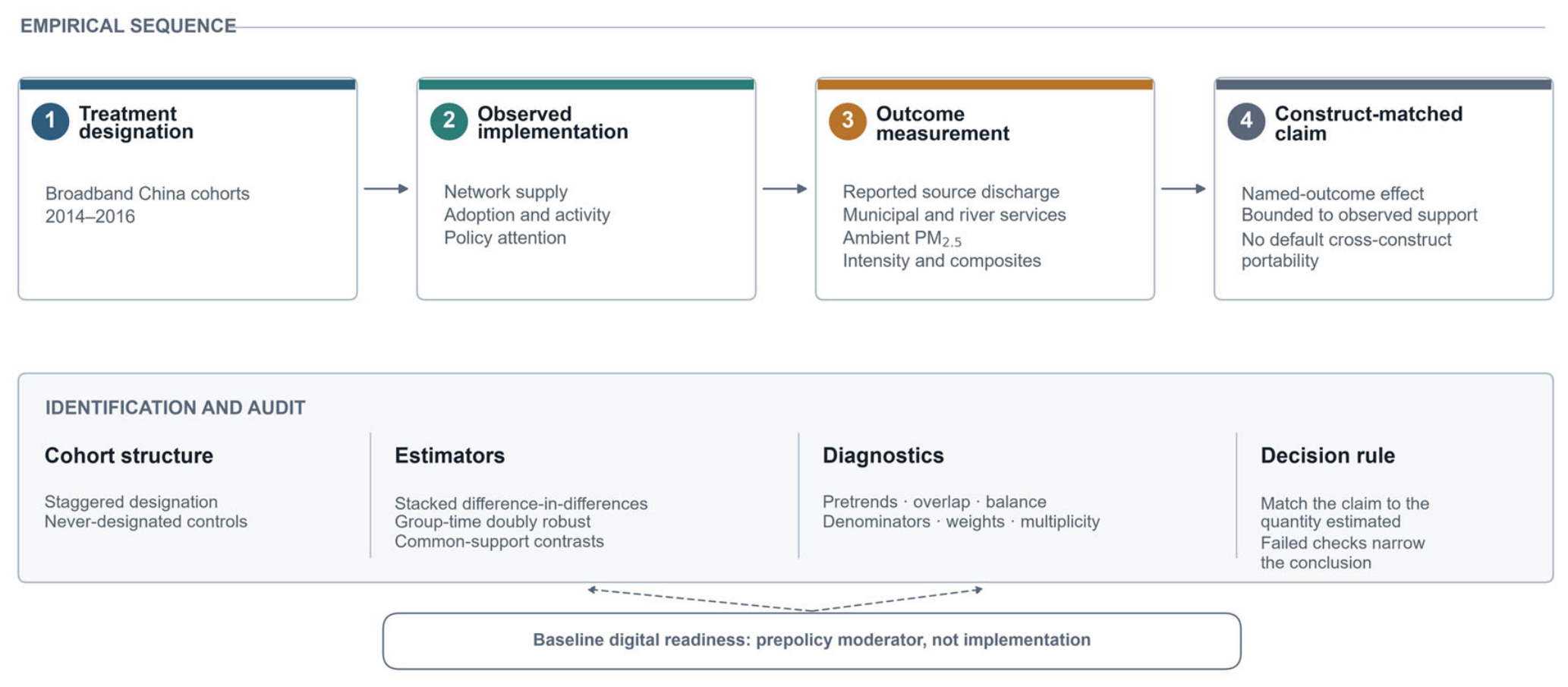
Figure 1 shows the logic in one sequence. Official designation defines exposure. The implementation gate tests whether attention, networks, or adoption changed as expected. The outcome audit then separates reported discharge, public services, ambient concentration, intensity, and composites. Estimators and diagnostics determine how far each conclusion can be carried. Baseline digital readiness enters only as a prepolicy conditioning capacity.

2.3. Baseline Digital Readiness as a Conditioning Capacity

The same designation can produce different responses because cities enter the program with different capacities to absorb, coordinate, and use digital infrastructure. Organizational adjustment, innovation, industrial control, user skills, and communications activity are complementary inputs rather than automatic consequences of designation. Existing Broadband China studies report heterogeneity by city type, region, urbanization, and regulatory intensity, but those categories do not directly measure prepolicy communications and adoption capacity.

We therefore use 2011–2013 mobile subscriptions, internet users, and telecom revenue per resident to measure baseline digital readiness. In this paper, the term means prepolicy communications adoption and activity capacity. It does not mean post-designation construction, network speed, latency, reliability, industrial digitalization, or service quality. Readiness is consequently a moderator, not the treatment first stage.

Let D_i denote standardized baseline readiness and T_ig membership in designation cohort g. A negative coefficient on T_ig × D_i for a reported-emissions long change is consistent with efficiency or abatement responses becoming stronger as readiness rises. A positive coefficient is consistent with readiness amplifying activity or reporting. Neither sign identifies the channel without intermediate outcomes.

We report the full interaction gradient, conditional policy contrasts, confidence intervals, and observed readiness support. The gradient tests whether one average masks systematic variation across baseline capacity. It does not establish a significant designation effect at every readiness value or identify a mechanism by itself.

2.4. Outcome Construction and Construct Portability

Composite environmental indices can summarize multidimensional performance, but their meaning depends on the conceptual framework, normalization, weighting, and aggregation procedure [26]. Sensitivity-based weighting makes it explicit that a plausible index is not determined by the data alone [27]. Min/max thresholds can also create implicit reweighting even when nominal weights do not change [28]. Environmental applications therefore recommend comparing alternative weighting procedures [29], whereas specification-curve logic favors a bounded, disclosed choice set with joint inference rather than selection of a preferred result [30].

We apply these principles to the three industrial components. Let $Z_{it}^W$, $Z_{it}^S$, and $Z_{it}^D$ denote within-year standardized log wastewater, sulfur dioxide, and smoke/dust. For nonnegative weights that sum to one,

$$P_{it}\left(w\right)=w_W Z_{it}^W+w_S Z_{it}^S+w_D Z_{it}^D, w_W+w_S+w_D=1$$

(2)

The analysis evaluates the complete 0.05 weight grid together with pooled raw, pooled log, and year-specific entropy variants. All weighting and transformation variants in this grid are retained and reported uniformly. Equation (2) defines the industrial composites, and the Section 4 summarizes the full grid.

GDP-based intensity raises a different problem. Let PM_it denote annual PM_2.5 and GDP_it real gross domestic product. Define

$$I_{it}=\mathrm{l}\mathrm{o}\mathrm{g}\left({PM}_{it}\right)-\mathrm{l}\mathrm{o}\mathrm{g}\left({GDP}_{it}\right)$$

(3)

In a linear fixed-effects model estimated on identical rows, the policy coefficient for I_it equals the PM_2.5 coefficient minus the GDP coefficient. A decline in I_it is therefore a decline in pollution intensity, not necessarily a decline in ambient concentration. The denominator is part of the estimand rather than a neutral scaling choice.

Within the outcome audit, comparisons are prioritized on common support. Dependence on weights, denominators, or processing rules must be reported when a conclusion is intended to represent a common environmental response. Changes in source coverage or observational unit define separate-support extensions; they locate a portability boundary but cannot attribute the difference to measurement alone.

2.5. Ambient Outcomes, Concurrent Policies, and Empirical Expectations

Annual PM_2.5 integrates sectors, fuels, atmospheric transport, and spatial processes [31]. ChinaHighPM_2.5 provides a long-run, high-resolution series suitable for city-boundary reaggregation [32], using satellite, meteorological, topographic, land-use, and emissions information [33].

The release used here is archived as a versioned data product [34]. High-resolution exposure research illustrates why modeled ambient concentration and an administrative discharge series are distinct measurement systems [35], while city-boundary harmonization remains part of the spatial definition [36].

Broadband China also overlaps major environmental-policy changes. Clean-heating policies produced identifiable air quality gains that should not be attributed to broadband designation [37], and national clean-air policies generated substantial effects outside the digital-policy estimand [38]. Year effects absorb common shocks but do not prove that all city-specific time-varying confounding has disappeared. The analysis therefore reports sensitivity to four concurrent environmental policies and limits causal language when policy selection, pretrends, overlap, or balance remain unresolved.

These expectations produce a fixed decision sequence: verify the named implementation stage, compare environmental outcomes on common support, and interpret readiness heterogeneity only over observed support. A failed pretrend, multiplicity, overlap, or balance criterion narrows the relevant claim; a significant coefficient in another construct does not repair it.

3. Materials and Methods

3.1. Policy Designation and Study Panel

Broadband China was a national demonstration program implemented in three city cohorts beginning in 2014, 2015, and 2016. The 2014 cohort is taken from the joint Ministry of Industry and Information Technology (MIIT) and National Development and Reform Commission (NDRC) notice [39]. The corresponding official list defines the 2015 cohort [40].

The 2016 cohort is defined by the final official notice [41]. Together, the notices describe a city application, provincial pre-review, and expert assessment process. “Pilot” therefore means official demonstration-city designation, not random assignment and not verified network completion.

The city crosswalk contains 119 named units in the three notices and directly matches 109 prefecture-level cities to the administrative panel: 37 in 2014, 36 in 2015, and 36 in 2016. City groups, districts, counties, and other non-equivalent units are not included in the prefecture-level analytical sample. The treatment year is the first designation year. Cities never designated during the outcome window form the comparison pool; already treated cities are not used as controls for later cohorts.

3.2. Realized Implementation and Baseline Digital Readiness

We evaluate realized implementation at three observed stages: government attention, physical-network supply, and adoption or activity. Attention is measured using digital-infrastructure language in municipal work reports; physical supply from fiber density and access ports; and adoption or activity from subscriptions and telecom revenue. We do not combine these measures because movement at one stage does not prove movement at another.

The published reference composite cannot be reproduced because its component weights are unavailable. Fiber density and access ports therefore form the primary physical-network family. The reference and equal-weight composites are retained only as secondary checks and are interpreted together with their pretrend and multiplicity diagnostics.

Baseline digital readiness combines mobile subscriptions, internet users, and telecom revenue per resident during 2011–2013. Each component is transformed as log(1 + x), averaged across the three years, standardized, and equally weighted. The index covers 273 cities, including 103 designated cities, and has mean zero and standard deviation one. It correlates 0.952 with a rank-based index and more than 0.999 with the first principal component, which explains 89.8% of component variance. Leave-one-component variants preserve the same interpretation. The index measures prepolicy communications adoption and activity capacity, not post-designation network quality.

3.3. Environmental Outcomes and Construction Choices

Annual industrial wastewater, sulfur dioxide, and smoke/dust measures come from national, provincial, and prefecture-level statistical yearbooks, including CSMAR and Guoyan records. The primary estimates use recorded log(1 + x) values. As a robustness check, conventional linear interpolation is applied only to eligible gaps bounded by observed values within the same city series; endpoints are not extrapolated. An additional wastewater series matches 4741 of 4742 overlapping city-years. The two series are treated as complementary coverage checks because they originate from the same statistical reporting system.

Municipal sewage volume and sewage-treatment rates describe the urban wastewater system. They do not measure industrial pollutant mass. To compare industrial and municipal series without forming a unit-dependent physical ratio, we define

$$C_{it}=\mathrm{l}\mathrm{o}\mathrm{g}(1+W_{it}^{\mathrm{i}\mathrm{n}\mathrm{d}\mathrm{u}\mathrm{s}\mathrm{t}\mathrm{r}\mathrm{i}\mathrm{a}\mathrm{l}})-\mathrm{l}\mathrm{o}\mathrm{g}(1+W_{it}^{\mathrm{m}\mathrm{u}\mathrm{n}\mathrm{i}\mathrm{c}\mathrm{i}\mathrm{p}\mathrm{a}\mathrm{l}})$$

(4)

A positive coefficient for C_it means that the industrial series rises proportionally more than the municipal series. It does not identify a change in river pollution.

Equation (4) is a proportional contrast between two administrative series; it is not a physical conversion between their original units.

Annual PM_2.5 is aggregated from the 1 km ChinaHighPM_2.5 Version 4 product. Zenodo record 3,539,349 covers 2000–2021, and record 15,208,529 covers later years. Grid cells are assigned to prefecture boundaries from DataV GeoAtlas Area v3. The main ambient panel covers 2011–2023.

Annual temperature, precipitation, humidity, and wind are aggregated from NASA POWER daily meteorological series queried at city centroids [42]. Concentrations are expressed in μg m⁻³. Sansha is not included because its prefecture polygon contains no valid land grid cell after boundary assignment.

River-quality measures are drawn from version 4 of the Lin et al. Figshare dataset. The dataset comprises weekly inland-water records from the China National Environmental Monitoring Centre. The main analysis uses a balanced annual city panel of the permanganate index, COD_Mn. A station-week weighted design is reported separately because it targets a different observational unit.

Mobile-Subscription–PM_2.5 Construct-Boundary Analysis

The mobile-subscription analysis is retained as a construct-boundary check rather than evidence of policy implementation. It uses the 2011–2019 city panel and a fixed 32-model grid crossing four sample rules, four covariate rules, and two fixed-effect rules. The primary model relates mobile subscriptions per 100 residents to annual PM_2.5 with weather controls and city and year fixed effects; inverse-probability weighting, balanced-panel, province-year, spatial–temporal, and lagged-exposure variants test sensitivity. Equivalence is evaluated at prespecified elasticities of ±0.05 and ±0.03. These bounds test whether the confidence interval excludes elasticities larger than 5% or 3% in absolute value; they are sensitivity thresholds, not universal cutoffs for policy relevance. This analysis concerns one adoption measure and one ambient outcome; it is not a test of digital infrastructure in general.

3.4. Data Sources, Preprocessing, and Sample Construction

Table 1. Data sources and variable definitions.

Variable Group	Measure (Original Unit)	Coverage Used in Analysis	Source	Analytical Role
Policy designation	Broadband China designation; binary status	2014, 2015, and 2016 cohorts; 119 named units and 109 directly matched prefecture-level cities	Archived MIIT–NDRC cohort notices and city crosswalk	Treatment timing
Adoption and activity	Subscriptions per 100 residents; telecom revenue per resident	2005–2019; 297–298 cities; 109 designated cities	National and subnational statistical yearbooks and licensed CSMAR/Guoyan records	Adoption and communications activity
Physical network	Long-distance fiber per area; access ports per resident	2006–2019 estimation window; 283 cities; 107 designated cities	City statistical panel	Implementation measure
Government attention	Keyword occurrences per 10,000 report words	2007–2019; 282 cities; 105 designated cities	Municipal government work reports	Agenda salience
Industrial discharge	Wastewater (10,000 tonnes); sulfur dioxide and smoke/dust (tonnes)	Main estimates use 2005–2019 or shorter common-support windows; up to 297 cities and 109 designated cities	National-, provincial-, and prefecture-level statistical yearbooks, including licensed CSMAR/Guoyan access	Reported source quantities; log(1 + x) in regressions
Municipal wastewater	Sewage volume (10,000 m3); treatment rate (%)	2005–2019; up to 292 cities and 108 designated cities	National-, provincial-, and prefecture-level statistical yearbooks, including licensed CSMAR/Guoyan access	Municipal service outcomes
Ambient air	Annual PM2.5 (μg m−3)	2011–2023; 296 cities; 109 designated cities	ChinaHighPM2.5 V4 grids aggregated to prefecture polygons	Ambient concentration
River quality	Permanganate index (CODMn; mg L−1)	2007–2018; 133 stations in 98 cities and 47 designated cities	Lin et al. Figshare V4 inland-water records	Ambient water quality

consolidates definitions, sources, analytical roles, and coverage. Administrative and implementation models stop in 2019 to preserve a definition-consistent pre-pandemic window; later observations could mix the policy response with pandemic disruption and changes in administrative reporting. Accordingly, the main analysis windows are 2005–2019 for administrative outcomes, 2006–2019 for physical networks, 2007–2018 for river quality, and 2011–2023 for annual PM_2.5. The extended PM_2.5 panel is a separate ambient check rather than part of the four-outcome common-support design.

The primary models use recorded observations, and each construct is analyzed on its available support. The interpolation check described in Section 3.3 is kept separate from the primary analytical sample. Table 1 defines each measure and its analytical role;

Table 2. Sample formation and wastewater event-time support.

Panel A. Main common-support sample formation.
Stage		Rows	Cities	Never Designated	2014 Cohort	2015 Cohort	2016 Cohort	Years
Administrative city outcome source		7425	297	188	37	36	36	2000–2024
Administrative rows with observed PM2.5 and weather		3848	296	187	37	36	36	2011–2023
Restricted common comparison window		2664	296	187	37	36	36	2011–2019
Complete common-support city-years		2427	294	186	37	36	35	2011–2019
Cohort-stacked estimation sample		5463	294	186	37	36	35	2011–2019
Panel B. Statistical yearbook industrial-wastewater group-time support.
Event time	Contributing cohorts	Treated city pairs		Treated pairs per cohort cell, min–max			Never-treated city pairs
−4	3	107		34–37			533
−3	3	107		34–37			537
−2	3	107		34–37			539
0	3	105		32–37			533
+1	3	101		31–37			519
+2	3	98		29–35			492
+3	3	94		27–36			458

Note: Stacking repeats never-designated cities across cohort comparisons and does not create new independent cities. City pairs require an observed outcome at the event year and the cohort-specific baseline year. Never-treated city pairs are cohort-specific comparison pairs, not unique cities. The source audit extends through 2024, but administrative outcome models stop in 2019 to preserve a definition-consistent pre-pandemic estimation window.

and

Table 3. Descriptive statistics for the 2427-city-year common-support sample.

Variable	N	Mean	SD	P25	P50	P75	Min	Max
log(1 + industrial wastewater)	2427	8.141	1.198	7.542	8.272	8.907	0.693	11.477
log(1 + industrial SO2)	2427	10.029	1.239	9.297	10.137	10.916	1.099	13.183
log(1 + industrial smoke/dust)	2427	9.694	1.183	8.999	9.779	10.482	2.485	15.458
ln(annual PM2.5)	2427	3.811	0.348	3.569	3.799	4.058	2.701	4.720
Temperature (°C)	2427	13.873	5.395	10.155	15.213	17.175	−3.410	25.617
ln(precipitation)	2427	6.787	0.625	6.395	6.831	7.283	3.125	7.897
Relative humidity (%)	2427	70.923	11.145	63.091	73.705	80.326	27.293	88.512
Wind speed (m s−1)	2427	3.350	0.734	2.897	3.369	3.741	1.295	5.534
Smart-city policy active	2427	0.410	0.492	0	0	1	0	1
Low-carbon policy active	2427	0.360	0.480	0	0	1	0	1
Broadband China designated city	2427	0.375	0.484	0	0	1	0	1
Broadband China designation active	2427	0.201	0.401	0	0	0	0	1

Note: SD denotes standard deviation; P25, P50, and P75 denote the 25th, 50th, and 75th percentiles. Descriptive statistics use the identical 2011–2019 city-years for the four cross-outcome comparisons. Logged industrial quantities use log(1 + x); industrial wastewater is measured in 10,000 tonnes, SO₂ and smoke/dust in tonnes and PM_2.5 in μg m⁻³ before transformation.

then show how those choices determine the sample, event-time support, and common-sample distribution.

Sample Construction and Event-Time Support

Sample construction is reported before outcome comparison. The source audit contains 7425 city-years for 297 cities during 2000–2024. Matching PM_2.5 and weather leaves 3848 city-years for 296 cities, and restricting the comparison window to 2011–2019 leaves 2664. Requiring four outcomes, four weather variables, and two concurrent-policy indicators yields the common 2427-city-year panel for 294 cities: 186 never designated and 108 designated. Cohort sizes are 37, 36, and 35. Stacking cohorts creates 5463 rows but no additional independent cities.

All three cohorts contribute to wastewater event times from −4 to +3. Treated city pairs decline from 107 to 94 as outcome availability changes. Table 2 reports this support so that a stable event-study line is not mistaken for constant composition.

Table 3 reports N, mean, standard deviation, quartiles, and range for every variable in the common-support comparison.

3.5. Estimands and Estimation

3.5.1. Group-Time Estimand

For cohort $g$ and year $t$, define ${\Delta Y}_{i,g,t}=Y_{it}-Y_{i,g-1}$. Under no anticipation and parallel untreated changes, the following never-designated-group contrast identifies $\mathrm{A}\mathrm{T}\mathrm{T}(g,t)$:

$$\mathrm{A}\mathrm{T}\mathrm{T}(g,t)=\mathrm{E}[{\Delta Y}_{i,g,t} | G_i=g]-\mathrm{E}[{\Delta Y}_{i,g,t} | G_i=\infty ]$$

(5)

G_i denotes the first designation year, and G_i = ∞ denotes a never-designated city. We aggregate event years 0 through 3, weighting cohorts by treated-city counts. The estimator follows the group-time logic for multiple treatment periods [43]. It avoids using already treated cities as controls.

The group-time interpretation requires no anticipation, parallel untreated changes, stable units, nonselective outcome availability conditional on design variables, and adequate comparison support. Because assignment followed city application and review, spillovers and unobserved selection remain possible. We therefore treat leads, sample counts, overlap, and balance as diagnostics and report unadjusted and doubly robust estimates side by side; a failed diagnostic narrows the result to a policy-associated contrast.

Heterogeneous timing can make conventional two-way fixed-effects event studies difficult to interpret [44]. Related event-study estimands address treatment-effect heterogeneity [45]. The group-time estimator is therefore primary; stacked fixed-effects models are retained only as transparent benchmarks [46].

3.5.2. Stacked Benchmark and Event Time

For cohort stack c,

$$Y_{ict}={\alpha }_{ic}+{\lambda }_{ct}+\beta D_{ict}+{\epsilon }_{ict}$$

(6)

where D_ict equals one for a cohort city in and after its designation year. Stack-city and stack-year fixed effects are absorbed. Never-designated cities can appear in multiple stacks, so standard errors cluster by original city; province-by-year effects are a sensitivity. Equation (6) is a replication benchmark. Event year −1 is the omitted reference, and every lead or lag is interpreted relative to it [47]. Event-study guidance also motivates reporting the complete dynamic path [48]. A non-rejected pretrend is a diagnostic, not proof of parallel trends [49].

3.6. Selection Adjustment

Pilot designation was not random. We therefore estimate a cross-fitted doubly robust group-time model. Let $e_g\left(X_i\right)=P(G_i=g | G_i\in \{g,\infty \},X_i)$, $m_{0,g,t}\left(X_i\right)=E[{\Delta Y}_{i,g,t} | G_i=\infty ,X_i]$, ${\omega }_{ig}={\displaystyle \frac{e_g\left(X_i\right)}{1-e_g\left(X_i\right)}}$, and $u_{i,g,t}={\Delta Y}_{i,g,t}-m_{0,g,t}\left(X_i\right)$. The nuisance models use pre-designation GDP, secondary-industry share, baseline outcomes, pretreatment trends, sulfur dioxide, and smoke/dust; all predictions are obtained out of fold. The estimator is

$${\widehat{\mathrm{A}\mathrm{T}\mathrm{T}}}^{\mathrm{D}\mathrm{R}}(g,t)={\displaystyle \frac{1}{N_g}}\sum _{i:G_i=g}{\widehat{u}}_{i,g,t}-{\displaystyle \frac{{\displaystyle \sum _{i:G_i=\infty }}{\widehat{\omega }}_{ig}{\widehat{u}}_{i,g,t}}{{\displaystyle \sum _{i:G_i=\infty }}{\widehat{\omega }}_{ig}}}$$

(7)

Cross-fitting separates nuisance-model estimation from evaluation. We report maximum propensities and weighted standardized mean differences. The estimator adjusts for observed selection under the stated models but does not remove unobserved time-varying confounding.

Extreme propensities make an ATT depend on extrapolation, so we also estimate an overlap-population effect. Treated observations receive weight 1 − e(X), and controls receive e(X). The overlap gate requires a maximum propensity below 0.98, a maximum weighted standardized difference no greater than 0.10, adequate effective sample sizes, and no excessive normalized weight.

3.7. Exploratory Baseline-Readiness Heterogeneity Analysis

The readiness analysis fixes industrial smoke/dust as the outcome and replaces polynomial treatment-specific time trends with a cohort-specific long difference. For cohort g ∈ {2014, 2015, 2016},

$${\Delta Y}_{ig}={\displaystyle \frac{1}{4}}{\displaystyle \sum _{t=g}^{g+3}}\mathrm{l}\mathrm{o}\mathrm{g}(1+{SmokeDust}_{it})-{\displaystyle \frac{1}{3}}{\displaystyle \sum _{t=g-3}^{g-1}}\mathrm{l}\mathrm{o}\mathrm{g}(1+{SmokeDust}_{it})$$

(8)

The treated group contains cities first designated in cohort g; controls are never-designated cities. Each cohort uses the same three-year pre-period and four-year post-period. We estimate

$${\Delta Y}_{ig}={\alpha }_{pg}+\beta T_{ig}+\gamma D_i+\theta (T_{ig}\times D_i)+X_i^{\prime }\delta +{\epsilon }_{ig}$$

(9)

where α_pg are province-by-cohort fixed effects and D_i is baseline digital readiness. X_i contains the prepolicy smoke/dust mean and slope, sulfur dioxide and industrial-wastewater means, GDP per capita, secondary-industry share, science spending per capita, ICT employment intensity, and environmental/public-facilities employment intensity.

Cohort-specific propensity scores define overlap weights normalized within cohort and treatment status. The target is the differential long change associated with one standard deviation of readiness. Inference clusters by city; province clustering and a 999-draw Webb bootstrap assess sensitivity to the smaller assignment-level cluster count.

The readiness module is evaluated within the same city database and is therefore classified as an exploratory within-sample heterogeneity analysis rather than an independent confirmation. The reported diagnostic set includes a prepolicy placebo, a common-support restriction, unweighted estimation, leave-one-province and leave-one-cohort specifications, a specification omitting the 2016–2017 reporting-transition years, and a quadratic readiness term.

The same design is applied to five fixed mechanism outcomes. Province-cluster Webb p-values are adjusted using the Benjamini–Hochberg false-discovery rate; no estimate is interpreted as mediation unless it passes the family correction and the relevant measurement gates.

3.8. Inference, Multiplicity, and Decision Rules

Cluster choice follows the assignment and data structure [50], and established cluster-robust guidance informs implementation [51]. Group-time estimates use 999 city-stratified bootstrap draws and simultaneous bands based on the maximum absolute t statistic. Sensitivity to the finite number of provinces uses a null-restricted Webb bootstrap [52]. A fast cluster-bootstrap procedure is also reported [53]. The province-stratified permutation is reported as a conditional placebo and interpreted under the stated within-province exchangeability condition.

Unknown cross-sectional dependence remains a general panel-data concern [54]. Conley-style spatial–temporal inference is retained for the mobile-subscription–PM_2.5 boundary analysis [55].

We report nominal significance, family adjustment, pretrends, overlap, and balance separately. Passing one criterion does not offset failure of another. The corresponding implementation and outcome tables report support, uncertainty, and sensitivity alongside each result.

3.8.1. Source-Level Inference and Analytical Units

Analysis populations, variable availability, assumptions, and sensitivity rules are reported together [56]. Province-level aggregates are not used as city observations because they do not provide independent city-level variation [57].

3.8.2. Interpretation Rules

Every claim is matched to its estimand. Evidence for one outcome supports only that outcome, and a broader environmental interpretation must survive the component, denominator, and aggregation audits. Same-support comparisons hold city-years fixed; separate-support modules identify an external boundary rather than a measurement-only difference.

3.9. Reporting Transparency and Auditability

The analyses report the definitions, support, diagnostics, and sensitivity families underlying the manuscript claims. The replication code uses Python 3.11 or later, NumPy 1.26 or later, pandas 2.1 or later, and statsmodels 0.14 or later. No physical equipment or laboratory materials were used. This audit-oriented reporting draws on FAIR principles [58] and reproducibility guidance [59] while distinguishing transparent documentation from unrestricted public access [60].

4. Results

4.1. Implementation Gate: No Reliable Physical-Network First Stage

The implementation gate fails before the environmental comparison begins. Fixed-broadband subscriptions are lower and fail the pretrend test; telecom revenue and internet subscriptions are imprecise; and mobile subscriptions and the digital-activity index are negative, with the mobile series also showing a differential pretrend. These estimates are more consistent with selection or different baseline trajectories than with a designation-induced contraction.

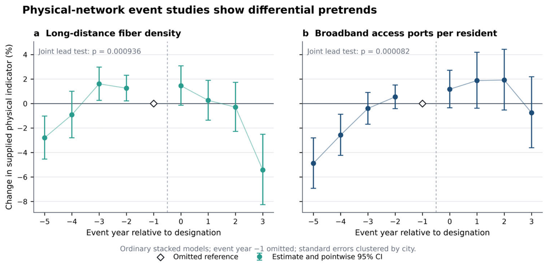
Physical-network results do not repair the first stage. Access ports increase by 3.79% (95% confidence interval: 1.42% to 6.21%), while fiber changes little, but both event studies fail the joint pretrend test. Selection-adjusted fiber estimates then fail overlap or balance checks, and overlap-weighted estimates remain near zero with residual imbalance.

Government attention also provides no reliable implementation signal. The two measures are imprecise and disagree in sign; the core measure fails its pretrend test, and a 3.02-percentage-point report-availability difference adds a missingness warning.

Table 4. Treatment-construct estimates and declared interpretation criteria.

Construct/Estimator	Estimate (95% CI)	p; q; Pretrend p	Overlap/Balance	Failed Criterion
Broadband per 100 permanent residents	−14.04% *** ([−20.87, −6.61])	0.0004; —; 0.0031	—	Sign; pretrend
Broadband per 100 registered residents	−8.51% ** ([−14.97, −1.56])	0.0179; —; 0.114	—	Sign
Fiber density, stacked	−0.58% ([−2.36, 1.24])	0.532; 0.532; 0.00094	—	Precision; pretrend
Access ports, stacked	+3.79% *** ([1.42, 6.21])	0.00179; 0.00359; 0.000082	—	Pretrend
Reference physical index	+0.129 ** SD ([0.002, 0.256] SD)	0.0480; 0.0830; 0.0218	—	FDR; pretrend
Six-component equal-weight index	+0.066 * SD ([−0.004, 0.135] SD)	0.0646; 0.0830; 0.208	—	Precision
Fiber density, doubly robust ATT	+8.55% ** ([0.85, 16.90])	0.0183; 0.0366; 0.212	max e(X) = 0.99999; max |SMD| = 1.522	Overlap; balance
Access ports, doubly robust ATT	+13.64% ([−1.05, 30.59])	0.1008; 0.1008; 0.111	max e(X) = 0.99999; max |SMD| = 1.522	Precision; overlap; balance
Fiber density, overlap population	+1.03% ([−0.80, 2.91])	0.306; 0.441; 0.573	max |SMD| = 0.328	Precision; balance
Access ports, overlap population	+1.14% ([−1.37, 3.74])	0.441; 0.441; 0.245	max |SMD| = 0.328	Precision; balance
Broad report attention	−7.53% ([−17.41, 3.52])	0.175; 0.350; 0.123	—	Positive first stage
Core report attention	+1.80% ([−7.48, 12.00])	0.715; 0.715; 0.00148	—	Precision; pretrend

Note: Three, two, and one asterisk denotes nominal significance at the 1%, 5%, and 10% levels, respectively; they do not override adjusted q-values or design gates. Logged components are reported as percentage changes and standardized indices as standard deviations. A primary implementation result must pass direction, family-adjustment, pretrend, overlap, and balance criteria where applicable. ATT denotes the average treatment effect on the treated; FDR, false-discovery rate; SMD, standardized mean difference. Estimate and diagnostic details are reported in the table.

summarizes this decision: designation is observed, but a reliable physical-network response is not. The remaining analysis therefore evaluates the environmental consequences of designation and does not label them as effects of verified network improvement. We begin by holding city-years fixed across outcomes.

4.2. Common-Support Outcomes Do Not Support One Environmental Response

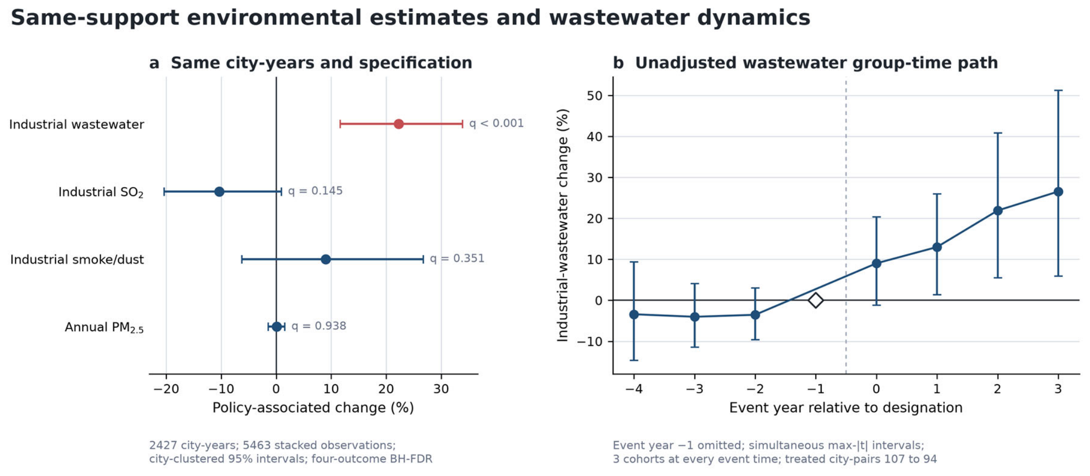
Industrial wastewater is the only precise positive result in the common-support outcome audit. In the primary group-time design, it rises by 17.15% over event years 0–3 (95% bootstrap interval: 8.58% to 26.59%; pre-period p = 0.293), increasing from 9.03% at designation to 26.56% at event year 3. Figure 2 shows this dynamic path.

The same conclusion appears in the fixed 2427-city-year comparison: industrial wastewater rises by 22.26% (95% confidence interval: 11.63% to 33.89%; q = 0.00008), whereas sulfur dioxide, smoke/dust, and PM_2.5 are imprecise after family adjustment. The comparison therefore does not support an outcome-invariant environmental conclusion.

Province-level Webb and within-province permutation checks retain the wastewater signal, and all reported alternative specifications remain positive, ranging from 14.61% to 22.18%. These results indicate stability across the reported specifications; the selection-adjusted analysis is considered separately in Section 4.3.

4.3. Selection Adjustment Weakens the Wastewater Estimate

Selection adjustment materially weakens the wastewater estimate. On the adjusted sample, the unadjusted estimate is 16.45%, while the cross-fitted doubly robust estimate is 7.69% (95% multiplier interval: −2.09% to 18.43%; p = 0.130). The maximum propensity is 0.906, but weighted imbalance reaches 0.361. The defensible conclusion is therefore a selection-sensitive policy-associated increase, not a gate-passing causal magnitude.

Entropy balancing produces a descriptive estimate of +12.19%, but concentrated 2014 control weights fail the declared reliability criterion. Because alternative estimators do not remove the selection concern, the next comparison asks what the wastewater measure itself represents.

Table 5. Environmental component and selection-adjusted estimates.

Outcome and Estimator	Estimate (95% Interval)	p; Pretrend p	Sample/Inference
Industrial wastewater, group-time	+17.15% *** ([8.58, 26.59])	0.001; 0.293	12 cohort-horizon cells; treated pairs 105 (h = 0), 94 (h = 3); city-stratified percentile bootstrap
Industrial wastewater, doubly robust	+7.69% ([−2.09, 18.43])	0.130; —	196/172/144 cities by cohort; cross-fitted multiplier bootstrap
Industrial SO2, group-time	−8.28% ([−18.40, 2.15])	0.124; 0.101	12 cohort-horizon cells; 294-city common panel; city-stratified percentile bootstrap
Industrial smoke/dust, group-time	+10.79% ([−2.67, 25.04])	0.120; 0.706	12 cohort-horizon cells; 294-city common panel; city-stratified percentile bootstrap
Municipal sewage, stacked	−2.25% ([−8.48, 4.42])	0.500; —	9852 stacked observations; 292 cities; city-clustered Wald interval
Industrial minus municipal, group-time	+19.14% *** ([8.73, 30.34])	0.001; 0.573	12 matched industrial–municipal cells; city-stratified percentile bootstrap
Industrial minus municipal, doubly robust	+6.93% ([−6.04, 21.64])	0.306; —	196/172/144 cities by cohort; cross-fitted multiplier bootstrap
Annual PM2.5, full 2011–2023	−0.74% ([−2.65, 1.22])	0.458; —	8710 stacked observations; 296 cities; city-clustered Wald interval
CODMn, balanced annual city panel	+2.82% ([−4.51, 10.71])	0.463; —	1169 observations; 89 cities; city-clustered Wald interval
CODMn, station-week weighted	+8.19% ** ([0.99, 15.91])	0.0268; —	50,165 observations; 98 cities; station-clustered Wald interval

Note: Three and two asterisks denote nominal significance at the 1% and 5% levels, respectively. Interval methods are stated row by row because resampling and clustering follow different assignment or observational units. The two river rows must be read together because they differ in observational unit and weighting. Group-time models resample cities within cohort strata; stacked-city models cluster standard errors by city. Adjusted models use cohort-specific cross-fitting and inference from a 9999-draw city-level multiplier bootstrap. The station-week river model includes station and year fixed effects and clusters by monitoring station. Interpretive conclusions are stated in Section 4.2, Section 4.3, Section 4.4, Section 4.5, Section 4.6 and Section 4.7 rather than repeated in the table.

consolidates the environmental component and selection-adjusted estimates.

4.4. Industrial and Municipal Wastewater Measure Different Processes

Industrial discharge and municipal sewage do not show the same movement. Municipal sewage changes by −2.25% (95% confidence interval: −8.48% to 4.42%), while the industrial-minus-municipal contrast is 19.14% (bootstrap interval: 8.73% to 30.34%). The result is consistent with movement in the industrial reporting construct, not with a general expansion of urban wastewater volume.

Selection adjustment again weakens the contrast: the unadjusted estimate is 17.39%, but the doubly robust estimate is 6.93% (multiplier interval: −6.04% to 21.64%). Weighted imbalance reaches 0.571, leaving the adjusted contrast imprecise and outside the balance gate.

4.5. PM_2.5 Intensity Does Not Imply Lower Concentration

Changing the denominator changes the object being estimated. On identical 2011–2019 rows, PM_2.5 changes by −0.09%, GDP by 2.54%, and PM_2.5/GDP by −2.56%; all three estimates are imprecise. Across eight matched designs, the intensity coefficient equals the PM_2.5 coefficient minus the GDP coefficient to numerical precision. A lower PM_2.5/GDP estimate therefore cannot be read automatically as a lower ambient concentration.

4.6. Composite Conclusions Depend on Weights

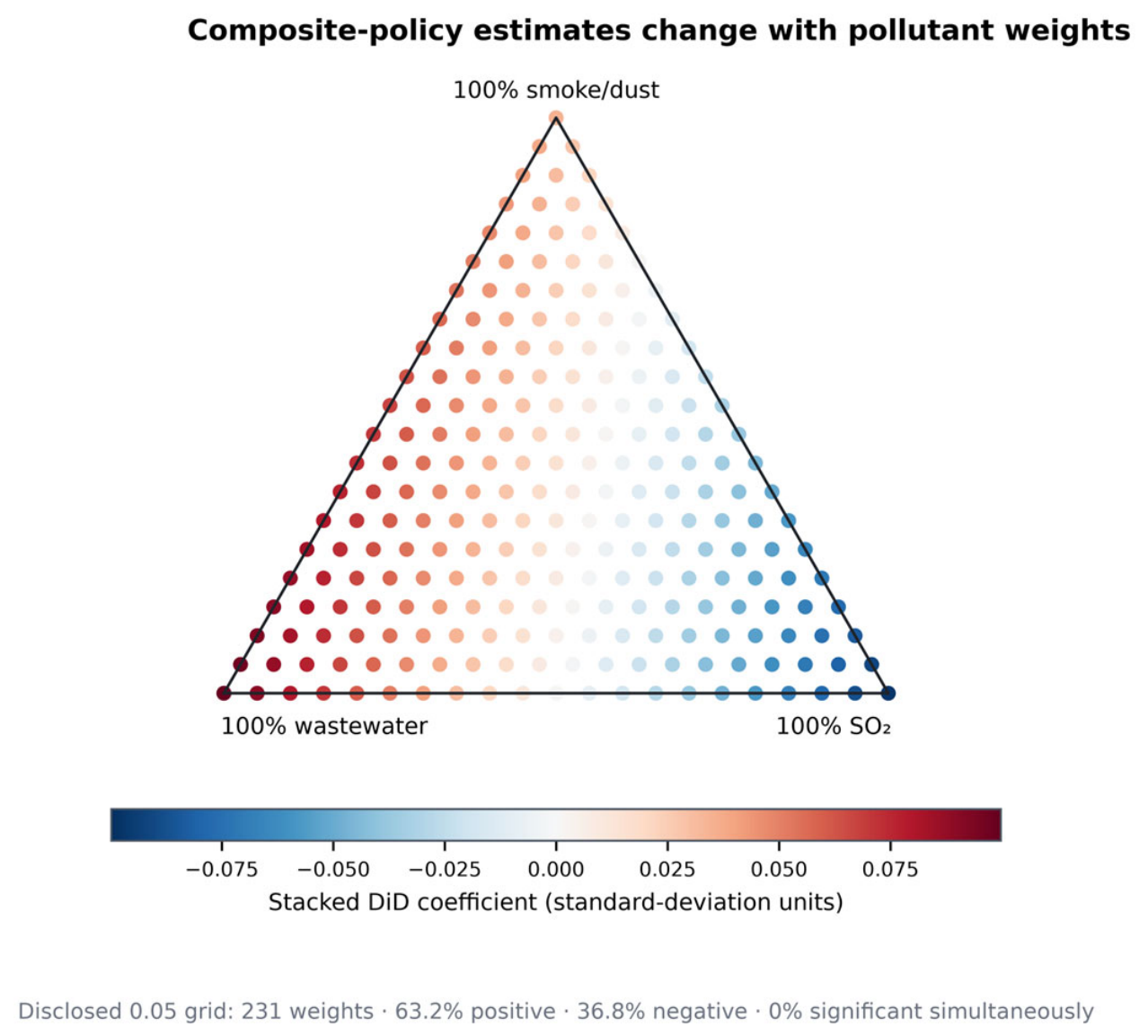
Composite results also depend on construction choices. The equal-weight industrial index is near zero. One raw-scale entropy index is pointwise negative but fails family adjustment, and the remaining entropy indices are imprecise. Across 231 nonnegative weight triples, 63.2% of estimates are positive and 36.8% are negative; only 3.03% are pointwise positive and significant, and none survives simultaneous inference. Figure 3 makes this weight dependence visible.

Table 6. Outcome construction and denominator audits.

Audit	Estimate or Surface Result	95% Interval or Estimate Range	p or q	Analysis Support
PM2.5 level, stacked 2011–2019	−0.09%	[−1.62, 1.46]	p = 0.906	5795 stacked observations; 296 cities
GDP denominator, same rows	+2.54%	[−1.90, 7.17]	p = 0.268	Same 5795 observations
PM2.5/GDP intensity, same rows	−2.56%	[−7.42, 2.55]	p = 0.321	Same 5795 observations
Equal-weight industrial index	+0.0123 SD	[−0.0872, 0.1119] SD	p = 0.808	9270 stacked observations; 294 cities
Pooled raw-value entropy index	−0.00603 **	[−0.01197, −0.00008]	p = 0.0479; q = 0.144	Same 9270 observations
Pooled log-entropy index	+0.00462	[−0.00429, 0.01352]	p = 0.310	Same 9270 observations
Year-specific raw entropy index	−0.00093	[−0.01228, 0.01042]	p = 0.873	Same 9270 observations
Full 231-weight simplex	63.2% positive; 36.8% negative	Estimate range [−0.0972, 0.0997]	0% simultaneous significance	Same 9270 observations; 231 fixed nonnegative weights

Note: Two asterisks denote nominal significance at the 5% level; the starred entropy estimate does not pass the reported family adjustment. All three denominator audit rows use identical 2011–2019 city-years, stack-by-city and stack-by-year fixed effects, and city-clustered standard errors. All industrial index rows use the common 2011–2019 component panel with the same fixed effects and city clustering. The simplex percentages describe the disclosed nonnegative weight grid; they do not treat the 231 estimates as independent experiments. Diagnostic conclusions are stated in Section 4.5 and Section 4.6.

summarizes the outcome-construction and denominator audits discussed in Section 4.5 and Section 4.6.

4.7. Ambient and Subscription Results Remain Bounded

Separate ambient analyses locate the boundary of the administrative source results. Over 2011–2023, annual PM_2.5 changes by −0.74%, with a 95% confidence interval of −2.65% to 1.22%. At the sample geometric mean of 38.3 μg m⁻³, this corresponds to about −0.28 μg m⁻³. The interval is not interpreted as an equivalence test because no external equivalence threshold was specified.

The balanced annual city-level COD_Mn estimate is 2.82% and imprecise. A station-week weighted design gives 8.19%, with p = 0.0268. Because the observational unit and weights differ, the station-week result is reported alongside, not in place of, the balanced annual result.

The available mechanism variables do not identify a monitoring or disclosure channel. Pollution Information Transparency Index (PITI) scores do not rise after designation, automatic monitoring disclosure is imprecise, and treatment-rate availability changes differentially. Government report attention also lacks a reliable positive first stage. Monitoring, disclosure, enforcement, production scale, energy demand, and industrial composition therefore remain competing interpretations.

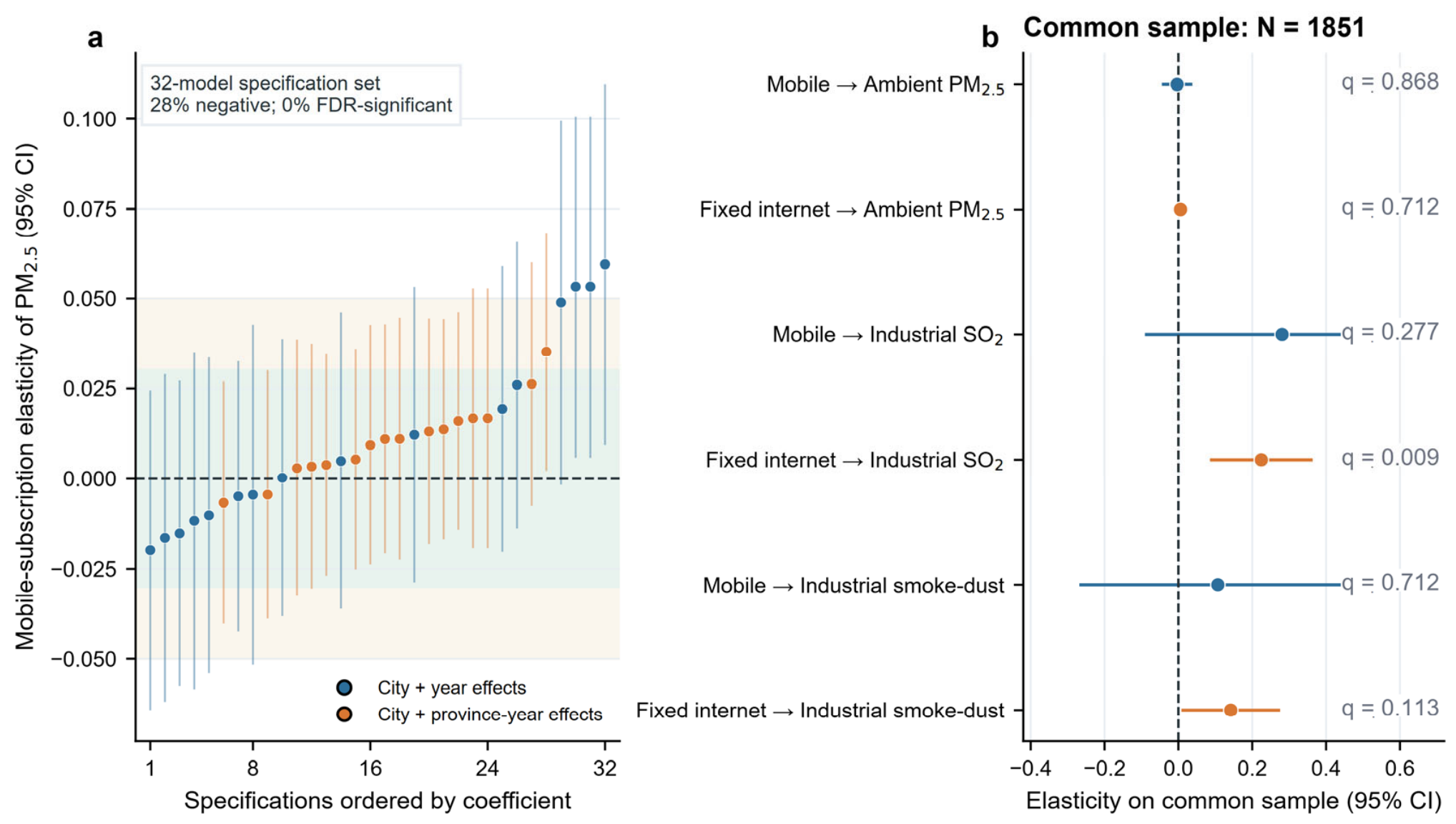
The mobile-subscription analysis is near zero at its stated construct level. The primary elasticity is 0.0050 (95% confidence interval: −0.0362 to 0.0461; p = 0.813), and the 32-model grid ranges from −0.020 to 0.059. Four nominal p-values fall below 0.05, but none survive family adjustment. Equivalence is supported at ±0.05 (p = 0.016) but not at ±0.03 (p = 0.117). This result bounds the association between one adoption measure and one ambient outcome; we next hold the outcome fixed and examine prepolicy capacity.

4.8. Exploratory Readiness Heterogeneity

The exploratory analysis holds smoke/dust fixed and tests whether the designation contrast varies with prepolicy communications capacity. It uses 488 cohort-stacked observations from 234 cities, including 79 designated cities in 29 provinces. The included covariate means are balanced, but support remains limited: the largest normalized weight is 7.72 and treated effective sample sizes range from 20.52 to 25.89 across cohorts.

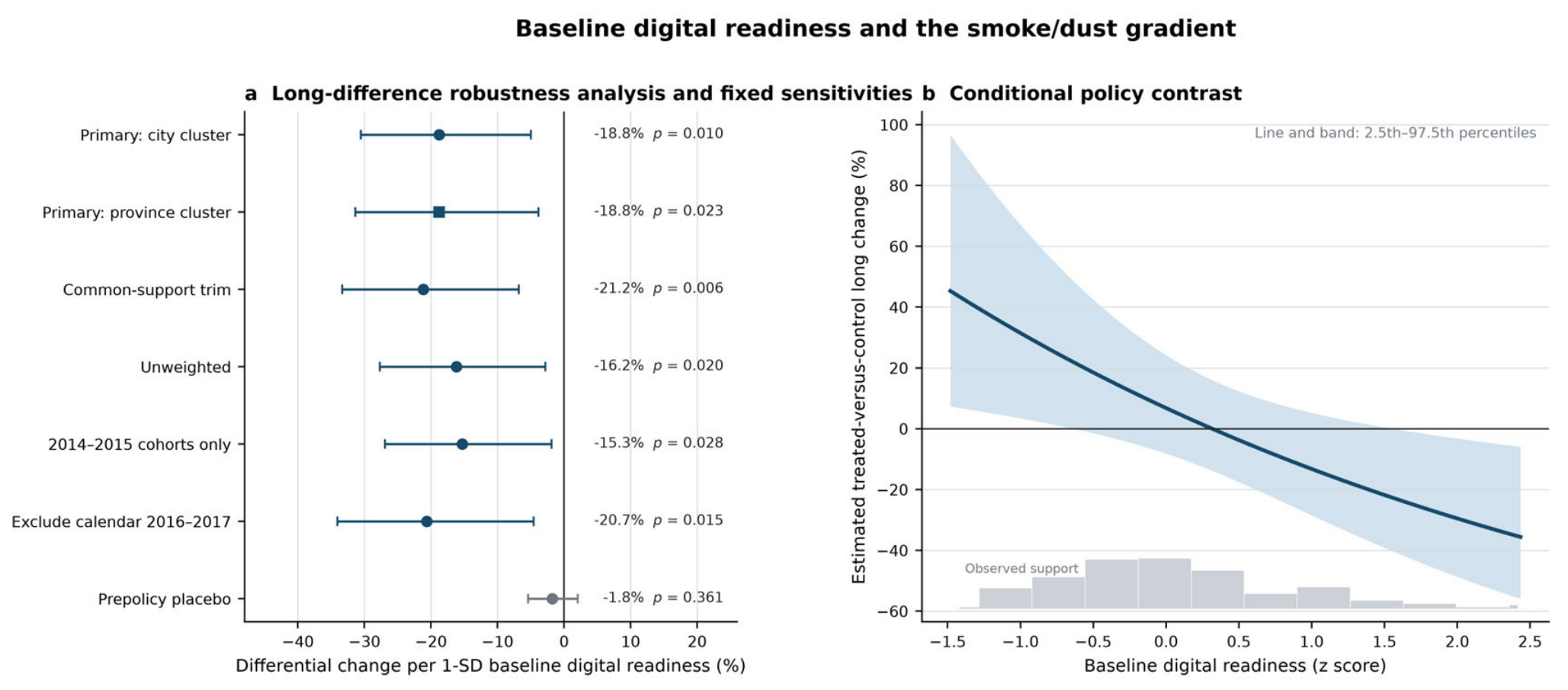
The readiness interaction is −0.2078: a one-standard-deviation increase is associated with an 18.76% lower treated-versus-control smoke/dust change (city-clustered 95% confidence interval: −30.54% to −4.98%; p = 0.0099). Province clustering leaves the coefficient unchanged (95% confidence interval: −31.37% to −3.83%; Webb p = 0.003).

This coefficient is a gradient, not the designation effect at a selected readiness value. The conditional contrast moves from 31.48% at one standard deviation below the mean to −13.23% at one standard deviation above it and equals 6.81% at the mean. Figure 4 therefore shows the full line, uncertainty band, and observed support.

Across the reported diagnostics, the prepolicy placebo is imprecise, the common-support restriction gives −21.17%, and all 29 leave-one-province estimates remain negative. Leave-one-cohort specifications and the sensitivity omitting the 2016–2017 reporting-transition years preserve the sign; the early-cohort restriction is less precise under province inference, and the quadratic term shows no curvature. These checks support a stable sample-specific association, not independent confirmation.

Table 7. Baseline-readiness long-difference robustness analysis and fixed diagnostics.

Specification	Differential Change per 1-SD Readiness	95% Confidence Interval	Inference	Support
Primary overlap weighted, city cluster	−18.76% ***	[−30.54%, −4.98%]	p = 0.0099	488 stacked observations; 234 cities; 79 designated
Primary overlap weighted, province cluster	−18.76% **	[−31.37%, −3.83%]	p = 0.0226; Webb p = 0.003	29 province clusters
Common-support restriction	−21.17% ***	[−33.33%, −6.79%]	p = 0.0059	375 observations; 214 cities; 73 designated
Unweighted	−16.17% **	[−27.68%, −2.83%]	p = 0.0200	Primary rows
2014–2015 cohorts only	−15.32% **	[−26.91%, −1.89%]	city p = 0.0278; province Webb p = 0.064	350 observations; 213 cities
Omit reporting-transition years 2016–2017	−20.67% **	[−34.06%, −4.55%]	city p = 0.0149; province Webb p = 0.003	Primary stacked rows; post-period averages recomputed over retained years
Policy pre-period placebo	−1.76%	[−5.41%, 2.04%]	city p = 0.3608; province Webb p = 0.323	Primary rows

Note: Three and two asterisks denote nominal significance at the 1% and 5% levels, respectively. The estimand is the differential smoke/dust long change associated with a one-standard-deviation increase in baseline digital readiness. It is not the policy effect evaluated at one readiness value. Overlap weights are cohort-specific and normalized within treatment status. City-clustered intervals are shown unless the row states province clustering.

reports the corresponding robustness estimates and fixed diagnostics.

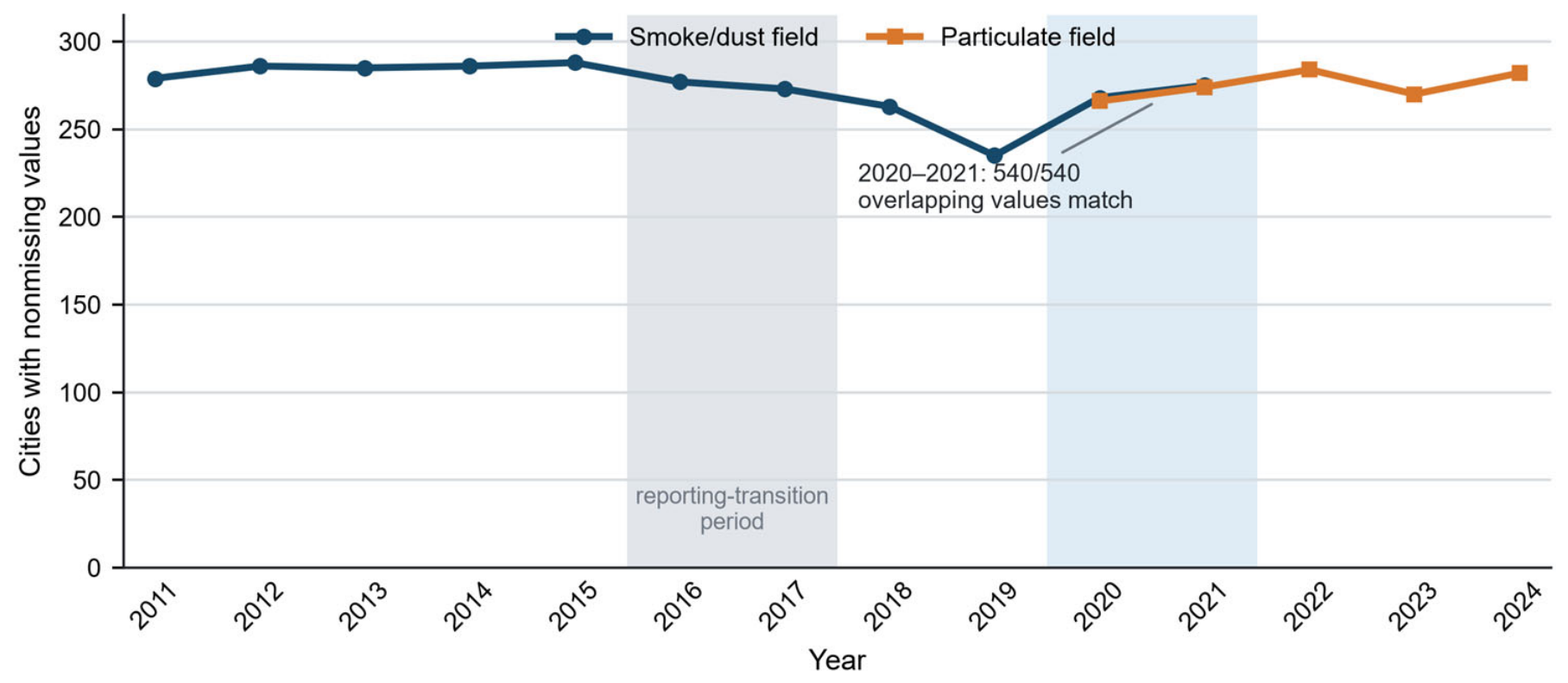
The database also contains a reported-series bridge. Smoke/dust and particulate-emission fields overlap in 540 city-years during 2020–2021, and all 540 values are identical. Official statistical materials define industrial soot/dust [61]. The second pollution-source census plan documents the transition [62]. The later bulletin records the reporting context [63]. Because levels and coverage also change around 2016–2017, the analysis treats these years as a documented reporting-transition period. The interaction remains similar when the transition years are omitted. Figure 5 summarizes annual field coverage and the overlap bridge.

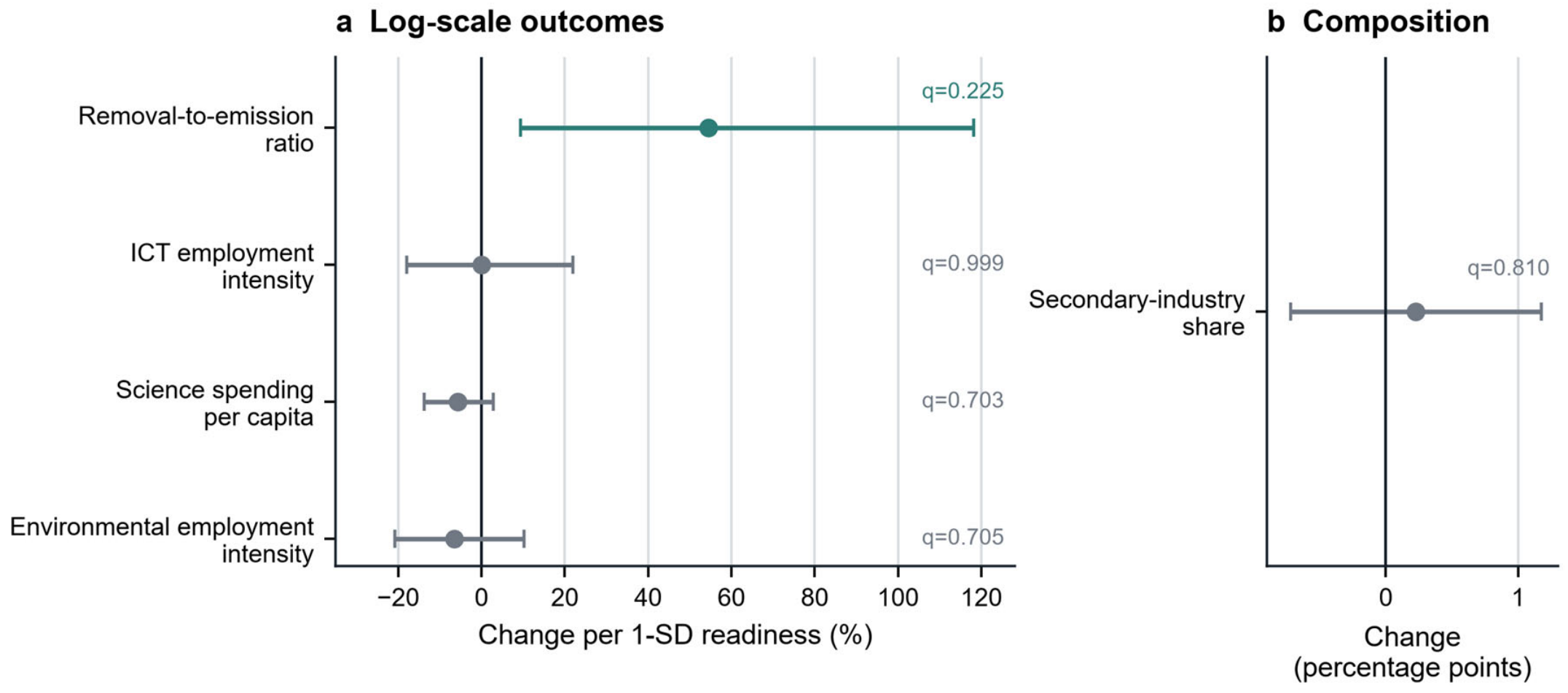
The mechanism family does not explain the gradient. The removal-to-emission ratio rises by 54.51% per standard deviation of readiness, but its adjusted q-value is 0.225 and all other estimates are imprecise. This is a directionally consistent signal, not a verified mediator. Figure 6 summarizes the mechanism-family estimates.

4.9. What Remains Supported

The diagnostics leave three empirically distinct results. The wastewater increase is precise before selection adjustment but attenuates afterward; the mobile-subscription elasticity is near zero over its prespecified grid; and the readiness interaction is negative but exploratory over limited support. These estimates answer different questions and should not be combined into a single environmental coefficient.

Table 8. Additional robustness, construct-boundary, and support diagnostics.

Domain	Diagnostic	Estimate or Range	95% Interval or Support	p-Value or Decision
Wastewater	Group-time aggregate	17.15%	8.58% to 26.59%	0.001
Wastewater	Cross-fitted doubly robust	7.69%	−2.09% to 18.43%	0.130
Wastewater	Leave-one-province estimates	16.45% to 22.77%	31 leave-one-province specifications	All positive
Mobile–PM2.5	Primary elasticity	0.0050	−0.0362 to 0.0461	0.813
Mobile–PM2.5	Prespecified 32-model grid	−0.020 to 0.059	9/32 negative; 4 nominal	0 FDR significant
Mobile–PM2.5	Equivalence bound ±0.05	—	Prespecified bound	0.016; supported
Mobile–PM2.5	Equivalence bound ±0.03	—	Prespecified bound	0.117; not supported
Readiness	Conditional contrast at −1 SD	31.48%	3.33% to 67.29%	0.0262
Readiness	Conditional contrast at mean	6.81%	−8.22% to 24.30%	0.3929
Readiness	Conditional contrast at +1 SD	−13.23%	−28.51% to 5.33%	0.1506
Readiness	Cohort-specific overlap support	Treated ESS: 25.89/21.72/20.52	Control ESS: 52.20/76.09/86.67	Max weight: 7.72/4.96/3.86

Note: Intervals are 95% confidence intervals. ESS denotes effective sample size; FDR, false-discovery rate; SD, standard deviation. Cohort-specific support values are ordered 2014/2015/2016. The rows summarize distinct estimands and should not be compared as if they measured one construct.

and Figure 7 and Figure 8 report the support, placebo, and construct-boundary diagnostics for these results. Together, they identify which comparisons remain descriptive, which are bounded by support, and which require independent confirmation.

5. Discussion

5.1. What the Evidence Establishes

The evidence establishes a boundary on interpretation rather than a universal policy coefficient. Official designation cannot stand in for realized network improvement when the physical-network first stage fails its declared gates. Likewise, reported source discharge, municipal services, river quality, and ambient PM_2.5 remain separate environmental objects. The readiness gradient adds a capacity-conditioned pattern but not a designation benefit for every city.

5.2. Why Prior Studies Can Disagree

The findings do not refute favorable digital-policy estimates. Prior studies examine pollution composites [1], air-quality indices and PM_2.5/GDP [2], PM_2.5 concentration [3], ecological welfare [4], and industrial-pollution indices [12]. Each measure remains useful at its stated level, but none can be translated automatically into a single physical-pollution response. Differences persist within air quality: PM_2.5/GDP measures intensity, whereas PM_2.5 alone measures concentration. A related Sustainability study links Broadband China to green total factor productivity and emphasizes local development conditions [64]. It supports attention to conditioning capacity but does not test portability across direct outcomes, denominators, weights, and observational units.

The analysis therefore defines an evidentiary boundary rather than a preferred average coefficient. The audit brings familiar first-stage, support, outcome, denominator, weighting, and multiplicity checks into one application; it should be read as an organizing procedure, not as a new causal estimator. The readiness gradient remains the least mature result and requires confirmation in an independent sample.

5.3. Mechanisms Remain Unresolved

The annual city data do not identify the mechanism behind the wastewater increase. Industrial wastewater rises, but sulfur dioxide is imprecise, municipal sewage changes little, and the balanced river estimate is also imprecise. The pattern could reflect production, industrial composition, physical discharge, reporting coverage, or several processes together. It does not establish that broadband increased total industrial activity or river pollution.

A monitoring explanation would require reported source discharge to diverge from a matched physical measure on common support. The available industrial, river, and PM_2.5 data do not provide that match. Policy attention, transparency scores, monitoring disclosure, and treatment-rate availability also fail to form a reliable chain. Testing this mechanism requires linked records on equipment, inspections, penalties, physical discharge, and ambient conditions.

5.4. Implications for Policy Evaluation

The findings imply a question-first rule for selecting policy indicators. Official designation is an appropriate measure of policy assignment, but it is not a proxy for completed infrastructure or service quality unless a credible implementation first stage is demonstrated. Ports and fiber measure physical supply; subscriptions and use measure adoption; and speed, latency, reliability, and effective coverage measure service quality. Future evaluations should name the stage they intend to estimate and verify expected-direction movement at that stage before interpreting designation as realized implementation.

Environmental indicators should likewise match the claim. Reported source discharge is appropriate for questions about regulated-source reporting or abatement; municipal sewage measures public service volume; ambient PM_2.5 measures receptor concentration; PM_2.5/GDP measures economic intensity; and a composite represents only its disclosed components and weighting rule. The present wastewater result does not transfer to ambient PM_2.5, while the denominator identity and weight surface show why intensity and composite results must be reported with their numerator, denominator, components, and weights.

A practical evaluation should therefore prespecify an indicator chain, retain component results, document coverage and definition changes, and compare alternatives in the same city-years before using separate data systems as external checks. Direct network-quality measures should be linked to source emissions, inspections, enforcement, and ambient records whenever possible. Baseline readiness can define monitoring strata and complementary investments, but the observed gradient is not an automatic targeting rule: low-readiness cities may need adoption, skills, and operating capacity, whereas high-readiness cities still require direct verification of network performance and environmental outcomes. An indicator that is not portable across designation, realized implementation, and outcome layers should therefore not be used alone to justify infrastructure funding, environmental targets, or cross-city performance comparisons.

5.5. Limitations and Evidence Needs

The principal limitation is identification. Designation was not random, observed-selection adjustment cannot remove unobserved time-varying confounding, and no physical-network measure passes every implementation gate. The estimates therefore describe designation rather than measured speed, reliability, or effective use. Outcome measurement creates additional limits: industrial records may mix physical and reporting changes; centroid weather omits within-city gradients; river estimates depend on station coverage and weights; and the weight simplex reveals sensitivity without defining a normatively correct index.

The readiness analysis is exploratory because it uses the same city database in which the signal was found. The smoke/dust series also has a 2016–2017 transition risk, and province-level mechanism tests are underpowered after multiplicity adjustment. Independent data on network quality, source emissions, monitoring, enforcement, and ambient conditions are needed to test whether the observed gradient replicates and why it arises.

6. Conclusions

The evidence is most clearly summarized as a sequence: designation, realized implementation, adoption, service quality, source outcomes, and ambient outcomes. In this application, the wastewater estimate, near-zero subscription elasticity, and readiness gradient are informative only for their named measures and observed support. Selection adjustment and multiplicity diagnostics further narrow the causal and mechanistic interpretation.

The paper does not propose a new causal estimator. Its contribution is to show, within one auditable application, how conclusions narrow when implementation, outcome, denominator, weighting, observational unit, and baseline capacity are aligned. Future work can test these boundaries by linking direct network-quality measures to source emissions, enforcement, and ambient monitoring in an independent setting.