The Role of Car Ownership in Sustainable Urban Transport: LRT Adoption in Kerman, Iran

Abstract

New Light Rail Transit (LRT) systems are frequently promoted as a means of reducing car dependence and supporting urban sustainability; however, their effectiveness depends on how different traveller segments respond to LRT relative to competing modes. This study examines whether car owners and non-car owners exhibit distinct preference structures and policy sensitivities towards a proposed LRT system in Kerman, Iran. A stated-preference mode-choice survey conducted in November 2023 generated 1916 valid choice observations, including 955 observations from car owners and 961 from non-car owners, based on 736 completed questionnaires. Multinomial Logit (MNL), Nested Logit (NL), and Mixed Logit (MXL) models were estimated separately for each segment. Policy implications were assessed using elasticities, marginal effects, and scenario-based simulations. The results show that, for car owners, the MXL specification provides a slightly better statistical fit, indicating modest preference heterogeneity, while the main behavioural conclusions remain consistent across model structures. For non-car owners, the NL model performs best, revealing clearer substitution between public-transport modes (bus/LRT) and on-demand services (taxi/ride-hailing). Although LRT shows a negative baseline preference, particularly among car owners, its uptake increases substantially with improved LRT travel-time performance and higher private-car operating costs. Overall, improving LRT travel-time competitiveness is critical for both groups, while attracting car owners additionally requires coordinated measures that raise the generalised cost of private-car use and strengthen the relative advantage of LRT. These findings highlight the importance of segment-sensitive policy design for maximising the contribution of LRT to sustainable urban transport and long-term urban sustainability.

1. Introduction

A persistent challenge for sustainable transport policy is that new urban rail investments do not automatically yield proportional reductions in private-car use. Although post-implementation evidence and synthesis studies generally indicate increases in rail mode share and reductions in car use and vehicle travel, these effects vary across settings and traveller groups [1]. This uncertainty is particularly important in car-oriented cities where LRT is expected to contribute not only to congestion mitigation and air-quality improvement, but also to longer-term shifts toward more sustainable urban mobility. In such contexts, understanding the conditions under which LRT becomes a credible substitute for private driving—rather than primarily redistributing demand within the public-transport market—remains a central policy concern.

Kerman provides a relevant empirical context for examining this issue. It is the capital of Kerman Province in south-eastern Iran and had a population of 537,718 in the 2016 national census [2]. Previous Kerman-based research has shown that car ownership and public-transport ridership are associated with socio-demographic characteristics and activity patterns, indicating that travel behaviour in the city is shaped by heterogeneous mobility needs and constraints [3]. In addition, a Kerman-based study on public-transport usage identified factors such as insufficient schedule information, limited passenger facilities, unsuitable waiting conditions, and perceived unreliability as barriers that can discourage public-transport ridership [4]. These local characteristics make Kerman a suitable pre-implementation setting for examining whether a proposed LRT system can compete with existing alternatives and influence traveller groups with different levels of car dependence. In this study, the LRT alternative is analysed as a pre-implementation stated-preference scenario rather than as an operating system. The analysis does not evaluate the technology choice between LRT and BRT; instead, it evaluates stated behavioural responses to the LRT alternative specified in the SP experiment. This pre-implementation context makes stated-preference analysis particularly appropriate, because it allows potential behavioural responses to be evaluated before irreversible infrastructure investments are made.

Evaluating such behavioural responses prior to implementation is inherently difficult because revealed-preference evidence is unavailable for services that are not yet operating and for policy packages that have not yet been enacted. In these settings, stated-preference (SP) experiments remain the principal tool for ex ante assessment, allowing systematic and controlled variation in key service attributes (e.g., travel time, access time, fare, reliability proxies) and identification of attribute trade-offs under ceteris paribus conditions [4,5,6]. SP approaches have been used extensively to assess emerging mobility options and their substitution patterns, and this literature consistently highlights that sensitivities to time and cost—and the resulting shifts across competing alternatives—can differ materially across user segments and baseline travel habits [7,8,9]. Consequently, segmentation is not an optional modelling refinement; it can be essential when policy success depends less on average responses and more on changing behaviour among specific target groups (notably current car users).

Within the LRT adoption literature, private-car ownership stands out as a particularly consequential source of heterogeneity. Car ownership is closely intertwined with habitual mode use, perceived convenience, and behavioural constraints that can shape willingness to adopt public transport—often in ways that are not well captured by treating ownership as merely another socio-demographic control [10]. Related evidence also shows that private-vehicle users and public-transport users can differ systematically in perceptions, satisfaction mechanisms, and behavioural intentions towards public transport, suggesting that the determinants of adoption and the leverage points for policy may not be symmetric across these groups [11,12,13]. At the same time, the SP evidence on LRT indicates that service-level attributes—especially time and fare—are consistently influential drivers of stated rail choice, while psychological and perceptual mechanisms such as a “rail bonus” can further differentiate rail from bus services even under comparable objective conditions [14,15]. More recent empirical evidence similarly suggests that rail services can carry an additional preference premium relative to comparable bus services, although the magnitude of this rail bonus is context-dependent [16]. In car-oriented contexts, targeted SP analyses focusing on car users further suggest that car-to-LRT switching is feasible, but conditional on clear performance advantages and supportive demand-management conditions (e.g., parking policy), reinforcing the view that attracting drivers requires a distinct policy logic rather than a generic “build-and-they-will-come” expectation [17]. More broadly, SP research on new mobility technologies has shown that designing experiments and models that explicitly distinguish owners from non-owners can reveal substantially different sensitivities and uptake propensities across these segments [18]. Taken together, these strands motivate the hypothesis that car owners and non-owners may exhibit not only different parameter magnitudes but potentially different preference regimes with distinct implications for LRT policy portfolios. Against this backdrop, the present study addresses two main research questions. First, how do car owners and non-car owners differ in their stated preferences for LRT relative to existing travel alternatives? Second, which service and policy-relevant factors most strongly influence predicted LRT uptake within each ownership segment, and what do these sensitivities imply for segment-specific LRT policy design? Model comparison across MNL, MXL, and NL specifications is treated as a methodological robustness check rather than as a separate research question. The preferred specification for each ownership segment is used for the primary behavioural interpretation, while alternative specifications are retained to examine whether the main policy implications are sensitive to different assumptions about substitution patterns and unobserved heterogeneity.

Based on these research questions, the study tests the following hypotheses:

H1. 

Car owners and non-car owners exhibit distinct preference structures towards the proposed LRT system and competing travel modes.

H2. 

Car owners are expected to show baseline resistance to LRT adoption, reflecting private-car availability, habitual car use, and the perceived convenience of private vehicles.

H3. 

LRT travel time negatively affects the probability of choosing LRT in both ownership segments, but its relative policy importance differs between car owners and non-car owners.

H4. 

Increases in the generalised cost of private-car use increase the probability of LRT adoption among car owners.

H5. 

For non-car owners, LRT substitution is expected to be structured primarily between fixed-route public-transport alternatives and flexible private-like motorised alternatives, implying stronger substitution between LRT and bus than between LRT and taxi/ride-hailing.

To answer these questions, the study employs an ownership-segmented SP design and estimates discrete choice models separately for car owners and non-car owners. MNL, MXL, and NL specifications are compared to identify the preferred behavioural representation for each segment and to assess the robustness of policy-facing results. This design enables direct comparison of behavioural regimes by ownership status and supports translation of model outputs into policy-relevant indicators such as scenario-based mode-share responses and sensitivity measures. The contribution is threefold: it provides ownership-segmented behavioural evidence on LRT adoption; it translates model outputs into policy-relevant indicators such as scenario-based mode-share responses and sensitivity measures; and it informs targeted, segment-specific LRT-based policy packages rather than generic one-size-fits-all recommendations. The remainder of the paper is organised as follows. Section 2 reviews the relevant literature on LRT impacts and pre-implementation adoption modelling. Section 3 describes the SP survey design, data, and modelling framework. Section 4 and Section 5 present estimation results and behavioural interpretation by ownership segment, followed by a robustness-oriented comparative analysis of policy indicators. Section 6 concludes with policy implications, limitations, and directions for future research.

2. Literature Review

Recent synthesis evidence reinforces this interpretation by showing that rail-transit interventions generally increase rail mode share and reduce bus share, car share, and vehicle miles travelled, although the magnitude of these effects varies across contexts [1]. Recent LRT ridership research further shows that accessibility, service quality, intermodal integration, station facilities, walking conditions, travel cost, and security are important determinants of urban rail demand [19]. For instance, the Metrolink in Greater Manchester significantly increased rail mode share, but with limited evidence of reduced car ownership, suggesting demand was largely drawn from former bus users [20,21]. In Cagliari, LRT attracts users valuing shorter travel times and less stress, with usage influenced by service performance and socio-demographic factors [22]. Evidence from Addis Ababa points to economic benefits like travel time/cost savings and improved job access, rather than large-scale reductions in car use [23,24]. In Los Angeles, proximity to a new LRT line reduced vehicle miles travelled and emissions, though effects diminished with distance from stations [25].

At a broader level, a recent systematic review and meta-analysis of natural experiments concludes that urban rail systems systematically increase rail mode share while reducing bus and car shares and vehicle miles travelled, though effect sizes and study quality vary considerably, highlighting the need for further research [1]. Complementing this, a thematic review of 53 LRT and metro ridership studies categorises determinants into six themes—land use and accessibility, service quality, user benefits, governance, sustainability, and user-focused attributes—emphasising the critical role of accessibility and intermodal connectivity [19]. This evidence underscores the context-dependent nature of LRT impacts and the importance of understanding who shifts travel modes and under what conditions. To predict travel behaviour before implementation, a growing number of studies employ stated-preference (SP) experiments. For a proposed LRT network in Flanders, in-vehicle time and fare were dominant factors, with waiting time, access/egress time, seat availability, and socio-economic characteristics also shaping preferences [14]. Recent first/last-mile evidence also shows that weak access between origins/destinations and transit stations can reduce public-transport patronage and increase the likelihood of direct car use, supporting the inclusion of access-related variables in LRT adoption models [26].

In Jakarta, fare was the most sensitive attribute, followed by travel and walking times [27]. Research in Addis Ababa found that the main predicted shift to LRT would come from existing bus users, not private-car drivers, with key factors including travel time, cost, and user demographics [28]. In Calgary, modelling of service disruptions showed ridership could drop by about one-third, with pass holders and frequent users more likely to remain loyal [29]. In Tehran, a 10% reduction in LRT travel time and better seat availability increased the likelihood of car users switching to LRT, while car ownership, frequent car use, free parking, and male gender reduced it [17]. Collectively, these pre-implementation studies highlight the strong influence of service-level attributes in hypothetical mode choices and the significant, context-dependent variation in user preferences. Recent evidence on emerging mobility services further shows that LRT adoption occurs within a wider substitution environment that includes ride-hailing, on-demand services, shared micromobility, and integrated mobility platforms. SP, RP/SP, and revealed-preference studies of ride-sourcing and transit-integrated ride-sourcing indicate that these services may either compete with public transport or complement it by improving access, depending on travel time, fare, transfer conditions, parking cost, trip purpose, and user characteristics. This evidence supports the explicit inclusion of taxi and ride-hailing alternatives in the present SP choice set [30,31,32].

Across this literature, three broad groups of determinants influencing Light Rail Transit (LRT) adoption are identified: traveller characteristics, mode attributes, and trip and spatial characteristics [19,33]. First, traveller characteristics demonstrate that socio-demographic and attitudinal variables significantly impact LRT usage. Studies from Flanders and Addis Ababa reveal that higher income and car ownership correlate with a lower stated preference for LRT [14,28]. Cagliari’s post-implementation study shows that younger individuals and those with prior bus experience are more likely to adopt LRT, while car owners use it less frequently [22]. In contexts like Addis Ababa, perceptions of benefits associated with LRT—such as reduced travel time and cost, improved accessibility, and satisfaction—vary with income, occupation, trip purpose, and usage frequency [23,24,34]. The second group, mode attributes, highlights critical factors driving LRT choice. Research consistently indicates that travel time, fare, reliability, and service frequency are core determinants [14,17,19,27,29,33]. Notably, studies show that additional waiting time poses a higher disutility than equivalent increases in-vehicle time [29], and fare is a highly sensitive attribute [27]. User perceptions also reveal that comfort, crowding, safety, information provision, and perceived stress influence satisfaction and willingness to use LRT [22,34]. The third group focuses on trip and spatial characteristics, revealing that LRT is more competitive for medium- to long-distance trips in congested corridors. The Flanders experiment showed LRT’s advantages grow as generalised cost differences increase for trips of 10–40 km [14]. Furthermore, supportive station-area conditions, such as higher density, mixed land use, and strong feeder/pedestrian links, are associated with higher ridership, though this relationship can be complex [23,24,35,36].

Private-car ownership provides a specialised theoretical basis for segmenting travellers into owners and non-owners. Recent developing-country evidence also supports this treatment of car ownership. In Dhaka, Ashik et al. show that car ownership mediates the relationship between the built environment, commute distance, and commute mode choice, highlighting its role as a structural behavioural factor rather than a simple demographic descriptor [37].

Rather than being a simple socio-demographic control, car ownership reflects vehicle availability, habitual mode use, perceived convenience, and different reference alternatives [10]. This is consistent with evidence that private-vehicle users and public-transport users differ in their perceptions of service quality, satisfaction, attitudes, and behavioural intentions towards public transport [11,12,13]. Accordingly, car owners may evaluate LRT relative to the flexibility, privacy, and door-to-door convenience of private vehicles, whereas non-car owners may compare LRT mainly with buses, taxis, and ride-hailing services. LRT-specific evidence supports this distinction. Studies in Flanders and Addis Ababa show that car ownership is associated with lower stated preference for LRT [14,28], and post-implementation evidence from Cagliari indicates lower LRT use among car owners [22]. Conversely, evidence from Tehran suggests that car-to-LRT switching is possible when LRT provides clear service advantages and supportive car-use conditions are considered [17]. Overall, these findings suggest that car owners and non-car owners may operate under structurally different preference regimes. However, much of the SP literature still relies on pooled models or treats ownership only as a covariate. This gap directly motivates the ownership-segmented modelling strategy adopted in this study.

3. Methodology

3.1. Data Collection and Survey Design

The survey was administered in Kerman, Iran, from 5 to 7 November 2023 to residents aged 18 and above. Two ownership-specific stated-preference (SP) questionnaires were developed for car owners and non-car owners. Each instrument covered: (i) socio-economic characteristics (e.g., age, gender, occupation, education, driving licence), (ii) the most recent trip (mode, purpose, start/end times), (iii) four SP choice scenarios based on travel time and cost (tailored by ownership group), and (iv) supplementary items on public-transport use and constraints (e.g., bus-use frequency, acceptable access/waiting times, and transfer tolerance). The design was informed by the literature and calibrated to local travel conditions. To improve the transparency of the stated-preference experiment,

Table 1. Choice sets, attributes, and task structure in the analysed stated-preference experiment.

Respondent Group	Analysed Choice Set	No. of Alternatives	No. of Tasks	Main Attributes	Design Rationale
Car owners	Car; taxi; bus; LRT; ride-hailing	5	4	Travel time; fare/cost; parking fee; fuel price	Includes private car as a competing option
Non-car owners	Taxi; bus; LRT; ride-hailing	4	4	Travel time; fare/cost	Excludes private car from the choice set

summarises the ownership-specific choice sets retained for analysis, the number of tasks, and the main attributes shown to respondents. Two questionnaire versions were prepared because car owners and non-car owners faced different feasible travel alternatives. In each SP task, respondents compared the available alternatives mainly in terms of travel time and monetary cost/fare, and then indicated their preferred alternative. For car owners, the analysed choice set included private car, taxi, bus, the proposed LRT alternative, and app-based taxi/ride-hailing. For non-car owners, the private-car alternative was excluded, while the remaining alternatives followed the same task structure. This design allowed LRT to be evaluated against the alternatives that were behaviourally relevant to each ownership group.

The attribute levels were selected to represent realistic differences in travel time and monetary cost among the available and proposed alternatives in Kerman. The levels were anchored to respondents’ current trip conditions, the expected operational characteristics of the proposed LRT system, and values commonly used in previous LRT stated-preference studies. For each ownership group, the levels were calibrated so that LRT was evaluated against behaviourally relevant alternatives rather than unrealistic or unavailable options. This ownership-specific calibration ensured that the SP tasks reflected plausible trade-offs faced by car owners and non-car owners in the Kerman context. A structured scenario-based SP design was used. The design systematically varied the main policy-relevant attributes, particularly travel time and monetary cost, while keeping the number of choice tasks manageable for respondents. Implausible or clearly dominated alternatives were avoided during scenario construction to ensure that respondents faced meaningful time-cost trade-offs rather than obvious choices. Each respondent evaluated four SP tasks, which provided repeated observations for model estimation while limiting cognitive burden.

To further clarify the SP experiment,

Table 2. SP choice tasks retained for analysis: car-owner questionnaire.

Task	Car	Taxi	Bus	LRT	Ride-Hailing
1	15 min; parking fee: 5000; fuel price: 3500/litre	20 min; fare: 6000	40 min; fare: 1500	35 min; fare: 500	15 min; fare: 25,000
2	15 min; parking fee: 7000; fuel price: 5000/litre	20 min; fare: 8000	30 min; fare: 2000	20 min; fare: 700	15 min; fare: 35,000
3	15 min; parking fee: 10,000; fuel price: 7000/litre	20 min; fare: 10,000	40 min; fare: 2500	25 min; fare: 1000	15 min; fare: 45,000
4	60 min; parking fee: 1000; fuel price: 2500/litre	25 min; fare: 8000	35 min; fare: 2000	25 min; fare: 500	20 min; fare: 25,000

and

Table 3. SP choice tasks retained for analysis: non-car owner questionnaire.

Task	Taxi	Bus	LRT	Ride-Hailing
1	20 min; fare: 6000	40 min; fare: 1500	35 min; fare: 500	15 min; fare: 25,000
2	20 min; fare: 8000	30 min; fare: 2000	20 min; fare: 700	15 min; fare: 35,000
3	20 min; fare: 10,000	40 min; fare: 2500	25 min; fare: 1000	15 min; fare: 45,000
4	25 min; fare: 8000	35 min; fare: 2000	25 min; fare: 500	20 min; fare: 25,000

report the four choice tasks retained for analysis for car owners and non-car owners, respectively. Rather than presenting only one illustrative example, these tables report all retained SP tasks used in the final modelling dataset. They show the alternatives, travel-time levels, and monetary cost/fare levels presented to respondents in each task. Monetary values are reported in Tomans, consistent with the original questionnaire cards. For comparability with other monetary values reported elsewhere in the paper, approximate USD equivalents were calculated using a rounded exchange rate of 1 USD = 50,000 Tomans (500,000 IRR), corresponding to the November 2023 survey period.

These tables show that the SP tasks varied both travel time and monetary cost/fare across alternatives. For car owners, the private-car option was included to capture direct competition between LRT and private driving. For non-car owners, the same task logic was used, but the private-car option was excluded because it was not a feasible ownership-based alternative.

A pilot survey involving 60 participants, including 30 transportation engineering graduate students and 30 lay participants, was conducted before the main survey. The pilot was used to assess questionnaire clarity, scenario plausibility, the comprehensibility of attribute levels, and the feasibility of completing four SP tasks without excessive respondent burden. Internal consistency was assessed for the repeated LRT choice indicators across the four SP tasks, because LRT adoption is the focal behavioural outcome of the study. Internal consistency was assessed for the SP block using the four repeated LRT choice indicators. For the pooled pilot sample across the car-owner and non-car owner questionnaire versions, Cronbach’s alpha was 0.926, indicating the very good internal consistency of the SP block. Because these four LRT indicators are binary repeated-choice indicators rather than Likert-type scale items, Cronbach’s alpha is used here only as an exploratory internal-consistency check for the SP block. Pilot responses were also screened for missing values, inconsistent responses, and implausible scenario evaluations. Face validity was assessed through expert review and participant feedback, and minor wording and formatting revisions were made before the main survey.

The main survey was conducted through interviewer-administered questionnaires at 12 strategically selected urban locations using a systematic intercept sampling procedure. The survey locations were selected to cover major urban activity and travel-generation points in Kerman, including areas with different public-transport access conditions and trip purposes. At each location, trained interviewers approached every tenth eligible passer-by aged 18 years and above during the survey period. If the selected person declined to participate or was not eligible, the interviewer proceeded to the next tenth eligible passer-by. Respondents were first screened for car-ownership status and then assigned to the corresponding questionnaire version. This procedure was designed to obtain a diverse sample of urban travellers at selected activity locations rather than a fully random household sample of all Kerman residents.

Of 820 completed interviews, 736 respondents remained after respondent-level data cleaning, including 388 car owners and 348 non-car owners. Thus, 84 questionnaires were excluded at the respondent level because they contained incomplete socio-demographic or trip information required for segmentation, incomplete SP responses, or insufficient usable information for subsequent choice modelling. Each respondent encountered four SP choice scenarios, leading to a potential total of 2944 SP choice observations. After choice-observation-level screening, 1916 valid SP observations were retained for model estimation, including 955 from car owners and 961 from non-car owners. To clarify the data-screening process,

Table 4. Respondent screening and retained SP choice observations.

Item	Car Owners	Non-Car Owners	Total
Completed interviews	—	—	820
Valid respondents after respondent-level screening	388	348	736
Potential SP choice observations	1552	1392	2944
Retained valid SP observations	955	961	1916
Dropped SP observations	597	431	1028
Retention rate	61.5%	69.0%	65.1%

summarises the transition from completed interviews to the final respondent sample and the retained SP choice observations used for model estimation.

At the choice-observation level, invalid SP tasks were removed only when the task was incomplete, when the selected alternative was missing, or when more than one alternative was selected in the same choice task, making the dependent variable ambiguous. The latter case is what is meant here by a scenario-specific inconsistency. No additional behavioural exclusion rule, such as speed-based rejection, straight-lining, or dominated-alternative violation, was applied at the choice-observation level. Of the 1028 dropped SP observations, 875 were excluded because of incomplete SP tasks or missing selected alternatives, while 153 were excluded because multiple alternatives were selected in the same task. Because invalid tasks were removed at the task level rather than deleting all observations from the corresponding respondent whenever possible, respondents could contribute between one and four valid SP tasks. The final estimation dataset is therefore an unbalanced repeated-choice dataset. In the car-owner sample, respondents contributed one, two, three, and four valid tasks in 106, 124, 31, and 127 cases, respectively. In the non-car owner sample, the corresponding numbers were 57, 97, 66, and 128 respondents.

The adequacy of the sample size for the ownership-specific choice-modelling task is supported by several methodological and statistical considerations. First, the minimum sample-size requirement was checked using Orme’s rule of thumb for stated-preference investigations:

$$N>{\displaystyle \frac{500\times c}{t\times a}}$$

(1)

where N denotes the minimum required sample size, c denotes the number of alternatives, t denotes the number of choice tasks per respondent, and a denotes the maximum number of attribute levels. In the present study, c = 5 for car owners and c = 4 for non-car owners, t = 4, and a = 4, yielding minimum required sample sizes of 157 for car owners and 125 for non-car owners. These values are well below the retained respondent samples of 388 car owners and 348 non-car owners. Second, the econometric complexity of the employed Nested Logit (NL) and Mixed Logit (MXL) models necessitates a richer dataset than simple logit models, given the need to estimate random-parameter distributions and correlation structures. The provision of approximately 1000 observations per ownership segment (car owners versus non-owners) supplies sufficient degrees of freedom to achieve conventional levels of statistical significance for the majority of covariates. Third, as a survey-size check, the final sample of 736 respondents exceeds the commonly cited minimum sample size of approximately 384 respondents for large populations under a 95% confidence level and 5% margin of error, assuming maximum variability (p = 0.5) [38]. Using the same conservative assumption and applying the finite-population margin-of-error expression from Cochran [38] to an approximate city population of 750,000 gives an indicative margin of error of about 3.6% for the respondent sample. This calculation should be interpreted as a sampling-precision check rather than as a claim of full demographic representativeness, since the survey was conducted at selected urban locations. The indicative margin of error was computed as Equation (2):

$$e=Z\sqrt{\left({\displaystyle \frac{p(1-p)}{n}}\right)\left({\displaystyle \frac{N-n}{N-1}}\right)}$$

(2)

where Z = 1.96 for a 95% confidence level, p = 0.5, n = 736, and N ≈ 750,000.

Fourth, the segmentation strategy preserves analytical robustness after stratification; each subgroup retains roughly 370 respondents (≈950–960 observations), which is adequate to support rigorous comparative inference without incurring excessive stochastic variability. Finally, the estimation results, including the reported pseudo-R² values and likelihood-ratio statistics, suggest that the retained data contain sufficient information to estimate the ownership-specific choice models and capture relevant passenger behaviour patterns.

3.2. Model Specification and Variable Definition

The analytical framework of this study is grounded in Random Utility Theory (RUT) [4], which posits that individuals choose the alternative that maximises their perceived utility. The utility U_nj that individual n derives from choosing travel mode j is composed of a deterministic component V_nj and a stochastic error term ε_nj (Equation (3)).

$$U_{nj}=V_{nj}+{\epsilon }_{nj}$$

(3)

The deterministic component V_nj is specified as a linear function of observed attributes X_nj (e.g., travel time, cost, and socio-demographic interactions) with corresponding parameters β to be estimated. To robustly analyse mode-choice behaviour towards the hypothetical Light Rail Transit (LRT) system and to explicitly test for structural differences between car owners and non-car owners, we estimate and compare three discrete choice model specifications separately for each group. The MNL, MXL, and NL models were estimated using PythonBiogeme version 3.2.14 (EPFL, Lausanne, Switzerland).

Socio-economic and trip-related variables were included in the utility functions only when they had a clear behavioural interpretation and improved model interpretability. Their inclusion was guided by the literature, local travel conditions, and theoretical expectations regarding access constraints, service familiarity, transfer tolerance, expenditure-based affordability, and mobility limitations. To reduce overfitting concerns, variables with weak behavioural justification or unstable signs were not retained in the final specifications.

In all estimated models, the dependent variable is the chosen alternative in each SP choice task. For car owners, the choice variable takes one of five alternatives: private car, taxi, bus, LRT, and ride-hailing. For non-car owners, it takes one of four alternatives: taxi, bus, LRT, and ride-hailing. The independent variables consist of alternative-specific service attributes, mainly travel time and monetary cost/fare, and selected socio-economic or trip-related interaction variables. Economic-status variables used in the models are based on the monthly household expenditure categories reported in

Table 5. Socio-demographic characteristics of respondents by car ownership status.

Characteristics	Frequency
	Car Owners		Non-Car Owners		Total
	Absolute	Relative (%)	Absolute	Relative (%)	Absolute	Relative (%)
Gender
Male	258	66	156	45	414	56
Female	130	34	192	55	322	44
Age
18–24	66	17	122	35	188	26
25–34	97	25	81	23	178	24
35–44	84	22	65	19	149	20
45–54	86	22	44	13	130	18
55–64	32	8	19	5	51	7
Over 65	23	6	17	5	40	5
Education
Illiterate	6	2	19	5	25	3
Less than high school diploma	53	14	57	16	110	15
High school diploma or associate degree	186	48	186	53	372	51
Bachelor’s degree	101	26	76	22	177	24
Master’s or PhD degree	42	11	10	3	52	7
Average monthly household expenditure
Low (<70 million IRR; <$140)	114	29	198	57	312	42
Lower-middle (70–120 million IRR; $140–$240)	154	40	90	26	244	33
Upper-middle (120–160 million IRR; $240–$320)	73	19	50	14	123	17
High (>160 million IRR; >$320)	47	12	10	3	57	8

Note: USD values are approximate and were calculated using an exchange rate of 1 USD = 50,000 Tomans (500,000 IRR), corresponding to the November 2023 survey period.

. The expenditure dummies are interpreted relative to the omitted reference category and should not be read as separate income variables. The exact variables included in each utility function are reported in the parameter-estimation tables. Blank cells in these tables indicate that the corresponding variable was not retained in that specification. Thus, the three model structures differ mainly in their behavioural assumptions—IID substitution in MNL, random taste heterogeneity in MXL, and within-nest correlation in NL—rather than in the definition of the dependent variable. Accordingly, coefficient-level comparisons are made primarily between MNL and MXL specifications, which share the closest utility structure. NL results are interpreted mainly as supplementary evidence on structured substitution, rather than as coefficient-by-coefficient replications of the MNL/MXL specifications.

3.2.1. Multinomial Logit Model

The MNL model serves as the baseline, assuming the error terms ε_nj are independently and identically distributed (IID) following a Gumbel distribution. This leads to the well-known closed-form probability expression shown in Equation (4):

$$P_{nj}={\displaystyle \frac{e^{V_{nj}}}{{\sum }_{k=1}^J{e}^{V_{nk}}}}$$

(4)

While computationally efficient, the MNL model imposes the Independence of Irrelevant Alternatives (IIA) property, which may be restrictive if certain modes are perceived as closer substitutes [6].

3.2.2. Mixed Logit Model

To account for unobserved preference heterogeneity across individuals, we employ a Mixed Logit model (also known as Random Parameters Logit). This flexible model allows parameters to vary randomly across the population [5]. The utility function in the MXL specification (Equation (5)) modifies the basic RUT framework:

$$U_{nj}={\beta }_n^{\prime }{\mathrm{X}}_{nj}+{\epsilon }_{nj}$$

(5)

where β_n is a vector of individual-specific parameters with density f(β_θ). The unconditional choice probability is the integral of the conditional logit probability over this distribution, as given by Equation (6):

$$P_{nj}=\int {\displaystyle \frac{e^{{\beta }^{\prime }{X}_{nj}}}{ {\displaystyle {\sum }_{k=1}^J}{e}^{{\beta }^{\prime }{X}_{nk}}}}f\left(\beta ∣\theta \right)d\beta$$

(6)

We estimate this probability using simulated maximum likelihood with 2000 Halton draws, following Train [6]; stability was checked by comparing alternative draw settings during model development. Because each respondent could contribute more than one valid SP task and the final dataset was unbalanced, respondent-level panel MXL specifications were also estimated as a diagnostic check using the available number of valid tasks per respondent. These panel estimations explicitly accounted for repeated-choice correlation within respondents and confirmed that the substantive behavioural conclusions were not sensitive to treating the retained SP tasks as an unbalanced repeated-choice dataset. In both ownership segments, the signs and substantive interpretation of the key policy-relevant effects remained unchanged, including the negative effect of LRT travel time, the role of private-car operating cost among car owners, and the main public-transport substitution mechanisms among non-car owners. For this reason, the panel MXL results are used as a diagnostic robustness check rather than reported as additional main specifications.

Candidate random parameters were retained only when the estimated heterogeneity was statistically meaningful, behaviourally interpretable, stable, and did not imply implausible sign reversal for time or cost coefficients. Random coefficients with negligible, unstable, or behaviourally implausible spreads were treated as fixed effects in the final MXL specifications. For the car-owner sample, the retained random parameters mainly capture heterogeneity in selected competing-mode travel-time sensitivities. For the non-car owner sample, the retained random parameters capture heterogeneity in bus schedule-related sensitivity and LRT travel-time sensitivity. A constrained triangular distribution was used for retained random parameters because it allows limited preference heterogeneity to be represented while preserving behaviourally interpretable coefficient signs.

3.2.3. Nested Logit Model

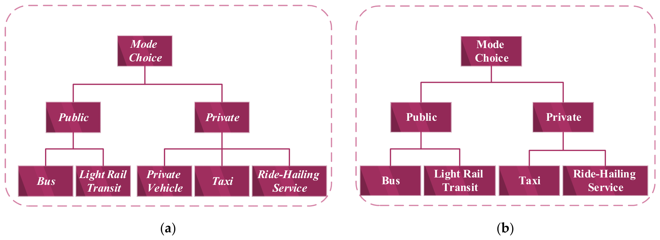
To relax the IIA assumption and to model potential correlation among similar alternatives, we test a two-level Nested Logit structure [6,39]. Given the distinct choice sets for car owners and non-car owners (Figure 1), we specify separate nesting structures for each group, reflecting their different available alternatives and potential substitution patterns:

• For car owners (Figure 1a), the tested nesting structure groups private-like motorised alternatives, namely private vehicle, taxi, and ride-hailing, separately from fixed-route public-transport alternatives, namely bus and LRT. This structure reflects the behavioural distinction between flexible, door-to-door or semi-door-to-door motorised modes and scheduled collective transport modes. This grouping does not imply that private car, taxi, and ride-hailing are behaviourally identical. Rather, in the Kerman context, where existing public transport faces limitations in service quality, reliability, passenger facilities, and information provision, these alternatives may be perceived as sharing unobserved attributes related to flexibility, reduced dependence on fixed schedules, and greater perceived individual control relative to conventional public transport. An alternative three-nest car-owner structure separating private car from hired/on-demand motorised services, namely {private car}, {taxi, ride-hailing}, and {bus, LRT}, was also tested. However, the singleton private-car nest produced unstable inclusive-value estimates and, in an alternative run, a singular variance–covariance matrix. Therefore, this alternative structure was not retained.
• For non-car owners (Figure 1b), the tested nesting structure groups taxi and ride-hailing as private-like motorised alternatives, while bus and LRT are grouped as fixed-route public-transport alternatives. This structure reflects the expectation that non-car owners compare LRT mainly with existing public transport on the one hand and flexible paid motorised services on the other.

In the NL model, the probability of individual n choosing alternative j in nest m is given by the product of a conditional and a marginal probability (Equation (7)):

$$P_{nj}=P_{nj\mid \mathrm{m}}.P_{nm}$$

(7)

where the conditional probability of choosing $j$ given nest $m$ is expressed in Equation (8):

$$P_{nj\mid m}={\displaystyle \frac{e^{V_{nj}/{\lambda }_m}}{{\sum }_{k\in B_m} e^{V_{nk}/{\lambda }_m}}}$$

(8)

and the marginal probability of choosing nest $m$ is given by Equation (9):

$$P_{nm}={\displaystyle \frac{e^{{\lambda }_m{I}_{nm}}}{{\displaystyle {\sum }_{l=1}^M} e^{{\lambda }_l{I}_{nl}}}}, \mathrm{with}{I}_{nm}=\mathrm{l}\mathrm{n}{\sum }_{k\in B_m}{e}^{V_{nk}/{\lambda }_m}$$

(9)

Nest-level covariates enter the marginal nest utility component of the NL model and affect the marginal probability of selecting nest m. They are not part of the inclusive-value/log-sum term itself, which is computed from the conditional utilities of alternatives within each nest. The inclusive-value parameter separately captures the degree of within-nest correlation. The inclusive-value (IV) parameter, ${\lambda }_m$, measures the degree of independence within the nest $m$. A value between 0 and 1 indicates that the nested structure is consistent with utility maximisation and that alternatives within the same nest are perceived as closer substitutes [39].

4. Results

4.1. Frequency Analysis

Table 5 presents the socio-demographic characteristics of the respondents by car ownership status. The results indicate a gender imbalance, with a substantially higher proportion of males among car owners (66%) than non-owners (45%). Non-car owners were predominantly younger (35% aged 18–24), whereas car owners exhibited a more balanced age distribution across the prime working ages (25 to 54). Although educational attainment was relatively high in both groups, advanced degrees (Master’s/PhD) were more prevalent among car owners (11%) than non-owners (3%), suggesting a link between higher education and the economic means for car ownership. Household expenditure patterns also revealed clear disparities: a majority of non-owners (57%) fell into the lowest monthly expenditure category, while car owners were concentrated in the lower-middle expenditure bracket and accounted for most high-expenditure households (12% vs. 3%). Overall, these systematic differences—consistent with theoretical expectations—justify analysing the mode-choice behaviour of the two groups separately.

Household economic status was represented by average monthly household expenditure rather than directly reported income. The objective was to construct a reliable proxy for household economic status, since direct income questions in field surveys may generate inaccurate or incomplete responses due to non-response, under-reporting, over-reporting, or reluctance to disclose. This issue is particularly relevant in high-inflation contexts, where nominal income may be unstable and difficult for respondents to report precisely. Monthly household expenditure was therefore used as a practical indicator of household economic status in the present survey.

4.2. Estimation Results for Car Owners

4.2.1. Model Comparison and Goodness-of-Fit Assessment—Car Owners

Table 6. Goodness-of-fit statistics for MNL, MXL and NL models—car owners.

No.	Statistic	Description	MNL	MXL	NL
1	LL(B)	Log-likelihood at convergence	−1256.860	−1256.102	−1275.288
2	LL(C)	Log-likelihood of Constant-only model	−1350.588	−1350.588	−1350.588
3	LL(0)	Log-likelihood of Null model	−1537.013	−1537.013	−1537.013
4	${\mathsf{\rho }}_0^2$	McFadden’s pseudo R2	0.182	0.183	0.17
5	${\mathsf{\rho }}_{\mathrm{c}}^2$	Pseudo R2 relative to constants	0.069	0.07	0.056
6	AIC	Akaike Information Criterion	2557.72	2556.204	2596.576
7	BIC	Bayesian Information Criterion	2664.678	2663.161	2708.395
8	K	Number of estimated parameters	22	22	23
9	N	Sample size	955	955	955

Note: LL(0) is computed consistently across all three specifications using the equal-probability null model over the five alternatives in the car-owner choice set.

presents the goodness-of-fit statistics for the three specifications estimated for the car-owner segment. The MXL model provides a slight improvement over the MNL benchmark in terms of log-likelihood and information criteria. Specifically, the log-likelihood improves from −1256.860 in the MNL model to −1256.102 in the MXL model, while AIC and BIC decrease from 2557.720 and 2664.678 to 2556.204 and 2663.161, respectively. This indicates that allowing for unobserved heterogeneity in travel-time sensitivity improves statistical fit, although the magnitude of the improvement is small.

The NL model does not improve the overall goodness of fit for the car-owner segment. It has a lower log-likelihood at convergence, LL(β) = −1275.288, and higher information criteria, AIC = 2596.576 and BIC = 2708.395, than both the MNL and MXL specifications. Therefore, the nested structure is not adopted as the primary model for the car-owner segment. Given the small difference between MNL and MXL and the consistency of their main behavioural conclusions, the MNL model is retained as the primary interpretive benchmark for the car-owner segment because of its parsimony, transparency, and straightforward behavioural interpretation. This supplementary status is also supported by the alternative nesting test, in which separating private car into a singleton nest did not yield a statistically stable NL specification. Thus, the subsequent interpretation focuses primarily on the MNL results, with MXL and NL results used as complementary evidence. For this segment, robustness is therefore assessed mainly through the stability of substantive mechanisms across specifications, not through coefficient-by-coefficient equality across different model structures. During the specification-development stage, LRT fare/cost was also examined in alternative car-owner MNL and MXL specifications because of its policy relevance. In these specifications, the LRT fare/cost coefficient had the expected negative sign but was not statistically significant. Specifically, the coefficient was −0.00046 in the fare-inclusive MNL specification and −0.00090 in the fare-inclusive MXL specification. By contrast, the coefficient was negative and statistically significant in the NL specification. Therefore, fare sensitivity for car owners is interpreted only as a supplementary, structure-dependent result, while the primary car-owner interpretation remains based on the more stable effects of LRT travel time and private-car operating cost. Accordingly, NL-based car-owner fare results are not used for primary model selection or as model-general policy forecasts; they are reported only to document a supplementary sensitivity mechanism that appears under the structure-dependent NL specification.

4.2.2. Interpretation of Key Parameter Estimates—Car Owners

Table 7. Parameter estimates for the MNL, MXL, and NL models—car owners.

Mode	Variable Symbol	Variable Definition	MNL	MXL		NL
			Parameter	Parameter	Std. Dev. (Triangular)	Parameter
Private Vehicle	FUEL_PRC	Fuel price	−0.176 *** (−6.88)	−0.198 *** (−6.26)	-	−0.263 ** (−2.20)
	CHL_0	Max acceptable bus transfers = 0 (1 = yes)	0.349 ** (2.17)	0.376 ** (2.23)	-	0.493 *** (2.86)
	HIGH_EXP	High expenditure (1 = yes)	0.925 *** (4.20)	0.937 *** (4.10)	-	0.940 *** (3.74)
	M_CAR	Last trip mode: private car (1 = yes)	0.337 ** (2.10)	0.333 ** (1.99)	-	-
	AGE_OV65	Age > 65 (1 = yes)	−0.710 ** (−2.17)	−0.753 ** (−2.21)	-	-
Taxi	T_CST	Travel Cost	-	-	-	−0.200 *** (−2.73)
	T_TME	Travel Time	−0.107 *** (−8.22)	−0.134 *** (−6.32)	0.127 *** (6.32)	-
	LOW_MED_EXP	Low–medium expenditure (1 = yes)	-	-	-	-
	TP_BSN (Male)	Last trip purpose: business & male (1 = yes)	−0.647 ** (−2.53)	−0.729 *** (−2.60)	-	−0.929 *** (−3.59)
	UP_MED_EXP	Upper-middle expenditure (1 = yes)	−0.751 ** (−2.39)	−0.816 ** (−2.37)	-	−0.793 ** (−2.53)
Bus	T_TME	Travel Time	−0.068 *** (−9.14)	−0.087 *** (−6.67)	0.083 *** (6.67)	−0.115 *** (−3.71)
	M_Walk	Last trip mode: walking (1 = yes)	0.804 ** (2.12)	1.049 ** (2.10)	-	1.393 *** (2.60)
	LOW_EXP	Low expenditure (1 = yes)	0.588 *** (3.19)	0.733 *** (3.09)	-	0.829 *** (3.26)
	AGE_OV65 (Male)	Male passenger age > 65 (1 = yes)	0.808 ** (2.10)	1.020 ** (2.10)	-	-
Light Rail Transit	ASC	Alternative-Specific Constant	−2.148 *** (−3.67)	−2.503 *** (−3.81)	-	-
	T_CST	Travel Cost	-	-	-	−0.961 *** (−2.95)
	T_TME	Travel Time	−0.051 *** (−2.94)	−0.047 ** (−2.57)	0.005 ** (2.57)	−0.103 *** (−3.41)
	OC_RTD	Retired occupation (1 = yes)	1.210 *** (4.31)	1.225 *** (4.22)	-	-
	CHL_3	Max acceptable bus transfers = 3 (1 = yes)	-	-	-	1.441 ** (2.14)
	A_SCH	Aware of schedule (1 = yes)	0.593 *** (2.64)	0.620 *** (2.71)	-	-
	WK_M	Max acceptable walking time to bus stop	0.068 *** (4.13)	0.069 *** (4.10)	-	-
	AGE_3544	Age 35–44 (1 = yes)	0.720 *** (3.10)	0.744 *** (3.15)	-	-
Ride-Hailing Service	T_TME	Travel Time	−0.074 *** (−3.07)	−0.075 *** (−3.07)	-	−0.067 *** (−2.75)
	T_CST	Travel Cost	−0.023 *** (−3.67)	−0.026 *** (−3.81)	-	−0.040 ** (−2.17)
	AGE_OV65	Age > 65 (1 = yes)	-	-	-	-
	MED_HI_EXP	Medium–high expenditure (1 = yes)	−0.879 ** (−2.52)	−0.896 ** (−2.55)	-	-
	M_TXI	Last trip mode: Taxi (1 = yes)	0.881 ** (2.39)	0.855 ** (2.28)	-	1.013 *** (2.72)

Note: Blank cells indicate variables not retained in the corresponding final specification. MNL and MXL provide the main basis for coefficient-level comparison, whereas NL is interpreted as a supplementary structure-dependent specification. ***, ** indicate significance at the 1%, 5% levels, respectively.

reports parameter estimates for the MNL, MXL, and NL models for the car-owner sample. Although the MXL model provides a slightly better statistical fit, the improvement over the MNL benchmark is small and the main behavioural conclusions remain consistent across specifications. Therefore, the MNL model is retained as the primary interpretive benchmark because of its parsimony, transparency, and straightforward behavioural interpretation, while the MXL model is used to assess unobserved preference heterogeneity and the NL model is used as a supplementary robustness specification for substitution patterns. Under the MNL specification, private-vehicle utility exhibits a statistically significant negative response to fuel price (FUEL_PRC = −0.176 ***), implying that higher private-car operating costs reduce the attractiveness of driving. Car use is more likely among respondents in the high household expenditure group (HIGH_EXP = 0.925 ***) and among those with zero tolerance for bus transfers (CHL_0 = 0.349 **), which is consistent with a preference for private travel when transfer inconvenience is unacceptable. Prior car use is also associated with higher current utility (M_CAR = 0.337 **), whereas respondents aged over 65 show lower private-vehicle utility (AGE_OV65 = −0.711 **).

For LRT, the alternative-specific constant is negative and statistically significant (ASC = −2.148 ***), indicating a lower baseline preference for LRT among car owners after controlling for observed attributes. LRT travel time is also negatively valued (T_TME = −0.052 ***), confirming the importance of travel-time competitiveness. However, LRT utility increases with retirement status (OC_RTD = 1.210 ***), schedule awareness (A_SCH = 0.593 ***), and greater walking-time tolerance to access public transport (WK_M = 0.068 ***). These variables were included in the LRT utility because they represent plausible behavioural mechanisms affecting LRT adoption among car owners, including lower driving burden among retirees, the importance of service information, and willingness to tolerate station-access walking.

Table 8. Nested Logit nest parameters—car owners.

Nest/Parameter	Variable	Definition	Parameter (t-Stat)
Private-Like Modes Nest	TP_MANF	Mandatory last trip purpose (1 = yes)	0.340 ** (2.18)
	AGE_5564	Age 55–64 (1 = yes)	0.838 *** (2.70)
	OC_RTDF	Retired male passenger (1 = yes)	0.686 *** (2.68)
Public-Transport Nest	WK_M	Max acceptable walking time to the bus stop	0.040 *** (2.92)
	AGE_1824	Age 18–24 (1 = yes)	−0.435 ** (−2.12)
	AGE_2534	Age 25–34 (1 = yes)	0.603 ** (3.13)
Inclusive-Value (IV) Parameters	λ_Private-like	IV (Private-like nest)	0.736 ** (2.07)
	λ_Public	IV (Public-Transport nest)	0.621 *** (3.16)

Note: ***, ** indicate significance at the 1%, 5% levels, respectively.

reports the NL-specific inclusive-value parameters. The inclusive-value point estimates are statistically significant and lie within the admissible range (λ_Private-like = 0.736 **; λ_Public = 0.621 ***), indicating that the tested nesting structure is behaviourally admissible. However, post-estimation Wald-type tests against unity indicate that λ_Public is only marginally different from 1 (z ≈ −1.93, p ≈ 0.054), whereas λ_Private-like is not statistically different from 1 (z ≈ −0.74, p ≈ 0.46). Therefore, the IV estimates alone do not establish the superiority of NL over MNL/MXL. Because the NL specification also does not improve overall fit relative to the MNL and MXL specifications in terms of log-likelihood and information criteria, the car-owner NL results are interpreted only as supplementary evidence on structure-dependent substitution and fare sensitivity. They are not used as the primary basis for coefficient interpretation or model-general policy simulation.

4.2.3. Derived Policy Indicators: Elasticities and Marginal Effects—Car Owners

Table 9. Discrete marginal effects (direct and cross) on LRT choice probability (car owners).

Mode	Variable	MNL	MXL	NL
Private Vehicle	CHL_0	−1.95	−2.17	−2.109
	HIGH_EXP	−5.16	−5.15	−4.098
	M_CAR	−1.84	−1.90	-
	AGE_OV65	3.75	4.23	-
Taxi	TP_BSN (Male)	1.05	1.17	0.977
	UP_MED_EXP	2.15	2.48	0.83
Bus	M_Walk	−2.46	−2.67	−6.47
	LOW_EXP	−1.58	−1.75	−3.91
	AGE_OV65 (Male)	−2.44	−2.65	-
Light Rail Transit (LRT)	OC_RTD	17.65	17.18	-
	K_SCH	6.17	6.13	-
	AGE_3544	9.06	9.08	-
	CHL_3	-	-	18.42
Ride-Hailing Service	m_txi	−1.53	−1.66	−1.38

summarises the discrete marginal effects of binary variables on the predicted probability of choosing Light Rail Transit (LRT) for the car-owner sample, computed under the MNL, MXL, and NL specifications. For each variable, the reported effect corresponds to the sample-averaged change in LRT choice probability (ΔP_LRT, in percentage points) when the focal indicator shifts from 0 to 1, holding all other covariates constant; blank entries indicate variables not included in a given model. The results highlight several factors with substantial impacts on LRT adoption among car owners. In the MNL and MXL models, being retired (OC_RTD, about +17.6 percentage points), belonging to the 35–44 age group (AGE_3544, about +9.1 percentage points), and having schedule knowledge (K_SCH, about +6.2 percentage points) exhibit the largest positive effects. In contrast, the NL specification reveals an even stronger positive effect for the transfer-related indicator CHL_3 (+18.42 percentage points), underscoring pronounced sensitivity of LRT uptake to transfer-related conditions when substitution patterns are explicitly modelled. Variables reflecting private-vehicle orientation—zero tolerance for bus transfers (CHL_0), high expenditure (HIGH_EXP), and prior car use (M_CAR)—are associated with reductions in the predicted probability of choosing LRT, with HIGH_EXP yielding the largest negative effect (approximately −4.1 to −5.2 percentage points across models). Bus-related indicators, including prior walking (M_WALK) and low expenditure (LOW_EXP), also reduce predicted LRT probabilities, with the negative impact of M_WALK particularly pronounced in the NL model (−6.47 percentage points). Taxi-related variables such as business trips by males (TP_BSN (Male)) and upper-middle expenditure (UP_MED_EXP) show positive cross-effects on LRT probability, whereas prior taxi use (M_TXI) consistently lowers the likelihood of choosing LRT across all three specifications.

Table 10. Elasticities and marginal effects on LRT choice probability (car owners).

Mode	Variable	Elasticity			Marginal Effect
		MNL	MXL	NL	MNL	MXL	NL
Private Vehicle	FUEL_PRC	0.6858	0.8098	0.7532	0.0215	0.0254	0.0236
Taxi	T_CST			0.2854			0.0053
	T_TME	0.2721	0.2333		0.0018	0.0016
Bus	T_TME	0.4113	0.3397	1.2901	0.0016	0.0013	0.0050
Light Rail Transit (LRT)	T_CST			−0.9023			−0.1988
	T_TME	−1.2400	−1.1227	−2.1253	−0.0064	−0.0058	−0.0109
	WK_M	0.3014	0.3026		0.0078	0.0078
Ride-Hailing Service	T_CST	0.1411	0.1692	0.1916	0.0006	0.0008	0.0009
	T_TME	0.1190	0.1272	0.0791	0.0011	0.0011	0.0007

Note: Marginal effects are reported on a common scale across specifications. Time effects are per one-minute increase; cost/fare effects are per 1000-Toman increase, approximately USD 0.02 based on the November 2023 exchange rate used in this study; and walking-time tolerance effects are per one-unit increase. Marginal effects were reconstructed from elasticities using the baseline LRT choice probability and the sample mean of each attribute.

reports direct and cross-elasticities and the corresponding marginal effects of continuous attributes on the predicted probability of choosing LRT for the car-owner sample, computed under the MNL, MXL, and NL specifications. Elasticities summarise proportional sensitivities of P(LRT) to changes in each attribute, whereas marginal effects report the associated absolute change in P(LRT) per unit change in the attribute. To ensure comparability across MNL, MXL, and NL specifications, marginal effects for continuous variables were reported using a common scale. For travel-time variables, the marginal effect represents the change in the predicted probability of choosing LRT associated with a one-minute increase. For cost/fare variables, the marginal effect represents the change in the predicted probability of choosing LRT associated with a 1000-Toman increase, approximately USD 0.02 using the exchange rate adopted in this study. The reported marginal effects were computed from the corresponding elasticities using the sample mean of each variable and the baseline LRT choice probability. Across specifications, the results indicate that LRT travel time exhibits the strongest own-response: its elasticity is negative in all models, implying that increases in LRT travel time reduce the probability of choosing LRT, with the largest magnitude observed under the NL specification. The LRT cost effect is also negative in the NL results, indicating that higher LRT fares reduce predicted LRT uptake. Several cross-effects from competing modes are positive, consistent with substitution towards LRT when competing modes become less attractive (for example, increases in private-vehicle cost or bus travel time are associated with higher predicted LRT choice probability). The access-related attribute WK_M shows a positive effect where included, indicating higher predicted LRT choice among individuals with greater tolerance for walk access. Differences in marginal effects and elasticities across model specifications are expected for several methodological reasons. In the MNL, substitution is constrained by the Independence of Irrelevant Alternatives (IIA) property, which governs how probability mass reallocates across alternatives when an attribute changes. The NL model relaxes IIA by allowing correlation within nests, so attribute changes tend to shift probability more strongly among closer substitutes, altering both cross-effects and magnitudes relative to MNL. The MXL model permits unobserved taste heterogeneity through random coefficients; aggregate elasticities and marginal effects therefore reflect a mixture of heterogeneous individual responses, and nonlinear averaging across individuals can yield different sample-level effects even when mean coefficients are similar. Finally, marginal effects are evaluated at model-implied baseline probabilities, so any specification that changes baseline P(LRT) (through nesting or heterogeneity) will change the magnitude of marginal effects. Overall, the three specifications provide directionally consistent responses while differing in magnitude due to their distinct behavioural and statistical structures.

4.3. Estimation Results for Non-Car Owners

4.3.1. Model Comparison and Goodness-of-Fit Assessment—Non-Car Owners

Table 11. Goodness-of-fit statistics for MNL, MXL, and NL models—non-car owners.

No.	Statistic	Description	MNL	MXL	NL
1	LL(B)	Log-likelihood at convergence	−1235.587	−1234.747	−1230.942
2	LL(C)	Log-likelihood of Constant-only model	−1323.165	−1323.165	−1323.165
3	LL(0)	Log-likelihood of Null model	−1332.229	−1332.229	−1332.229
4	${\mathrm{\rho }}_0^2$	McFadden’s pseudo R2	0.072	0.073	0.076
5	${\mathrm{\rho }}_{\mathrm{c}}^2$	Pseudo R2 relative to constants	0.066	0.067	0.069
6	AIC	Akaike Information Criterion	2507.174	2505.495	2501.884
7	BIC	Bayesian Information Criterion	2594.798	2593.118	2599.243
8	K	Number of estimated parameters	18	18	20
9	N	Sample size	961	961	961

details goodness-of-fit statistics for the three models estimated for the non-car owner subsample. The NL model is favoured, achieving the highest log-likelihood (LL = −1230.942) and the lowest Akaike Information Criterion (AIC = 2501.884). Although the BIC is slightly higher for NL because of the additional parameters, the improvement in log-likelihood and AIC indicates that allowing structured substitution among alternatives improves model performance for this segment. The MNL and MXL models demonstrate similar performance, with no meaningful improvement from MXL. Therefore, the NL model is selected for behavioural interpretation of non-car owners, while the MNL and MXL specifications are retained for policy-elasticity comparisons and robustness checks.

The statistical preference for NL is also supported by a likelihood-ratio test against the corresponding MNL model. The NL model improves the log-likelihood from −1235.587 to −1230.942, giving LR = 9.29 with 2 degrees of freedom (p ≈ 0.010). In addition, the inclusive-value parameters are statistically significant and within the admissible range (λ_Private-like = 0.191 **; λ_Public = 0.636 ***), supporting the validity of the nested structure. Behaviourally, this structure is plausible because taxi and ride-hailing represent flexible private-like motorised alternatives, whereas bus and LRT represent fixed-route public-transport alternatives. These statistical and behavioural diagnostics justify the use of NL as the preferred specification for non-car owners. As an additional IIA diagnostic, Hausman–McFadden tests were attempted for the MNL specifications by excluding alternatives in turn. However, for the full alternative-specific models, the tests were not reliably computable because the variance-difference matrices were not positive definite after alternative exclusion. This is a known limitation of the Hausman–McFadden procedure in finite-sample or complex multinomial settings, particularly when the variance-difference matrix is not positive definite [6]. Therefore, unreliable IIA p-values were not reported; instead, model selection was justified using the combined evidence from goodness-of-fit statistics, likelihood-ratio testing, inclusive-value diagnostics, and behavioural interpretation.

4.3.2. Interpretation of Key Parameter Estimates—Non-Car Owners

Table 12. Parameter estimates for the MNL, MXL, and NL models—non-car owners.

Mode	Variable Symbol	Variable Definition	MNL	MXL		NL
			Parameter	Parameter	Std. Dev. (Triangular)	Parameter
Taxi	T_CST	Travel Cost	−0.072 *** (−4.91)	−0.081 *** (−4.73)	-	−0.350 *** (−3.16)
	LOW_MED_EXP	Low–medium expenditure (1 = yes)	0.388 ** (2.28)	0.399 ** (2.33)	-	-
	M.TXI	Last trip mode: Taxi (1 = yes)	0.588 *** (3.34)	0.590 *** (3.30)	-	-
	AGE_2534	Age 25–34 (1 = yes)	0.547 *** (3.07)	0.557 *** (3.09)	-	0.707 *** (2.90)
	TPMANF	Mandatory last trip purpose (1 = yes)	-	-	-	0.795 *** (2.60)
Bus	T_TME	Travel Time	−0.036 *** (−4.42)	−0.040 *** (−4.44)	-	−0.077 *** (−4.77)
	CHL_NS	Max acceptable bus transfers = No sensitivity (1 = yes)	-	-	-	0.652 ** (2.18)
	M_BUS	Last trip mode: Bus (1 = yes)	1.527 *** (6.33)	1.553 *** (6.39)	-	-
	K_SCH	Bus use affected by schedule knowledge (1 = yes)	0.652 *** (2.69)	0.629 *** (2.68)	0.597 *** (2.68)	0.772 *** (2.87)
	AGE_1824	Age 18–24 (1 = yes)	−0.386 ** (−2.45)	−0.397 ** (−2.46)	-	-
Light Rail Transit	T_TME	Travel Time	−0.053 *** (−6.17)	−0.066 *** (−4.98)	0.062 *** (4.98)	−0.083 *** (−4.47)
	M_BUS	Last trip mode: Bus (1 = yes)	1.001 *** (3.65)	1.032 *** (3.55)	-	-
	WT_M	Max acceptable waiting time at the bus stop	0.028 *** (2.78)	0.032 *** (2.81)	-	-
	CHL_2	Max acceptable bus transfers = 2 (1 = yes)	0.470 ** (2.26)	0.532 ** (2.31)	-	-
	OC_TCH	Teacher occupation (1 = yes)	1.328 ** (2.36)	1.434 ** (2.31)	-	-
	AGE_3544 (male)	Male passenger age 35–44 (1 = yes)	0.863 *** (3.02)	0.966 *** (3.03)	-	-
	AGE_5564	Age 55–64 (1 = yes)	-	-	-	−1.773 *** (−2.83)
	LOW_EXP (female)	Low-expenditure female (1 = yes)	-	-	-	1.235 *** (2.76)
	ED_ILL	Highest education level: illiterate (1 = yes)	-	-	-	−1.768 *** (−2.82)
Ride-Hailing Service	T_CST	Travel Cost	−0.012 *** (−3.47)	−0.014 *** (−3.50)	-	−0.058 *** (−3.17)
	T_TME	Travel Time	-	-	-	−0.118 *** (−2.80)
	TP_BSN	Last trip purpose: business & male (1 = yes)	0.406 ** (2.30)	0.402 ** (2.25)	-	0.757 *** (2.93)
	WK_M	Max acceptable walking time to the bus stop	−0.033 ** (−2.34)	−0.035 ** (−2.39)	-	-
	ED_HSC	Highest education level: high school (1 = yes)	−0.862 *** (−3.06)	−0.891 *** (−3.14)	-	-

Note: Blank cells indicate variables not retained in the corresponding final specification. MNL and MXL provide the main basis for coefficient-level comparison, whereas NL is interpreted as a supplementary structure-dependent specification. ***, ** indicate significance at the 1%, 5% levels, respectively.

presents parameter estimates for MNL, MXL, and NL specifications concerning the non-car owner sample, identifying the NL model as the primary framework for behavioural analysis. The NL model indicates that LRT utility is significantly reduced by travel time (T_TME = −0.083 ***), with socio-demographic factors such as age 55–64 leading to lower utility (AGE_5564 = −1.773***) and low-expenditure females experiencing higher utility (LOW_EXP (female) = 1.235 ***). Illiteracy negatively impacts LRT utility as well (ED_ILL = −1.768 ***). These socio-economic variables were retained because they capture behaviourally relevant differences in affordability, information access, and ease of using a new fixed-route rail system among non-car owners. For bus travel, travel time also has a negative effect (T_TME = −0.077 ***), whereas not being sensitive to transfers (CHL_NS = 0.652 **) and knowledge of schedules (K_SCH = 0.772 ***) have positive impacts. In the context of taxi services, significant negative utility is associated with cost (T_CST = −0.350 ***), while younger adults (AGE_2534 = 0.707 ***) and mandatory trip purposes (TPMANF = 0.795 ***) are linked to higher utility. Ride-hailing services show that both cost (T_CST = −0.058 ***) and time (T_TME = −0.118 ***) decrease utility, but business trips notably increase it (TP_BSN = 0.757 ***).

Table 13. Nested Logit (NL) nest parameters—non-car owners.

Nest/Parameter	Variable	Definition	Parameter (t-Stat)
Private-Like Modes Nest	MED_HI_EXP	Medium–high expenditure (1 = yes, 0 = no)	0.588 *** (2.90)
	M_TXI (female)	Last trip mode: taxi & female (1 = yes, 0 = no)	0.535 ** (2.11)
Public-Transport Nest	WT_M	Max acceptable waiting time at bus stop	0.030 *** (3.01)
	M_BUS	Last trip mode: Bus (1 = yes, 0 = no)	1.374 *** (6.10)
	AG1824	Age 18–24 (1 = yes, 0 = no)	−0.350 ** (−2.38)
Inclusive-Value (IV) Parameters	λ_Private-like	IV (Private-like nest)	0.191 ** (2.40)
	λ_Public	IV (Public-Transport nest)	0.636 *** (3.45)

Note: ***, ** indicate significance at the 1%, 5% levels, respectively.

details NL nest parameters that further elucidate the systematic differences in nest choice propensity. Within the public-transport nest, factors such as waiting-time tolerance (WT_M = 0.030 ***) and prior bus usage (M_BUS = 1.374 ***) positively influence relative utility, while younger age groups (AG1824 = −0.350 **) negatively affect it. In the private-like modes nest, medium–high expenditure individuals (MED_HI_EXP = 0.588 ***) and the interaction of prior taxi usage with being female (M_TXI (female) = 0.535 **) exhibit higher relative utility. The inclusive-value parameters are statistically significant and within acceptable ranges (λ_Private-like = 0.191 **; λ_Public = 0.636 ***), suggesting within-nest correlation inherent to the nested structure. MNL estimates generally align with this, indicating negative travel-time effects for LRT (T_TME = −0.053 ***) and bus (T_TME = −0.036 ***), while prior bus use (M_BUS = 1.001 ***; M_BUS = 1.527 ***) and schedule knowledge deliver positive effects. The MXL estimates generally preserve the main directional effects observed in the MNL specification and indicate limited unobserved heterogeneity. In the final non-car owner MXL model, statistically significant triangular spreads are retained only for bus schedule knowledge (K_SCH) and LRT travel time (T_TME). K_SCH has a positive mean effect, indicating that schedule knowledge increases bus utility on average, while LRT travel time has a negative mean effect, confirming that longer LRT travel time reduces LRT utility. The significant spreads indicate limited but behaviourally interpretable heterogeneity in these two effects.

4.3.3. Derived Policy Indicators: Elasticities and Marginal Effects—Non-Car Owners

Table 14. Discrete marginal effects (direct and cross) on LRT choice probability (non-car owners).

Mode	Variable	MNL	MXL	NL
Taxi	LOW_MED_EXP	−2.23	−2.23	-
	M.TXI	−3.51	−3.53	-
	AGE_2534	−3.25	−3.27	−0.79
	TPMANF	-	-	−0.91
Bus	M_BUS	3.45	3.39
	K_SCH	−4.10	−4.06	−6.32
	AGE_1824	2.60	2.59	-
	CHL_NS	-	-	−5.75
Light Rail Transit (LRT)	CHL_2	8.48	8.48	-
	OC_TCH	27.56	27.59	-
	AGE_3544 (male)	16.82	16.83	-
	AGE_5564	-	-	−17.952
	LOW_EXP (female)	-	-	20.953
	ED_ILL	-	-	−17.932
Ride-Hailing Service	TP_BSN	−1.86	−1.88	−0.68
	ED_HSC	3.14	3.16	-

reports discrete-change effects (ΔP_LRT, in percentage points) for the non-car owner sample, computed under the MNL, MXL, and the preferred NL specification (defined analogously to Table 9). The simulations identify several strong drivers and deterrents of LRT adoption. In the MNL/MXL models, being a teacher (OC_TCH) yields the largest positive change in predicted LRT probability (27.6 percentage points). In the preferred NL model, being a low-expenditure female (LOW_EXP (female)) increases predicted LRT probability by 21.0 percentage points, whereas age 55–64 (AGE_5564) and illiteracy (ED_ILL) reduce predicted LRT probability by roughly 18 percentage points each. Among service-related factors, transfer tolerance (CHL_2) produces a positive discrete change (≈+8.5 percentage points in MNL/MXL). Cross-effects suggest that taxi-related variables (e.g., prior taxi use M_TXI and AGE_2534, where included) are associated with reductions in the predicted probability of choosing LRT, while bus-related variables such as schedule knowledge (K_SCH) and transfer-related indicators (CHL_NS) generate non-trivial changes, with some effects larger under the NL specification.

Table 15. Elasticities and marginal effects on LRT choice probability (non-car owners).

Mode	Variable	Elasticity			Marginal Effect
		MNL	MXL	NL	MNL	MXL	NL
Taxi	T_CST	0.2885	0.2895	0.2696	0.0085	0.0086	0.0080
Bus	T_TME	0.3807	0.3752	1.0969	0.0024	0.0024	0.0069
Light Rail Transit (LRT)	T_TME	−1.126	−1.1244	−1.5949	−0.0095	−0.0095	−0.0135
	WT_M	0.161	0.1603	-	0.0047	0.0047	-
Ride-Hailing Service	T_CST	0.1558	0.147	0.1428	0.0011	0.0011	0.0010
	T_TME	-	-	0.0754	-	-	0.0011
	WT_M	0.0461	0.0467	-	0.0013	0.0014	-

Note: Marginal effects are reported on a common scale across specifications. Time effects are per one-minute increase; cost/fare effects are per 1000 Tomans, approximately USD 0.02 using the exchange rate adopted in this study; and waiting/walking tolerance effects are per one-unit increase. Marginal effects were reconstructed from elasticities using the baseline LRT choice probability and the sample mean of each attribute.

reports direct and cross-elasticities and the corresponding marginal effects of continuous attributes on the predicted probability of choosing LRT for the non-car owner sample under the MNL, MXL, and NL specifications. As in the car-owner analysis, marginal effects for continuous variables are reported using a common scale across MNL, MXL, and NL specifications. Time effects are interpreted per one-minute increase, cost/fare effects per 1000-Toman increase, approximately USD 0.02 using the exchange rate adopted in this study, and waiting/walking tolerance effects per one-unit increase. Blank entries indicate that the attribute is not included in that specification. The results show that LRT travel time has a consistently negative own-response across models, with a larger magnitude under the NL specification (elasticity −1.595) than under MNL/MXL (about −1.126). Cross-effects indicate substitution towards LRT when competing modes become less attractive: increases in taxi cost (T_CST) and bus travel time (T_TME) are associated with higher predicted LRT choice probability, with the bus-time response notably larger under NL (elasticity 1.097) than under MNL/MXL (about 0.38). For ride-hailing, higher cost (T_CST) is associated with a small increase in predicted LRT probability across models, and ride-hailing travel time appears only in the NL specification with a positive elasticity (0.075) and marginal effect (0.001). Waiting-related variables are also relevant for this segment: WT_M enters positively for LRT and for ride-hailing in MNL/MXL, implying higher predicted LRT probability as waiting tolerance increases where those effects are estimated.

5. Discussion

5.1. Interpretation of Behavioural Findings

This section interprets the estimated mode-choice models in terms of the underlying behavioural mechanisms shaping LRT adoption, with a particular focus on how these mechanisms differ between car owners and non-car owners. Model selection results indicate that the MNL model is retained as the primary interpretive benchmark for the car-owner sample because of its parsimony and transparency, although the MXL specification provides a slightly better statistical fit. For non-car owners, the NL model is preferred because it captures a statistically and behaviourally supported substitution structure between private-like and public-transport alternatives. Accordingly, the behavioural interpretation below follows these preferred specifications as the primary lens, while also noting where alternative specifications reveal additional heterogeneity or substitution patterns.

5.1.1. Behavioural Regime of Car Owners: Car Dependence, Baseline Resistance to LRT, and Strong Sensitivity to Service Performance

A key finding for car owners is their low propensity to select Light Rail Transit (LRT), indicated by a significant negative constant for LRT in the MNL. This reflects a perception that LRT is less attractive compared to private-vehicle alternatives, influenced by behavioural inertia and the comfort of private transport. Additionally, prior usage of cars increases the perceived utility of private transportation. Despite this resistance, car owners exhibit responsiveness to cost-related factors, as higher driving costs decrease car utility and shift preferences towards LRT. This suggests that car owners may transition to LRT not only due to enhancements in LRT service but also in relation to the costs of driving. On the LRT side, car owners exhibit statistically significant sensitivity to LRT travel time, and the elasticity and scenario results indicate that time competitiveness is critical for attracting drivers to rail services. Retirees and middle-aged travellers appear more receptive to LRT, suggesting that stress reduction, reliability, and predictability may matter more for these groups than for others. “Soft” and access-related mechanisms also play an important role: schedule awareness and walking-access tolerance are associated with higher LRT propensity, highlighting the value of clear information, service legibility, and manageable first/last-mile conditions. Transfer preferences further segment the car-owner population—transfer-averse individuals remain more strongly attached to private-car use, whereas those more tolerant of transfers are more likely to consider LRT. Finally, the Mixed Logit evidence points to meaningful unobserved heterogeneity, implying that some car owners are comparatively “convertible” under favourable service and cost conditions while others remain structurally resistant, reinforcing the case for targeted, segment-specific LRT and demand-management strategies.

5.1.2. Behavioural Regime of Non-Car Owners: Structured Substitution Between Public Transport and Private-like Motorised Modes, and Equity-Relevant Heterogeneity

For non-car owners, the preferred NL model indicates that the decision process is not well represented by pure IIA substitution; rather, alternatives cluster into public transport (bus/LRT) versus private-like motorised modes (e.g., taxi/ride-hailing). The inclusive-value parameters are statistically significant and within the admissible range, supporting the interpretation that non-car owners see bus and LRT as closer substitutes (and similarly for taxi and ride-hailing), with stronger within-nest correlation. As with car owners, service performance is central. In the NL model, LRT utility decreases significantly with travel time (T_TME = −0.083 ***), and elasticity results confirm a strong own-time response of P(LRT) (elasticity about −1.60 under NL). Cross-elasticities show that when bus travel time increases, substitution towards LRT strengthens—especially under the NL structure (bus-time elasticity about 1.10 in the non-car owner sample). This pattern is consistent with rail services acting as a higher-performance alternative within the public-transport nest when buses become slower or less competitive. The analysis reveals significant socio-demographic heterogeneity among non-car owners regarding Light Rail Transit (LRT) utility. Specifically, low-expenditure females exhibit higher LRT utility, while illiteracy and age groups 55–64 significantly lower it. This results in a predicted LRT adoption increase of approximately 21 percentage points for low-expenditure females, contrasted by a decline of around 18 percentage points for illiterate participants and older adults. It indicates that economically constrained women value LRT for its affordability and accessibility, while older and illiterate individuals may encounter barriers to usage. Additionally, within the public-transport framework, factors like bus schedule knowledge positively influence bus utility and can compete with LRT adoption, suggesting that bus service improvements may detract from LRT demand. Furthermore, while waiting tolerance and prior bus use bolster public-transport utility, younger non-car owners (18–24) may gravitate towards private transport modes like taxis, showing constraints in public-transport preferences based on age and prior experience.

5.1.3. Cross-Segment Behavioural Contrasts: Structural Rather than Marginal Differences

Comparing the two groups reveals that differences are not merely parametric shifts but reflect distinct behavioural regimes. Car owners display a strong baseline dispreference for LRT (negative ASC) and show evidence of habit persistence in private driving, implying that attracting this group requires overcoming inertia and addressing non-observed concerns (comfort, privacy, control, and perceived reliability). In contrast, non-car owners exhibit a clearer nested structure between public and private-like motorised options, implying that rail competes primarily within the public-transport ecosystem and against taxi/ride-hailing in a more structured way. At the same time, both groups show a common core mechanism: the time competitiveness of LRT is consistently the dominant service-level lever, as reflected in the large negative own-time elasticities and significant time coefficients. The key distinction is that for car owners, time competitiveness must overcome a strong baseline reluctance and transfer/access constraints, while for non-car owners it operates within a market where public-transport substitution is already behaviourally plausible but strongly mediated by socio-demographic constraints and service familiarity.

These behavioural findings provide the foundation for the next subsection, which compares policy indicators across model structures and ownership groups, and evaluates how robust the implied policy sensitivities are to alternative assumptions about substitution and heterogeneity.

5.2. Robustness and Comparative Analysis of Policy Indicators

Before interpreting the policy indicators, a comprehensive specification-sensitivity exercise was conducted. Alternative specifications were tested by varying combinations of socio-economic controls, trip-related variables, mode-specific attributes, interaction terms, theoretically plausible variable replacements, and alternative model structures. As an additional diagnostic check, panel MXL estimations were conducted to account for repeated choices made by the same respondents in the unbalanced SP dataset. Because these estimations did not alter the direction or substantive interpretation of the key behavioural mechanisms, they are not reported as separate main models; instead, the main text focuses on the specifications used for behavioural interpretation and policy-facing comparison.

The final reported models were selected only when they satisfied three criteria: theoretically consistent signs, statistical stability, and behavioural interpretability. This screening process was used to reduce the risk that the reported results were driven by a single arbitrary variable specification.

This section therefore assesses the robustness and policy relevance of the main findings through cross-model comparisons of MNL, MXL, and NL specifications, while recognising that NL is used primarily to examine structured substitution rather than to provide coefficient-by-coefficient replication of the MNL/MXL utility functions. The focus is on whether the direction and policy meaning of elasticities, marginal effects, and scenario-based predictions remain stable across model structures and respondent segments. Fuel-price impacts are analysed only for car owners, while LRT fare sensitivity is evaluated under the NL robustness specification for this group because the LRT fare/cost coefficient was statistically significant only in the NL specification. Accordingly, the fare scenario is treated as a supplementary, structure-dependent sensitivity analysis rather than as a model-general policy forecast. LRT travel-time multipliers are examined for both car owners and non-car owners because travel-time performance is the central service-quality lever in both segments.

In this study, policy indicators refer to model-derived quantities that translate estimated utility parameters into planning-relevant measures. These include: (i) elasticities, which show the proportional response of the predicted LRT choice probability to changes in continuous attributes; (ii) marginal effects, which show the absolute change in predicted LRT choice probability; and (iii) scenario-based predicted mode shares, which show how the market shares of LRT and competing modes change when a policy-relevant variable is varied. Figure 2, Figure 3, Figure 4 and Figure 5 were produced by recalculating predicted choice probabilities under the estimated models while varying one policy variable at a time and holding the remaining observed covariates unchanged. The reported curves are sample-average predicted mode shares. Because bootstrapped confidence intervals were not produced for the scenario curves, threshold values are interpreted as model-based scenario indicators rather than statistically bounded projections. Observed validation against actual LRT mode shares is not possible because the LRT system is not yet operating in Kerman. Therefore, the scenario results should be interpreted as internally consistent SP-based scenario projections rather than externally validated revealed-preference predictions. To avoid over-reliance on single-point thresholds, the discussion emphasises relative changes from the model baseline and ranges across model specifications.

5.2.1. Fuel-Price Instrument (Car Owners Only): Robust Substitution Direction and Model-Contingent Thresholds

Figure 2 illustrates predicted mode-share trajectories for car owners as fuel prices increase. Across model specifications, the qualitative response is robust: higher fuel prices reduce private-car use and reallocate demand towards non-car alternatives, with LRT consistently gaining share. Quantitatively, the scenario curves are interpreted in terms of relative reductions in predicted private-car share from the model-predicted baseline rather than as a single absolute car-share target. Specifically, Figure 2 highlights the fuel-price levels associated with 25%, 50%, and 75% reductions in predicted private-car share. These thresholds are intended as scenario-based planning indicators rather than precise policy targets or point forecasts. Across the three specifications, the 25%, 50%, and 75% car-share reduction thresholds occur at progressively higher fuel-price levels, indicating that stronger reductions in private-car use require substantially stronger operating-cost signals. The threshold values also vary across MNL, MXL, and NL specifications because the models impose different assumptions about substitution patterns and unobserved heterogeneity. Given Iran’s institutional context—where fuel prices are administratively set and heavily subsidised—these price levels should be interpreted as a stress test of the operating-cost mechanism rather than as near-term policy forecasts. Even when fuel-price reform is constrained, comparable behavioural responses may be induced through second-best instruments such as destination-based parking pricing, tighter parking supply management, and workplace parking levies. Therefore, fuel-price benchmarks for inducing car-to-LRT switching should be communicated as scenario-dependent ranges rather than point-specific predictions.

5.2.2. LRT Ticket Pricing (Car Owners; NL Only): Supplementary Fare-Sensitivity Analysis

Figure 3 examines fare sensitivity for car owners under the NL robustness specification, in which the LRT fare/cost coefficient was statistically significant. This result should be interpreted as a supplementary, structure-dependent sensitivity analysis rather than as a model-general policy forecast, because the fare-inclusive MNL and MXL specifications produced negative but statistically insignificant LRT fare/cost coefficients. To avoid giving the impression that the non-preferred NL model is used as the main policy basis for car owners, Figure 3 is reported only as a supplementary fare-sensitivity check and not as a model-general fare forecast or as the primary basis for car-owner policy design.

The results indicate the expected directional pattern: higher LRT fares reduce predicted LRT uptake under the NL structure. The scenario is interpreted using relative reductions in predicted LRT share from the model-predicted NL baseline. Specifically, Figure 3 highlights the fare levels associated with 25%, 50%, and 75% reductions in predicted LRT share. These values are supplementary scenario indicators of fare sensitivity under one structure-dependent specification, not optimal fare recommendations or formal planning thresholds. The main car-owner policy conclusions remain based on the preferred MNL/MXL evidence: improving LRT travel-time competitiveness and reducing the relative advantage of private-car use through operating-cost or parking-related demand-management measures.

5.2.3. Service-Performance Lever: Travel Time as a Dominant Determinant of LRT Competitiveness (Both Segments)

Figure 4 and Figure 5 evaluate LRT travel time as a service-performance lever, parameterised as a multiplier relative to the base travel time. In each panel, the vertical dotted line marks the baseline condition, where the LRT travel-time multiplier equals 1. This representation is policy-relevant because it maps directly onto controllable design and operational levers—right-of-way protection, intersection priority, stop spacing, dwell-time management, schedule adherence, and reliability-enhancing interventions—that jointly determine effective travel time and perceived service quality. Across both car owners and non-car owners, predicted LRT share exhibits pronounced sensitivity to travel-time deterioration (multipliers above unity), accompanied by compensating gains for competing modes. The core robustness conclusion is that time competitiveness is structurally pivotal: irrespective of whether substitution is represented via MNL, MXL, or NL, preserving—and ideally improving—LRT travel time is a prerequisite for sustaining LRT market share. Segment comparisons further refine the policy interpretation. For car owners, travel-time competitiveness is especially consequential because it conditions whether LRT can overcome the baseline convenience advantage of private driving. For non-car owners, the same lever largely governs substitution within the set of non-car alternatives and thus shapes whether LRT expands its share beyond existing public-transport usage. In practical terms, travel-time improvements matter for both segments, but they are particularly critical when the policy ambition includes attracting car-dependent travellers.

Taken together, these scenario-based comparisons are primarily informative about the stability of mechanisms rather than point-precise predictions. While the implied relative-reduction threshold levels may vary across specifications due to differences in substitution patterns and unobserved heterogeneity, the qualitative evidence is consistent in identifying LRT competitiveness as highly contingent on cost conditions faced by car owners and, more fundamentally, on maintaining strong time performance (speed and reliability) across both ownership segments. This provides a robust basis for interpreting the subsequent policy discussion in terms of directionally reliable levers, while treating threshold values as planning-oriented benchmarks rather than exact forecasts.

For car owners, NL-based fare sensitivity is therefore treated separately from the primary policy interpretation, because the car-owner NL model is not selected on overall fit and the fare coefficient is not statistically supported in the preferred MNL/MXL specifications. Overall, the robustness checks indicate that the central policy conclusions are not driven by a single model specification. Across alternative specifications and ownership-based subsamples, LRT travel time remains the most consistent determinant of LRT uptake. For car owners, the direction of the fuel-price and private-car-cost effects is stable across models, although the threshold values differ because MNL, MXL, and NL impose different assumptions about substitution and heterogeneity. For non-car owners, the larger LRT time elasticity and stronger bus-time cross-effect under NL indicate that modelling within-nest substitution is policy-relevant: LRT competes more directly with bus services within the public-transport nest than a simple MNL structure would imply. Therefore, policy interpretation should rely primarily on robust directional patterns, relative changes from the model baseline, and cross-model consistency rather than on a single threshold value from one specification. Accordingly, variables that are retained only in the NL specification are interpreted as structure-dependent supplementary findings rather than as model-general effects.

6. Conclusions

In cities seeking to curb automobile dependence, a central yet often under-specified planning question is whether policies designed to promote Light Rail Transit (LRT) should differ for travellers who already own cars versus those who do not. This study addressed that question by analysing stated-preference mode-choice data through discrete-choice models estimated separately for car owners and non-car owners, and by translating behavioural estimates into policy-facing indicators—scenario responses and elasticity-based measures—rather than relying on coefficient interpretation alone. The analysis suggests a clear affirmative answer: behavioural regimes and policy sensitivities differ fundamentally by car ownership, and a “one-size-fits-all” approach to LRT promotion is therefore unlikely to be effective. For car owners, the results indicate a pronounced baseline reluctance towards LRT, implying that substantial car-to-LRT switching cannot be delivered by rail supply alone. Success in this segment depends on an uncompromising focus on time competitiveness and reliability—secured through operational and design levers such as right-of-way protection and intersection priority—paired with measures that reduce the relative cost and convenience advantage of private driving. Fare sensitivity is explored only as a supplementary, structure-dependent NL-based result, while the strongest car-owner policy conclusions remain based on LRT travel-time competitiveness and private-car demand-management measures supported by the preferred MNL/MXL evidence.

This conclusion is especially salient in Iran, where fuel prices have historically been administratively set and subsidised, constraining the short-run leverage of fuel pricing as a demand-management tool and elevating the relevance of more tractable second-best instruments, notably destination-based parking pricing, parking supply management, and workplace parking levies. For non-car owners, competition is more strongly structured within the public-transport market: while travel-time performance remains decisive, uptake is also meaningfully shaped by socio-demographic heterogeneity, indicating that maximising LRT benefits requires attention to accessibility, service legibility, and barrier reduction for groups facing informational or capability constraints.

The paper contributes empirically by providing ownership-segmented evidence from a context in which private-car cost signals can be institutionally muted; methodologically by demonstrating that the primacy of time competitiveness is robust across alternative behavioural specifications; and practically by expressing model outputs in forms directly usable for planning—namely scenario-based mode-share responses and policy-relevant sensitivity measures. Taken together, the findings suggest that effective LRT strategy—particularly in settings similar to Kerman—must be explicitly segment-sensitive, treating car ownership not merely as a demographic control but as a marker of distinct behavioural realities that warrant different policy portfolios.

Notwithstanding these contributions, the analysis is constrained by limitations inherent to stated-preference designs, including potential hypothetical bias and a necessarily restricted representation of service attributes (e.g., reliability, crowding, access and transfer frictions). In addition, the findings are context-dependent because they are based on a single pre-implementation case study in Kerman. The results should therefore be generalised most cautiously to medium-sized, car-oriented urban contexts with similar public-transport constraints, fuel-pricing conditions, and planned rail investments, rather than to all LRT cities. The main transferable contribution is not the exact predicted mode shares, but the evidence that car ownership can define distinct behavioural regimes and that LRT policy design should account for these segment-specific sensitivities. Future research could strengthen external validity by integrating revealed-preference evidence where feasible, enriching the modelling of reliability and first/last-mile and transfer penalties, and evaluating the combined effects of multi-pronged policy packages that jointly target LRT operations, fare design for relevant segments, and private-car demand management within a unified scenario framework.