Lightweight Underwater Marine-Debris Detection for Sustainable Ocean Monitoring Using Receptive-Field Aggregation and Residual Channel-Spatial Recalibration

Abstract

Marine debris threatens aquatic habitats and complicates inspections in ports, seabed environments, and offshore infrastructure. Previous lightweight detectors remain vulnerable to weak texture, blurred boundaries, and cluttered multi-scale features, while direct network expansion conflicts with restricted onboard resources. This study adapts YOLO11n by integrating Receptive-Field Aggregation (RFA) with a Residual Channel-Spatial Recalibration (RCSA) implementation based on dynamic residual groups. Experiments used a public 15-class dataset with 10,884 training images and 1001 model-selection validation images containing 1892 annotated objects. All principal checkpoints were trained for 100 epochs. Across seeds 42, 2026, and 3407, RFA + RCSA achieved validation precision 0.861 ± 0.016, recall 0.801 ± 0.012, mean average precision at IoU 0.5 (mAP@0.5) 0.848 ± 0.001, and mAP@0.5:0.95 0.511 ± 0.002. On an audited group-disjoint holdout (498 images; 963 instances), the corresponding means were 0.820 ± 0.033, 0.748 ± 0.014, 0.779 ± 0.018, and 0.467 ± 0.007. The detector contains 4.19 M parameters and requires 8.91 giga floating-point operations (GFLOPs). These results position it as a lightweight candidate for resource-constrained remotely operated vehicle (ROV) perception; they do not establish real-time embedded deployment.

1. Introduction

Marine debris occurs along coastlines, on the seabed, and around offshore infrastructure. Plastic packaging, discarded fishing gear, tires, metals, and electronic waste can persist for long periods, damage habitats, obstruct inspection routes, and complicate maintenance operations [1,2,3,4,5,6,7]. Reducing marine pollution is also an explicit objective of United Nations Sustainable Development Goal (SDG) 14, particularly Target 14.1 [8]. Automated visual recognition can convert underwater imagery into spatially resolved information for debris mapping, prioritization, and removal planning. It is therefore an enabling component of sustainability-oriented ocean monitoring, although a detector alone does not measure ecological recovery or debris removal outcomes.

Underwater imaging is less stable than imaging in air. Wavelength-dependent attenuation, scattering from suspended particles, color shift, and non-uniform artificial illumination reduce contrast and distort object appearance [9,10,11]. Debris may also be small, partly buried, deformed, or visually similar to the seabed. Image-enhancement methods can improve visibility [12,13,14], but they do not by themselves resolve the limited contextual representation of a compact detector.

One-stage detectors offer a suitable starting point for robotic inspection because localization and classification are completed within a unified network [15,16,17]. Multi-scale architectures such as FPN, PANet, EfficientDet, YOLOX, and YOLOv7 improve information exchange across feature levels [18,19,20,21,22]. Lightweight models are relevant to remotely operated vehicles (ROVs) because onboard computation, memory, power, payload, and cooling may be constrained. Accordingly, this study investigates a compact candidate architecture; it does not claim that embedded real-time performance has already been demonstrated.

The YOLO11n baseline exhibits two related weaknesses on the studied underwater-debris dataset. Weak or blurred targets require broader contextual support than a small local kernel can provide, whereas useful responses may be diluted by cluttered background features after multi-scale fusion. To address these limitations at different processing stages, Receptive-Field Aggregation (RFA) is inserted into selected backbone blocks and Residual Channel-Spatial Recalibration (RCSA) is introduced through dynamic residual groups in the backbone and neck. RFA collects local information over several effective receptive fields; RCSA then reweights the enriched representation while preserving shortcut information.

The contributions are fourfold. First, an error-oriented YOLO11n configuration is developed for weak-texture and blurred-boundary underwater debris. Second, the existing RFA concept [23] is placed in selected backbone blocks to strengthen contextual extraction without altering the detection head. Third, dynamic residual groups adapted from DRPCA-Net [24] are integrated with channel and dynamic spatial recalibration to form the RCSA pathway used here. The constituent residual and attention operations are existing techniques; the claimed contribution is their task-specific adaptation, placement, and joint integration with RFA in YOLO11n, rather than invention of the underlying primitives. Fourth, the architecture is assessed under a common 100-epoch protocol using three matched seeds for the principal baseline, RFA, and fusion comparison, followed by a group-disjoint holdout evaluation and class-wise uncertainty analysis.

2. Related Work

2.1. Underwater Garbage Detection

Early underwater-debris systems relied on thresholding, color cues, edge information, or handcrafted descriptors, and their performance varied markedly with illumination and water conditions. Deep detectors and segmentation networks have since become dominant because shape and texture cues can be learned directly from data. Fulton et al., TrashCan, and SUIM provide established detection and segmentation references [25,26,27]. Recent underwater-specific lightweight detectors include FEB-YOLOv8 [28], AGW-YOLOv8 [29], YOLO-MES [30], and SPyramidLightNet [31]. Because these studies use different datasets, class definitions, image resolutions, and hardware, their published metrics provide context rather than directly exchangeable baselines.

2.2. Lightweight YOLO-Based Detectors

Compact YOLO variants preserve a single-stage inference pipeline while limiting parameter count and computation [15,16,22,32]. Efficient backbones such as MobileNetV2 and GhostNet demonstrate that carefully designed operators can retain useful features at relatively low cost [33,34]. Excessive compression, however, weakens responses to small, blurred, or partly occluded objects. The relevant design problem is therefore not to add layers indiscriminately, but to place low-cost context and feature-selection operations where they improve the existing pyramid representation.

2.3. Receptive Field Enhancement and Attention Recalibration

Residual learning provides a stable basis for modifying deep networks [35]. Channel and spatial attention methods, including SE, CBAM, ECA, coordinate attention, selective-kernel networks, and non-local blocks, reweight feature responses using different forms of local or global context [36,37,38,39,40,41]. RFAConv adapts local responses over receptive-field regions, whereas DySample learns content-aware upsampling locations [23,42]. The dynamic residual group used in the RCSA pathway is adapted from DRPCA-Net [24], where it was introduced for infrared small-target representation. Its transfer to underwater YOLO feature extraction is therefore an architectural adaptation, not a claim of originating the dynamic residual group.

2.4. Recurring Patterns and Limitations of Existing Underwater-Vision Models

Table 1. Comparison of representative underwater-vision studies and the scope of the present work.

Study	Task and Data	Representative Method	Recurring Limitation/Relevance
Fulton et al. [25]	Marine-litter detection	Multiple deep object detectors	Dataset- and platform-specific evaluation
Hong et al. [26]	TrashCan detection and segmentation	Faster R-CNN; Mask R-CNN	Benchmark is not edge optimized
Islam et al. [27]	SUIM semantic segmentation	FCN, U-Net, SegNet, PSPNet, DeepLab-v3, SUIM-Net	Segmentation task differs from debris detection
Zhao et al. [28]	DUO and URPC2020 detection	FEB-YOLOv8	Different classes and splits
Cai et al. [29]	URPC2020 detection	AGW-YOLOv8	Dataset- and hardware-dependent evidence
Huang et al. [30]	Underwater garbage detection	YOLO-MES	Closest lightweight study; unmatched protocol
Luo and Eljamal [31]	Underwater debris detection	SPyramidLightNet	Different evaluation protocol
This study	15-class debris detection	YOLO11n + RFA + RCSA	Audited holdout; Jetson validation remains open

compares representative underwater detection and segmentation studies. Detection can localize multiple objects but remains sensitive to small targets, class imbalance, and domain shift. Segmentation provides detailed boundaries but requires pixel-level annotation and usually greater computation. Image classification can be lightweight but cannot localize multiple debris items in complex scenes. Across these tasks, illumination and turbidity shifts, source-specific datasets, and desktop-only profiling limit operational generalization.

Model compression is a complementary deployment direction rather than a detection baseline. Distribution-aware residual entropy quantization [43], for example, may reduce storage and arithmetic precision for future onboard use, but its benefit must be verified on the proposed detector and target ROV hardware.

3. Materials and Methods

3.1. Overall Framework

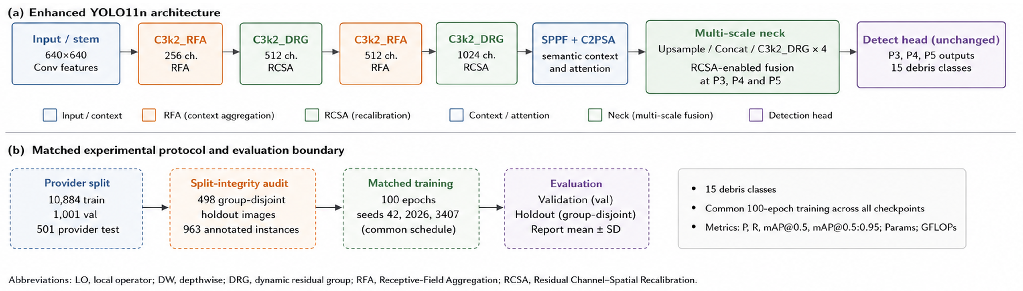
Figure 1 presents an implementation-faithful overview of the revised study, separating the enhanced feature pathway from the matched experimental protocol and evaluation boundary. RFA is used in selected backbone blocks to aggregate context over multiple receptive fields, whereas RCSA is applied through dynamic residual groups in the enhanced feature pathway. The YOLO detection head remains unchanged.

The placement of the two modules reflects the failure modes observed in the baseline. RFA operates where local features are formed, whereas RCSA acts on representations that have already been enriched and fused. Their functions are therefore complementary rather than interchangeable.

3.2. Dataset and Application Context

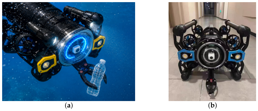
The detector is investigated as a lightweight candidate for compact ROVs used in seabed surveys, harbor inspection, cable and mooring inspection, and related marine-monitoring tasks. The authors participated in related experiments with the commercially available open-source ROV shown in Figure 2; the vehicle itself was not designed or manufactured by the authors. The photographs document the application context only. The detector reported in this study was evaluated on the workstation and image datasets described below, and no onboard latency, power, or energy result is claimed.

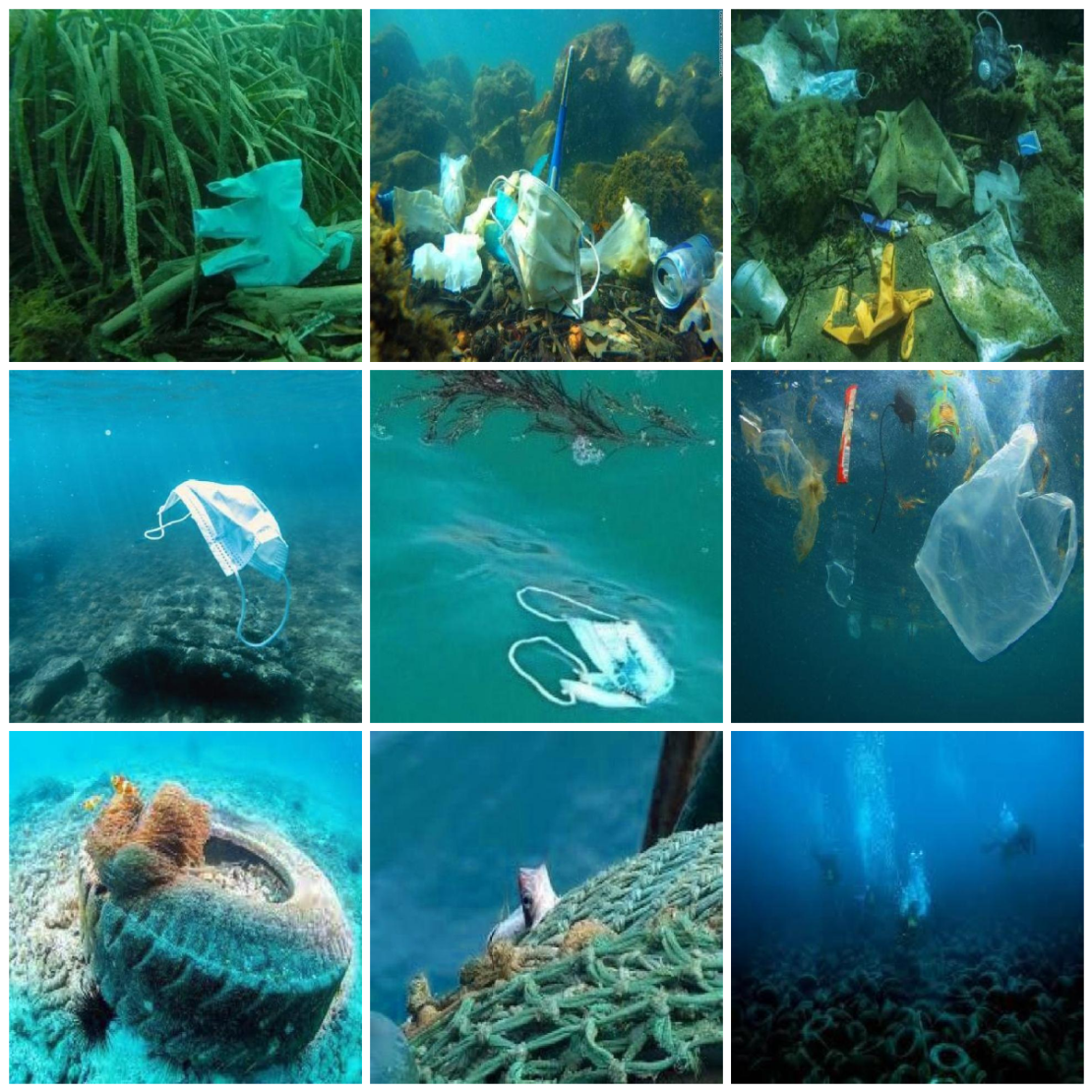
The original provider split contains 10,884 training images, 1001 validation images, and 501 test images [44]. Exact SHA-256 duplicate checks and filename-derived provenance identifiers were used to audit the candidate holdout. Images whose audited provenance groups also appeared in training or validation were excluded from the holdout, leaving 498 test images and 963 annotated objects. (See Figure 3). Model selection used the original provider training and validation partitions; the audited holdout was used only for final evaluation. This identifier-based audit reduces obvious split overlap but does not prove physical-site independence.

The original validation subset contains 1001 unique images and 1892 annotated objects across 15 classes (See

Table 2. Class distribution in the original provider training and validation partitions.

Class	Train Images	Val Images	Total Images	Train Instances	Val Instances	Total Instances
mask	1367	77	1444	4310	90	4400
can	265	18	283	370	20	390
cellphone	702	61	763	804	71	875
electronics	291	27	318	411	40	451
gbottle	480	36	516	1017	82	1099
glove	1265	37	1302	3501	55	3556
metal	90	10	100	168	22	190
misc	510	49	559	519	52	571
net	1503	146	1649	1596	148	1744
pbag	2908	290	3198	3397	330	3727
pbottle	1440	122	1562	2790	284	3074
plastic	411	51	462	530	59	589
rod	51	7	58	78	9	87
sunglasses	42	3	45	42	3	45
tire	1464	143	1607	6816	627	7443

Note: Image counts in this table are reported on a per-class basis. Because one image may contain multiple categories, these counts overlap and must not be summed to obtain the number of unique images.

). Its class distribution is markedly imbalanced. After the split-integrity audit, a subset of the provider test partition containing 498 images and 963 objects was retained, was group-disjoint according to filename-derived provenance identifiers, and was not used for training or checkpoint selection. Validation tables refer to the 1001-image model-selection split, whereas final-model holdout results refer to the audited test subset. Because both subsets originate from the same public dataset, cross-dataset generalization remains untested.

3.3. Baseline and Improved Network Structures

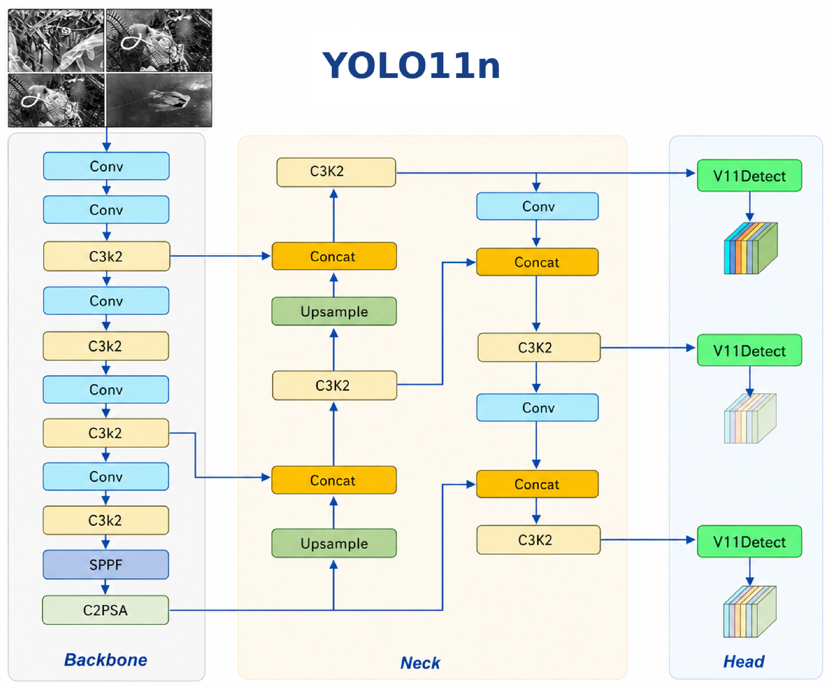
The baseline follows the standard backbone–neck–head organization shown in Figure 4. Hierarchical features are extracted in the backbone, combined across scales in the neck, and passed to three detection branches [32].

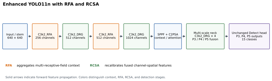
The improved network is shown in Figure 5. In the implementation, C3k2_RFA denotes a C3k2 block incorporating receptive-field aggregation (See

Table 3. Implementation roles of the proposed network modifications.

Component	Network Location	Operation and Output Handling
C3k2_RFA	Backbone feature-extraction stage	Multi-branch local operators aggregate responses with different effective receptive fields before 1 × 1 fusion. The host-stage spatial resolution and channel width are retained.
DRG–RCSAB (RCSA)	Selected backbone and neck blocks	Channel and spatial attention are embedded in a residual group to recalibrate fused features while retaining shortcut information. Identity or projection shortcut P(·) aligns dimensions, and the detection head is unchanged.

). Blocks labeled C3k2_DynamicResidualGroup are used at the enhanced backbone and neck positions shown in Figure 5. Each dynamic residual group (DRG) contains a Residual Channel-Spatial Attention Block (RCSAB) detailed in Section 3.5; this DRG–RCSAB enhancement is referred to as RCSA throughout the manuscript. The detection head remains unchanged.

3.4. RFA Module

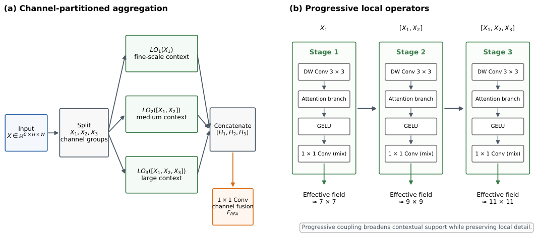
Figure 6 illustrates the RFA mechanism through channel-partitioned aggregation and progressively coupled local operators. The upper panel shows how grouped features are processed and concatenated before 1 × 1 fusion, while the lower panel summarizes the increasing effective receptive fields used to broaden contextual support.

Let $X_i$ denote the ith channel partition of the input feature X, and let ${\mathrm{LO}}_i(·)$ denote the corresponding local operator. The aggregated feature is

$$F_{\mathrm{RFA}}={\mathrm{Conv}}_{1\times 1}\left(\mathrm{Concat}\left[{\mathrm{LO}}_1\left(X_1\right),{\mathrm{LO}}_2\left(X_2\right),\dots ,{\mathrm{LO}}_N\left(X_N\right)\right]\right).$$

(1)

Here, Concat denotes channel concatenation, and ${\mathrm{Conv}}_{1\times 1}$ fuses the branch outputs. This operation broadens contextual representation without replacing the complete lightweight backbone.

3.5. RCSA Module

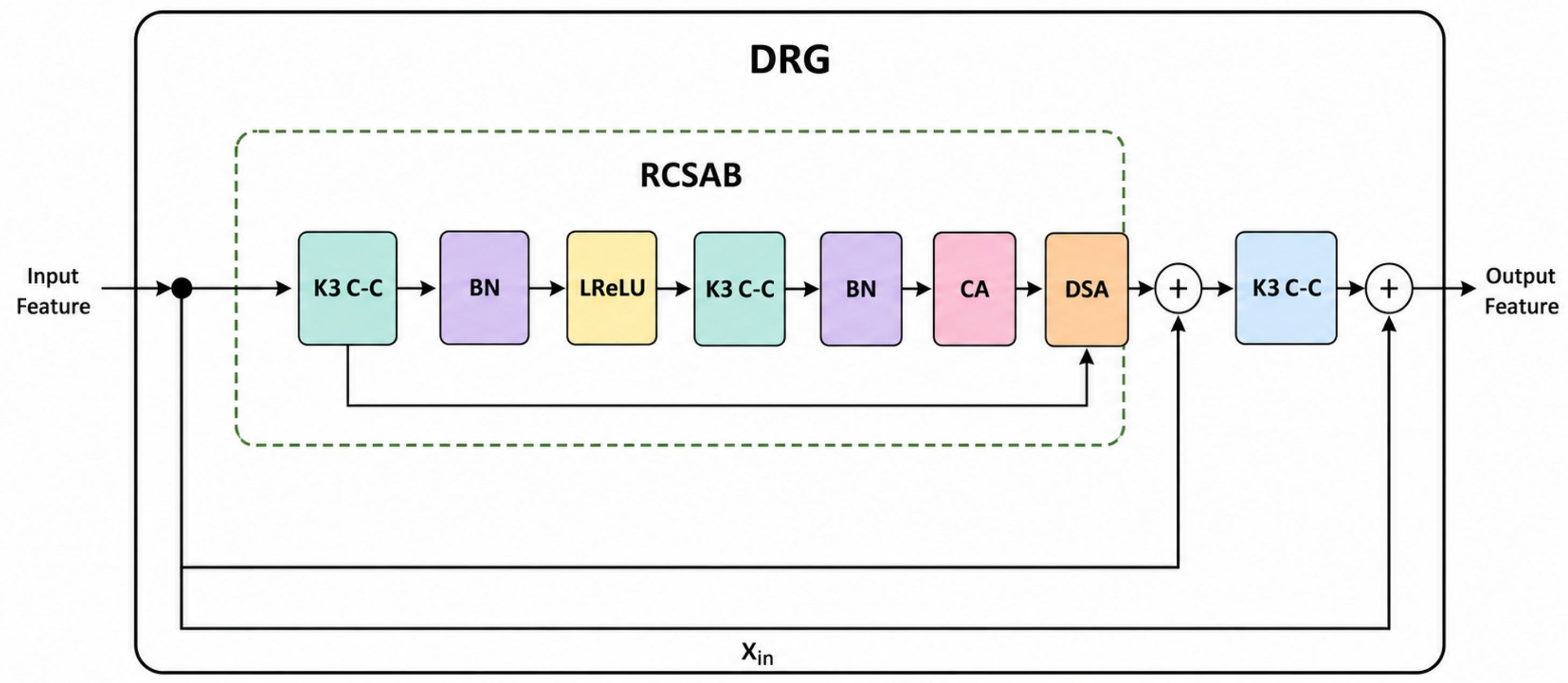
Figure 7 details the implemented RCSA connections. Each RCSAB applies two 3 × 3 convolutions; the first is followed by batch normalization and LeakyReLU, and the second by batch normalization. Channel attention combines global-average and global-maximum descriptors through a shared two-layer 1 × 1 transformation. Dynamic spatial attention generates one sample-specific 3 × 3 kernel from globally pooled features, applies grouped convolution to the channel-mean projection, and multiplies the sigmoid spatial mask with the channel-recalibrated tensor. Each RCSAB has a local residual connection. Four RCSABs and a terminal 3 × 3 convolution form a dynamic residual group with an outer shortcut. Within the C2 Position-Sensitive Attention (C2PSA) host block, one channel branch bypasses the group, the other traverses the dynamic residual and feed-forward paths, and the branches are concatenated and fused by a final 1 × 1 convolution.

Let $T(·)$ denote the two convolution–normalization transformations before the attention operations, $M_c$ and $M_s$ denote the channel- and spatial-attention maps, respectively, and $G(·)$ denote the output convolution. The RCSAB transformation is

$$\begin{array}{cc}\hfill F& =T\left(X\right),\hfill \end{array}$$

(2)

$$\begin{array}{cc}\hfill F_c& =M_c\left(F\right)\odot F,\hfill \end{array}$$

(3)

$$\begin{array}{cc}\hfill F_{cs}& =M_s\left(F_c\right)\odot F_c,\hfill \end{array}$$

(4)

$$\begin{array}{cc}\hfill F_{\mathrm{out}}& =P\left(X\right)+G\left(F_{cs}\right),\hfill \end{array}$$

(5)

where ⊙ denotes element-wise multiplication. $P(·)$ is an identity mapping when dimensions match and a projection mapping otherwise. The attention maps are implemented as

$$\begin{array}{cc}\hfill M_c\left(F\right)& =\sigma \left(W_2\delta \left(W_1\mathrm{GAP}\left(F\right)\right)+W_2\delta \left(W_1\mathrm{GMP}\left(F\right)\right)\right),\hfill \end{array}$$

(6)

$$\begin{array}{cc}\hfill K\left(F_c\right)& =\mathrm{reshape}\left(W_{k2}\delta \left(W_{k1}\mathrm{GAP}\left(F_c\right)\right)\right)\in {\mathbb{R}}^{1\times 3\times 3},\hfill \end{array}$$

(7)

$$\begin{array}{cc}\hfill M_s\left(F_c\right)& =\sigma \left(K\left(F_c\right)\ast {\mathrm{mean}}_c\left(F_c\right)\right),\hfill \end{array}$$

(8)

where GAP and GMP denote global average and maximum pooling, $\delta$ is ReLU, $K\left(F_c\right)$ is the sample-conditioned $3\times 3$ spatial kernel, ${\mathrm{mean}}_c$ is the channel-mean projection, ∗ denotes sample-wise grouped convolution, and $\sigma$ is the sigmoid function.

3.6. Evaluation Metrics

Precision, Recall, mean average precision at IoU 0.5 (mAP@0.5), and mAP@0.5:0.95 are used as the main evaluation metrics. Precision reflects the proportion of correct predictions among all predicted boxes, while Recall reflects the proportion of real objects that are correctly detected. The F1 score evaluates the balance between Precision and Recall:

$$\begin{gathered} \mathrm{Precision}=\left(\mathrm{TP}\right)/(\mathrm{TP}+\mathrm{FP}),\mathrm{Recall}=\left(\mathrm{TP}\right)/(\mathrm{TP}+\mathrm{FN}), \\ \mathrm{F}\_1=\left(2\mathrm{PR}\right)/(\mathrm{P}+\mathrm{R}), \end{gathered}$$

where TP, FP, and FN denote true positives, false positives, and false negatives, respectively. The mean average precision is the mean of the class-wise average-precision values. mAP@0.5 uses an intersection-over-union (IoU) threshold of 0.5, whereas mAP@0.5:0.95 averages across IoU thresholds from 0.5 to 0.95 in increments of 0.05.

4. Experimental Results and Analysis

4.1. Experimental Environment and Training Configuration

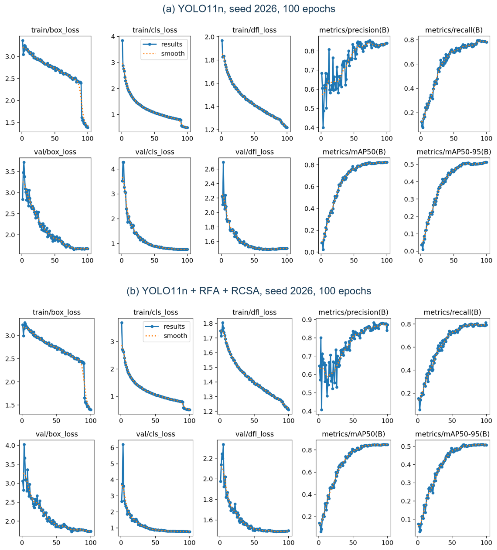
All architecture-screening runs used a common 100-epoch schedule with the same source split, input size, batch size, augmentation settings, and pretrained initialization. Initial module screening used seed 42. For the principal duration-matched comparison, YOLO11n, YOLO11n + RFA, YOLO11n + RCSA, and YOLO11n + RFA + RCSA were each evaluated at seeds 42, 2026, and 3407 (See

Table 4. Experimental environment and training configuration.

Item	Configuration
Hardware	Intel Xeon Gold 5220 CPU (Intel Corporation, Santa Clara, CA, USA); 32 GB memory; NVIDIA GeForce RTX 5070 12 GB GPU (NVIDIA Corporation, Santa Clara, CA, USA)
Software	Windows 11 (Microsoft Corporation, Redmond, WA, USA); Python 3.11.14 (https://www.python.org, accessed on 29 July 2026); PyTorch 2.9.0 (https://pytorch.org, accessed on 29 July 2026); CUDA 12.8 and NVIDIA Driver 595.79 (NVIDIA Corporation)
Framework	Ultralytics YOLO11 training pipeline implemented in PyTorch [32]
Input and batch	Input size 640 × 640; batch size 30
Preprocessing and augmentation	Resize/normalize; hsv_h = 0.015, hsv_s = 0.7, hsv_v = 0.4; translate = 0.1; scale = 0.5; horizontal flip = 0.5; Mosaic = 1.0; degrees = 0; vertical flip = 0; MixUp = 0
Common architecture schedule	100 epochs for YOLO11n, YOLO11n + RFA, YOLO11n + RCSA, and YOLO11n + RFA + RCSA
Repeated-seed protocol	Seeds 42, 2026, and 3407 for YOLO11n, YOLO11n + RFA, YOLO11n + RCSA, and YOLO11n + RFA + RCSA; deterministic mode enabled
Optimization	Ultralytics 8.3.163 optimizer = auto selected Nesterov SGD; initial lr = 0.01; momentum = 0.9; nominal weight decay = 0.0005 (effective 0.00046875 for batch 30, accumulation 2, nbs = 64); warm-up = 3 epochs; patience = 100
Initialization	Pretrained yolo11n.pt weights; AMP enabled
Learning-rate schedule	Linear decay (cos_lr = false); final ten epochs without Mosaic (close_mosaic = 10)
Holdout evaluation	Group-disjoint test split; 498 images, 963 instances; not used for checkpoint selection

). No result from the earlier unmatched 150-epoch fusion run is used in the principal tables or figures.

4.2. Convergence and Training Process

Figure 8 documents the matched experimental design used for the principal comparison. Rather than retaining an unmatched historical convergence plot, it records the shared 100-epoch schedule, seeds, and holdout boundary that make the comparison in

Table 5. Duration-matched 100-epoch validation comparison. All four models are reported as mean ± standard deviation over seeds 42, 2026, and 3407.

Model	Epochs	Runs/Seeds	Precision	Recall	mAP@0.5	mAP@0.5:0.95
YOLO11n	100	3: 42, 2026, 3407	0.851 ± 0.021	0.769 ± 0.012	0.819 ± 0.008	0.506 ± 0.005
YOLO11n + RFA	100	3: 42, 2026, 3407	0.832 ± 0.006	0.788 ± 0.014	0.831 ± 0.002	0.509 ± 0.005
YOLO11n + RCSA	100	3: 42, 2026, 3407	0.830 ± 0.015	0.781 ± 0.012	0.810 ± 0.005	0.509 ± 0.004
YOLO11n + RFA + RCSA	100	3: 42, 2026, 3407	0.861 ± 0.016	0.801 ± 0.012	0.848 ± 0.001	0.511 ± 0.002

interpretable.

Detailed run-level outputs, split-audit records, and supporting experimental files are provided in Supplementary Materials S1–S5.

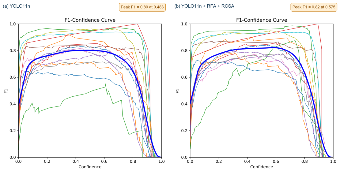
Figure 9 compares the F1–confidence curves of YOLO11n and YOLO11n + RFA + RCSA. Each colored curve represents the F1–confidence relationship for an individual debris class, while the thick blue curve represents the aggregated performance across all 15 classes. The annotated point indicates the confidence threshold at which the highest overall F1 score is obtained.

4.3. Module Screening and RFA-Centered Combinations

Each candidate module and RFA-centered pairing was trained for 100 epochs. The single-module and initial pairing rows in

Table 6. Unified single-module and RFA-centered screening under the common 100-epoch schedule.

Group	Model	Epochs	Runs	Precision	Recall	mAP@0.5	mAP@0.5:0.95
Single module (seed 42)	YOLO11n	100	1	0.836	0.770	0.810	0.502
	YOLO11n + RFA	100	1	0.833	0.787	0.832	0.515
	YOLO11n + CSA_ConvBlock	100	1	0.858	0.771	0.814	0.510
	YOLO11n + Di_SpAM	100	1	0.801	0.723	0.773	0.478
	YOLO11n + RCSA	100	1	0.830	0.781	0.810	0.509
	YOLO11n + CoordAtt	100	1	0.798	0.765	0.799	0.493
	YOLO11n + iRMB	100	1	0.837	0.725	0.783	0.482
RFA pairing (seed 42)	RFA + CoordAtt	100	1	0.853	0.740	0.805	0.494
	RFA + DySample + ECA	100	1	0.864	0.765	0.796	0.485
	RFA + Di_SpAM	100	1	0.756	0.696	0.747	0.473
	RFA + CSA_ConvBlock	100	1	0.826	0.748	0.815	0.500
Selected model	RFA + RCSA	100	3	0.861 ± 0.016	0.801 ± 0.012	0.848 ± 0.001	0.511 ± 0.002

are seed-42 screening results, whereas the selected RFA + RCSA row reports the three-seed mean. The formal duration-matched comparison is reported separately in Table 5.

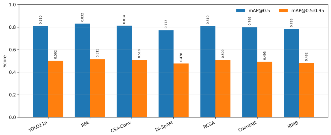
RFA yields the strongest mAP values among the single-module variants. Relative to YOLO11n, mAP@0.5 increases by 2.2 percentage points and mAP@0.5:0.95 by 1.3 percentage points (See Figure 10). CSA_ConvBlock achieves the highest Precision, although its Recall and mAP gains are smaller. When used alone, RCSA changes the aggregate metrics only slightly, suggesting that its contribution may depend on a sufficiently informative contextual representation.

4.4. Architecture Screening and Final-Model Training

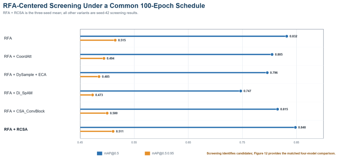
RFA was paired with several enhancement blocks to test whether its contextual gain was retained after feature fusion. Figure 11 summarizes the RFA-centered screening rows consolidated in Table 6.

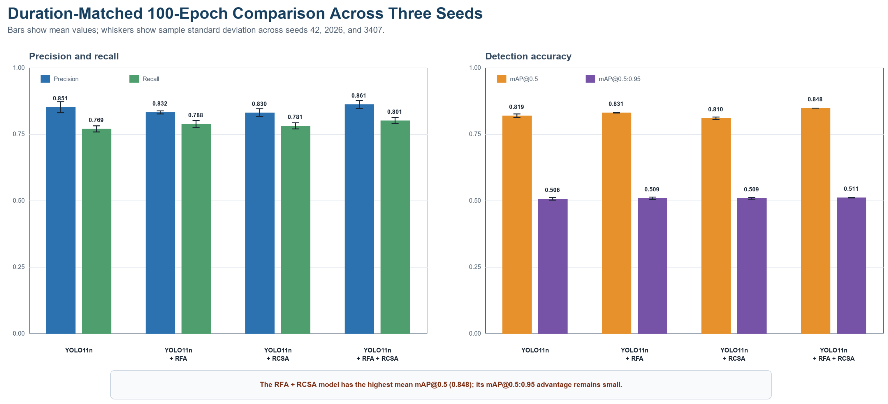
Figure 12 summarizes the validation outcomes used for the final comparison.

None of the alternative single-seed RFA combinations in Table 6 exceeds RFA alone in mAP@0.5:0.95. RCSA was retained because it performs residual channel-spatial recalibration rather than adding another receptive-field or resampling operation. The selected fusion was then evaluated for 100 epochs at seeds 42, 2026, and 3407, matching the baseline and RFA duration.

4.5. Overall Performance and Complexity Analysis

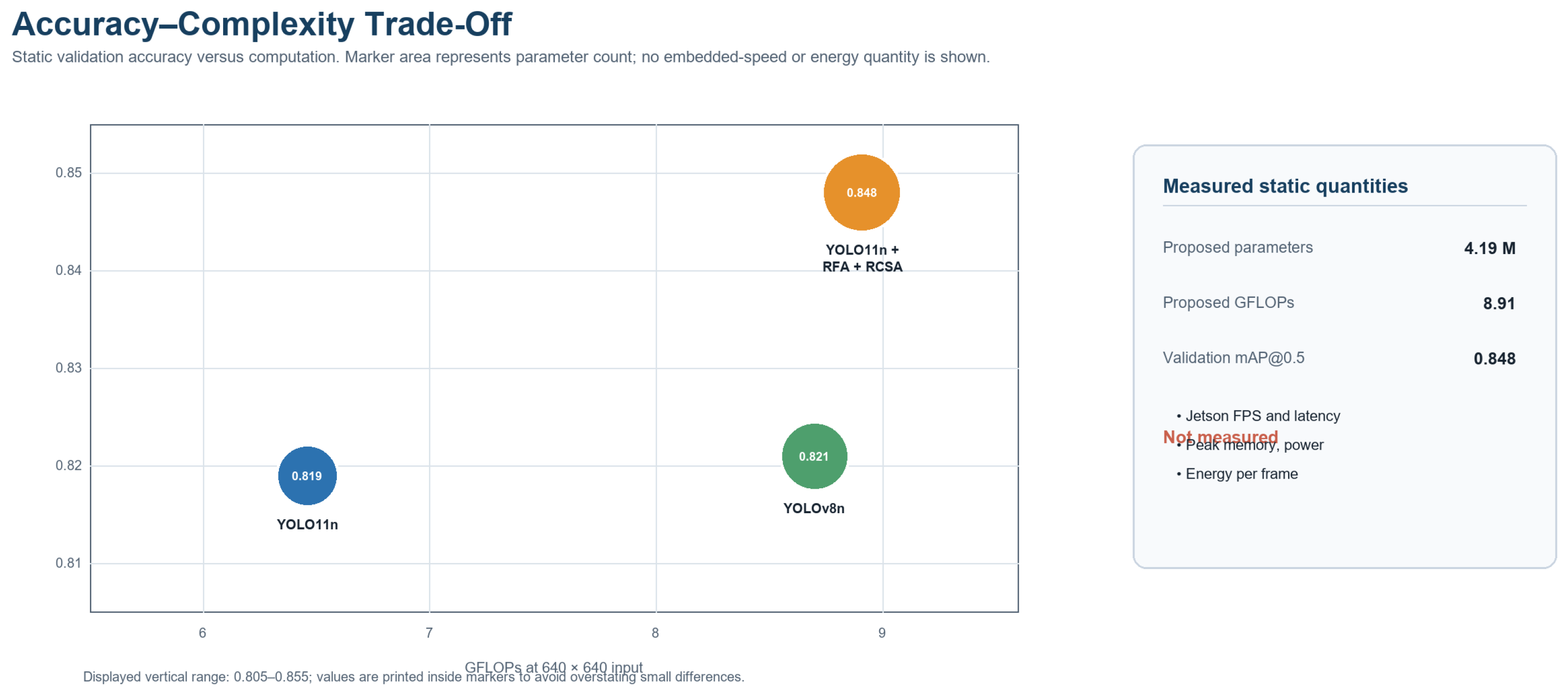
The implemented RFA + RCSA network contains 4.19 M parameters and requires 8.91 giga floating-point operations (GFLOPs) at 640 × 640 input resolution (See

Table 7. Computational complexity and embedded-deployment measurement status of the evaluated models.

Model	Params/M	GFLOPs	Weights/MB	Embedded Measurement Status	mAP@0.5	mAP@0.5:0.95
YOLO11n	2.59	6.46	5.23	Not measured	0.819 ± 0.008	0.506 ± 0.005
YOLO11n + RFA	2.60	6.63	5.25	Not measured	0.831 ± 0.002	0.509 ± 0.005
YOLO11n + RFA + RCSA	4.19	8.91	8.43	Not measured	0.848 ± 0.001	0.511 ± 0.002

). The three matched seeds permit an exploratory paired comparison only. Relative to RFA, the fusion increases validation mAP@0.5 by 0.0178 (paired 95% CI 0.0103–0.0253; paired t-test p = 0.009 under the normal-difference assumption). The mAP@0.5:0.95 difference is 0.0021 (95% CI −0.0150–0.0191; p = 0.654), so a stricter-IoU improvement is not established. Because n = 3 is small, these statistics quantify observed run-to-run variation rather than providing definitive evidence of general superiority (See

Table 8. Same-dataset validation comparison with YOLOv8n. Runs are identified; embedded FPS, latency, peak memory, power, and energy per frame were not measured.

Model	Runs	Params/M	GFLOPs	Embedded Measurement Status	Precision	Recall	mAP@0.5	mAP@0.5:0.95
YOLOv8n	1	3.20	8.70	Not measured	0.842	0.779	0.821	0.508
YOLO11n	3	2.59	6.46	Not measured	0.851 ± 0.021	0.769 ± 0.012	0.819 ± 0.008	0.506 ± 0.005
YOLO11n + RFA + RCSA	3	4.19	8.91	Not measured	0.861 ± 0.016	0.801 ± 0.012	0.848 ± 0.001	0.511 ± 0.002

). The results therefore support a cautious moderate-IoU gain while requiring a restrained interpretation of localization accuracy.

YOLOv8n is included only as a representative lightweight detector evaluated on the same source dataset. The present revision does not report an embedded FPS value because no Jetson-class experiment was performed. Desktop-GPU timing is not used to claim real-time ROV deployment. A valid deployment study must report end-to-end latency, FPS, peak memory, power, and energy per frame on the target hardware under a declared precision mode and batch size (See Figure 13).

4.6. Class-Wise AP and Long-Tail Analysis

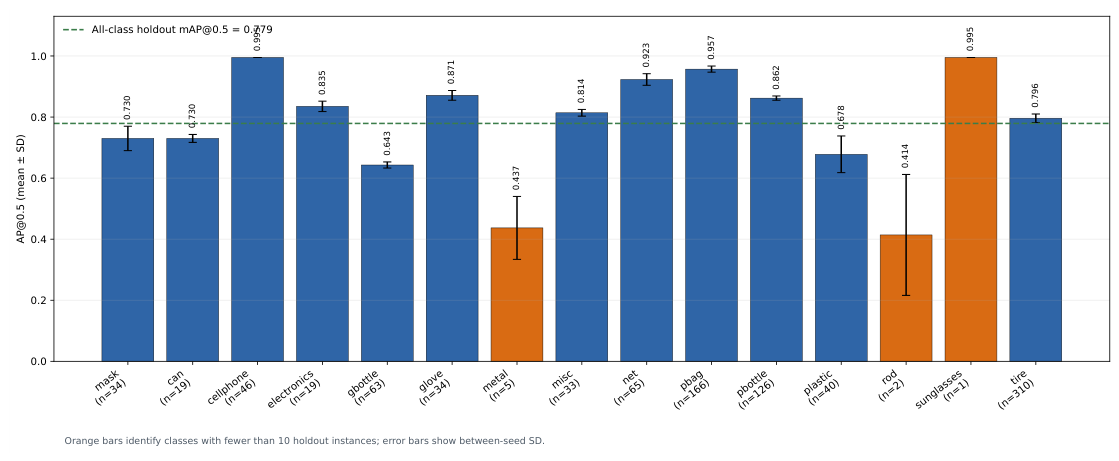
Figure 14 and

Table 9. Class-wise audited-holdout AP@0.5 (the bold row is the all-class aggregate), reported as mean ± standard deviation and a between-seed 95% t interval across seeds 42, 2026, and 3407.

Class	Test Inst.	AP@0.5 Mean ± SD [95% CI]	Class	Test Inst.	AP@0.5 Mean ± SD [95% CI]
mask	34	0.730 ± 0.040 [0.630, 0.831]	net	65	0.923 ± 0.019 [0.876, 0.969]
can	19	0.730 ± 0.013 [0.697, 0.762]	pbag	166	0.957 ± 0.010 [0.931, 0.982]
cellphone	46	0.995 ± 0.000 [0.995, 0.995]	pbottle	126	0.862 ± 0.007 [0.844, 0.881]
electronics	19	0.835 ± 0.017 [0.793, 0.877]	plastic	40	0.678 ± 0.060 [0.529, 0.827]
gbottle	63	0.643 ± 0.010 [0.618, 0.667]	rod	2	0.414 ± 0.198 [0.000, 0.907]
glove	34	0.871 ± 0.016 [0.830, 0.911]	sunglasses	1	0.995 ± 0.000 [0.995, 0.995]
metal	5	0.437 ± 0.103 [0.182, 0.692]	tire	310	0.796 ± 0.014 [0.760, 0.831]
misc	33	0.814 ± 0.011 [0.788, 0.841]	all classes	963	0.779 ± 0.018 [0.734, 0.823]

relate class-wise AP@0.5 to the number of instances in the filename-provenance group-disjoint holdout and report between-seed variability across the three RFA + RCSA checkpoints.

The audited holdout results confirm pronounced long-tail uncertainty. Rod has only two instances and AP@0.5 = 0.414 ± 0.198; the single sunglasses instance yields AP@0.5 = 0.995 for all three checkpoints but is not evidence of broad generalization. The intervals quantify between-seed variation, not image-sampling uncertainty. Focal-loss and class-balanced-loss strategies are established alternatives for such imbalance [45,46]. Here, an exploratory $4\times$ rare-class oversampling experiment was conducted using the original 10,884-image training partition; sampling frequency was changed, and no unique or synthetic images were added. Its aggregate holdout result is reported in

Table 10. Additional measured evaluations. Values are mean ± standard deviation over the three completed RFA + RCSA checkpoints; no values in this table are simulated.

Evaluation	Data/Protocol	mAP@0.5	mAP@0.5:0.95	Interpretation
Reference holdout	Audited group-disjoint holdout; 498 images/963 instances	0.779 ± 0.018	0.467 ± 0.007	Unmodified reference evaluation.
Brightness 0.70	Same 498-image/963-instance holdout; test-time transform	0.776 ± 0.019	0.469 ± 0.002	Within the observed seed variation.
Brightness 1.30	Same 498-image/963-instance holdout; test-time transform	0.773 ± 0.022	0.466 ± 0.006	Small average change.
Contrast 0.70	Same 498-image/963-instance holdout; test-time transform	0.644 ± 0.025	0.397 ± 0.014	Substantial degradation under reduced contrast.
Contrast 1.30	Same 498-image/963-instance holdout; test-time transform	0.728 ± 0.019	0.427 ± 0.004	Moderate degradation.
$4\times$ rare-class oversampling	Original training partition (10,884 unique images); sampling frequency only; no new or synthetic images; metal, rod, and sunglasses sampled $4\times$	0.772 ± 0.006	0.464 ± 0.007	No overall holdout improvement over the reference protocol.
External material-domain test	TrashCan Material metal/plastic subset; 1204 images, 599 mapped target instances	0.031 ± 0.023	0.017 ± 0.012	Severe taxonomy and domain shift; not evidence of cross-domain robustness.

and does not demonstrate an overall improvement.

4.7. Robustness, Long-Tail, and External Generalization

All supplementary evaluations used fixed, previously unseen data and the three completed RFA + RCSA checkpoints (seeds 42, 2026, and 3407). Photometric transformations were applied only at test time to the same audited group-disjoint holdout (498 images; 963 annotated instances), so the observed changes quantify sensitivity to appearance perturbations rather than a retraining effect.

The brightness factors produced changes smaller than or comparable with between-seed variation, whereas low contrast caused the largest performance reduction. The exploratory rare-class oversampling comparison did not improve aggregate holdout mAP and is reported as a negative control rather than as a performance claim. The external material-domain test is deliberately retained despite its low score because it demonstrates that same-source holdout performance does not establish cross-dataset generalization.

5. Discussion

5.1. Interpretation of the Detection Results

The duration-matched experiments indicate that contextual representation is a major limitation of the baseline. RFA improves validation mAP@0.5 under the common 100-epoch schedule, while several other attention or resampling combinations do not preserve that gain. This contrast shows that additional modules are not automatically beneficial and motivates explicit ablation rather than complexity-driven design.

RCSA serves a different role from RFA: it adjusts channel and spatial responses after contextual enrichment. With matched seeds and 100 epochs, RFA + RCSA shows a higher mean validation mAP@0.5 than RFA, whereas the difference in mAP@0.5:0.95 remains small. The evidence therefore supports an observed moderate-IoU detection gain while remaining inconclusive for stricter localization quality.

Brightness and contrast affect detection through different failure modes. The completed test-time robustness study shows that brightness factors of 0.70 and 1.30 caused only small mean changes on the audited holdout, while contrast 0.70 reduced mAP@0.5 from 0.779 ± 0.018 to 0.644 ± 0.025 and mAP@0.5:0.95 from 0.467 ± 0.007 to 0.397 ± 0.014. Contrast 1.30 produced an intermediate reduction (mAP@0.5 = 0.728 ± 0.019). These results indicate that weak target–background separation is the more consequential photometric failure mode in this protocol.

5.2. Sustainability Relevance and Boundary of Claims

The proposed detector is positioned as a lightweight perception candidate for resource-constrained ROV-assisted debris mapping, inventory, and removal planning. If integrated with navigation and georeferencing, its detections could support recurring monitoring of seabed habitats, ports, mooring zones, subsea cables, and offshore renewable-energy facilities. This prospective use is consistent with SDG 14, but the present experiments validate the detector rather than a complete field-deployed monitoring system.

The sustainability claim is deliberately bounded. This study measures recognition accuracy and computational complexity; it does not measure debris-removal rates, biodiversity recovery, life-cycle impacts, energy use, or carbon emissions. No Jetson-class FPS, end-to-end latency, peak memory, power, or energy-per-frame result is reported. Post-training compression methods such as distribution-aware residual entropy quantization [43] may be investigated for future resource-limited deployment, but are not used here as detection baselines or evidence of embedded performance.

5.3. Limitations and Future Validation

Four limitations remain. First, the group-disjoint holdout is derived from the same public source dataset, and the additional TrashCan Material test shows severe cross-dataset degradation; broader underwater cross-dataset evaluation is still required. Second, three seeds provide only a small-sample uncertainty estimate. Third, rare classes remain statistically underpowered, and the present $4\times$ oversampling control did not improve aggregate holdout performance. Fourth, real ROV motion, turbidity, and Jetson-class latency, FPS, peak memory, power, and energy per frame have not been measured. Future work will prioritize rare-class data acquisition and loss-function studies, embedded profiling, and field validation under realistic underwater dynamics.

6. Conclusions

This study presents a compact YOLO11n-based detector for underwater marine-debris recognition. Existing RFA and dynamic residual-group concepts are adapted and integrated at complementary locations: RFA strengthens contextual extraction, while RCSA recalibrates enriched channel and spatial responses. All principal comparisons use 100 epochs, removing the duration mismatch identified in the earlier manuscript.

Across three matched seeds, RFA + RCSA achieved validation mAP@0.5 of 0.848 ± 0.001 and mAP@0.5:0.95 of 0.511 ± 0.002. On the audited holdout, the corresponding means were 0.779 ± 0.018 and 0.467 ± 0.007. These three-run estimates should be read as reproducibility evidence within one public source, not as site-level or cross-dataset proof. The photometric test identifies reduced contrast as a material failure condition, while the rare-class oversampling control and external material-domain evaluation do not support a claim of general robustness. Operationally, the detector addresses conversion of underwater inspection imagery into repeatable debris locations and class inventories that can support survey prioritization and human-supervised removal planning; it does not by itself quantify ecological recovery. With 4.19 M parameters and 8.91 GFLOPs, the design is a lightweight candidate for resource-constrained ROV perception, not a demonstrated embedded real-time system.

References

1. United Nations Environment Programme. From Pollution to Solution: A Global Assessment of Marine Litter and Plastic Pollution; UNEP: Nairobi, Kenya, 2021. [Google Scholar]
2. Jambeck, J.R.; Geyer, R.; Wilcox, C.; Siegler, T.R.; Perryman, M.; Andrady, A.; Narayan, R.; Law, K.L. Plastic Waste Inputs from Land into the Ocean. Science 2015, 347, 768–771. [Google Scholar] [CrossRef] [Scilit] [PubMed]
3. Geyer, R.; Jambeck, J.R.; Law, K.L. Production, Use, and Fate of All Plastics Ever Made. Sci. Adv. 2017, 3, e1700782. [Google Scholar] [CrossRef] [Scilit] [PubMed]
4. Eriksen, M.; Lebreton, L.C.M.; Carson, H.S.; Thiel, M.; Moore, C.J.; Borerro, J.C.; Galgani, F.; Ryan, P.G.; Reisser, J. Plastic Pollution in the World’s Oceans: More than 5 Trillion Plastic Pieces Weighing over 250,000 Tons Afloat at Sea. PLoS ONE 2014, 9, e111913. [Google Scholar] [CrossRef] [Scilit] [PubMed]
5. Gregory, M.R. Environmental Implications of Plastic Debris in Marine Settings—Entanglement, Ingestion, Smothering, Hangers-On, Hitch-Hiking and Alien Invasions. Philos. Trans. R. Soc. B 2009, 364, 2013–2025. [Google Scholar] [CrossRef] [Scilit] [PubMed]
6. Cózar, A.; Echevarría, F.; González-Gordillo, J.I.; Irigoien, X.; Úbeda, B.; Hernández-León, S.; Palma, A.T.; Navarro, S.; García-de-Lomas, J.; Ruiz, A.; et al. Plastic Debris in the Open Ocean. Proc. Natl. Acad. Sci. USA 2014, 111, 10239–10244. [Google Scholar] [CrossRef] [Scilit] [PubMed]
7. Lebreton, L.; Slat, B.; Ferrari, F.; Sainte-Rose, B.; Aitken, J.; Marthouse, R.; Hajbane, S.; Cunsolo, S.; Schwarz, A.; Levivier, A.; et al. Evidence that the Great Pacific Garbage Patch Is Rapidly Accumulating Plastic. Sci. Rep. 2018, 8, 4666. [Google Scholar] [CrossRef] [Scilit] [PubMed]
8. United Nations. Transforming Our World: The 2030 Agenda for Sustainable Development; A/RES/70/1; United Nations: New York, NY, USA, 2015. [Google Scholar]
9. Jaffe, J.S. Computer Modeling and the Design of Optimal Underwater Imaging Systems. IEEE J. Ocean. Eng. 1990, 15, 101–111. [Google Scholar] [CrossRef] [Scilit]
10. McGlamery, B.L. A Computer Model for Underwater Camera Systems. In Proceedings of Ocean Optics VI; SPIE: Bellingham, WA, USA, 1980; Volume 208, pp. 221–231. [Google Scholar]
11. Akkaynak, D.; Treibitz, T. A Revised Underwater Image Formation Model. In Proceedings of the IEEE/CVF Conference on Computer Vision and Pattern Recognition, Salt Lake City, UT, USA, 18–23 June 2018; pp. 6723–6732. [Google Scholar]
12. Ancuti, C.O.; Ancuti, C.; Haber, T.; Bekaert, P. Enhancing Underwater Images and Videos by Fusion. In Proceedings of the IEEE Conference on Computer Vision and Pattern Recognition, Providence, RI, USA, 16–21 June 2012; pp. 81–88. [Google Scholar]
13. Li, C.; Guo, C.; Ren, W.; Cong, R.; Hou, J.; Kwong, S.; Tao, D. An Underwater Image Enhancement Benchmark Dataset and Beyond. IEEE Trans. Image Process. 2020, 29, 4376–4389. [Google Scholar] [CrossRef] [Scilit] [PubMed]
14. Islam, M.J.; Xia, Y.; Sattar, J. Fast Underwater Image Enhancement for Improved Visual Perception. IEEE Robot. Autom. Lett. 2020, 5, 3227–3234. [Google Scholar] [CrossRef] [Scilit]
15. Redmon, J.; Divvala, S.; Girshick, R.; Farhadi, A. You Only Look Once: Unified, Real-Time Object Detection. In Proceedings of the IEEE Conference on Computer Vision and Pattern Recognition, Las Vegas, NV, USA, 27–30 June 2016; pp. 779–788. [Google Scholar]
16. Bochkovskiy, A.; Wang, C.-Y.; Liao, H.-Y.M. YOLOv4: Optimal Speed and Accuracy of Object Detection. arXiv 2020, arXiv:2004.10934. [Google Scholar]
17. Liu, W.; Anguelov, D.; Erhan, D.; Szegedy, C.; Reed, S.; Fu, C.-Y.; Berg, A.C. SSD: Single Shot MultiBox Detector. In Proceedings of the European Conference on Computer Vision, Amsterdam, The Netherlands, 11–14 October 2016; pp. 21–37. [Google Scholar]
18. Lin, T.-Y.; Dollár, P.; Girshick, R.; He, K.; Hariharan, B.; Belongie, S. Feature Pyramid Networks for Object Detection. In Proceedings of the IEEE Conference on Computer Vision and Pattern Recognition, Honolulu, HI, USA, 21–26 July 2017; pp. 2117–2125. [Google Scholar]
19. Liu, S.; Qi, L.; Qin, H.; Shi, J.; Jia, J. Path Aggregation Network for Instance Segmentation. In Proceedings of the IEEE/CVF Conference on Computer Vision and Pattern Recognition, Salt Lake City, UT, USA, 18–23 June 2018; pp. 8759–8768. [Google Scholar]
20. Tan, M.; Pang, R.; Le, Q.V. EfficientDet: Scalable and Efficient Object Detection. In Proceedings of the IEEE/CVF Conference on Computer Vision and Pattern Recognition, Seattle, WA, USA, 13–19 June 2020; pp. 10781–10790. [Google Scholar]
21. Ge, Z.; Liu, S.; Wang, F.; Li, Z.; Sun, J. YOLOX: Exceeding YOLO Series in 2021. arXiv 2021, arXiv:2107.08430. [Google Scholar]
22. Wang, C.-Y.; Bochkovskiy, A.; Liao, H.-Y.M. YOLOv7: Trainable Bag-of-Freebies Sets New State-of-the-Art for Real-Time Object Detectors. In Proceedings of the IEEE/CVF Conference on Computer Vision and Pattern Recognition, Vancouver, BC, Canada, 18–22 June 2023; pp. 7464–7475. [Google Scholar]
23. Zhang, X.; Liu, C.; Yang, D.; Song, T.; Ye, Y.-C.; Li, K.; Song, Y.-Z. RFAConv: Receptive-Field Attention Convolution for Improving Convolutional Neural Networks. arXiv 2023, arXiv:2304.03198. [Google Scholar]
24. Xiong, Z.; Zhou, F.; Wu, F.; Yuan, S.; Fu, M.; Peng, Z.; Yang, J.; Dai, Y. DRPCA-Net: Make Robust PCA Great Again for Infrared Small Target Detection. IEEE Trans. Geosci. Remote Sens. 2025, 63, 5005516. [Google Scholar] [CrossRef] [Scilit]
25. Fulton, M.; Hong, J.; Islam, M.J.; Sattar, J. Robotic Detection of Marine Litter Using Deep Visual Detection Models. In Proceedings of the IEEE International Conference on Robotics and Automation, Montreal, QC, Canada, 20–24 May 2019; pp. 5752–5758. [Google Scholar]
26. Hong, J.; Fulton, M.; Sattar, J. TrashCan: A Semantically-Segmented Dataset towards Visual Detection of Marine Debris. arXiv 2020, arXiv:2007.08097. [Google Scholar]
27. Islam, M.J.; Edge, C.; Xiao, Y.; Luo, P.; Mehtaz, M.; Morse, C.; Enan, S.S.; Sattar, J. Semantic Segmentation of Underwater Imagery: Dataset and Benchmark. In Proceedings of the 2020 IEEE/RSJ International Conference on Intelligent Robots and Systems, Las Vegas, NV, USA, 24 October 2020–24 January 2021; pp. 1769–1776. [Google Scholar]
28. Zhao, Y.; Sun, F.; Wu, X. FEB-YOLOv8: A Multi-Scale Lightweight Detection Model for Underwater Object Detection. PLoS ONE 2024, 19, e0311173. [Google Scholar] [CrossRef] [Scilit] [PubMed]
29. Cai, S.; Zhang, X.; Mo, Y. A Lightweight Underwater Detector Enhanced by Attention Mechanism, GSConv and WIoU on YOLOv8. Sci. Rep. 2024, 14, 25797. [Google Scholar] [CrossRef] [Scilit]
30. Huang, C.; Zhang, W.; Zheng, B.; Li, J.; Xie, B.; Nan, R.; Tan, Z.; Tan, B.; Xiong, N.N. YOLO-MES: An Effective Lightweight Underwater Garbage Detection Scheme for Marine Ecosystems. IEEE Access 2025, 13, 60440–60454. [Google Scholar] [CrossRef] [Scilit]
31. Luo, Y.; Eljamal, O. SPyramidLightNet: A Lightweight Shared Pyramid Network for Efficient Underwater Debris Detection. Appl. Sci. 2025, 15, 9404. [Google Scholar] [CrossRef] [Scilit]
32. Ultralytics. Ultralytics YOLO Documentation. Available online: https://docs.ultralytics.com (accessed on 29 July 2026).
33. Sandler, M.; Howard, A.; Zhu, M.; Zhmoginov, A.; Chen, L.-C. MobileNetV2: Inverted Residuals and Linear Bottlenecks. In Proceedings of the IEEE/CVF Conference on Computer Vision and Pattern Recognition, Salt Lake City, UT, USA, 18–23 June 2018; pp. 4510–4520. [Google Scholar]
34. Han, K.; Wang, Y.; Tian, Q.; Guo, J.; Xu, C.; Xu, C. GhostNet: More Features from Cheap Operations. In Proceedings of the IEEE/CVF Conference on Computer Vision and Pattern Recognition, Seattle, WA, USA, 13–19 June 2020; pp. 1580–1589. [Google Scholar]
35. He, K.; Zhang, X.; Ren, S.; Sun, J. Deep Residual Learning for Image Recognition. In Proceedings of the IEEE Conference on Computer Vision and Pattern Recognition, Las Vegas, NV, USA, 27–30 June 2016; pp. 770–778. [Google Scholar]
36. Hu, J.; Shen, L.; Sun, G. Squeeze-and-Excitation Networks. In Proceedings of the IEEE/CVF Conference on Computer Vision and Pattern Recognition, Salt Lake City, UT, USA, 18–23 June 2018; pp. 7132–7141. [Google Scholar]
37. Woo, S.; Park, J.; Lee, J.-Y.; Kweon, I.S. CBAM: Convolutional Block Attention Module. In Proceedings of the European Conference on Computer Vision, Munich, Germany, 8–14 September 2018; pp. 3–19. [Google Scholar]
38. Wang, Q.; Wu, B.; Zhu, P.; Li, P.; Zuo, W.; Hu, Q. ECA-Net: Efficient Channel Attention for Deep Convolutional Neural Networks. In Proceedings of the IEEE/CVF Conference on Computer Vision and Pattern Recognition, Seattle, WA, USA, 13–19 June 2020; pp. 11534–11542. [Google Scholar]
39. Hou, Q.; Zhou, D.; Feng, J. Coordinate Attention for Efficient Mobile Network Design. In Proceedings of the IEEE/CVF Conference on Computer Vision and Pattern Recognition, Nashville, TN, USA, 20–25 June 2021; pp. 13713–13722. [Google Scholar]
40. Li, X.; Wang, W.; Hu, X.; Yang, J. Selective Kernel Networks. In Proceedings of the IEEE/CVF Conference on Computer Vision and Pattern Recognition, Long Beach, CA, USA, 15–20 June 2019; pp. 510–519. [Google Scholar]
41. Wang, X.; Girshick, R.; Gupta, A.; He, K. Non-Local Neural Networks. In Proceedings of the IEEE/CVF Conference on Computer Vision and Pattern Recognition, Salt Lake City, UT, USA, 18–23 June 2018; pp. 7794–7803. [Google Scholar]
42. Liu, W.; Lu, H.; Fu, H.; Cao, Z. Learning to Upsample by Learning to Sample. In Proceedings of the IEEE/CVF International Conference on Computer Vision, Paris, France, 1–6 October 2023; pp. 6027–6037. [Google Scholar]
43. Sakovich, N.; Aksenov, D.; Pleshakova, E.; Gataullin, S. AI Model Compression Methods: A Distribution-Aware Residual Entropy Quantization. Comput. Mater. Contin. 2026, 88, 32. [Google Scholar] [CrossRef] [Scilit]
44. Roboflow Universe. Underwater Waste Dataset. Available online: https://universe.roboflow.com/tasmia0805/underwater_waste (accessed on 29 July 2026).
45. Lin, T.-Y.; Goyal, P.; Girshick, R.; He, K.; Dollár, P. Focal Loss for Dense Object Detection. In Proceedings of the IEEE International Conference on Computer Vision, Venice, Italy, 22–29 October 2017; pp. 2980–2988. [Google Scholar]
46. Cui, Y.; Jia, M.; Lin, T.-Y.; Song, Y.; Belongie, S. Class-Balanced Loss Based on Effective Number of Samples. In Proceedings of the IEEE/CVF Conference on Computer Vision and Pattern Recognition, Long Beach, CA, USA, 15–20 June 2019; pp. 9268–9277. [Google Scholar]
Figure 1. Implementation-faithful overview of the enhanced YOLO11n architecture and matched experimental protocol. (a) Selected RFA- and RCSA-enhanced feature stages, multi-scale neck, and unchanged detection head; arrows denote forward feature flow, orange blocks denote RFA, green blocks denote RCSA-enabled processing, blue blocks denote input/context operations, and the purple block denotes the unchanged detection head. (b) Provider split, split-integrity audit, common 100-epoch training protocol, and reported evaluation outputs. Abbreviations: RFA, Receptive-Field Aggregation; RCSA, Residual Channel-Spatial Recalibration; DRG, Dynamic Residual Group; SPPF, Spatial Pyramid Pooling-Fast; C2PSA, C2 Position-Sensitive Attention; P, precision; R, recall; mAP, mean average precision; GFLOPs, giga floating-point operations.
Sustainability 18 08986 g001
Figure 2. Commercially available open-source ROV platform involved in related experiments in which the authors participated: (a) underwater operating view; (b) frontal view of the camera-equipped platform. The vehicle was not designed or manufactured by the authors. The photographs illustrate the application context and are not embedded detector benchmarks.
Sustainability 18 08986 g002
Figure 3. Representative samples from the public underwater marine-debris dataset used in this study.
Sustainability 18 08986 g003
Figure 4. Original YOLO11n network structure. Arrows indicate forward feature propagation; colors distinguish convolution, C3k2, spatial-pyramid/attention, concatenation/upsampling, and detection-stage blocks.
Sustainability 18 08986 g004
Figure 5. Improved YOLO11n network with RFA and RCSA. Solid arrows indicate forward feature propagation. Blue blocks denote input/context operations, orange blocks denote RFA-based context aggregation, green blocks denote RCSA-enabled recalibration and multi-scale fusion, and the purple block denotes the unchanged detection head.
Sustainability 18 08986 g005
Figure 6. Receptive-Field Aggregation (RFA) module. (a) Channel-partitioned aggregation with progressively coupled local operators. (b) Progressive local operators with effective receptive fields of approximately 7 × 7 , 9 × 9 , and 11 × 11 . Arrows denote feature propagation, and colors distinguish input, local-operator, fusion, and intermediate-operation blocks. The schematic was redrawn based on the receptive-field attention concept in Ref. [23].
Sustainability 18 08986 g006
Figure 7. RCSA implementation. The dynamic residual-group topology is adapted from DRPCA-Net [24] and integrated into YOLO11n for underwater feature recalibration.
Sustainability 18 08986 g007
Figure 8. Duration-matched experiment design. All four architectures use a common 100-epoch schedule, seeds 42, 2026, and 3407, and the same source-split training protocol; final performance is evaluated on the audited holdout.
Sustainability 18 08986 g008
Figure 9. F1 score as a function of the confidence threshold for (a) YOLO11n and (b) YOLO11n + RFA + RCSA. Each colored curve represents the F1–confidence relationship for an individual debris class, while the thick blue curve represents the aggregated performance across all 15 classes. The annotated point on the overall curve indicates the confidence threshold at which the highest overall F1 score is obtained.
Sustainability 18 08986 g009
Figure 10. Visual comparison of mAP@0.5 and mAP@0.5:0.95 for the single-module screening experiments.
Sustainability 18 08986 g010
Figure 11. RFA-centered 100-epoch screening. RFA + RCSA is the three-seed mean; the other enhancement pairings are seed-42 screening runs.
Sustainability 18 08986 g011
Figure 12. Four-model 100-epoch comparison requested in review. All error bars show standard deviation across seeds 42, 2026, and 3407.
Sustainability 18 08986 g012
Figure 13. Accuracy–complexity comparison of YOLOv8n, YOLO11n, and YOLO11n + RFA + RCSA. The panels report only static model complexity and validation accuracy; no embedded-speed, latency, memory, power, or energy quantity is reported because none was measured.
Sustainability 18 08986 g013
Figure 14. Class-wise audited-holdout AP@0.5 for RFA + RCSA. Error bars show the between-seed standard deviation. Orange bars identify rare classes with fewer than 10 holdout instances, blue bars identify all other classes, and the dashed green line denotes the all-class mean AP@0.5.
Sustainability 18 08986 g014