Is China’s National Carbon-Allowance Price Predictable? An Interpretable Machine Learning and Volatility Analysis Around the 2025 Market Expansion

Abstract

China’s national Emissions Trading System expanded from power to steel, cement and aluminum in March 2025. We examine daily carbon emission allowance price predictability using 1203 trading-day prices. Eleven models and a 26-predictor baseline undergo nested expanding-window validation. Separate common-sample sensitivities add pre-open GFS weather, an official ten-day coal price, a conservatively lagged national generation proxy and official macroeconomic first releases. Across 952 forecasts, the random walk has the lowest RMSE (1.242 CNY/t); the stabilized neural network reaches 1.251. The exact-release/first-public macro specification lowers random-forest RMSE from 1.289 to 1.266, whereas the public energy/weather specification records 1.275; neither beats the benchmark. Technical variables retain the largest model attribution, but even a technical-only forest records 1.253. Ljung–Box and BDS tests detect dependence, while sign runs do not reject sign independence and the variance-ratio null is rejected only at the two-day horizon. Rolling and multiple-break tests find no expansion-date shift. Volatility rankings remain loss-dependent. Statistical dependence therefore exists without stable point-forecast gains. The added energy measures do not represent observed national daily load, and execution returns are not inferred from daily OHLC data.

1. Introduction

China operates the world’s largest carbon market by covered emissions. Its national Emissions Trading System (ETS) began trading on 16 July 2021 and initially covered only the electric-power and heat-supply sector, the source of more than half of national carbon dioxide emissions [1]. The instrument traded in this market is the Carbon Emission Allowance (CEA), and its daily price, quoted on the Shanghai Environment and Energy Exchange (SEEE), is the compliance-cost signal that power generators, dispatchers and industrial emitters use when timing hedging, retrofit and fuel-switching decisions. A transparent, well-validated view of how this price behaves is therefore part of sustainable energy and power-sector management.

On 26 March 2025, the Ministry of Ecology and Environment (MEE) publicly released the work plan extending the national ETS to steel, cement and aluminum [2]. By year-end, the market covered 232 steel, 962 cement and 97 aluminum entities in addition to 2087 power-sector entities, for 1291 newly covered entities [3]. A coverage change of this size is a candidate, not a presumed, structural break in the CEA price. It therefore requires tests that allow the null of no change in both the conditional mean and variance.

The behavior of the CEA price is a direct concern for sustainable energy and power engineering. It is the shadow compliance cost against which low-carbon retrofits, fuel switching and dispatch changes are evaluated. If the price is forecastable, covered entities may time allowance procurement; if forecast gains are unstable, planning should instead stress-test a range of prices and manage conditional volatility. Establishing which description fits the young national market is therefore a practical risk-management question as well as a financial-econometrics question.

Two research traditions inform the problem. Carbon-price studies document energy, macroeconomic, policy and market-microstructure channels and increasingly apply hybrid or machine learning forecasts [4,5,6,7,8,9]. A related recent study forecasts China’s aggregate allowance cap by combining path analysis with supervised learning [10]; its policy-allocation target is distinct from the traded daily CEA price examined here. Forecast-evaluation research, meanwhile, warns that flexible models can appear accurate in sample but fail under time ordering, nested tuning and benchmark-based tests [11,12,13,14]. The unresolved issue is not whether a learner can fit China’s CEA history, but whether technical or public-information variables add stable next-day value beyond a random-walk price forecast.

This study addresses that gap for the national Chinese market. We ask three questions: First, can a small set of interpretable machine learning models forecast the daily CEA price out of sample better than a random walk (RQ1)? Second, which features are most associated with next-day returns, and does the baseline feature-family ordering persist when forecast-available weather and carefully timed energy measures are added on the same evaluation dates (RQ2)? Third, do the price level, volatility and predictability display a break around the March 2025 expansion period (RQ3)?

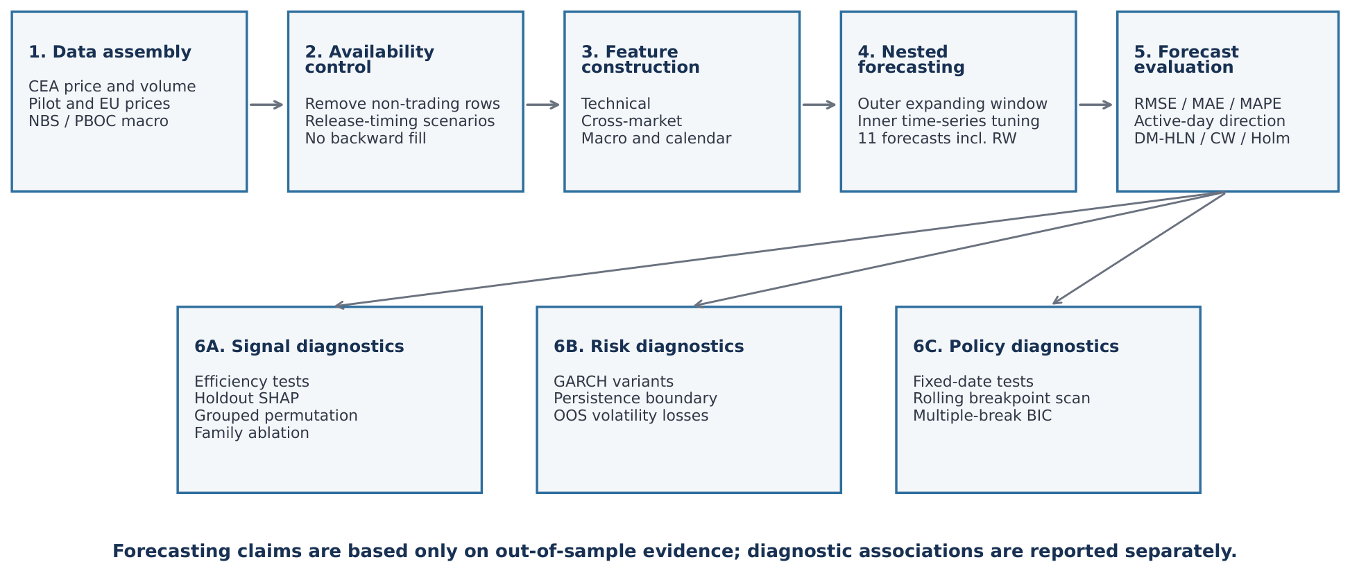
The scientific contribution is fourfold. First, the forecasting tournament uses a common expanding outer window and a nested expanding inner window for hyperparameter selection, so model comparisons do not depend on default settings or unequal training spans. Second, formal efficiency tests are reported alongside forecasting tests, revealing that statistical dependence can coexist with a failure to obtain lower out-of-sample price error. Third, model-output attribution is separated from predictive evidence through an untouched interpretation holdout and out-of-sample feature-family ablation. A common-sample energy/weather sensitivity and a two-by-two decomposition of macro release timing and first-public values test two information-set concerns without overwriting the original 26-variable tournament. Fourth, fixed-date tests are complemented by rolling and BIC-selected multiple-break diagnostics, while volatility specifications are compared using both full-sample information criteria and common-sample one-step-ahead losses. Figure 1 presents the six-stage system and separates forecasting from signal, risk and policy diagnostics.

2. Related Work and Positioning

2.1. Carbon-Price Behavior, Correlates and Forecasting

Early EU ETS research identifies energy prices, macroeconomic conditions and allocation events as correlates of allowance prices and documents structural instability [4,5,6]. Its limitation for the present question is external validity: the mature EU market has a longer history, different participation rules and deeper liquidity than China’s national market. Adekoya [7] shows that energy-price information can assist allowance-price prediction, but an energy-price predictor that is informative in a developed market need not remain informative in a thin Chinese daily series.

China-specific evidence makes that transfer problem concrete. The national system began with output- and benchmark-linked free allocation in the power sector rather than a fixed mass cap. Within the structural model of Goulder et al. [15], this design alters simulated abatement and price incentives. Pilot-market studies report heterogeneous associations with energy, industry, financial and sentiment variables across Beijing, Guangdong, Hubei and Shenzhen [16,17,18]. Separate simulation work estimates equilibrium-price responses under assumed coverage and allocation settings [19]. For the national market, Liao et al. [20] attribute more explained variation to own-price history and trading activity than to international or broad macroeconomic variables. That study is informative about model association through August 2024, but it does not test nested out-of-sample forecast gains or the 2025 sector expansion. The literature therefore motivates testing market-specific predictors without treating those rationales as transmission mechanisms identified by the present design.

A complementary literature examines low-carbon outcomes of policy and market design rather than short-horizon allowance-price behavior. Du et al. [21] evaluate ecological efficiency across Chinese cities and report that low-carbon pilot-city policy improves efficiency through green technology innovation. Shao et al. [22] use a spatial difference-in-differences design to study pollution co-governance under China’s pilot ETS, whereas Zhu et al. [23] use an agent-based model to examine heterogeneous firms’ adoption and diffusion of low-carbon technologies within an ETS. These studies establish why a credible carbon-price signal matters for urban environmental performance and firm investment, but their outcomes, horizons and inferential designs differ from ours. They analyze city-level policy effects or simulated firm-level adoption over multi-period transitions; the present study evaluates a traded national CEA price one session ahead and makes no causal claim about policy or technology mechanisms. The literature is therefore complementary: low-carbon-development studies motivate the economic relevance of the price signal, while our analysis tests whether that daily signal can be forecast reliably beyond a no-change benchmark.

Hybrid ARIMA–least-squares support-vector methods and explainable machine learning models report strong carbon-price accuracy [8,9]. These studies establish that nonlinear learners can fit carbon-price dynamics, but reported results remain difficult to compare when markets, targets, horizons, benchmarks and validation schemes differ. In particular, a low error relative to another fitted model does not establish incremental value relative to the no-change price forecast. The more recent allowance-cap study of Wang et al. [10] combines structural variable screening and supervised learning, but forecasts a policy-determined aggregate cap rather than a traded daily allowance price. Our target, information set and economic interpretation are therefore different.

The China-specific gap has three parts. First, post-2025 evidence is short, so a coverage expansion must be treated as a candidate break rather than assumed to have shifted the price process. Second, technical, cross-market and low-frequency macro variables carry different information and should be tested both jointly and by family. Third, a high share of flat-price days can coexist with serial dependence and short-horizon mean reversion without creating a forecast advantage after genuine time ordering. The present study addresses these gaps with a common benchmark, nested expanding validation, formal efficiency tests and separate model-association, prediction, volatility and structural-stability analyses.

2.2. Machine Learning, Interpretability and Forecasting Discipline

Regularized linear models, nearest-neighbor methods, kernel machines and tree ensembles have complementary inductive biases: shrinkage controls collinearity [24,25,26], kernels and neighbors capture local nonlinearity [27,28], and bagged or boosted trees model interactions [29,30]. Neural networks are flexible but data-hungry [31,32]; on short financial series, their additional variance can outweigh any reduction in bias [33,34].

The central limitation of algorithm tournaments is evaluation design. Random cross-validation leaks future regimes into training; untuned defaults can disadvantage some learners; unequal rolling and expanding windows confound model class with information-set size; and testing many forecasts inflates false discoveries [11,12,14,35]. We therefore use a nested expanding-window protocol, a common outer information set, the Harvey–Leybourne–Newbold small-sample correction to Diebold–Mariano statistics, Clark–West tests and Holm adjustment across model comparisons [13,36,37].

Interpretability is a separate inferential task. SHAP and partial dependence describe a fitted response surface but do not establish economic causation or guarantee out-of-sample stability [38,39]. To avoid “interpretability washing”, this study fits the interpretation forest only on the first 75% of the sample, computes SHAP and permutation evidence on the untouched final quarter, and corroborates the rankings with an out-of-sample family ablation. The language throughout is consequently “model-output attribution”, “model-specific association” or “incremental predictive content”. Even on that untouched holdout, SHAP remains conditional on the fitted forest and the chosen sample split: it describes model-associational patterns, not causal drivers, invariant out-of-sample effects or exploitable forecasting signals.

2.3. Market Efficiency and Volatility

Weak-form efficiency concerns information contained in the price’s own history; broader public-information efficiency also concerns macroeconomic and inter-market variables [40,41]. A random-walk forecasting benchmark alone is insufficient to prove either form. We therefore combine forecast comparison with Ljung–Box autocorrelation, sign runs, Lo–MacKinlay variance-ratio and BDS nonlinear-dependence tests. The technical-only ablation is the closest test of weak-form predictability, whereas the full feature set asks the broader public-information forecasting question.

Conditional-mean predictability must also be separated from conditional-variance predictability. ARCH/GARCH models allow volatility clustering, Student’s t errors allow heavy tails, EGARCH and GJR-GARCH allow asymmetric dynamics, and IGARCH represents a unit-persistence boundary [42,43,44]. Because a persistence estimate of one cannot support a finite half-life, we explicitly test whether persistence is below unity and compare alternative volatility specifications before drawing risk-management implications.

2.4. Analytical Framework and Hypotheses

The analysis is organized around four pre-specified propositions. H1₀ (forecast benchmark null): no tested model reduces out-of-sample price loss relative to the random walk. Failure to reject H1₀ is evidence of no demonstrated incremental forecast value, not proof of market efficiency. Formal serial-dependence tests provide complementary evidence. H2 (conditional feature-family ordering): technical features receive greater model attribution and out-of-sample predictive content within the 26-variable baseline than the cross-market, macroeconomic or calendar/regime families; a separate common-sample energy/weather sensitivity tests whether that ordering persists after adding the available fundamental measures. H2 remains logically compatible with H1₀: a family may rank first within a model yet still be too weak or unstable to beat the benchmark. H3a (volatility persistence): conditional CEA volatility is highly persistent; the unit-persistence boundary is tested rather than assumed away. H3b (expansion-period structural-change hypothesis): the conditional mean and/or conditional variance displays a break around the March 2025 expansion period. H3b is examined with fixed-date, rolling, multiple-break and variance-equation diagnostics; none identifies a causal policy parameter.

3. Data

3.1. Sources and Coverage

The dependent variable is the daily closing CEA price on the SEEE. The CEA, cross-market and final-history macroeconomic series were accessed through the proprietary Wind Financial Terminal (Wind Information Co., Ltd., Shanghai, China); the underlying institutions are identified in

Table 1. Data sources, frequencies and forecasting roles.

Data Block	Content/Frequency	Source	Availability Treatment and Role
National CEA	Daily open, high, low, close, volume and turnover	Wind Financial Terminal; underlying venue SEEE [45]	Same-day public market information; target and technical features
Regional pilots/EU	Daily closing prices	Wind Financial Terminal; official trading venues	Available after the respective day-t venue closes and before the next CEA session; short aligned gaps forward-filled
PPI and CPI	Monthly year-on-year rates	Wind final history; official NBS first releases [46,47]	Legacy 15-day/final-history baseline; actual timestamp and first-public rate in the real-time sensitivity
M0 and RMB loan balance	Monthly levels and year-on-year rates	Wind final history; official PBOC first releases [48,49]	Baseline growth from final levels; actual timestamp and officially reported first-public growth in the real-time sensitivity
Weather sensitivity	Daily HDD18, CDD18 and 2 m temperature range	NOAA/NCEP GFS 0.5-degree forecasts [50,51]	Archived forecast fields verified as available before the target CEA session; not realized weather
Public coal sensitivity	Ten-day Shanxi Blend (5500 kcal) circulation-market price, CNY/t	National Bureau of Statistics [47]	Last published level carried forward only after its displayed release time; not a daily delivered fuel cost
Generation sensitivity	Estimated total national electricity generation, GWh/day	CarbonMonitor-Power [52,53]	Assumed 21-calendar-day availability lag and 28-day check; generation proxy, not observed load
Restricted coal alternative	Daily Qinhuangdao Q5500 price, CNY/t	Wind Financial Terminal	One additional CEA-session lag; used only as a proprietary robustness measure because historical publication timestamps are unavailable

. After removing 82 vendor rows with zero closing prices that represent non-trading sessions, the price sample contains 1203 genuine trading days from 16 July 2021 to 6 July 2026 and yields 1202 next-day returns. Cross-market context comprises Hubei, Guangdong, Shanghai and Shenzhen pilot-market prices and the European carbon price. The baseline retains PPI, CPI, M0 and RMB loan-balance growth as its four macroeconomic inputs. Official NBS and PBOC monthly releases provide the publication timestamps and first-public year-on-year rates used in the real-time sensitivity. The weather and energy measures enter only the separately reported sensitivity.

Predictor eligibility requires continuous comparison-period coverage, a documented measurement scope and a reproducible availability rule. The public sensitivity meets these conditions for pre-open GFS forecasts and the NBS ten-day coal measure. CarbonMonitor-Power supplies a constructed national generation series rather than load and does not retain observation-specific historical release timestamps; its 21- and 28-day availability rules are therefore explicitly sensitivity assumptions. The cited NEA public materials provide monthly electricity statistics and selected peak-load announcements, but they do not provide a continuous, downloadable national daily observed-load series with historical availability timestamps suitable for this design [54,55]. The restricted wind coal alternative supplies daily observations but not a historical publication-time field. Accordingly, the augmented exercise tests whether the baseline ordering changes under these measured additions; it does not claim complete observation of daily fuel cost or electricity demand.

No personal, household or respondent-level records are used, so individual anonymization is not applicable. The redistribution safeguard is instead aggregation and removal of vendor-schema information. Appendix A contains only 28 rows of aggregate descriptive statistics under analytical variable labels. It excludes date-indexed or row-level wind observations, terminal instrument codes, vendor field identifiers, retrieval metadata and local file paths. No processed daily panel or daily prediction file capable of reconstructing the proprietary records is supplied.

3.2. Feature Engineering

The main tournament uses 26 predictors in four families.

Table 2. Baseline predictor families and separately tested energy/weather sensitivity variables. Predictive rationales are not causally identified.

Family	Features	Predictive Rationale (Not Causally Identified)
Technical: return/price (9)	Lagged returns (1, 2, 3, 5 days); moving-average gaps (5, 10, 20); momentum (5, 10)	Proxies for reversal, continuation and deviation from recent reference prices
Technical: trading/risk (6)	Realized volatility (5, 10, 20); daily high–low range; log volume; volume anomaly	Proxies for trading intensity, concentration and short-horizon uncertainty
Cross-market: EU (2)	EU return; EU 20-day standardized price gap	Possible shared exposure to fossil-fuel, macroeconomic and climate-policy news; direct comparability is limited by separate products and institutions
Cross-market: Chinese pilots (2)	Pilot-average return; CEA-to-pilot price gap	Possible shared domestic information, qualified by different regional coverage, allocation, participation and liquidity
Macro: prices/activity (2)	PPI and CPI inflation	Public proxies for industrial input prices and aggregate-demand conditions
Macro: money/credit (2)	M0 growth; loan-balance growth	Public proxies for monetary and financing conditions
Calendar/regime (3)	Weekday; December compliance indicator; post-expansion indicator	Calendar and post-period indicators without a policy interpretation
Sensitivity only: energy/weather (5)	GFS HDD18, CDD18 and daily temperature range; last-published coal-price level; lagged national generation estimate	Forecast-available temperature, fuel-price and power-system-activity measures; the coal and generation variables retain their published measurement scope

lists their operational definitions and the five variables used only in the public energy/weather sensitivity; Appendix B (

Table A2. Descriptive statistics for the exact-release macroeconomic and energy/weather sensitivity variables.

Variable	Unit	N	Mean	SD	Min	Median	Max
Exact-first PPI YoY	percentage points	1202	0.573	5.021	$-5.400$	$-1.900$	13.50
Exact-first CPI YoY	percentage points	1202	0.737	0.903	$-0.800$	0.550	2.800
Exact-first M0 YoY	%	1202	10.97	2.840	2.700	11.50	18.50
Exact-first RMB-loan YoY	%	1202	9.530	2.136	5.500	10.80	12.30
GFS HDD18	degree-days	1202	11.18	7.964	1.499	9.229	28.12
GFS CDD18	degree-days	1202	1.711	1.975	0.000	0.635	6.685
GFS daily temperature range	degrees C	1202	8.499	0.995	5.976	8.509	11.64
NBS Shanxi Blend 5500	CNY/t	1202	954.97	243.77	618.00	877.90	1820.6
Wind Q5500 alternative, lagged	CNY/t	1201	932.32	224.13	609.00	866.00	1704.5
Generation proxy, 21-day rule	GWh/day	1202	25,931.3	2960.5	17,530.4	25,706.4	34,376.3

) reports aggregate descriptive statistics for the added and exact-release variables. Technical variables proxy return memory, relative prices, trading activity and uncertainty. EU and pilot variables may co-move with the national CEA series because the markets can share public news, although separate compliance products and institutional differences limit direct comparability. Macro and calendar variables are public-information proxies. The sensitivity adds three forecast-weather measures, one last-published coal-price level and one conservatively lagged generation estimate; a restricted specification replaces the public ten-day coal measure with the one-session-lagged daily wind alternative. These rationales motivate inclusion; the design tests predictive association and does not identify economic transmission.

3.3. Descriptive Statistics

Table 3. Descriptive statistics for representative target and predictor variables; the full predictor table is reported in Appendix A (Table A1).

Variable	n	Mean	Std. Dev.	Min	Max	Skew/Kurt.
CEA close (CNY/t)	1202	70.223	16.272	41.460	105.650	0.37/$-0.86$
Next-day log return	1202	0.00043	0.01785	$-0.10399$	0.09388	0.27/6.83
5-day MA gap	1198	0.00082	0.01803	$-0.08219$	0.11426	0.84/5.09
Daily range	1202	0.01653	0.02437	0.00000	0.18841	2.47/7.86
EU return	1159	0.00026	0.02906	$-0.28589$	0.33863	0.24/27.72
Pilot-average return	1198	0.00010	0.04089	$-0.27183$	0.28228	0.29/19.91
PPI inflation (%)	1191	0.513	4.997	$-5.400$	13.500	1.22/0.10
M0 annual growth	961	0.115	0.022	0.027	0.172	$-0.91$/3.49

expands the descriptive summary to representative variables from every family and adds skewness and excess kurtosis; complete statistics for all 26 predictors are reported in Appendix A (

Table A1. Full descriptive statistics for the 26 predictors, the next-day return target and the CEA closing price. Statistics are calculated before model-fold imputation; SD is the sample standard deviation and excess kurtosis uses the Fisher definition.

Variable	Code	Family	N	Mean	SD	Min.	Median	Max.	Skew.	Ex. Kurt.
CEA log return, lag 1 trading day	ret_lag1	Technical	1200	0.000420	0.017866	$-0.103990$	0.000000	0.093880	0.273200	6.818611
CEA log return, lag 2 trading days	ret_lag2	Technical	1199	0.000411	0.017870	$-0.103990$	0.000000	0.093880	0.274506	6.816538
CEA log return, lag 3 trading days	ret_lag3	Technical	1198	0.000406	0.017877	$-0.103990$	0.000000	0.093880	0.275280	6.810712
CEA log return, lag 5 trading days	ret_lag5	Technical	1196	0.000405	0.017892	$-0.103990$	0.000000	0.093880	0.275328	6.794682
CEA 5-day moving-average gap	ma_ratio5	Technical	1198	0.000824	0.018027	$-0.082189$	0.000000	0.114259	0.837764	5.093685
CEA 10-day moving-average gap	ma_ratio10	Technical	1193	0.001818	0.028263	$-0.090090$	$-0.000373$	0.154317	0.985712	3.934180
CEA 20-day moving-average gap	ma_ratio20	Technical	1183	0.003901	0.044968	$-0.133593$	$-0.000045$	0.233329	0.979123	3.328758
CEA 5-day momentum	mom5	Technical	1197	0.002575	0.036948	$-0.112863$	0.000000	0.196702	1.030048	3.823201
CEA 10-day momentum	mom10	Technical	1192	0.005197	0.056194	$-0.165000$	0.000000	0.315374	1.275433	4.483926
CEA 5-day realized volatility	rvol5	Technical	1197	0.013489	0.012294	0.000000	0.010160	0.075953	1.921805	4.813871
CEA 10-day realized volatility	rvol10	Technical	1192	0.014364	0.010727	0.000000	0.011879	0.061318	1.458620	2.406397
CEA 20-day realized volatility	rvol20	Technical	1182	0.014998	0.009403	0.001538	0.012979	0.045643	1.013143	0.561530
CEA daily high-low range divided by close	range	Technical	1202	0.016528	0.024367	0.000000	0.007180	0.188406	2.467984	7.857367
Log CEA trading volume	logvol	Technical	1202	10.761060	3.878200	0.000000	12.201075	16.835005	$-0.982593$	$-0.103152$
CEA 20-day volume anomaly (z-score)	vol_z	Technical	1183	0.101252	1.087402	$-1.929294$	$-0.326573$	4.246313	1.411423	1.590694
EU allowance log return	eu_ret1	Cross-market	1159	0.000257	0.029064	$-0.285888$	$-0.000161$	0.338632	0.241437	27.715489
EU allowance 20-day price anomaly (z-score)	eu_gap	Cross-market	1141	0.136671	1.281607	$-3.643017$	0.255697	3.095586	$-0.146614$	$-0.699665$
Pilot-average allowance log return	pilot_ret1	Cross-market	1198	0.000096	0.040892	$-0.271827$	0.000000	0.282280	0.293551	19.907841
CEA-to-pilot-average price gap	pilot_gap	Cross-market	1199	0.397237	0.363496	$-0.189053$	0.346696	1.523157	0.358585	$-0.787582$
Producer price inflation (year-on-year, %)	ppi_yoy	Macro-financial	1191	0.513182	4.996530	$-5.400000$	$-1.900000$	13.500000	1.215449	0.098165
Consumer price inflation (year-on-year, %)	cpi_yoy	Macro-financial	1191	0.727456	0.905433	$-0.800000$	0.500000	2.800000	0.630683	$-0.505720$
M0 annual growth	m0_yoy	Macro-financial	961	0.114925	0.021797	0.027304	0.116593	0.171797	$-0.906675$	3.493783
Loan-balance annual growth	loan_yoy	Macro-financial	961	0.091082	0.021720	0.055196	0.093175	0.121558	$-0.105216$	$-1.532049$
Day of week (Monday = 0)	dow	Calendar/regime	1202	2.009983	1.407095	0.000000	2.000000	4.000000	$-0.008747$	$-1.288292$
December indicator	is_dec	Calendar/regime	1202	0.092346	0.289634	0.000000	0.000000	1.000000	2.819647	5.960322
Post-expansion indicator	post_expansion	Calendar/regime	1202	0.257072	0.437201	0.000000	0.000000	1.000000	1.113141	$-0.762187$
Next-day CEA log return target	y	Target	1202	0.000433	0.017854	$-0.103990$	0.000000	0.093880	0.271287	6.827468
CEA closing price (CNY/t)	close	Target/context	1202	70.223145	16.271875	41.460000	69.355000	105.650000	0.371160	$-0.855254$

). The CEA price averages 70.22 CNY/t. Next-day returns have a mean of 0.043%, standard deviation of 1.785%, positive skewness of 0.27 and excess kurtosis of 6.83. High kurtosis in CEA, EU and pilot returns supports heavy-tailed volatility models and cautions against Gaussian break inference.

The descriptive predictor tables use 1202 model-ready forecast-origin rows because the last of the 1203 observed prices has no subsequent trading-day target.

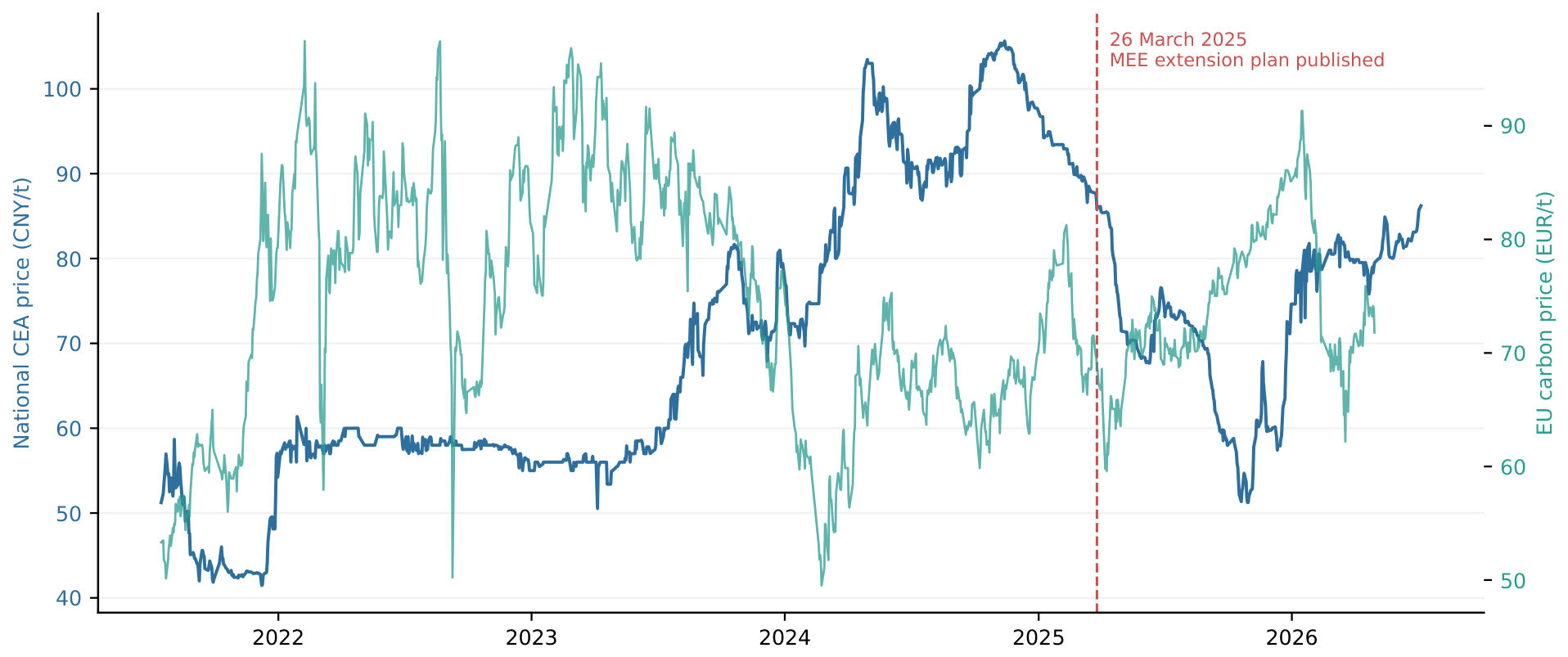
Figure 2 provides the corresponding national and European price paths and marks the pre-specified expansion date.

4. Methods

The empirical design is predictive rather than causal. Unlike city-panel difference-in-differences designs used to estimate low-carbon policy effects [21,22], or the agent-based simulation used to characterize technology-adoption equilibria [23], this study estimates neither a treatment effect nor a structural adoption mechanism. It asks whether information available at each forecast origin reduces one-step-ahead national CEA price loss relative to the no-change benchmark, with preprocessing and hyperparameter selection confined to expanding training windows. Accordingly, the adjacent low-carbon literature motivates the relevance of the price signal, but it does not convert the present feature attributions into causal mechanisms.

4.1. Data Cleaning, Alignment and Leakage Control

Zero-price vendor rows are removed before returns are calculated. Cross-market series are aligned to the national CEA calendar and short gaps are forward-filled for at most five consecutive observations on the combined market-date index. Missing values are retained and median-imputed separately inside each training window. The original 26-variable pipeline detects each final-history monthly update, computes M0 and loan growth from levels 12 reference months apart, applies a 15-calendar-day embargo and then carries the value forward on the CEA calendar. This fixed-delay/final-history construction is retained as the legacy comparator.

The real-time macro sensitivity matches CPI, PPI, M0 and RMB loan balance to 296 official NBS and PBOC releases from June 2020 to July 2026, including all 240 expected records in the July 2021–June 2026 core window [47,49]. Each record retains its Beijing publication timestamp and the year-on-year rate reported when first released; PBOC identifies the current-period figures as preliminary. A value is eligible only when its timestamp is strictly earlier than the target session’s 09:30 Beijing opening, so an NBS release stamped at 09:30 first enters the next eligible session. The analysis crosses the legacy versus exact timing rules with final-history versus first-public values, producing four cells, and adds a macro-omitted boundary. This separates timing from value-vintage effects. It is an official first-release reconstruction, not an archive of every later revision state.

Monthly macro releases necessarily enter the daily panel as step functions: carrying the latest eligible release forward does not create a new daily observation, but records the information actually available before each session. This persistence means that macro coefficients or attributions must not be interpreted as high-frequency measurements. We address the concern in three ways. First, the macro-omitted boundary and the exact-release/first-public specification are evaluated on the same 952 targets. Second, the already-produced one-step daily price forecasts and realized prices are averaged within target weeks and months; these are lower-frequency summaries, not newly fitted direct weekly or monthly models. Third, flat-price diagnostics compare release-update and non-update days, stratify model errors between flat and active targets, and use dependence-robust and circular-shift checks for associations between carried macro levels and the flat-day indicator.

For target session T, the weather sensitivity uses the preceding calendar day’s GFS 00Z cycle and eight f018–f039 2 m temperature forecasts. All source objects were available before the target opening. A fixed China land mask and latitude weights produce HDD18, CDD18 and the daily temperature range; full-day realized weather is not used. The public coal feature is the most recent NBS Shanxi Blend (5500 kcal) price whose displayed 09:30 release precedes the target opening; no value is interpolated or back-filled. A restricted alternative uses the Wind Qinhuangdao Q5500 series with one additional CEA-session lag, but is not labeled point-in-time verified. The generation feature uses the latest CarbonMonitor-Power observation satisfying an assumed 21-calendar-day availability rule, repeated at 28 days; it remains a generation proxy rather than observed load. All comparisons retain the same 952 origins, target prices and returns. Each random-forest specification is tuned only within its expanding training windows; leave-family-out comparisons reuse the relevant full model’s block-specific settings. Only aggregate results are reported, and row-level wind-derived observations are not distributed.

4.2. Forecasting Target and Expanding-Window Tournament

Let $P_t$ be the CEA closing price on trading day t. The forecasting target is the next-day logarithmic return in Equation (1),

$$r_{t+1}=\ln \left(P_{t+1}/P_t\right),$$

(1)

which is predicted from the day-t feature vector ${\mathbf{x}}_t$. The forecast information cutoff is after all day-t market closes used in the feature vector, including the European series, and before the next CEA session opens; no result assumes execution at $P_t$. A price forecast is reconstructed as ${\widehat{P}}_{t+1}=P_t\exp \left({\widehat{r}}_{t+1}\right)$. The first 250 observations initialize the outer expanding window; models are refitted every 60 trading days, leaving 952 forecasts with target dates from 29 July 2022 through 6 July 2026. At every outer refit, hyperparameters are selected only from the available training observations using a three-split expanding inner validation. All learners, including SVR, receive the same expanding information set. This nested rolling-origin design prevents random-fold leakage and separates parameter selection from the outer test period [11,12].

Eleven forecasts are compared: a random-walk return of zero, ARIMA(1,0,1), ridge, lasso, elastic net, k-nearest neighbors, SVR, random forest, histogram gradient boosting, a small multilayer perceptron and an unweighted machine learning ensemble.

Table 4. Nested expanding-window hyperparameter grids. No outer-test observation enters tuning or preprocessing.

Model	Configuration
Random walk/ARIMA	zero return; ARIMA order (1,0,1), both under the outer expanding window
Ridge/lasso	$\alpha \in \{0.1,1,10\}$; $\alpha \in \{{10}^{-4},5\times {10}^{-4},{10}^{-3}\}$
Elastic net	$\alpha \in \{5\times {10}^{-4},{10}^{-3}\}$; mixing $\in \{0.25,0.75\}$
k-nearest neighbors	$k\in \{5,10,20\}$
Support-vector regression	radial basis; $C\in \{0.1,1\}$; $\epsilon \in \{0.002,0.01\}$
Random forest	160 trees; depth $\in \{4,7\}$; minimum leaf $\in \{3,8\}$
Gradient boosting	depth $\in \{2,3\}$; learning rate $\in \{0.03,0.07\}$; 200 iterations
Neural network	hidden units $\in \{4,8\}$; $L_2\in \{10,100\}$; learning rate $\in \{0.0003,0.001\}$; tolerance ${10}^{-6}$; 2000 iterations
Ensemble	unweighted mean of the eight nested-tuned machine learning forecasts

reports the deliberately small inner grids. Restricting the grids controls the variance and computational burden of tuning on roughly one thousand observations. All preprocessing—imputation and, where applicable, standardization—is fitted inside each training fold. Implementations use scikit-learn [56]. Before price reconstruction and ensemble averaging, forecasts from the eight machine learning models are clipped to the common fixed interval $[-0.11,0.11]$ in logarithmic-return units; the random-walk and ARIMA benchmarks are not clipped.

An initial MLP diagnostic grid selected its upper $L_2$ boundary in every refit block and produced many clipped forecasts. The main tournament therefore uses the pre-specified combined stabilized grid in Table 4, selected exclusively inside the same three-split expanding inner windows. A diagnostic ablation on the identical 952 outer origins retains the initial grid and changes convergence tolerance, $L_2$ strength, learning rate and width in separate arms before combining them; a compact L-BFGS arm checks optimizer dependence. We report inner loss, outer error, selected settings, iterations, convergence warnings and the frequency of forecasts reaching the common $\pm 11\%$ clipping bound. No arm is chosen by outer-test performance. The ensemble and all benchmark-comparison statistics use the stabilized main-tournament MLP forecast.

4.3. Evaluation

Price accuracy is measured by RMSE, MAE and MAPE; sign accuracy is reported on all days and on active days with non-zero realized returns. For each model, both the squared-price-loss and squared-return-loss differentials against the random walk are evaluated by Diebold–Mariano statistics with the Harvey–Leybourne–Newbold finite-sample factor [57]. Holm-adjusted p-values address the ten simultaneous benchmark comparisons separately for each loss definition. Clark–West one-sided tests are also reported because a zero-return forecast is nested in return models [13,36,37]. For $e_{m,t}={\widehat{P}}_{m,t+1}-P_{t+1}$ and $d_t=e_{m,t}^2-e_{0,t}^2$, the unadjusted statistic is defined in Equation (2):

$$\mathrm{DM}=\overline{d}/\widehat{\mathrm{se}}\left(\overline{d}\right),$$

(2)

Here, $\overline{d}$ is the sample mean loss differential and $\widehat{\mathrm{se}}\left(\overline{d}\right)$ is its estimated standard error; the reported statistic applies the finite-sample factor. A positive statistic indicates higher loss than the random walk. Active-day directional accuracy is defined in Equation (3), where $\mathcal{A}=\{t:|r_{t+1}|>0\}$:

$$\mathrm{DA}={\displaystyle \frac{1}{\left|\mathcal{A}\right|}}\sum _{t\in \mathcal{A}}\mathbf{1}\left[\mathrm{sign}\left({\widehat{r}}_{t+1}\right)=\mathrm{sign}\left(r_{t+1}\right)\right].$$

(3)

Directional accuracy is a descriptive forecast metric only. No model is selected from this ranking to generate trading positions, and the study reports no economic-value backtest.

4.4. Interpretability

A separate random forest is trained on the first 75% of observations only. Mean absolute SHAP values, individual permutation importance and grouped family permutation are then computed on the untouched final 25%; partial-dependence profiles use the training sample [30,38,39]. The baseline expanding-window ablation compares the full 26-variable set, technical-only features and leave-one-baseline-family-out specifications. A separate public augmented ablation compares the exact-release 26-variable set with the full energy/weather specification, technical-only and without-technical variants, and leave-weather-, leave-coal- and leave-generation-out variants. Each ablation reuses the relevant full specification’s block-specific random-forest settings so that feature membership, rather than an unreported tuning change, drives the contrast. The macro two-by-two comparison uses the same holdout and grouped-permutation definition. These exercises describe model-specific associations and incremental predictive content; they do not establish economic causation. The holdout reduces sample reuse but does not establish that a SHAP ranking will remain stable in another period or translate into an exploitable forecasting signal.

4.5. Formal Efficiency Diagnostics

To avoid equating benchmark forecast failure with efficiency, we add four complementary diagnostics: Ljung–Box tests on daily returns at lags 5, 10 and 20; a sign-runs test on non-zero returns; heteroskedasticity-robust Lo–MacKinlay variance-ratio tests applied correctly to the log-price level at horizons 2, 5 and 10; and a BDS test on returns for nonlinear dependence [58,59]. Joint interpretation is required because the many flat-price days can induce dependence in return magnitudes while leaving non-zero return signs difficult to forecast.

4.6. Volatility and Structural Break

Conditional volatility is modeled with a GARCH(1,1) specification with Student’s t innovations in Equation (4),

$${\sigma }_t^2=\omega +\alpha {\epsilon }_{t-1}^2+\beta {\sigma }_{t-1}^2,$$

(4)

where ${\epsilon }_{t-1}$ is the return innovation, $\omega$ is the variance intercept, $\alpha$ measures the response to the previous squared innovation, $\beta$ measures conditional-variance persistence and $\alpha +\beta$ gives overall persistence [42,43]. A boundary diagnostic evaluates $H_0:\alpha +\beta =1$; GARCH-t is compared by AIC/BIC with restricted IGARCH-t, symmetric and asymmetric EGARCH-t, and GJR-GARCH-t. The information-criterion comparison is complemented by 702 one-step-ahead variance forecasts after a 500-observation initial window, with common 60-day refits and daily fixed-parameter recursion. As daily volatility is latent, absolute and squared daily returns are identified explicitly as noisy volatility and variance proxies; we report volatility RMSE/MAE, variance RMSE and QLIKE. Rankings are descriptive and are not followed by a significance test against an ex-post selected winner.

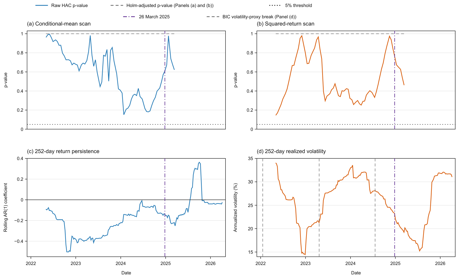
The fixed expansion date is 26 March 2025, when the MEE publicly released the sector-extension plan [2]. Fixed-date evidence comprises a Chow test on an AR(1) mean, HAC dummies in return and squared-return equations, CUSUM diagnostics and a Student’s t GARCH-X variance recursion. To reduce dependence on that date, an exploratory framework adds (i) candidate break dates every ten trading days after trimming 252 observations at each end, with Holm correction across the scan; (ii) 252-day rolling AR(1) and realized-volatility estimates updated every five trading days; and (iii) dynamic-programming BIC segmentation with at most three breaks and a pre-specified minimum segment of 180 trading days for the return AR(1) and log-squared-return level [4,60]. These diagnostics can locate gradual or differently timed instability but do not identify a causal expansion parameter.

An execution-calibrated economic-value backtest requires timestamped bid–ask quotes, depth, trades and a dated numerical fee schedule. The frozen dataset contains daily OHLC, volume and turnover. The cited public SEEE materials report daily aggregate market information [61]. The authenticated client displays best-five depth, transaction details and minute bars, but its user manual does not document a reproducible public historical export for those fields covering the study period [62,63]. Daily ranges cannot recover quoted spreads, effective spreads or execution slippage. Moreover, the national pricing notice establishes a government-guided fee-setting process but does not state a numerical national CEA rate [64]. The available data therefore support statistical forecast comparison, but not a market-calibrated execution simulation.

5. Results

5.1. Price Path and the 2025 Expansion

Figure 2 shows the national CEA price rising from about 51 CNY/t at launch to a peak near 105 CNY/t in late 2024, easing through 2025 and recovering to 86 CNY/t by mid-2026. The European series follows a different path, and its daily correlation with the CEA series is weak. These are descriptive phases; the turning points are not assigned to policy, compliance or market-maturation explanations because the present design does not identify their causes.

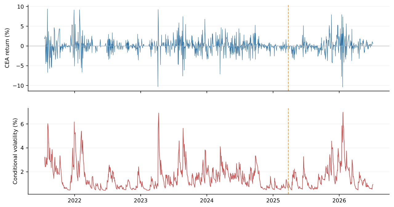
Figure 3 shows that periods of elevated returns and conditional volatility cluster in time, with quiet and turbulent intervals alternating. The figure is descriptive and does not by itself identify announcement or compliance-window effects.

5.2. The Forecasting Tournament: Is the Price Predictable?

Table 5. Nested expanding-window performance over 952 one-step-ahead forecasts. DM uses the HLN correction; Holm adjustment is applied separately to price- and return-loss comparisons.

Model	RMSE	Dir. Active (%)	Price DM p	Price Holm p	Return DM p	Return Holm p
Random walk	1.242	—	—	—	—	—
ARIMA	1.250	47.8	0.479	0.479	0.491	0.491
Neural network	1.251	50.4	0.036	0.109	0.145	0.290
Lasso	1.257	46.9	0.065	0.130	0.042	0.136
Elastic net	1.266	46.5	0.016	0.063	0.011	0.063
Ensemble	1.268	47.1	0.009	0.054	0.027	0.136
Random forest	1.289	47.4	0.009	0.054	0.031	0.136
Gradient boosting	1.314	44.8	<0.001	<0.001	<0.001	0.002
k-nearest neighbors	1.314	53.2	<0.001	<0.001	<0.001	<0.001
Ridge	1.335	49.6	<0.001	<0.001	<0.001	<0.001
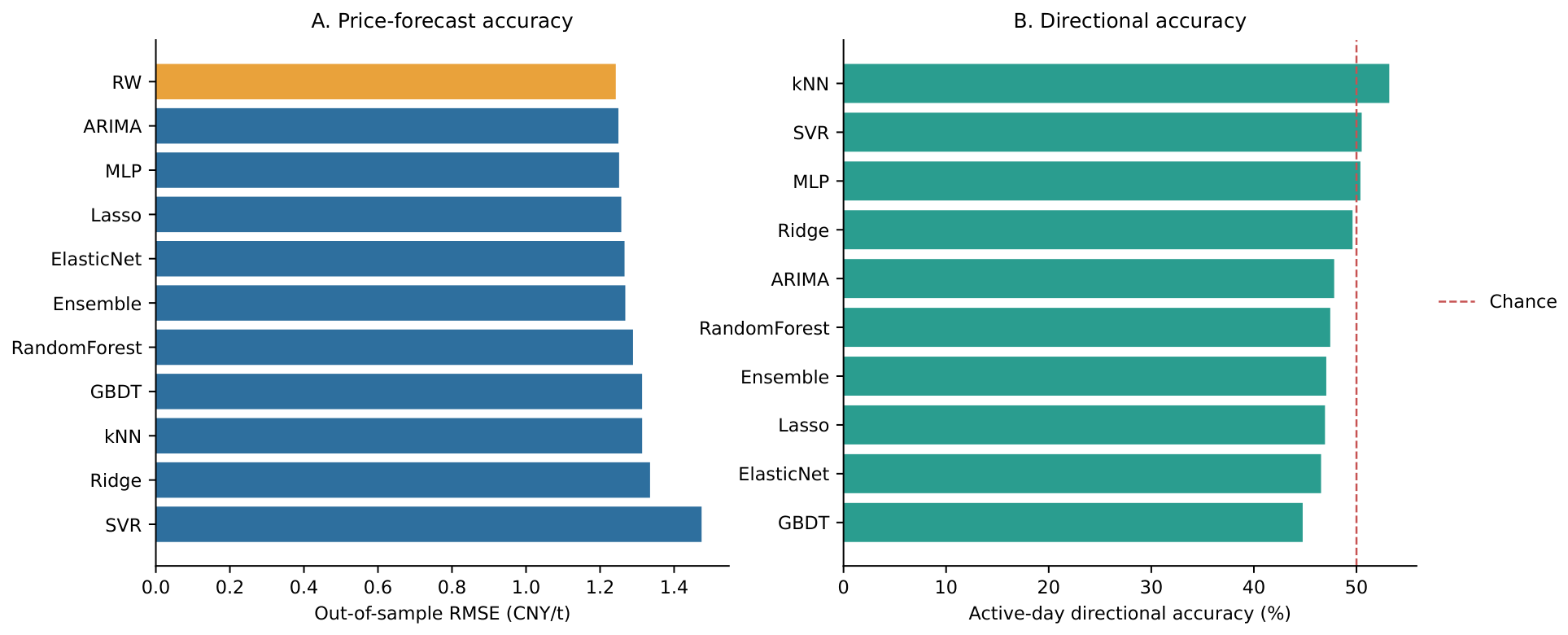
Support-vector regression	1.474	50.5	<0.001	<0.001	<0.001	<0.001

reports 952 outer-test forecasts after nested tuning and common expanding windows. The random walk retains the lowest RMSE (1.242 CNY/t) and MAPE (0.982%). ARIMA is closest (RMSE 1.250; price-loss DM $p=0.479$), followed by the stabilized MLP (1.251; $p=0.036$) and lasso (1.257; $p=0.065$). No model has a lower RMSE or a negative price- or return-loss differential relative to the random walk. After Holm adjustment, the price- and return-loss differentials remain non-significant at 5% for six models—ARIMA, the MLP, lasso, elastic net, random forest and the ensemble. The one-sided Clark–West test is nominally significant only for random forest ($p=0.033$), but its price RMSE is higher and its active-day direction is below 50%; this isolated metric is not interpreted as a stable gain.

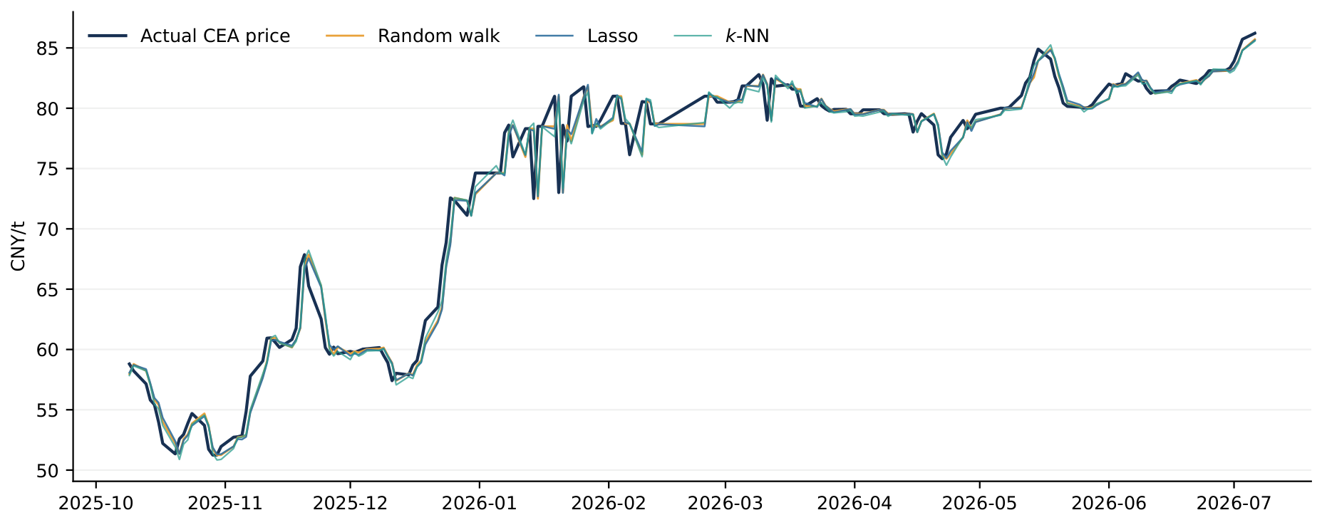
Active-day directional accuracy ranges from 44.8% to 53.2%, with k-nearest neighbors (k-NN) highest at 53.2%. The k-NN value is reported transparently as the numerical directional leader, but it is not used to select a trading strategy; its price RMSE is 1.314 CNY/t and its price- and return-loss differentials against the random walk remain significant in the unfavorable direction after Holm adjustment. These results support H1₀—no demonstrated reduction in out-of-sample price loss—but do not, by themselves, establish weak-form efficiency. In Figure 4, every model’s RMSE bar lies above the random-walk line, while the directional-accuracy panel clusters around 50%. Figure 5 shows that, over the final 180 trading days, both the random-walk and lasso paths mostly follow the lagged close and miss the magnitude of abrupt moves, so the fitted model adds little stable separation from the benchmark.

Table 6. MLP optimization and regularization diagnostics on the identical 952 outer-test origins. Warning counts cover all candidate-grid fits and final refits; the selected final fit did not reach its iteration cap in any block.

Specification	RMSE	MAE	Active Dir. (%)	Clipped n	Median Iter.	Warnings
Initial grid	3.848	2.918	50.0	79	133	0
Tight tolerance only	1.278	0.825	49.7	0	507	31
Strong $L_2$ only	1.246	0.745	46.7	0	110	0
Lower learning rate only	7.332	6.752	48.2	606	406	40
Compact width only	4.691	3.680	52.4	187	111	0
Combined stabilized Adam	1.251	0.773	50.4	0	960	195
Compact L-BFGS	1.247	0.749	47.8	0	29	0

reports the neural-network diagnostic results used to replace the unstable initial specification.

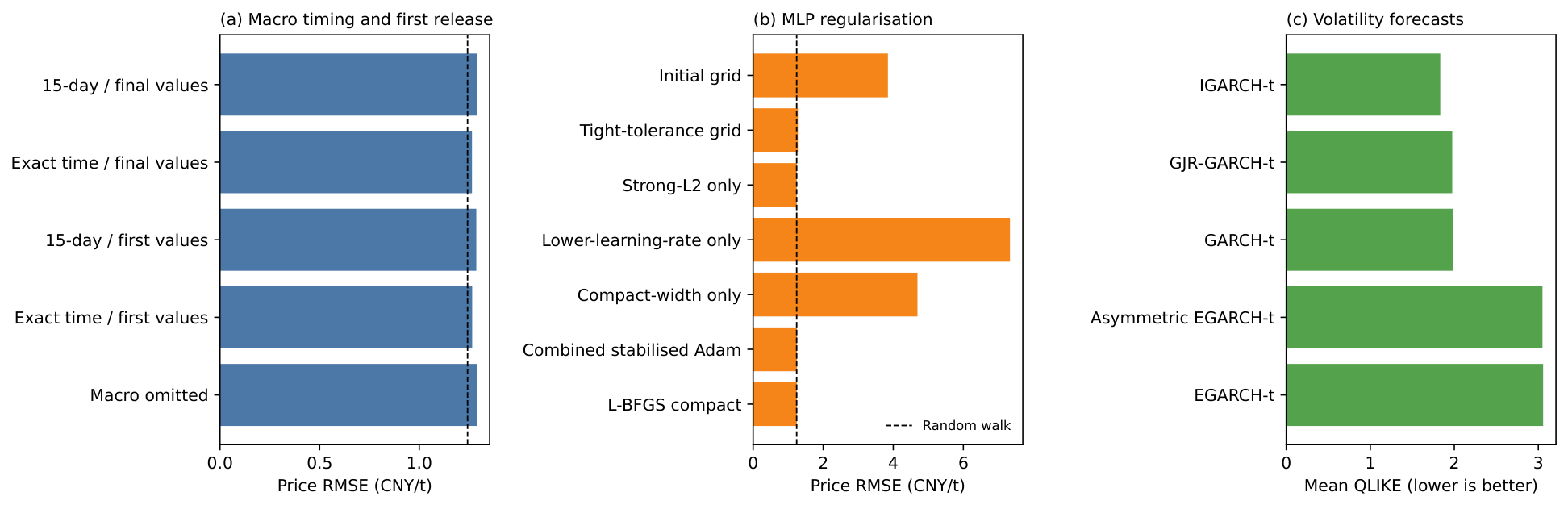
Table 6 identifies the initial MLP failure as an optimization-and-regularization problem rather than evidence that neural networks are intrinsically unsuitable. Its loose stopping tolerance terminates with extreme forecasts even though the selected $L_2=1$ is the upper boundary in all 16 refit blocks; 79 forecasts exceed the common clipping bound. Tightening the tolerance removes clipping and lowers RMSE to 1.278, while changing only $L_2$ to 10–100 lowers it to 1.246. Width or learning-rate changes alone do not stabilize the model. The pre-specified combined grid eliminates clipped forecasts and yields 1.251 CNY/t, but still does not beat the 1.242 random walk. Candidate-level convergence warnings in the larger grid are retained in the audit; every selected block fit completes before 2000 iterations.

5.3. Formal Efficiency Tests

Table 7. Formal efficiency diagnostics for daily CEA returns.

Test	Setting	Estimate	Statistic	p-Value
Ljung–Box	lags 5/10/20	—	22.53/42.17/49.81	<0.001/<0.001/<0.001
Runs test	non-zero return signs	—	0.484	0.628
Variance ratio	$q=2$/5/10	0.880/0.829/0.935	$-2.02$/$-1.51$/$-0.41$	0.043/0.131/0.684
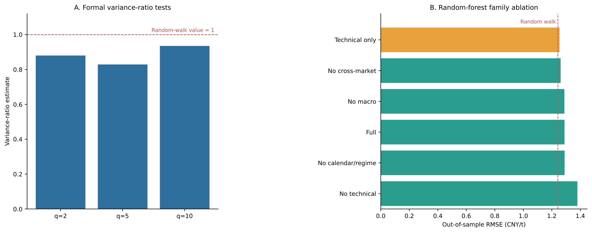
BDS	dimension 2	—	10.05	<0.001

prevents overinterpreting the forecast tournament. The sign-runs test does not reject independent non-zero directions ($p=0.628$), which accords with near-chance directional accuracy. All Ljung–Box tests reject no autocorrelation and BDS rejects independent and identically distributed returns. Correctly applied to log-price levels, the variance ratio is 0.880 at $q=2$ ($p=0.043$), providing weak short-horizon mean-reversion evidence, but the $q=5$ and $q=10$ ratios (0.829 and 0.935) are not significant. The diagnostics therefore reject a simple IID-return/random-walk characterization through autocorrelation and nonlinear-dependence evidence, but they do not support pervasive variance-ratio rejection across horizons. The forecasting result is narrower: the tested models do not convert the detected dependence into lower next-day price error.

5.4. Model-Specific Associations with Next-Day Returns

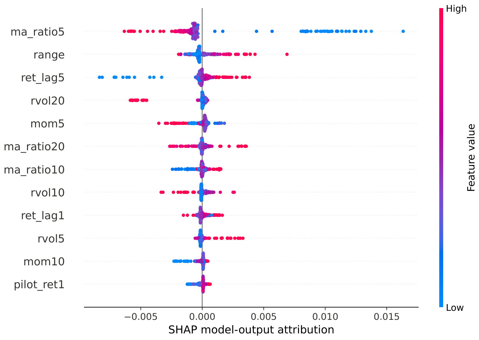
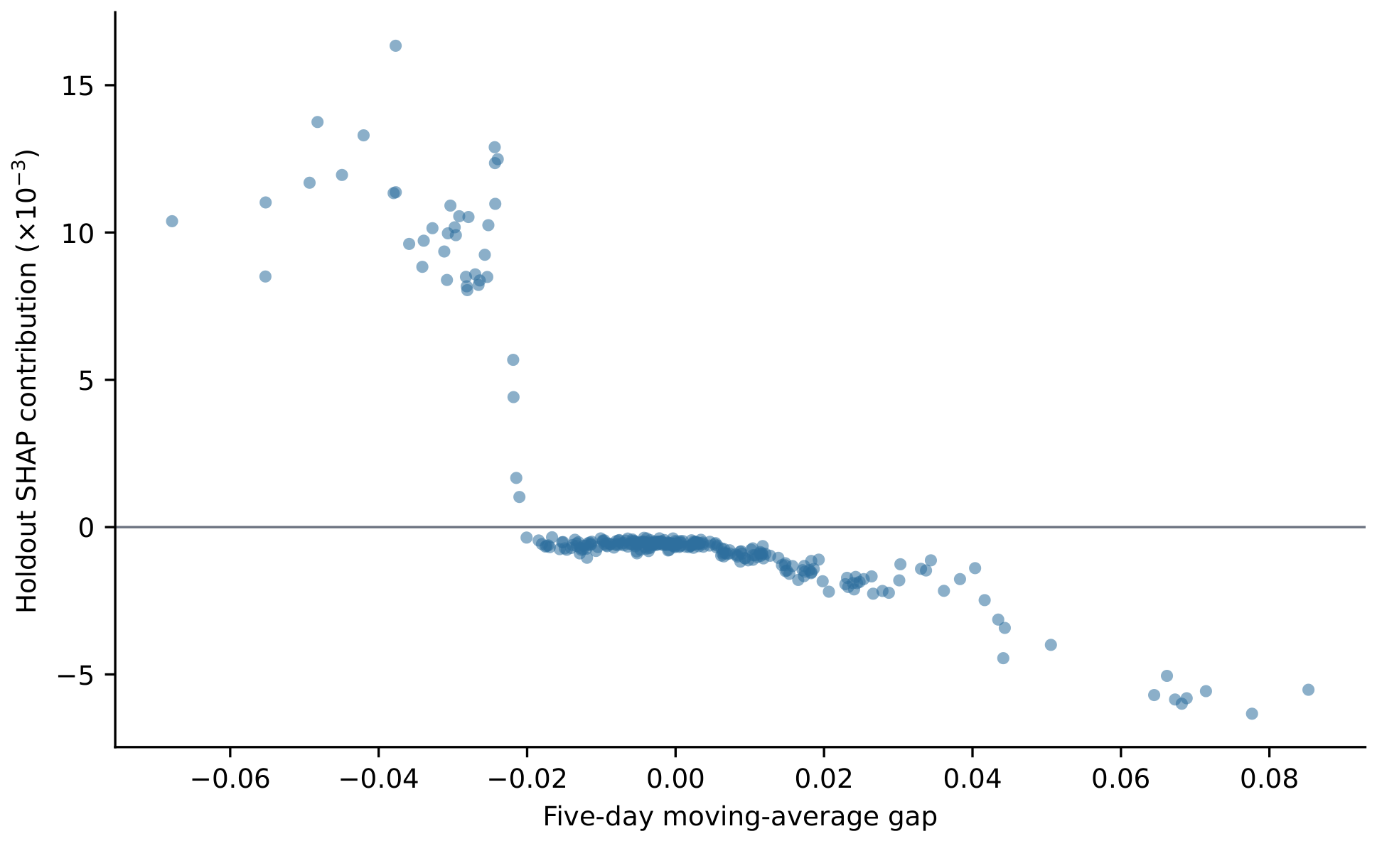
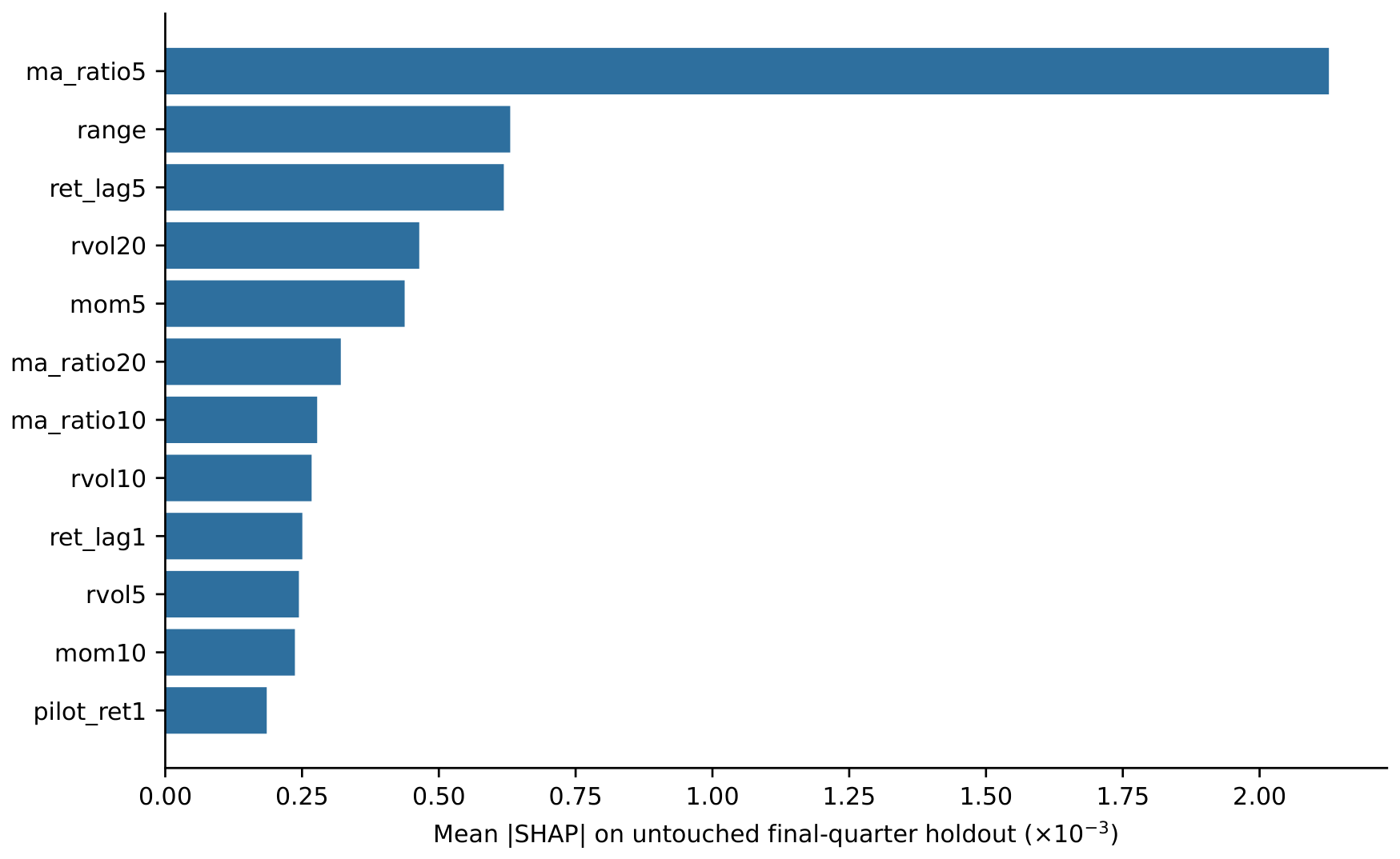
The interpretation forest is trained only through 7 April 2025 and evaluated on the untouched final quarter beginning 8 April 2025.

Table 8. Leading model-specific associations evaluated on an untouched final-quarter holdout.

Feature	Mean Absolute SHAP ($\times {\mathbf{10}}^{-\mathbf{3}}$)	Holdout Permutation Importance
5-day moving-average gap	2.127	0.0439
Daily high–low range	0.630	0.0426
5-day lagged return	0.619	0.0018
20-day realized volatility	0.464	$-0.0059$
5-day momentum	0.438	0.0020
20-day moving-average gap	0.321	$-0.0008$
10-day moving-average gap	0.278	0.0069

and Figure 6 show that the five-day moving-average gap, daily range and five-day lagged return have the largest holdout SHAP magnitudes. Figure 7 adds direction and dispersion: the same leading technical variables produce both positive and negative model-output attributions rather than a uniform monotonic model response. The moving-average gap and range also have positive individual permutation importance; several lower-ranked variables have zero or negative permutation importance, signaling instability rather than useful predictive content. These are model- and holdout-specific association patterns, not causal drivers or evidence that the ranking is stable beyond the evaluated quarter.

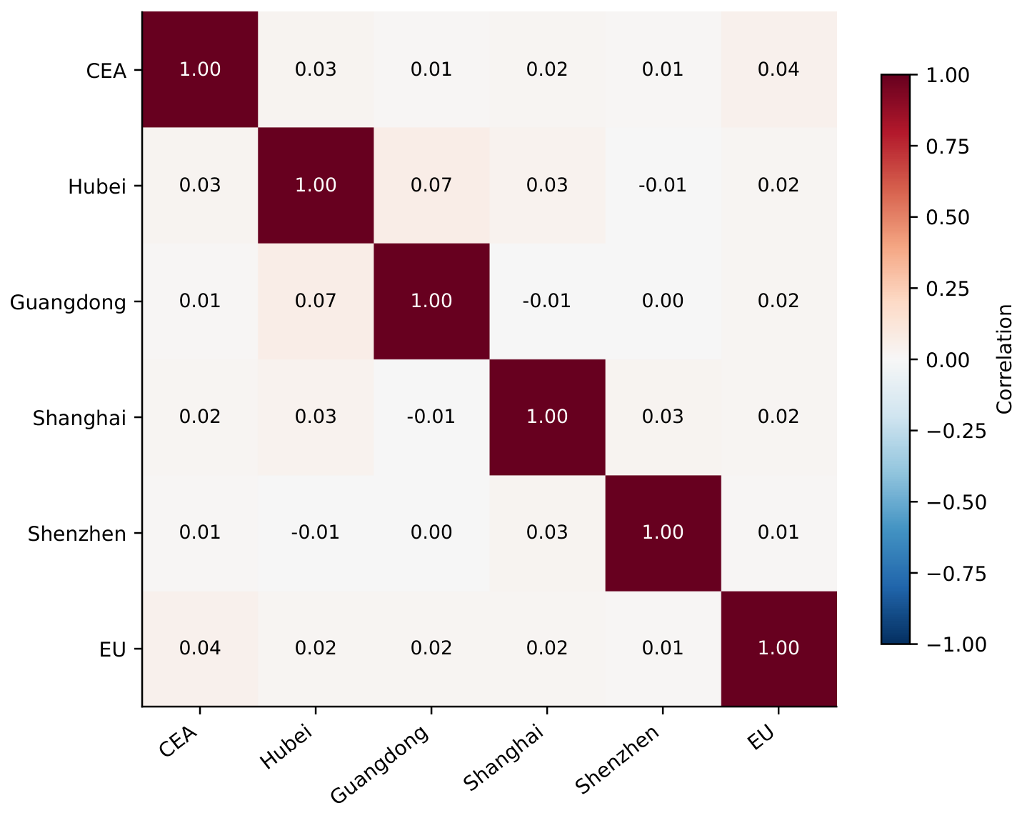
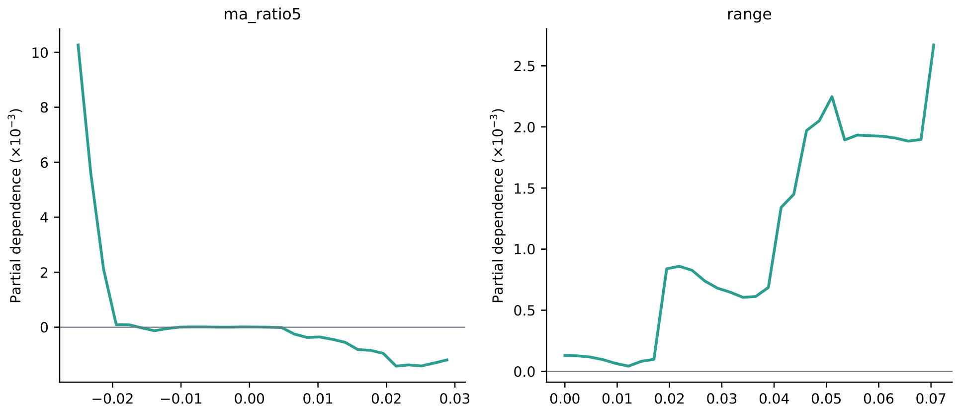
Grouped holdout permutation produces a mean MSE increase of $9.93\times {10}^{-6}$ for the technical family in the fixed-delay baseline, compared with $0.50\times {10}^{-6}$ for cross-market variables and changes near zero for the other original families. In the public augmented specification, the corresponding increases are $8.19\times {10}^{-6}$ for technical variables and $1.57\times {10}^{-6}$ for weather; the ten-day coal change is $0.02\times {10}^{-6}$, while the macro, calendar/regime and generation-proxy changes are non-positive. Figure 8 shows that contemporaneous daily CEA-return correlations with the pilot average and EU return are close to zero; correlation does not test cross-market transmission. Figure 9 and Figure 10 show a mild nonlinear fitted-model association for the five-day price gap, with larger positive gaps receiving slightly negative next-day model attributions; the wide dispersion cautions against treating this relation as a deterministic rule.

Table 9. Out-of-sample random-forest feature-family ablations. Each panel reuses its full specification’s block-specific settings; negative $\Delta$RMSE denotes lower error than that panel’s full model.

Specification	k	RMSE	MAE	Active Direction (%)	$\mathsf{\Delta }$RMSE
Panel A: original fixed-delay/final-history baseline
Full baseline	26	1.289	0.808	47.4	0.0000
Technical only	15	1.254	0.781	51.0	$-0.0348$
Without technical	11	1.379	0.875	47.6	0.0902
Without cross-market	22	1.262	0.789	47.6	$-0.0273$
Without macro	22	1.288	0.804	49.7	$-0.0008$
Without calendar/regime	23	1.289	0.808	46.8	0.0003
Panel B: public energy/weather sensitivity with exact-release macro values
Full public augmentation	31	1.275	0.801	45.7	0.0000
Technical only	15	1.253	0.781	51.0	$-0.0214$
Without technical	16	1.290	0.814	47.6	0.0150
Without weather	28	1.267	0.796	47.4	$-0.0071$
Without NBS ten-day coal	30	1.274	0.799	46.0	$-0.0008$
Without generation proxy	30	1.275	0.803	46.7	0.0008
Original 26, exact-release macro	26	1.268	0.795	46.8	$-0.0066$

separates the original baseline from the new public-data sensitivity. In Panel A, the technical-only baseline has RMSE 1.254 versus 1.289 for the full forest, while removing technical features raises RMSE to 1.379. In Panel B, the public 31-variable specification has RMSE 1.275; its technical-only counterpart reaches 1.253, whereas removing technical features raises RMSE to 1.290. Removing weather lowers RMSE to 1.267, and removing the ten-day coal measure changes it only to 1.274; removing the generation proxy changes it to 1.275. Thus, the added measures do not improve common-sample point forecasts, while the technical ordering survives the tested augmentation. The independently nested restricted specification using the one-session-lagged daily wind coal alternative has RMSE 1.274 under the 21-day generation rule and 1.280 under 28 days. Every specification remains above the random-walk RMSE of 1.242. Figure 11 presents the baseline variance-ratio and ablation evidence. H2 is supported as a conditional ordering under both tested information sets, without contradicting H1₀; it is not a claim about unavailable observed national daily load or economic causation.

5.5. Volatility

Table 10. GARCH(1,1)-t estimates and unit-persistence test.

Parameter	Estimate	p-Value
$\mu$ (mean)	$-0.020$	0.172
$\omega$ (constant)	0.061	0.223
$\alpha$ (ARCH)	0.297	<0.001
$\beta$ (GARCH)	0.703	<0.001
$\nu$ (degrees of freedom)	3.00	<0.001
Persistence $\alpha +\beta$	1.000	—
Wald test $H_0:\alpha +\beta =1$	0.000 (z)	1.000

reports the GARCH(1,1)-t estimates, $\alpha =0.297$ and $\beta =0.703$, together with the persistence diagnostic. Their sum equals 1.000, and the reported Wald diagnostic cannot distinguish it from the unit-persistence boundary ($p=1.000$). Boundary inference is non-standard, so the result does not establish exact IGARCH behavior; it does show that the fitted stationary GARCH does not identify a finite volatility half-life. The Student’s t degrees of freedom are about three, confirming heavy tails.

Table 11. Full-sample Student’s t volatility-specification comparison.

Model	Log Likelihood	AIC	BIC
EGARCH(1,1)-t	$-1923.87$	3857.73	3883.19
Asymmetric EGARCH(1,1)-t	$-1923.45$	3858.90	3889.45
GARCH(1,1)-t	$-1954.10$	3918.20	3943.66
IGARCH(1,1)-t	$-1955.81$	3919.61	3939.98
GJR-GARCH(1,1)-t	$-1954.07$	3920.13	3950.68
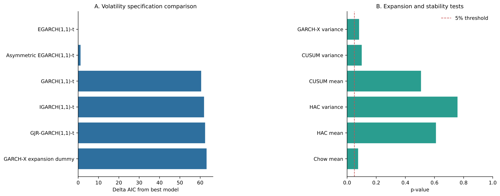
GARCH-X expansion dummy	$-1954.43$	3920.86	3951.41

reports full-sample fit. Symmetric EGARCH-t has the lowest AIC (3857.7), followed closely by asymmetric EGARCH (3858.9), approximately 59–62 points below the GARCH, IGARCH and GJR-GARCH fits.

Table 12. One-step-ahead volatility comparison on 702 common forecast dates. Absolute and squared returns are noisy proxies for latent volatility and variance.

Model	Volatility RMSE	Variance RMSE	QLIKE	Refit Failures
IGARCH-t	1.416	8.148	1.833	0
GJR-GARCH-t	1.405	8.104	1.975	1
GARCH-t	1.413	8.179	1.983	0
Asymmetric EGARCH-t	4.826	55.054	3.049	0
EGARCH-t	4.831	54.556	3.057	0

gives the common-sample one-step comparison. IGARCH has the lowest QLIKE (1.833), whereas GJR-GARCH has the lowest volatility RMSE (1.405 percentage points); GARCH is close on RMSE (1.413). The two EGARCH variants have substantially larger one-step losses despite their lower in-sample AIC. One GJR refit reports a convergence flag, which is retained rather than silently discarded. Thus, in-sample fit and out-of-sample proxy losses do not select the same model. H3a is supported only in the bounded sense of high estimated persistence; risk analysis should retain specification uncertainty rather than assign a precise shock duration.

5.6. The 2025 Expansion: Level, Volatility and Predictability

Table 13. Descriptive pre/post comparison and fixed-date break test.

Period	n	Mean Price (CNY/t)	Mean |Return| (%)	Ann. Volatility (%)
Pre-expansion	893	69.35	1.01	27.98
Post-expansion	310	72.80	1.11	29.40
Chow test on the return AR(1): F $=2.59$, $p=0.076$.

reports 893 pre-expansion and 310 post-expansion daily price observations. Average CEA prices are 69.35 CNY/t before and 72.80 CNY/t after the expansion date, while annualized unconditional volatility changes from 27.98% to 29.40%. These descriptive differences do not identify a policy parameter. The Chow test is not significant at 5% ($p=0.076$); the HAC post-expansion dummy is insignificant in the conditional mean ($p=0.610$) and squared-return variance proxy ($p=0.758$); CUSUM does not reject mean stability ($p=0.508$) or variance-proxy stability ($p=0.101$); and the GARCH-X variance dummy is also above 5% ($p=0.082$).

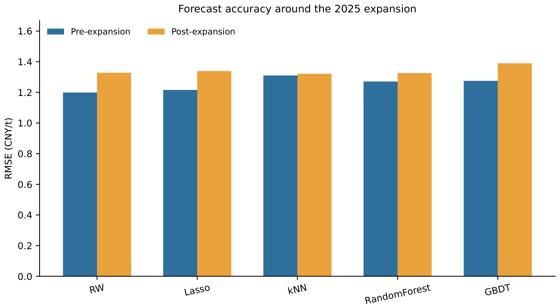
Figure 12 displays the period-specific forecasting RMSEs discussed below.

Table 14. Rolling, scanned and BIC-selected structural-instability diagnostics.

Diagnostic	Result	Expansion-Period Interpretation
HAC candidate-date scan	Minimum raw p: mean 0.151; variance proxy 0.146; all Holm $p=1.000$	No candidate date survives multiplicity correction
Return AR(1) BIC segmentation	0 breaks; BIC $=-9674.09$	No selected conditional-mean break
Log-squared-return BIC segmentation	3 breaks; 18 Apr 2022, 21 Jul 2023, 18 Oct 2024; BIC $=3261.69$	Selected volatility-proxy dates precede 26 Mar 2025
252-day rolling estimates	AR(1) $[-0.504,0.363]$; annualized volatility $[14.45,34.05]\%$	25 Mar 2025: AR(1) $=-0.140$; volatility $=23.29\%$

and Figure 13 relax dependence on a single date. Across 70 trimmed candidate dates, the smallest unadjusted HAC p-values are 0.151 for the conditional mean and 0.146 for the variance proxy, and every Holm-adjusted value equals 1.000. BIC segmentation selects no break in the return AR(1). For log squared returns, it selects three level shifts—18 April 2022, 21 July 2023 and 18 October 2024—rather than a date around 26 March 2025. The 252-day rolling AR(1) coefficient ranges from $-0.504$ to 0.363 and annualized realized volatility from 14.45% to 34.05%; immediately before the expansion date they are $-0.140$ and 23.29%, with no abrupt discontinuity visible in the rolling path. These exploratory diagnostics indicate time variation but do not associate it uniquely with the expansion.

Table 15. Out-of-sample predictability before and after the 2025 expansion.

Period	Model	n	RMSE (CNY/t)	Dir. Acc. Active (%)
Pre-expansion	Random walk	642	1.199	—
Pre-expansion	Lasso	642	1.216	51.3
Pre-expansion	k-nearest neighbors	642	1.310	51.5
Pre-expansion	Random forest	642	1.271	49.1
Pre-expansion	Gradient boosting	642	1.275	47.1
Post-expansion	Random walk	310	1.328	—
Post-expansion	Lasso	310	1.339	39.4
Post-expansion	k-nearest neighbors	310	1.321	56.1
Post-expansion	Random forest	310	1.326	44.6
Post-expansion	Gradient boosting	310	1.390	40.8
Active-direction sample: 493 pre-expansion and 289 post-expansion observations.

shows that the random walk has the lowest pre-expansion RMSE. Post-expansion, k-NN and random forest have numerical RMSEs of 1.321 and 1.326 CNY/t versus 1.328 for the random walk; the differences are small and no separate sub-period forecast-comparison test is used. The post-expansion directional accuracy of k-NN is based on 289 non-zero-return cases within 310 forecasts. Figure 14 summarizes the in-sample volatility AIC and fixed-date tests. H3b is not supported at the pre-specified 5% level, and the endogenous diagnostics do not locate a return-process break near that date.

5.7. Robustness

Table 16. Random-forest sensitivity to macro publication timing and value vintage.

Availability Schedule	RMSE	MAE	Active Direction (%)	Macro Permutation $\mathsf{\Delta }$MSE ($\times {\mathbf{10}}^{-\mathbf{6}}$)
15-day delay, final history	1.289	0.808	47.4	0.159
Exact release, final history	1.265	0.794	46.0	$-0.470$
15-day delay, first public	1.286	0.808	47.7	0.071
Exact release, first public	1.266	0.793	46.2	$-0.716$
Macro omitted	1.288	0.804	49.7	—

separates publication timing from the value vintage in a $2\times 2$ design. The fixed-delay/final-history comparator has RMSE 1.289 CNY/t. Replacing the uniform delay with the actual official release time lowers RMSE to 1.265 with final-history values and to 1.266 with first-public values. Replacing final-history values with first-public values has a much smaller effect at either timing rule: RMSE changes from 1.289 to 1.286 under the fixed delay and from 1.265 to 1.266 under exact release timing. The macro-omitted specification has RMSE 1.288. All five values remain above the random-walk RMSE of 1.242. Across the 952 common origins, exact timing changes 572 of 3808 macro cells under final-history values, whereas the joint exact-time/first-public specification differs from the fixed-delay/final-history comparator in 2254 cells. The macro family’s holdout permutation change remains small and changes sign across specifications. Thus, actual publication timing matters more for random-forest error than the first-public/final-history distinction, without reversing the benchmark ranking.

Table 17. Lower-frequency aggregation of one-step daily random-forest forecasts. Period means are evaluated on interior target periods; these are aggregated forecast summaries, not direct weekly or monthly models.

Aggregation	Periods	Exact First-Public RMSE	Macro-Omitted RMSE	Random-Walk RMSE	Exact vs. Omitted HAC p
Weekly	200	0.609	0.661	0.517	0.146
Monthly	47	0.382	0.392	0.293	0.389

reports the lower-frequency check. After excluding the two sample-edge calendar periods, weekly aggregation retains 200 periods (950 daily forecasts): exact-release/first-public macro inputs yield an RMSE of 0.609 CNY/t, compared with 0.661 when macro variables are omitted and 0.517 for the random walk. The paired HAC squared-loss comparison between the first two specifications has $p=0.146$. Monthly aggregation retains 47 periods (947 forecasts): the corresponding RMSEs are 0.382, 0.392 and 0.293 CNY/t, with $p=0.389$. Thus, macro inclusion produces a numerical reduction relative to macro omission at both aggregation levels, but the difference is not statistically significant and the random walk remains best.

The common daily sample contains 170 flat and 782 active targets. A new official macro release enters the pre-open information set on 85 targets; the flat-day rate is 21.2% on those targets and 17.5% otherwise (difference 3.6 percentage points; controlled HAC $p=0.294$). Flat targets account for 12.4% of the exact-release model’s total numerical squared-error reduction relative to macro omission, whereas active targets account for 87.6%. A joint macro-level flat-day diagnostic is sensitive to dependence treatment (HAC(20) $p=0.041$, HAC(40) $p=0.099$, HAC(60) $p=0.113$, and calendar-month-clustered $p=0.099$); autocorrelation-preserving univariate circular-shift p-values range from 0.160 to 0.632. These diagnostics do not show a robust flat-day artifact, but neither do they establish causal macro relevance or stable lower-frequency forecasting value.

The MLP ablation in Table 6 and the volatility tournament in Table 12 address model-instability risk from two directions. Stronger regularization and tighter convergence remove the neural-network outlier but do not create a forecast advantage. Conversely, the volatility specification with the best full-sample AIC performs poorly on common-sample one-step losses. Figure 15 places the macro-timing, MLP and volatility sensitivity results on common visual scales.

6. Discussion

6.1. What the Results Mean for a Young Carbon Market

The central finding is a distinction between statistical dependence and demonstrated forecast value. The 225 zero returns constitute 18.72% of the 1202-return sample. The sign-runs test removes those zeros and asks whether the remaining directions are randomly ordered; its non-rejection is therefore compatible with near-chance active-day forecasts. The two-day variance ratio and lag-1 return autocorrelation of $-0.121$ identify a local reversal component, while non-rejection at five and ten days indicates that it does not persist uniformly across longer horizons. Ljung–Box instead tests joint linear autocorrelation over several lags, and BDS tests the broader IID null. Lag-1 squared-return autocorrelation is 0.367 and remains positive through lag 10, showing why magnitude dependence and volatility clustering can coexist with weak directional ordering.

This separation provides an evidence-based adaptive-markets interpretation [65]. Participation, liquidity and compliance pressure may evolve, so flat-state clustering, reversal and volatility persistence can be transient or regime dependent rather than a stable signed conditional mean. The rolling estimates reinforce the time-varying description, while the nested tournament shows that the tested learners do not convert it into lower next-day price loss. The adaptive-markets hypothesis is an organizing interpretation, not a causal result: the present design cannot distinguish intermittent trading, price discreteness, compliance timing and participation changes as explanations. The evidence neither proves full weak-form efficiency nor rules out predictive content at other horizons or with genuinely new information; it establishes no robust advantage for the tested models, horizon and 26-variable set.

6.2. Where Machine Learning Does Add Value

Machine learning remains useful as a disciplined diagnostic. In both the 26-variable baseline and the public 31-variable sensitivity, holdout permutation and expanding-window ablation assign the largest model-output contribution to own-price technical variables. The added weather block receives smaller positive holdout attribution, yet removing it lowers expanding-window RMSE; the ten-day coal and lagged-generation contributions are negligible or unstable. Because the interpretation model never sees the final quarter during training, this is stronger than an in-sample ranking. Because the technical-only forest still fails to beat the random walk, it remains evidence about model association, not an exploitable signal or economic causation. Likewise, repeating a monthly release across eligible trading days represents a slow-moving information state, not high-frequency macro measurement; the weekly/monthly aggregation and flat-day diagnostics do not establish causal macro relevance or a stable multi-horizon gain. The result is conditional on the measured additions and does not generalize to unavailable observed national daily load or a fully timestamped daily fuel-cost panel. The MLP ablation adds a complementary lesson: optimization and regularization choices can remove an extreme error result without creating benchmark superiority, so failure diagnosis and forecast comparison are separate tasks.

6.3. Implications for Sustainable Power-Sector Management

For covered power and industrial entities, three practices follow. First, allowance procurement should not be concentrated around a single daily trough forecast, because the tested forecasts do not improve on the benchmark. Second, risk limits and stress tests should accommodate heavy tails and model uncertainty: the information-criterion and one-step volatility rankings need not select the same specification. Third, investment appraisal for low-carbon retrofits should evaluate a range of CEA paths. We do not attach a precise “weeks rather than days” duration to shocks because persistence is estimated at the unit boundary and a finite half-life is not identified.

6.4. Implications for ETS Design and Market Maturation

The fixed-date tests do not identify a statistically significant conditional-mean or variance break at the expansion date. Several explanations remain possible, including anticipation, contemporaneous demand or allocation developments and the short post-period, but the design cannot distinguish among them. The rolling and multiple-break diagnostics describe whether instability develops gradually or at other dates; they are not estimates of the expansion’s causal effect. As post-expansion observations accumulate, future work can test whether measured participation and liquidity co-evolve with dependence, volatility and forecastability.

6.5. Institutional Barriers to Daily Cross-Market Co-Movement

Figure 8’s near-zero contemporaneous correlations should be read against the institutional comparison in

Table 18. Institutional comparison relevant to cross-market price comparability.

System	Product and Compliance Boundary	Allocation and Participation	Implication for Daily Comparison
National CEA	National allowance and registry; nationally covered key emitters no longer participate in the relevant local pilot	Predominantly free, output/benchmark-linked allocation in the study period; key emitters and eligible institutions/individuals	Separate national product prevents assuming direct pilot or EU arbitrage parity
Hubei, Guangdong, Shanghai and Shenzhen pilots	Each defines local allowances, accounts and surrender eligibility under its own rules	Allocation and participant-access provisions differ across pilots and over time	Local scarcity, compliance calendars and liquidity need not map one-for-one into national CEA returns
EU ETS	EU allowance in the Union Registry under a declining cap; no EU–China allowance link located in the cited official sources	Auctioning is the default, with harmonized free allocation for eligible sectors; covered operators and eligible market participants trade under the EU market-integrity framework	Common news may co-move prices, but direct unit interchangeability and identical market depth cannot be assumed

. The national CEA, four pilots and EU ETS are separate compliance systems with different products, registries, allocation rules and eligible participants [66,67,68,69,70,71,72,73,74]. Article 13 of the national rules provides that a key emitting entity covered by the national market no longer participates in the relevant local pilot. The cited Commission material identifies the EU–Switzerland linking agreement and EU–China carbon-market cooperation; no EU–China allowance-linking agreement was located in the official sources searched [75]. Direct cross-system allowance interchangeability should therefore not be assumed. This separation limits direct arbitrage parity but does not preclude shared energy, macroeconomic or policy news, lead–lag relations at other horizons or nonlinear dependence. Near-zero daily correlation is descriptive evidence about this sample, not proof that institutions caused weak co-movement.

6.6. Comparison with Daily National-Market Studies

The findings differ from hybrid studies that report large forecasting gains [8,9] in three design choices: the target is the young national CEA price after 2021; every learner faces the same expanding information set and nested tuning; and performance is judged against a random walk with multiplicity-aware tests. They also differ from the allowance-cap framework of Wang et al. [10], which predicts an aggregate regulatory quantity rather than a next-day traded price. The relatively high model attribution to own-price history and limited daily contribution of broad external variables accord with Liao et al. [20], but the benchmark-based out-of-sample design here shows that relative attribution does not imply incremental forecast value. Relative to EU evidence on candidate energy and macroeconomic predictors [6,7], the weak daily cross-market and macro content suggests that relevance is market- and frequency-specific. Relative to structural-instability studies [4,5], the short post-expansion sample motivates the added rolling and multiple-break diagnostics rather than a policy-effect claim.

6.7. Comparison with High- and Mixed-Frequency Pilot Forecasting

Frequency labels require care. Han et al. [76] forecast weekly Shenzhen prices with daily energy, weather and environmental inputs; “high frequency” is relative to the weekly target. Wu et al. [77] forecast the daily Hubei close from daily OHLC, volume and turnover despite the term “ultra-short-term”. Duan et al. [78] and He et al. [79] use daily OHLC or range summaries for next-day Guangdong/Hubei prediction, while Chai et al. [80] decompose daily pilot prices into statistical frequency components. These designs exploit richer within-day summaries, mixed-frequency inputs or multiscale structure, but none of the cited targets is a timestamped tick or one-/five-minute order-book price.

The present daily national-market result is consequently not a contradiction of the cited pilot studies. The difference is frequency- and design-specific: those studies often use longer local histories, daily range information, decomposition and model-to-model benchmarks, whereas this study evaluates the national CEA close under a strict expanding-window random-walk comparison. Their reported gains motivate future work with archived national minute quotes, but the cited studies do not establish a tick- or minute-level forecast target and do not imply that daily predictors must beat the no-change benchmark in the younger national market.

6.8. Methodological Contribution and Robustness

The methodological contribution is an auditable sequence: impose source-specific release availability; separate exact publication timing from first-public versus final-history macro values; admit archived forecast weather rather than realized weather; preserve the published scope and uncertainty of lower-frequency energy proxies; fit preprocessing within training folds; tune inside an expanding inner window; compare models in a common expanding outer window; diagnose neural-network convergence; correct forecast tests for small samples and multiplicity; separate holdout attribution from out-of-sample prediction; and compare fixed-date, rolling, multiple-break and one-step volatility specifications before interpreting policy relevance. Figure 1, the reported model settings and Appendix A and Appendix B document the sequence.

6.9. Limitations and Future Work

Six limitations bound the claims. First, the energy sensitivity does not contain continuous official national daily observed load. Its NBS coal measure is a ten-day circulation-market price, the daily wind alternative lacks historical publication timestamps and the CarbonMonitor-Power variable is a constructed generation proxy under assumed 21-/28-day availability lags. The feature-family ordering is therefore conditional on these measured additions, although the GFS weather fields are archived pre-open forecasts. Second, the official macro panel reconstructs the first-public rate and actual release time but not every later revision state; PBOC labels current-period figures as preliminary. Third, daily OHLC aggregation cannot identify bid–ask spread, order-book depth, price impact, slippage or short announcement responses. A market-calibrated trading study consequently requires a lawfully accessible historical quote archive and a dated numerical fee schedule; this article does not infer those quantities from daily ranges. Fourth, proprietary wind row-level series are not distributed; readers without access cannot reproduce that part of the panel exactly, although Appendix A and Appendix B supply aggregate diagnostics. Fifth, only 310 post-expansion price observations are available versus 893 before expansion. Rolling and BIC segmentation reduce dependence on one date but remain exploratory, and their selected dates do not identify causes. Sixth, daily volatility is latent. Absolute and squared returns are noisy proxies, so the one-step volatility-loss ranking should be interpreted jointly with information criteria and not as a definitive model-selection result.

7. Conclusions

China’s daily national CEA returns exhibit statistically detectable dependence, although the diagnostics concern different null hypotheses and horizons: Ljung–Box and BDS reject their respective nulls, the sign-runs test does not reject sign independence, and the variance-ratio null is rejected only at the two-day horizon. The 18.72% flat-return share and positive squared-return dependence help reconcile magnitude clustering with near-random ordering of non-zero signs. Across 952 nested expanding-window forecasts, no tested model reduces price RMSE below the 1.242 CNY/t no-change benchmark. Stabilizing the MLP lowers its RMSE from 3.848 to 1.251 and removes clipped forecasts, but does not create a benchmark advantage. Exact macro release timing materially lowers the random-forest error relative to the fixed-delay comparator, whereas replacing final-history values with first-public values has a much smaller effect; neither specification beats the benchmark. The public energy/weather augmentation also remains worse than the benchmark. Technical variables retain the largest conditional attribution, and the technical-only forest reaches 1.253 CNY/t, but the ordering is not generalized to observed national daily load or a fully timestamped daily fuel-cost panel.

Volatility is heavy-tailed and estimated at the unit-persistence boundary. Symmetric EGARCH has the lowest full-sample AIC, whereas IGARCH minimizes one-step QLIKE and GJR-GARCH minimizes volatility RMSE, so model uncertainty remains material. Fixed-date and multiplicity-adjusted scans do not identify a mean or variance-proxy break around 26 March 2025. BIC segmentation selects no return-process break and places volatility-proxy shifts at earlier dates; these results do not estimate a policy effect.

The conclusion is therefore conditional: statistical structure exists, but the tested daily information sets do not deliver a stable point-forecast advantage. For sustainable power-sector management, machine learning is most credible as a transparent signal-screening and risk-diagnostic tool, while procurement and investment decisions should use broad price and volatility stress tests. Execution performance is not inferred from daily OHLC data. Future work requires timestamped national-market quotes, dated numerical fees, continuous observed national daily load and a point-in-time daily fuel-cost series, and should re-evaluate alternative horizons as the post-expansion record deepens.

References

1. Zhang, W.; Xi, B. The effect of carbon emission trading on enterprises’ sustainable development performance: A quasi-natural experiment based on carbon emission trading pilot in China. Energy Policy 2024, 185, 113960. [Google Scholar] [CrossRef] [Scilit]
2. Ministry of Ecology and Environment of the People’s Republic of China. Work Plan for Extending the National Carbon Emissions Trading Market to the Steel, Cement and Aluminium Smelting Industries. 2025. Available online: https://www.mee.gov.cn/xxgk2018/xxgk/xxgk03/202503/t20250326_1104736.html (accessed on 21 July 2026).
3. Ministry of Ecology and Environment of the People’s Republic of China. China’s National Carbon Markets Operated Smoothly and Orderly in 2025. 2026. Available online: https://www.mee.gov.cn/ywgz/ydqhbh/wsqtkz/202601/t20260101_1139528.shtml (accessed on 21 July 2026).
4. Alberola, E.; Chevallier, J.; Chèze, B. Price drivers and structural breaks in European carbon prices 2005–2007. Energy Policy 2008, 36, 787–797. [Google Scholar] [CrossRef] [Scilit]
5. Conrad, C.; Rittler, D.; Rotfuß, W. Modeling and explaining the dynamics of European Union Allowance prices at high-frequency. Energy Econ. 2012, 34, 316–326. [Google Scholar] [CrossRef] [Scilit]
6. Chevallier, J. Carbon futures and macroeconomic risk factors: A view from the EU ETS. Energy Econ. 2009, 31, 614–625. [Google Scholar] [CrossRef] [Scilit]
7. Adekoya, O.B. Predicting carbon allowance prices with energy prices: A new approach. J. Clean. Prod. 2021, 282, 124519. [Google Scholar] [CrossRef] [Scilit]
8. Zhu, B.; Wei, Y. Carbon price forecasting with a novel hybrid ARIMA and least squares support vector machines methodology. Omega 2013, 41, 517–524. [Google Scholar] [CrossRef] [Scilit]
9. Wang, N.; Guo, Z.; Shang, D.; Li, K. Carbon trading price forecasting in digitalization social change era using an explainable machine learning approach: The case of China as emerging country evidence. Technol. Forecast. Soc. Change 2024, 200, 123178. [Google Scholar] [CrossRef] [Scilit]
10. Wang, X.; Hu, W.; Bai, L.; Chang, W.; Yu, X. Forecasting the total carbon allowance cap under emission-reduction targets using a hybrid path analysis and supervised machine learning framework. Front. Environ. Sci. 2026, 14, 1757914. [Google Scholar] [CrossRef] [Scilit]
11. Tashman, L.J. Out-of-sample tests of forecasting accuracy: An analysis and review. Int. J. Forecast. 2000, 16, 437–450. [Google Scholar] [CrossRef] [Scilit]
12. Bergmeir, C.; Benítez, J.M. On the use of cross-validation for time series predictor evaluation. Inf. Sci. 2012, 191, 192–213. [Google Scholar] [CrossRef] [Scilit]
13. Diebold, F.X.; Mariano, R.S. Comparing Predictive Accuracy. J. Bus. Econ. Stat. 1995, 13, 253–263. [Google Scholar] [CrossRef] [Scilit]
14. Makridakis, S.; Spiliotis, E.; Assimakopoulos, V. Statistical and Machine Learning forecasting methods: Concerns and ways forward. PLoS ONE 2018, 13, e0194889. [Google Scholar] [CrossRef] [Scilit]
15. Goulder, L.H.; Long, X.; Lu, J.; Morgenstern, R.D. China’s unconventional nationwide CO2 emissions trading system: Cost-effectiveness and distributional impacts. J. Environ. Econ. Manag. 2022, 111, 102561. [Google Scholar] [CrossRef] [Scilit]
16. Fan, J.H.; Todorova, N. Dynamics of China’s carbon prices in the pilot trading phase. Appl. Energy 2017, 208, 1452–1467. [Google Scholar] [CrossRef] [Scilit]
17. Chang, K.; Ge, F.; Zhang, C.; Wang, W. The dynamic linkage effect between energy and emissions allowances price for regional emissions trading scheme pilots in China. Renew. Sustain. Energy Rev. 2018, 98, 415–425. [Google Scholar] [CrossRef] [Scilit]
18. Wen, F.; Zhao, H.; Zhao, L.; Yin, H. What drive carbon price dynamics in China? Int. Rev. Financ. Anal. 2022, 79, 101999. [Google Scholar] [CrossRef] [Scilit]
19. Lin, B.; Jia, Z. What are the main factors affecting carbon price in Emission Trading Scheme? A case study in China. Sci. Total Environ. 2019, 654, 525–534. [Google Scholar] [CrossRef] [Scilit]
20. Liao, M.; Long, F.; Tian, X.; Bi, F.; Tian, W.; Li, X.; Ge, C. A study on factors influencing the national carbon emission trading price in China. PLoS ONE 2025, 20, e0333788. [Google Scholar] [CrossRef] [Scilit]
21. Du, M.; Antunes, J.; Wanke, P.; Chen, Z. Ecological efficiency assessment under the construction of low-carbon city: A perspective of green technology innovation. J. Environ. Plan. Manag. 2022, 65, 1727–1752. [Google Scholar] [CrossRef] [Scilit]
22. Shao, S.; Cheng, S.; Jia, R. Can low carbon policies achieve collaborative governance of air pollution? Evidence from China’s carbon emissions trading scheme pilot policy. Environ. Impact Assess. Rev. 2023, 103, 107286. [Google Scholar] [CrossRef] [Scilit]
23. Zhu, R.; Wei, Y.; Tan, L. Low-carbon technology adoption and diffusion with heterogeneity in the emissions trading scheme. Appl. Energy 2024, 369, 123537. [Google Scholar] [CrossRef] [Scilit]
24. Hoerl, A.E.; Kennard, R.W. Ridge Regression: Biased Estimation for Nonorthogonal Problems. Technometrics 1970, 12, 55–67. [Google Scholar] [CrossRef]
25. Tibshirani, R. Regression Shrinkage and Selection Via the Lasso. J. R. Stat. Soc. Ser. Stat. Methodol. 1996, 58, 267–288. [Google Scholar] [CrossRef] [Scilit]
26. Zou, H.; Hastie, T. Regularization and Variable Selection Via the Elastic Net. J. R. Stat. Soc. Ser. Stat. Methodol. 2005, 67, 301–320. [Google Scholar] [CrossRef] [Scilit]
27. Cortes, C.; Vapnik, V. Support-vector networks. Mach. Learn. 1995, 20, 273–297. [Google Scholar] [CrossRef] [Scilit]
28. Cover, T.; Hart, P. Nearest neighbor pattern classification. IEEE Trans. Inf. Theory 1967, 13, 21–27. [Google Scholar] [CrossRef] [Scilit]
29. Breiman, L. Random Forests. Mach. Learn. 2001, 45, 5–32. [Google Scholar] [CrossRef] [Scilit]
30. Friedman, J.H. Greedy function approximation: A gradient boosting machine. Ann. Stat. 2001, 29, 1189–1232. [Google Scholar] [CrossRef] [Scilit]
31. LeCun, Y.; Bengio, Y.; Hinton, G. Deep learning. Nature 2015, 521, 436–444. [Google Scholar] [CrossRef] [Scilit] [PubMed]
32. Zhang, G. Time series forecasting using a hybrid ARIMA and neural network model. Neurocomputing 2003, 50, 159–175. [Google Scholar] [CrossRef] [Scilit]
33. James, G.; Witten, D.; Hastie, T.; Tibshirani, R. An Introduction to Statistical Learning; Springer Texts in Statistics; Springer: Berlin/Heidelberg, Germany, 2013. [Google Scholar] [CrossRef] [Scilit]
34. Hastie, T.; Tibshirani, R.; Friedman, J. The Elements of Statistical Learning; Springer Series in Statistics; Springer: Berlin/Heidelberg, Germany, 2009. [Google Scholar] [CrossRef]
35. Petropoulos, F.; Apiletti, D.; Assimakopoulos, V.; Babai, M.Z.; Barrow, D.K.; Ben Taieb, S.; Bergmeir, C.; Bessa, R.J.; Bijak, J.; Boylan, J.E.; et al. Forecasting: Theory and practice. Int. J. Forecast. 2022, 38, 705–871. [Google Scholar] [CrossRef] [Scilit]
36. Diebold, F.X. Comparing Predictive Accuracy, Twenty Years Later: A Personal Perspective on the Use and Abuse of Diebold–Mariano Tests. J. Bus. Econ. Stat. 2015, 33, 1. [Google Scholar] [CrossRef] [Scilit]
37. Clark, T.E.; West, K.D. Approximately normal tests for equal predictive accuracy in nested models. J. Econom. 2007, 138, 291–311. [Google Scholar] [CrossRef] [Scilit]
38. Lundberg, S.M.; Lee, S.-I. A Unified Approach to Interpreting Model Predictions. In Advances in Neural Information Processing Systems 30; Guyon, I., Luxburg, U.V., Bengio, S., Wallach, H., Fergus, R., Vishwanathan, S., Garnett, R., Eds.; Curran Associates, Inc.: Red Hook, NY, USA, 2017; pp. 4765–4774. Available online: https://proceedings.neurips.cc/paper_files/paper/2017/hash/8a20a8621978632d76c43dfd28b67767-Abstract.html (accessed on 15 August 2026).
39. Molnar, C. Interpretable Machine Learning: A Guide for Making Black Box Models Explainable, 2nd ed.; Independently Published: Munich, Germany, 2022; Available online: https://christophm.github.io/interpretable-ml-book/ (accessed on 7 July 2026).
40. Fama, E.F. Efficient Capital Markets: A Review of Theory and Empirical Work. J. Financ. 1970, 25, 383. [Google Scholar] [CrossRef] [Scilit]
41. Fama, E.F. Efficient Capital Markets: II. J. Financ. 1991, 46, 1575–1617. [Google Scholar] [CrossRef]
42. Engle, R.F. Autoregressive Conditional Heteroscedasticity with Estimates of the Variance of United Kingdom Inflation. Econometrica 1982, 50, 987. [Google Scholar] [CrossRef] [Scilit]
43. Bollerslev, T. Generalized autoregressive conditional heteroskedasticity. J. Econom. 1986, 31, 307–327. [Google Scholar] [CrossRef] [Scilit]
44. Nelson, D.B. Conditional Heteroskedasticity in Asset Returns: A New Approach. Econometrica 1991, 59, 347. [Google Scholar] [CrossRef] [Scilit]
45. Shanghai Environment and Energy Exchange. National Carbon Market Information and Trading Data. Available online: https://www.cneeex.com/ (accessed on 21 July 2026).
46. National Bureau of Statistics of China. National Data: Monthly CPI and PPI. Available online: https://data.stats.gov.cn/easyquery.htm (accessed on 21 July 2026).
47. National Bureau of Statistics of China. Data Release Archive: Monthly CPI and PPI Releases and Ten-Day Market Prices of Important Means of Production in Circulation. Available online: https://www.stats.gov.cn/sj/zxfb/ (accessed on 15 August 2026).
48. People’s Bank of China. Financial Statistics Reports. Available online: https://www.pbc.gov.cn/en/3688247/3688978/index.html (accessed on 21 July 2026).
49. People’s Bank of China. Monthly Financial Statistics Data Reports. Available online: https://www.pbc.gov.cn/diaochatongjisi/116219/116225/index.html (accessed on 15 August 2026).
50. NOAA National Centers for Environmental Information. Global Forecast System (GFS) 0.5 Degree, NCEI DSI 6182. Available online: https://www.ncei.noaa.gov/access/metadata/landing-page/bin/iso?id=gov.noaa.ncdc%3AC00634 (accessed on 15 August 2026).
51. National Oceanic and Atmospheric Administration. NOAA Global Forecast System (GFS), Registry of Open Data on AWS. Available online: https://registry.opendata.aws/noaa-gfs-bdp-pds/ (accessed on 15 August 2026).
52. Zhu, B.; Deng, Z.; Song, X.; Zhao, W.; Huo, D.; Sun, T.; Ke, P.; Cui, D.; Lu, C.; Zhong, H.; et al. CarbonMonitor-Power near-real-time monitoring of global power generation on hourly to daily scales. Sci. Data 2023, 10, 217. [Google Scholar] [CrossRef] [Scilit]
53. Carbon Monitor. CarbonMonitor-Power: Near-Real-Time Monitoring of Global Power Generation. Available online: https://power.carbonmonitor.org/ (accessed on 14 August 2026).
54. National Energy Administration of China. National Electricity Consumption, April 2026. Available online: https://www.nea.gov.cn/20260519/fdecbf091d654d53a9db438cdc356a5c/c.html (accessed on 11 August 2026).
55. National Energy Administration of China. National Power Load Reaches a New Peak. Available online: https://www.nea.gov.cn/20260710/02dd0d866ecd4e12855f69848a350181/c.html (accessed on 11 August 2026).
56. Pedregosa, F.; Varoquaux, G.; Gramfort, A.; Michel, V.; Thirion, B.; Grisel, O.; Blondel, M.; Prettenhofer, P.; Weiss, R.; Dubourg, V.; et al. Scikit-learn: Machine learning in Python. J. Mach. Learn. Res. 2011, 12, 2825–2830. [Google Scholar]
57. Harvey, D.; Leybourne, S.; Newbold, P. Testing the equality of prediction mean squared errors. Int. J. Forecast. 1997, 13, 281–291. [Google Scholar] [CrossRef] [Scilit]
58. Lo, A.W.; MacKinlay, A.C. Stock market prices do not follow random walks: Evidence from a simple specification test. Rev. Financ. Stud. 1988, 1, 41–66. [Google Scholar] [CrossRef] [Scilit]
59. Brock, W.A.; Dechert, W.D.; Scheinkman, J.A.; LeBaron, B. A test for independence based on the correlation dimension. Econom. Rev. 1996, 15, 197–235. [Google Scholar] [CrossRef] [Scilit]
60. Bai, J.; Perron, P. Computation and analysis of multiple structural change models. J. Appl. Econom. 2003, 18, 1–22. [Google Scholar] [CrossRef] [Scilit]
61. Shanghai Environment and Energy Exchange. National Carbon Market Daily Comprehensive Price Information, 31 December 2024. 2024. Available online: https://overview.cneeex.com/c/2024-12-31/495876.shtml (accessed on 11 August 2026).
62. Shanghai Environment and Energy Exchange. Announcement on Matters Concerning National Carbon Emission Allowance Trading. 2021. Available online: https://overview.cneeex.com/c/2021-06-22/491198.shtml (accessed on 11 August 2026).
63. Shanghai Environment and Energy Exchange. National Carbon Emissions Trading Client User Manual. 2024. Available online: https://overview.cneeex.com/upload/resources/file/2024/09/29/31622.pdf (accessed on 11 August 2026).
64. National Development and Reform Commission; Ministry of Ecology and Environment. Notice on Matters Concerning Carbon Emissions Trading Fees (NDRC Price [2026] No. 667). 2026. Available online: https://zfxxgk.ndrc.gov.cn/web/iteminfo.jsp?id=20628 (accessed on 11 August 2026).
65. Lo, A.W. The Adaptive Markets Hypothesis: Market Efficiency from an Evolutionary Perspective. J. Portf. Manag. 2004, 30, 15–29. [Google Scholar] [CrossRef] [Scilit]
66. Ministry of Ecology and Environment of the People’s Republic of China. Measures for the Administration of Carbon Emissions Trading (Trial). 2021. Available online: https://www.mee.gov.cn/gzk/gz/202112/t20211213_963865.shtml (accessed on 11 August 2026).
67. Ministry of Ecology and Environment of the People’s Republic of China. Explanation of the 2023 and 2024 National Carbon Emission Allowance Total Volume and Allocation Plan for the Power Generation Sector. 2024. Available online: https://www.mee.gov.cn/ywdt/zbft/202410/t20241021_1089827.shtml (accessed on 11 August 2026).
68. Hubei Carbon Emission Exchange. Hubei Carbon Emissions Trading Rules (2024 Revision), Official Rules Index. 2024. Available online: https://www.hbets.cn/list_62.html (accessed on 11 August 2026).
69. People’s Government of Guangdong Province. Decision of the People’s Government of Guangdong Province on Amending Certain Provincial Government Regulations (Order No. 275). 2020. Available online: https://gdii.gd.gov.cn/szfgfxwj/content/post_3023329.html (accessed on 11 August 2026).
70. Shanghai Municipal People’s Government. Shanghai Carbon Emissions Trading Administrative Measures. 2025. Available online: https://www.shanghai.gov.cn/xxzfgzwj/20250401/7dab726f8b55468c87eb920c49c0be89.html (accessed on 11 August 2026).
71. Shenzhen Municipal Ecology Environment Bureau. Shenzhen Carbon Emissions Trading Administrative Measures (2024 Revision). 2024. Available online: https://meeb.sz.gov.cn/gkmlpt/content/11/11380/post_11380726.html (accessed on 11 August 2026).
72. European Commission. About the EU Emissions Trading System. Available online: https://climate.ec.europa.eu/eu-action/carbon-markets/about-eu-ets_en (accessed on 11 August 2026).
73. European Commission. Auctioning of Allowances. Available online: https://climate.ec.europa.eu/eu-action/carbon-markets/eu-emissions-trading-system-eu-ets/auctioning-allowances_en (accessed on 11 August 2026).
74. European Commission. Ensuring the Integrity of the European Carbon Market. Available online: https://climate.ec.europa.eu/eu-action/carbon-markets/eu-emissions-trading-system-eu-ets/ensuring-integrity-european-carbon-market_en (accessed on 11 August 2026).
75. European Commission. International Carbon Market. Available online: https://climate.ec.europa.eu/eu-action/carbon-markets/eu-emissions-trading-system-eu-ets/international-carbon-market_en (accessed on 11 August 2026).
76. Han, M.; Ding, L.; Zhao, X.; Kang, W. Forecasting carbon prices in the Shenzhen market, China: The role of mixed-frequency factors. Energy 2019, 171, 69–76. [Google Scholar] [CrossRef] [Scilit]
77. Wu, L.; Tai, Q.; Bian, Y.; Li, Y. Point and interval forecasting of ultra-short-term carbon price in China. Carbon Manag. 2023, 14, 2275576. [Google Scholar] [CrossRef] [Scilit]
78. Duan, C.; Chen, Y.; He, J.; Ng, K.-H. Hybrid machine learning analysis of exogenous features in China’s Guangdong carbon market price prediction. Asian Acad. Manag. J. Account. Financ. 2026, 22, 91–120. [Google Scholar] [CrossRef] [Scilit]
79. He, J.; Ng, K.-H.; Peiris, S.; Allen, D. Modelling volatility and return based on a two-stage Log-BiACARR framework and intraday information: Evidence from Guangdong and Hubei carbon emissions trading markets. Phys. Stat. Mech. Its Appl. 2026, 681, 131097. [Google Scholar] [CrossRef] [Scilit]
80. Chai, S.; Zhang, Z.; Zhang, Z. Carbon price prediction for China’s ETS pilots using variational mode decomposition and optimized extreme learning machine. Ann. Oper. Res. 2025, 345, 809–830. [Google Scholar] [CrossRef] [Scilit]
Figure 1. Five sequential stages—data assembly, availability control, feature construction, nested forecasting and forecast evaluation—feed a sixth diagnostic stage divided into signal, risk and policy branches.
Sustainability 18 08967 g001
Figure 2. The national CEA price (left axis) and the European carbon price (right axis), 2021–2026, with the March 2025 sector-expansion date marked. The Chinese price rose through 2024, peaked near 105 CNY/t and then eased.The blue line shows the national CEA price on the left axis, and the green line shows the European carbon price on the right axis.
Sustainability 18 08967 g002
Figure 3. Daily returns (top) and GARCH(1,1)-t conditional volatility (bottom). Volatility is strongly clustered; the dashed line marks the March 2025 expansion.Daily returns (upper panel, blue) and GARCH(1,1)-t conditional volatility (lower panel, red). The orange dashed vertical line marks the March 2025 expansion.
Sustainability 18 08967 g003
Figure 4. No model beats the random walk on out-of-sample RMSE (A), and active-day directional accuracy is near the 50% chance level (B). Red dashed vertical lines represent the 50% chance level.
Sustainability 18 08967 g004
Figure 5. Out-of-sample one-step-ahead forecasts for the last 180 trading days: the random-walk and lasso forecasts essentially reproduce the previous close.
Sustainability 18 08967 g005
Figure 6. Holdout SHAP magnitudes: the price’s own short-term technical features receive the largest model-output attributions for next-day returns. The magnitudes are fitted-model associations, not causal or out-of-sample stability estimates.
Sustainability 18 08967 g006
Figure 7. SHAP summary (beeswarm) for next-day returns, showing the direction and dispersion of each feature’s model-output attribution.
Sustainability 18 08967 g007
Figure 8. Daily -return correlations are near zero between the national market, the regional pilots and the European price, indicating weak cross-market co-movement at daily frequency.
Sustainability 18 08967 g008
Figure 9. Partial -dependence profiles within the fitted forest for the two leading features, showing nonlinear model associations consistent with short-horizon mean reversion.
Sustainability 18 08967 g009
Figure 10. SHAP dependence for the five-day moving-average gap: the fitted forest maps large positive gaps to slightly negative model-predicted next-day returns.
Sustainability 18 08967 g010
Figure 11. The variance ratio is below one but significant only at the two-day horizon (A); technical-only features are the strongest random-forest family but remain above random-walk RMSE (B).
Sustainability 18 08967 g011
Figure 12. Out-of-sample price RMSE before and after the 2025 expansion date. Numerical post-period differences are small and are not treated as evidence of an abrupt expansion-period structural change.
Sustainability 18 08967 g012
Figure 13. Rolling 252-day return AR(1) and annualized realised-volatility estimates, with BIC-selected log-squared-return break dates and the pre-specified expansion date marked. The paths are descriptive and do not identify policy causation.
Sustainability 18 08967 g013
Figure 14. Symmetric EGARCH has the lowest full-sample AIC (A), while none of the fixed expansion-date or stability tests reaches the 5% threshold (B).
Sustainability 18 08967 g014
Figure 15. Selected robustness diagnostics: macro publication-timing and first-public-value sensitivity, MLP stabilization and common-sample one-step volatility loss. Lower values indicate smaller forecast loss within each panel; scales differ across panels.The dashed vertical line in Panels (a,b) marks the random-walk RMSE benchmark of 1.242 CNY/t.
Sustainability 18 08967 g015