Article

Coordinated Resilience of Urban–Cropland–Population–Industry–Ecology Systems Under Water Constraints: Evidence from Nine Provincial Regions Along the Yellow River

School of Water Conservancy and Transportation, Zhengzhou University, Zhengzhou 450001, China
*
Author to whom correspondence should be addressed.
Sustainability 2026, 18(17), 8779; https://doi.org/10.3390/su18178779
Submission received: 18 July 2026 / Revised: 15 August 2026 / Accepted: 25 August 2026 / Published: 27 August 2026

Abstract

Resource constraints in large river basins operate through interacting urban, agricultural, demographic, industrial, and ecological systems. This study develops a coordinated resilience framework for the Urban–Cropland–Population–Industry–Ecology (UCPIE) system using panel data from nine provincial-level regions along the Yellow River during 2000–2023. Coordinated and subsystem resilience were estimated with hierarchical entropy-weighted TOPSIS. Complementary disparity measures were used to assess interprovincial inequality and convergence, while relative shortage shares and indicator obstacle degrees supported structural diagnosis. Mean coordinated resilience increased from 0.2485 to 0.4107. Resilience in the Urban and Ecology subsystems increased rapidly, whereas Cropland resilience increased only marginally. The corrected Gini coefficient increased from 0.1740 in 2000 to 0.1983 in 2008 and declined to 0.1537 by 2023. The σ series indicated significant relative convergence even as absolute dispersion widened. The dominant shortage shifted from Urban and Ecology in the first stage to Population in the third stage, accompanied by a larger Cropland share. Per capita water resources and the proportion of effectively irrigated area reached obstacle degrees of 14.63% and 12.89%, respectively, in the third stage. The higher nine-region mean did not remove the provincial hierarchy, and the main internal constraints changed over time.

1. Introduction

Global water scarcity, climate change, rapid urbanization, and industrial transition are continuously reshaping resource constraints, spatial patterns, and development pathways in large river basins. Large river basins must sustain ecological functions, food production, energy supply, and regional development under increasingly tight water constraints. Climate change, urbanization, and industrial restructuring alter both water demand and its spatial distribution. These pressures are rarely confined to one sector. Weaknesses in urban services, agricultural water use, population carrying capacity, industrial structure, or ecological protection can reinforce one another. Basin sustainability depends on how these systems adjust together over time, not simply on aggregate economic growth or water-use efficiency. Assessing long-term adaptation therefore requires evidence on both overall performance and the internal constraints that limit it.
The “Four Water–Four Determinations” principle in China links urban development, land use, population scale, and industrial structure to local water availability and carrying capacity. Within this framework, ecological protection is integrated by coordinating water allocation for production, domestic needs, and ecological functions under water-resource carrying limits [1]. It provides the policy basis for examining sustainable development in the Yellow River Basin. Here, water is treated as a constraint shared by the Urban, Cropland, Population, Industry, and Ecology subsystems [2], not as a separate sixth subsystem. This framing supports an assessment of whether their combined development remains compatible with long-term water-resource limits. Recent work has also treated human–water regulation as a constrained optimization problem spanning water resources, socioeconomic development, and ecological conditions [3].
Resilience offers a useful lens for this assessment. Initially developed to describe the persistence of ecological systems under disturbance, the concept now encompasses resistance, recovery, and adaptation in social–ecological, urban, and regional systems [4,5,6,7]. Its value for basin research lies in the attention paid to adjustment under sustained external pressure and internal constraint. No single sector determines this capacity. Urban development, cropland use, population carrying capacity, industrial transition, and ecological functions contribute jointly, and uneven progress among them can leave structural bottlenecks even as aggregate performance improves.
Water resources have long been a major focus of research on the Yellow River Basin. Sun et al. [8] assessed water-resource security from the perspective of water-security system resilience and identified its main influencing factors. Other studies examined differences in water-resource system resilience across provinces and showed that water availability, water-use efficiency, and ecological constraints play important roles in long-term basin adaptation [9,10,11]. Research has also extended to urban, cropland, and ecological systems. Ji et al. [12] investigated the spatiotemporal changes and drivers of urban resilience, while later studies explored its links with cropland-use efficiency and urban ecological resilience [13,14]. Urban ecological resilience also shows clear spatial and temporal differences across the basin [15,16]. Huang et al. [17] found similar patterns in ecological resilience and reported that both natural and socioeconomic conditions affect its evolution. Beyond individual systems, studies of the water–energy–food nexus, water resource–water environment–water ecology relationships, and the water–land–energy–carbon nexus have shown close links and trade-offs among water use, food production, energy development, land allocation, environmental quality, and ecological security [18,19,20,21,22,23]. Yang et al. [24] further developed an uncertainty-aware multi-objective model for the Heihe Irrigation Area that jointly considered water productivity, carbon emissions, and agricultural competitiveness. In the Hetao Irrigation District, Yang et al. [25] used a two-stage multiobjective approach to compare agricultural water–energy–food allocation options. At the basin scale, Han et al. [26] assessed competition and synergy in water use between energy and food production in the Yellow River Basin by considering both water quantity and water quality. A basin-wide assessment by Hou et al. [27] found that water–energy–food adaptation differed among the upper, middle, and lower reaches. Competition for limited water between energy and food production further highlights the importance of irrigation support and agricultural water allocation [28,29].
Overall, previous studies have revealed complex relationships among resource use, spatial carrying capacity, and ecological support in the Yellow River Basin from the perspectives of water resources, urban systems, cropland systems, ecology, and cross-sectoral linkages. These studies provide an important basis for multi-system integrated assessment. However, three aspects still require further development. First, regarding the scope of the systems considered, existing studies have mostly focused on single systems such as water resources, urban systems, cropland systems, or ecological resilience. Multi-system studies have mainly examined limited system combinations such as the water–energy–food nexus or water resource–water environment–water ecology relationships [30,31,32,33]. Urban, Cropland, Population, Industry, and Ecology (UCPIE) have not yet been sufficiently integrated into a unified resilience framework in which water resources act as a shared constraint across these subsystems, limiting the ability to characterize the multi-subsystem support structure of regional adaptive capacity in large river basins. Second, in terms of regional disparity analysis, most studies have focused on resilience-level measurement, spatial pattern identification, or influencing factor interpretation, while insufficient attention has been given to whether interprovincial disparities expand, decline, or converge during long-term evolution. Third, in terms of structural diagnosis, existing assessments often remain at the level of overall index comparison or single-system explanation [34]. Less attention has been paid to the relative shortages, structural imbalances, and stage-wise changes among the five UCPIE subsystems behind improvements in coordinated resilience, making it difficult to explain the coexistence of rising overall levels and persistent local structural bottlenecks.
This study addresses these questions using a panel of nine provincial-level regions along the Yellow River from 2000 to 2023. UCPIE coordinated resilience is defined as the combined capacity of the five subsystems to support regional adaptation under resource and environmental constraints, with water treated as a shared constraint across them. Hierarchical entropy-weighted TOPSIS is used to estimate coordinated and subsystem resilience. Trend, disparity, and σ-convergence analyses characterize temporal and regional change, while relative shortage shares and indicator obstacle degrees identify structural constraints. The analysis asks whether coordinated resilience improved, whether provincial disparities converged, and how the dominant bottlenecks changed across stages.

2. Materials and Methods

2.1. UCPIE Systems Resilience Framework and Indicator System

2.1.1. UCPIE Systems Resilience Framework

In the UCPIE framework, water resources are embedded in all five subsystems through supply security, consumption, use efficiency, recycling, and ecological maintenance. Water is modeled as a shared constraint, not a sixth subsystem. Urban, Cropland, Population, Industry, and Ecology are treated as water-dependent components of regional resource use and carrying capacity. Their combined performance is examined through temporal change, provincial disparity, and structural diagnosis.
Regional resilience describes the capacity of a regional system to withstand disturbance, adjust to change, and sustain development. In resource-constrained basins, this capacity depends on the combined performance of multiple subsystems [4,5,6,7]. The proposed UCPIE framework distinguishes five components. Urban represents infrastructure and public services; Cropland represents land use and agricultural carrying capacity; Population captures resource pressure and well-being; Industry describes structural stability and adaptive capacity; and Ecology represents environmental security and ecological support.
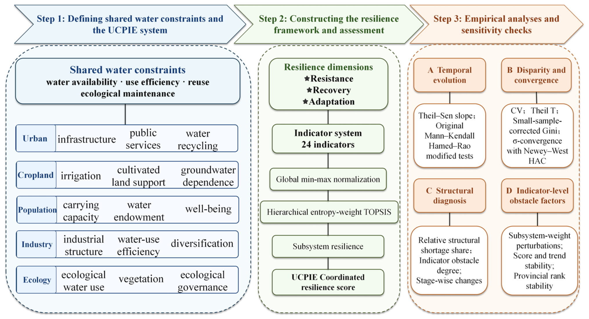
UCPIE coordinated resilience combines integrated measurement with structural diagnosis. In this study, coordination denotes the combined support provided by the five subsystems; it is not a measure of pairwise coupling or causal interaction. The coordinated resilience index summarizes their overall adaptive performance. Relative structural shortage shares and indicator obstacle degrees identify internal weaknesses and their changes across stages. Figure 1 presents the analytical framework.

2.1.2. Indicator System

This study constructs an indicator system for the UCPIE subsystems from three resilience dimensions: resistance, recovery, and adaptation. Resistance reflects the ability of a subsystem to maintain its basic structure and functions under external pressures. Recovery captures the ability of a subsystem to restore operation and obtain support after a disturbance. Adaptation represents the ability of a subsystem to respond to long-term constraints through efficiency improvement, structural adjustment, and resource allocation.
Indicators were selected for their relevance to resistance, recovery, or adaptation and their connection to water-related constraints under the “Four Water–Four Determinations” principle. We also required consistent provincial definitions and comparable observations for all nine regions throughout 2000–2023. Because long-term data availability differed among domains, the number of indicators varies by subsystem. Although the indicator counts differ, each subsystem receives a total weight of 0.20 under the hierarchical weighting scheme described in Section 2.2.2.
The content of the indicators follows the role assigned to each subsystem. Within the urban subsystem, urbanization and the built-up area ratio capture urban development and the spatial concentration of service infrastructure, while reclaimed water use, wastewater treatment, green coverage, and road density reflect the capacity of urban systems to manage growth and adjust to water-related constraints [35,36]. Irrigated agriculture depends not only on the amount of water applied, but also on effective irrigation coverage, irrigation efficiency, public support, and reliance on groundwater [29,37,38]. Population size and density describe demand pressure; per capita GDP and disposable income show the economic resources available for adjustment; and per capita water resources and domestic water use connect welfare to local water limits [36,39]. Industrial water demand and water intensity are considered alongside industrial diversity, since efficiency and structural concentration represent different sources of vulnerability [40]. Ecological water provision, vegetation condition, soil-erosion control, and greening were used to capture the water, vegetation, and land-protection functions that sustain ecological resilience [41].
The final indicator system includes 24 indicators, comprising 17 positive indicators and 7 negative indicators. For positive indicators, higher values indicate stronger support for subsystem resilience. For negative indicators, higher values indicate greater resource consumption, spatial pressure, or system exposure. The direction of each indicator remains unchanged throughout the study period. The full indicator system is presented in Table 1.

2.2. Resilience Assessment Method

2.2.1. Global Min–Max Normalization

To eliminate differences in indicator units and magnitudes, this study applied global min–max normalization to transform the raw data into dimensionless values. Unlike year-by-year normalization, this approach pools all 216 province–year samples from the nine provincial regions during 2000–2023 and determines the maximum and minimum values for each indicator from the full sample. The same set of extrema is then used for all years, thereby preserving actual interregional and intertemporal variations.
Positive and negative indicators were normalized using Equations (1) and (2), respectively:
z qj = x qj − x j , min x j , max − x j , min
z qj = x j , max − x qj x j , max − x j , min
where xqj denotes the raw value of indicator j for sample q; xj,min and xj,max denote the minimum and maximum values of indicator j among all 216 province–year samples, respectively; zqj denotes the normalized value of indicator j for sample q; q represents a province–year sample; and j represents the indicator index. After normalization, all indicators were converted into benefit-oriented indicators, for which higher values indicate better resilience performance. The normalized values theoretically range from 0 to 1.

2.2.2. Hierarchical Entropy Weighting

Because the five UCPIE subsystems contain different numbers of indicators, this study adopted a hierarchical weighting scheme. First, entropy weights were calculated independently within each subsystem, so that the indicator weights within each subsystem summed to 1. Second, equal weights were assigned to the five UCPIE subsystems when calculating coordinated resilience, with each subsystem given a weight of 0.20. This design prevents subsystems with more indicators from receiving a larger total weight in the integrated assessment simply because they contain more indicators.
The entropy-weighting method determines objective indicator weights according to the dispersion of each indicator across the full sample. The indicator proportion, information entropy, entropy normalization coefficient, information utility value, and within-subsystem entropy weight were calculated using Equations (3)–(7), respectively:
p qj = z qj ∑ q = 1 m z qj
e j = − k ∑ q = 1 m p qj ln ( p qj )
k = 1 ln ( m )
d j = 1 − e j
w js = d j ∑ h ∈ J s d h
where p qj denotes the proportion of indicator j for sample q; zqj denotes the normalized value; ej denotes the information entropy of indicator j; k denotes the entropy normalization coefficient; m denotes the number of samples, which is 216 in this study; dj denotes the information utility value of indicator j; wjs denotes the entropy weight of indicator j within subsystem s; h denotes the summation index for indicators within subsystem s; and Js denotes the set of indicators included in subsystem s.

2.2.3. TOPSIS-Based Resilience Assessment

After obtaining the within-subsystem indicator weights, this study used the technique for order preference by similarity to an ideal solution (TOPSIS) to calculate the resilience indices of the five UCPIE subsystems: Urban, Cropland, Population, Industry, and Ecology. TOPSIS evaluates each sample according to its relative distance from the positive and negative ideal solutions, thereby measuring its closeness to the ideal state within the sample set [42]. Because all indicators had been normalized as benefit-oriented indicators, the positive ideal solution was defined by the maximum value and the negative ideal solution by the minimum value.
The weighted normalized value, positive ideal solution, negative ideal solution, distances to the positive and negative ideal solutions, subsystem TOPSIS resilience index, and UCPIE coordinated resilience were calculated using Equations (8)–(14), respectively:
v qj = w js × z qj
A sj + =   max q ( v qj ) ,   j ∈ J s
A sj − = min q ( v qj ) ,   j ∈ J s
D qs + = ∑ j ∈ J s ( v qj − A sj + ) 2
D qs − = ∑ j ∈ J s ( v qj − A sj − ) 2
R qs = D qs − D qs + + D qs −
CR it = R it , Urban + R it , Cropland + R it , Population + R it , Industry + R it , Ecology 5
where vqj denotes the weighted normalized value of indicator j for sample q; A s j + and A s j − denote the positive and negative ideal values of indicator j within subsystem s, respectively; D q s + and D q s − denote the distances of sample q from the positive and negative ideal solutions within subsystem s, respectively; Rqs denotes the TOPSIS resilience index of sample q for subsystem s; and CR it denotes the UCPIE coordinated resilience of provincial region i in year t. The index obtained from Equation (14) was used as the integrated measure of UCPIE coordinated resilience.
Here, Rqs is a dimensionless relative-closeness score between 0 and 1, with larger values indicating closer proximity to the positive ideal solution. TOPSIS was applied separately within each subsystem so that every domain retained an interpretable relative-closeness score for structural diagnosis. The five subsystem scores were then combined using fixed equal weights, consistent with their treatment as coequal dimensions. Applying TOPSIS only at the final level would address a different question: the relative closeness of the five-score profile to a new set of subsystem-level ideal points. The present hierarchy therefore retains the domain-specific TOPSIS scores and uses a transparent equal-weight rule for final aggregation.

2.2.4. Subsystem-Weight Sensitivity Analysis

The five weights in Equation (14) govern the additive aggregation of parallel subsystem scores. Equal weights were retained in the baseline model because the five subsystems were treated as coequal dimensions, while entropy weights distinguished indicators within each subsystem. To examine dependence on this choice, one subsystem weight was varied at a time. The focal weight was set to 0.10 and 0.30; the other four weights were adjusted equally to 0.225 and 0.175, respectively, so that all weights remained positive and summed to 1. This produced ten alternative weighting schemes without changing the five subsystem indices. Each scheme was compared with the baseline using Spearman correlations for the 216 sample scores, the annual nine-region mean series, and the long-term provincial ranks. We also compared the annual Theil–Sen slope, the Hamed–Rao modified Mann–Kendall result, the largest 2023 rank shift, and the overlap of the top and bottom three regions.
The sensitivity analysis assesses changes in the outer subsystem weights while retaining the data-derived entropy weights within each subsystem.

2.3. Disparity and Convergence Analysis

2.3.1. Temporal Trend Estimation

To identify long-term trends in coordinated resilience and subsystem resilience, this study employed Theil–Sen slope estimation and the Hamed–Rao modified Mann–Kendall test. The Theil–Sen estimator is a nonparametric method that estimates the long-term rate of change using the median of all pairwise slopes in a time series, making it less sensitive to outliers and non-normal distributions. The Mann–Kendall test is widely used to detect monotonic trends in time-series data, while the Hamed–Rao modification further accounts for the potential influence of serial autocorrelation on significance testing [43,44,45].
For a provincial region or the nine-region average series, let Xi and Xj denote the resilience values in years i and j, respectively, and let n denote the length of the time series. The Theil–Sen slope, Mann–Kendall statistic, sign function, variance, standardized statistic, Hamed–Rao corrected variance, and corrected Z statistic were calculated using Equations (15)–(21), respectively:
β = median { X j − X i j − i } ,   1 ≤ i < j ≤ n
S = ∑ i = 1 n − 1 ∑ j = i + 1 n sign ( X j − X i )
sign ( X j − X i ) = { 1 ,   X j − X i   >   0 ;   0 ,   X j − X i = 0 ;   − 1 ,   X j − X i   <   0 }
Var ( S ) = n ( n − 1 ) ( 2 n + 5 ) − ∑ p t p ( t p − 1 ) ( 2 t p + 5 ) 18
Z = { S − 1 Var ( S ) ,   S   >   0 ;   0 ,   S =   0 ; S + 1 Var ( S ) ,   S   <   0 }
Var * ( S ) = Var ( S )   ×   CF
Z * = { S − 1 Var * ( S ) ,   S   >   0 ;   0 ,   S = 0 ; S + 1 Var * ( S ) ,   S   <   0 }
where Xi and Xj denote the resilience values in years i and j, respectively; n denotes the length of the time series; β denotes the Theil–Sen slope; S denotes the Mann–Kendall test statistic; tp denotes the number of tied values in the p group; Var ( S ) denotes the uncorrected variance; CF denotes the Hamed–Rao autocorrelation correction factor; Var * ( S ) denotes the corrected variance; and Z* denotes the corrected standardized statistic. A series was considered to have a significant increasing trend when β > 0 and the Hamed–Rao modified Mann–Kendall test was statistically significant. Conversely, a series was considered to have a significant decreasing trend when β < 0 and the test was statistically significant.
For descriptive comparison, the 2000–2023 study period was divided a priori into three equal eight-year windows: 2000–2007, 2008–2015, and 2016–2023. These windows were not derived from breakpoint detection or policy-event timing; differences among them are interpreted as variation across fixed periods rather than statistically identified structural breaks.

2.3.2. Regional Disparity Measures

Five complementary measures were used to characterize interprovincial disparity. The sample standard deviation measures the absolute spread of coordinated resilience, while the coefficient of variation scales that spread by the annual mean. The small-sample corrected Gini coefficient summarizes pairwise inequality and reduces downward bias arising from the nine-region sample [46]. The Theil T index measures distributional unevenness from an information-theoretic perspective [47]. Finally, the annual standard deviation of log-transformed resilience forms the σ series, whose decline indicates σ-convergence. Using these measures together separates changes in absolute gaps, relative dispersion, inequality, and convergence.
The annual mean, sample standard deviation, annual cross-sectional coefficient of variation, standard Gini coefficient, small-sample corrected Gini coefficient, Theil T index, and σ series were calculated using Equations (22)–(28), respectively:
mean t = 1 N   ∑ i = 1 N CR it
SD t = ∑ i = 1 N ( CR it − mean t ) 2 N − 1
CV t R = SD t mean t
G t = ∑ i = 1 N ∑ l = 1 N | CR it − CR lt | 2 N 2 mean t
G t c = N N − 1 G t
T t = 1 N   ∑ i = 1 N [ CR it mean t ln ( CR it mean t ) ]
σ t = SD [ ln ( CR 1 t ) , ln ( CR 2 t ) , … , ln ( CR Nt ) ]
where CRit denotes the UCPIE coordinated resilience of provincial region i in year t; meant denotes the mean coordinated resilience of the nine provincial regions in year t; SDt denotes the sample standard deviation in year t; CV t R denotes the annual regional cross-sectional coefficient of variation; Gt denotes the standard Gini coefficient; G t c denotes the small-sample corrected Gini coefficient; Tt denotes the Theil T index; σt denotes the σ value in year t; N denotes the number of provincial regions, which is 9 in this study; and i and l denote provincial-region indices.
Because coefficients of variation are used at different analytical dimensions in the following sections, their notation is distinguished explicitly. CVT denotes a temporal coefficient of variation calculated across years for a specified annual resilience series; it is applied to the nine-region mean, each UCPIE subsystem mean, and each provincial series to evaluate temporal stability. CVtR denotes the annual regional cross-sectional coefficient of variation among the nine provincial regions in year t [Equation (24)]. CVqS, introduced later in Equation (32), denotes the structural coefficient of variation among the five UCPIE subsystem resilience values within sample q. These three symbols therefore distinguish temporal fluctuation, interprovincial dispersion, and within-sample subsystem imbalance.

2.3.3. σ-Convergence Test

σ-convergence was used to determine whether the dispersion of coordinated resilience among the nine provincial regions declined over time. After deriving the annual σ series using Equation (28), this study estimated the linear trend of the σ series using Equation (29):
σ ^ t   =   a   +   b · t ,   ε t   =   σ t − σ ^ t
where σ ^ t denotes the fitted σ value in year t derived from the linear trend;   σ t denotes the observed σ value calculated using Equation (28); a denotes the intercept; b denotes the time trend coefficient; t denotes the time index; and εt denotes the residual, defined as the difference between the observed and fitted σ values. Significant σ-convergence was identified when b < 0 and the trend coefficient was statistically significant. Because the annual series may contain heteroskedasticity and serial correlation, the standard error of the regression was estimated using the Newey–West heteroskedasticity and autocorrelation-consistent covariance estimator, with the maximum lag set to 2 [48].

2.4. Structural Diagnosis Method

To identify internal structural bottlenecks that remained during the improvement of coordinated resilience, this study conducted structural diagnosis at both the subsystem and indicator levels. First, relative structural shortage shares were calculated based on the TOPSIS resilience indices of the five UCPIE subsystems to identify the relative weaknesses among Urban, Cropland, Population, Industry, and Ecology. Second, indicator obstacle degrees were calculated based on standardized indicator gaps and effective weights to further identify the specific indicator sources underlying subsystem-level bottlenecks.

2.4.1. Relative Structural Shortage Share Method

At the subsystem level, the relative structural shortage share was used to measure the relative weakness of each UCPIE subsystem within a given sample. The relative structural shortage share, subsystem resilience range, and subsystem coefficient of variation were calculated using Equations (30)–(32), respectively:
B qs = 1 − R qs ∑ r = 1 5 [ 1 − R qr ] × 100 %
Range q = max ( R q 1 , R q 2 , … , R q 5 ) − min ( R q 1 , R q 2 , … , R q 5 )
CV q S = SD ( R q 1 , R q 2 , … , R q 5 ) Mean ( R q 1 , R q 2 , … , R q 5 )
where Bqs denotes the relative structural shortage share of subsystem s in sample q; Rqs denotes the TOPSIS resilience index of sample q for subsystem s; r denotes the subsystem index; Rangeq denotes the range among the resilience indices of the five UCPIE subsystems in sample q; and CV q   S denotes the structural coefficient of variation among the resilience indices of the five UCPIE subsystems in sample q. The relative structural shortage share is used to identify relative weaknesses among the five UCPIE subsystems. It does not indicate an absolute decline in any subsystem. Rather, it focuses on structural balance and should not be interpreted as equivalent to the overall level of coordinated resilience.
For each subsystem, 1 − R qr is the complement of its relative-closeness score and represents a normalized deficit in closeness to the positive ideal, rather than the original Euclidean distance to that ideal. Dividing this value by the sum across the five subsystems gives each subsystem’s share of the total relative deficit within the same sample. The five shares sum to 100% and describe the composition of structural shortage; they do not form a second resilience index or measure absolute deterioration.

2.4.2. Indicator-Level Obstacle Degree

At the indicator level, the indicator obstacle degree was used to further identify the specific sources of subsystem-level structural bottlenecks. Because all indicators had been normalized so that higher values represented better resilience performance, the indicator deviation degree, effective indicator weight, indicator obstacle degree, and aggregated subsystem obstacle degree were calculated using Equations (33)–(36), respectively:
F qj = 1 − z qj
W j eff = W s   ×   w js
O qj = F qj   ×   W j eff ∑ k = 1 24 [ F qk   ×   W k eff ] ×   100 %
O qs = ∑ j ∈ J s O qj
where Fqj denotes the deviation degree of indicator j in sample q; zqj denotes the normalized value; W j eff denotes the effective weight of indicator j; Ws denotes the overall weight of subsystem s, which is 0.20 in this study; wjs denotes the entropy weight of indicator j within subsystem s; Oqj denotes the obstacle degree of indicator j in sample q; Oqs denotes the aggregated indicator obstacle degree of subsystem s in sample q; J s denotes the set of indicators included in subsystem s; and k denotes the summation index across the 24 indicators. The indicator obstacle degree is jointly determined by the standardized indicator gap and the effective weight. A higher obstacle degree indicates a stronger relative constraint within the sample, but it does not necessarily imply an absolute deterioration of the indicator. Indicator obstacle degree analysis was used to explain the specific indicator sources underlying subsystem-level bottlenecks.

2.5. Study Area and Data Sources

The Yellow River rises in the Bayan Har Mountains on the Qinghai–Tibet Plateau and flows through nine provincial regions before reaching the Bohai Sea. Its main stream extends 5464 km, and the basin covers approximately 752,400 km2. Strong upstream–downstream contrasts in elevation, climate, land use, and economic development coincide with severe water constraints. The basin contains about 2% of China’s water resources but supports nearly 12% of the national population, 17% of its cropland, and more than 50 large and medium-sized cities. Its water-resource utilization rate is about 80%. High sediment loads and fragile ecosystems add further pressure, making the basin suitable for examining the joint adaptation of the five UCPIE subsystems.
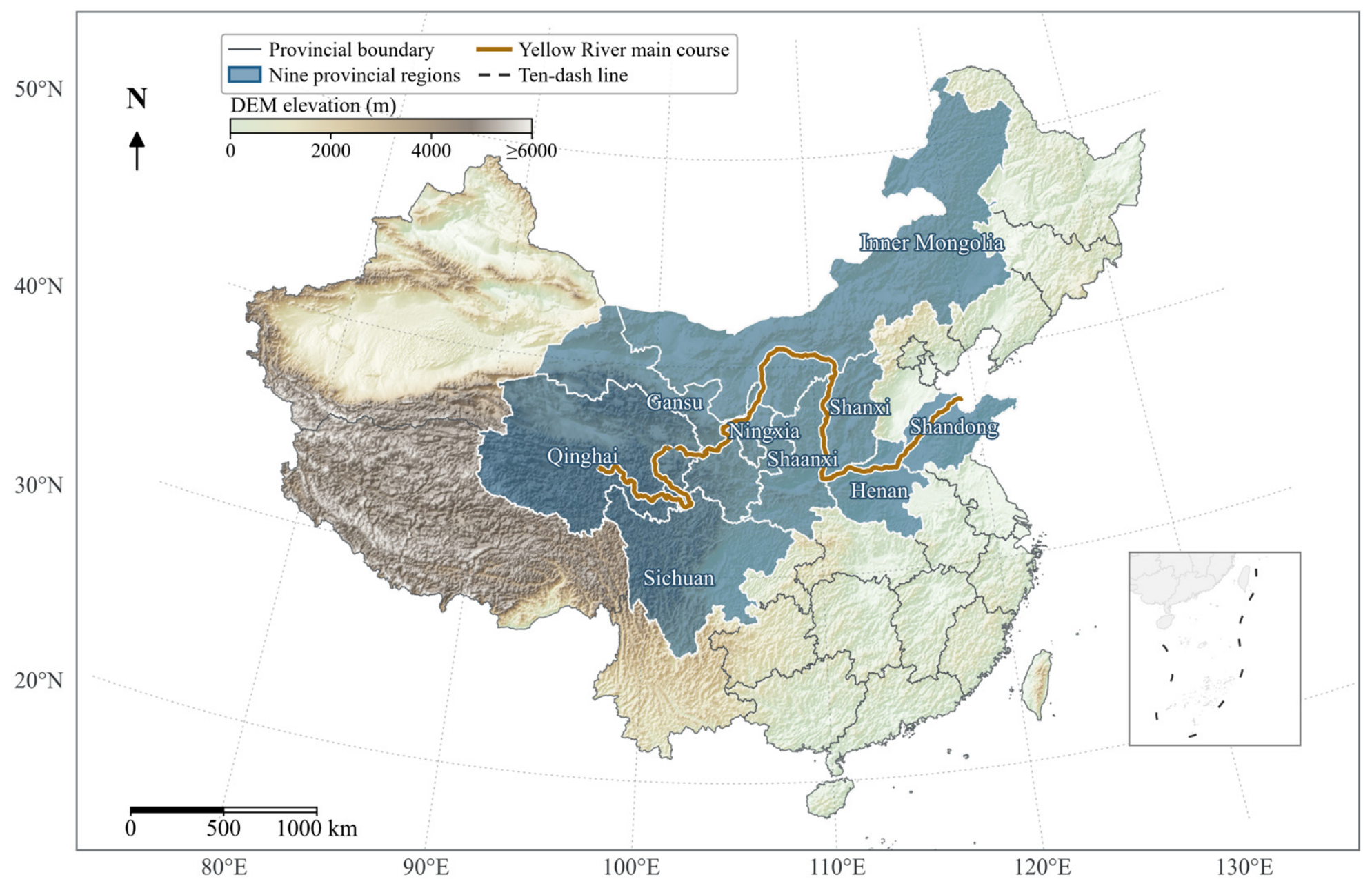
Figure 2 shows the nine provincial regions included in the analysis: Qinghai, Sichuan, Gansu, Ningxia, Inner Mongolia, Shaanxi, Shanxi, Henan, and Shandong. The unit of analysis is the complete provincial-level administrative region rather than the portion of each province located within the hydrological boundary of the Yellow River Basin; all indicators therefore refer to province-wide values. The 2000–2023 panel contains 216 province–year observations. Socioeconomic and land-use data were drawn from national and provincial statistical yearbooks and bulletins. Water-related variables came from water resources bulletins, and environmental variables from environmental statistics yearbooks and ecological environment bulletins.
Isolated internal gaps in a time series were filled by linear interpolation. When values were missing at the beginning or end of a series, we checked adjacent-year changes against the corresponding statistical yearbook or bulletin before filling the gap. Indicators with extensive unresolved gaps were excluded. We then checked units, statistical definitions, and abrupt year-to-year changes across the assembled panel. Corrections were made only when an official series or a clear transcription, decimal-place, or unit error identified the problem. Other observed fluctuations were retained. No province–year observation was removed, and the data were not smoothed or winsorized. The resulting dataset contains 216 complete province–year observations for 24 indicators, with no missing or non-finite values. Per capita GDP and per capita disposable income were recorded at current prices, following the source yearbooks.

3. Results

3.1. Temporal Evolution of Coordinated Resilience

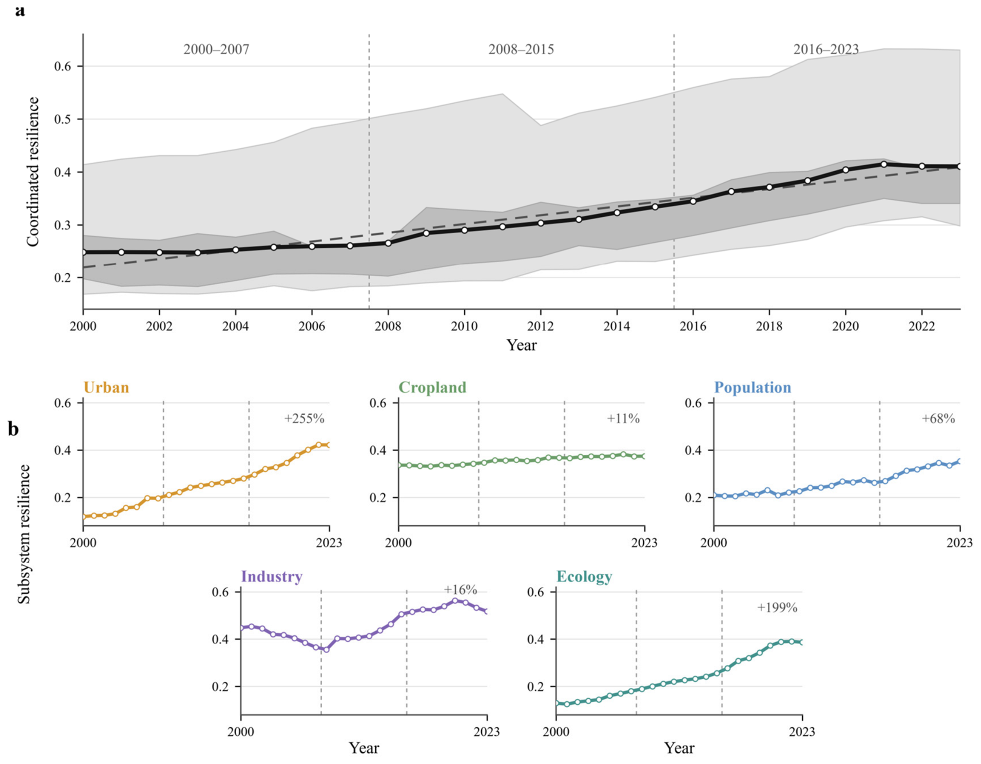
Coordinated resilience increased across all nine provincial-level regions along the Yellow River between 2000 and 2023 (Figure 3). The nine-region mean rose from 0.2485 to 0.4107, a cumulative increase of 65.28% (Table 2). The Theil–Sen slope was 0.00847 yr−1, and the Hamed–Rao modified Mann–Kendall test indicated a significant monotonic trend (p < 0.001).
Subsystem trends differed markedly. Urban resilience increased from 0.1187 to 0.4218 (+255.24%), and Ecology resilience from 0.1295 to 0.3868 (+198.60%). Population resilience rose from 0.1432 to 0.3528. Cropland resilience increased by only 11.28%, from 0.3364 to 0.3744. Industry resilience remained comparatively high and reached 0.5177, 15.53% above its 2000 value of 0.4482, although the annual series fluctuated.
Across the three predefined eight-year windows, the coordinated-resilience slope was 0.00265 yr−1 in 2000–2007, 0.01033 yr−1 in 2008–2015 (p < 0.001 relative to the first window), and 0.01096 yr−1 in 2016–2023. The difference between the second and third windows was not statistically significant (p = 0.620). These comparisons describe variation in growth rates across fixed windows and are not interpreted as evidence of structural breakpoints.
Subsystem slopes also differed across the predefined windows. Urban resilience had slopes of 0.01041 and 0.01967 yr−1 in the second and third windows, respectively (p < 0.001 for the difference), while the corresponding Ecology slopes were 0.01176 and 0.01907 yr−1 (p = 0.002). Population slopes increased successively from 0.00298 to 0.00664 and 0.01086 yr−1. Cropland growth was 0.00098 yr−1 in 2016–2023, below the second-window slope (p = 0.023). Industry changed from a negative slope in the first window to a positive and higher slope in the second, followed by a lower positive slope in the third; both between-window slope differences were significant (p < 0.001).

3.2. Interprovincial Variation in Coordinated Resilience

3.2.1. Provincial Trajectories and Spatial Patterns

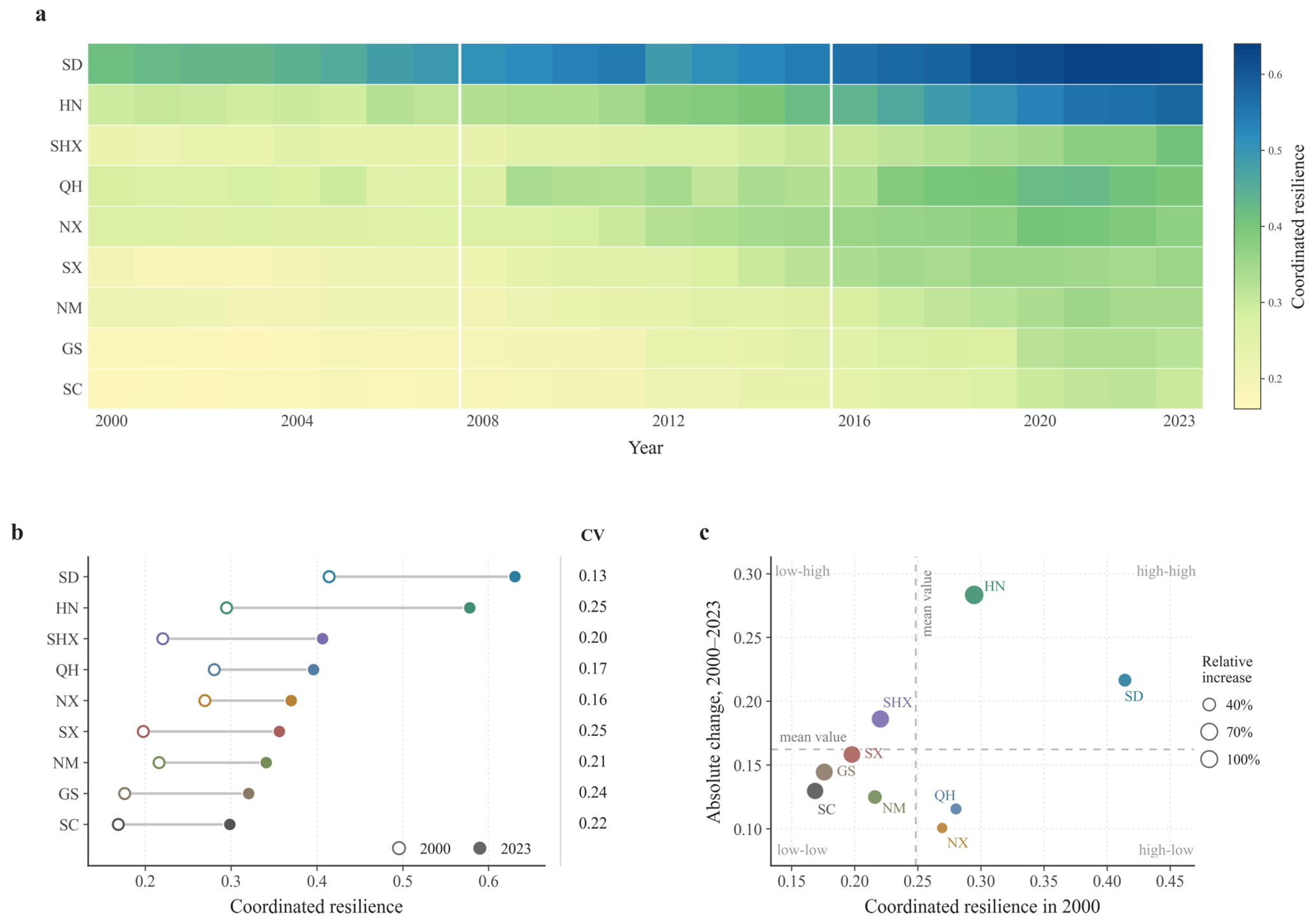
Figure 4 and Figure 5 reveal a persistent provincial hierarchy. Shandong and Henan occupied the upper end of the distribution for most years, while Gansu and Sichuan remained relatively low. The other five regions clustered mainly in the middle and changed rank more frequently. All nine regions improved, but the leading and lagging groups changed little.
Shandong recorded the highest coordinated resilience, increasing from 0.4140 in 2000 to 0.6304 in 2023. Henan gained 0.2834 and had the steepest provincial Theil–Sen slope (0.01360 yr−1). Both provinces performed relatively strongly across several subsystems, although Population remained their main internal weakness. Gansu and Sichuan ranked lowest in 2023 and showed concurrent weaknesses in Urban, Cropland, Population, and Ecology.
Among middle-ranking regions, Shaanxi rose rapidly in later years and reached 0.4064 in 2023, close to the nine-region mean. Qinghai showed greater annual fluctuation, with relatively high Population and Industry resilience but weaker Urban, Cropland, and Ecology performance. Ningxia, Shanxi, and Inner Mongolia improved more steadily, although their subsystem profiles remained less balanced than those of Shandong and Henan.
All nine provincial Theil–Sen slopes were positive. The trend was significant at p < 0.001 in eight regions and at p < 0.01 in Inner Mongolia. Shandong had the lowest temporal coefficient of variation (0.1348), consistent with its stable high-resilience series. Henan had the highest value (0.2489), reflecting its larger gain and differences across the predefined windows. Shanxi, Gansu, and Sichuan also showed relatively high temporal variability.

3.2.2. Regional Disparity Dynamics and σ-Convergence

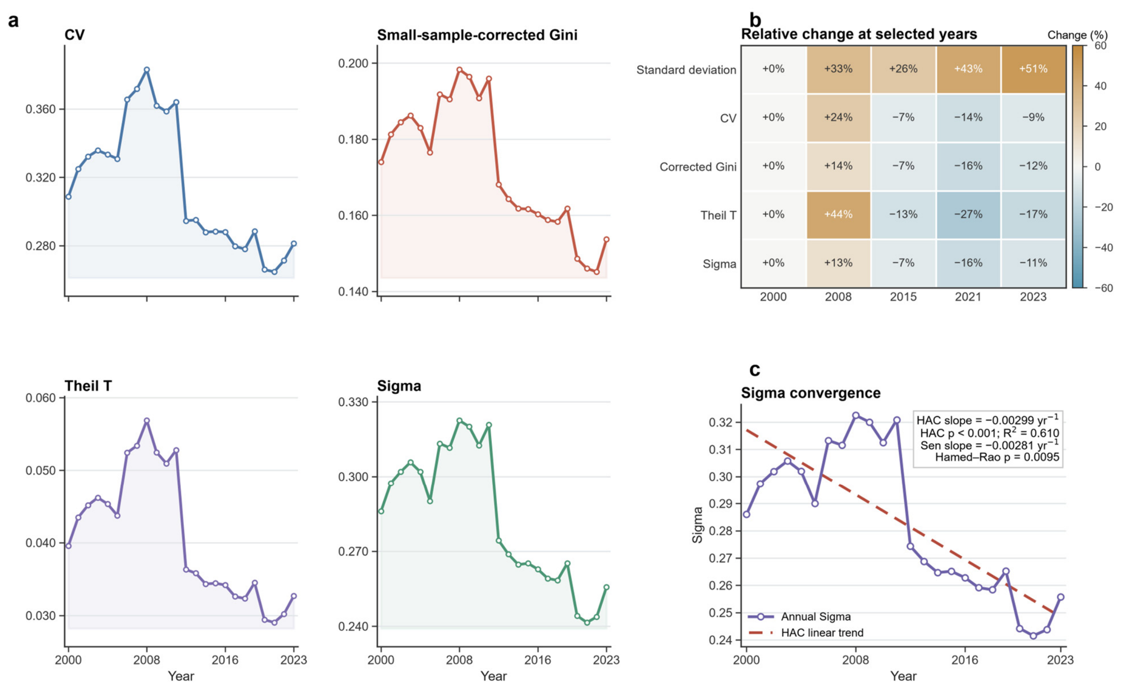
Interprovincial disparities initially widened and later declined (Figure 6). The corrected Gini coefficient increased from 0.1740 in 2000 to 0.1983 in 2008 and then fell to 0.1537 in 2023. The σ series followed a similar trajectory, rising from 0.2860 to 0.3225 before declining to 0.2557. The Theil T index and annual cross-sectional coefficient of variation changed in the same direction.
The decline in relative disparity from the second predefined window onward coincided with faster gains in Urban, Population, and Ecology resilience among several middle- and lower-resilience regions. Shandong and Henan had improved earlier from stronger initial positions, while other regions lagged during the first window. Subsequent catch-up was incomplete: Cropland resilience remained slow, and Gansu and Sichuan retained multiple subsystem weaknesses. This temporal correspondence is descriptive and does not establish a structural break or causal effect at the window boundaries.
Absolute dispersion moved differently from the relative measures. The sample standard deviation increased from 0.0767 in 2000 to 0.1155 in 2023, even as the corrected Gini coefficient, Theil T index, coefficient of variation, and σ series declined. Provincial resilience values became less dispersed relative to the rising nine-region mean but more widely separated in absolute terms.
The σ trend was negative and statistically significant (Table 3; Figure 6c). The linear coefficient was −0.00299 with a Newey–West HAC standard error of 0.00058 (p < 0.001). The Hamed–Rao test gave a Sen slope of −0.00281 (p = 0.0095). These results support relative σ-convergence over 2000–2023, although the absolute spread and broad provincial hierarchy persisted.

3.3. Structural Diagnosis of Subsystem Constraints

3.3.1. Nine-Region Structural Shortages

Relative structural shortage shares compare each subsystem with the other four within the same sample. A larger share identifies a comparatively weaker subsystem; it does not indicate that its resilience declined in absolute terms.
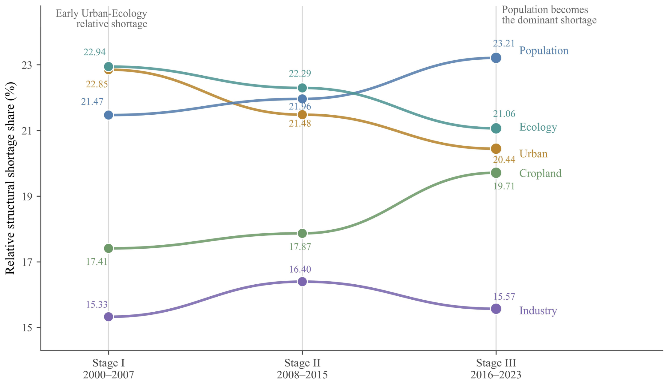
Figure 7 shows a clear change in nine-region mean shortage structure. Ecology (22.94%) and Urban (22.85%) had the largest shares in the first stage. By the third stage, Population had become the largest shortage at 23.21%, while Cropland increased from 17.41% to 19.71%. Urban declined to 20.44% and Ecology to 21.06%. Their lower shares coincided with faster resilience gains, whereas Population and Cropland improved more slowly.
Population and Cropland shortage shares increased by 1.74 and 2.30 percentage points from the first to the third stage. Urban and Ecology declined by 2.41 and 1.88 percentage points, respectively. Industry remained the smallest nine-region mean shortage, ranging from 15.33% to 16.40%. The mean subsystem coefficient of variation fell from 0.6318 to 0.4739 and 0.4048 across the three stages. The subsystem range declined from 0.4085 to 0.3743 before rising to 0.3969.
Across the nine-region panel, the dominant shortage shifted from an Urban–Ecology pattern to one led by Population, with a larger Cropland share. Urban and Ecology remained substantial constraints in the third stage, but their relative shares declined. The result is a reordering of subsystem weaknesses rather than a fixed three-subsystem ranking.

3.3.2. Provincial Transitions in Dominant Constraints

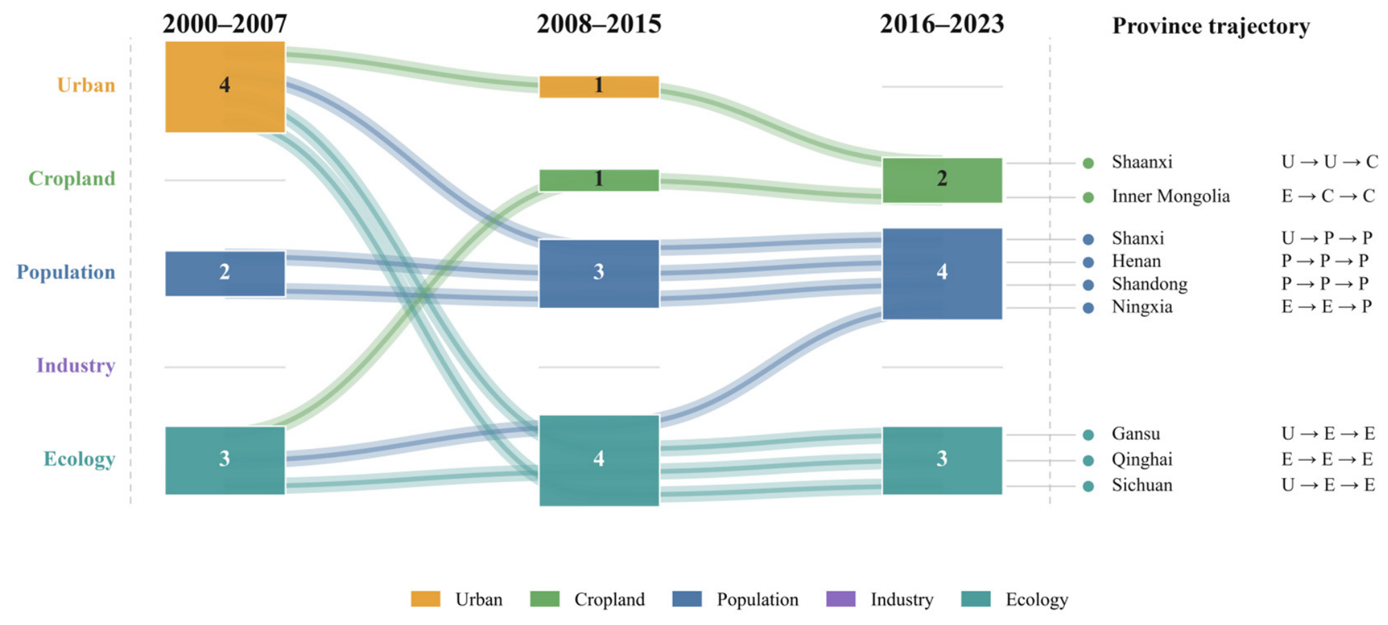
Provincial bottlenecks followed different trajectories (Figure 8). Population remained dominant in Henan and Shandong across all three stages, while Ecology remained dominant in Qinghai. The other six regions changed dominant subsystem at least once.
Henan and Shandong combined high coordinated resilience with a persistent Population bottleneck. Their Urban, Cropland, Industry, and Ecology indices were comparatively strong, leaving Population as the largest relative weakness. Population resilience itself did not decline. Its slower improvement retained pressure from population size, density, per capita water availability, domestic water use, and public-service demand.
Ecology remained Qinghai’s dominant bottleneck in all three stages. The result indicates a persistent relative weakness within its UCPIE profile. Qinghai’s ecological role, high elevation, cold climate, complex terrain, and restoration constraints may limit the pace of improvement. This interpretation concerns relative subsystem performance and does not imply ineffective environmental governance.
The remaining provinces underwent distinct transitions. Gansu and Sichuan moved from Urban in the first stage to Ecology in the second and third stages. Shaanxi shifted from Urban to Cropland, and Inner Mongolia from Ecology to Cropland. Shanxi and Ningxia moved toward Population bottlenecks in later stages. The later Cropland and Population bottlenecks are consistent with slower adjustment in irrigation, cropland allocation, groundwater dependence, population carrying capacity, and per capita resource conditions.
Dominant bottlenecks changed as subsystem improvement rates diverged. Henan, Shandong, and Qinghai showed persistent constraints, while the other provinces moved from earlier Urban or Ecology weaknesses toward Cropland or Population. The provincial results distinguish persistent from transitional bottlenecks within similar overall growth trajectories.

3.4. Indicator-Level Obstacle Factors

Indicator obstacle degrees locate the standardized gaps underlying subsystem bottlenecks. They measure relative constraints within the study sample, not absolute deterioration. Five indicators accounted for 49.59% of the total obstacle degree in the first stage: per capita water resources, effectively irrigated area, regional green coverage, industrial diversification, and built-up area. Their combined share increased to 52.71% in the second stage and 57.19% in the third.
Per capita water resources remained the largest obstacle, increasing from 11.32% to 12.33% and 14.63% across the three stages. The proportion of effectively irrigated area rose from 10.95% to 12.89%. Regional green coverage remained near 11%, industrial diversification ranged from 9.27% to 10.63%, and built-up area increased from 7.45% to 8.20%. By comparison, ecological water-use guarantee, reclaimed water utilization, and industrial water-use share declined.
Later-stage obstacles were increasingly concentrated in per capita water availability and irrigation support. Ecological spatial capacity, built-up land, and industrial diversification remained persistent constraints. The indicator pattern was consistent with the rising Population and Cropland shortage shares.

3.5. Sensitivity to Subsystem Weights

The main patterns changed little across the ten alternative weighting schemes. Spearman correlations with the baseline ranged from 0.981 to 0.996 for the 216 sample scores and from 0.989 to 1.000 for the annual nine-region mean series. Annual Theil–Sen slopes remained positive at 0.00772–0.00921 yr−1, with Hamed–Rao p < 0.001 in every scheme. All nine regions retained positive and significant trends. Spearman correlations for long-term provincial ranks ranged from 0.950 to 1.000. The composition of the bottom-three group was unchanged, while the top-three overlap ranged from two to three and the largest 2023 rank shift was two places. The upward trend and broad provincial ordering were stable, although some provinces moved by one or two places.

4. Discussion

4.1. Differentiated Subsystem Improvement During Coordinated Resilience Growth

Growth in coordinated resilience was driven mainly by Urban and Ecology, whereas Cropland changed little and Industry varied across stages. Similar improvements in urban, water-resource, and ecological resilience have been reported elsewhere in the basin [8,9,12,17,49,50,51,52]. The UCPIE comparison shows why these gains cannot be interpreted as uniform system-wide progress: subsystem trajectories remained uneven throughout the study period.
Different adjustment times may explain part of this divergence. Urban infrastructure, wastewater treatment, reclaimed water use, ecological restoration, and environmental regulation can respond relatively quickly to targeted investment. Cropland and Population are more closely tied to irrigation networks, groundwater dependence, land allocation, settlement patterns, and per capita resource availability. These conditions usually change more slowly. As Urban and Ecology improved, Population became the largest relative shortage and Cropland gained prominence. The nine-region mean index rose, but the composition of the remaining constraints changed.

4.2. Spatial Persistence Amid Relative Convergence

All nine regions improved, yet the provincial hierarchy remained stable. Shandong and Henan stayed near the top, Gansu and Sichuan near the bottom, and most rank changes occurred within the middle group. The hierarchy was not a simple upstream–downstream gradient. Source-area research has documented strong spatial heterogeneity in water-yield services [53]. Work in the Shanxi section found uneven ecosystem-service supply and demand [54], while lower-Yellow studies describe tension between concentrated socioeconomic activity and ecological protection [55].
The third-stage shortage structure further distinguishes the regions. Ecology ranked first in Qinghai, Gansu, and Sichuan, whereas Cropland led in Shaanxi and Inner Mongolia. Population was the leading shortage in Henan, Shandong, Shanxi, and Ningxia. Shandong and Henan nevertheless retained the highest coordinated-resilience levels, while Gansu and Sichuan remained lower. Provincial rank and bottleneck composition do not convey the same information. A province can score highly overall while retaining a persistent shortage, and provinces with similar scores may be constrained by different subsystems.
The decline in relative disparity reflected partial catch-up by several middle- and lower-resilience regions, while the high- and low-value groups remained broadly stable. Such persistence is consistent with the long influence of industrial structure, institutional capacity, infrastructure, and resource endowment on regional adjustment [6,7]. Relative convergence does not require provinces to reach similar index levels; it indicates that dispersion declined relative to the rising nine-region mean. The weight comparisons support the use of the equal-weight baseline for general trends and regional groupings, while individual rank positions remain weight-sensitive.

4.3. Implications for Regional Adaptive Governance Along the Yellow River

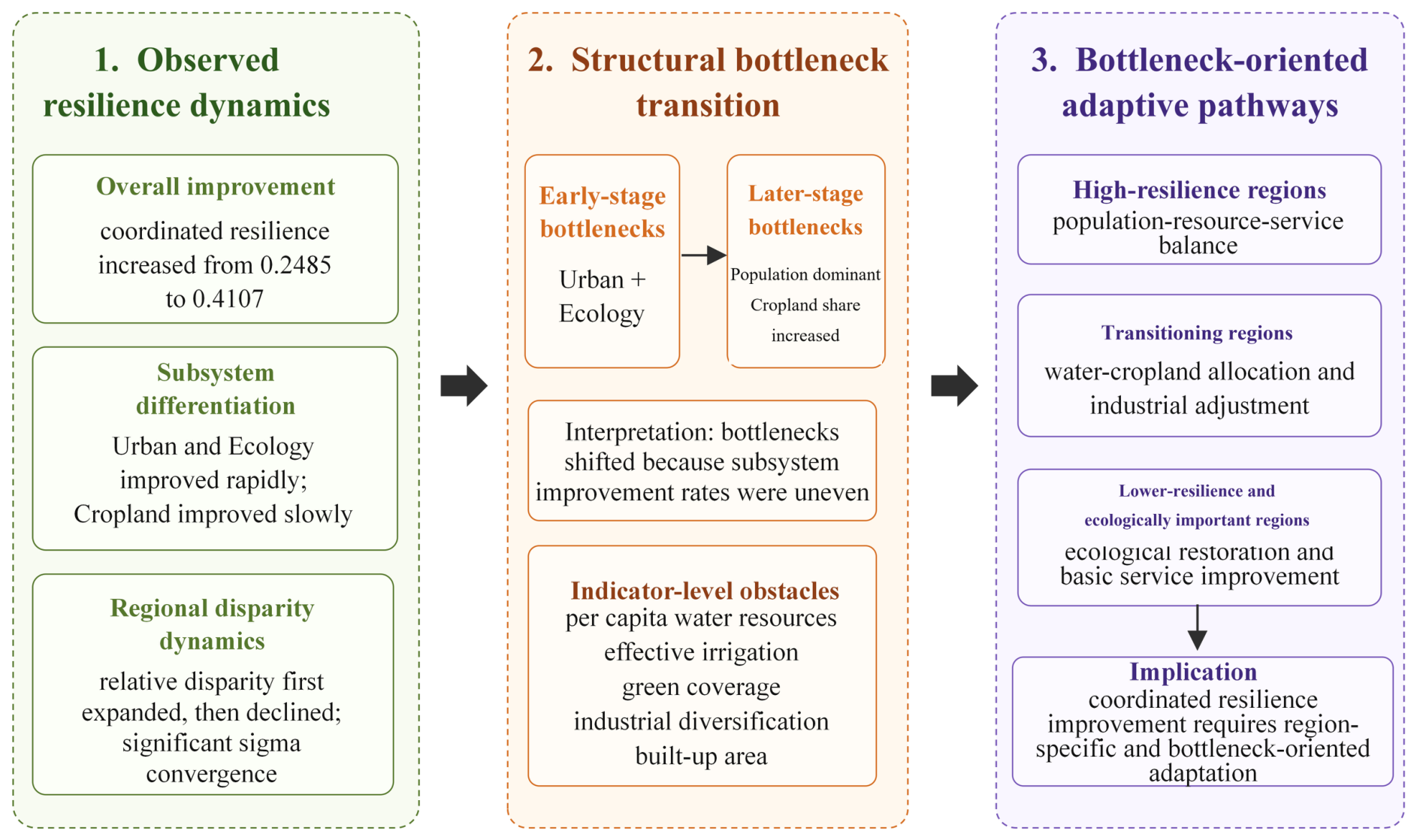
Adaptive governance should account for both the level and composition of coordinated resilience. Higher index values did not eliminate internal imbalance, and the dominant shortage changed across stages. Figure 9 links the observed trajectories and bottleneck transitions to region-specific management priorities.
Broad reach groups are useful for organizing the comparison, although each observation still represents a complete provincial unit. In the upper reaches, Qinghai’s role as an ecological water source makes ecological water allocation and source-area protection particularly relevant [53]. Gansu and Sichuan also showed Ecology shortages, whereas Inner Mongolia was constrained mainly by Cropland and Ningxia by Population. These provinces do not share a single constraint profile.
The middle reaches show a different contrast. Shaanxi’s Cropland shortage draws attention to irrigation efficiency and land allocation. Shanxi was constrained mainly by Population, particularly per capita water availability and public-service capacity. The documented mismatch between ecosystem-service supply and demand in the Shanxi section [54] also supports joint consideration of resource use and ecological functions.
Henan and Shandong remained highly ranked, but Population was their main shortage. For these downstream provinces, the main concerns are domestic and agricultural water demand, per capita resource pressure, and service efficiency. This reading is consistent with lower-Yellow evidence that dense population and agricultural activity coexist with ecological protection needs [55].
The Four Water–Four Determinations principle should be applied through the diagnosed provincial constraint profiles rather than through one basin-wide prescription.
Across the nine-region panel, coordinated resilience and relative shortage shares provide complementary monitoring signals. Annual indices reveal departures from long-term trends, while stage averages show whether dominant bottlenecks are persistent or emerging.

4.4. Scope of Interpretation and Future Research

The province-level panel is suited to comparing long-term trajectories across the nine regions, but it cannot show variation among cities, irrigation districts, or sub-basins. Because the indicators describe complete provincial units, the maps and rankings should be read as regional summaries rather than conditions at every location within the hydrological basin. Prefecture-level and sub-basin analyses could reveal whether the same hierarchy and bottleneck transitions remain visible within provinces.
The trend and obstacle results describe temporal associations and relative gaps; they do not identify what produced a change. The 24-indicator set also favors variables with consistent definitions and complete records across all regions and years, so some locally important conditions are not represented. Future studies can pair finer spatial data with process-specific designs and additional indicators where comparable long-term records are available.
Because the additive index permits stronger subsystem performance to offset weaker performance, a useful extension would compare the resulting rankings with a non-compensatory method, such as ELECTRE or PROMETHEE, or with a fuzzy aggregation rule. ANP could also extend the weighting structure when dependencies among indicators or subsystems can be specified.
The current indicator set captures long-term water availability, use intensity, irrigation efficiency, recycling, groundwater dependence, and ecological water provision. These variables are suited to tracking structural changes in provincial resilience over 2000–2023, but they do not resolve event-scale hydrological stress. Future extensions could combine the panel with drought frequency, severity, recovery time, and supply reliability, together with abstraction-to-renewable-resource ratios, sustainable abstraction thresholds, water productivity, and the ecological and chemical status of surface water and groundwater. Such additions would link long-term resilience assessment more directly to water allocation, drought preparedness, and water-body management.

5. Conclusions

This study traced the coordinated resilience of the Urban, Cropland, Population, Industry, and Ecology systems under shared water constraints in nine provincial-level regions along the Yellow River from 2000 to 2023. Overall performance, interprovincial disparity, and subsystem shortages were examined together. This approach distinguished growth in the composite index from changes in the structure beneath it.
Mean coordinated resilience rose from 0.2485 in 2000 to 0.4107 in 2023, and all nine regions followed significant upward trends. The gains were uneven across subsystems. Urban and Ecology improved rapidly, Cropland changed little, and Industry varied across stages. Interprovincial disparity widened early and later narrowed. The corrected Gini coefficient rose from 0.1740 in 2000 to 0.1983 in 2008, then fell to 0.1537 in 2023. The Sigma trend was significantly negative, indicating σ-convergence even though the absolute spread increased. Relative convergence did not erase the provincial hierarchy. Shandong and Henan remained near the top, whereas Gansu and Sichuan remained near the bottom.
The structure of the remaining shortages also changed over time. Urban and Ecology dominated the early shortage profile, whereas Population became the largest shortage in the third stage and Cropland gained weight. Provincial patterns were distinct. Ecology ranked first in Qinghai, Gansu, and Sichuan; Cropland in Shaanxi and Inner Mongolia; and Population in Henan, Shandong, Shanxi, and Ningxia. Per capita water resources and the proportion of effectively irrigated area were the largest indicator obstacles in the third stage, at 14.63% and 12.89%, respectively.
Over the study period, coordinated resilience rose and relative disparities narrowed, but structural bottlenecks persisted. The composite index alone does not show how those constraints were reordered. Under the Four Water–Four Determinations principle, adaptation measures should be matched to each province’s water constraint and subsystem profile rather than derived from a single basin-wide ranking. Work at prefecture and sub-basin scales could test whether the provincial patterns also occur within provinces.

Author Contributions

Conceptualization, X.C. and C.Z.; methodology, X.C. and C.Z.; software, X.C.; validation, P.H. and J.L.; formal analysis, X.C.; investigation, X.C.; data curation, X.C.; writing—original draft preparation, X.C.; writing—review and editing, C.Z., P.H. and J.L.; visualization, X.C.; supervision, C.Z.; project administration, C.Z. All authors have read and agreed to the published version of the manuscript.

Funding

This research was supported by the National Key Research and Development Program of China (No. 2024YFC3211304).

Institutional Review Board Statement

Not applicable.

Informed Consent Statement

Not applicable.

Data Availability Statement

The data are available from the corresponding author upon reasonable request.

Conflicts of Interest

The authors declare no conflict of interest.

Abbreviations

The following abbreviations are used in this manuscript:
CVCoefficient of Variation
GDPGross Domestic Product
HACHeteroskedasticity and Autocorrelation Consistent
NDVINormalized Difference Vegetation Index
SDStandard Deviation
TOPSISTechnique for Order Preference by Similarity to Ideal Solution
UCPIEUrban–Cropland–Population–Industry–Ecology

References

  1. Zuo, Q.; Ji, Y.; Ma, J.; Zang, C. Multilevel Evaluation Contents and Methods of the “Four Water-Four Determinations” Principle. Adv. Water Sci. 2025, 36, 744–755. [Google Scholar] [CrossRef]
  2. Zuo, Q.; Li, J.; Yu, L. Mechanism and Harmony Regulation of Human-Water Relationship in Yellow River Basin. J. Hydroelectr. Eng. 2022, 41, 1–8. [Google Scholar] [CrossRef]
  3. Wu, Q.; Zuo, Q.; Zhang, Z.; Ji, Y. A two-stage inverse intelligent path optimization model for human-water relationship regulation. Water Res. 2026, 289, 124963. [Google Scholar] [CrossRef] [Scilit] [PubMed]
  4. Holling, C.S. Resilience and Stability of Ecological Systems. Annu. Rev. Ecol. Syst. 1973, 4, 1–23. [Google Scholar] [CrossRef] [Scilit]
  5. Folke, C. Resilience: The emergence of a perspective for social-ecological systems analyses. Glob. Environ. Change 2006, 16, 253–267. [Google Scholar] [CrossRef] [Scilit]
  6. Martin, R.; Sunley, P. On the notion of regional economic resilience: Conceptualization and explanation. J. Econ. Geogr. 2015, 15, 1–42. [Google Scholar] [CrossRef] [Scilit]
  7. Pendall, R.; Foster, K.A.; Cowell, M. Resilience and regions: Building understanding of the metaphor. Camb. J. Reg. Econ. Soc. 2010, 3, 71–84. [Google Scholar] [CrossRef] [Scilit]
  8. Sun, Y.; Lu, P.; Qu, B.; Li, J. Resilience Assessment and Influencing Factors Analysis of Water Security System in the Yellow River Basin. Sustainability 2024, 16, 9347. [Google Scholar] [CrossRef] [Scilit]
  9. Li, J.; He, W.; Jiang, E.; Qu, B.; Yuan, L.; Degefu, D.M.; Ramsey, T.S. Spatio-Temporal Evaluation of Water Resources System Resilience and Identification of Its Driving Factors in the Yellow River Basin. Water 2024, 16, 414. [Google Scholar] [CrossRef] [Scilit]
  10. Wan, F.; Kang, Y.; Wang, Y.; Wang, W.; Guo, H.; Zhao, P.; Zhao, J.; Zhou, Z.; Li, M. Resilience assessment and spatiotemporal evolution analysis of water resources system in the provinces along the Yellow River. Sci. Rep. 2026, 16, 1904. [Google Scholar] [CrossRef] [Scilit] [PubMed]
  11. Yu, L.; Wu, X.; Sang, S.; Li, Y.; Li, C.; Ye, Q.; Varis, O.; Fu, B.; Wang, S. Yellow River Basin water stress has eased but may persist without enhanced efficiency and sustainable agriculture. Commun. Sustain. 2026, 1, 9. [Google Scholar] [CrossRef] [Scilit]
  12. Ji, X.; Nie, Z.; Wang, K.; Xu, M.; Fang, Y. Spatiotemporal evolution and influencing factors of urban resilience in the Yellow River Basin, China. Reg. Sustain. 2024, 5, 100159. [Google Scholar] [CrossRef] [Scilit]
  13. Li, H.; Zhu, M.; Wang, Z.; Hong, J.; Wang, Y. Synergy level of urban resilience and urban land use efficiency in the Yellow River Basin: Spatial-temporal evolution characteristics and driving factors. Heliyon 2024, 10, e31456. [Google Scholar] [CrossRef] [Scilit] [PubMed]
  14. Yu, T.; Jia, S.; Cui, X. From efficiency to resilience: Unraveling the dynamic coupling of land use economic efficiency and urban ecological resilience in Yellow River Basin. Sci. Rep. 2024, 14, 16518. [Google Scholar] [CrossRef] [Scilit] [PubMed]
  15. Yang, Z.; Cui, X.; Dong, Y.; Guan, J.; Wang, J.; Xi, Z.; Li, C. Spatio-temporal heterogeneity and influencing factors in the synergistic enhancement of urban ecological resilience: Evidence from the Yellow River Basin of China. Appl. Geogr. 2024, 173, 103459. [Google Scholar] [CrossRef] [Scilit]
  16. Li, C.; Han, H.; Cui, N.; Lan, P.; Zhang, K.; Zhou, X.; Guo, L. Spatiotemporal dynamics and spatial correlation patterns of urban ecological resilience across the Yellow River Basin in China. Sci. Rep. 2024, 14, 31286. [Google Scholar] [CrossRef] [Scilit] [PubMed]
  17. Huang, J.; Zhong, P.; Zhang, J.; Zhang, L. Spatial-temporal differentiation and driving factors of ecological resilience in the Yellow River Basin, China. Ecol. Indic. 2023, 154, 110763. [Google Scholar] [CrossRef] [Scilit]
  18. Zhang, Y.; Wang, Y. Water-Energy-Food Nexus in the Yellow River Basin of China under the Influence of Multiple Policies. Land 2024, 13, 1356. [Google Scholar] [CrossRef] [Scilit]
  19. Li, Y.; Lv, Y.; Zhang, Z.; Feng, X.; Chen, X. Coupling coordination evaluation of “Three Waters” system and impulse response analysis in the Yellow River Basin. Sustain. Cities Soc. 2024, 102, 105174. [Google Scholar] [CrossRef] [Scilit]
  20. Li, J.; Tian, G.; Wu, Z.; Niu, X.; Lou, Z.; Zhao, Q.; Xia, Q.; Zhang, J. A regionally adaptive framework for water-energy-food nexus resilience: Multi-method spatiotemporal analysis in the Yellow River Basin. Humanit. Soc. Sci. Commun. 2025, 12, 1545. [Google Scholar] [CrossRef] [Scilit]
  21. Feng, Y.; Wang, J.; Ren, X.; Zhu, A.; Xia, K.; Zhang, H.; Wang, H. Impact of water utilization changes on the water-land-energy-carbon nexus in watersheds: A case study of Yellow River Basin, China. J. Clean. Prod. 2024, 443, 141148. [Google Scholar] [CrossRef] [Scilit]
  22. Li, J.; Liu, X.; Wei, L.; Li, X.; Gao, H.; Chen, R.; Cui, Y. Investigation of the interactions and influencing factors of the Water-Land-Energy-Carbon system in the Yellow River Basin. Sci. Total Environ. 2024, 954, 176654. [Google Scholar] [CrossRef] [Scilit] [PubMed]
  23. Han, X.; Hua, E.; Cao, X.; Engel, B.A.; Sun, S.; Wang, Y. Deciphering water-energy-food synergies through a multi-level symbiosis framework: Insights from the Yellow River Basin. Agric. Syst. 2026, 231, 104531. [Google Scholar] [CrossRef] [Scilit]
  24. Yang, Z.; Li, L.; Su, Y.; Huo, L.; Yang, G. Multi-Objective Collaborative Optimization Model and Application of the Water-Energy-Food-Carbon Nexus Under Uncertainty: A Case Study of the Heihe Irrigation Area. Water 2026, 18, 841. [Google Scholar] [CrossRef] [Scilit]
  25. Yang, G.; Xia, S.; Huo, L.; Li, M.; Zhang, C.; Su, Y.; Guo, D. Two-Stage Multiobjective Decision-Making Method Based on Agricultural Water-Energy-Food Nexus: Case Study in Hetao Irrigation District, China. J. Water Resour. Plan. Manag. 2023, 149, 05023006. [Google Scholar] [CrossRef] [Scilit]
  26. Han, X.; Hua, E.; Guan, J.; Engel, B.A.; Liu, R.; Bai, Y.; Sun, S.; Wang, Y. Development of a method to assess synergy and competition for water use among water-energy-food nexus in the Yellow River Basin: Water quantity-quality dimensions. J. Hydrol. 2024, 639, 131607. [Google Scholar] [CrossRef] [Scilit]
  27. Hou, Y.; Zhao, G.; Liu, Y.; Li, X. Spatial adaptation patterns and coordinated development of water-energy-food complex system in the Yellow River Basin. Sci. Rep. 2024, 14, 31241. [Google Scholar] [CrossRef] [Scilit] [PubMed]
  28. Wu, F.; Huang, D.; He, Z.; Liu, S. Water competition and drivers for energy-food production in the Yellow River Basin under rigid water resource constraints. Agric. Water Manag. 2025, 322, 109961. [Google Scholar] [CrossRef] [Scilit]
  29. Lu, C.; Ji, W.; Hou, M.; Ma, T.; Mao, J. Evaluation of efficiency and resilience of agricultural water resources system in the Yellow River Basin, China. Agric. Water Manag. 2022, 266, 107605. [Google Scholar] [CrossRef] [Scilit]
  30. Zhang, D.; Jing, M.; Chang, B.; Chen, W.; Li, Z.; Zhang, S.; Li, T. Coordination Analysis and Driving Factors of “Water-Land-Energy-Carbon” Coupling in Nine Provinces of the Yellow River Basin. Water 2025, 17, 1138. [Google Scholar] [CrossRef] [Scilit]
  31. Lai, Z.; Li, L.; Huang, M.; Tao, Z.; Shi, X.; Li, T. Spatiotemporal evolution and decoupling effects of sustainable water resources utilization in the Yellow River Basin: Based on three-dimensional water ecological footprint. J. Environ. Manag. 2024, 366, 121846. [Google Scholar] [CrossRef] [Scilit] [PubMed]
  32. Zhang, Z.; Li, Y.; Lv, Y.; Feng, X.; Chen, X. Comprehensive evaluation of “Three Waters” carrying capacity and path evolution study: A case of the Yellow River Basin. Sci. Total Environ. 2024, 951, 175464. [Google Scholar] [CrossRef] [Scilit] [PubMed]
  33. Sui, G.; Wang, H.; Cai, S.; Cui, W. Coupling coordination analysis of resources, economy, and ecology in the Yellow River Basin. Ecol. Indic. 2023, 156, 111133. [Google Scholar] [CrossRef] [Scilit]
  34. Pang, B.; Li, X.; Fu, Y. Coupling coordination analysis and obstacle factors of water-energy-environment-economy in the Yellow River Basin. J. Clean. Prod. 2024, 468, 143108. [Google Scholar] [CrossRef] [Scilit]
  35. Wang, Z.; Liu, W. A comparative study of urban ecological resilience in the Yangtze River Economic Belt and the Yellow River Basin. Humanit. Soc. Sci. Commun. 2024, 11, 1471. [Google Scholar] [CrossRef] [Scilit]
  36. Chen, Q.; Zhu, M.; Zhang, C.; Zhou, Q. The driving effect of spatial-temporal difference of water resources carrying capacity in the Yellow River Basin. J. Clean. Prod. 2023, 388, 135709. [Google Scholar] [CrossRef] [Scilit]
  37. Cheng, X.; Bian, J.; He, D.; Tang, D. An analysis of agricultural production efficiency of Yellow River Basin based on a three-stage DEA Malmquist model. Humanit. Soc. Sci. Commun. 2025, 12, 1343. [Google Scholar] [CrossRef] [Scilit]
  38. Xiong, L.; Jiang, Y.; Li, X.; Ren, D.; Huang, G. Long-term regional groundwater responses and their ecological impacts under agricultural water saving in an arid irrigation district, upper Yellow River basin. Agric. Water Manag. 2023, 288, 108493. [Google Scholar] [CrossRef] [Scilit]
  39. Guo, L.; Song, X.; Wang, Q. Simulation of population size and economic scale supportable by the Yellow River’s available freshwater in 2030 under multiple scenarios. Humanit. Soc. Sci. Commun. 2024, 11, 26. [Google Scholar] [CrossRef] [Scilit]
  40. Feng, Y.; Zhu, A.; Liu, P.; Liu, Z. Coupling and coordinated relationship of water utilization, industrial development and ecological welfare in the Yellow River Basin, China. J. Clean. Prod. 2022, 379, 134824. [Google Scholar] [CrossRef] [Scilit]
  41. Wu, X.; Yan, Z.; Yang, H.; Wang, S.; Zhang, H.; Shen, Y.; Song, S.; Liu, Y.; Guo, Y.; Yang, D.; et al. Ecological restoration in the Yellow River Basin enhances hydropower potential. Nat. Commun. 2025, 16, 2566. [Google Scholar] [CrossRef] [Scilit] [PubMed]
  42. Hwang, C.-L.; Yoon, K. Multiple Attribute Decision Making: Methods and Applications; Springer: Berlin/Heidelberg, Germany, 1981. [Google Scholar]
  43. Mann, H.B. Nonparametric Tests Against Trend. Econometrica 1945, 13, 245–259. [Google Scholar] [CrossRef] [Scilit]
  44. Kendall, M.G. Rank Correlation Methods; Charles Griffin: London, UK, 1975. [Google Scholar]
  45. Hamed, K.H.; Ramachandra Rao, A. A modified Mann-Kendall trend test for autocorrelated data. J. Hydrol. 1998, 204, 182–196. [Google Scholar] [CrossRef] [Scilit]
  46. Deltas, G. The Small-Sample Bias of the Gini Coefficient: Results and Implications for Empirical Research. Rev. Econ. Stat. 2003, 85, 226–234. [Google Scholar] [CrossRef] [Scilit]
  47. Theil, H. Economics and Information Theory; North-Holland Publishing Company: Amsterdam, The Netherlands, 1967. [Google Scholar]
  48. Newey, W.K.; West, K.D. A Simple, Positive Semi-Definite, Heteroskedasticity and Autocorrelation Consistent Covariance Matrix. Econometrica 1987, 55, 703–708. [Google Scholar] [CrossRef] [Scilit]
  49. Li, H.; Wang, Y.; Zhang, H.; Yin, R.; Liu, C.; Wang, Z.; Fu, F.; Zhao, J. The spatial-temporal evolution and driving mechanism of Urban resilience in the Yellow River Basin cities. J. Clean. Prod. 2024, 447, 141614. [Google Scholar] [CrossRef] [Scilit]
  50. Lu, F.; Liu, Q.; Wang, P. Spatiotemporal characteristics of ecological resilience and its influencing factors in the Yellow River Basin of China. Sci. Rep. 2024, 14, 16988. [Google Scholar] [CrossRef] [Scilit] [PubMed]
  51. Chen, L.; Yu, W.; Zhang, X. Spatio-temporal patterns of High-Quality urbanization development under water resource constraints and their key Drivers: A case study in the Yellow River Basin, China. Ecol. Indic. 2024, 166, 112441. [Google Scholar] [CrossRef] [Scilit]
  52. Zhao, Y.; Zhang, H.; Man, F. Study on sustainable land use path in yellow river basin based on DSR-fsQCA approach. Discov. Sustain. 2025, 6, 1070. [Google Scholar] [CrossRef] [Scilit]
  53. Liu, M.; Zhong, J.; Xu, S. Simulation of Spatial and Temporal Variations in the Water Yield Function in the Source Area of the Yellow River and an Analysis of Influencing Factors. Sustainability 2024, 16, 8259. [Google Scholar] [CrossRef] [Scilit]
  54. Xu, M.; Feng, Q.; Zhang, S.; Lv, M.; Duan, B. Ecosystem Services Supply–Demand Matching and Its Driving Factors: A Case Study of the Shanxi Section of the Yellow River Basin, China. Sustainability 2023, 15, 11016. [Google Scholar] [CrossRef] [Scilit]
  55. Zhu, L.; Sheng, S.; Gong, H.; Yang, Q.; Zhang, X.; Xiao, H. Analyzing Coupling Coordination and Driving Factors of Social–Ecological Resilience: A Case Study of the Lower Yellow River. Sustainability 2024, 16, 10456. [Google Scholar] [CrossRef] [Scilit]
Figure 1. Analytical framework of UCPIE coordinated resilience.
Sustainability 18 08779 g001
Figure 2. Study area and spatial distribution of the nine provincial regions along the Yellow River.
Sustainability 18 08779 g002
Figure 3. Temporal evolution of UCPIE coordinated resilience and subsystem resilience across the nine provincial-level regions along the Yellow River, 2000–2023. (a) Nine-region mean coordinated resilience (black), interprovincial range (light grey), interquartile range (dark grey), and fitted linear trend (dashed); vertical lines delimit the three predefined stages. (b) Nine-region mean subsystem resilience; percentages show changes from 2000 to 2023. All subsystem panels use the same vertical scale.
Sustainability 18 08779 g003
Figure 4. Provincial heterogeneity in coordinated resilience across the nine provincial-level regions along the Yellow River. (a) Province–year resilience matrix. (b) Endpoint transitions and temporal CVs. (c) Initial resilience versus absolute gain, with bubble size indicating relative increase, dashed lines denoting cross-provincial means. Abbreviations: SD, Shandong; HN, Henan; SHX, Shaanxi; QH, Qinghai; NX, Ningxia; SX, Shanxi; NM, Inner Mongolia; GS, Gansu; and SC, Sichuan.
Sustainability 18 08779 g004
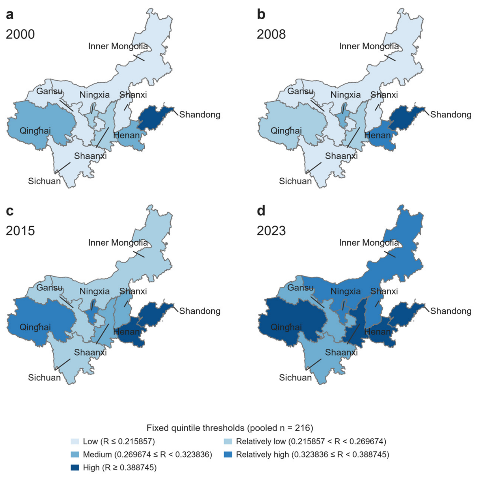
Figure 5. Spatial distribution of coordinated resilience in representative years. All four maps use the same fixed quintile thresholds derived from the pooled distribution of 216 province–year observations: 0.215857, 0.269674, 0.323836, and 0.388745.
Sustainability 18 08779 g005
Figure 6. Evolution of interprovincial disparity and σ-convergence in coordinated resilience from 2000 to 2023. (a) Annual trajectories of the coefficient of variation (CV), small-sample-corrected Gini coefficient, Theil T index, and Sigma across the nine provincial regions. (b) Percentage changes in the sample standard deviation, CV, corrected Gini, Theil T, and Sigma relative to their 2000 values for selected years; warm and cool colors indicate increases and decreases, respectively. (c) Annual Sigma series and its linear time trend estimated with Newey–West HAC standard errors (maxlags = 2); the annotation also reports the Theil–Sen slope and Hamed–Rao modified Mann–Kendall p-value.
Sustainability 18 08779 g006
Figure 7. Average relative structural shortage shares of the five UCPIE subsystems across the three stages.
Sustainability 18 08779 g007
Figure 8. Stage-wise transitions in dominant structural bottlenecks across the nine provincial regions along the Yellow River.
Sustainability 18 08779 g008
Figure 9. Adaptive governance pathways for UCPIE coordinated resilience under changing structural bottlenecks.
Sustainability 18 08779 g009
Table 1. Evaluation indicators for UCPIE subsystems.
SubsystemCodeIndicatorResilience DimensionDirection
ResistanceRecoveryAdaptation
UrbanU1Urbanization rate •+
U2Proportion of built-up area• +
U3Reclaimed water utilization rate •+
U4Wastewater treatment volume per urban resident • +
U5Green coverage rate of built-up areas• +
U6Road network density • +
CroplandC1Agricultural irrigation water intensity •−
C2Proportion of effectively irrigated area• +
C3Effective utilization coefficient of farmland irrigation water •+
C4Share of agriculture, forestry, and water affairs expenditure in general public budget expenditure • +
C5Groundwater supply dependence• −
PopulationP1Total population• −
P2Population density• −
P3Per capita GDP • +
P4Per capita water resources• +
P5Per capita disposable income • +
P6Per capita domestic water use •−
IndustryI1Proportion of industrial water use• −
I2Water use per 10,000 yuan of industrial added value •−
I3Industrial diversification index • +
EcologyE1Ecological water-use guarantee rate •+
E2Annual mean NDVI• +
E3Soil erosion control intensity • +
E4Proportion of regional green coverage area• +
• denotes that the indicator falls into the corresponding resilience dimension. “+” indicates a positive effect on system-level resilience, while “−” indicates a negative effect.
Table 2. Trend test results for coordinated resilience and five UCPIE subsystem resilience indices.
Indicator20002023Relative Increase (%)Theil–Sen SlopeHamed–Rao p-Value
Coordinated resilience0.24850.410765.280.00847<0.001
Urban resilience0.11870.4218255.240.01321<0.001
Cropland resilience0.33640.374411.280.00227<0.001
Population resilience0.20960.352868.370.00672<0.001
Industry resilience0.44820.517715.530.007380.031
Ecology resilience0.12950.3868198.600.01146<0.001
Table 3. Core results of regional disparity and σ-convergence analysis.
Test ItemResult
Time trend coefficient (b)−0.00299
Newey–West HAC standard error0.00058
t-statistic−5.180
HAC p-value<0.001
95% confidence interval[−0.00412, −0.00186]
R20.6102
Sen slope−0.00281
Hamed–Rao Z−2.593
Hamed–Rao p-value0.0095
JudgmentSignificant σ-convergence
Disclaimer/Publisher’s Note: The statements, opinions and data contained in all publications are solely those of the individual author(s) and contributor(s) and not of MDPI and/or the editor(s). MDPI and/or the editor(s) disclaim responsibility for any injury to people or property resulting from any ideas, methods, instructions or products referred to in the content.