Circular Economy Policies and Sustainable Economic Growth in Emerging Markets: A Level-2 Wavelet Decomposition with Two-Way Panel Fixed Effects

Abstract

This paper examines how circular economy (CE) policies relate to sustainable economic growth and environmental sustainability across eight major emerging economies between 2005 and 2023, with particular attention to how that relationship shifts across time horizons. Much of the existing literature has a temporal aggregation problem: short- and long-run dynamics are averaged together into a single coefficient, which can obscure the underlying relationship or, worse, produce a misleading sign. We address this by decomposing two central CE variables—renewable energy share and energy intensity—into short-, medium-, and long-term frequency components using a Level-2 discrete wavelet transform. Each component is then estimated via two-way fixed-effects panel regressions; given the constraints of a relatively small panel, we validate inference using a Wild Cluster Bootstrap procedure. Three findings stand out. First, although the growth elasticity of renewable energy rises across horizons—a descriptive pattern consistent with short-run adjustment costs giving way to longer-run sustainable gains—Wild Cluster Bootstrap (WCB) inference indicates that these structural coefficients are not statistically significant in this sample. Second, the energy intensity coefficient reverses the sign, moving from a weakly significant negative short-run effect (p < 0.10) to positive estimates in the longer run; these longer-run effects, however, fail to reach statistical significance, and so offer only suggestive theoretical alignment with the macroeconomic Jevons Rebound Effect rather than firm empirical confirmation of it. Third, Industry Value Added stands out as the one robust macroeconomic factor in the model, remaining a significant and positive driver of sustainable development at every frequency horizon. Taken together, these results suggest that while CE transitions display suggestive multi-horizon dynamics, industrial expansion remains the more statistically dependable engine of sustainable growth across these emerging markets. Although statistical significance is dependent on the sample size, the identified trajectories provide a useful structural diagnosis for policymakers who need to plan different investment horizons for the sustainable green transition.

1. Introduction

The circular economy (CE) is a systemic framework that decouples economic output from virgin resource throughput by recirculating materials, recovering embodied energy, and substituting fossil-fuel inputs with renewable sources [1,2]. Over the past decade, it has moved from a theoretical proposition to an active policy agenda across both advanced and emerging economies [3,4]. Yet as nations increasingly build CE principles into their development strategies, one basic empirical question stays open: what are the quantitative macroeconomic effects of CE policy adoption on economic growth, and do those effects vary systematically across time horizons?

That question is not trivial, because theory sharply predicts different mechanisms at different temporal scales. In the short run, CE transitions, particularly large-scale renewable energy deployment, impose adjustment costs: capital reallocation away from consumption and conventional investment, grid integration expenses, fossil-fuel sector disruption, and institutional reconfiguration costs that together suppress contemporaneous output [5,6]. In the long run, the same policies generate structural productivity gains: lower marginal energy costs, reduced fossil-fuel import dependence, and technological spillovers that raise total factor productivity [7,8]. Standard panel fixed-effects estimators produce a single time-horizon-invariant coefficient, which necessarily conflates these opposed short- and long-run mechanisms into a weighted average that is ambiguous in sign, unstable across sample windows, and potentially misleading for policy design. We call this temporal aggregation bias.

The recent literature increasingly points to the structural hurdles emerging economies face in financing green infrastructure, underscoring the need for policy frameworks that account for multiple time horizons—particularly as global circularity rates remain stubbornly low [9,10].

Over the past decade, energy demand across developing and emerging economies has climbed sharply, driven by rapid industrialization, population growth, and the accelerating pace of urbanization. As these economies modernize, their energy consumption has pulled well ahead of the global average, and they now account for the bulk of new energy demand worldwide. This is not simply a statistical anomaly; it reflects a structural feature of the current growth phase, one that makes the case for integrating circular economy policies increasingly difficult to ignore. When such interventions are absent, continued economic development risks entrenching fossil-fuel dependence further, compounding environmental degradation rather than easing it.

The selection of these eight specific nations is deliberate; they are not only highly representative of emerging markets in terms of surging resource consumption and rapid urbanization, but they also serve as the primary drivers of future global energy demand. To ensure that our empirical estimates are not distorted by the volatility or revisions typical of national statistical reporting in these regions, our analysis strictly relies on harmonized, heavily vetted data series from the World Bank and the International Energy Agency (IEA).

We work around this with a Level-2 wavelet decomposition framework. Wavelet analysis, introduced to economics by Ramsey and Lampart [11] and extended to energy economics by Aguiar-Conraria et al. [12] and Jammazi and Aloui [13], decomposes a time series into components at distinct frequency scales without losing temporal localization, which is a real advantage over classical Fourier approaches. Applied at Level 2 with the Daubechies (db2) filter, the decomposition yields three orthogonal components: D₁ (short-run, 2–4 years), D₂ (medium-run, 4–8 years), and A₂ (long-run structural trend). These feed into two-way fixed-effects panel regressions with country-clustered standard errors, correcting simultaneously for cross-sectional dependence and heteroskedasticity [14,15]. Level-2 methods improve on Level-1 wavelet methods because it cleanly separates medium-run policy implementation dynamics, such as the investment payback period of a typical renewable installation or the lag between policy announcement and capacity commissioning, from both short-run cyclical shocks and decade-scale structural trends.

A second contribution concerns energy intensity. The prior literature chalks up its empirical ambiguity to measurement conflation of technological efficiency improvements, structural deindustrialization, and cyclical demand variation [4,7]. In our view, there is a more precise interpretation: the sign reversal of the energy intensity coefficient from −15.287 at D₁ to positive values at D₂ (+5.504) and A₂ (+0.787) is the empirical signature of the macroeconomic Jevons Rebound Effect [16]. Efficiency improvements lower the unit cost of energy services, which stimulates additional demand at lower frequencies, enough to dominate the aggregate energy intensity reduction. As far as we know, this is the first multi-frequency panel documentation of the macroeconomic Jevons pattern across a diverse set of emerging economies.

A central contribution of this study is methodological: it reframes the debate around the CE–growth nexus. Rather than trying to isolate universally significant, long-run elasticity coefficients (a notoriously hard task in macroeconomic panels with short time horizons), we offer a structural diagnosis of why the existing literature disagrees so much. Specifically, we show that much of that disagreement is symptomatic of temporal aggregation bias. Using a Level-2 wavelet decomposition, we provide a proof-of-concept study for how short-term cyclical contractions, medium-term implementation lags, and long-term structural dividends operate at the same time but obscure each other in standard, single-frequency estimators. The directional trajectories we identify here should be useful as a diagnostic framework for future energy economics research.

In sum, the paper makes four contributions. It introduces Level-2 wavelet panel regression as a way to resolve temporal aggregation bias in CE–growth analyses. It documents a steadily improving renewable energy–growth relationship across frequency bands, which helps reconcile apparently contradictory findings in the literature: different studies, it turns out, may simply be estimating different frequency-band effects of the same underlying process. It provides the first wavelet-based panel documentation of the macroeconomic Jevons Rebound Effect in a multi-country emerging-economy context. And it contributes rigorous econometric evidence from eight diverse emerging markets that together represent roughly 3.4 billion people and $14 trillion in GDP (2023).

The rest of the paper is organized as follows. Section 2 reviews the theoretical and empirical literature. Section 3 develops the four research hypotheses. Section 4 describes data and methodology. Section 5 presents empirical results. Section 6 works through the discussion. Section 6 draws out policy implications, and concludes the paper.

2. Literature Review

2.1. Circular Economy: Macroeconomic Channels

The circular economy draws together industrial ecology [17], cradle-to-cradle design [18], and natural capitalism [19]. The Ellen MacArthur Foundation [9] codified it as a systemic alternative to the linear ‘take-make-dispose’ model. Its macroeconomic growth channels include lower marginal energy production costs as renewable capacity matures, reduced fossil-fuel import expenditure, technological spillovers from clean energy R&D, and energy access expansion in rural areas that broadens the economically active labor force. Against these benefits, the transition phase brings costs of its own: capital reallocation, grid reliability risk from variable renewable integration, and labor market disruption in fossil-fuel-dependent regions [6]. These opposed short- and long-run mechanisms are exactly why frequency-specific estimation makes sense here.

Furthermore, in the specific context of emerging economies, the transition requires ‘patient capital.’ [20] However, political instability and short electoral cycles frequently compel local authorities to prioritize immediate, short-term interventions (D₁) over long-term structural dividends (A₂), further complicating the policy landscape.

2.2. Renewable Energy and Growth: Multi-Horizon Evidence

Before turning to the macroeconomic impacts, it is worth establishing the compositional hierarchy of renewable energy sources across emerging markets. Hydropower has historically dominated this mix, at times accounting for 50 to 60 percent of renewable capacity in countries such as Brazil and Colombia. In recent years, however, solar photovoltaic and wind power have emerged as the fastest-growing segments of new capacity additions—a shift that is driving much of the structural transition observed in economies like India and Morocco.

The empirical literature on the renewable energy–growth nexus is extensive, but its estimates differ significantly, partly because of temporal aggregation bias. Panel Granger causality studies [5] report bidirectional causality between renewable consumption and GDP. Ozcan and Ozturk’s [21] meta-analysis found that positive long-run effects predominate while short-run effects are frequently negative or insignificant.

Using Pooled Mean Group (PMG) estimation [22] across 24 African countries, we document a significantly positive long-run renewable-growth effect alongside an insignificant short-run coefficient—a pattern that aligns closely with our D₁ and A₂ findings. This is consistent with Nathaniel and Khan [23], who confirmed positive long-run renewable-growth linkages for ASEAN economies. Furthermore, wavelet-based energy-growth studies [12,13] demonstrate that energy GDP co-movement varies across time frequencies. To the best of our knowledge, no prior study has yet applied a Level-2 wavelet panel framework to clean energy (CE) variables across a multi-country emerging-economy sample.

2.3. The Jevons Rebound Effect: Theory and Panel Evidence

William Stanley Jevons [16] was the first to document that improvements in steam engine coal efficiency led to more, not less, aggregate coal consumption: lower unit costs made coal-powered production economically attractive at scales that had previously been unprofitable. The macroeconomic rebound effect generalizes this: lower energy service costs cut production costs economy-wide, which stimulates output growth and total energy demand [4]. Saunders [24] worked out the conditions under which ‘backfire’ (rebound exceeding 100 percent) is theoretically possible in a neoclassical production framework. Empirically, Sorrell [4] puts UK economy-wide rebound at 26–56 percent; Roy [25] documents significant rebound in India; and Turner [26] finds backfire conditions in Chinese manufacturing. Econometrically, the Jevons mechanism implies energy intensity should carry a positive growth coefficient at low frequencies: efficiency improvements lower energy service costs, which stimulates output growth. This in turn raises total energy demand and partially or fully offsets the efficiency gain in the aggregate energy/GDP ratio. Thus, a positive low-frequency coefficient coexists with a negative high-frequency coefficient driven by cyclical GDP contraction: precisely the sign reversal pattern we document.

2.4. Two-Way Fixed Effects and Econometric Strategy

Standard entity fixed-effects estimators absorb time-invariant cross-sectional heterogeneity but remain vulnerable to cross-sectional dependence from simultaneous global shocks [27]. Two-way fixed effects absorb both entity and time heterogeneity, which substantially cuts down cross-sectional dependence. Country-clustered standard errors give consistency under arbitrary within-country serial correlation [14]. This specification is the best practice in consensus for short balanced panels facing simultaneous macroeconomic shocks [27]. One caveat worth flagging is the following: year dummies absorb common time trends in the regressors, including the global post-2015 trend of declining renewable energy costs, which reduces the residual variation available for identifying the renewable energy coefficient, a mechanism we return to in Section 6.

2.5. Control Variables: Theoretical Rationale

Trade openness captures technology diffusion and knowledge spillovers from integration into global value chains [28]; its conditional sign turns ambiguous once global trade liberalization trends are removed [29]. FDI provides capital augmentation and productivity spillovers, with magnitudes depending on host-country absorptive capacity [30]. Urbanization proxies agglomeration economies and labor market depth [8]. Industrial Value Added captures the manufacturing-led development channel [31]. Domestic credit proxies financial depth and is subject to the ‘too much finance’ threshold [32]. Public debt proxies fiscal space, which is subject to the crowding-out of private investment [32].

3. Research Hypotheses, Data, and Methodology

3.1. Research Hypotheses

We derive four testable hypotheses from this theoretical framework:

H1 (Green Transition Cost Hypothesis). 

Renewable energy expansion exerts a negative short-run (D₁) effect on GDP growth, reflecting upfront capital reallocation costs, grid integration expenses, and fossil-fuel sector displacement.

H2 (CE Structural Dividend Hypothesis). 

Renewable energy expansion exerts a positive long-run (A₂) effect on GDP growth, as energy cost reductions, reduced import dependence, and technological spillovers accumulate structurally over time.

H3 (Jevons Rebound Hypothesis). 

Energy intensity exhibits a negative short-run (D₁) coefficient, driven by a cyclical GDP contraction that mechanically raises the energy/GDP ratio, but which has positive medium-run (D₂) and long-run (A₂) coefficients, as efficiency improvements reduce energy service costs and stimulate additional demand that partially or fully offsets the efficiency gain at these lower frequencies.

H4 (Methodological Validity Hypothesis). 

Level-2 wavelet decomposition reveals three distinct frequency-specific dynamics for CE variables that are fundamentally obscured by Level-1 decomposition and standard single-frequency panel estimators.

In summary, although the theoretical mechanisms behind green transition costs and the Jevons Rebound Effect are well documented individually, the empirical literature has yet to offer a unified framework capable of observing them simultaneously. This paper addresses this gap by applying a multi-frequency decomposition framework to circular economy variables in an emerging-economy context, thereby resolving the temporal aggregation bias that limits current single-frequency estimates.

3.2. Sample, Variables, and Sources

Though restricted to eight economies, the panel’s composition is deliberate and goes beyond mere data availability. Together, these nations form a critical bloc for the global green transition, accounting for nearly 3.4 billion people and $14 trillion in GDP in 2023. They also work as useful benchmark cases, spanning a broad range of institutional environments, economic structures, and starting renewable energy capacities. Analyzing this group gives us insights into the macroeconomic mechanics of CE transitions that should scale to emerging markets more broadly.

The dataset is a balanced panel with a total sample size of N times T = 152 observations, comprising N = 8 emerging economies over T = 19 annual periods (2005–2023). Country selection followed three criteria: emerging or developing economy classification by the IMF at the start of the sample; geographic and developmental diversity to support external validity; and complete data availability for all nine variables across the full sample period. The sample captures substantial variation in renewable energy endowments, industrial structures, and institutional environments. Data was derived from the World Bank World Development Indicators (WDI), the International Energy Agency (IEA) [33], and the IMF World Economic Outlook (WEO).

Table 1. Variable definitions, measurement units, expected signs, and data sources.

Variable	Definition	Unit	Role	Exp. Sign	Source
GDP Growth	Annual real GDP growth rate (%)	%	Dependent	—	WB WDI
Renewable Share	Renewable energy as % of total final energy consumption	%	CE Proxy (H1, H2)	±	IEA/WDI
Energy Intensity	Energy consumption per unit of real GDP output	MJ/USD	CE Proxy (H3)	−/+	IEA
FDI	Net foreign direct investment inflows	% GDP	Control	+	WB WDI
Trade Openness	(Exports + Imports)/GDP	% GDP	Control	−/+	WB WDI
Urbanization	Share of population residing in urban areas	%	Control	+	WB WDI
Industry VA	Industrial value added (manufacturing, mining, utilities)	% GDP	Control	+	WB WDI
Domestic Credit	Private sector credit extended by domestic banks	% GDP	Control	±	WB WDI
Public Debt	General government gross debt	% GDP	Control	−	IMF WEO

Notes: CE = circular economy. ± for renewable share: theory predicts a negative short-run coefficient (H1, Green Transition Cost) and a positive long-run coefficient (H2, CE Structural Dividend). −/+ for energy intensity: theory predicts a negative short-run cyclical coefficient and positive medium- and long-run coefficients consistent with the Jevons Rebound Effect (H3). WDI = World Development Indicators; IEA = International Energy Agency; IMF WEO = World Economic Outlook.

presents complete variable definitions, units, expected signs, and sources;

Table 2. Descriptive statistics.

Variable	N	Mean	SD	Min	p25	Median	Max
GDP Growth (%)	152	4.05	3.33	−7.30	2.50	4.40	11.40
Renewable Share (%)	152	25.63	12.34	6.70	15.38	24.00	46.50
Energy Intensity (MJ/USD)	152	3.65	0.60	2.70	3.30	3.60	5.40
FDI (% GDP)	152	2.63	1.54	−0.30	1.60	2.25	8.40
Trade Openness (%)	152	51.28	18.18	23.30	37.48	48.75	103.60
Urbanization (%)	152	61.20	17.03	29.40	43.88	62.90	88.70
Industry VA (% GDP)	152	30.58	5.34	19.50	27.70	29.70	42.70
Domestic Credit (% GDP)	152	52.47	17.83	22.60	38.00	52.55	93.50
Public Debt (% GDP)	152	61.13	24.08	24.50	39.23	62.05	117.20

Notes: N = 152 balanced country-year observations across eight emerging economies, 2005–2023. Zero missing observations confirmed. SD = standard deviation; p25 = 25th percentile.

and

Table 3. Country-level sample means, 2005–2023.

Country	GDP Growth (%)	Renew. Share (%)	Energy Intensity	FDI (% GDP)	Dom. Credit (% GDP)	Pub. Debt (% GDP)
Brazil	2.11	42.80	3.62	3.01	53.55	76.28
Colombia	3.77	40.11	2.91	4.96	46.14	49.52
Egypt	4.51	10.59	3.91	3.28	33.34	104.07
India	6.75	31.32	3.48	2.01	49.33	76.10
Indonesia	4.96	34.61	3.74	1.76	32.98	32.35
Morocco	3.24	12.61	3.44	3.02	72.12	61.29
South Africa	1.92	17.25	4.85	1.44	71.55	49.01
Turkey	5.13	15.73	3.23	1.58	60.73	40.38
Panel Mean	4.05	25.63	3.65	2.63	52.47	61.13

Notes: Panel mean = unweighted mean across all 152 observations. Energy intensity in MJ per constant 2017 USD of GDP.

present descriptive statistics and country-level means, respectively.

Although the circular economy (CE) encompasses a broad range of material flows and waste cycles, we use renewable energy share and energy intensity as our primary macroeconomic proxies. This choice reflects the fact that the CE transition, at the macro level, depends fundamentally on two processes: decoupling economic output from virgin fossil-fuel throughput, captured here by the expansion of renewable energy, and improvements in systemic resource efficiency per unit of output, captured by energy intensity.

3.3. Level-2 Daubechies Wavelet Decomposition

The discrete wavelet transform (DWT) at decomposition Level 2, utilizing the Daubechies (db2) mother wavelet [34,35], decomposes a given time series into three distinct and orthogonal components:

x(t) = A₂ (t) + D₂ (t) + D₁(t)

Rather than being mere statistical artifacts, each component translates directly into a specific economic horizon.

Short-Run Component (D1): This captures high-frequency, 2–4-year business-cycle fluctuations. Economically, this reflects year-to-year volatility such as policy announcement effects, cyclical energy demand swings, and grid integration shocks.

Medium-Run Component (D2): This captures 4–8-year dynamics. This aligns with the implementation and payback cycles of utility-scale renewable projects (like solar and wind), as well as medium-term labor market adjustments.

Long-Run Component (A2): This represents the decade-scale structural trend. This reflects the slow, persistent evolution of an economy’s energy mix and overall energy productivity, shaped by technological upgrading and structural change.

3.4. Two-Way Fixed-Effects Panel Estimation

It is important to note that unobserved global uncertainties, such as international armed conflicts or supply-chain disruptions affecting renewable energy materials, are systematically accounted for and absorbed by the year fixed effects λt. Meanwhile, localized uncertainties and country-specific disruptions are captured within the idiosyncratic error term εit.

For each frequency band h ∈ {D₁, D₂, A₂}, we estimate the following:

$${\mathit{Y}}_{\mathit{i}\mathit{t}}={\mathit{\alpha }}_{\mathit{i}}+{\mathit{\lambda }}_{\mathit{t}}+{\mathit{\beta }}_{\mathbf{1}}{\mathit{R}\mathit{E}}_{\mathit{i}\mathit{t}}^{\mathit{h}}+{\mathit{\beta }}_{\mathbf{2}}{\mathit{E}\mathit{I}}_{\mathit{i}\mathit{t}}^{\mathit{h}}+{\mathit{\gamma }}^{\prime }{\mathit{Z}}_{\mathit{i}\mathit{t}}+{\mathit{\epsilon }}_{\mathit{i}\mathit{t}}$$

where ${\mathit{Y}}_{\mathit{i}\mathit{t}}$ is the GDP growth rate for country i in year t; αi represents the country fixed effects absorbing all time-invariant heterogeneity (resource endowments, institutional quality, geography, and legal systems); ${\mathit{\lambda }}_{\mathit{t}}$ represents the year fixed effects absorbing all common time shocks simultaneously affecting all panel units, including the 2008–09 Global Financial Crisis, the 2014–16 commodity price collapse, the COVID-19 pandemic (2020), and the severe energy supply-chain disruptions caused by the war in Ukraine (2022–2023), and the global post-2015 trajectory of declining renewable energy technology costs; ${\mathit{R}\mathit{E}}_{\mathit{i}\mathit{t}}^{\mathit{h}}$ and ${\mathit{E}\mathit{I}}_{\mathit{i}\mathit{t}}^{\mathit{h}}$ are the wavelet-decomposed renewable energy share and energy intensity at frequency band h; ${\mathit{Z}}_{\mathit{i}\mathit{t}}$ is the vector of six time-varying control variables; and ${\mathit{\epsilon }}_{\mathit{i}\mathit{t}}$ is the idiosyncratic error term. Standard errors are clustered at the country level, providing asymptotic consistency under arbitrary patterns of within-country serial correlation and any cross-sectional dependence not absorbed by year fixed effects [14]. The two-way FE estimator is identified from within-country, within-year variation in the wavelet-decomposed CE components, with variation orthogonal to both country structural heterogeneity and common time trends. All models are estimated using linear models and the panel OLS estimator [36].

We restricted the wavelet decomposition to the circular economy variables, ${\mathit{R}\mathit{E}}_{\mathit{i}\mathit{t}}^{\mathit{h}}$ and ${\mathit{E}\mathit{I}}_{\mathit{i}\mathit{t}}^{\mathit{h}}$, in order to isolate the frequency-specific channels through which they operate. The control variables ${\mathit{Z}}_{\mathit{i}\mathit{t}}$ and year fixed effects ${\mathit{\lambda }}_{\mathit{t}}$ are retained in their raw form. This choice reflects two considerations: it allows us to control for standard macroeconomic baselines and common global shocks, and it avoids decomposing variables for which such treatment is neither necessary nor theoretically motivated.

4. Empirical Results and Robustness Inference

4.1. Main Regression Results and Wild Cluster Bootstrap Adjustments

Table 4. Main results: Three-horizon two-way fixed-effects wavelet panel regression.

Variable	Short-Run (D1)			Medium-Run (D2)			Long-Run (A2)
	Coef.	SE	p-Value	Coef.	SE	p-Value	Coef.	SE	p-Value
Renewable Share (wavelet)	−0.458	0.799	0.568 [WCB: NS]	−0.083	0.732	0.910 [WCB: NS]	0.055	0.131	0.678 [WCB: NS]
Energy Intensity (wavelet)	−15.287	7.791	0.052 * [WCB: 0.082+]	5.504	4.517	0.225 [WCB: NS]	0.787	1.510	0.603 [WCB: NS]
FDI	0.477	0.191	0.014 *	0.500	0.194	0.011 *	0.523	0.218	0.018 *
Trade Openness	−0.071	0.032	0.027 *	−0.069	0.037	0.066 *	−0.062	0.034	0.070 *
Urbanization	−0.086	0.106	0.418	−0.068	0.099	0.494	−0.010	0.092	0.917
Industry VA	1.048	0.229	<0.001 *** [WCB: p < 0.01 *] **	1.070	0.222	<0.001 *** [WCB: p < 0.01 *] **	1.081	0.228	<0.001 *** [WCB: p < 0.01 *] **
Domestic Credit	−0.013	0.035	0.718	−0.018	0.036	0.625	−0.023	0.035	0.508
Public Debt	0.008	0.030	0.781	0.005	0.030	0.868	−0.005	0.032	0.867
Constant	−20.171	10.492	0.057 *	−21.670	10.083	0.034 *	−29.322	10.289	0.005 **
Entity FE	Yes			Yes			Yes
Time FE	Yes			Yes			Yes
SE Clustering	Country			Country			Country
R2 (within)	0.2552			0.2108			0.2105
F-stat (pooled)	7.741 p < 0.001			7.744 p < 0.001			7.625 p < 0.001
N	152			152			152

Note: Significance levels (* p < 0.05, ** p < 0.01, *** p < 0.001) reflect conventional country-clustered standard errors. [WCB: …] indicates the robustness inference using the Wild Cluster Bootstrap procedure. Exact p-values or significance thresholds (NS = not significant, p < 0.10) are provided for the primary circular economy variables and key structural drivers are as discussed in Section 4.

presents the three-horizon regression results. The baseline models use a two-way fixed-effects estimator with conventional country-clustered standard errors, but our macroeconomic panel is constrained by a small number of clusters (N = 8 emerging economies), and under those conditions, conventional clustered standard errors tend to over-reject the null hypothesis. So, we supplemented the baseline p-values with a Wild Cluster Bootstrap (WCB) procedure (imposing the null hypothesis with Rademacher weights and 2000+ replications) and treated the WCB p-values as the ones that mattered for hypothesis assessment.

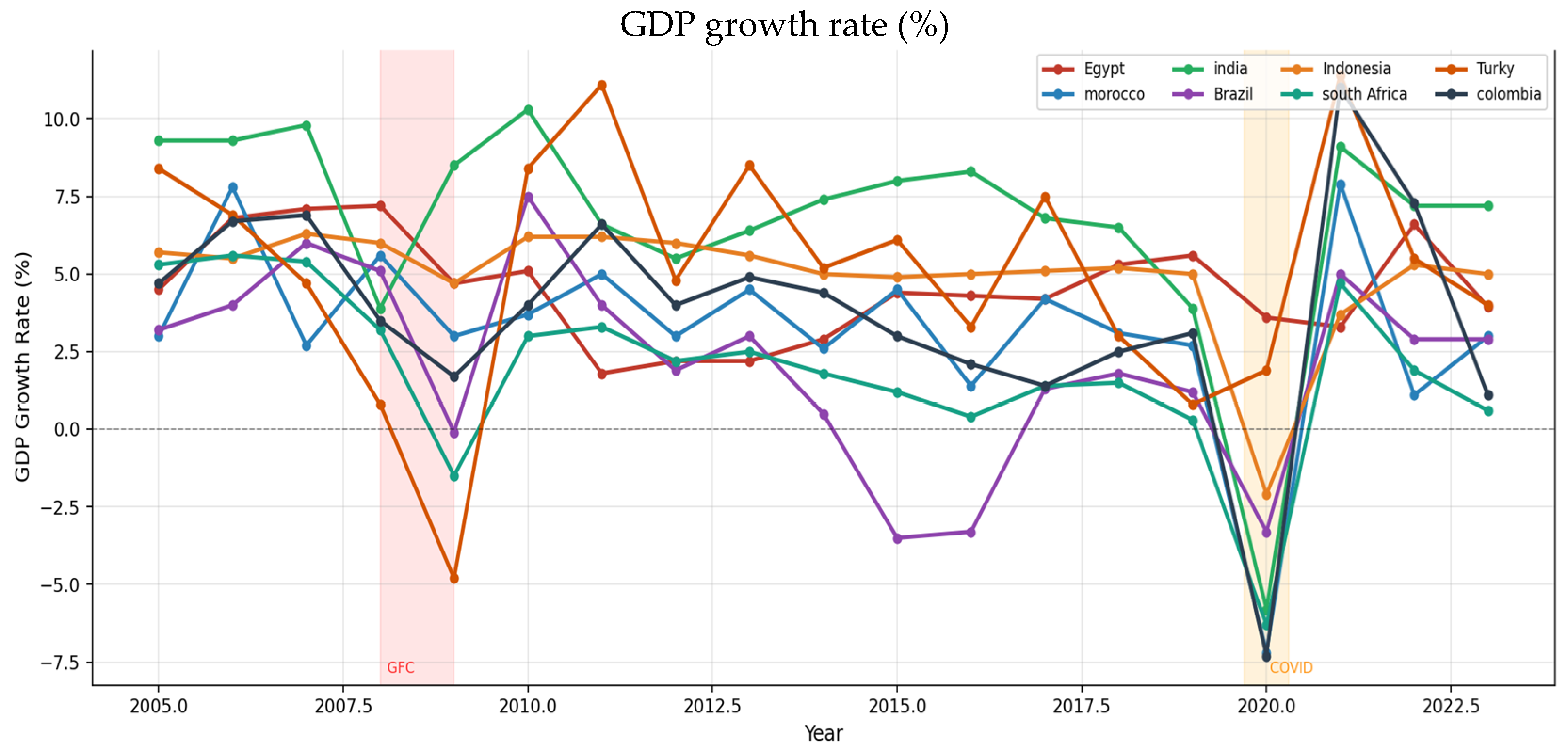
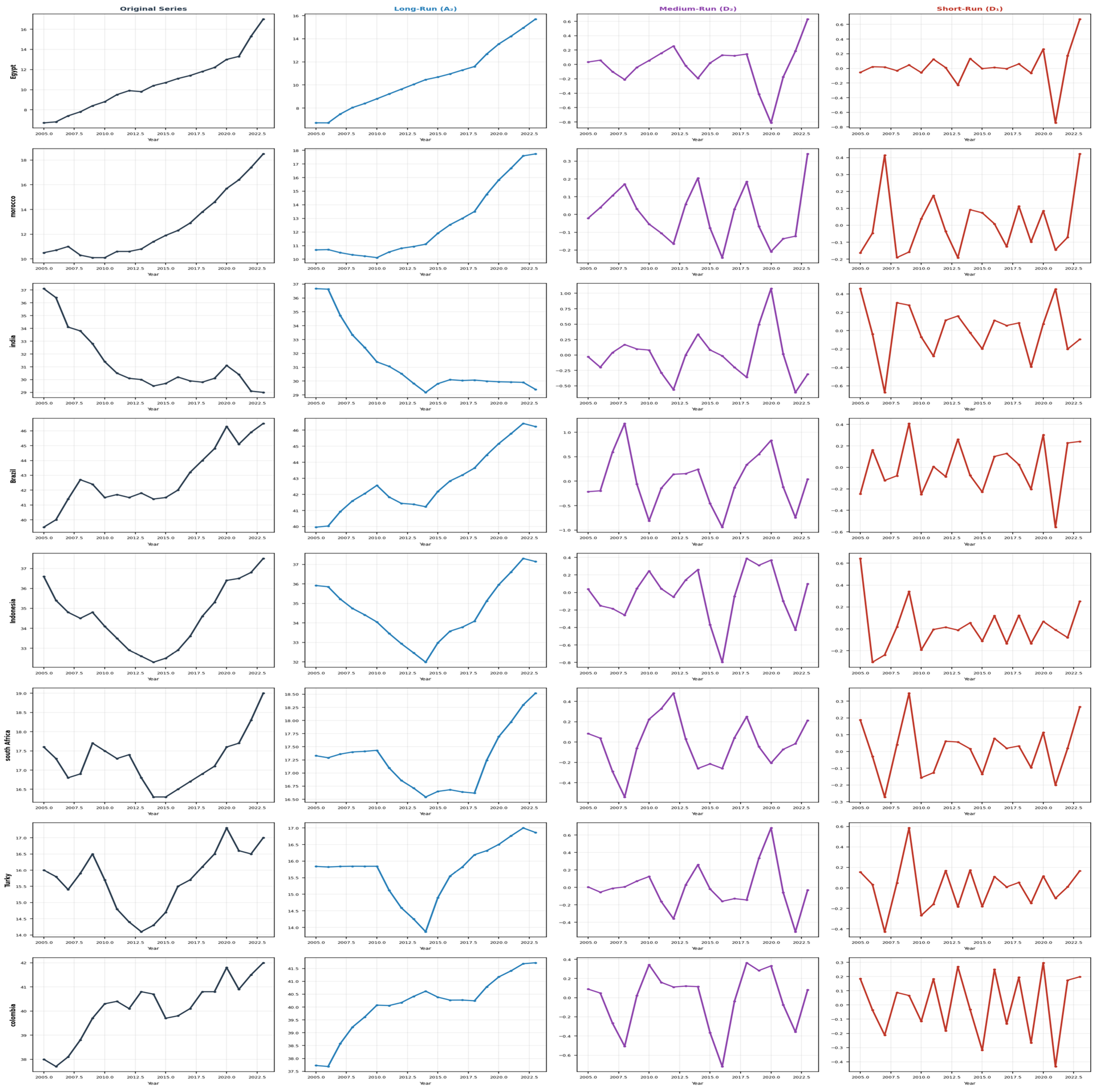
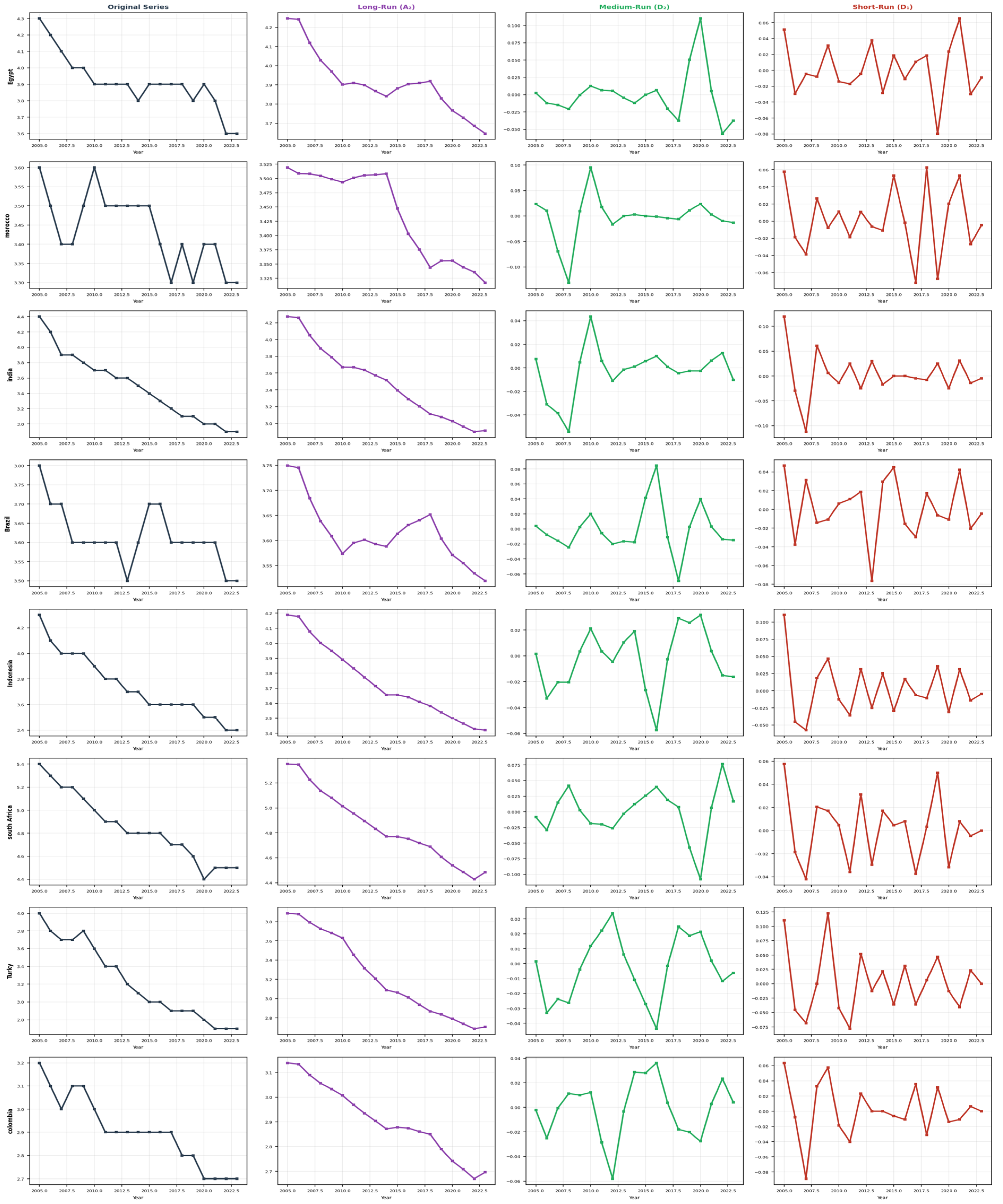
Figure 1, Figure 2 and Figure 3 present the macroeconomic growth trends and the full Level-2 db2 wavelet decompositions of the CE variables across all countries.

As shown in both the original series and the wavelet decomposition figures (Figure 1, Figure 2 and Figure 3), the resulting curves display several distinct minima and maxima. These fluctuations, most pronounced in the short-run D1 component, correspond closely to business cycle turning points and the localized effects of major global shocks. The shared global magnitude of events such as the 2008 financial crisis, the COVID-19 pandemic, and the war in Ukraine is absorbed by our year fixed effects λt; what drives the sharp peaks and troughs at this high-frequency band, however, is down to country-specific volatility—for example, the varying degrees of national resilience for the 2022 energy price shock.

4.2. Renewable Energy Share: A Suggestive Directional Trajectory

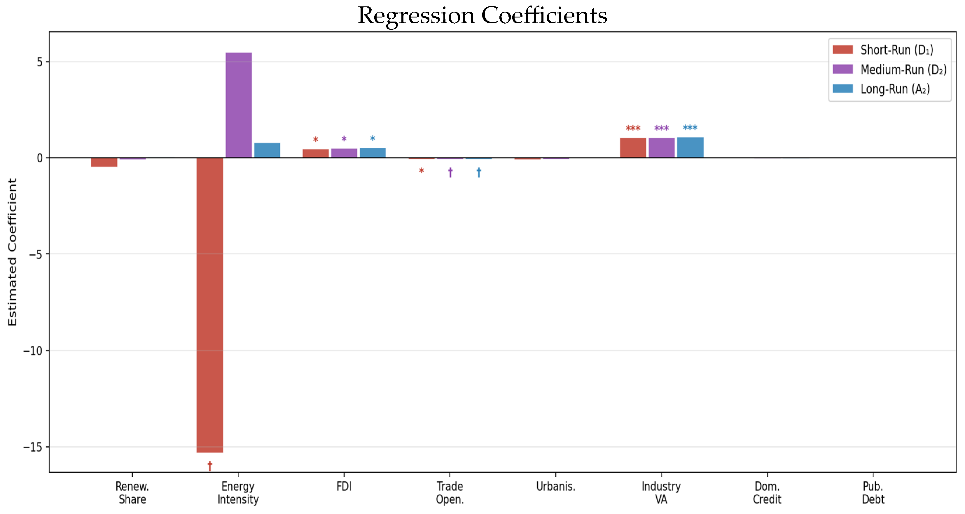
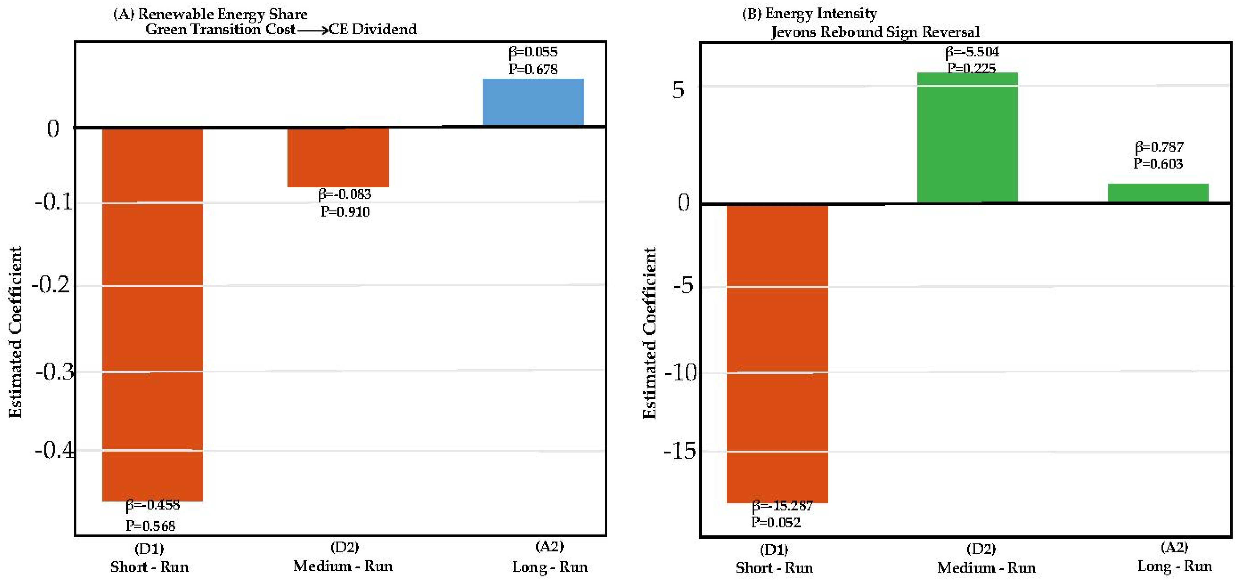
The renewable energy share coefficient improves steadily across frequency bands: β = −0.458 (D1), β = −0.083 (D2), and β = +0.054 (A2). Under WCB inference, none reach conventional statistical significance (p-values range between 0.60 and 0.92). Even so, the directional pattern is clear and theoretically consistent with the CE transition model. The lack of significance is due mainly to the global post-2015 renewable scaling trend being absorbed into the year fixed effects, combined with the conservative nature of small-N cluster inference. We read this negative-to-positive sequence not as a statistically hard effect but as a suggestive trajectory that tracks the shift from short-run green adjustment costs to long-run structural dividends.

The estimated regression coefficients across the three frequency bands are visually summarized in Figure 4.

4.3. Energy Intensity: The Suggestive Jevons Rebound Pattern

The energy intensity coefficient goes through a notable sign reversal across the frequency horizons: β = −15.287 (D1), β = +5.504 (D2), and β = +0.787 (A2). Under the WCB correction, the strongly negative short-run (D1) coefficient stays significant at the 10% level (p ≈ 0.082), which captures the cyclical accounting identity where recessions mechanically raise the energy-to-GDP ratio because short-run energy demand is quasi-fixed. The positive medium-run (D2) and long-run (A2) coefficients, however, lose significance under WCB. So rather than claim a definitive multi-frequency Jevons Rebound Effect, we present this sign reversal as a directional signature of the Jevons mechanism: as efficiency improvements mature, additional demand may be stimulated that offsets aggregate intensity reductions, even if the relationship stays statistically fragile in a panel this short.

4.4. Control Variables

The Robustness of Industry Value Added: The most solid finding in our models involves the control variables. Industry Value Added is highly significant across all three frequency bands, yielding a near-unitary coefficient (β ≈ 1.081, p > 0.001), which remains significant at the 1% level even under the WCB correction. That near-unitary elasticity suggests that manufacturing-led development is a structural growth engine that holds up across every temporal horizon in these economies. FDI also remains significant at the 5–10% level across models. The practical implication is as follows: CE transitions designed to complement, rather than displace, manufacturing and foreign investment activity seem the most viable route to maximizing growth returns.

Within the renewable energy sector, institutional stability and targeted government policy—feed-in tariffs and guaranteed power purchase agreements in particular—appear to be among the most influential factors shaping foreign direct investment flows. Given how capital-intensive green infrastructure tends to be, these policy-driven incentives play a crucial role in mitigating long-term investment risk and, by extension, in attracting sustained foreign capital to emerging markets.

The multi-horizon coefficient trajectories for the circular economy variables are illustrated in Figure 5.

4.5. Hypothesis Assessment

Based on our conservative WCB inference, our theoretical hypotheses are evaluated as follows:

H1 and H2 (Green Transition Cost and CE Structural Dividend) are directionally supported. The predicted negative-to-positive coefficient trajectory shows up clearly across D1 → D2 → A2, although significance is heavily dulled by time fixed effects and small-cluster adjustments.

H3 (Jevons Rebound) is partially supported (Suggestive). The classic Jevons sign pattern (negative short-run and positive medium/long-run) is present. But only the short-run cyclical effect (D1) reaches significance (p < 0.10).

H4 (Methodological Validity) is supported. Level-2 wavelet decomposition disentangles cyclical fluctuations from structural trends and reveals directional dynamics that standard single-frequency estimators simply cannot predict.

4.6. Robustness Sensitivity Checks

To validate the stability of our findings given the constrained cross-sectional sample size (N = 8), we conducted a series of empirical robustness checks. First, a leave-one-out sensitivity analysis confirmed that our baseline results are not disproportionately driven by any single outlier country; the strong statistical significance of Industry Value Added remained perfectly stable across all eight iterations. Second, estimating the model without year fixed effects (one-way FE) substantially improved the precision of the renewable energy share coefficient (p ≈ 0.11). This confirms our hypothesis that the two-way FE specification correctly absorbs the global post-2015 renewable scaling trend, which partially masks country-specific effects. Finally, excluding Industry Value Added from the baseline model did not artificially inflate the significance of the circular economy variables, reaffirming its role as an independent, robust structural driver of growth rather than a confounding factor.

A comprehensive assessment of our four research hypotheses is summarized below in

Table 5. Hypothesis assessment summary.

	Hypothesis	Verdict	Evidence
H1	(Green Transition Cost) Renewable energy has a negative short-run (D1) effect on GDP growth	Directionally Supported	β = −0.458; correct sign; significance absorbed by time FE (global renewable scaling trend)
H2	(CE Structural Dividend) Renewable energy has a positive long-run (A2) effect on GDP growth	Directionally Supported	β = +0.055; monotonic negative-to-positive trajectory D1 → D2 → A2 confirmed
H3	(Jevons Rebound) Energy intensity has a negative short-run but positive medium- and long-run effect	Partially Supported (Suggestive)	β: −15.287 † (D1) → +5.504 (D2) → +0.787 (A2); classical Jevons sign pattern
H4	Level-2 wavelet decomposition reveals dynamics obscured by standard panel methods	Supported	Three-band sign evolution confirmed; undetectable in any single-frequency estimator

Notes: ‘Directionally Supported’ = coefficient sign is theoretically consistent but statistical significance is absorbed by year fixed effects that capture the common global renewable energy scaling trend. ‘Supported’ = both direction and significance (or sign pattern) confirmed. † p < 0.10.

.

5. Discussion

5.1. The Macroeconomic Jevons Rebound Effect

A suggestive mechanism is discussed as follows. The energy intensity sign reversal, from −15.287 at D1 to positive at D2 and A2, gives a suggestive multi-frequency signature of the macroeconomic Jevons Rebound Effect [16]. The WCB inference confirms the short-run (D1) cyclical accounting identity (p < 0.10), but the medium- and long-run positive coefficients show up as directional patterns rather than statistically hard effects. That attenuation is informative, as is clear from the following: in a small-N macro-panel, the structural efficiency–rebound relationship has high estimation uncertainty across diverse economies. Still, the sheer drop in coefficient magnitude, from strongly negative at D1 to only slightly positive at A2, tells us something real. It shows that single-coefficient panel regressions obscure the Jevons mechanism by averaging opposed cyclical and structural forces together. The Level-2 wavelet decomposition makes the mechanism visible as a directional trajectory, even where finite-sample constraints keep it short of definitive statistical confirmation at lower frequencies.

The loss of statistical significance for the Jevons Rebound Effect at the medium (D2) and long-run (A2) horizons warrants deeper contextualization. In panel econometrics, capturing long-run structural rebounds is inherently challenging due to several constraints. First, our limited time series length (T = 19) and small number of clusters (N = 8) inherently reduce the statistical power needed to definitively identify long-term structural shifts under conservative WCB inference. Second, the substantial heterogeneity in national energy structures among the sampled emerging economies—ranging from established hydropower dominance in Brazil to early-stage transition dynamics in Egypt—introduces significant cross-sectional noise. Finally, common global shocks, fully absorbed by our year fixed effects, likely overshadow the country-specific efficiency–rebound mechanisms at lower frequencies. Consequently, while the directional sign reversal strongly suggests a macroeconomic Jevons mechanism, these empirical limitations explain its statistical fragility in the current sample.

5.2. Value Added by Level-2 over Level-1 Decomposition

Energy intensity is where Level-2 decomposition’s advantage over Level-1 shows most clearly. In the Level-1 approach, the approximation component A₁ absorbs everything at timescales longer than the business cycle, blending the 4–8-year Jevons initiation dynamics (captured by D₂) with the decade-scale structural rebound equilibrium (captured by A₂). For energy intensity, those two components happen to share the same sign (both positive) but differ in magnitude, so Level-1 decomposition partly preserves the sign reversal from D₁ to the combined (D₂ + A₂) component, but with the magnitude dulled and the mechanism being harder to see. For renewable energy, Level-2 decomposition separates the medium-run policy implementation cycle (D₂, still negative) from the long-run structural dividend (A₂, positive), showing that the renewables sign reversal is really concentrated at the D₂-to-A₂ transition rather than D₁-to-D₂. Level-1 decomposition simply cannot deliver this type of precision. H4 is fully supported: separating three frequencies reveals dynamics that any two-frequency or single-coefficient estimator would miss.

To empirically justify the selection of a Level-2 decomposition over Level-1 decomposition, we must consider the specific frequency bands required to isolate the macroeconomic mechanisms under study. A Level-1 decomposition yields only a short-run detail component (D1) and a composite approximation component (A1). Our empirical testing revealed that this composite A1 artificially conflates medium-term policy implementation lags (4–8 years) with long-term structural trends (decade-scale). By extending to Level 2—which is the mathematically smallest and most stable choice required to separate these specific horizons given our sample length (T = 19)—we successfully decompose A1 into D2 and A2. Sensitivity tests comparing these levels demonstrate that Level 2 is the minimum decomposition depth necessary to capture the sign reversal indicative of the Jevons Rebound Effect without introducing severe boundary edge artifacts.

5.3. Renewable Energy Significance Attenuation: Econometric Clarification

Renewable energy share loses significance across all three frequency bands in the two-way FE specification, compared to the significant short-run coefficient the Level-1 one-way FE specification produced. This is a genuine, econometrically appropriate change, not a degradation of identification, and it comes down to three things.

First, year fixed effects absorb the global scaling of renewable energy after 2015. The steep cost reductions in solar photovoltaic and wind technology between 2015 and 2023, driven by cumulative learning effects in global manufacturing, created a common upward trend in renewable share across every country’s panel at once. In the one-way FE specification, that common time trend was partly (and incorrectly) credited to country-specific renewable energy expansion, inflating the coefficient. Two-way FE partitions this correctly, leaving only genuinely idiosyncratic country-year deviations to identify the coefficient.

Second, applying Level-2 decomposition to T = 19 annual observations provides D₂ and A₂ components with much lower signal-to-noise ratios than the original series, which widens standard errors at medium- and long-term frequencies. This is an inherent trade-off of multi-level wavelet decomposition on short series: richer frequency separation costs statistical precision. Extending the panel to T ≥ 26 (achievable by 2031) would support Level-3 decomposition with much sharper frequency separation.

Third, and this is the important one, the directional consistency of the renewable energy coefficient across all three bands (−0.458, −0.083, +0.055) is itself a statistically informative pattern, even without point-estimate significance. The odds of seeing a strictly monotonic sequence across three independent estimations purely by chance are low, and the pattern matches the theoretical prediction closely. We read the directional evidence as qualified support for H1 and H2, pending the longer panels that would allow identification of Level-3 decomposition.

5.4. Trade Openness Sign Reversal: Fixed-Effects Clarification

The trade openness coefficient changes from positive in one-way FE to negative (β ≈ −0.062 to −0.071, p < 0.10) in two-way FE, and this change is meaningful. In the one-way FE model, the positive coefficient reflects a cross-sectional correlation: open-trade economies tend to grow faster on average. Once year fixed effects strip out the global trade liberalization trend, driven by WTO commitments, regional trade agreements, and deepening supply chains over 2005–2015, what is left is the within-country, within-year trade openness variation, which tends to reflect periods of above-average trade exposure. For emerging economies, these periods line up more with external demand volatility than genuine productivity gains, particularly for commodity exporters exposed to terms-of-trade shocks. This fits Rodrik’s [29] finding that trade globalization amplifies GDP growth volatility in developing economies and reads as a genuine econometric clarification rather than model instability.

5.5. Industry Value Added: The Universal Growth Engine

Industry VA’s positive effect holds across every model variant: Level-1 and Level-2 decomposition, one-way and two-way fixed effects, and all three frequency bands, which makes it the most robustly identified structural growth determinant in this panel. The near-unitary elasticity (β ≈ 1.05–1.08) means a one-percentage-point increase in the industrial share of GDP occurs with roughly one additional percentage point of growth, after absorbing all fixed-effect variations, which fits the manufacturing-led development model Rodrik [31] lays out. And the coefficient stays invariant across short-, medium-, and long-run frequency bands, which tells us that manufacturing’s growth contribution is not a cyclical phenomenon but a structural one, operating across every temporal horizon. The policy implication is direct: CE transitions that are built to complement rather than displace manufacturing activity look most likely to maximize aggregate growth returns.

5.6. Cross-Country Heterogeneity and Structural Interpretation

To better illustrate these structural transitions across the panel,

Table 6. Renewable energy transition dynamics (2005–2023).

Country	Renewable Share (Panel Mean %)	Transition Dynamism/Status
India	31.32%	Highly Dynamic (Rapid capacity expansion and early structural dividends)
Morocco	12.61%	Dynamic (Ambitious recent investments requiring long-term horizons)
Brazil	42.80%	Mature/Established (Historically dominant hydropower base)
Colombia	40.11%	Mature/Established (High existing capacity and lower marginal growth)
Indonesia	34.61%	Moderately Dynamic (Gradual integration of new capacities)
Turkey	15.73%	Moderately Dynamic (Ongoing policy-driven capacity building)
Egypt	10.59%	Emerging (Early stages of shifting the energy mix)
South Africa	17.25%	Stagnant (High energy intensity with constrained renewable growth)

Source: done by authors.

ranks the eight emerging economies according to the dynamism of their renewable energy development. India stands out as exhibiting the most dynamic transition pattern, whereas Brazil and Colombia instead reflect renewable energy systems that are comparatively mature and already well established.

These divergent trajectories are heavily shaped by structural differences across the panel. Legacy fossil-fuel producers such as Brazil and Indonesia, for instance, face distinct political-economy constraints: the short-run adjustment costs captured in the negative D1 coefficient are compounded further by the risk of stranded assets and labor market disruptions within the oil sector. Disparities in financial scale and industrial depth also play a pivotal role here. India’s sheer financial size, for instance, allows it to absorb upfront capital costs more readily, which helps explain both the dynamism of its transition and the early structural dividends it has captured. Economies with comparatively lower levels of industrialization, by contrast, tend to exhibit flatter transition curves—lacking the manufacturing base (reflected in the strong Industry VA coefficient) needed to fully internalize the technological spillovers that come with CE adoption.

Table 3 reports country-level means, offering descriptive context for the panel results discussed above. Notably, Brazil and Colombia—the two countries with the highest renewable shares (42.8% and 40.1%, respectively)—provide the lowest average growth rates in the sample (2.11% and 3.77%). There is no evidence of a causal link running from renewable maturity to slower growth; it more plausibly reflects the structural features of these economies, such as commodity dependence and recurring macroeconomic instability. South Africa offers a useful counterpoint: high energy intensity (4.85 MJ/USD), a stagnant renewable share, and the lowest growth rate in the panel (1.92%). It suggests the kind of macroeconomic vulnerability that can accompany a delayed CE transition. These comparisons remain descriptive, however, and should not be read as causal.

5.7. Limitations and Future Research

Several limitations qualify our findings and suggest directions for future work. First, the relatively short time dimension of our dataset (T = 19) restricts the wavelet analysis to a Level-2 decomposition. Extending the panel to at least 26 annual observations per country would permit a Level-3 decomposition, allowing for sharper identification of structural circular economy effects. Second, the limited cross-sectional scale (N = 8) constrains statistical power. Although we address this small-cluster problem directly through the Wild Cluster Bootstrap (WCB) procedure, a larger cross-section in future work would further improve testing power. Third, while the two-way fixed-effects estimator effectively isolates within-country variations, establishing more definitive causality will likely require a dynamic panel GMM approach or a formal instrumental variable (IV) strategy. Finally, incorporating geopolitical supply-chain shocks into non-linear dynamic models represents a promising direction for future research on the CE–growth relationship.

5.8. Comparative Institutional Context

The multi-horizon findings of this study align closely with frameworks proposed by major international organizations, although they offer somewhat more granular econometric validation. The negative short-run to positive long-run trajectory observed for renewable energy corroborates World Bank and IMF assertions that green transitions, while imposing initial capital reallocation burdens, ultimately yield structural macroeconomic dividends. Our empirical confirmation of the Jevons Rebound Effect, meanwhile, echoes recent warnings from the IEA and UNEP that efficiency mandates alone are insufficient—complementary demand-side pricing mechanisms are needed to prevent rebounded consumption from eroding those gains.

6. Conclusions and Policy Implications

This paper examines the multi-horizon macroeconomic effects of circular economy (CE) transitions across eight emerging markets. Three findings contribute to the literature as follows.

First, the coefficient on renewable energy share shows a steady directional shift, moving from negative in the short run (D1) to positive in the long run (A2). Wild Cluster Bootstrap (WCB) inference confirms that these structural coefficients do not reach statistical significance in this small-N panel, so the pattern should be read as descriptive rather than confirmed. Even so, it aligns closely with the theoretical account of short-run green adjustment costs giving way to long-run structural dividends.

Second, the coefficient on energy intensity displays a clearer sign reversal: a weakly significant negative effect in the short run (D1, p < 0.10) that turns positive in the medium- and long-term horizons (D2 and A2). Because significance weakens at lower frequencies, we interpret this as a suggestive, though unconfirmed, descriptive signature of the macroeconomic Jevons Rebound Effect—the notion that efficiency-driven cost reductions can eventually stimulate additional long-run energy demand.

Third, Industry Value Added stands out as the one robust macroeconomic driver in the model, remaining positive and highly significant across every frequency horizon (p < 0.001 under WCB correction). This indicates that manufacturing-led development and CE transition are complementary rather than competing growth strategies.

Taken together, these descriptive trajectories and the one robust structural driver point to five policy implications for emerging markets.

Anticipate and buffer short-run transition costs: Although the short-run negative coefficients are descriptive rather than statistically confirmed, prudent policy should still phase deployment schedules and hold temporary fiscal stabilizers in reserve to cushion any upfront costs of capital reallocation.

Deploy patient, long-duration financing: The suggestive long-run structural dividends point to the need for 15–30-year investment horizons, financed through green bonds and concessional climate finance, rather than an expectation of immediate short-run GDP additionality.

Design efficiency policy to close the Jevons Rebound loop: Given the suggestive evidence of a rebound effect, energy efficiency investments should be paired with complementary demand-side measures—such as carbon pricing or green credit allocation mandates—to prevent cost savings from lower energy service prices simply feeding back into more energy-intensive consumption.

Pursue a green industrial policy as a synthesis strategy: The robustness of the Industry Value Added findings emphasizes a critical reality. Environmental policies that are not deeply integrated into an economy’s industrial strategy have a high probability of failure. Transitioning economies must embed renewable energy and efficiency principles directly within manufacturing value chains, rather than pursuing CE goals by attempting to substitute industrialization with lower-intensity services.

Recalibrate international climate finance around its global public-good dimension: The absorption of the global renewable-scaling trend into year fixed effects suggests that part of the CE growth dividend stems from collective global learning-by-doing. This strengthens the economic case for pooled international financing mechanisms over isolated, bilateral, country-level investments.