Article

Development of an Inexact Regional Aquaculture System Planning Model to Provide Corresponding Optimal Sustainable Resource Allocation Schemes

1
Xiamen Key Laboratory of Intelligent Fishery, Xiamen Ocean Vocational College, Xiamen 361102, China
2
School of Environmental Science and Engineering, Xiamen University of Technology, Xiamen 361024, China
3
School of Film Television and Communication, Xiamen University of Technology, Xiamen 361024, China
*
Author to whom correspondence should be addressed.
Sustainability 2026, 18(17), 8761; https://doi.org/10.3390/su18178761
Submission received: 7 June 2026 / Revised: 6 August 2026 / Accepted: 10 August 2026 / Published: 26 August 2026

Abstract

The Guidelines for Sustainable Aquaculture (GSAs) emphasize that formulating proper regional development plans is essential for achieving sustainable growth in aquaculture. Conventional research has limitations in allocating resources from a regional scale, subject to various constraints relating to the social, economic, environmental, and other domains. To fill this research gap, this study proposes an inexact regional aquaculture system planning model (IRAM) to optimally allocate resources including energy, water, area, media, and labor among various aquaculture species across multiple aquafarms under uncertainty. The model is applied to Fujian Province, China, over a 15-year planning horizon (2026–2040, three 5-year periods). As model-based scenario insights derived under specific assumptions, the main findings are as follows: (i) the system cost would increase by [18.75, 20.00]%, while the product output would greatly rise by [41.57, 47.54]% from period 1 to period 3; (ii) renewable energy (wind and solar) would supply [60.32, 81.05]% of the total electricity by period 3; (iii) shallow-sea culture ([48.6, 50.2]%) and pond culture ([17.6, 18.8]%) would receive the highest media allocation via internet platforms, supporting community communication; and (iv) pollutant and carbon emissions would decline due to the adoption of low-carbon feed and renewable energy penetration. The findings are scenario-dependent, and their practical applicability relies on the sensitivity analysis and model code/data availability discussed in the main text. One limitation lies in its inadequate ability to handle stochastic and fuzzy information commonly encountered in real-world planning problems.

1. Introduction

Fishery is a crucial sub-industry belonging to agriculture, which provides nutritious aquatic food to support the healthy life of human beings. For the purpose of satisfying the huge aquatic food demand and protecting good aquatic ecological environments, aquaculture has exceeded capture fisheries to become the major measure in obtaining aquatic food. For example, globally, aquaculture provided 51% of aquatic products in 2022 [1,2]. According to the Guidelines for Sustainable Aquaculture (GSAs), it is necessary to formulate proper regional development plans for sustainable aquaculture growth [3]. A typical aquaculture system should support the growth of aquatic species (from seed to maturity) with enough resources, such as water, energy (e.g., electricity), feed, space, labor, medicine, etc. In the growth process, many problems often hinder the sustainable development of aquaculture systems, including discharging nutrient pollutants (e.g., nitrogen and phosphorus), emitting greenhouse gases (e.g., carbon dioxide and methane), wasting natural resources (e.g., water, land, and energy), lacking social responsibility (e.g., low wages and gender discrimination), not being accepted by local communities, etc. [4,5]. How to make regional sustainable aquaculture resource allocation plans after considering the interactions among these problems concerns decision-makers. System optimization models, formulated based on objective functions and constraints, can effectively generate optimal quantitative plans [6]. To build the models, system boundaries and components should be firstly recognized; components’ relationships should then be quantified; and, finally, objective functions (e.g., minimizing aquaculture cost, and maximizing aquaculture products) and constraints (allowed negative impacts to society, the environment, the economy, ecology, etc.) should be determined [7].
Researchers have constructed system optimization models to manage aquaculture farms with different objective functions and constraints, and plans related to aquaculture products, feeding alternatives, energy mixes, water utilization, and so on have been obtained [8,9,10]. Luna et al. provided the optimal operation plans for a fish farm, including the economic factors, environmental concerns, and product quality. New types of model constraints, such as labor and market capacities for maximizing the weekly harvested fish volume, were found [11]. Nguyen et al. designed a model to minimize aquaculture farms’ hybrid energy cost with the constraints of the supply–demand balance, capacity expansion limitation, carbon emission allowance, etc.; the results of a shrimp farm operation case showed an obvious reduction in energy cost and carbon emission [12]. Li et al. proposed a model to maximize a fish farm’s product weight in the face of constraints, including feed demands and growth features; it was found that the fish product weight would increase by 36.36% compared with conventional feeding methods [13]. Liu et al. built a model to provide optimal water and electricity allocation plans for an aquaculture farm with a minimized cost subjected to the constraints of requirement supply, capacity boundaries, etc. It was found that the model could reduce the power grid’s load and operation costs through a case study [14]. Zhang et al. developed a model to minimize a fish farm’s annualized energy cost in the face of constraints related to demand supply, healthy growth, carbon reduction, etc. It was found that the cost of the studied system could decrease by 35% [15]. Dolatabadi and Ricardez-Sandoval proposed a model to maximize the fish farm systems’ annual profit with constraints of stocking density, market demand, oxygen level, and nitrogen discharge; the results showed an increment in the profit of the studied farm after optimization [16]. These studies have proposed basic frameworks for system optimization models to provide aquaculture resource allocation plans. However, they only plan for individual or several farms and consider limited constraints. The above models are not suitable to provide plans which cover large-scale areas, long-term periods, and various restrictions.
It is worth noting that numerous regional system optimization models, which aimed to allocate resources sustainably, were developed and applied in the field of other sub-industries (e.g., crop farming and livestock husbandry) of agriculture [17,18,19]. Li et al. developed a water–land allocation model to decide different crops’ land area and water volume in a large irrigation district in Northeast China; optimal plans after balancing perspectives of economic benefit, resource equity, and carbon emissions were obtained [20]. Ren et al. proposed a water–energy–land allocation model to detect the land, electricity, and water allocation plans of diverse crops in the Yellow River Basin (in China); optimal plans which could lead to an increased water productivity, reduced carbon emissions, and enhanced regional competitiveness were gained [21]. Yuan et al. developed a water–land–food allocation model to optimally allocate water and land for various crops to maximize the irrigation productivity of a district in the Yellow River Basin, where constraints of water demand, land availability, and food security were considered [22]. Li et al. developed a water allocation model for various crops in the Tarim River Basin (in China); plans—after balancing the conflicts among water scarcity, economic benefit, carbon emissions, and pollutant discharge—were generated [23]. Feng et al. presented a water–energy–food allocation model to determine the water volume, crop area, and livestock population in Sichuan Province (in China); allocation plans after handling conflicts among economic benefit, resource inequity, production efficiency, and carbon emission were obtained [24]. These models generated the optimal amounts of water, electricity, and/or land allocated to various crops in a region during a certain period, and the results showed they were useful. Few scholars conducted such research to support sustainable aquaculture development. Meanwhile, uncertainty often exists in the decision-making processes due to the natural, political, social, and economic factors’ variations. Suitable uncertain analysis methods, such as stochastic, interval, and fuzzy methods, can be adopted to help control the risk of decision failure [25]. Among them, interval methods handle the problem in which variables are expressed as interval values rather than precise values. They have been integrated into a variety of regional resource allocation models [26,27,28].
While numerous regional optimization models have been developed for crop farming and livestock husbandry, these models are not directly applicable to aquaculture systems. The major differences are as follows: (1) aquaculture species exhibit distinct biological growth patterns and survival rates; (2) aquaculture relies on both freshwater and seawater resources; (3) aquaculture involves specific feed conversion ratios, medicine usage, and pollutant discharge; (4) aquaculture planning requires the consideration of social factors such as labor gender structure, community acceptability, and reputation improvement, which are rarely integrated in existing water–land–food and water–energy–food allocation models. No regional-scale optimization model has been developed to handle these aquaculture-specific challenges.
To fill this gap, the proposed IRAM offers three levels of innovation: (1) Methodologically, it incorporates an interval programming approach to cope with parametric uncertainties, generating flexible interval solutions rather than single-point estimates; mathematical equations and inequalities are adopted to quantify the component interactions and establish standardized objective functions and constraint conditions once the studied system is identified. (2) System-boundary, it is the first model to simultaneously integrate product (e.g., fish, shrimp–crab, shellfish, and algae), energy (e.g., wind, sun, diesel, and others), water (e.g., surface water, groundwater, and seawater), labor (e.g., male and female), space (e.g., inland area and sea area), feed (e.g., conventional and low-carbon), medicine, emissions, and communication constraints within a single aquaculture planning framework. (3) Application, it is the first model applied to Fujian Province at the regional scale, covering various farm types and species over a 15-year horizon; the solutions include optimal seed input, product output, energy capacity expansion, water allocation, labor structure, feed and medicine consumption, and media episode distribution, which provide technical support for decision-makers to formulate aquaculture plans.

2. Materials and Methods

2.1. System Boundary Definition

The IRAM is defined by four interconnected boundaries that specify the scope and assumptions of the model:
(1)
Spatial boundary: The primary decision unit is the administrative region of Fujian Province, with aquaculture production disaggregated by nine aquaculture area types (MRC, MUC, OSC, POC, REC, STC, LAC, PAC, and OFC) and four species (fish, shrimp–crab, shellfish, and algae). The model aggregates production at the regional scale and does not represent single farm-level operations.
(2)
Temporal boundary: The planning horizon covers 15 years (2026–2040), divided into three 5-year periods aligned with China’s national five-year planning cycles (Pe1 for 2026–2030; Pe2 for 2031–2035; and Pe3 for 2036–2040). All decision variables and constraints are time-dependent.
(3)
Technological boundary: The model incorporates three aquaculture production modes: extensive (EXM), semi-intensive (SIM), and intensive (INM), which are distinguished by input intensity and facility requirements. Regarding energy supply, it includes four technologies, wind power, solar power, diesel power, and grid power, with capacity expansion and storage options for renewables.
(4)
Management boundary: The model is established from the perspective of regional decision-makers who seek to minimize total system costs subject to multi-dimensional sustainability constraints. Decision variables include seed input, energy mix, water allocation, labor employment, feed and medicine consumption, and media output. External parameters include resource availability, market demand, unit costs, emission coefficients, and technology performance factors.

2.2. System Operation Description

The aquaculture system studied in this paper is conceptualized as a two-layer hierarchical framework (Figure 1): aquaculture system construction and optimization model formulation. This structure facilitates a clear understanding of how the IRAM transforms resource inputs into sustainable allocation schemes.

2.2.1. Aquaculture System

The system encompasses three aquaculture production modes, classified by stocking density, facility intensity, and management level:
(a)
Extensive mode (EXM): This mode features aquaculture zones with minimal or no facilities, relying primarily on natural resources (e.g., tidal exchange and natural feed). The office zone operates at a low management level. This mode is characterized by low investment cost, low product output per unit area, and high environmental risk due to limited pollution control.
(b)
Semi-intensive mode (SIM): This mode builds upon EXM by adding facilities such as feeders, monitors, aerators, lights, and thermostats in the aquaculture zone. The office zone is upgraded to a medium management level, and a resources zone with medium renewable energy capacity is incorporated. This mode offers moderate investment cost, product output, and environmental risk.
(c)
Intensive mode (INM): This mode further upgrades the aquaculture zone with smarter facilities, such as automated feeding, real-time water quality sensors, recirculating systems. The office zone and renewable energy level are both elevated to high standards. INM is characterized by high investment cost and high product output. Some INM farms are equipped with tailwater treatment facilities that achieve high water recycling efficiency, while others discharge untreated tailwater directly, posing significant environmental risks.
The system purchases seeds of four species groups (including fish, shrimp–crab, shellfish, and algae), and cultivates them across nine aquaculture area types: shallow-sea culture (MRC), tidal-flat culture (MUC), offshore culture (OSC), pond culture (POC), reservoir culture (REC), stream culture (STC), lake culture (LAC), paddy culture (PAC), and other freshwater culture (OFC). The three modes, which constitute the core framework of the system (Supplementary Material Table S1 shows the comparisons among them), together with the nine aquaculture area types, require various resources, including energy, water, labor, land/sea space, feed, medicine, and media, all of which are quantified as decision variables in the optimization module.

2.2.2. Optimization Model

The core of the IRAM is an interval linear programming model that converts the physical system description into a mathematically tractable optimization problem. The model is formulated with the following components:
Objective function: Minimize the total system costs;
Resource availability constraints: Constraints on energy supply, water availability, land/sea area, and labor capacity;
Demand–supply balance constraints: Constraints ensuring that product output satisfies market demand, seed input meets production targets, and feed/medicine consumption supports healthy growth;
Environmental limit constraints: Constraints capping pollutant discharges (TN, TP, SS, and COD), direct and indirect carbon emissions, and tailwater quality parameters to comply with official regulatory standards;
Social responsibility constraints: Constraints mandating minimum wage standards, female labor participation ratios, and community communication efforts via media output;
Uncertainty handling: All parameters are expressed as intervals to reflect the inherent uncertainties in data sources and future projections.
The optimal solutions generated by the IRAM are interpreted as policy-relevant parameters across three sustainability dimensions:
Economic decisions: Total system costs, product output by species and area type, feed and medicine consumption, and infrastructure investment requirements;
Environmental decisions: Pollutant discharges (TN, TP, SS, and COD), carbon emissions and sequestration (including shellfish–algae carbon sink), renewable energy penetration rates, and water consumption by different sources;
Social decisions: Employment structure (gender-based labor distribution), media episode allocation by farm types and communication platforms, and community acceptability proxy measures.
These decisions provide decision-makers with actionable allocation schemes regarding energy capacity expansion, water diversion, labor deployment, feed and medicine regulation, and public communication strategies. All results are presented as interval ranges to accommodate parameter uncertainty, and their scenario-dependent nature is emphasized in the discussion.

2.3. Inexact System Planning Model Formulation

It is assumed that decision-makers require cost-effective schemes; thus, the model’s objective function is to minimize the total system costs ( f ± ), which comprises the costs of purchasing seed ( f 1 ± ), the costs of using water ( f 2 ± ), the costs of purchasing bait and medicine ( f 3 ± ), the costs of paying wage ( f 4 ± ), the costs of treating sewage ( f 5 ± ), the costs of consuming energy ( f 6 ± ), the costs of constructing infrastructure ( f 7 ± ), the costs of mitigating carbon ( f 8 ± ), and the costs of producing videos or image-text ( f 9 ± ). The objective function is listed as follows (Appendix A is the parameter list):
f ± = f 1 ± + f 2 ± + f 3 ± + f 4 ± + f 5 ± + f 6 ± + f 7 ± + f 8 ± + f 9 ±
with
f 1 ± = a = 1 A k = 1 K t = 1 T ( N F E a , k , t ± + N F S a , k , t ± + N F I a , k , t ± ) U C F a , k , t ±
f 2 ± = a = 1 A k = 1 K t = 1 T A S W a , k , t ± C S W a , k , t ± + a = 1 A k = 1 K t = 1 T A G W a , k , t ± C G W a , k , t ±   + a = 1 A k = 1 K t = 1 T A S E a , k , t ± C S E a , k , t ±
f 3 ± = a = 1 A k = 1 K i = 1 I ( T C F a , k , t ± U O F a , k , t ± + T L F a , k , t ± U L F a , k , t ± + T L M a , k , t ± U L M a , k , t ± )
f 4 ± = a = 1 A k = 1 K t = 1 T L A F a , k , t ± U I C a , k , t ± + a = 1 A k = 1 K t = 1 T L A M a , k , t ± U I C a , k , t ±
f 5 ± = a = 1 A k = 1 K t = 1 T N F I a , k , t ± U W T a , k , t ± x r a , k , t ± L t / I D I a , k , t ±
f 6 ± = a = 1 A k = 1 K t = 1 T E W T a , k , t ± W E S a , k , t ± + a = 1 A k = 1 K t = 1 T E P P a , k , t ± B E S a , k , t ±   + a = 1 A k = 1 K t = 1 T E D G a , k , t ± D S E a , k , t ± + a = 1 A k = 1 K t = 1 T E P G a , k , t ± N P A a , k , t ±   a = 1 A k = 1 K t = 1 T S E W a , k , t ± B E E a , k , t ± a = 1 A k = 1 K t = 1 T S E P a , k , t ± B E P a , k , t ±   + a = 1 A k = 1 K t = 1 T ( E B E a , k , t ± I N B a , k , t ± + N W E a , k , t ± I N W a , k , t ± )   + a = 1 A k = 1 K t = 1 T E B P a , k , t ± I N P a , k , t ± + + a = 1 A k = 1 K t = 1 T P A E a , k , t ± I N E a , k , t ±   + a = 1 A k = 1 K t = 1 T E S P a , k , t ± I N S a , k , t ±
f 7 ± = a = 1 A k = 1 K t = 1 T ( N F E a , k , t ± N F E a , k , t 1 ± ) U C E a , k , t ± α k , t / ( I D E a , k , t ± H E I a , k , t ± )   + a = 1 A k = 1 K t = 1 T ( N F S a , k , t ± N F S a , k , t 1 ± ) U C S a , k , t ± β k , t ( 1 l e t ± ) / ( I D S a , k , t ± H E I a , k , t ± )   + a = 1 A k = 1 K t = 1 T ( N F I a , k , t ± N F I a , k , t 1 ± ) U C I a , k , t ± γ k , t ( 1 l e t ± ) / ( I D I a , k , t ± H E I a , k , t ± )
f 8 ± = a = 1 A k = 1 K t = 1 T E D G a , k , t ± P D E t ± / η t ± + a = 1 A k = 1 K t = 1 T E D G a , k , t ± C D E t ± P C E t ±   a = 1 A k = 1 K t = 1 T ( N F E a , k , t ± + N F S a , k , t ± + N F I a , k , t ± ) C O C a , k , t ± O C A a , k , t ±
f 9 ± = m = 1 M k = 1 K t = 1 T N M E m , k , t ± U M E t ± + k = 1 K t = 1 T N E P m = 1 , k , t ± U E P t ±   + k = 1 K t = 1 T N T V m = 2 , k , t ± U T V t ±
Constraints:
(1)
Aquaculture product: The number of surviving aquaculture species should be maintained at desired values. The surviving species should grow healthily, and the final weights of surviving aquaculture products should meet market demand. Specially, the average weights of aquaculture product are calculated based on the Von Bertalanffy Model [26].
a = 1 A N F E a , k , t ± / a = 1 A ( N F E a , k , t ± + N F S a , k , t ± + N F I a , k , t ± ) λ k , t ±
a = 1 A N F I a , k , t ± / a = 1 A ( N F E a , k , t ± + N F S a , k , t ± + N F I a , k , t ± ) λ k , t ±
k = 1 K ( N F E a , k , t ± + N F S a , k , t ± + N F I a , k , t ± ) N N S a , t ±
k = 1 K ( N F E a , k , t ± + N F S a , k , t ± + N F I a , k , t ± ) A N S a , t ±
I F D a , t ± k = 1 K ( N F E a , k , t ± S U F a , k , t ± + N F S a , k , t ± S U S a , k , t ± + N F I a , k , t ± S U I a , k , t ± ) ( W E L a , k , t ± w l a , k , t ± + W E M a , k , t ± w m a , k , t ± + W E H a , k , t ± w h a , k , t ± )
k = 1 K ( N F E a , k , t ± S U F a , k , t ± + N F S a , k , t ± S U S a , k , t ± + N F I a , k , t ± S U I a , k , t ± ) ( W E L a , k , t ± w l a , k , t ± + W E M a , k , t ± w m a , k , t ± + W E H a , k , t ± w h a , k , t ± ) A F D a . t ±
(2)
Energy consumption: For advanced aquaculture modes (e.g., semi-intensive and intensive modes), energy (i.e., electricity) is essential to support the operation of pumps, sensors, feeders, lights, aerators, thermostat (for heating to maintain water temperature), and/or other facilities (e.g., sewage treatment facilities) in aquaculture ponds, as well as daily labor activities. To fulfil energy consumption demand and promote green low-carbon development, wind power, solar power, diesel power, and grid power are selected as energy sources. The energy consumption should exceed the energy supply.
a = 1 A ( N F S a , k , t ± S U S a , k , t ± + N F I a , k , t ± S U I a , k , t ± ) ( W E L a , k , t ± w l a , k , t ± + W E M a , k , t ± w m a , k , t ± + W E H a , k , t ± w h a , k , t ± ) U E E a , k , t ± + a = 1 A N F I a , k , t ± L t x r a , k , t ± U E W a , k , t ± / I D I a , k , t ± + a = 1 A ( L A M a , k , t ± + L A M a , k , t ± ) U E L a , k , t ± a = 1 A ( E W T a , k , t ± + E P P a , k , t ± + E D G a , k , t ± + E P G a , k , t ± )
(3)
Energy availability: Sufficient diesel should be purchased to generate electricity through combusting.
a = 1 A k = 1 K E D G a , k , t ± / η t ± A D E t ±
(4)
Energy conversion: Wind energy, solar energy, and fossil energy (i.e., diesel) can be converted into electricity to fulfill the system’s energy requirement. The energy conversion abilities of wind turbines, photovoltaic panels, and diesel generators (depending on installed capacities and working hours) should be sufficient to generate enough electricity [27].
a = 1 A E D G a , k , t ± a = 1 A E B a , k , t ± T I C a , k , t ± ;   t = 1
a = 1 A E D G a , k , t ± a = 1 A ( E B a , k ± + t = 2 t E B E a , k , t ± ) ( 1 T E Y a , k , t ± ) T I C a , k , t ± ;   t 2
a = 1 A ( E W T a , k , t ± + S E W a , k , t ± ) a = 1 A N W a , k ± P W a , k , t ± T I W a , k , t ± + a = 1 A W B a , k ± W T a , k , t ± W D a , k , t ± ;   t = 1
a = 1 A ( E W T a , k , t ± + S E W a , k , t ± ) a = 1 A ( N W a , k ± + t = 2 t N W E a , k , t ± ) P W a , k , t ± ( 1 T W Y a , k , t ± ) T I W a , k , t ± + a = 1 A ( W B a , k ± + t = 2 t E B P a , k , t ± ) ( 1 T W S a , k , t ± ) W T a , k , t ± W D a , k , t ± ;   t 2
a = 1 A ( E P P a , k , t ± + S E P a , k , t ± ) a = 1 A P A a , k ± μ a , k , t ± G I a , k , t ± T I P a , k , t ± + a = 1 A P B a , k ± Y T a , k , t ± W P a , k , t ± ;   t = 1
a = 1 A ( E P P a , k , t ± + S E P a , k , t ± ) a = 1 A ( P A a , k ± + t = 2 t P A E a , k , t ± ) μ a , k , t ± G I a , k , t ± ( 1 T P Y a , k , t ± ) T I P a , k , t ± + a = 1 A ( P B a , k ± + t = 2 t E S P a , k , t ± ) ( 1 T P S a , k , t ± ) Y T a , k , t ± W P a , k , t ± ;   t 2
(5)
Renewable energy fraction: The electric power sector is one of the greatest carbon emission sources due to its heavy consumption of fossil energy (e.g., coal and natural gas). The system sets the ratios of wind electricity and solar electricity supply at specified values to help reduce the grid’s burden of pollutant and carbon emission mitigation.
a = 1 A k = 1 K ( E P P a , k , t ± + E W T a , k , t ± + S E W a , k , t ± + S E P a , k , t ± ) / a = 1 A k = 1 K ( E W T a , k , t ± + E P P a , k , t ± + E D G a , k , t ± + E P G a , k , t ± + S E W a , k , t ± + S E P a , k , t ± ) ς t ±
a = 1 A k = 1 K ( E P P a , k , t ± + E W T a , k , t ± + S E W a , k , t ± + S E P a , k , t ± ) / a = 1 A k = 1 K ( E W T a , k , t ± + E P P a , k , t ± + E D G a , k , t ± + E P G a , k , t ± + S E W a , k , t ± + S E P a , k , t ± ) σ t ±
(6)
Capacity expansion: The increment in aquaculture product demand may lead to increased electricity generation, and, thus, the installed capacity of each technology may need to be expanded. The expansion should consider construction ability and electricity demand.
a = 1 A ( N W a , k ± + t = 2 t N W E a , k , t ± ) P W a , k , t ± ( 1 T W Y a , k , t ± ) L M P k , t ±
a = 1 A ( N W a , k ± + t = 2 t N W E a , k , t ± ) P W a , k , t ± ( 1 T W Y a , k , t ± ) U W P k , t ±
a = 1 A ( P A a , k ± + t = 2 t P A E a , k , t ± ) μ a , k , t ± G I i , k , t ± ( 1 T P Y a , k , t ± ) L P P k , t ±
a = 1 A ( P A a , k ± + t = 2 t P A E a , k , t ± ) μ a , k , t ± G I i , k , t ± ( 1 T P Y a , k , t ± ) U P P k , t ±
a = 1 A ( E B a , k ± + t = 2 t E B E a , k , t ± ) ( 1 T E Y a , k , t ± ) L E B k , t ±
a = 1 A ( E B a , k ± + t = 2 t E B E a , k , t ± ) ( 1 T E Y a , k , t ± ) U E B k , t ±
(7)
Energy storage: Energy storage is crucial for wind and solar power supply, as it has the potential to enhance the stability of electricity supply in the aquaculture system [28].
a = 1 A ( W B a , k ± + t = 2 t E B P a , k , t ± ) ( 1 T W S a , k , t ± ) / a = 1 A ( N W a , k ± + t = 2 t N W E a , k , t ± ) P W a , k , t ± ( 1 T W Y a , k , t ± ) φ k , t min
a = 1 A ( W B a , k ± + t = 2 t E B P a , k , t ± ) ( 1 T W S a , k , t ± ) / a = 1 A ( N W a , k ± + t = 2 t N W E a , k , t ± ) P W a , k , t ± ( 1 T W Y a , k , t ± ) φ k , t max
a = 1 A ( P B a , k ± + t = 2 t E P P a , k , t ± ) ( 1 T P S a , k , t ± ) Y T a , k , t ± / a = 1 A ( P A a , k ± + t = 2 t P A E a , k , t ± ) μ a , k , t ± G I a , k , t ± ( 1 T P Y a , k , t ± ) ξ k , t min
a = 1 A ( P B a , k ± + t = 2 t E P P a , k , t ± ) ( 1 T P S a , k , t ± ) Y T a , k , t ± / a = 1 A ( P A a , k ± + t = 2 t P A E a , k , t ± ) μ a , k , t ± G I a , k , t ± ( 1 T P Y a , k , t ± ) ξ k , t max
(8)
Water utilization: Water is an important resource for aquaculture species’ survival and growth. Different aquaculture species require different types of water resources: freshwater for farming crayfish, grass carp, and other freshwater species; and seawater for farming lobster, large yellow croaker, and other marine species. Surface water and groundwater represent consumptive withdrawal, i.e., the volume of freshwater extracted from rivers, lakes, reservoirs, or aquifers for aquaculture use. This water is consumed during production via evaporation, seepage, and incorporation into biomass, and does not return to the source in a usable form. Freshwater aquaculture primarily relies on these sources, and the volume allocated to aquaculture should take into account competition with other sectors such as agriculture, industry, and domestic supply [29]. Seawater represents exchange or circulation volume rather than consumptive use. In marine aquaculture (e.g., shallow-sea culture, tidal-flat culture, and offshore culture), water is drawn from the sea, passes through the aquaculture system, and is returned to the sea. Only a small fraction is lost through evaporation or incorporated into products. For the purposes of this model, seawater quantities are treated as exchange volumes, not resource depletion. The area and water depth for marine aquaculture should be controlled to ensure environmental sustainability [30]. The water utilization should not be higher than the water supply, and the water supply should not be higher than the water availability.
a = 1 A [ ( N F E a , k , t ± ( 1 + h i a , k , t ± L t ) / I D E a , k , t ± ) + N F S a , k , t ± ( 1 + h s a , k , t ± L t ) / I D S a , k , t ± + N F I a , k , t ± ( 1 + h e a , k , t ± x r a , k , t ± L t ) / I D I a , k , t ± ] + a = 1 A ( E W T a , k , t ± + S E W a , k , t ± ) U W W a , k , t ± + a = 1 A ( E P P a , k , t ± + S E P a , k , t ± ) U W S a , k , t ± ( a = 1 A A S W a , k , t ± + a = 1 A A G W a , k , t ± ) ( 1 r l t ± ) + a = 1 A A S E a , k , t ± ; k , t
a = 1 A ( L A M a , k , t ± + L A F a , k , t ± ) U W A a , k , t ± ( a = 1 A A S W a , k , t ± + a = 1 A A G W a , k , t ± ) r l t ±
a = 1 A k = 1 K A S W a , k , t ± M S t ± A R W t ±
a = 1 A k = 1 K A G W a , k , t ± M G t ± A R W t ±
a = 1 A A S E a , k , t ± M S E k , t ±
(9)
Area usage: A typical aquaculture farm often contains an aquaculture zone, a sewage zone, a resources zone, and/or an office zone, depending on its aquaculture mode. The construction of wind turbines and photovoltaic panels also require land or water area. The area usage should not exceed the area demand, nor should it exceed the area availability.
( a = 1 a N F I a , k , t ± γ k , t / ( I D I a , k , t ± H E I a , k , t ± ) + a = 1 A N F S a , k , t ± β k , t / ( I D S a , k , t ± H E I a , k , t ± ) ) l e t ± a = 1 A ( N W a , k ± + t = 2 t N W E a , k , t ± ) ( 1 T W Y a , k , t ± ) U A W k , t ± + a = 1 A ( P A a , k , t ± + t = 2 t P A E a , k , t ± ) ( 1 T P Y a , k , t ± ) U A P k , t ±
a = 1 A N F E a , k , t ± α k , t / ( I D E a , k , t ± H E I a , k , t ± ) + a = 1 A N F S a , k , t ± β k , t / ( I D S a , k , t ± H E I a , k , t ± ) + a = 1 A N F I a , k , t ± γ k , t / ( I D I a , k , t ± H E I a , k , t ± ) A R E k , t ±
( a = 1 a N F I a , k , t ± γ k , t / ( I D I a , k , t ± H E I a , k , t ± ) + a = 1 A N F S a , k , t ± β k , t / ( I D S a , k , t ± H E I a , k , t ± ) ) l a t ± a = 1 A ( L A M a , k , t ± + L A F a , k , t ± ) U L O a , k , t ±
a = 1 A N F I a , k , t ± γ k , t ± l s t ± / ( I D I a , k , t ± H E I a , k , t ± ) a = 1 A N F I a , k , t ± x r a , k , t ± d x t / I D I a , k , t ±
(10)
Bait and medicine application: Bait provides various nutrients to support the growth of aquaculture species, and medicine ensures their health. Insufficient feeding may lead to the death of aquaculture species, and cannot obtain enough product output. Excessive feeding results in economic losses and water pollution; thus, the amounts of bait and medicine should be strictly controlled.
a = 1 A T C F a , k , t ± / a = 1 A ( T L F a , k , t ± + T C F a , k , t ± ) ω k , t ±
a = 1 A k = 1 K T L M a , k , t ± A L M t ±
( N F E a , k , t ± S U E a , k , t ± + N F S a , k , t ± S U S a , k , t ± + N F I a , k , t ± S U I a , k , t ± ) ( W E L a , k , t ± w l a , k , t ± U B L a , k , t ± + W E M a , k , t ± w m a , k , t ± U B M a , k , t ± + W E H a , k , t ± w h a , k , t ± U B H a , k , t ± ) T C F a , k , t ± + T L F a , k , t ±
( N F E a , k , t ± S U E a , k , t ± + N F S a , k , t ± S U S a , k , t ± + N F I a , k , t ± S U I a , k , t ± ) ( W E L a , k , t ± w l a , k , t ± U M L a , k , t ± + W E M a , k , t ± w m a , k , t ± U M M a , k , t ± + W E H a , k , t ± w h a , k , t ± U M H a , k , t ± ) T L M a , k , t ±
(11)
Social responsibility: To help eliminate gender discrimination and improve workers’ social status, these constraints ensure that the number of female laborers is maintained at a certain ratio and that all laborers’ wages are not below a minimum standard. Note: L A M a , k , t ± and L A F a , k , t ± are integer parameters.
a = 1 A k = 1 K L A F a , k , t ± W A F a , k , t ± + a = 1 A k = 1 K L A M a , k , t ± W A F a , k , t ± M W I t ±
a = 1 A k = 1 K L A F a , k , t ± W A F a , k , t ± + a = 1 A k = 1 K L A M a , k , t ± W A F a , k , t ± M W A t ±
a = 1 A N F I a , k , t ± F I L a , k , t ± ( 1 H Y F k , t ± ) + a = 1 A N F E a , k , t ± F E L a , k , t ± ( 1 H Y E k , t ± ) + a = 1 A N F S a , k , t ± F S L a , k , t ± ( 1 H Y S k , t ± ) a = 1 A L A M a , k , t ± + L A F a , k , t ±
a = 1 A k = 1 K L A F a , k , t ± / a = 1 A k = 1 K ( L A M a , k , t ± + L A F a , k , t ± ) ϑ t ±
(12)
Community acceptability: Community acceptability is defined as the degree of positive reaction following public assessments of alternative actions, attributes, or conditions. Common terms of community acceptability concerning aquaculture include concerns about eco-environment impacts, fair distribution of social-economic profits, competition for marine space, and integration with local culture to improve residents’ interests [31]. Since the former three themes are covered by other constraints, this constraint focuses on improving residents’ interests. Media is an effective tool for disseminating positive information about sustainable aquaculture development modes to the public. A proper number of high-quality videos and news items should be produced and uploaded.
m = 1 M N M E m , k , t ± M N M k , t ±
N M E m = 1 , k , t ± / m = 1 M N M E m , k , t ± R M E k , t ±
N E P m = 2 , k , t ± M E P k , t ±
N T V m = 1 , k , t ± M T V k , t ±
m = 1 M ( N M E m , k , t ± + N E P m , k , t ± + N T V m , k , t ± ) T M N k , t ± L G H k , t ±
L G H k , t ± = [ w 1 , k , t a = 1 A ( N F E a , k , t ± S U F a , k , t ± + N F S a , k , t ± S U S a , k , t ± + N F I a , k , t ± S U I a , k , t ± ) ( W E L a , k , t ± w l a , k , t ± + W E M a , k , t ± w m a , k , t ± + W E H a , k , t ± w h a , k , t ± )   / a = 1 A I F D a , k , t ± ] + [ w 6 , k , t ( a = 1 A E D G a , k , t ± C D E t ± + a = 1 A ( T L F a , k , t ± C L F t ± + T C F a , k , t ± C C F t ± ) ) / T C O k , t ± ] + ( w 2 , k , t T N E k , t ± / T N D k , t ± + w 3 , k , t T P E k , t ± / T P D k , t ± + w 4 , k , t T S E k , t ± / T S D k , t ± + w 5 , k , t T C E k , t ± / T C D k , t ± )
m = 1 M N M E m , k , t ± / m = 1 M ( N M E m , k , t ± + N E P m , k , t ± + N T V m , k , t ± ) R I M k , t ±
m = 1 M N T V m , k , t ± / a = 1 A ( N M E m , k , t ± + N E P m , k , t ± + N T V m , k , t ± ) R I T k , t ±
m = 1 M k = 1 K N M E m , k , t ± U M E t ± + k = 1 K N E P m = 2 , k , t ± U E P m = 2 , k , t ± + k = 1 K N T V m = 1 , k , t ± U T V m = 2 , k , t ± M X C t ±
(13)
Air quality: The pollutants and carbon emitted into the atmosphere mainly result directly from electricity generation (e.g., combusting diesel). They should be controlled to help mitigate climate change. It is worth noting that some aquaculture area types (e.g., algae mariculture) exhibit great carbon sequestration capacity, and can achieve negative carbon emissions.
a = 1 A k = 1 K E D G a , k , t ± N O t ± T N O t ±
a = 1 A k = 1 K E D G a , k , t ± P M t ± T P M t ±
a = 1 A k = 1 K E D G a , k , t ± S O t ± T S O t ±
a = 1 A E D G a , k , t ± C D E t ± + a = 1 A ( T L F a , k , t ± C L F t ± + T C F a , k , t ± C C F t ± ) T C O k , t ±
a = 1 A k = 1 K E D G a , k , t ± C D E t ± a = 1 A k = 1 K ( N F E a , k , t ± + N F S a , k , t ± + N F I a , k , t ± ) C O C a , k , t ± υ t ± T D C t ±
(14)
Water quality: Nitrogen, phosphorus, and suspended solids (originating from bait, medicine, excreta, sediment, etc.) in wastewater should be treated to improve water quality.
T N E k , t ± = { a = 1 A N F I a , k , t ± S U I a , k , t ± ( W E L a , k , t ± w l a , k , t ± U B L a , k , t ± + W E M a , k , t ± w m a , k , t ± U B M a , k , t ± + W E H a , k , t ± w h a , k , t ± U B H a , k , t ± ) c b n t ± + a = 1 A N F I a , k , t ± S U I a , k , t ± ( W E L a , k , t ± w l a , k , t ± U M L a , k , t ± + W E M a , k , t ± w m a , k , t ± U M M a , k , t ± + W E H a , k , t ± w h a , k , t ± U M H a , k , t ± ) c m n t ± + a = 1 A ( N F I a , k , t ± x r a , k , t ± L t o n t ± / I D I a , k , t ± ) } ( 1 r n a , k , t ± ) T N D k , t ±
T P E k , t ± = { a = 1 A N F I a , k , t ± S U I a , k , t ± ( W E L a , k , t ± w l a , k , t ± U B L a , k , t ± + W E M a , k , t ± w m a , k , t ± U B M a , k , t ± + W E H a , k , t ± w h a , k , t ± U B H a , k , t ± ) c b p t ± + a = 1 A N F I a , k , t ± S U I a , k , t ± ( W E L a , k , t ± w l a , k , t ± U M L a , k , t ± + W E M a , k , t ± w m a , k , t ± U M M a , k , t ± + W E H a , k , t ± w h a , k , t ± U M H a , k , t ± ) c m p t ± + a = 1 A ( N F I a , k , t ± x r a , k , t ± L t o p t ± / I D I a , k , t ± ) } ( 1 r p a , k , t ± ) T P D k , t ±
T S E k , t ± = { a = 1 A N F I a , k , t ± S U I a , k , t ± ( W E L a , k , t ± w l a , k , t ± U B L a , k , t ± + W E M a , k , t ± w m a , k , t ± U B M a , k , t ± + W E H a , k , t ± w h a , k , t ± U B H a , k , t ± ) c b s t ± + a = 1 A N F I a , k , t ± S U I a , k , t ± ( W E L a , k , t ± w l a , k , t ± U M L a , k , t ± + W E M a , k , t ± w m a , k , t ± U M M a , k , t ± + W E H a , k , t ± w h a , k , t ± U M H a , k , t ± ) c m s t ± + a = 1 A ( N F I a , k , t ± x r a , k , t ± L t o s t ± / I D I a , k , t ± ) } ( 1 r s a , k , t ± ) T S D k , t ±
T C E k , t ± = { a = 1 A N F I a , k , t ± S U I a , k , t ± ( W E L a , k , t ± w l a , k , t ± U B L a , k , t ± + W E M a , k , t ± w m a , k , t ± U B M a , k , t ± + W E H a , k , t ± w h a , k , t ± U B H a , k , t ± ) c b c t ± + a = 1 A N F I a , k , t ± S U I a , k , t ± ( W E L a , k , t ± w l a , k , t ± U M L a , k , t ± + W E M a , k , t ± w m a , k , t ± U M M a , k , t ± + W E H a , k , t ± w h a , k , t ± U M H a , k , t ± ) c m c t ± + a = 1 A ( N F I a , k , t ± x r a , k , t ± L t o c t ± / I D I a , k , t ± ) } ( 1 r c a , k , t ± ) T C D k , t ±
(15)
Non-negative variables: All decision variables should be greater than or equal to zero.
N F E a , k , t ± , N F S a , k , t ± , N F I a , k , t ± 0
E W T a , k , t ± , E P P a , k , t ± , E D G a , k , t ± , E P G a , k , t ± , S E W a , k , t ± , S E P a , k , t ± , E B E a , k , t ± , N W E a , k , t ± , E B P a , k , t ± , P A E a , k , t ± , E S P a , k , t ± 0
A S W a , k , t ± , A G W a , k , t ± , A S E a , k , t ± 0
L A F a , k , t ± , L A M a , k , t ± 0
T C F a , k , t ± , T L F a , k , t ± , T L M a , k , t ± 0 ;
N M E m , k , t ± , N E P m , k , t ± , N T V m , k , t ± 0
The model is solved using a two-step interactive algorithm based on interval programming, implemented in LINGO 18.0 (Developer: LINDO Systems Inc.: Chicago, IL, USA; Supported Platforms: Windows 32-bit/64-bit, Mac, Linux 64-bit; Release Date: November 2018; Example Version Number: 18.0.1.10 (11 March 2018)). Detailed procedures are provided in Table S2 of the Supplementary Materials.

2.4. Study Area Problem Description

Fujian Province is located on the southeast coast of China, with a land area of 124 × 103 km2 and a sea area of 136 × 103 km2. It is a major aquaculture region, with abundant fish, shrimp, crab, shellfish, and algae species. In 2024, the total aquatic production reached 9.25 × 10⁶ tons (ranking third nationally), of which marine aquaculture production was 6.13 × 10⁶ tons (ranking first) [32].
The aquaculture sector in Fujian faces several challenges. First, the aquaculture structure requires improvement, as the proportion of high-value products remains relatively low, reducing overall economic returns. Second, resource competition with other sectors, particularly urban infrastructure projects, is intensifying for both land and sea areas. Third, the expansion of intensive aquaculture modes demands substantial energy (electricity), which may conflict with the province’s low-carbon transition targets. Fourth, excessive breeding in some sub-regions has resulted in significant pollutant and carbon emissions, adversely affecting local water quality and ecosystems. Fifth, the workforce faces issues including low wages and gender imbalance, requiring policy attention to improve social sustainability.
Fujian is selected as the case study area for three reasons: (i) its economic and demographic conditions are representative of the national average; (ii) it has an active aquaculture development agenda with ambitious growth targets; and (iii) comprehensive data are available from government reports, statistical yearbooks, and field investigations, enabling robust model calibration. These characteristics make Fujian an ideal test case for the IRAM. The generated strategy recommendations will be climate-smart, socially, economically and environmentally sound for the region [3].

2.5. Data Collection and Processing

China (or each province) releases the national (or provincial) economic and social development plan every 5 years. In this case, the planning horizon (15 years) is divided into 3 sub-periods, with t = 1 for 2026–2030 (Pe1, the 15th Five-Year Plan), t = 2 for 2031–2035 (Pe2, the 16th Five-Year Plan), and t = 3 for 2036–2040 (Pe3, the 17th Five-Year Plan). According to the China Fisheries Statistical Yearbook, 9 types of water areas are selected, including shallow-sea culture (MRC), tidal-flat culture (MUC), offshore culture (OSC), pond culture (POC), reservoir culture (REC), stream culture (STC), lake culture (LAC), paddy culture (PAC), and other freshwater culture (OFC) [33]. The parameter values are estimated based on the government reports, statistical yearbooks, related references, field investigations, etc. Some parameters are taken as examples, and significant references are cited. The China Fisheries Statistical Yearbooks, the Fujian Statistical Yearbooks, and the Aquaculture Product Bulletins provide data related to seed, product, area, labor, bait, medicine, infrastructure, and income [32,33,34]. The energy- and water-related parameter values are mainly obtained from the provincial energy development plan, water resources bulletin, and research papers on energy system plan, water system management, energy for aquaculture, and water for aquaculture [35,36,37,38,39,40,41,42]. The pollutant- and carbon-related parameter values are mainly obtained from the official website, aquaculture sewage discharge standard, carbon mitigation scheme, and papers related to aquaculture pollution control and carbon sink [32,43,44,45,46,47]. The media-related data are obtained using Application Programming Interfaces (APIs) and newspaper collection. All parameter values are determined with regard to social, economic, political, climatic, environmental, ecological, and others.
Table 1 presents several economic, social, and environmental parameters. For each parameter, values are expressed as intervals to reflect the inherent uncertainty in data sources and parameter estimation. All intervals presented in Table 1 represent empirical ranges derived from historical data (2020–2024). The lower and upper bounds correspond to the minimum and maximum observed values over the historical period and are adjusted based on estimates of future development. For parameters where historical data were limited, intervals were supplemented with literature-based ranges and verified through expert consultation. The intervals are intended to capture the natural variability and uncertainty inherent in the data sources, rather than to represent probabilistic confidence bounds or scenario assumptions. Following model computation and sensitivity analysis, key parameters are identified and listed in Table S3 of the Supplementary Material.

3. Results and Discussion

3.1. Seed Input and Product Output

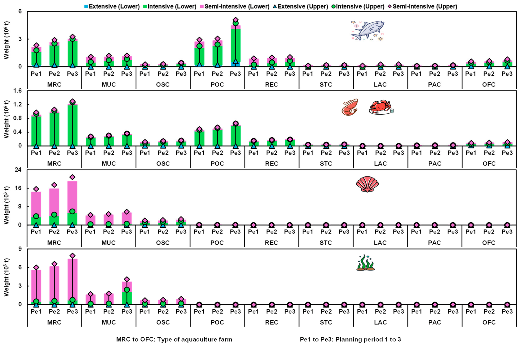
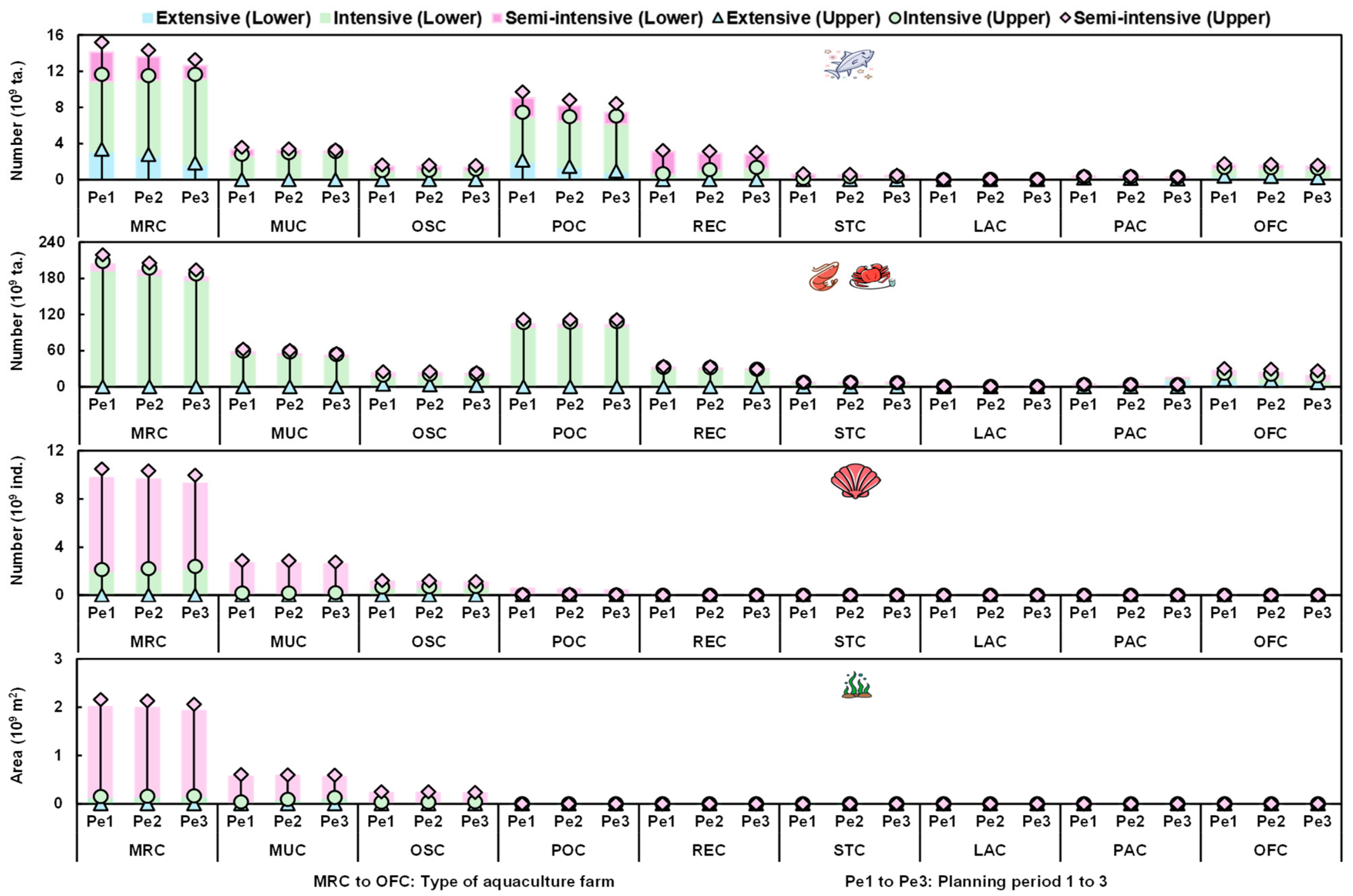
Figure 2 and Figure 3 present the optimal seed input and product output across the three planning periods (Pe1–Pe3), showing decreasing and increasing trends over time, respectively. The seed input achieves average total decrement rates of [2.86, 3.12]% (Pe1→Pe2) and [4.38, 4.87]% (Pe2→Pe3); and the product output achieves average total growth rates of [10.66, 11.78]% (Pe1→Pe2) and [24.36, 27.87]% (Pe2→Pe3). This reveals an obvious rise in the product output/seed input ratio (i.e., a slower increase in the seed input and a faster expansion of the product output), indicating that the province could further scale up aquaculture production. The changes depend on the live-weight of aquaculture species, which is associated with improved farming conditions such as abundant nutrients, excellent species, etc. Shellfish and algae would jointly contribute [75.02, 77.32]% to total product output in Pe1, [74.58, 75.70]% in Pe2, and [72.12, 73.45]% in Pe3. Despite a mild declining tendency, they would still play a significant role in the provincial aquaculture industry.
Given Fujian’s endowment of both freshwater and marine aquaculture resources, all farming types would be deployed to facilitate the development of the four cultured species. MRC, MUC, and POC would dominate fish and shrimp–crab cultivation, contributing [74.92, 78.63]% and [80.11, 83.27]% to their respective total product outputs throughout the planning horizon. MRC, MUC. and OSC serve as the primary cultivation aquafarms for shellfish and algae, occupying [98.43, 99.13]% and [99.31, 99.98]% of their corresponding product outputs. Such a distribution is mainly constrained by the minimum and maximum live-weight and seed-quantity, as well as the water availability and space allowance. The findings suggest policymakers should prioritize quality control in MRC and MUC cultivation, followed by the effective management of POC and OSC. It is also shown that fish and shrimp–crab would be mainly cultured under the intensive mode, with the farming ratios averaging 58.99% and 92.76% in Pe1, then rising to 79.49% and 96.53% in Pe3. Shellfish and algae would be mainly cultured by the semi-intensive mode, with the farming ratios averaging 75.36% and 90.27% in Pe1 and then declining to 72.43% and 74.38% in Pe3, as the intensive mode would gradually be adopted to sustain a stable ecological environment and ensure excellent product quality.

3.2. Expanding Capacity to Support Electricity Consumption

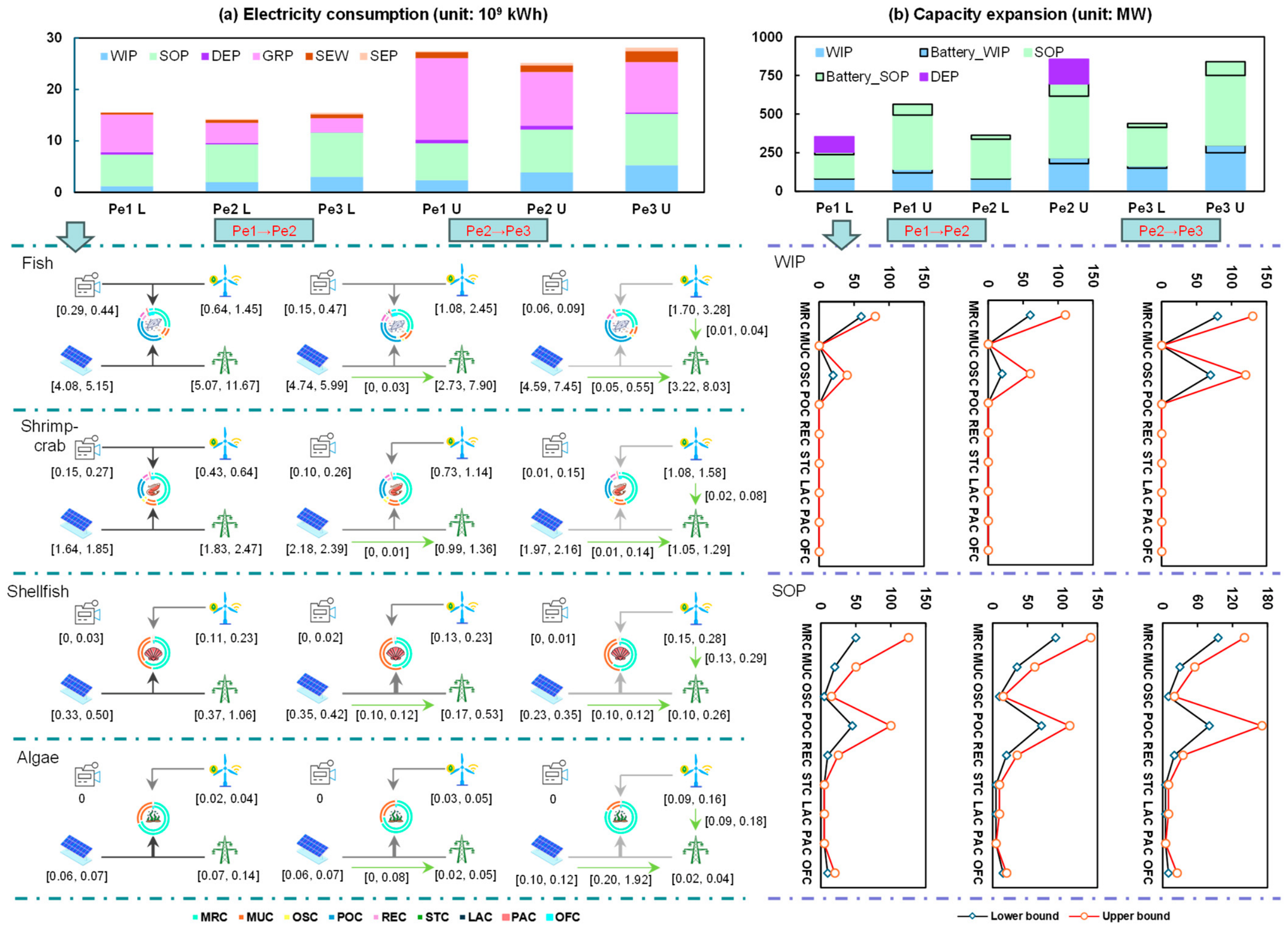
Figure 4 presents the electricity consumption and capacity expansion of renewable energy (i.e., wind power WIP and solar power SOP) from Pe1 to Pe3. The total electricity consumption would show an upward trend, driven by increasing aquaculture production scale. WIP and SOP would gradually replace the power grid (GRP) as the dominant electricity supply sources. In Pe1, they would account for [36.50, 48.50]% of the total electricity consumption, rising to [60.32, 81.05]% in Pe3, accompanied by substantial capacity expansion. By the end of the planning horizon, the installed capacities of WIP and SOP would reach [310, 550] MW (with [30, 110] MW battery) and [1000, 1550] MW (with [65, 240] MW battery), respectively. DEP (diesel power) would gradually be phased out.
Energy consumption patterns also differ notably across species: fish and shrimp–crab farms would occupy the largest share of total electricity consumption (about [93.72, 94.85]% over the three periods) due to the high electricity demand of the intensive mode (intensive feeding, water aeration, facility operation, etc.). MRC, MUC, and POC would drive a prominent increment of the WIP and SOP capacity, owing to the large production scale and superior construction conditions (e.g., topography, geology, water quality, wind and solar sources, etc.). In Pe3, their total WIP and SOP capacities would occupy approximately 100% and [77.65, 78.89]% of the overall installed capacity, respectively. These results reveal that the province should formulate policies and invest funds to shift the GRP-reliant energy structure towards a WIP–SOP-dominant energy structure, meeting the rising electricity demand and carbon emission mitigation requirement.

3.3. Regulating Flows to Support Water Consumption

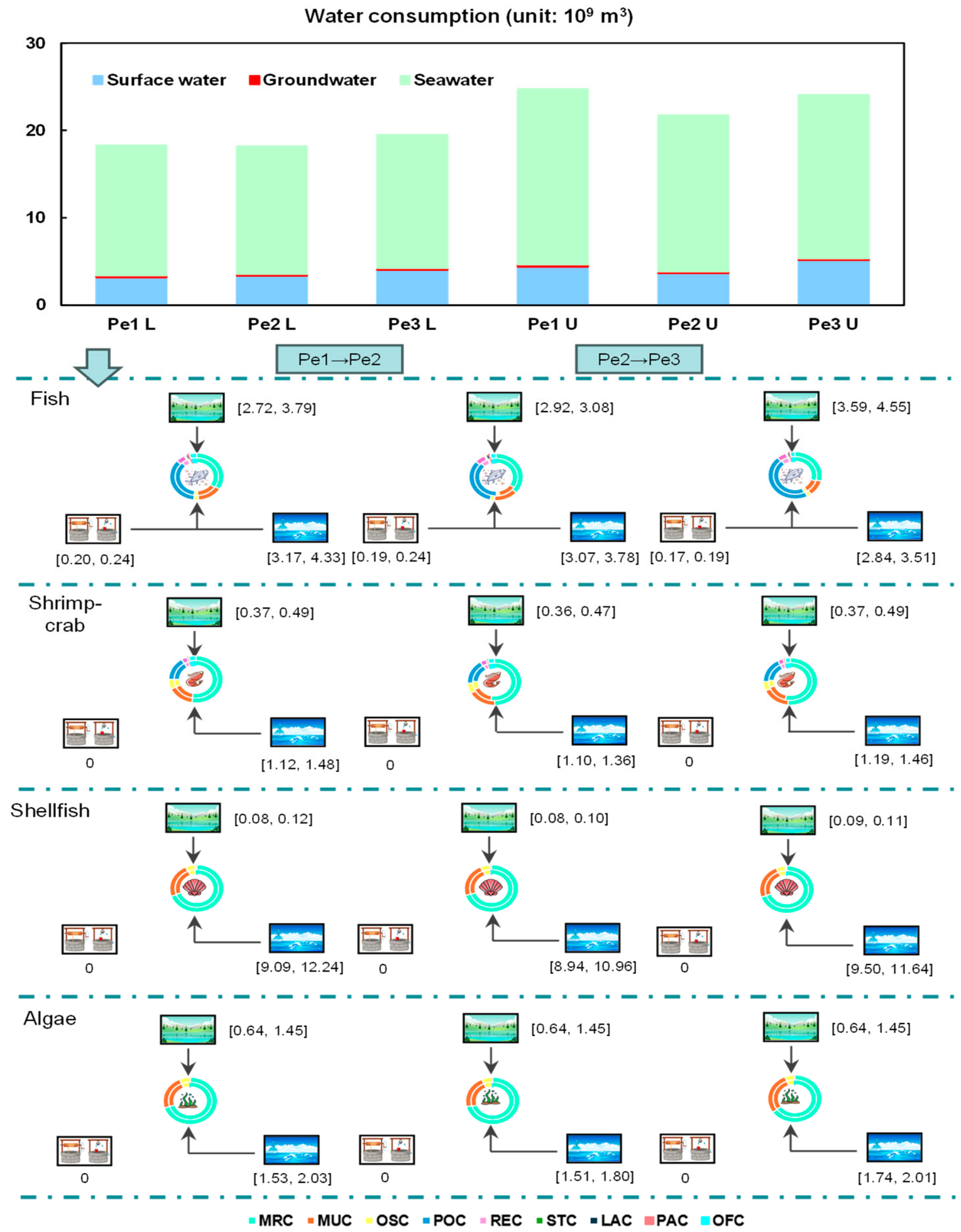
Figure 5 illustrates the water consumption from surface water, groundwater, and seawater across the three planning periods. It is important to interpret these quantities correctly. Surface water and groundwater represent consumptive freshwater withdrawal, i.e., water extracted and consumed during aquaculture operations.
The total water consumption for aquaculture would increase over time, driven by the expansion of aquaculture activities. Over the entire planning horizon, seawater would be the dominant source, occupying more than [80.14, 80.45]% of the total consumption; surface water consumption would remain relatively low and stable, representing about [18.65, 18.88]%; and groundwater consumption would be minimal and almost exclusively consumed by fish farms. The contribution of seawater to the total water consumption would increase from Pe1 to Pe3, highlighting the industry’s gradual shift toward marine-based aquaculture, which would help alleviate the pressure on freshwater resources. Seawater quantities represent exchange and circulation volumes rather than consumptive resource depletion. The large seawater exchange volumes reflect the scale of marine aquaculture production, particularly shellfish and algae farming. However, it should be emphasized that large seawater exchange volumes are not environmentally neutral. Their environmental acceptability depends on meeting water quality standards, particularly for TN, TP, SS, and COD concentrations in discharged tailwater. The model ensures that these discharge limits are satisfied (as discussed in Section 3.6), with exchange rates bounded by the nutrient-assimilative capacity of receiving water bodies.
Surface water and groundwater represent consumptive freshwater withdrawal, i.e., water that is extracted and consumed during aquaculture operations. The surface water allocation results indicate that the consumptive use of freshwater resources would increase over the planning horizon (reaching [4.05, 5.15] × 109 m3 in Pe3), driven primarily by pond culture (POC) expansion. Seawater quantities, by contrast, represent exchange or circulation volumes rather than consumptive use. The large seawater exchange volumes, over 80% of the total water use, reflect the scale of marine aquaculture production, particularly shellfish and algae farming, and should not be interpreted as resource depletion.
In terms of species-specific consumption, shellfish and algae farming would account for over [61.42, 61.47]% and [10.30, 10.63]% of the total seawater use, respectively, owing to their large-scale production and marine habitat adaptation. Fish farming would consume over [20.48, 20.81]% of the total seawater and [86.28, 87.09]% of the total surface water, corresponding to its production modes (e.g., INM) and farm types (e.g., MRC and POC). The distinction between consumptive freshwater use and seawater exchange is critical: while seawater exchange volumes are large in absolute terms, they impose minimal pressure on water resources compared to consumptive freshwater withdrawal. These results suggest that water allocation policies should prioritize shellfish and fish farms to meet their substantial demand, while maintaining attention to the water quality in aquaculture areas.

3.4. Aquafeed and Medicine Consumption

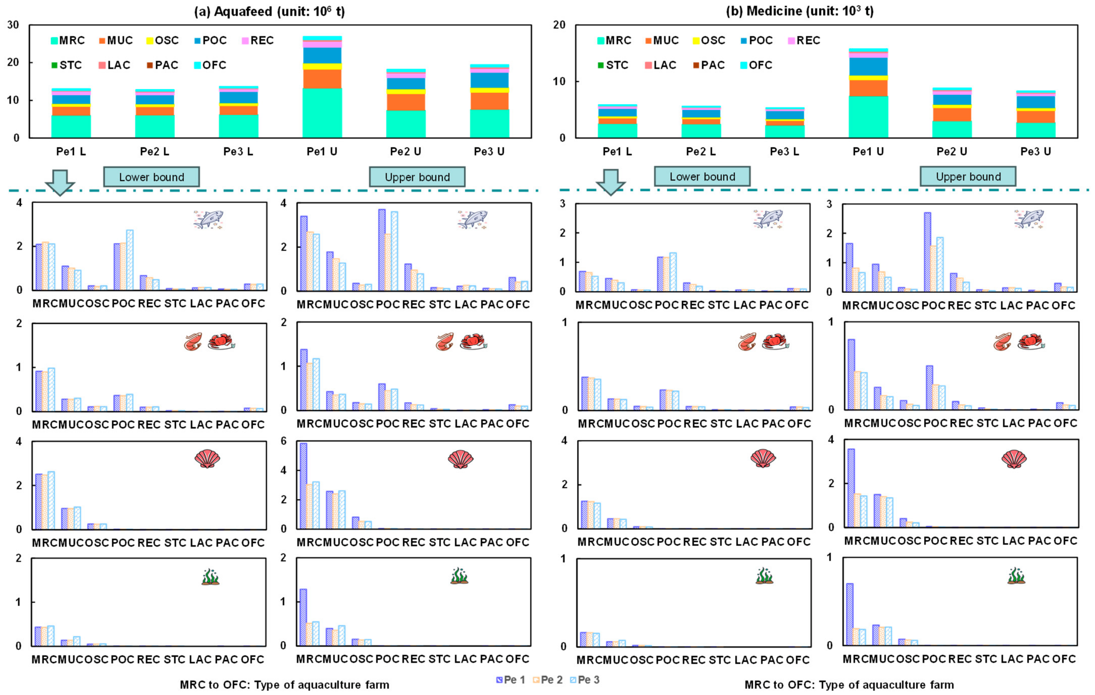
Figure 6 presents the consumption of aquafeed and medicine across different aquaculture farm types from Pe1 to Pe3. The total aquafeed consumption would show a slight upward trend at the lower bound (from approximately 12.34 × 10⁶ t to 14.28 × 10⁶ t) and a sharp decline at the upper bound (from 27.35 × 10⁶ t to 20.88 × 10⁶ t) over the same period. MRC and MUC would account for the largest shares (about [55.34, 60.03]% and [20.87, 24.38]%, respectively) attributable to their large cultivation scales. Fish and shellfish farming would be the dominant consumers of aquafeed, accounting for approximately [41.93, 48.35]% and [25.76, 34.45]%, respectively, owing to their high feeding requirements, high cultivation intensity, and/or large cultivation scales. In contrast, algae farming would rely on natural food sources, resulting in minimal or zero aquafeed consumption. The share of low-carbon aquafeed would increase from [16.43, 22.55]% in Pe1 to [45.35, 50.33]% in Pe3, contributing to carbon emission reduction.
Similarly, total medicine consumption would show a slight upward trend at the lower bound (around 5.65 × 10⁶ t) and a sharp decline at the upper bound (from 15.35 × 10⁶ t to 8.37 × 10⁶ t) from Pe1 to Pe3. All medicine quantities in this study are reported in 106 t (million tons). The highest consumption is concentrated in MRC, MUC, and POC, occupying more than 80.72% of the total consumption. Fish and shellfish farming would be the main consumers of aquaculture medicine, while shrimp–crab and algae farming show negligible medicine demand. These findings indicate that fish and shellfish farming in MRC, MUC, and POC should be monitored to prevent the overuse of medicine.
It is important to note that the medicine quantities represent the optimized allocation of veterinary products required to support the production targets under the model’s constraints. They are theoretical estimates rather than actual measurements of medicine residues in aquatic products. These results should not be interpreted as direct evidence of product safety, residue levels, or regulatory compliance. The primary purpose of including medicine in the model is to capture the material and cost implications of disease management in aquaculture.

3.5. Male and Female Structure

The inclusion of the female labor share in the model is justified as an exploratory proxy for social responsibility, specifically related to gender equality and inclusive employment. This aligns with the Guidelines for Sustainable Aquaculture [1] (FAO, 2025) and SDG 5 (Gender Equality). The data are derived from the Fujian Statistical Yearbook [34] and the China Fisheries Statistical Yearbook [33], which report the gender-disaggregated employment data for the aquaculture sector. However, it should be acknowledged that the female labor share indicator reflects the employment structure rather than a comprehensive measure of gender equality. It does not capture qualitative dimensions such as wage gaps, working conditions, career advancement, or decision-making power. Therefore, this indicator should be interpreted as a proxy for the employment structure, and future research should complement it with qualitative data on women’s empowerment in aquaculture.
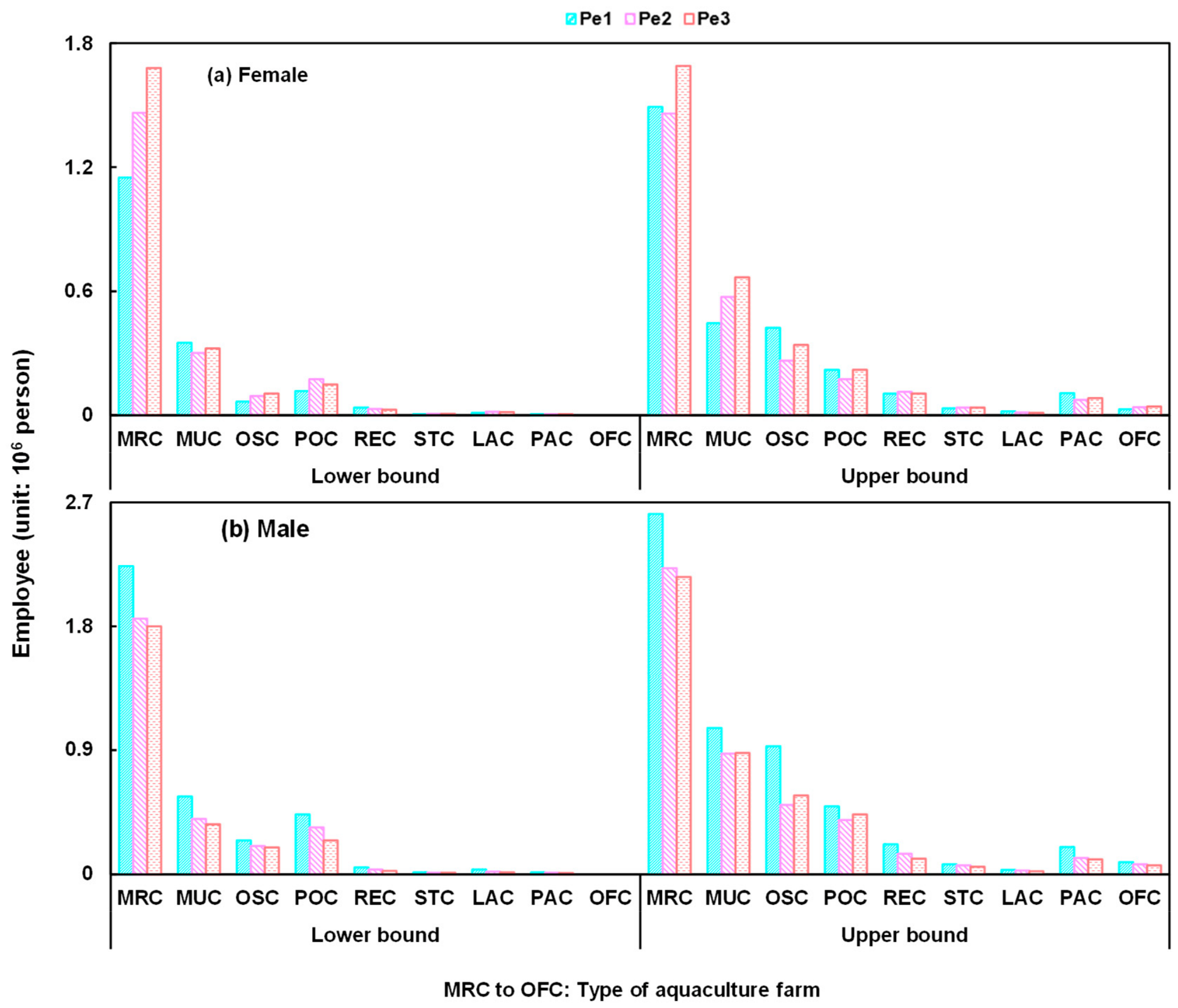
Figure 7 presents the optimized gender structure of employees across different aquaculture farm types from Pe1 to Pe3. MRC is the largest source of jobs for both genders, with female employment reaching approximately [1.22, 1.81] × 106 persons and male employment peaking at [2.12, 2.54] × 106 persons, far exceeding other farm types. Male employment is consistently higher than female employment across nearly all farm types, particularly in MRC and MUC. While male jobs in MRC show a slight downward trend from Pe1 to Pe3, they remain dominant. Female employment, also concentrated in MRC, shows a slight upward trend over the same period, with secondary contributions from MUC, POC, and OSC. This divergent trend, declining male employment alongside rising female employment, suggests the gradual progress toward a more balanced workforce participation. However, given the indicator’s limitations as a structural proxy, these results should be interpreted with caution; they indicate directional change rather than comprehensive gender equity. Future research should complement these findings with qualitative assessments of the working conditions, wage equity, and career advancement opportunities for women in aquaculture.

3.6. Pollutant and Carbon Emissions

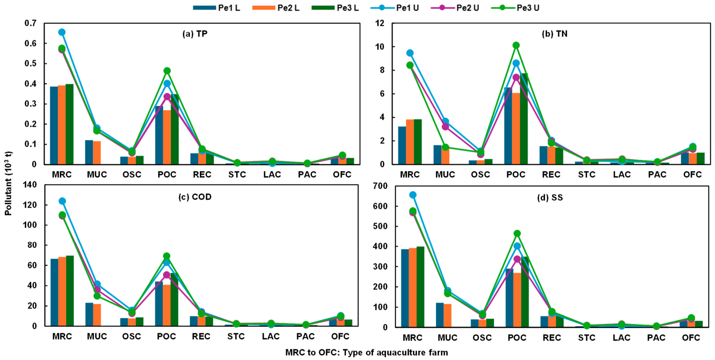
Figure 8 presents the optimized discharge levels of total nitrogen (TN), total phosphorus (TP), suspended solids (SS), and chemical oxygen demand (COD) from aquaculture tailwater from Pe1 to Pe3. Over the planning horizon, the lower bounds of pollutant discharges exhibit an increasing trend, while the upper bounds decline, leading to progressively narrower interval ranges. This convergence suggests a reduction in the parametric uncertainty, driven by improved feed practices, an enhanced treatment efficiency, and a more consistent system performance over time. On average, TN and TP show the most pronounced reductions, decreasing by approximately [22.5, 28.8]% and [18.3, 24.6]%, respectively, from Pe1 to Pe3. SS and COD also exhibit downward trends, with reductions of approximately [15.2, 20.7]% and [12.8, 18.5]%, respectively. This decline is primarily attributable to the increased adoption of low-carbon feed, improved feed conversion ratios, and the expansion of tailwater treatment facilities, particularly in MRC, MUC, and POC, which are the largest contributors to pollutant loads. All discharge levels remain within the regulatory limits set by the Fujian Aquaculture Sewage Water Discharge Standards. Indirect carbon emissions, which are mainly attributed to electricity generation, display a similar downward trajectory over the planning horizon (calculated based on the obtained results and emission coefficients; a dedicated figure for this aspect is not presented). In Pe1, emissions are dominated by diesel and grid power, accounting for approximately [7.41, 10.04]% of the total emissions from energy consumption. By Pe3, as the wind and solar power supply [60.32, 81.05]% of the total electricity, carbon emissions decline by approximately [28.23, 35.12]%. This reduction demonstrates that the renewable energy transition not only ensures electricity supply stability but also contributes substantially to climate change mitigation. Notably, algae and shellfish farming provide significant carbon sequestration benefits, offsetting approximately [10.0, 15.03]% of the emissions from energy consumption by Pe3. This finding aligns with previous studies highlighting the carbon sink capacity of shellfish–algal aquaculture systems.

3.7. Video and Image-Text

The inclusion of media episodes in the model is justified as an exploratory proxy for community acceptability and public awareness. This is supported by previous research indicating that public communication is critical for gaining and maintaining the “social license to operate” in aquaculture and natural resource management [31,48]. The media episode limits and communication index are derived from a historical trend analysis of the media coverage of aquaculture in Fujian Province (2020–2024), combined with API-based data extraction from major online news platforms and social media channels.
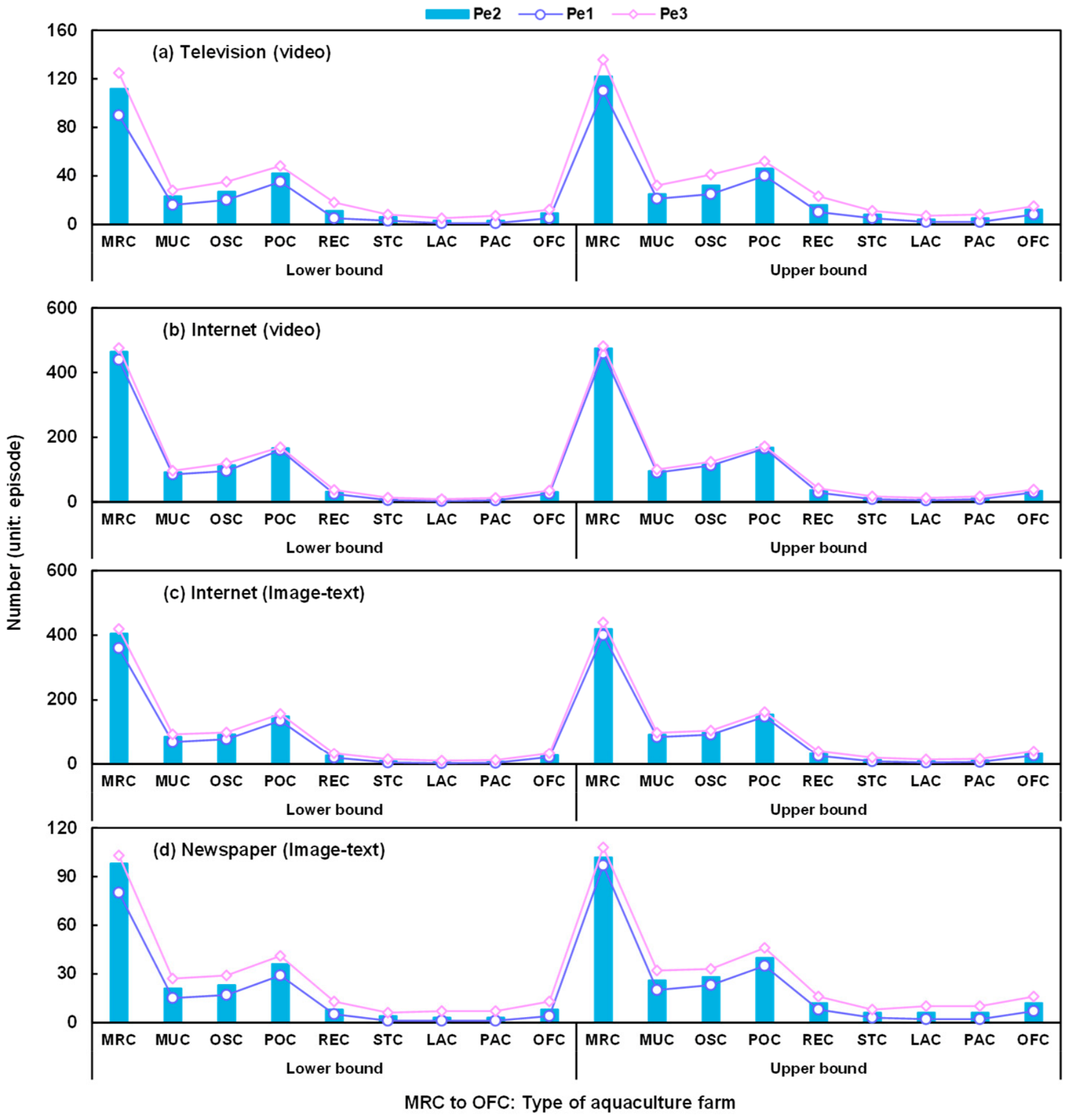
Figure 9 illustrates the number of media episodes (television video, Internet video, and Internet image-text) across different aquaculture farm types from Pe1 to Pe3. From Pe1 to Pe3, the total number of video and image-text episodes would rise considerably: the video episodes grow from [1016, 1100] to [1251, 1301], while image-text episodes would increase from [846, 991] to [1117, 1214]. This trend is primarily driven by two factors: the maximum allowable number of episodes and the communication index. The former is derived from the historical trend analysis of the media coverage of aquaculture in Fujian Province, while the latter reflects the system’s overall green and low-carbon development performance. A higher product output, lower pollutant and carbon emissions, lower resource consumption, and a more balanced gender structure contribute to a higher communication index.
The media allocation results indicate that MRC and POC are prioritized for promotion, occupying [48.61, 50.22]% and [17.58, 18.82]% of the total number of episodes, respectively. This concentration is attributable to the large production scale of MRC and the environmental sensitivity historically associated with POC, both of which justify greater public communication efforts. Internet-based platforms emerge as the preferred media channel due to their broad coverage, strong interactivity, low cost, and high dissemination efficiency. It is important to acknowledge that media episodes measure communication output, not communication effectiveness. The relationship between the media output and actual public perception is not linear and depends on the content quality, audience engagement, and socio-cultural context. The media allocation results should be interpreted as exploratory planning indicators rather than definitive measures of community acceptability.

3.8. Model Validation and Sensitive Analysis

To validate the IRAM and demonstrate the added value of the interval formulation, two complementary validation exercises were conducted. Historical baseline comparison: The model’s optimized output for the base year (2024) was compared with the observed aquaculture production in Fujian Province, which was reported as 9.25 × 10⁶ tons [32]. The IRAM-generated production estimate for 2024 is [9.55, 9.63] × 106 tons, yielding a deviation of approximately [3.24, 4.11]%. This minor deviation confirms the model’s capacity to replicate historical production levels, thereby enhancing confidence in its future projections. Deterministic counterpart comparison: To quantify the value of the interval programming approach, a deterministic version of the IRAM was constructed by fixing all interval parameters at their mid-point values. Under identical constraints, the deterministic model produced a single-point total system cost of 3.31 × 10¹² CNY, while the interval-based IRAM generated a range of optimal solutions ([2.81, 3.66] × 1012 CNY). More importantly, when subjected to uncertainty scenarios (e.g., ±15% variation in key parameters such as product demand and water availability), the deterministic model violated constraints in approximately 10% of the tested scenarios, whereas the IRAM maintained feasibility across all scenarios. This demonstrates that the interval formulation provides decision-makers with robust and flexible allocation plans that accommodate parameter variability, a critical advantage for long-term planning under uncertainty.
Given that the IRAM relies on a substantial number of interval parameters whose sources are described generically (e.g., estimated based on government reports, statistical yearbooks, etc.), a sensitivity analysis was conducted to test the robustness of the model’s conclusions to variations in interval width. The analysis followed a one-at-a-time approach, systematically varying the width of five key parameters, i.e., product demand, survival rates, aquaculture density, water availability, and unit costs, by ±5%, ±10%, and ±15% around their baseline interval bounds, while holding all other parameters constant. Combined scenarios were also tested, where all five parameters were simultaneously varied by ±10% and ±15%. The results indicate that the optimal system cost varies within a range of ±[2.21, 3.12]% under individual parameter variations of ±15%, and within ±[1.83, 3.22]% under combined ±15% variations, confirming that the model’s cost projections are stable and do not exhibit excessive sensitivity to reasonable changes in interval width. The resource allocation patterns across species and farm types remained qualitatively consistent across all scenarios. For instance, the dominance of MRC, MUC, and POC as the primary production areas persisted even under extreme parameter variations (±15%), indicating that the main policy recommendations are robust. Among the parameters tested, the product demand and survival rates were identified as the most sensitive, accounting for approximately 32.45% and 14.32% of the total variation in system cost, respectively. This suggests that future data collection and model refinement should prioritize these parameters to further enhance the model reliability. The sensitivity analysis also reveals that the interval formulation effectively accommodates parameter uncertainty: under combined ±15% variations, the IRAM maintained feasibility across all tested scenarios, highlighting its practical value for long-term planning under uncertain conditions.

3.9. Comparison with Previous Studies

The research findings illustrate that the IRAM provides a systematic framework for regional aquaculture resource allocation under uncertainty. The observed increase in the product output related to the seed input aligns with the productivity trends reported in recent aquaculture studies [11,15]. Nevertheless, this research extends the earlier models by integrating the energy, water, labor, feed, medicine, emissions, and communication constraints within a single regional optimization framework, a system boundary not previously handled at this scale. The renewable energy transition results are consistent with the water–energy–food nexus literature [21,22,24]; they further reveal that feasibility depends critically on regional characteristics such as resource availability, infrastructure, and sectoral competition.
The increasing share of female labor and the emphasis on media communication echo the growing recognition of social dimensions in sustainable aquaculture [4,5,31]. The IRAM demonstrates that these social factors can be operationalized as quantifiable optimization constraints, a methodological bridge between social science and operations research. The declining pollutant and carbon emission trajectories, driven by renewable energy penetration and improved feed practices, corroborate the carbon sequestration potential of shellfish and algae farming identified by Reference [44] and Reference [46], while also highlighting the need for an integrated tailwater treatment to meet the regulatory standards [43].
The IRAM not only confirms the trends observed in previous sectoral studies but also provides a holistic decision-support tool that enables policymakers to systematically evaluate trade-offs among competing sustainability objectives.

4. Conclusions and Policy Recommendations

This study proposes an inexact regional aquaculture system planning model (IRAM) to optimally allocate resources such as energy, water, labor, aquafeed, media, etc. for sustainable aquaculture activities (i.e., fish, shrimp–crab, shellfish, and algae culture). The objective of the IRAM is to minimize the system cost subject to multiple constraints, such as resource availability, demand–consumption balance, production–supply balance, pollutant and carbon emission mitigation, and the enhancement in the industry’s social recognition. The optimal solutions can be transformed into practical aquaculture resource allocation schemes to facilitate policy formulation for authorities. Specifically, the following conclusions represent model-based scenario insights derived under the specific assumptions and data conditions described in Section 2 and Section 3.
The application of the IRAM in Fujian Province (2026–2040, with each period covering 5 years) yields the following main findings:
(1)
The product output/seed input ratio of the four cultured species would obviously rise over periods, with an average growth rate of 3.76% (Pe1→Pe2) and 5.64% (Pe2→Pe3), revealing the reduced seed input and boosted harvest output. Such improvements stem from upgraded cultivation conditions such as the enriched nutrient aquafeed, enhanced rearing environment, expert-screened superior aquaculture varieties, etc.
(2)
MUC, MRC, and POC would still be the main farm types to culture the four species, accounting for over 72.36% to 91.23% of the total production of the four species. Such structures are attributed to the species’ rearing environment requirements, aquafarm expansion potential, aquafarm management convenience, etc.
(3)
Most fish and shrimp–crab would be cultured by the INM. The corresponding shares would, on average, rise from 58.99% in Pe1 to 79.49% in Pe3 for fish, and from 92.76% in Pe1 to 96.53% in Pe3 for shrimp–crab. Most shellfish and algae would be farmed by the SIM. The corresponding shares would decrease from 75.36% in Pe1 to 72.43% in Pe3 for shellfish, and from 90.27% in Pe1 to 74.38% in Pe3 for algae. These trends suggest a gradual transition toward more intensive practices for high-value species, driven by INM’s advantages in stable culture conditions, resource efficiency, and environmental control.
Based on the findings, some resource allocation policies are suggested as follows:
(1)
Energy: WIP and SOP would gradually replace GRP and DEP to become the dominant electricity supply sources, whose combined share would climb to [60.32, 81.05]% by Pe3. The corresponding installed capacity would rise to [310, 550] MW (mainly for MRC and OSC) and [1000, 1550] MW (mainly for MRC, MUC, and POC). This transition could contribute to reducing pollutant emissions and carbon emissions while supporting electricity supply stability, contingent on continued investment and favorable policy support.
(2)
Water: Water allocation would increase from [18.29, 24.72] × 109 m3 in Pe1 to [19.49, 24.05] × 109 m3 in Pe3, with surface water accounting for [17.57, 21.09]% and groundwater accounting for less than 1%. Surface water and groundwater represent consumptive freshwater withdrawal, whereas seawater represents the exchange/circulation volume rather than resource depletion. The increasing surface water allocation, reaching [4.05, 5.15] × 109 m3 in Pe3, is driven by pond culture expansion, indicating growing pressure on freshwater resources.
(3)
Aquafeed and medicine: The total aquafeed would be [13.01, 26.87] × 106 t in Pe1, [12.82, 18.17] × 106 t in Pe2, and [13.66, 19.42] × 106 t in Pe3, with the share of low-carbon aquafeed increasing to 52.25% in Pe3. The total medicine would be [5.85, 15.74] × 106 t in Pe1, [5.62, 8.83] × 106 t in Pe2, and [5.33, 8.31] × 106 t in Pe3. These quantities are theoretical estimates derived from the model’s constraints and should not be interpreted as direct evidence of product safety or residue control. Their primary purpose is to capture the material and cost implications of disease management.
(4)
Labor: Total labor would be [5.34, 8.58] × 106 person in Pe1, [4.97, 7.17] × 106 persons in Pe2, and [4.98, 7.61] × 106 person in Pe3, with the share of female labor increasing to about 44.48% in Pe3. This suggests potential improvements in the workforce gender balance, though the indicator reflects the employment structure rather than comprehensive gender equity.
(5)
Media: The video and image-text episodes would increase from [1016, 1100] and [846, 991] to [1251, 1301] and [1117, 1214], respectively, with MRC and POC receiving the highest allocation ([48.61, 50.22]% and [17.58, 18.82]%) via Internet-based platforms. The results suggest that media output may serve as a communication strategy to enhance community acceptability, subject to validation through field studies of public attitudes.
Despite the contributions of this study, several limitations still exist, which indicate promising directions for future research. The limitations are as follows:
(1)
The IRAM’s outputs depend on the accuracy and representativeness of the interval parameter estimates derived from statistical yearbooks, government reports, and literature sources;
(2)
Some exploratory indicators (e.g., media episodes and female labor share) have not been validated against empirical field data;
(3)
The interval programming approach captures parameter variability but does not address structural uncertainty or stochastic variability;
(4)
The planning horizon assumes stable economic, social, and environmental conditions, which may not hold under future climate or policy changes;
(5)
The findings are valid only under the scenario conditions specified in the model and may not be generalizable to other regions or time periods.
Despite these limitations, the IRAM provides a foundation for several promising research directions. The framework could be applied to other aquaculture-producing regions to test its generalizability. It could also be extended to include additional sustainability dimensions, such as biodiversity impacts, ecosystem service valuation, and climate change scenarios, and developed into a dynamic version incorporating real-time data for adaptive management. Furthermore, the media allocation results could be refined through a social media sentiment analysis to better capture the dynamics of the public discourse on aquaculture.

Supplementary Materials

The following supporting information can be downloaded at: https://www.mdpi.com/article/10.3390/su18178761/s1. Table S1: Features of aquaculture production modes; Content S2: Interval programming formulation and solution algorithm; Table S3. Additional data of main parameters.

Author Contributions

Conceptualization, software, and writing—original draft preparation, H.L.; investigation, data curation, and formal analysis, J.L. (Jiawei Li) and C.C.; visualization, supervision, and funding acquisition, X.L.; methodology, validation, and writing—review and editing, J.L. (Jing Liu) All authors have read and agreed to the published version of the manuscript.

Funding

This work was funded by the Xiamen Key Laboratory of Intelligent Fishery (No: XMKLIF-OP-202404), the Fujian Provincial Social Science Foundation Project (No: FJ2024B082), and Fujian Provincial Education Research Project for Young Teachers (No: JAT242024).

Institutional Review Board Statement

Not applicable.

Informed Consent Statement

No human subjects were involved in this study.

Data Availability Statement

The data presented in this study are derived from multiple sources. We are committed to making the complete dataset and model files available upon reasonable request to the corresponding author after internal review and authorization are completed. We anticipate that a publicly accessible repository will be established within 12 months following publication.

Acknowledgments

The authors are grateful to the editors and the anonymous reviewers for their insightful comments and suggestions.

Conflicts of Interest

The authors declare no conflicts of interest.

Appendix A. Parameter List

Subscripts:
aaquaculture species type, a = 1 for fish, a = 2 for shrimp–crab, a = 3 for shellfish, a = 4 for algae
kaquaculture area type, k = 1 for shallow-sea culture (MRC), k = 2 tidal-flat culture (MUC), k = 3 for offshore culture (OSC), k = 4 for pond culture (POC), k = 5 for reservoir culture (REC), k = 6 for stream culture (STC), k = 7 for lake culture (LAC), k = 8 for paddy culture (PAC), and k = 9 for other freshwater culture (OFC)
tplanning period, t = 1 for 2026–2030, t = 2 for 2031–2035, and t = 3 for 2036–2040; when t = 1, t − 1 = 0, which means, for the initial period, corresponding data is known
mcommunication type, m = 1 for video, m = 2 for image-text
Decision variables:
N F E a , k , t ± number of seed input of extensive mode (tail, tail, individual, and m2, abbreviated as ta., ta., ind., and m2)
N F S a , k , t ± number of seed input of semi-intensive mode (ta., ta., ind., and m2)
N F I a , k , t ± number of seed input of intensive mode (ta., ta., ind., and m2)
E W T a , k , t ± wind power electricity consumption, as WIP (kWh)
E P P a , k , t ± solar power electricity consumption, as SOP (kWh)
E D G a , k , t ± diesel power electricity consumption, as DEP (kWh)
E P G a , k , t ± grid power electricity consumption, as GRP (kWh)
S E W a , k , t ± wind power electricity selling to the grid, as SEW (kWh)
S E P a , k , t ± solar power electricity selling to grid, as SEP (kWh)
E B E a , k , t ± capacity of added diesel generators (kW)
N W E a , k , t ± number of newly-built wind turbines (unit)
E B P a , k , t ± capacity of added battery for storing wind power (kW)
P A E a , k , t ± area of newly-built photovoltaic panels (m2)
E S P a , k , t ± capacity of added battery for storing solar power (kW)
A S W a , k , t ± volume of surface water utilization (m3)
A G W a , k , t ± volume of groundwater utilization (m3)
A S E a , k , t ± volume of seawater utilization (m3)
T C F a , k , t ± mass of conventional bait feeding (kg)
T L F a , k , t ± mass of low-carbon bait feeding (kg)
T L M a , k , t ± mass of medicine feeding (kg)
L A F a , k , t ± number of female laborers (person)
L A M a , k , t ± number of male laborers (person)
N M E m , k , t ± number of promotional videos in social media (unit)
N E P m , k , t ± number of promotional news in newspaper (unit)
N T V m , k , t ± number of promotional videos on TV channels (unit)
Other parameters:
U C F a , k , t ± unit cost of purchasing seed (CNY/ta., ta., ind., and m2), CNY: Chinese Yuan
U C E a , k , t ± unit cost of excessive aquaculture facility expansion, without renewable energy cost (CNY/m2)
U C S a , k , t ± unit cost of semi-intensive aquaculture facility expansion, without renewable energy cost (CNY/m2)
U C I a , k , t ± unit cost of intensive aquaculture facility expansion, without renewable energy cost (CNY/m2)
W E S a , k , t ± unit cost of consuming wind power electricity (CNY/kWh)
B E S a , k , t ± unit cost of consuming solar power electricity (CNY/kWh)
D S E a , k , t ± unit cost of consuming diesel power electricity (CNY/kWh)
N P A a , k , t ± unit cost of purchasing grid power electricity (CNY/kWh)
B E E a , k , t ± unit income of selling wind power electricity (CNY/kWh)
B E P a , k , t ± unit income of selling solar power electricity (CNY/kWh)
I N B a , k , t ± unit cost of adding diesel generator (CNY/kW)
I N W a , k , t ± unit cost of building new wind turbine (CNY/unit)
I N P a , k , t ± unit cost of adding battery for storing wind power (CNY/kW)
I N E a , k , t ± unit cost of building new photovoltaic panel (CNY/m2)
I N S a , k , t ± unit cost of adding battery for storing solar power (CNY/kW)
C S W a , k , t ± unit cost of consuming surface water (CNY/m3)
C G W a , k , t ± unit cost of consuming groundwater (CNY/m3)
C S E a , k , t ± unit cost of consuming seawater (CNY/m3)
U O F a , k , t ± unit cost of purchasing conventional bait (CNY/kg)
U L F a , k , t ± unit cost of purchasing low-carbon bait (CNY/kg)
U L M a , k , t ± unit cost of purchasing medicine (CNY/kg)
U I C a , k , t ± unit income of each laborer (CNY/person)
U W T a , k , t ± unit cost of treating water (CNY/m3)
P C E t ± unit cost of mitigating carbon, e.g., carbon sink, carbon trading (CNY/kg C)
O C A a , k , t ± unit income of selling carbon sink quota (CNY/kg C)
U M E t ± unit cost of produce and upload videos (CNY/unit)
U E P t ± unit cost of published news article (CNY/unit)
U T V t ± unit cost of broadcasting videos on TV channels (CNY/unit)
I D E a , k , t ± aquaculture density of extensive mode (ta./m3, ta./m3, ind./m3, and kg/m3)
I D S a , k , t ± aquaculture density of semi-intensive mode (ta./m3, ta./m3, ind./m3, and kg/m3)
I D I a , k , t ± aquaculture density of intensive mode (ta./m3, ta./m3, ind./m3, and kg/m3)
H E I a , k , t ± water depth of aquaculture pond (m)
C D E t ± carbon emission coefficient of combusting diesel; “C” is carbon dioxide equivalent (kg C/kWh)
C O C a , k , t ± carbon sink ability of each aquaculture species (kg C/ta., kg C/ind., or kg C/m2)
N N S a , t ± minimum total number of aquaculture species (ta., ind., or kg)
A N S a , t ± maximum total number of aquaculture species (tail, ind., or kg)
W E L a , k , t ± average aquatic product weights with low weight-level (kg/ta., kg/ind., or kg/kg)
W E M a , k , t ± average aquatic product weights with medium weight-level (kg/ta., kg/ind., or kg/kg)
W E H a , k , t ± average aquatic product weights with high weight-level (kg/ta., kg/ind., or kg/kg)
I F D a , t ± minimum total live-weight (kg)
A F D a , t ± maximum total live-weight (kg)
U E E a , k , t ± unit amount of electricity consumption for culturing species (kWh/kg)
U E W a , k , t ± unit amount of electricity consumption for treating sewage (kWh/(m3·day))
U E L a , k , t ± amount of energy consumption per unit of labor (kWh/person)
A D E t ± amount of available diesel (kg)
E B a , k , t ± initial capacity of diesel generator (kW)
T I C a , k , t ± working time of diesel generator (hour)
F I L a , k , t ± employee ratio of extensive mode (person/kg)
F E L a , k , t ± employee ratio of semi-intensive mode (person/kg)
F S L a , k , t ± employee ratio of intensive mode (person/kg)
H Y F k , t ± mixed farming ratio of excessive mode (%)
H Y E k , t ± mixed farming ratio of semi-intensive mode (%)
H Y S k , t ± mixed farming ratio of intensive mode (%)
N W a , k ± number of wind turbines at the beginning of planning period
P W a , k , t ± rated power of wind turbine (kW)
W B a , k ± battery capacity of wind turbines at the beginning of planning period (kW)
W T a , k , t ± number of days without wind (day)
W D a , k , t ± working time of battery for wind power (hour/day)
T I W a , k , t ± working time of wind turbines (hour)
P A a , k ± area of photovoltaic panels at the beginning of planning period (m2)
G I a , k , t ± average daily global irradiance (kW/m2)
T I P a , k , t ± working time of photovoltaic panels (hour)
P B a , k ± battery capacity of photovoltaic panels at the beginning of planning period (kW)
Y T a , k , t ± number of days without sunshine (day)
W P a , k , t ± working time of battery for photovoltaic power (hour/day)
L M P k , t ± minimum capacity of wind power (kW)
L P P k , t ± minimum capacity of solar power (kW)
L E B k , t ± minimum capacity of diesel power (kW)
U W P k , t ± maximum capacity of wind power (kW)
U P P k , t ± maximum capacity of solar power (kW)
U E B k , t ± maximum capacity of diesel power (kW)
U W W k , t ± water requirement of generating wind electricity (m3/kWh)
U W S k , t ± water requirement of generating solar electricity (m3/kWh)
U W A a , k , t ± water requirement per unit labor (m3/person)
A R W t ± available agricultural water (m3)
M S E k , t ± available seawater (m3)
A R E k , t ± maximum available area (m2)
U A W k , t ± area requirement per wind turbine, considering the distance between wind turbines (m2/unit)
U A P k , t ± area requirement per unit of photovoltaic panel (m2/m2)
U L O k , t ± area requirement per person (m2/person)
U B L a , k , t ± bait requirement of low live-weight level aquaculture product (kg/kg)
U B M a , k , t ± bait requirement of medium live-weight level aquaculture product (kg/kg)
U B H a , k , t ± bait requirement of high live-weight level aquaculture product (kg/kg)
U M L a , k , t ± medicine requirement of low live-weight level aquaculture product (kg/kg)
U M M a , k , t ± medicine requirement of medium live-weight level aquaculture product (kg/kg)
U M H a , k , t ± medicine requirement of high live-weight level aquaculture product (kg/kg)
A L M t ± allowable medicine (kg)
M W I t ± minimum investment for paying wages (CNY)
M W A t ± maximum investment for paying wages (CNY)
T N D k , t ± mass of allowable TN discharge (kg)
T P D k , t ± mass of allowable TP discharge (kg)
T S D k , t ± mass of allowable SS discharge (kg)
T C D k , t ± mass of allowable OC discharge (kg)
N O t ± NOx emission coefficient of combusting diesel (kg/kWh)
S O t ± SO2 emission coefficient of combusting diesel (kg/kWh)
P M t ± PM emission coefficient of combusting diesel (kg/kWh)
T N O t ± mass of allowable NOx emission (kg)
T P M t ± mass of allowable PM emission (kg)
T S O t ± allowable SO2 emission (kg)
T C O t ± direct and indirect carbon emission control (kg C)
M N M k , t ± minimum the number of promotional videos in social media (unit)
M E P k , t ± minimum the number of promotional news in newspaper (unit)
M T V k , t ± minimum the number of promotional videos on TV channels (unit)
T M N k , t ± maximum total number of videos and news (unit)
M X C t ± maximum investment to popularize modern aquaculture (CNY)
S U F a , k , t ± survival rate of aquaculture species under extensive mode (%)
S U S a , k , t ± survival rate of aquaculture species under semi-intensive mode (%)
S U I a , k , t ± survival rate of aquaculture species under intensive mode (%)
T E Y a , k , t ± retired diesel electricity generator ratio (%)
T W Y a , k , t ± retired wind turbines ratio (%)
T W S a , k , t ± retired battery ratio for storing wind power (%)
T P Y a , k , t ± retired photovoltaic panels ratio (%)
T P S a , k , t ± retired battery ratio for storing photovoltaic power (%)
M S t ± ratio of available surface water to available agricultural water (%)
M G t ± ratio of available groundwater to available agricultural water (%)
P D E t ± cost of purchasing diesel (CNY/ton)
T D C t ± allowable direct carbon emission (kg C)
L G H k , t ± communication index
R I M k , t ± minimum number of videos and image-text spreading by social media
R I T k , t ± minimum number of videos spreading by TV
L t length of each period (day)
η t ± electricity generation efficiency for consuming diesel (kWh/kg)
d x t period coefficient, equal to 1 (day)
c b n t ± mass of total nitrogen (i.e., TN) discharge per unit mass of bait (kg N/kg bait)
c m n t ± mass of TN discharge per unit mass of medicine (kg N/kg medicine)
o n t ± mass of TN discharge per unit volume of sewage, derived from excreta, sediment, etc. (kg N/m3 sewage)
c b p t ± mass of TP discharge per unit mass of bait (kg P/kg bait)
c m p t ± mass of TP discharge per unit mass of medicine (kg P/kg medicine)
o p t ± mass of TP discharge per unit volume of sewage, derived from excreta, sediment, etc. (kg P/m3 sewage)
c b s t ± mass of suspended solids (i.e., SS) discharge per unit mass of bait (kg SS/kg bait)
c m s t ± mass of SS discharge per unit mass of medicine (kg SS/kg medicine)
o s t ± mass of SS discharge per unit volume of sewage, derived from excreta, sediment, etc. (kg SS/m3 sewage)
c b c t ± mass of organic carbon (i.e., OC) discharge per unit mass of bait (kg OC/kg bait)
c m c t ± mass of OC discharge per unit mass of medicine (kg OC/kg medicine)
o c t ± mass of OC discharge per unit volume of sewage, derived from excreta, sediment, etc. (kg OC/m3 sewage)
h e a , k , t ± water recycle rate of extensive mode (%/day)
x r a , k , t ± water recycle rate of extensive mode (%/day)
h s a , k , t ± water exchange rate of semi-excessive mode (%/day)
h i a , k , t ± water exchange rate of intensive mode (%/day)
α k , t ratio of actual aquaculture area to the theoretical aquaculture pond for excessive mode (%)
β k , t ratio of actual aquaculture area (including the area of aquaculture pond, staff office, seeding room, etc.) to the theoretical aquaculture pond for semi-intensive mode (%)
γ k , t ratio of actual aquaculture area (including the area of aquaculture pond, staff office, seeding room sewage treatment pond, etc.) to the theoretical aquaculture pond for intensive mode (%)
r l t ± water utilization ratio of laborers’ daily life (%)
λ k , t ± maximum proportion of species cultured by extensive mode (%)
λ k , t ± minimum proportion of species cultured by intensive mode (%)
w l a , k , t ± ratio of aquaculture species with low weight-level (%)
w m a , k , t ± ratio of aquaculture species with medium weight-level (%)
w h i , k , t ± ratio of aquaculture species with high weight-level (%)
μ a , k , t ± working efficiency of photovoltaic panel (%)
ς t ± minimal renewable energy ratio (%)
σ t ± maximal renewable energy ratio (%)
φ k , t min minimum energy storage ratio of wind power (%)
φ k , t max maximum energy storage ratio of wind power (%)
ξ k , t min minimum storage ratio of solar power (%)
ξ k , t max maximum energy storage ratio of solar power (%)
l e t ± proportion of resources zone area in total area (%)
l a t ± proportion of office zone area in total area (%)
l s t ± proportion of sewage zone area in total area (%)
ω t ± minimum low-carbon bait ratio (%)
ϑ t ± proportion of female laborers (%)
r n a , k , t ± TN removal rate (%)
r p a , k , t ± TP removal rate (%)
r s a , k , t ± SS removal rate (%)
r c a , k , t ± OC removal rate (%)
υ t ± carbon sink trading ratio (%)
w 1 , k , t ± weight of product output level (%)
w 2 , k , t ± weight of TN emission level (%)
w 3 , k , t ± weight of TP emission level (%)
w 4 , k , t ± weight of SS emission level (%)
w 5 , k , t ± weight of COD emission level (%)
w 5 , k , t ± weight of carbon emission level (%)

References

  1. Food and Agriculture Organization of the United Nations (FAO). The State of World Fisheries and Aquaculture 2024: Blue Transformation in Action; Food and Agriculture Organization of the United Nations (FAO): Rome, Italy, 2024. [Google Scholar]
  2. de Melo, A.M.; Kosten, S.; Duque, V.L.D.; Santos, A.A.O.; Amado, A.M.; Soranço, L.C.; Dreise, J.; Martins, A.C.; Nasário, J.; Barbosa, A.P.D.; et al. Low carbon footprint of Nile tilapia farming with recirculation aquaculture. Resour. Conserv. Recycl. 2025, 217, 108201. [Google Scholar] [CrossRef] [Scilit]
  3. Food and Agriculture Organization of the United Nations (FAO). Guidelines for Sustainable Aquaculture (GSA); Food and Agriculture Organization of the United Nations (FAO): Rome, Italy, 2025. [Google Scholar]
  4. Shepon, A.; Gephart, J.A.; Golden, C.D.; Henriksson, P.J.G.; Jones, R.C.; Koehn, J.Z.; Eshel, G. Exploring sustainable aquaculture development using a nutrition-sensitive approach. Glob. Environ. Change 2021, 69, 102285. [Google Scholar] [CrossRef] [Scilit]
  5. Boyd, C.E.; Mcnevin, A.A. Resource use and pollution potential in feed-based aquaculture. Rev. Fish. Sci. Aquac. 2024, 32, 306–333. [Google Scholar] [CrossRef] [Scilit]
  6. Yang, J.; Wang, J.; Ma, K.; Zhang, Q.; Ji, W.; Guo, S. A bi-level optimization model of integrated energy system considering waste treatment under uncertainty. Energy 2025, 332, 136810. [Google Scholar] [CrossRef] [Scilit]
  7. Granada, L.; Lopes, S.; Novais, S.C.; Lemos, M.F.L. Modelling integrated multi-trophic aquaculture: Optimizing a three trophic level system. Aquaculture 2018, 495, 90–97. [Google Scholar] [CrossRef] [Scilit]
  8. Saadaoui, H.; Espejo-Carpio, F.J.; Guadix, E.M.; Ben Amar, R.; Pérez-Gálvez, R. Bi-objective optimization of tuna protein hydrolysis to produce aquaculture feed ingredients. Food Bioprod. Process. 2019, 115, 26–35. [Google Scholar] [CrossRef] [Scilit]
  9. Grasberger, J.; Forbush, D. Investigating a renewable-resource-targeting mobile aquaculture system using route optimization based on optimal foraging theory. J. Mar. Sci. Eng. 2023, 11, 2123. [Google Scholar] [CrossRef] [Scilit]
  10. Domínguez-May, R.; Hernández, J.M.; Velázquez-Abunader, I. A review of dynamic optimization in aquaculture production economics. Rev. Aquac. 2024, 16, 1696–1717. [Google Scholar] [CrossRef] [Scilit]
  11. Luna, M.; Llorente, I.; Cobo, A. Aquaculture production optimisation in multi-cage farms subject to commercial and operational constraints. Biosyst. Eng. 2020, 196, 29–45. [Google Scholar] [CrossRef] [Scilit]
  12. Nguyen, N.T.; Matsuhashi, R.; Vo, T.T.B.C. A design on sustainable hybrid energy systems by multi-objective optimization for aquaculture industry. Renew. Energy 2021, 163, 1878–1894. [Google Scholar] [CrossRef] [Scilit]
  13. Li, H.; Chatzifotis, S.; Lian, G.P.; Duan, Y.Q.; Li, D.L.; Chen, T. Mechanistic model based optimization of feeding practices in aquaculture. Aquac. Eng. 2022, 97, 102245. [Google Scholar] [CrossRef] [Scilit]
  14. Liu, Y.; Xu, X.; Xu, L.X.; Liu, Y.B.; Yang, N.; Jawad, S.; Luo, Y.C.; Liu, J.Y.; Hu, W.H. Collaborative water-electricity operation optimization of a photovoltaic/pumped storage-based aquaculture energy system considering water evaporation effects. Renew. Energy 2024, 237, 121886. [Google Scholar] [CrossRef] [Scilit]
  15. Zhang, R.S.; Chen, T.; Wang, Y.; Short, M. An optimisation approach for the design and operation of recirculating aquaculture systems integrated with sustainable hybrid energy systems. J. Clean. Prod. 2024, 477, 143860. [Google Scholar] [CrossRef] [Scilit]
  16. Dolatabadi, S.; Ricardez-Sandoval, L. Integration of process design and control of a pilot-scale recirculating aquaculture system. Aquac. Eng. 2025, 111, 102580. [Google Scholar] [CrossRef] [Scilit]
  17. Li, M.; Zhao, L.; Zhang, C.; Liu, Y.; Fu, Q. Optimization of agricultural resources in water-energy-food nexus in complex environment: A perspective on multienergy coordination. Energy Convers. Manag. 2022, 258, 115537. [Google Scholar] [CrossRef] [Scilit]
  18. Yu, B.; Bi, X.; Liu, X.; Sun, H.; Buysse, J. Exploring the application and decision optimization of climate-smart agriculture within land-energy-food-waste nexus. Sustain. Prod. Consum. 2024, 50, 536–555. [Google Scholar] [CrossRef] [Scilit]
  19. Zhu, X.; Su, X.; Chu, J.; Singh, V.P.; Wu, H.; Niu, J.; Wu, L. Improving synergy of the water-agriculture-ecology system in arid areas using a novel co-optimization model. Agric. Water Manag. 2025, 312, 109408. [Google Scholar] [CrossRef] [Scilit]
  20. Li, M.; Sun, H.; Liu, D.; Singh, V.P.; Fu, Q. Multi-scale modeling for irrigation water and cropland resources allocation considering uncertainties in water supply and demand. Agric. Water Manag. 2021, 246, 106687. [Google Scholar] [CrossRef] [Scilit]
  21. Ren, H.; Liu, B.; Zhang, Z.; Li, F.; Pan, K.; Zhou, Z.; Xu, X. A water-energy-food-carbon nexus optimization model for sustainable agricultural development in the Yellow River Basin under uncertainty. Appl. Energy 2022, 326, 120008. [Google Scholar] [CrossRef] [Scilit]
  22. Yuan, M.; Zheng, N.; Yang, Y.; Liu, C. Robust optimization for sustainable agricultural management of the water-land-food nexus under uncertainty. J. Clean. Prod. 2023, 403, 136846. [Google Scholar] [CrossRef] [Scilit]
  23. Li, D.; Zuo, Q.; Jiang, E.; Zhang, Z.; Wu, Q.; Wang, Y. An integrated water resources management model considering carbon source and sink under uncertainty: A case study of agricultural water-dominated basin. J. Clean. Prod. 2024, 436, 140667. [Google Scholar] [CrossRef] [Scilit]
  24. Feng, T.; Zhou, Z.; Liu, B.; Ren, H.; Zhu, Y.; Zhang, Y. A resource bi-level optimization model of water-energy-food-carbon nexus in a regional agricultural system under multi-stakeholder conditions. Renew. Energy 2025, 241, 122321. [Google Scholar] [CrossRef] [Scilit]
  25. Pokharna, N.; Tripathi, I.P. A generalized division approach for interval fractional programming problems. Appl. Math. Model. 2025, 144, 116048. [Google Scholar] [CrossRef] [Scilit]
  26. Pour, S.H.; Fard, O.S.; Zeng, B. A grey prediction model based on Von Bertalanffy equation and its application in energy prediction. Eng. Appl. Artif. Intell. 2025, 143, 110012. [Google Scholar] [CrossRef] [Scilit]
  27. Wang, S.Y.; Huang, G.H.; Zhou, X.; Tian, C.Y. A dual-interval fractional energy systems optimization for Nova Scotia, Canada. Renew. Sustain. Energy Rev. 2025, 212, 115455. [Google Scholar] [CrossRef] [Scilit]
  28. Song, X.L.; Wu, H.; Zhang, J.L.; Zhao, C.D.; Peña-Mora, F. Optimal operation of shared energy storage-assisted wind-solar-thermal power generation systems under the electricity-carbon markets. Energy 2025, 330, 136614. [Google Scholar] [CrossRef] [Scilit]
  29. Sun, L.; Dai, S.Y.; Tian, L.Y.; Ni, Z.C.; Lu, S.Y.; Yao, Y.R. Optimal water allocation considering water diversion projects in an agricultural irrigation district. Agriculture 2025, 15, 949. [Google Scholar] [CrossRef] [Scilit]
  30. Vasquez-Mejia, C.M.; Shrivastava, S.; Gudjónsdóttir, M.; Manzardo, A.; Ögmundarson, O. Current status and future research needs on the quantitative water use of finfish aquaculture using Life Cycle Assessment: A systematic literature review. J. Clean. Prod. 2023, 425, 139009. [Google Scholar] [CrossRef] [Scilit]
  31. Fudge, M.; Higgins, V.; Vince, J.; Rajaguru, R. Social acceptability and the development of commercial RAS aquaculture. Aquaculture 2023, 568, 739295. [Google Scholar] [CrossRef] [Scilit]
  32. Fujian Provincial Department of Ocean and Fisheries (FPOF). Aquaculture Product Bulletins; Fujian Provincial Department of Ocean and Fisheries (FPOF): Fuzhou, China, 2024. [Google Scholar]
  33. Ministry of Agriculture and Rural Affairs of the People’s Republic of China (MARC). China Fisheries Statistical Yearbook; China Agriculture Press: Beijing, China, 2024. [Google Scholar]
  34. Fujian Provincial Bureau of Statistics (FPBS). Fujian Statistical Yearbook; China Statistics Press: Beijing, China, 2024. [Google Scholar]
  35. Fujian Provincial People’s Government (FPPG). Fujian Provincial 14th Five-Year Special Energy Development Plan; Fujian Provincial People’s Government (FPPG): Fuzhou, China, 2022. [Google Scholar]
  36. Cheng, Y.; Jin, L.; Yan, Y.; Bai, R.; Wei, Y.; Huang, G. An improved fuzzy sorting algorithm coupling bi-level programming for synergetic optimization of agricultural water resources: A case study of Fujian Province, China. J. Environ. Manag. 2022, 312, 114946. [Google Scholar] [CrossRef] [Scilit] [PubMed]
  37. Fujian Provincial Department of Water Resources (FWDR). Fujian Province Water Resources Bulletin; Fujian Provincial Department of Water Resources (FWDR): Fuzhou, China, 2024. [Google Scholar]
  38. Xu, Y.; Huang, G.; Liu, Y.; Chen, L. Exploring the role of negative emission technologies in regional power system planning toward carbon net zero-A case study for the province of Saskatchewan, Canada. Energy 2025, 326, 136351. [Google Scholar] [CrossRef] [Scilit]
  39. Ma, Y.; Liu, Y.; Zhang, Q.; Li, Y.; Huang, G. Full-chain optimization of China’s net-zero emissions energy system toward 2060. Resour. Conserv. Recycl. 2025, 222, 108485. [Google Scholar] [CrossRef] [Scilit]
  40. Zoli, M.; Bacenetti, J. Energy analysis in fish aquaculture: Cumulative energy demand of different farming systems. Aquac. Eng. 2025, 110, 102525. [Google Scholar] [CrossRef] [Scilit]
  41. Rong, F.; Liu, H.; Zhu, J.; Qin, Q. Carbon footprint of shrimp (Litopenaeus vannamei) cultured in recirculating aquaculture systems (RAS) in China. J. Clean. Prod. 2024, 510, 145606. [Google Scholar] [CrossRef] [Scilit]
  42. Chairat, S.; Regmi, S.; Cheng, H.; Vongmahadlek, P.; Gheewala, S.H. Life cycle assessment of Tilapia production via conventional aquaculture and aquaponic systems. Aquaculture 2025, 208, 746760. [Google Scholar] [CrossRef] [Scilit]
  43. Fujian Provincial Department of Ecology and Environment (FDEE). Aquaculture Sewage Water Discharge Standards (DB35/2160-2023); Fujian Provincial Department of Ecology and Environment (FDEE): Fuzhou, China, 2023. [Google Scholar]
  44. Jia, R.L.; Li, P.; Chen, C.Z.; Liu, L.; Li, Z.H. Shellfish-algal systems as important components of fisheries carbon sinks: Their contribution and response to climate change. Environ. Res. 2023, 224, 115511. [Google Scholar] [CrossRef] [Scilit] [PubMed]
  45. Drizo, A.; Shaikh, M.O. An assessment of approaches and techniques for estimating water pollution releases from aquaculture production facilities. Mar. Pollut. Bull. 2023, 196, 115661. [Google Scholar] [CrossRef] [Scilit] [PubMed]
  46. Le, C.Y.; Feng, J.C.; Sun, L.W.; Yuan, W.Y.; Wu, G.Z.; Zhang, S.; Yang, Z.F. Co-benefits of carbon sink and low carbon food supply via shellfish and algae farming in China from 2003 to 2020. J. Clean. Prod. 2023, 414, 137436. [Google Scholar] [CrossRef] [Scilit]
  47. Li, K.; Jiang, R.T.; Qiu, J.Q.; Liu, J.L.; Shao, L.; Zhang, J.H.; Liu, Q.G.; Jiang, Z.J.; Wang, H.; He, W.H.; et al. How to control pollution from tailwater in large scale aquaculture in China: A review. Aquaculture 2024, 590, 741085. [Google Scholar] [CrossRef] [Scilit]
  48. Hervé-Bazin, C. (Ed.) Water Communication: Analysis of Strategies and Campaigns from the Water Sector; IWA Publishing: London, UK, 2014. [Google Scholar]
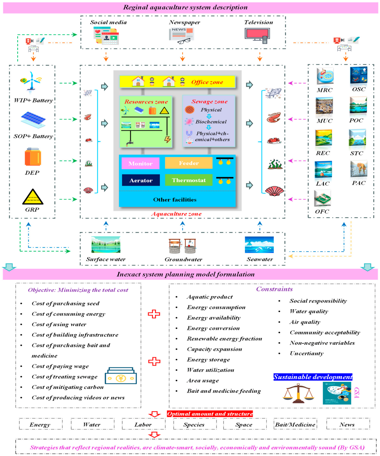
Figure 1. Framework of the IRAM.
Sustainability 18 08761 g001
Figure 2. Number (or area) of seed input.
Sustainability 18 08761 g002
Figure 3. Weight of product output.
Sustainability 18 08761 g003
Figure 4. Electricity consumption and capacity expansion.
Sustainability 18 08761 g004
Figure 5. Water consumption.
Sustainability 18 08761 g005
Figure 6. Amount of aquafeed and medicine.
Sustainability 18 08761 g006
Figure 7. Number of employees.
Sustainability 18 08761 g007
Figure 8. Pollutant emissions.
Sustainability 18 08761 g008
Figure 9. Number of video and image-text.
Sustainability 18 08761 g009
Table 1. Some economic, social, environmental parameters.
ParameterProduct or Aquafarm TypePlanning Period
t = 1 (Pe1)t = 2 (Pe2)t = 3 (Pe3)
Minimum product output
(109 kg)
Fish[7.53, 8.22][8.33, 9.25][10.55, 12.05]
Shrimp–crab[1.85, 2.06][2.08, 2.28][2.53, 2.67]
Shellfish[20.03, 21.15][21.85, 23.79][26.37, 28.96]
Algae[7.56, 8.12][8.34, 8.89][11.25, 12.06]
Unit cost of purchasing seeds
(CNY/ta., ta., ind., or m2)
Fish[0.45, 0.50][0.48, 0.53][0.51, 0.56]
Shrimp–crab[0.18, 0.26][0.21, 0.28][0.23, 0.30]
Shellfish[0.065, 0.072][0.068, 0.075][0.071, 0.078]
Algae[0.39, 0.65][0.43, 0.68][0.45, 0.70]
Maximum total number of videos and images
(Episode)
Shallow-sea culture[450, 500][505, 525][530, 550]
Tidal-flat culture[90, 110][115, 120][120, 130]
Offshore culture[100, 120][125, 130][131, 140]
Pond culture[170, 190][195, 205][205, 215],
Reservoir culture[30, 40][42, 45][46, 60]
Stream culture[8, 12][15, 20][24, 30]
Lake culture[5, 8][10, 15][18, 28]
Paddy culture[5, 10][12, 20][22, 30]
Other freshwater culture[28, 35][38, 45][50, 60]
Mass of allowable TN discharge
(106 kg)
Shallow-sea culture[3.87, 9.46][3.85, 9.12][3.84, 8.42]
Tidal-flat culture[1.65, 3.66][1.57, 3.20][0.55, 2.47]
Offshore culture[0.55, 1.13][0.51, 1.06][0.47, 1.02]
Pond culture[8.02, 10.63][7.88, 10.32][7.74, 10.11]
Reservoir culture[1.55, 2.04][1.52, 1.94][1.44, 1.82]
Stream culture[0.28, 0.42][0.26, 0.38][0.25, 0.35]
Lake culture[0.38, 0.50][0.32, 0.46][0.24, 0.41]
Paddy culture[0.21, 0.29][0.18, 0.27][0.16, 0.24]
Other freshwater culture[1.09, 1.53][1.05, 1.48][1.00, 1.45]
Minimum capacity of solar power (kW)Shallow-sea culture[40, 110][80, 120][90, 130]
Tidal-flat culture[10, 15][20, 40][30, 50]
Offshore culture[5, 10][10, 15][10, 20]
Pond culture[40, 90][60, 110][80, 140]
Reservoir culture[10, 20][20, 35][20, 35]
Stream culture[5, 10][5, 10][5, 10]
Lake culture[5, 10][5, 10][5, 10]
Paddy culture[5, 10][5, 10][5, 10]
Other freshwater culture[10, 20][15, 20][10, 25]
Disclaimer/Publisher’s Note: The statements, opinions and data contained in all publications are solely those of the individual author(s) and contributor(s) and not of MDPI and/or the editor(s). MDPI and/or the editor(s) disclaim responsibility for any injury to people or property resulting from any ideas, methods, instructions or products referred to in the content.