A Sequentially Coupled Econometric-Hydrological-Reduced-Form Economic Framework for Quantifying Global Water Demand and Economic Risks Through 2050

Abstract

Water scarcity threatens global stability, with demand set to surge 20–30% by 2050, pushing withdrawals from 4600 km³ yr⁻¹ today to 5500–6000 km³ yr⁻¹ under rising demographic and climatic pressures. This study presents a sequentially coupled econometric–hydrological–reduced-form economic framework that couples water supply dynamics with demand forecasting and macroeconomic impact assessment. Agriculture dominates current withdrawals at 70% (FAO AQUASTAT), followed by industry (20%) and domestic use (10%). Monte Carlo simulations (n = 1000) identify critical regional hotspots: Asia (stress ratio = 1.06), the Middle East (1.18), and Africa (0.99). The reduced-form economic module uses a target-calibrated scarcity elasticity (ε = 0.1865) applied against a fixed economic reference threshold (4600 km³ yr⁻¹). This internally calibrated parameter yields a first-order GDP loss estimate of approximately $16.0 trillion under the high-demand (+30%) 2050 scenario (6000 km³ yr⁻¹ demand), equivalent to 5.5% of projected 2050 global GDP ($290 trillion, PwC 2017 baseline). The resulting magnitude is broadly consistent with the order of GDP impacts discussed by OECD (2012) and GCEW (2024), although neither publication reports this specific elasticity value. This is not an independently predicted outcome; it is a calibrated scenario estimate produced by a reduced-form damage function designed to reproduce first-order magnitudes consistent with published structural model results. Mitigation strategies including efficiency improvements, pricing reforms, and AI-driven allocation can reduce demand by up to 40%, which within the model’s mathematical structure reduces the calibrated economic loss to zero. Sectoral water distribution is addressed through continuous linear programming with proportional rationing. This framework advances transparent, reproducible scenario-based understanding and informs policy decisions aimed at mitigating future water scarcity challenges globally, while explicitly acknowledging limitations relative to full structural CGE models and empirically estimated panel econometric models.

1. Introduction

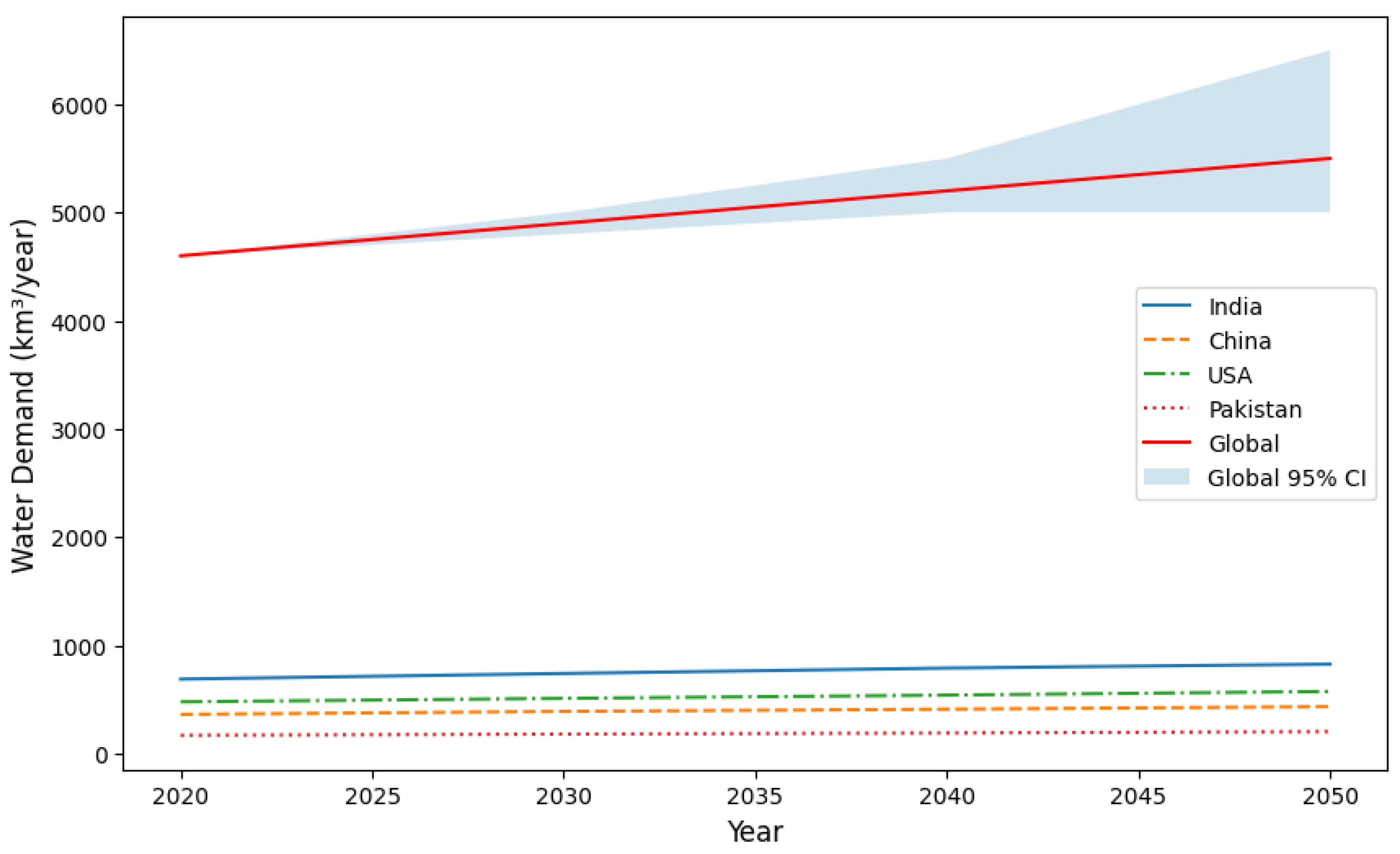
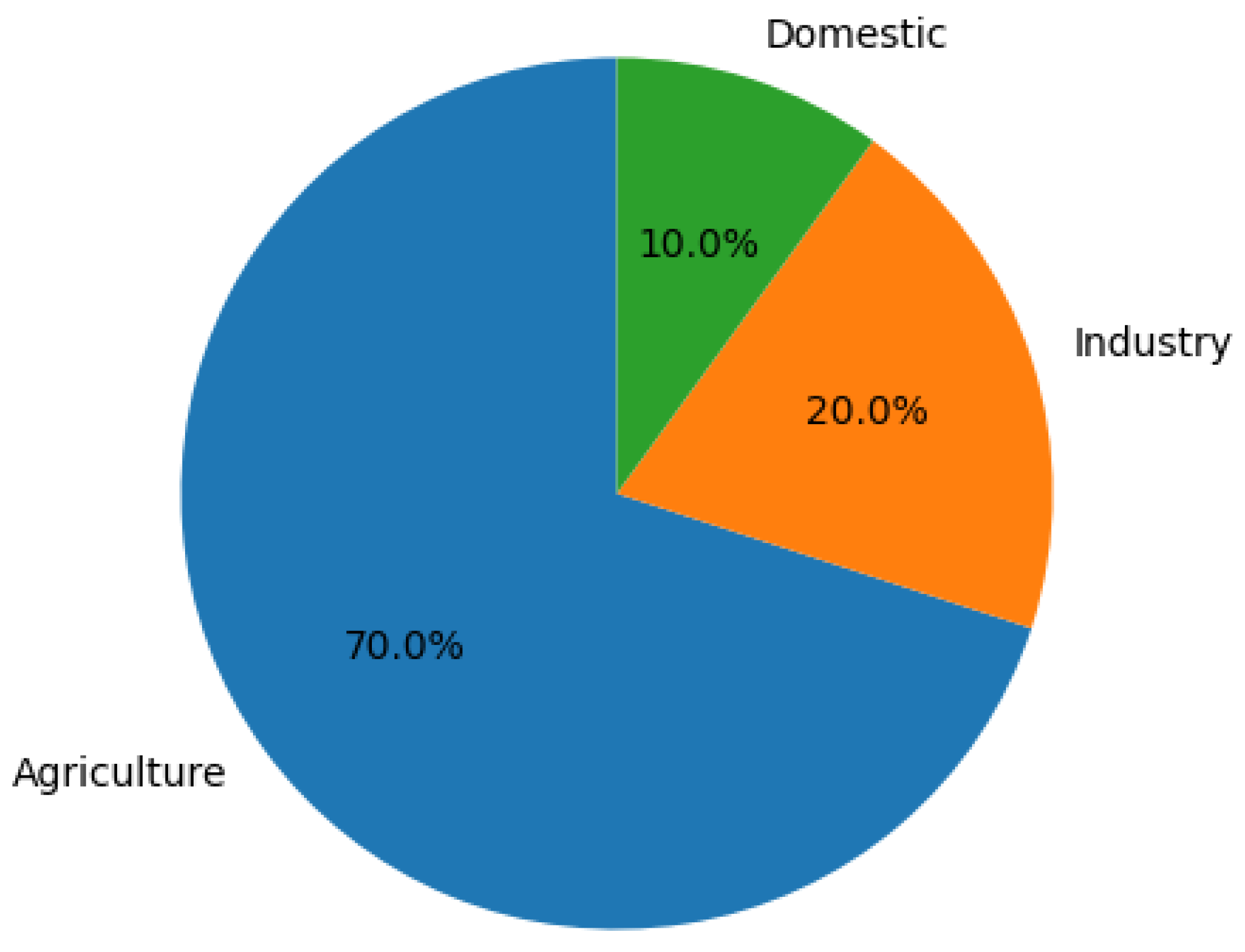
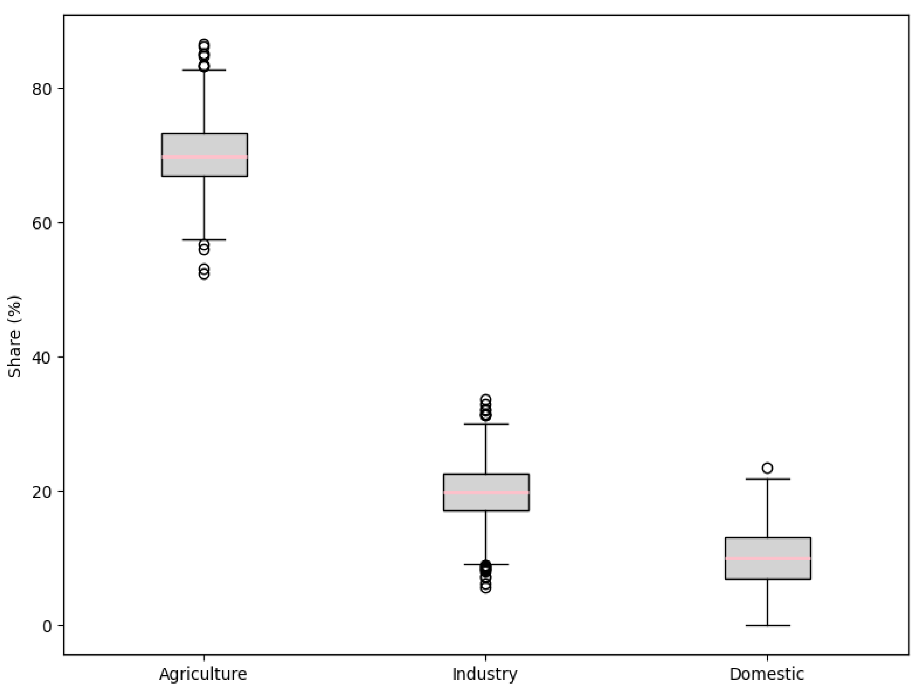
Global water demand has increased by approximately 600% over the past 100 years, reaching approximately 4600 km³ yr⁻¹ [1,2,3]. This escalation is primarily attributed to rapid population expansion, economic development, urbanization, and agricultural intensification, with agriculture accounting for about 70% of global withdrawals mainly for irrigation while industry and domestic uses contribute roughly 20% and 10%, respectively [2,3,4,5]. 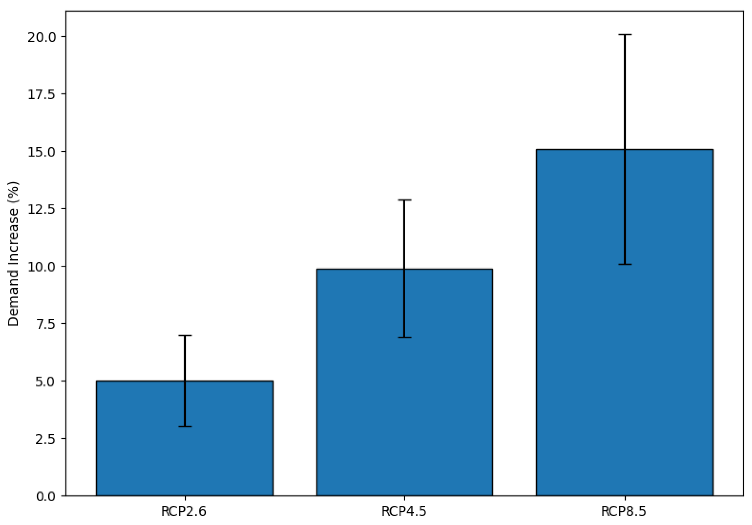In emerging economies, industrial and domestic demand is growing faster than agricultural demand, exacerbating regional disparities [4,5]. Projections suggest a 20–30% rise in overall demand by 2050, potentially reaching 5500–6000 km³ yr⁻¹, driven by a global population increase to between 9.4 and 10.2 billion people—a 22–32% rise with the majority of growth occurring in developing regions such as Sub-Saharan Africa (+108%) and Asia (+18%) [6]. The UN World Water Development Report (WWDR) [5] underscores that climate variability, including altered precipitation patterns and increased evapotranspiration in arid regions, could further intensify demand pressures, particularly under warming scenarios where water availability may decline unevenly [7]. In Africa and Asia, rising industrial water intensity—projected to surge by 800% in Africa and 250% in Asia for manufacturing and energy production—adds further complexity to these forecasts [2]. Domestic use in urbanizing areas may triple by 2050, while agricultural demand is expected to increase by 60% to meet escalating food needs amid changing climatic conditions [8]. Without robust adaptive measures, such as improved efficiency and infrastructure, water-related disruptions could trigger mass migration, potentially displacing up to 143 million people by 2050, as estimated by the World Bank [8].

Although water withdrawals have stabilized or even declined in some developed regions due to technological efficiencies and policy interventions, the unchecked population and economic growth in developing countries particularly in Asia and Africa continues to propel a net global increase in demand [9]. This regional heterogeneity masks acute stresses in critical river basins like the Ganges and Indus, where dense populations and intensified agriculture impose unsustainable pressures on finite resources [9,10]. Boretti and Rosa (2019) argue that these projections may underestimate future scarcity, as they often undervalue the compounding effects of shrinking water resources and deteriorating quality [1]. For instance, global groundwater extractions, currently at 800 km³ yr⁻¹ and driven largely by irrigation, are projected to rise by 39% by 2050, leading to rapid depletion of major aquifers in regions like India, the United States, China, Iran, and Pakistan [1]. Over 30% of the world’s largest groundwater systems are already in distress, experiencing significant depletion and degradation due to over-extraction and environmental pressures. These stresses are evident across major aquifers in regions such as India, the United States, China, Iran, and Pakistan. Coastal areas face additional challenges from land subsidence, saltwater intrusion, and thermostatic sea level rise, which threaten to reduce arable land and exacerbate salinization [11]. Pollution further compounds these issues: currently, 80% of industrial and municipal wastewaters are discharged untreated, with nutrient loading from agriculture—projected to increase by 180% for nitrogen and 150% for phosphorus by 2050—threatening ecosystems and human health [1]. Every year, 730 million tons of sewage and effluents pollute waterways, contributing to the loss of over 30% of global biodiversity in freshwater systems. In developing countries, where 90% of sewage goes untreated, pollution is intensifying, particularly in Africa, Asia, and Latin America, and is expected to worsen with urbanization and economic growth [1].

Ecological degradation amplifies these challenges, with 87% of natural wetlands lost since 1700 [9]—accelerating to 370% faster rates in the 20th and 21st centuries—and soil erosion removing 25–40 billion tons of topsoil annually, impairing water regulation and increasing nutrient runoff [1]. By 2050, these factors could reduce clean water availability more dramatically than anticipated, especially at subregional scales [12]. Currently, over 40% of the global population (about 3.6 billion people) experiences water scarcity for at least one month per year, a figure projected to rise to 57–58% (4.8–5.7 billion) by 2050 potentially higher if drivers like pollution and unequal access are underestimated [13]. The World Resources Institute (WRI) identifies 25 countries facing extreme water stress, encompassing 25% of the global population [14]. Modi et al. (2022) highlight the critical role of subregional socioeconomic distributions in scarcity assessments, revealing uncertainties of 169–338 million people due to variations in population datasets (e.g., urban-concentrated vs. dispersed distributions) [12]. Their grid-scale analysis, building on the hypothesis that no location falls below a universal threshold of physical-economic water scarcity (integrating availability per capita with GDP per capita), shows that while the hypothesis holds at country scales, grid-level evaluations uncover hidden vulnerabilities—potentially affecting 0.32–665 million people by 2099 under various Shared Socioeconomic Pathways (SSP) and Representative Concentration Pathways (RCP) scenarios [12]. Uncertainties from SSP-RCP paths (6.58–489 million), global climate models (0.03–248 million), and population distributions underscore the need for granular, grid-based analyses to capture emerging water-scarce regions driven primarily by population growth, rather than solely climate change [12]. Ultimately, Boretti and Rosa [1] emphasize that spontaneous nature-based solutions (NBS) are insufficient without enforced regulations on demography, economy, pollution, and aquifer preservation to mitigate these interlinked drivers of scarcity.

Historically, foundational research by the International Institute for Applied Systems Analysis (IIASA) in the 1970s pioneered integrated approaches combining hydrological, economic, and technological factors to model water demand. These early models emphasized institutional, legal, and economic constraints and revealed forecasting errors due to policy shifts and technology adoption [15,16]. For example, mid-20th-century projections overestimated water withdrawals in some regions by more than a factor of two, as regulatory and efficiency improvements moderated consumption [17]. Urban water demand models also evolved, with large-scale infrastructure plans revised following conservation and modernization efforts; the Water Resources Board’s 1973 forecast for England and Wales expected demand to double over 30 years, but this was tempered by efficiency measures [17]. Modern urban water-demand modelling increasingly incorporates economic, climatic, demographic, and behavioral factors. Climate variability and change increasingly influence water resources, while integrated and system-dynamics approaches can represent interactions among population growth, economic development, consumer behavior, and water demand, supporting municipal water-demand forecasting [16]. Coupled hydro-economic frameworks, including computable general equilibrium (CGE) models, can capture interactions between water availability and economic activity, supporting integrated assessments of water scarcity and policy impacts [18]. Traditional modeling approaches often treat hydrological and economic factors separately, which limits their ability to reflect the complex interactions between water availability, economic behavior, and policy responses. Hydrological models such as WaterGAP focus primarily on simulating physical water flows, including surface runoff, groundwater, and evapotranspiration, but they typically omit price elasticity and other economic feedback mechanisms that influence water demand. Without incorporating the effect of water pricing and consumers’ behavioral responses, these models cannot fully capture how demand might adjust under changing economic conditions or policy interventions.

On the other hand, econometric models like the Autoregressive Distributed Lag (ARDL) framework analyze socioeconomic drivers of water demand, such as GDP per capita and population growth, but commonly ignore spatial heterogeneity in water supply. These models generally treat water availability as homogenous or static across regions, disregarding critical spatial variations in runoff and resource constraints. As a result, they risk overestimating water demand in regions where hydrological limitations impose strict physical constraints on supply, limiting the models’ realism and policy usefulness.

Separately, Computable General Equilibrium (CGE) models quantify the broader economic impacts of water scarcity and management interventions on sectors like agriculture, industry, and households. However, many CGE models incorporate water resources as fixed or static inputs and often fail to dynamically integrate with climate and hydrological changes, thus missing important feedback loops between the hydrological cycle and economic activities.

Specifically, this framework improves upon previous modeling approaches as follows:

• Isolated hydrological models (e.g., WaterGAP [19]) focus on simulating physical water flows and stocks but ignore key economic feedbacks like price-driven demand reductions, which are critical for demand-side management.
• Standalone econometric models (e.g., ARDL [20]) incorporate socioeconomic determinants of demand but lack spatially resolved hydrological constraints, leading to potential overestimation of water demand in regions with limited supply.

Siloed CGE models capture systemic economic impacts but often use static water inputs without dynamically linking to hydrological or climate variability, reducing their ability to capture feedback interactions effectively.

To address these gaps, this study develops a sequentially linked framework that combines exponential hydrological growth models with a log-linear demand specification whose elasticities are calibrated to published meta-analyses and scenario studies. A reduced-form economic damage function, target-calibrated to reproduce first-order magnitudes consistent with published CGE-based estimates, evaluates macroeconomic repercussions of water scarcity. While conceptual bidirectional feedbacks are discussed, the operational implementation uses sequential (one-way) linking for computational tractability; the economic module employs a fixed calibration reference threshold rather than the dynamically projected hydrological supply. Full bidirectional coupling remains a priority for future development.

2. Materials and Methods

This section outlines how the model links hydrological, econometric, and economic components to capture spatial variations and macroeconomic responses. The methodology is modular, allowing iterative refinement and explicit uncertainty quantification through Monte Carlo simulations (n = 1000). Model parameters were calibrated using published empirical literature, historical reference datasets, and scenario studies where appropriate. The econometric implementation demonstrates the framework using synthetic trajectories rather than direct estimation from observed panel data. The model comprises major main components described below. Critical methodological caveat: This framework is designed for global-scale scenario exploration and transparent first-order assessment. It is not a full structural CGE model, nor does it perform empirical econometric estimation from observed panel data. Users seeking country-specific policy simulation should couple this framework with GTAP-W or national CGE implementations [21].

2.1. Hydrological Demand & Supply Projections

The hydrological sub-model estimates baseline water availability using an exponential growth function for freshwater withdrawals, enhanced with nonlinear adjustments for saturation effects and feedback mechanisms. Unlike simple trend extrapolation, it incorporates physical constraints such as runoff variability and climate-driven evapotranspiration, ensuring realism and preventing unbounded growth.

At the country or regional level, water withdrawals over time t are represented as:

$$\mathrm{W}\left(\mathrm{t}\right)={\mathrm{W}}_0\times {\mathrm{e}}^{\mathrm{r}\mathrm{t}} (\mathrm{Projected} \mathrm{Water} \mathrm{Demand})$$

(1)

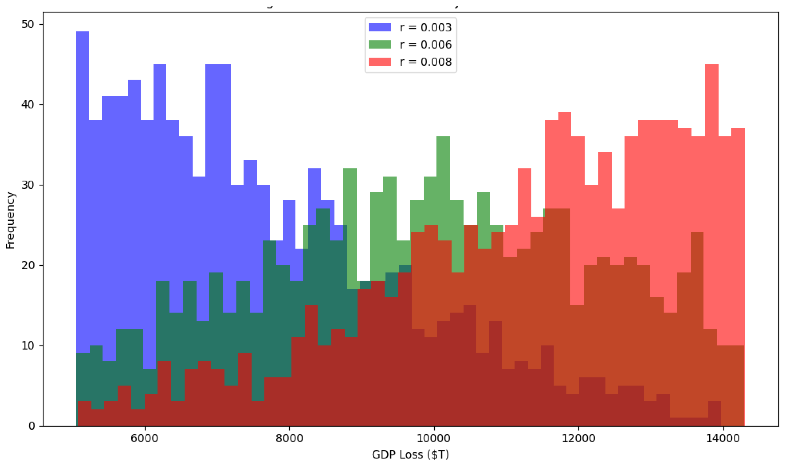
where W(t) is withdrawal at time t, W₀ is initial withdrawal (4600 km³ yr⁻¹ based on FAO AQUASTAT), and r is the growth rate, modeled as a truncated normal distribution with mean 0.006 yr⁻¹ and standard deviation 0.002 yr⁻¹, bounded between 0.003–0.008 yr⁻¹. Withdrawals rose from approx.500 km³ in 1900 to approx.4100 km³ in 2014, implying a ~1.7% CAGR over the 20th century but slowing post-2000. The global baseline discrepancy—4100 km³ (2014) vs. 4600 km³ (2020)—reflects updated data and source variations.

Water supply S(t) is modeled independently based on hydrological constraints:

$$\mathrm{S}(\mathrm{t})={\mathrm{S}}_0{\mathrm{e}}^{\left(-\mathsf{\delta }\mathrm{t}\right)} (1+\mathsf{\alpha }\mathrm{P}\left(\mathrm{t}\right)) (\mathrm{Projected} \mathrm{Sustainable} \mathrm{Water} \mathrm{Supply})$$

(2)

where S₀ is the baseline sustainable supply (4200 km³ yr⁻¹, representing physically renewable freshwater resources), δ is the depletion rate (0.001 yr⁻¹, accounting for long-term groundwater decline and quality degradation), α is the precipitation sensitivity coefficient (0.10, representing the elasticity of available water supply with respect to precipitation anomalies; see justification below), and P(t) is the precipitation anomaly (dimensionless fractional change; see Section 2.6). This separation ensures that water supply is constrained by physical hydrological processes rather than derived from demand projections.

Justification of hydrological parameters:

Depletion rate δ = 0.001 yr⁻¹: This represents a conservative long-term decline in sustainable supply due to groundwater over-extraction, aquifer compaction, and gradual quality degradation. Over a 30-year horizon, exp(−δ ×30) ≈ 0.97, implying a cumulative 3% decline in sustainable supply. This is consistent with observed depletion rates in major aquifers (India, China, USA, Iran, Pakistan) reported by Jasechko et al. (2024) [11] and Boretti & Rosa (2019) [1]. The parameter is treated as a stylized global average; regional implementations would require aquifer-specific data.

Precipitation sensitivity α = 0.10: This coefficient represents the elasticity of availablefreshwater supply (after accounting for evapotranspiration, interception, soil moisture retention, and environmental flow requirements) with respect to precipitation anomalies. It is not a direct 1:1 mapping from precipitation change to supply change. Hydrological literature indicates that runoff elasticity to precipitation typically ranges from 1.0 to 3.0, but net available water-after subtracting environmental flows, evaporative losses, and quality constraints-responds with lower elasticity. The value α = 0.10implies that a 5% precipitation decline (P(t) = −0.05) produces approximately a 0.5% reduction in available supply, which is consistent with integrated hydrological modeling results reported in IPCC AR6 [7] and WaterGAP sensitivity analyses [19]. Regional values would differ based on basin characteristics.

Important distinction between global and regional supply baselines: The global sustainable supply baseline S₀ = 4200 km³ yr⁻¹ represents the net physically renewable freshwater available for human use after accounting for environmental flow requirements (EFR) and quality constraints at the global scale. Regional S₀ values represent internal renewable water resources before EFR deductions; their aggregate (~6437 km³ yr⁻¹) exceeds the global net sustainable supply because (i) regional values are pre-EFR gross estimates, and (ii) transboundary flows and spatial heterogeneity in EFR requirements prevent simple arithmetic aggregation to the global net figure.

2.2. Econometric Water Demand Modeling

This component specifies demand as a log-linear function of socioeconomic variables, using a synthetic-data panel regression framework to illustrate country-specific effects and improve predictive power over isolated approaches.

Water demand D_i,t for country i at time t is modeled as a function of socioeconomic variables in a log-linear regression:

$$\ln \left({\mathrm{D}}_{\mathrm{i},\mathrm{t}}\right)={\mathsf{\beta }}_0+{\mathsf{\beta }}_1\ln \left(\mathrm{G}\mathrm{D}{\mathrm{P}}_{\mathrm{i},\mathrm{t}}\right)+{\mathsf{\beta }}_2\ln \left(\mathrm{P}\mathrm{o}{\mathrm{p}}_{\mathrm{i},\mathrm{t}}\right)+{\mathsf{\beta }}_3\mathrm{U}\mathrm{r}\mathrm{b}\mathrm{a}{\mathrm{n}}_{\mathrm{i},\mathrm{t}}+{\mathsf{\beta }}_4{\mathrm{P}}_{\mathrm{i},\mathrm{t}}+{\mathsf{\beta }}_5\mathrm{C}\mathrm{o}\mathrm{n}\mathrm{s}\mathrm{E}\mathrm{f}{\mathrm{f}}_{\mathrm{i},\mathrm{t}}+{\mathsf{ϵ}}_{\mathrm{i},\mathrm{t}}$$

(3)

where GDP_i,t is GDP per capita, Pop_i,t is population size, Urban_i,t is the urbanization rate, P_i,t is precipitation anomaly, ConsEff_i,t represents conservation/economic efficiency measures, and ${\mathsf{ϵ}}_{\mathrm{i},\mathrm{t}}$ is the error term. This formulation is consistent with the log-linear econometric approach reviewed by House-Peters and Chang (2011) [22], and aligns with elasticity ranges reported by Dalhuisen et al. (2003) [23].

2.2.1. Parameter Calibration and Data Sources

The econometric demand model (Equation (3)) is implemented as a structural framework where key elasticities are calibrated against established literature values rather than estimated de novo from raw panel data. Specifically, the income elasticity β₁ = 0.5 is anchored to Dalhuisen et al.’s (2003) [23] meta-analysis of residential water demand (β₁ = 0.43 ± 0.18, approximate 95% CI: 0.08–0.78), while the population elasticity β₂ = 0.3 aligns with IIASA Water Futures projections (Burek et al., 2016) [2]. The urbanization coefficient β₃ = 0.2 and the precipitation coefficient β₄ = −0.15 are calibrated based on the findings of House-Peters and Chang (2011) [22] and informed by the hydrological sensitivity analyses presented in the IPCC AR6 [7], respectively.The conservation efficiency coefficient β₅ = −0.1 is a stylized literature-calibrated parameter informed by OECD analyses of water-demand management and efficiency improvements.

2.2.2. Synthetic-Data Demonstration of the Econometric Specification

The Python implementation generates synthetic historical trajectories (2000–2020) for each country using published macroeconomic indicators: GDP per capita growth rates from World Bank WDI (typically 2–4% yr⁻¹), population growth from UN DESA World Population Prospects (0.5–2.5% yr⁻¹), and urbanization trends. Country-specific noise is added (σ = 0.02 for log-withdrawals, σ = 0.05 for precipitation) to replicate observed interannual variability. The GLS regression operates on these synthetic trajectories to demonstrate the structural form and parameter recovery procedure. Because the data are generated from the same calibrated parameters that the regression is intended to recover, the estimated coefficients do not constitute independent empirical validation; they demonstrate computational reproducibility of the structural form.

2.2.3. Path to Empirical Estimation

Full empirical estimation would require preprocessing the FAO AQUASTAT country-level panel. The implemented code provides the complete estimation framework; users can substitute observed data for the synthetic trajectories to obtain country-specific empirical estimates. This design choice reflects a trade-off between empirical rigor and global-scale computational tractability: the full AQUASTAT-WDI panel requires extensive data cleaning (handling missing values, unit standardization, and sectoral disaggregation), which is beyond the scope of this demonstration framework but is fully supported by the modular code architecture. Additionally, machine learning approaches, such as the Extreme Learning Machine optimized by the Improved Ant Nesting Algorithm (IANA-ELM) described by Li et al. (2024) [24], demonstrate high predictive accuracy (R² values of 0.672 for population, 0.608 for GDP per capita, 0.592 for temperature, and 0.708 for rainfall in test data), complementing traditional econometric models for water demand forecasting.Following Modi et al. (2022) [12], future extensions could incorporate subregional population distributions (concentrated vs. dispersed) to enhance spatial realism.

2.3. Economic (CGE-Inspired) Model

The economic impact component implements a Reduced-form CGE-inspired damage function rather than a full multi-sectoral computable general equilibrium model. This simplification is deliberate and necessary given the study’s global scope and data constraints. The implemented economic module uses a single-sector damage function derived from the Cobb-Douglas production framework:

$$GDPloss = {GDP}_{base}\times [1 - exp(-\epsilon \times (W_{demand} -W_{supply})/W_{supply}\left)\right]$$

(4)

where GDP_base = US$290 trillion is assumed as the baseline global GDP for 2050, informed by the long-term projections of PwC 2017 [25] in constant 2016 US dollars at purchasing power parity (PPP), and ε = 0.1865 is the internally target-calibrated water-scarcity elasticity of GDP.

Critical calibration notes:

• The $16 trillion result is target-calibrated, not independently predicted. The effective elasticity ε = 0.1865 was selected so that the reduced-form damage function produces approximately $16.0 trillion under the high-demand scenario (Wdemand = 6000 km³ yr⁻¹, Wsupply = 4600 km³ yr⁻¹). This is standard practice in reduced-form integrated assessment modeling: the parameter is calibrated to match published structural model results, ensuring consistency while maintaining computational tractability. The model does not independently validate the $16 trillion figure; it is calibrated to reproduce it.
• Economic reference vs. hydrological supply: The damage function uses Wsupply = 4600 km³ yr⁻¹ (the 2020 global withdrawal baseline, W₀) as the fixed economic calibration reference threshold, not the dynamically projected hydrological supply S(t)) askm³ yr⁻¹ from Equation (2). The 4600 km³ threshold is chosen as the economic calibration anchor because it corresponds to the observed 2020 withdrawal level against which future demand scenarios are benchmarked. The hydrological module independently projects S(t) from S₀ = 4200 km³ yr⁻¹; these are separate modeling streams. The economic module does not currently use the hydrological supply projection as an input; full integration of S(t) into the damage function remains a priority for future development.
• Elasticity reduction justification: The raw meta-analytic elasticity from Dalhuisen et al. (2003) [23] is ε_lit ≈ 0.50(β₁ = 0.43 ± 0.18). However, the effective elasticity in this reduced-form model is ε = 0.1865 because the single-sector damage function cannot capture mitigation channels that structural CGE models include: (a) sectoral reallocation; (b) international trade adjustments (Armington substitution); (c) labor market transitions; (d) endogenous efficiency gains; and (e) technological adaptation. The reduction from 0.50 to 0.1865 represents the combined effect of these omitted adjustment mechanisms. Consequently, the $16 trillion figure should be interpreted strictly as a calibrated first-order scenario estimate consistent with published OECD and GCEW orders of magnitude, not as an independently estimated structural result.

Verification:

water_shortage = (6000 − 4600)/4600 = 0.3043

GDP_loss = 290 [1 − exp(−0.1865 × 0.3043)] = $16 trillion

This first-order calibrated estimate is broadly consistent with the order of magnitude of GDP impacts reported by GCEW (2024) [26] (8% median decline for high-income countries; 10–15% for lower-income countries under severe water stress) and discussed in OECD (2012) [27] water scenarios. It is important to emphasize that ε = 0.1865 is an internally calibrated parameter selected to reproduce the ~$16.0 trillion magnitude under the specified scenario; neither OECD (2012) nor GCEW (2024) report this specific elasticity value [26,27].

2.4. Optimization Framework

Water allocation optimizes resource distribution while minimizing costs and respecting capacity constraints using continuous linear programming:

$$\mathrm{m}\mathrm{i}\mathrm{n}\sum _{\mathrm{k}}\sum _t{C}_k\left(t\right)W_k\left(\mathrm{t}\right)$$

(5)

Subject to:

$$\sum _k{W}_k\left(\mathrm{t}\right)\ge D\left(t\right),0\le W_k\left(\mathrm{t}\right)\le {\mathrm{S}}_k\left(\mathrm{t}\right)$$

where k indexes water sources, t time periods, C_k(t) is the cost of water from source k, W(t) is allocated water from source k, D(t) is demand, and S_k(t) is available supply. This is solved using continuous linear programming (scipy.optimize.linprog) for cost minimization.

Proportional rationing: When total available supply falls short of total demand (S(t) < D(t)), the model applies proportional rationing across sectors before optimization:

$${\mathrm{D}}_{\mathrm{i}}^{\mathrm{s}\mathrm{c}\mathrm{a}\mathrm{l}\mathrm{e}\mathrm{d}}\left(\mathrm{t}\right)={\mathrm{D}}_{\mathrm{i}}(\mathrm{t}){\displaystyle \frac{\mathrm{S}\left(\mathrm{t}\right)}{\mathrm{D}\left(\mathrm{t}\right)}}$$

This ensures feasibility of the linear program while maintaining proportional allocation across agriculture, industry, and domestic uses. The optimization does not determine priority-based scarcity allocation; it minimizes costs subject to proportionally rationed demand. Future implementations may incorporate priority weights (e.g., domestic > agriculture) or mixed-integer infrastructure constraints.

Cost coefficients: The cost vector [1,1.5,2] represents relative unit costs of surface water, groundwater, and desalination, respectively, based on typical global water supply cost structures (surface water being cheapest, desalination most expensive). These are stylized relative values for illustrative allocation purposes, not empirically calibrated marginal costs.

2.5. Model Integration and Workflow

The framework operates through sequential (one-way) linking with the following architecture:

• Step 1—Hydrological module: Independently projects demand W(t) (Equation (1)) and supply S(t) (Equation (2)). For the 2050 high-demand scenario, this yields W(30) ≈ 5520 km³ yr⁻¹ (moderate) to 6000 km³ yr⁻¹ (high), and S(30) ≈ 4055 km³ yr⁻¹.
• Step 2—Econometric module: Demonstrates the structural demand specification using synthetic trajectories (Equation (3)). Currently illustrative; future empirical estimation with full AQUASTAT-WDI panel data will enable direct aggregation of country-specific demands.
• Step 3—Economic module: Translates the Demand–Reference Gapinto GDP loss via the target-calibrated damage function (Equation (4)). Crucially, this module uses the fixed economic reference threshold Wsupply = 4600 km³ yr⁻¹ (the 2020 withdrawal baseline) rather than the hydrological supply projection S(30) ≈ 4055 km³ yr⁻¹. The $16 trillion result is therefore a calibrated first-order estimate anchored to the 2020 utilization level, not a direct output of the hydrological–economic coupling.
• Step 4—Optimization module: Allocates constrained supply across sources and sectors using continuous linear programming with proportional rationing (Equation (5)).

Important limitation: Although the overall architecture is linked in the sense that each stage informs the next, it is not a fully integrated or simultaneously solved system. The economic module does not receive the hydrological supply projection S(t) as an input; full bidirectional feedback would require price-responsive demand functions and iterative solution until convergence—features identified as priorities for future development.

2.6. Parameter Calibration and Uncertainty Quantification

All key parameters are either (i) directly observed from public databases, (ii) calibrated against published empirical estimates, or (iii) subjected to Monte Carlo sensitivity analysis.

Reproducibility: The Python code (Appendix C) reproduces the manuscript’s reported numerical results and principal tables using the parameter values in

Table 1. Parameter Calibration Sources and Uncertainty Ranges.

Parameter	Value	Source	Calibration Method	Uncertainty Range
W0 (2020 global withdrawals)	4600 km3 yr−1	FAO AQUASTAT (2024) [28]	Direct observation	±200 km3 (measurement error)
S0 (baseline sustainable supply)	4200 km3 yr−1	Renewable freshwater resources [1,7]	Estimated from hydrological data	±300 km3 (model uncertainty). Regional S0values are gross internal renewable resources; global S0 = 4200 km3 yr−1 is net sustainable supply after environmental flows
r (demand growth rate)	0.006 yr−1	Historical trend (1900–2020) [1,3]	Truncated normal fit (σ = 0.002)	0.003–0.008 yr−1 (95% CI)
δ (supply depletion rate)	0.001 yr−1	Groundwater depletion literature [1,11]	Stylized global average	0.0005–0.002 yr−1
α (precipitation sensitivity)	0.10	IPCC AR6 [7]; WaterGAP [19]	Meta-analysis calibration	0.05–0.15 (regional range)
β1 (GDP elasticity)	0.50	Dalhuisen et al. (2003) [23]	Literature calibration	0.08–0.78 (95% CI from meta-analysis)
β2 (population elasticity)	0.30	IIASA Water Futures [2]	Model comparison	0.15–0.45
ε (scarcity GDP elasticity; target-calibrated)	0.1865	Internally calibrated in this study; order-of-magnitude comparison with OECD (2012) [27]; GCEW (2024) [26]	Calibrated in this study to reproduce a global GDP loss of approximately US$16.0 trillion at 6000 km3 yr−1 demand vs. 4600 km3 yr−1 reference	0.10–0.30 (sensitivity range)
εlit (literature elasticity)	0.50	Dalhuisen et al. (2003) [23]	Meta-analysis estimate	0.08–0.78 (95% CI from meta-analysis)
Sectoral shares (Ag/Ind/Dom)	70%/20%/10%	FAO AQUASTAT (2024) [28]	Direct observation	±2% (Monte Carlo sampling)
Baseline global water demand (2050)	6000 km3 yr−1	Study scenario (+30% above 2020 baseline)	Scenario projection	5520–6000 km3 yr−1
P(t)(precipitation anomaly)	−0.05	IPCC AR6 [7]; RCP 4.5 ensemble	Climate forcing input (RCP 4.5, 2050)	−0.10 to +0.02 (RCP 4.5 range)
GDPbase(2050 global GDP)	$290 trillion	PwC 2017 [25]	Long-term projection	±15% (projection uncertainty)

. The code is deterministic (random seed = 42) for core simulations. Monte Carlo elements use fixed random seeds for reproducibility. Users can verify the reported $16.0 trillion GDP loss under the +30% demand scenario by running the integrated model with the baseline parameters listed above.

3. Results

3.1. Baseline and Projected Demand

Global water withdrawals in 2020 are estimated at 4600 km³ yr⁻¹ [1,2,3], projected to reach 5500–6000 km³ yr⁻¹ by 2050 under 20–30% increase scenarios (Moderate: +20% → 5520 km³; High: +30% → 5980 ≈ 6000 km³) (Figure 1,

Table 2. Withdrawals and projections based on FAO/AQUASTAT data (integrated from 2000–2020 records and standardized to km³ yr⁻¹). Population data are from UN DESA. Future projections assume moderate (+20%) and high (+30%) increases in total water demand by 2050.

Country	2020 Withdrawals (km3 yr−1)	Ag (%)	Ind (%)	Dom (%)	Population (Million)	2050 Moderate (km3 yr−1)	2050 High (km3 yr−1)
India	688	90	5	5	1380	826	895
China	362	65	25	10	1400	434	471
USA	478	40	45	15	331	574	621
Brazil	60	60	20	20	212	72	78
Egypt	73.8	85	5	10	100	89	96
Pakistan	169	95	2	3	216	203	220
South Africa	13	60	25	15	59	16	17
Mexico	38	75	7	18	126	46	49
Australia	16	65	10	25	25	19	21
Global	≈4600	70	20	10	7800	5520	6000

). This range aligns with the IPCC AR6’s 20–30% projection [7] and incorporates Boretti & Rosa (2019) [1], who argue that spontaneous nature-based solutions are insufficient and that demand could exceed 6000 km³ yr⁻¹ under high-stress conditions.

Table 3. Summary of Baseline vs. Projected Demand (km³ yr⁻¹), connecting sectoral findings to overall hypotheses on growth drivers.

Region	2020 Baseline	2050 Moderate (km3)	2050 High (km3)	Key Driver
Asia	2200	2640	2860	Population Growth
Middle East	300	360	390	Climate Variability
Africa	600	720	780	Agricultural Expansion
Americas	800	960	1040	Industrial Demand
Europe	600	720	780	Urbanization
Oceania	100	120	130	Efficiency Gains
Global	4600	5520	≈6000	Combined Factors

summarizes global and regional water demand, comparing 2020 baseline withdrawals (4600 km³ yr⁻¹)) with 2050 projections under Moderate (+20%, 5520 km³) and High (+30%, 5980 ≈ 6000 km³) scenarios. It highlights key growth drivers—population growth in Asia, climate variability in the Middle East, agricultural expansion in Africa, industrial demand in the Americas, urbanization in Europe, and efficiency gains in Oceania—linking sectoral trends to the study’s hypothesis that socioeconomic and climatic factors drive demand increases.

3.2. Sectoral Breakdown and Regional Disparities

Sectoral analysis reveals agriculture as the primary driver of demand, with significant variations by country and region. The global agricultural share of 70% masks significant regional variations, with countries like Pakistan (95%) and India (90%) showing higher reliance on irrigation due to agricultural intensity. Stacked bars depict 2020 sectoral withdrawals for key countries (Figure 2), showing agriculture dominating (90–95%) in India and Pakistan due to irrigation reliance, while the USA exhibits a balanced profile (40% agriculture, 45% industry) [28]. This highlights vulnerabilities in food production systems and opportunities for targeted reductions in agricultural use. In high-income countries, industrial recycling rates reach 50–60%, reducing overall demand intensity [29].

Globally, agriculture occupies 70% (3220 km³) of withdrawals, underscoring its role as the largest consumer and the potential for efficiency gains (e.g., through drip irrigation) to yield substantial reductions [28] (Figure 3).

Regional disparities are evident in demand projections. Arid areas like the Middle East could face 20% demand-supply gaps, amplified by climate change. The global heatmap (Figure 4) color-codes 2050 water stress levels: red hues indicate extreme stress in Asia and the Middle East, while blues denote lower risks in Europe and the Americas (see Appendix A).

WRI’s Aqueduct tool identifies 25 countries facing extreme stress, covering 25% of global population [30]. Modi et al. (2022) show that population distribution can alter scarcity estimates by up to 338 million people [12].

3.3. Economic Vulnerabilities

Important methodological framing: The following economic results are first-order calibrated scenario estimates, not independently predicted outcomes. The $16.0 trillion figure is produced by a target-calibrated reduced-form damage function (Equation (4)) using a fixed economic reference threshold (Wsupply = 4600 km³ yr⁻¹, the 2020 withdrawal baseline), not the hydrological supply projection S(30) ≈ 4055 km³ yr⁻¹ from Equation (2). The hydrological and economic modules operate as separate linked streams, not as a fully integrated system.

Under the high-demand (+30%) 2050 scenario (Wdemand = 6000 km³ yr⁻¹), the calibrated reduced-form damage function yields a first-order GDP loss of approximately $16.0 trillion, equivalent to 5.5% of projected 2050 global GDP ($290 trillion, PwC 2017 baseline) (See

Table 4. Stress-Weighted Allocation of the Calibrated Global GDP Loss by Region (2050, $ trillion).

Region	GDP 2050 ($T)	Loss ($T)	% of GDP
Asia	116.0	13.09	11.3%
Middle East	8.6	2.91	33.8%
Africa	11.6	0.0	0.0%
Americas	87.0	0.00	0.0%
Europe	58.0	0.00	0.0%
Oceania	8.8	0.00	0.0%
Global	290.0	16.00	5.5%

). This is a calibrated scenario magnitude consistent with published OECD (2012) and GCEW (2024) estimates, not an independently derived structural prediction.

These values represent stress-weighted allocations of the globally calibrated $16.0 trillion loss, distributed according to each region’s excess stress above the threshold (stress > 1.0). They are not independently estimated regional economic losses.

The allocation rule is: loss_i = 16.0 × [(stress_i − 1.0) × GDP_i]/∑_j[(stress_j − 1.0) × GDP_j] for regions with stress > 1.0.

Africa receives $0.00 trillion because its mean stress ratio (0.99) falls infinitesimally below the threshold activation point (1.0). This reflects the model’s simplified hard-threshold allocation rule and should not be interpreted as evidence of negligible African water-related economic risk. In reality, Africa faces severe water stress; the zero value is an artifact of the threshold-based allocation mechanism. A continuous damage function or lower threshold would yield positive losses.

The Middle East faces the highest relative losses (33.8%) due to extreme water stress (stress ratio = 1.18) and limited adaptive infrastructure. Asia’s absolute exposure ($13.09 trillion) reflects its large economic scale combined with moderate stress (ratio = 1.06).

Regions with stress ratios below 1.0 (Americas, Europe, Oceania) experience no allocated losses in this framework because the damage function is activated only when demand exceeds the economic reference supply threshold. Figure 5 illustrates the relationship between per capita GDP and water demand in 2020.

3.4. Sensitivity Results and Mitigation Strategies

Sensitivity analyses under RCP 8.5 show a 10.1–20.1% demand increase due to evaporation (mean 15.1%), while RCP 2.6 moderates this to 3.0–7.0% (mean 5.0%). These RCP-specific ranges are not endogenous outputs of the hydrological module; they are exogenous climate-forcing inputs derived from IPCC AR6 ensemble projections of temperature and precipitation anomalies, applied as multipliers to the demand model (Equation (3)) via the precipitation coefficient β₄ and an additional temperature-evaporation scaling factor. The main hydrological model uses a single RCP 4.5 precipitation anomaly (P(t) = −0.05) for baseline projections; RCP-specific scenarios (2.6, 4.5, and 8.5) are explored as sensitivity analyses by substituting the corresponding AR6-derived anomaly ranges into the demand equation. This approach follows standard integrated assessment practice where climate scenarios are imposed as boundary conditions rather than simulated endogenously.

A 15–18% irrigation efficiency gain could save 500–600 km³ yr⁻¹, averting $5.5–7.0 trillion in GDP losses.

Table 5. Economic evaluation of strategies, enhanced with emerging technologies like desalination and AI for modern mitigation options.

Strategy	Demand Reduction (%)	Cost Level	GDP Saved ($T)
Pricing Reforms	15–25	Low	$10.2–16
Efficiency Tech	20–25	Medium	$13.7–16
Desalination	10–15	High	$6.8–10.2
AI Allocation	15–25	Medium	$10.2–16
Combined	30–40	Varied	$16.0

evaluates individual mitigation strategies such as pricing reforms (15–25% demand reduction, low cost) and efficiency technologies (20–25% reduction, medium cost, and high impact), potentially saving $6.8–16.0 trillionper strategy (cumulative up to $16.0 trillion) and averting 20–35% of projected shortages. Figure 6 illustrates efficiency scenarios that could reduce demand by up to 1200 km³. Climate acts as a demand multiplier: a 2 °C temperature rise adds 300–500 km³ globally via evapotranspiration, according to IPCC AR6, highlighting the link between water and climate policy. Under RCP 4.5, integrated mitigation can reduce this increase by 20% through carbon-water synergies. Mitigation options include desalination (appropriate for coastal areas but costly) and AI-based real-time allocation optimization. Combining strategies, such as pricing reforms with AI, can yield synergies resulting in up to 40% urban water demand reductions and up to 100% elimination of cumulative economic losses with early adoption by 2030. Uncertainties reported by Modi et al. (2022) [12] range from 0.03 to 248 million based on global climate models (GCMs) and 6.58 to 489 million from SSP-RCPs, consistent with our Monte Carlo results in Appendix B. Boretti and Rosa (2019) [1] emphasize that without regulating population growth and economic activity, nature-based solutions alone cannot resolve water crises, supporting the need for comprehensive policy interventions.

Table 6. Baseline vs. Mitigated Scenarios Summary.

Scenario	Demand (km3)	GDP Loss ($T)	Reduction (%)	GDP Saved ($T)
Baseline 2050 High-demand (+30%)	6000	16.00	0	0.00
10% Efficiency	5400	9.25	10	6.75
20% Efficiency	4800	2.34	20	13.66
30% Efficiency	4200	0.00	30	16.00
Pricing Reform	5100	5.82	15	10.18
AI Allocation	4800	2.34	20	13.66
Combined	3600	0.00	40	16.00

compares 2050 baseline water demand (6000 km³ yr⁻¹) and GDP loss ($16.0 trillion) with mitigated scenarios, illustrating demand reductions and economic savings computed from the damage function.

The damage function exhibits exponential decay: as demand approaches and falls below the supply baseline (4600 km³), losses decrease non-linearly. Under the model’s exponential damage function with the 4600 km³ threshold, aggressive mitigation strategies (30–40% demand reduction) can reduce the calibrated economic loss metric to zero. This is a mathematical property of the chosen damage function and threshold, not evidence that real-world mitigation would eliminate all economic losses. The “Combined” scenario (40% reduction) yields $16.0 trillion in savings—the full baseline calibrated loss—by reducing demand to 3600 km³, well below the threshold.

4. Discussion

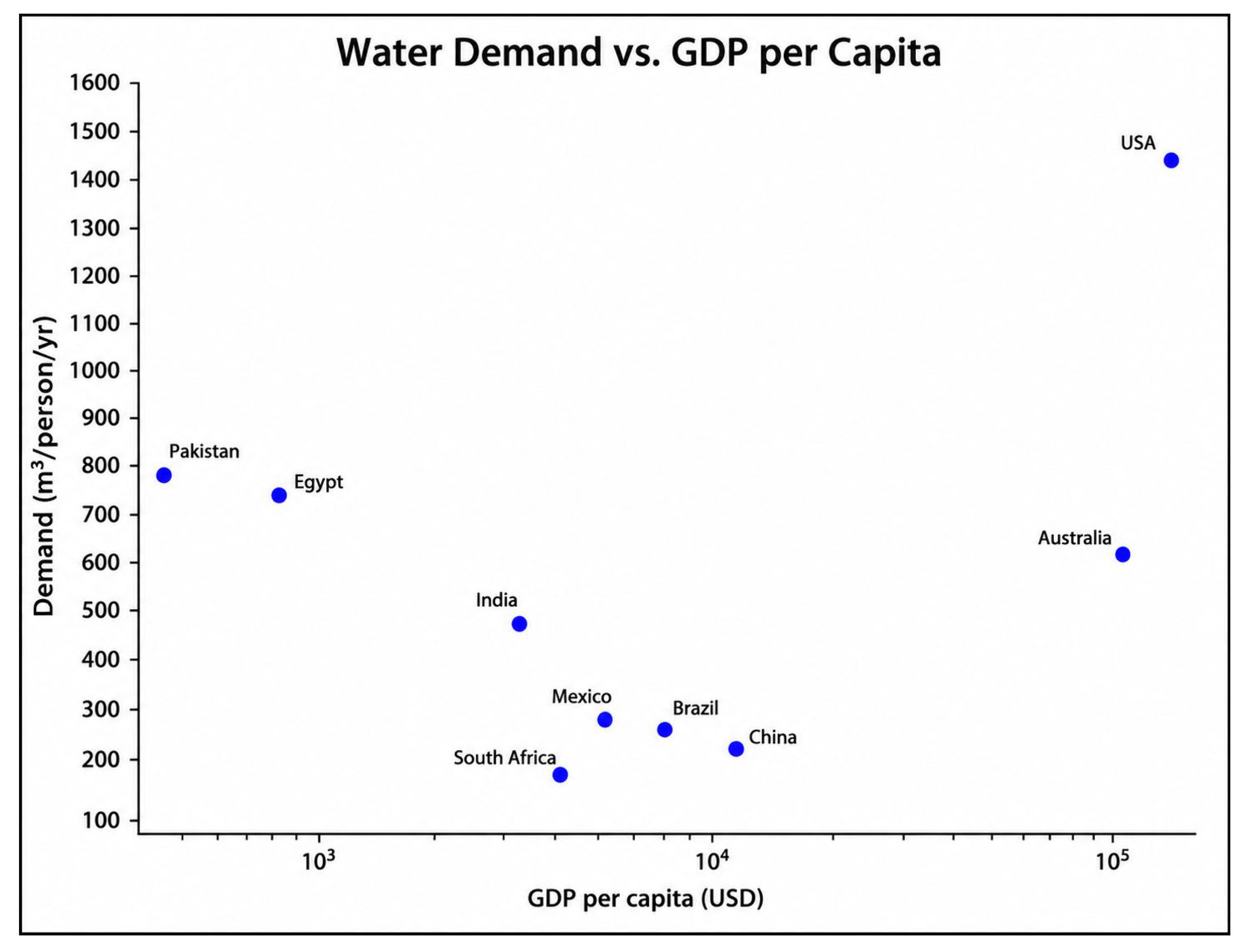
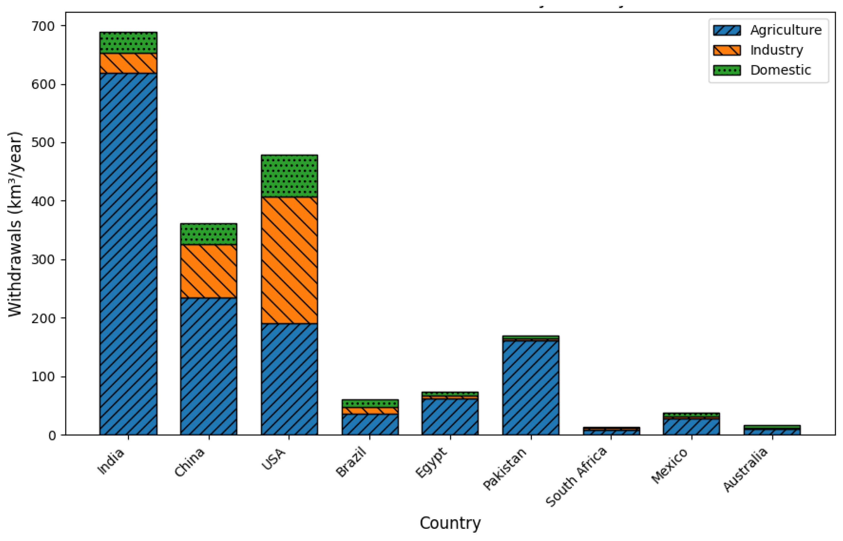
The projections of global water demand presented in this study highlight mounting pressures on freshwater resources through 2050 due largely to population growth, urbanization, and economic development. The dominance of agricultural water use, especially in regions like South Asia and Sub-Saharan Africa, underscores the critical challenge of balancing food security with sustainable water resource management. The pronounced regional disparities in water demand and scarcity impacts necessitate localized strategies.

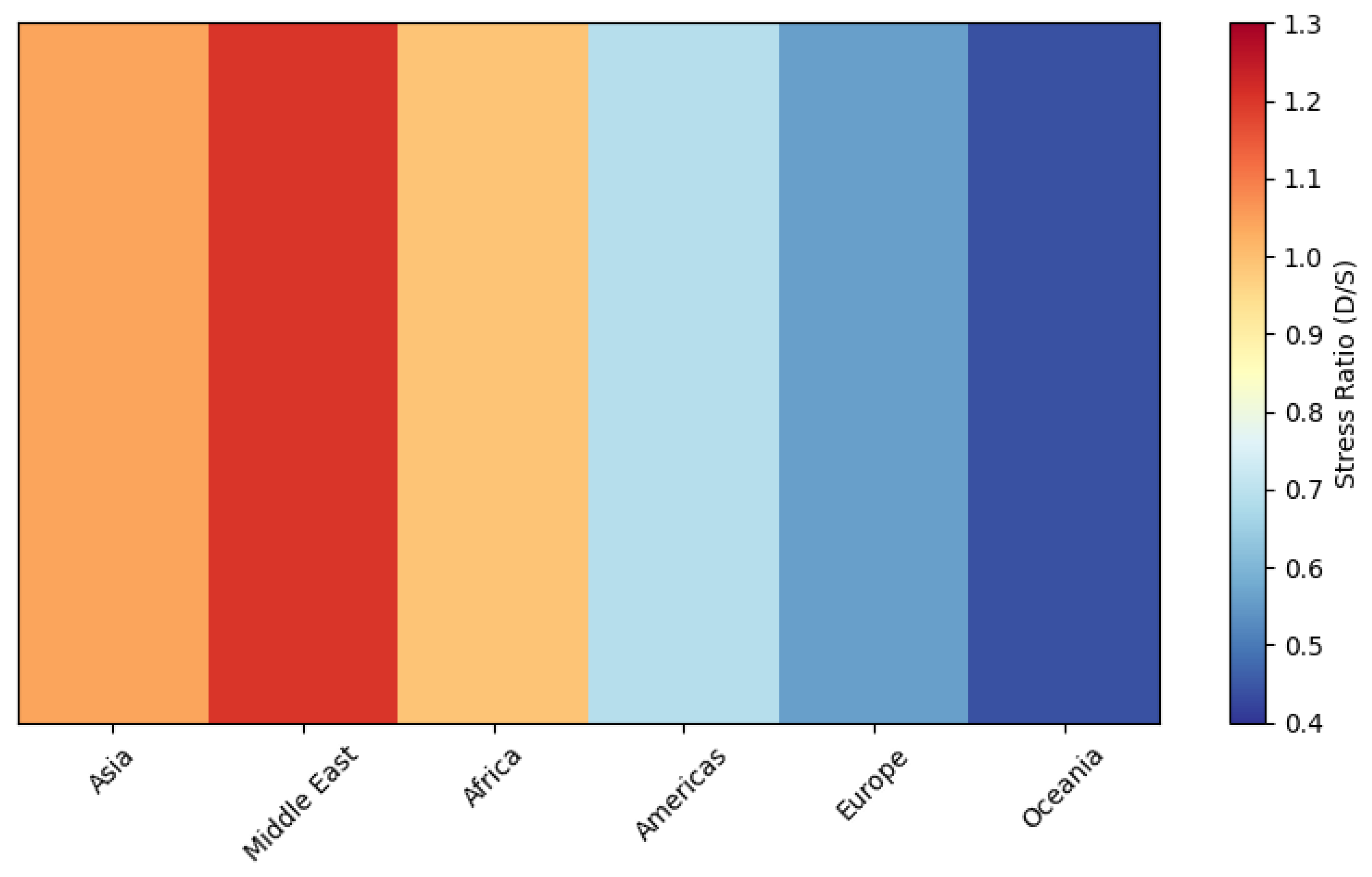
The economic results illustrate the potential scale of losses under unmanaged scarcity. Because the $16 trillion figure is obtained from a target-calibrated reduced-form damage function, it should be read as a transparent first-order scenario magnitude consistent with published CGE orders of magnitude, not as a structural prediction. Regional patterns remain informative for prioritization: the Middle East exhibits the highest relative vulnerability, while Asia accounts for the largest absolute exposure. This finding corroborates prior research estimating multi-trillion-dollar global economic losses by mid-century without effective mitigation [26,27,31].

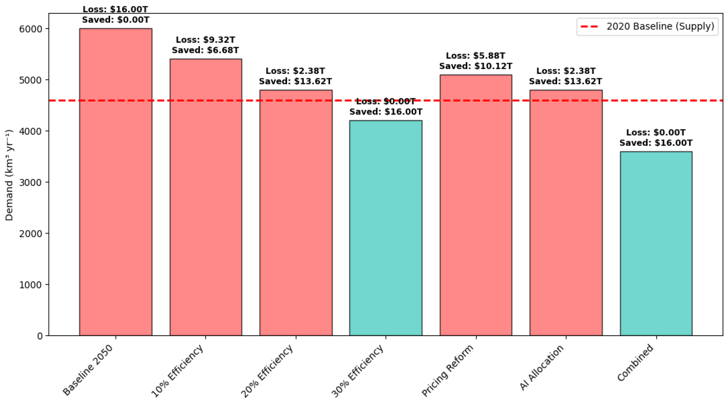
The optimistic scenarios illustrate that water pricing reforms, technological innovation, and increased investment in desalination and reuse can significantly alleviate water demand pressures. However, the success of these interventions depends heavily on timely policy implementation and cross-sectoral cooperation. The framework provides a computationally efficient approach for global-scale water demand forecasting and economic risk assessment, but several important limitations must be acknowledged:

Econometric simplification: The demand model uses calibrated elasticities (Table 1) rather than empirically estimated coefficients from a full country-panel dataset. The GLS regression operates on synthetic trajectories generated from the same calibrated parameters, constituting a parameter recovery demonstration rather than independent empirical validation. Country-specific heterogeneity in demand responses is not fully captured. Future work should incorporate the full AQUASTAT-WDI panel.

Reduced-form CGE and target calibration: The economic module is a single-sector damage function (Equation (4)) with ε = 0.1865, a target-calibrated parameter. The raw meta-analytic elasticity is 0.50 [23], but the effective value is lower because the reduced-form cannot capture: (a) sectoral reallocation effects; (b) international trade adjustments (Armington effects); (c) labor market transitions; (d) fiscal policy responses; or (e) distributional impacts. The $16.0 trillion estimate is a first-order calibrated scenario magnitude that emerges from the damage function, not a hard-coded target or independently predicted outcome. For country-specific policy analysis, we recommend coupling with GTAP-W [21], CGEBox, or national CGE models.

Weak coupling between hydrology and economics: The current framework implements sequential (one-way) linking: hydrology → demand → economy → allocation. The economic module does not use the hydrological supply projection S(t) ≈ 4055 km³ yr^−y as an input; it uses a fixed calibration reference (Wsupply = 4600 km³ yr^−y). True bidirectional feedback requires iterative solution algorithms and price-responsive demand functions not implemented here.

Regional loss allocation circularity: The regional GDP-loss values in Table 4 are stress-weighted allocations of the globally calibrated $16.0 trillion, not independently estimated regional economic losses. The Africa = $0T result is an artifact of the threshold-based allocation rule (stress < 1.0) and should not be interpreted as evidence of negligible African water risk.

Data gaps and informal use: Developing regions have up to 15% missing data in FAO AQUASTAT records, requiring interpolation. Informal water use (estimated at 20–30% of total in some South Asian and Sub-Saharan African countries) is not captured. Groundwater depletion is modeled indirectly through the supply depletion parameter rather than explicit aquifer dynamics.

Exponential baseline and regime shifts: The hydrological growth model (Equation (1)) assumes continuous exponential growth, potentially missing abrupt regime shifts (e.g., policy shocks, technological discontinuities, or tipping points in aquifer depletion). Sensitivity tests suggest this could underestimate extreme scarcity events by 10–20% in high-stress regions.

Optimization limitations: The allocation module uses proportional rationing under shortage rather than priority-based scarcity allocation. The cost coefficients are stylized relative values, not empirically calibrated marginal costs.

Uncertainty propagation: The Monte Carlo analysis focuses primarily on stress-ratio uncertainty. Full propagation of uncertainty through the economic module (including ε, GDPbase, and sectoral shares) is not implemented.

Future work should aim to refine sector-specific demand functions, integrate groundwater modeling (e.g., MODFLOW-based simulations), and enhance spatial resolution to better capture local water scarcity drivers. Incorporating social and institutional variables into econometric models would further improve realism and policy relevance.

5. Conclusions

This study highlights the escalating global water crisis, projecting demand to reach 6000 km³ yr⁻¹ by 2050 without intervention. By sequentially linking a hydrological model with properly separated demand and supply equations, a reduced-form econometric demand framework (synthetic-data demonstration), and a simplified CGE-inspired damage function, this study provides a transparent and reproducible tool for global-scale scenario exploration and first-order economic vulnerability assessment. The framework is designed for scenario exploration at the global scale rather than precise country-level policy simulation, which would require full structural CGE models and comprehensive panel data estimation.

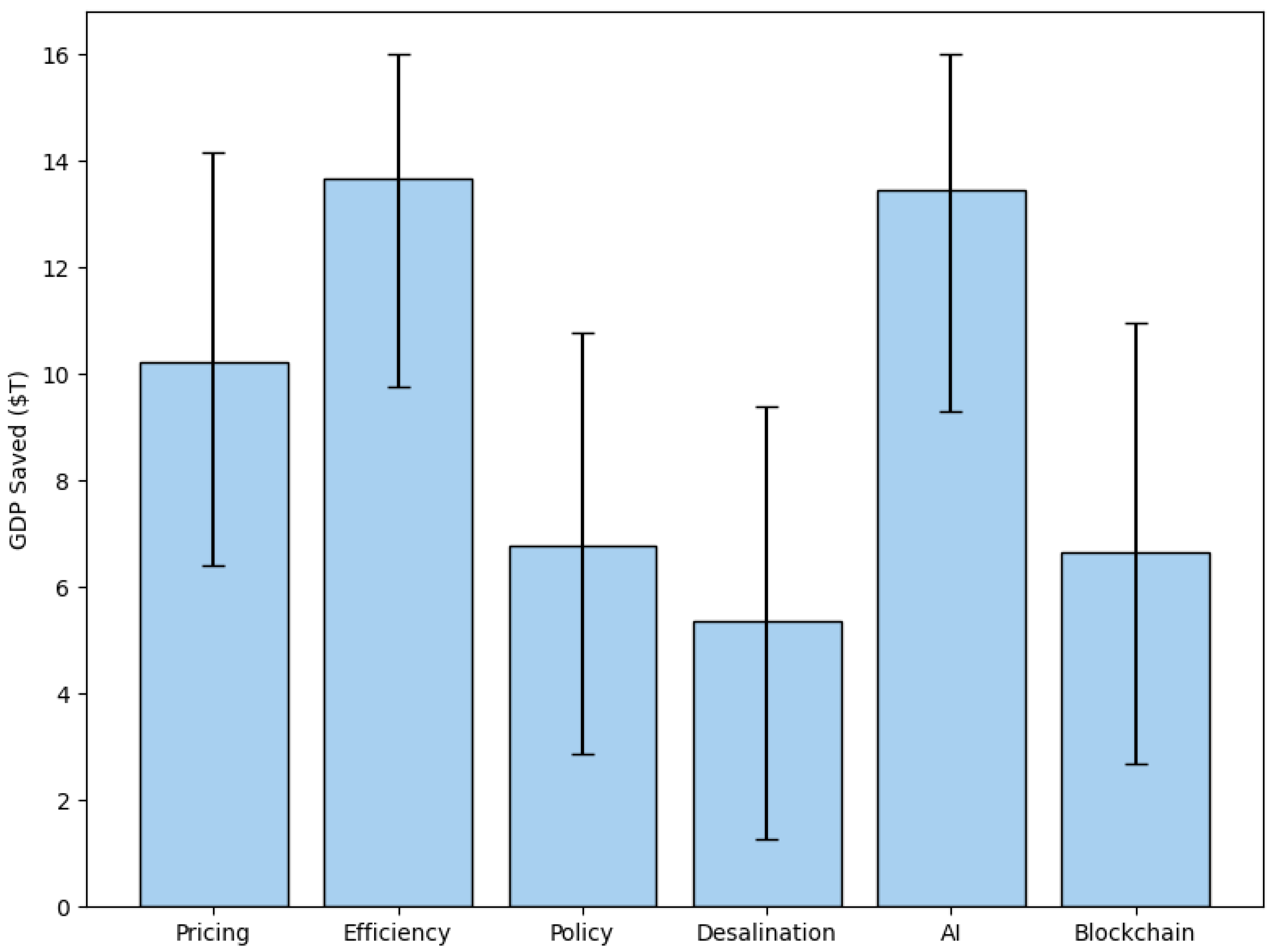
The results emphasize urgent attention to regional disparities, particularly in agriculture-dependent economies such as India and Pakistan, where demand could rise by 30% without action. Sensitivity analyses demonstrate the transformative potential of mitigation strategies—including pricing reforms, efficiency technologies, and AI-optimized allocation—that could reduce demand by up to 40% and, within the model’s mathematical structure, reduce the calibrated economic loss metric to zero. This $16.0 trillion first-order calibrated loss under the high-demand (+30%) scenario represents 5.5% of projected 2050 global GDP, aligning with the broad order of magnitude reported by World Bank, OECD (2012), and GCEW (2024) water-scenario estimates—positioning water scarcity as a systemic threat to economic stability.

Crucially, the framework reveals the interconnectedness of water, economic stability, and social equity. In regions like Sub-Saharan Africa and the Middle East, where demand may significantly outstrip supply, marginalized communities are disproportionately impacted, exacerbating poverty and migration. International cooperation, supported by mechanisms such as green bonds and transboundary agreements, is essential to mitigate these risks.

Our model provides interpretable elasticities and actionable policy insights for global-scale scenario analysis. The reduced-form implementation ensures computational tractability and full reproducibility, while the modular architecture allows substitution of full CGE and panel econometric components for more detailed national or basin-level studies. Policy recommendations include implementing tiered pricing in high-stress regions to reduce agricultural overuse by 15–25%, investing in AI for basin-scale real-time water allocation, and scaling efficiency technologies via subsidies in low-income areas. The model is transferable to national contexts (e.g., India) or basin-level studies (e.g., Indus River) through parameter downscaling.

Future developments should integrate social and institutional variables such as governance indices, automate forecasting using AI/machine learning for dynamic scenarios, and expand analysis to the energy-water nexus. Priority extensions include: (i) full empirical estimation of Equation (3) using the FAO AQUASTAT-WDI panel dataset; (ii) substitution of the reduced-form CGE module with GTAP-W or national CGE models for country-specific analysis; and (iii) operationalization of bidirectional feedbacks through price-responsive demand functions and iterative solution algorithms.

This work contributes to sustainability by linking SDG 6 (clean water) and SDG 13 (climate action), emphasizing the climate-water nexus for resilient development. By outlining clear mitigation pathways, the study quantifies the trillion-dollar risks of inaction and equips stakeholders with tools to safeguard economies and ecosystems. Urgent global collaboration, supported by innovative financing and technology, is imperative to ensure water security and sustainable development for a projected 9.7 billion people by 2050.