A Coupled Simulation and Flood Mitigation Design Framework for Urban Waterlogging Based on LID Spatial Layout Optimization

Abstract

Urban stormwater poses a threat to urban safety and development. The systematic spatial planning of low-impact development (LID) facilities is increasingly recognized as a sustainable approach to enhancing urban flood resilience. Previous studies have largely focused on empirically-based design approaches or have employed uncoupled computational methods, resulting in a lack of accuracy in flood simulation results. In this study, a novel framework was proposed. The Non-dominated Sorting Genetic Algorithm II was employed to perform multi-objective optimization of the spatial layout of LID facilities, and a coupled model of SWMM and TELEMAC was developed to simulate surface flooding based on the optimized schemes. Under three rainfall scenarios, three schemes on the Pareto Front—representing the lowest cost, the optimal compromise and the least overflow—were selected to investigate how scheme parameters and overflow are influenced by rainfall intensity and design preferences. The results indicate that scheme parameters and node overflow show greater variation under the influence of different design preferences than under different rainfall conditions. Taking the schemes selected in this study as examples, under the lowest-cost scheme, LID coverage was less than 10%, resulting in a limited reduction in node overflow; but when ‘minimum overflow’ was set as the design preference, node overflow was virtually eliminated, with peak water levels at flood-prone locations reduced to 0.05 m, 0.08 m and 0.10 m under 50-year, 100-year and 200-year storm conditions, respectively. The framework for urban flooding simulation and flood control scheme design proposed in this study is potentially applicable to comparable settings, subject to similar data availability and physical conditions, serving as a reference for enhancing urban resilience to flooding.

1. Introduction

Urban flooding is currently one of the most severe natural hazards confronting human society, inflicting substantial damage on urban areas annually [1], and the threat is escalating year by year. Global climate change has increased both the frequency and intensity of extreme rainfall events, while accelerated urbanization has dramatically expanded impervious surface coverage in urban areas, thereby disrupting the natural hydrological cycle [2]. At present, cities are commonly characterized by aging drainage networks, insufficient stormwater harvesting facilities, and low green-space coverage, all of which compromise urban resilience to rainstorms. Consequently, stormwater runoff cannot be discharged in a timely manner, and flood disasters occur frequently [3,4]. In July 2021, an extraordinary rainstorm struck Zhengzhou, claiming 380 lives and causing direct economic losses of up to 40.9 billion CNY [5]. In July 2023, North China was hit by severe floods, debris flows, and urban waterlogging, affecting approximately one million people [6,7]. Effectively coping with the ever-growing threat of urban stormwater flooding has thus become a central challenge constraining the sustainable development of urban areas.

To date, scholars at home and abroad have primarily focused on simulating the formation and concentration processes of rainstorm-induced urban floods to assess regional flood risks and to propose corresponding mitigation measures [8]. In recent years, research has gradually shifted from simulating drainage performance based on grey infrastructure alone toward integrated low-impact development (LID) management frameworks that incorporate green infrastructure [9]. In 1971, the Storm Water Management Model (SWMM, version 5.2, U.S. Environmental Protection Agency, USA) was developed by the U.S. Environmental Protection Agency, mainly to simulate urban underground pipe networks and to deploy individual LID measures or LID combinations within designated areas [10]. Most LID layouts are determined empirically. Taking an urban community as the study area, Jiang et al. [11] employed SWMM to construct four scenarios—conventional drainage, single LID, storage tank, and combined LID–storage tank—and compared the runoff and discharge processes of each scheme under six return periods ranging from 1 to 50 years. The results demonstrated that the combined LID–storage tank scheme could stably reduce peak site discharge and alleviate the pressure on municipal pipe networks, outperforming any single measure. However, empirically based LID placement cannot account for all relevant factors [12]. Node overflow within drainage networks is governed by multiple interacting factors, and empirical judgment alone tends to result in redundant LID deployment in certain areas while leaving critical convergence nodes under-equipped [13]. Moreover, different LID types exhibit distinct runoff-reduction characteristics, and empirical decision-making struggles to achieve collaborative optimization under multi-objective constraints. Various algorithms have therefore been introduced to optimize LID placement. Li et al. [14] were among the first to couple an improved non-dominated sorting particle swarm optimization (NSPSO) algorithm with SWMM, taking minimization of engineering cost and flooding risk as objectives, to establish a multi-objective optimization framework for urban stormwater storage tank design. Building on this framework, Duan et al. [15] further incorporated LID facilities as decision variables and applied an improved particle swarm algorithm (NPSO) to obtain the Pareto optimal set for the joint deployment of storage tanks and LIDs. Their results showed that incorporating LIDs significantly reduced both system cost and flood risk simultaneously. More recently, the Non-dominated Sorting Genetic Algorithm II (NSGA-II), owing to its favorable convergence performance, uniform solution distribution, and strong adaptability to discrete variables in multi-objective optimization, has been increasingly applied to LID layout optimization. Addressing the dual problems of urban waterlogging and non-point source pollution, Li Jinlin [16] employed an LSTM + DNN model for rainfall prediction, adopted an ISSA-BP algorithm for the intelligent calibration of SWMM parameters, and applied NSGA-II to optimize LID configuration schemes, thereby enhancing stormwater management efficiency and providing new insights for subsequent decision-making.

SWMM possesses well-established rainfall–runoff and pipe-network hydrodynamic simulation modules, and performs excellently in representing one-dimensional hydrodynamic processes [17]. However, SWMM lacks a two-dimensional hydrodynamic module, which limits its ability to accurately compute surface inundation depth and runoff velocity, and consequently constrains its capability to describe overland flow processes. TELEMAC-2D (version v8p4, National Hydraulics and Environment Laboratory of France, France), by contrast, has demonstrated strong performance in simulating two-dimensional overland flow and has been widely applied by researchers to studies of rivers and lakes, estuarine and coastal regions, and urban flooding [18]. A coupled model integrates the two, enabling whole-process simulation of rainfall–runoff, pipe-network flow, and two-dimensional surface inundation [19]. Coupling the optimized 1D pipe-network results with a 2D surface model can therefore more intuitively reveal the surface-level effectiveness of optimized schemes, providing a basis for subsequent urban renewal. Currently, the two-dimensional hydrodynamic models widely used for urban stormwater simulation include platforms and software such as LISFLOOD-FP, WCA-2D, the MIKE series, and TELEMAC. With respect to coupled models, Wang Zhaoli et al. [20] developed a novel coupled model, TSWM, based on SWMM and TELEMAC-2D, evaluated its applicability and reliability through historical rainstorm validation and model comparison, and conducted numerical simulations under rainstorms of different return periods. Ye Chenlei et al. [21] constructed a street-block-scale urban flood simulation model by coupling SWMM with InfoWorks ICM, simulated the distribution of surface inundation and hazard under various rainfall scenarios, and comparatively evaluated the reliability of the simulation results.

Despite these advances, a clear research gap remains. Most existing studies fail to integrate multi-objective low-impact development (LID) optimization with high-resolution 2D surface inundation modeling. Specifically, research on LID layout optimization often relies solely on 1D drainage models (e.g., SWMM). Conversely, studies using coupled 1D-2D hydrodynamic models rarely employ optimization algorithms for systematic LID placement, relying instead on empirical designs.

To address this, this paper proposes a “SWMM + NSGA-II → TELEMAC-2D” framework. The specific contributions are twofold: (1) Utilizing a genetic algorithm to generate LID layouts that quantitatively balance construction costs with drainage node overflow volumes; (2) Integrating the optimized 1D network results into a 2D surface inundation model. This enables a direct, visual, quantitative, and sustainable assessment of surface-level flood mitigation across different LID design preferences.

This study takes the Tangde block in Guangzhou as the research area. A SWMM model of the study area is established based on pipe-network and rainfall data, with minimization of LID construction cost and nodal overflow volume set as optimization objectives. NSGA-II is employed to perform multi-objective optimization, and the Pareto optimal frontiers under different rainfall return periods are iteratively obtained. Based on three rainfall scenarios, three representative LID layout schemes are selected from the Pareto fronts, and the pipe-network overflow data generated by their SWMM simulations are introduced as point sources into the TELEMAC-2D hydrodynamic model to perform refined surface inundation simulations, thereby acquiring key information such as the range of inundation depth at flood-prone points. Through the coupled simulation framework of SWMM + NSGA-II → TELEMAC-2D, this study aims to provide theoretical references and a practical case for flood mitigation and optimized LID deployment in aging urban districts with comparable geographical and built-environment conditions.

2. Methodology

In this study, iterative calculations were performed within the SWMM model using the Non-Dominated Sorting Genetic Algorithm II (NSGA-II) algorithm to obtain a set of optimal LID layout schemes. The SWMM simulation results were then imported into the TELEMAC-2D model to construct a ground-surface coupled model, enabling the simulation of surface flooding processes. This combined coupling approach enhances both computational efficiency and the validity of the simulation. NSGA-II screens and updates LID schemes based on SWMM results, reducing the computational resources required for multi-scenario calculations in the two-dimensional hydrodynamic model and shortening computation time. Inputting the one-dimensional simulation results of the optimized scheme into TELEMAC-2D to continue simulating the surface runoff process also enhances the description of two-dimensional surface flooding conditions.

2.1. Subsection NSGA-II Optimization Algorithm

LID is regarded as a sustainable solution for preventing and mitigating urban stormwater disasters. The efficient deployment of LID across urban areas is key to addressing stormwater flooding [22]. NSGA-II is a multi-objective optimization algorithm proposed by Srinivas, Deb et al. in 2000. By incorporating three core mechanisms—rapid non-dominance sorting, congestion calculation, and the elite strategy—it has improved the algorithm’s computational speed and robustness, making it one of the most widely used algorithms in multi-objective optimization research [23].

This study aims to develop a design and optimization framework for LID layout schemes based on the SWMM model and the NSGA-II algorithm. Considering road alignments, administrative boundaries, and the structure of the drainage network, the study area has been divided into numerous sub-catchment areas. The area allocated to LIDs within each sub-catchment serves as the decision variable for the optimization algorithm. The algorithm randomly generates a series of LID layout schemes (the initial population). After SWMM completes the simulation of the drainage process for each scheme, the optimization algorithm calculates the value of each objective function based on the scheme parameters and runoff results and performs a rapid non-dominance sorting of the schemes within this population. The algorithm then evaluates the termination criteria for the iteration (number of iterations or total number of populations generated). If these criteria are not met, the ranked solutions undergo crossover and mutation to generate a new population. The cycle of ‘hydrodynamic simulation—calculation of objective functions—evaluation of termination criteria’ continues until the termination criteria are satisfied, ultimately yielding the optimized solution, namely the Pareto Front. Figure 1 is the technical rote.

2.2. 1D-2D Coupled Model

SWMM is a distributed hydrological and hydrodynamic model developed by the US Environmental Protection Agency in 1971 [24], used to simulate rainfall, sewer network runoff, and water quality evolution processes. It is widely applied globally in fields such as urban drainage system planning, flood risk assessment, and non-point source pollution analysis [25]. The model relies on three modules to simulate hydrological processes. The surface runoff module calculates the runoff generation in each sub-catchment during a rainfall event, whilst accounting for losses due to infiltration, depression filling, and evaporation. The surface runoff module employs the non-linear reservoir method to calculate the flow of rainfall entering the pipes. The pipe network module simulates the runoff process within the pipes by solving the Saint-Venant equations [26,27]. The continuity equation and momentum equation are shown below.

$${\displaystyle \frac{\partial A}{\partial t}}+{\displaystyle \frac{\partial Q}{\partial x}}=q_l$$

(1)

$${\displaystyle \frac{\partial Q}{\partial t}}+{\displaystyle \frac{\partial }{\partial x}}\left({\displaystyle \frac{Q^2}{A}}\right)+gA{\displaystyle \frac{\partial h}{\partial x}}+gA{S}_f-gA{S}_0=0$$

(2)

where $A$ is cross-sectional area (m²), $t$ is the time (s), $Q$ is discharge (m³/s), $x$ is longitudinal distance along the flow (m), $q_l$ is lateral inflow per unit length (m²/s), $g$ is the gravitational acceleration (m/s²), $h$ is water depth (m), $S_f$ is friction slope, $S_0$ is channel bottom slope.

TELEMAC-2D is used to simulate surface runoff processes. TELEMAC-MASCARET is an open-source program developed by the National Hydraulics and Environment Laboratory of France (LNE) that can construct hydrodynamic models ranging from 1D to 3D. It is widely used to simulate hydrological and hydrodynamic processes, addressing issues such as wave propagation, water pollution, surface hydrology, and sediment transport [28]. TELEMAC-2D is the two-dimensional module of this system, which simulates surface runoff by solving the shallow water equations. The continuity equation and momentum equation are shown below.

$${\displaystyle \frac{\partial h}{\partial t}}+{\displaystyle \frac{\partial \left(hu\right)}{\partial x}}+{\displaystyle \frac{\partial \left(hv\right)}{\partial y}}=0$$

(3)

$${\displaystyle \frac{\partial u}{\partial t}}+u{\displaystyle \frac{\partial u}{\partial x}}+v{\displaystyle \frac{\partial u}{\partial y}}=-g{\displaystyle \frac{\partial Z}{\partial x}}+F_x+{\displaystyle \frac{1}{h}}div\left(h{v}_e\nabla u\right)$$

(4)

$${\displaystyle \frac{\partial v}{\partial t}}+u{\displaystyle \frac{\partial v}{\partial x}}+v{\displaystyle \frac{\partial v}{\partial y}}=-g{\displaystyle \frac{\partial Z}{\partial y}}+F_y+{\displaystyle \frac{1}{h}}div\left(h{v}_e\nabla v\right)$$

(5)

where $h$ is water depth (m), $Z$ is free surface elevation (m), $u$ and $v$ are velocity components (m/s), $t$ is time (s), $g$ is the gravitational acceleration (m²/s), $x$ and $y$ are horizontal spatial coordinates (m), $v_e$ is eddy viscosity, $F_x$ and $F_y$ are resistance terms.

As a simulation tool for sewer network drainage, SWMM has demonstrated reliable performance in numerous studies. However, the overflow volume from manholes alone is insufficient to effectively describe surface flooding processes [29]. TELEMAC-2D is widely used for storm surges, tides, and pollution dispersion, but it lacks a sewer network simulation module and is therefore unable to account for the impact of sewer drainage on surface flooding during heavy rainfall events. Attempts to combine the two not only compensate for the shortcomings of individual models but also allow their respective strengths to be fully utilized [30]. In this study, the simulation from SWMM (time series of well overflow discharge and overflow volume) is used as boundary conditions in TELEMAC-2D to further simulate the surface runoff process. Consequently, through the loose coupling of SWMM and TELEMAC-2D, it is possible to simulate surface flooding conditions (depth, extent, and runoff velocity) under future heavy rainfall scenarios, considering the influence of sewer network drainage.

Although the loose coupling approach does not account for the post-storm drainage capacity of the sewer network, urban waterlogging risk assessment primarily focuses on the maximum inundation extent and water depth. During actual flood peaks, drainage networks typically operate under full or surcharged conditions; therefore, the results obtained from the one-way coupling align well with realistic scenarios. The specific steps for model coupling are as follows:

(1)

SWMM simulation and data extraction: The SWMM model is executed to obtain the overflow time series at the manhole nodes. ArcGIS (version 10.8, ESRI, USA) is utilized to extract the spatial coordinates of these overflowing nodes, and the discharge time series are subsequently formatted to meet the specific input requirements of TELEMAC-2D.

(2)

Boundary condition and point source configuration: Within the TELEMAC-2D parameter file, point sources are configured by sequentially assigning the extracted node coordinates to the keywords ABSCISSAE OF SOURCES and ORDINATES OF SOURCES.

(3)

Model interaction and 2D simulation: TELEMAC-2D automatically maps the input node coordinates to the nearest computational mesh nodes. The corresponding discharge time series are then applied as point source boundary conditions at these locations to drive the simulation of the 2D surface inundation process.

(4)

Result output and analysis: Upon completion of the simulation, key waterlogging characteristics—such as the maximum inundation extent, water depth, and flow velocity—are extracted for further analysis.

3. Case Studies

3.1. Description of Study Area

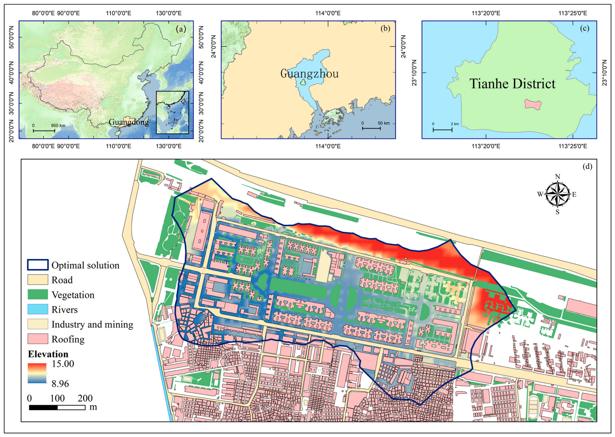
The study area is in Guangzhou City, Guangdong Province, China, and belongs to a south subtropical monsoon climate with abundant annual precipitation and frequent sudden rainstorms in summer. In 2023, influenced by the remnant circulation of Typhoon Haikui combined with southwest monsoon winds, persistent heavy rainfall swept across Guangdong Province from east to west, causing severe urban flooding in Shenzhen, Guangzhou, and other cities; the maximum cumulative rainfall in Shenzhen reached 617.3 mm, breaking multiple historical records. The study object is an old residential community in the Tangde sub-district of Tianhe District, with a total area of approximately 0.54 km². The terrain in the area is flat, with ground elevations ranging from 8.90 to 15.00 m. The stormwater main pipelines run east to west through the community, with branch pipes arranged at building-bay intervals. Stormwater runoff from the community flows into wells, is channeled through branch pipelines into the main pipelines, and is ultimately discharged through three outlets located in the southwest corner of the community. Due to the aging drainage network and inadequate sponge-city measures here, drainage conditions are extremely poor; surface waterlogging forms easily after heavy rainfall, presenting substantial flooding hazards.

Land use in the study area is shown in the figure below, and mainly consists of residential areas, industrial/mining areas, roads, and vegetation. The Digital Elevation Model (DEM) data resolution is 5 m. The drainage network data are the latest official data provided by the Guangzhou Water Authority. Regarding land use, this study revised the 2020 land use data based on satellite image comparison and field surveys. On 21 August 2024, heavy rainfall caused urban flooding in the study area (hereafter ‘20240821 rainstorm’). The 20240821 rainstorm was of long duration and high precipitation, reaching 156 mm. According to the field investigation, this event caused extensive surface waterlogging on Tangde South Road and in adjacent commercial and residential areas to the south, with typical depths of 0.2–0.3 m and partial depths exceeding 0.3 m along Tangde South Road, causing enormous economic losses to local businesses and residents. Figure 2 is the study area.

3.2. Modeling Setup

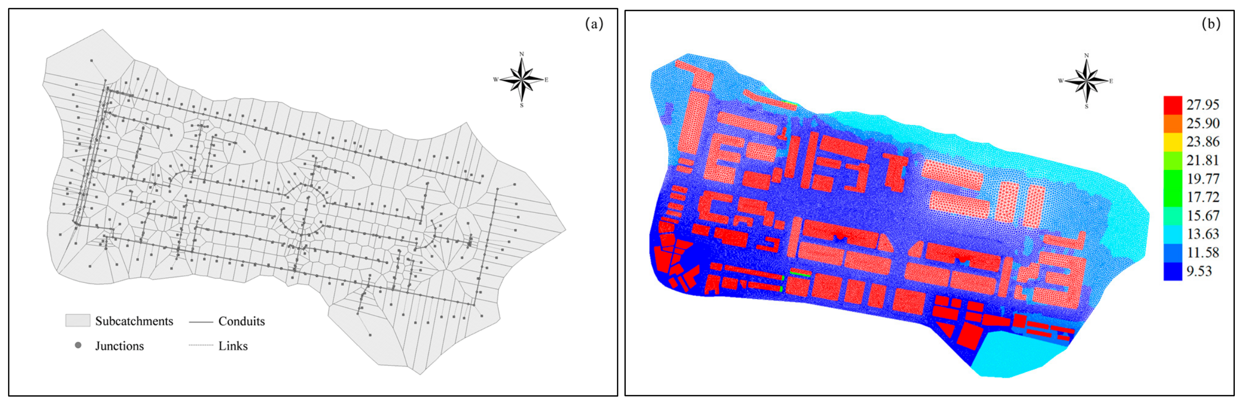
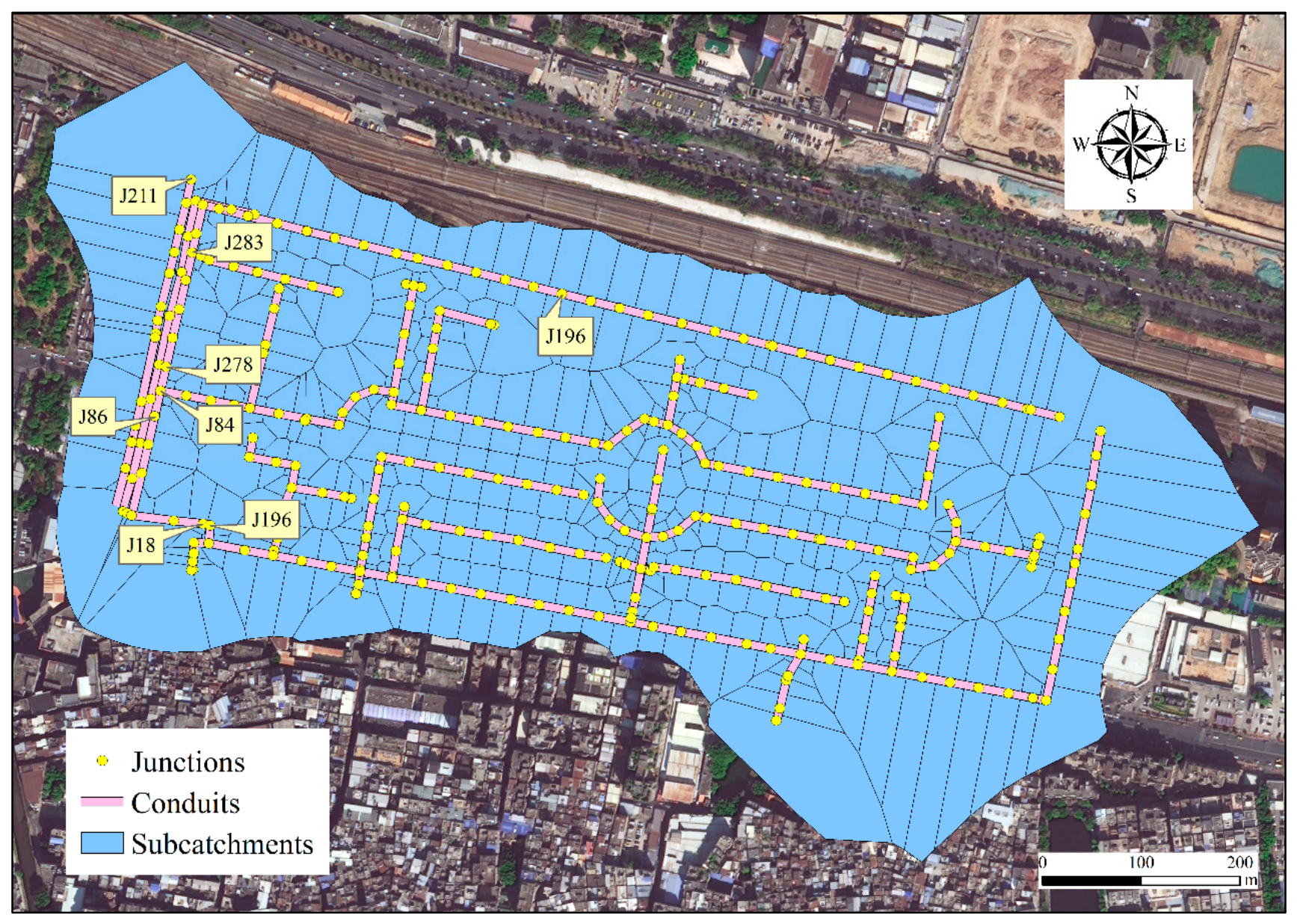
The HORTON infiltration model (an empirical method tailored for infiltration-excess runoff) and the dynamic wave equation were used in the SWMM simulation process. Based on the terrain, land-use planning, building distribution, pipe-network layout, and current drainage zoning, the study area is divided into 292 sub-catchments. To pre-process the basic pipe network data, we only removed 3 completely clogged and abandoned conduits. Following field investigations, it was confirmed that these specific pipes were indeed out of service and lacked any flow exchange with the main drainage network. The final pipe network model consists of 293 stormwater pipes, 295 stormwater manholes, and 3 outfalls. The generalized drainage network model is shown in Figure 3.

For LID facilities, green roofs, permeable pavements, and grass swales are applied. Building rooftops, roads and plazas, and public green spaces are treated as the potential deployment areas for these three LID types, respectively. This approach aims to reduce building roof runoff at the source through green roofs, promote rapid in-situ infiltration and groundwater recharge through permeable pavements, and effectively collect, convey, and pre-treat surface runoff through grass swales, thereby achieving stormwater retention and flood mitigation.

TELEMAC-2D is used to simulate surface overland flow in the study area. An unstructured mesh is constructed within the study area, consisting of 78,419 nodes and 155,570 elements; the base resolution is 5.0 m, locally refined to 1.0 m near roads and flood-prone points. The model was configured with a free outflow boundary, and the initial surface was set to be free of standing water. To avoid double-counting the infiltration losses already calculated in SWMM, and considering that manhole overflows predominantly spread over impervious road networks, no additional infiltration module was applied in the TELEMAC-2D simulation. Rainfall duration is 2 h with a simulation period of 10 h, using a variable time step.

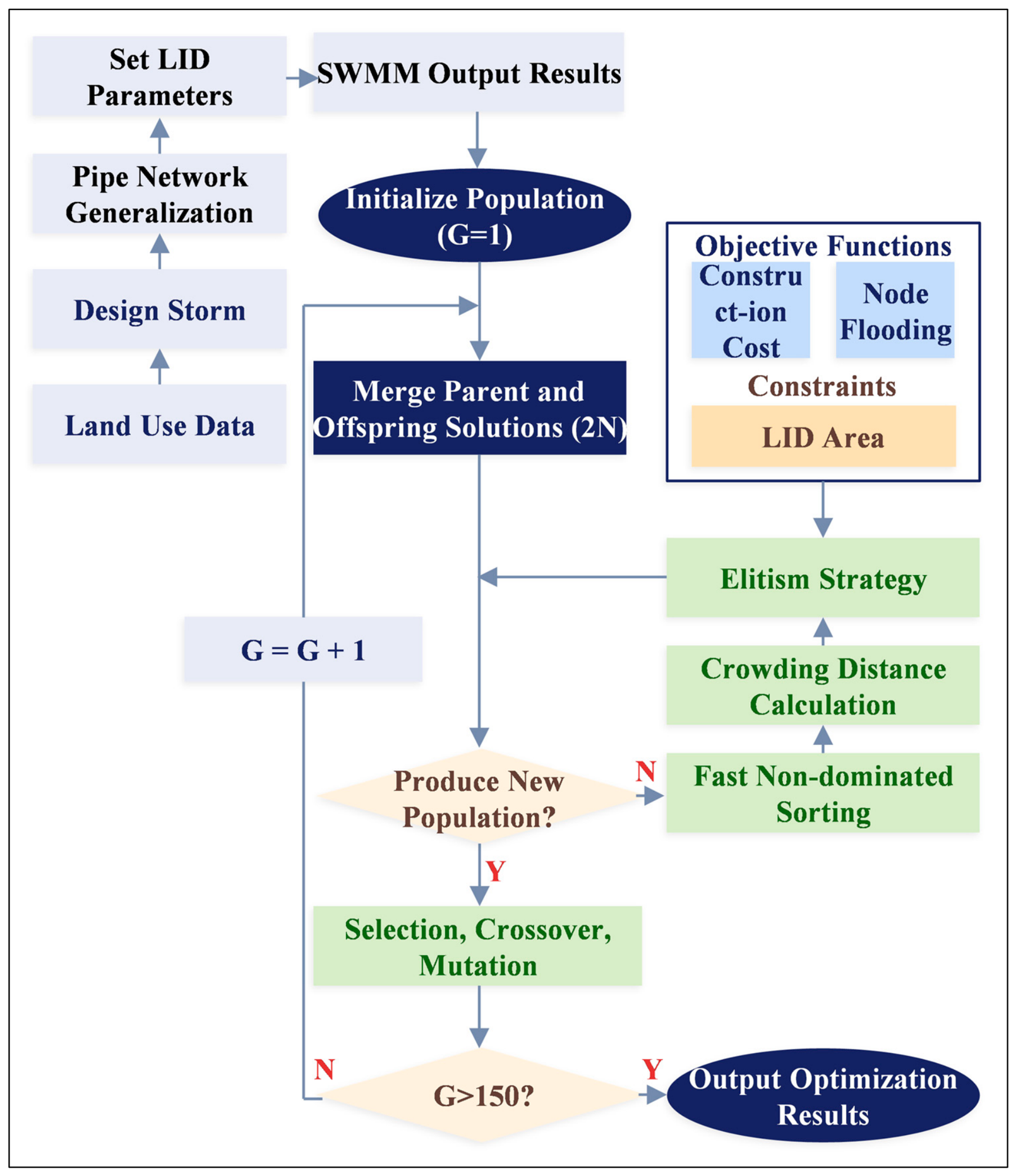
NSGA-II is selected to update schemes and determine optimal LID layout solutions iteratively. The decision variable for the optimization algorithm is the LID deployment area within each sub-catchment, representing the suitable location, type, and size of LID deployment; the actual available land area in each sub-catchment constitutes the constraint. Life-cycle cost (LCC) minimization and total manhole overflow volume minimization are used as objective functions to evaluate each scheme during iteration. SWMM calculates the manhole overflow volume. The LCC is computed as follows.

$$C_{LCC}=C_C+C_{O\&M}$$

(6)

$$C_C={\displaystyle \sum _{i=1}^3}(C_i\times {\mathrm{A}}_i)$$

(7)

$$C_{O\&M}={\displaystyle \sum _{i=1}^3}{\displaystyle \sum _{t=1}^{30}}{\displaystyle \frac{C_i\times {\mathrm{A}}_i\times {\mathrm{P}}_i\times {(1+r)}^t}{{(1+w)}^t}}$$

(8)

where $C_{LCC}$, $C_C$, $C_{O\&M}$ are life-cycle cost, construction cost, and operation-and-maintenance cost (CNY), $C_i$ and ${\mathrm{A}}_i$ are unit area cost (CNY/m²) and total area (m²) of a given LID type; ${\mathrm{P}}_i$ is the coefficient for computing O&M costs, representing the ratio of unit O&M cost to unit total cost; $r$ and $w$ are the inflation rate and depreciation rate, set to 3% and 5%.

Balancing solution precision and computational efficiency, the initial NSGA-II parameters are set as follows: population size 200, number of iterations 150, crossover probability 0.5, mutation probability 0.9.

3.3. Model Calibration and Parameter Assessment

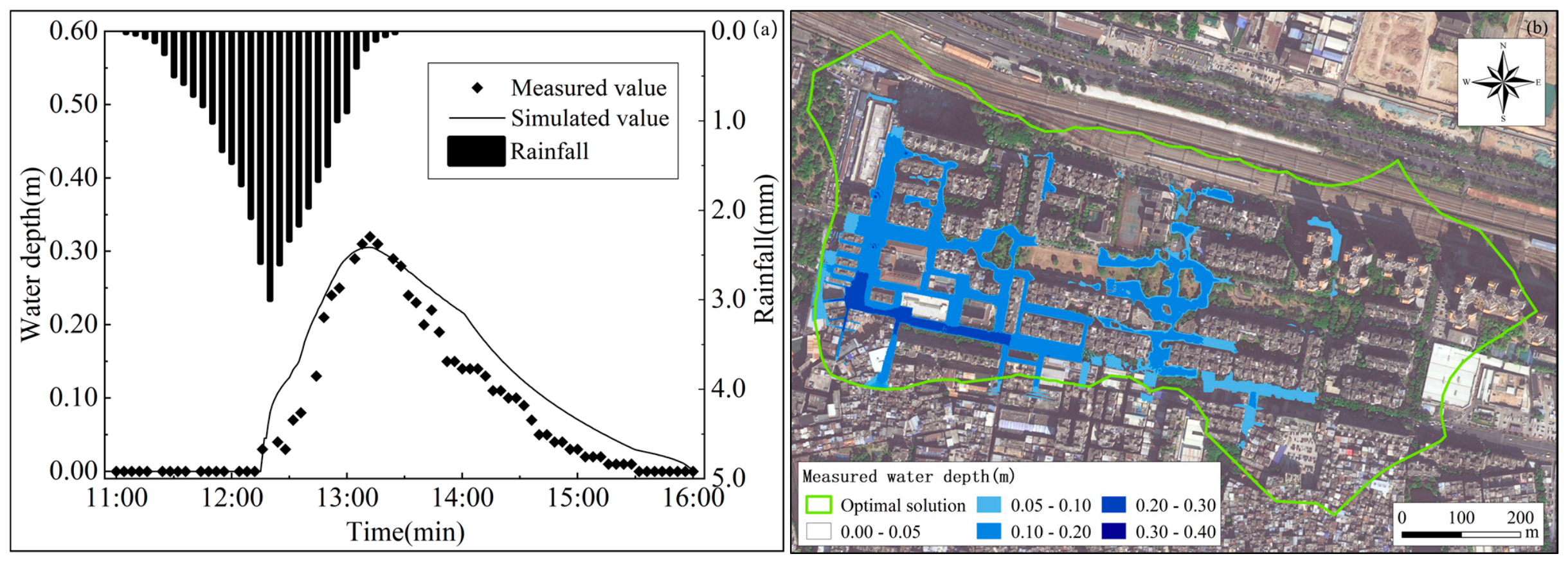
To improve the simulation accuracy and physical reasonableness of the coupled hydrodynamic model, the sub-catchment runoff parameters of SWMM are calibrated. Referring to the official user manual and studies by Niazi, M. [10] and Ren, M. [31], global optimization is performed on key sensitive parameters, including infiltration, depression storage, and Manning’s coefficient for sub-catchments. In addition, key hydrodynamic parameters (e.g., roughness) of TELEMAC-2D are calibrated using observed data, and the coupled model is validated against surface inundation field observations, as shown in Figure 4. The SWMM model parameter calibration results are shown in

Table 1. SWMM Parameters.

Parameter	Meaning of Parameters	Value
N-Imperv	Manning’s coefficient for impervious areas	0.013
N-Perv	Manning’s coefficient for pervious areas	0.41
Dstore-Imperv	Depression storage depth in impervious zones (mm)	1.27
Dstore-Perv	Depression storage depth in pervious zones (mm)	2.54
MaxRate	Maximum infiltration rate (mm/h)	72
MinRate	Minimum infiltration rate (mm/h)	3
Decay Constant	Decay constant	20
Subarea Routing	Subarea routing method	OUTLET

.

The parameter calibration and selection process involved setting initial value ranges based on the official user manual and prior literature, followed by a global optimization procedure. The final values were selected when the coupled model’s outputs achieved the optimal fit with the surface inundation field observations.

The 20240821 rainfall data observed at monitoring stations in Tianhe District are used to validate the reasonableness of the coupled model. The R² and NSE statistical metrics were calculated based on a direct comparison between the simulated time series of water depths and the corresponding in situ measured water depths collected at the Tianhe District monitoring stations during the 20240821 rainfall event. The R² and NSE coefficients are 0.98 and 0.98, respectively. Because the same rainfall event was utilized for both parameter selection and fitting evaluation, and an independent split-sample validation was not performed due to data availability constraints, the model’s absolute quantitative accuracy retains certain limitations. It should be noted that due to the unidirectional form of the coupled model, it is unable to simulate the process of surface water falling back to the pipe network after the decline of well water level in the late stage of the rainstorm event, so the risk assessment based on the simulation results may be high. Consequently, the framework serves primarily as an evaluative tool to capture reasonable runoff trends and approximate intervals, rather than yielding precise numerical predictions for further scenario analysis.

3.4. Rainfall Events Design

The study area is in Tianhe District, Guangzhou, classified as the central urban area. According to «Technical Report on the Compilation of Rainstorm Intensity Formula and Design Rainstorm Patterns for Guangzhou (Abridged Edition)» [32], the rainstorm formula and pattern for the central urban area are:

$$q={\displaystyle \frac{7216.895\times (1+0.555lgP)}{{(\mathrm{t}+29.342)}^{0.841}}}$$

(9)

where $q$ is design rainfall intensity (mm/min), $P$ is return period (years), $\mathrm{t}$ is rainfall duration (min).

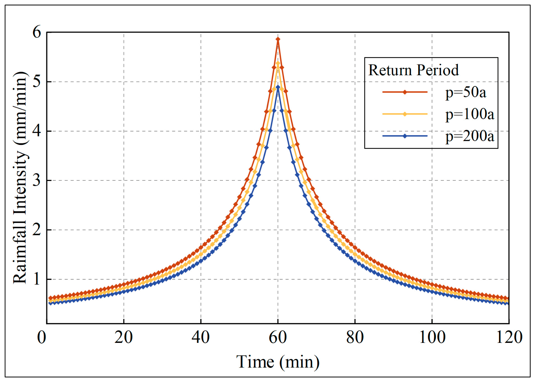
The Chicago Hyetograph Method is used to synthesize rainfall conditions for design return periods of 50, 100, and 200 years. Following Chen, J [33], the peak coefficient is set to 0.5. Rainfall duration and time interval are 2 h and 1 min. The cumulative rainfall amounts for the three storm intensities are 150 mm, 163 mm, and 176 mm, respectively. The storm hyetographs for different return periods are shown in Figure 5.

4. Results and Discussion

4.1. Pareto Front

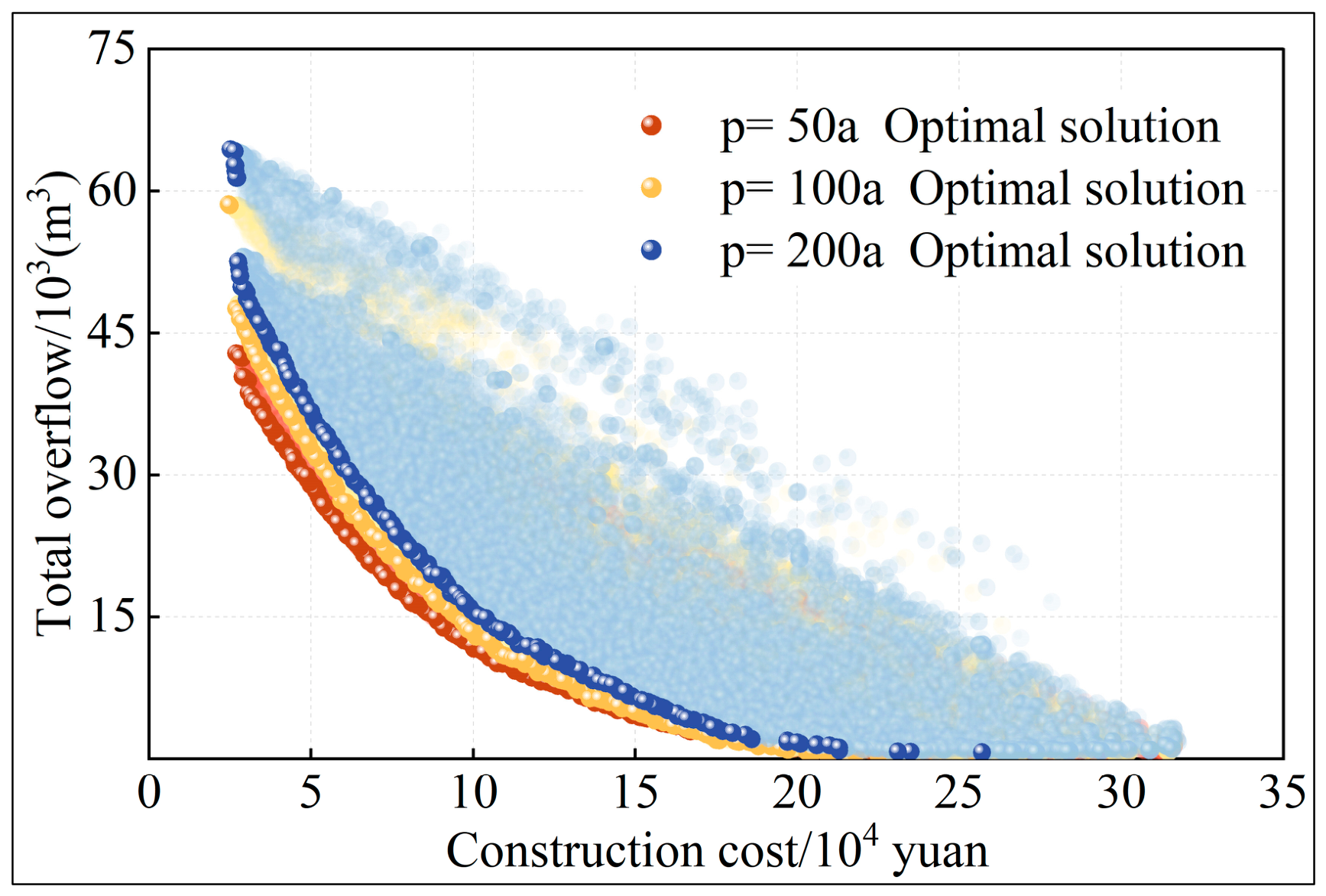
Combining SWMM simulation results with NSGA-II optimization, the final optimized LID layout scheme results are shown in Figure 6. The horizontal and vertical axes represent life-cycle cost (LCC) and total overflow volume (OV), respectively. In this figure, the three point sequences in the lower-left portion represent the optimized scheme under three storm conditions (50-yr, 100-yr, and 200-yr)—the Pareto Front. They characterize the effort to balance the two optimization objectives of “minimum total cost” and “minimum overflow volume”; no single scheme can outperform all others on both objectives simultaneously. The other semi-transparent point sets represent dominated solutions whose results are inferior on both objectives to those on the Pareto Front, and which are ultimately discarded after iteration is complete.

The Pareto Front sequences exhibit diminishing marginal returns; for a constant construction cost of 10 × 10⁴ CNY, the total overflow volume is roughly 15 × 10³ m³ for the 50-year storm, whereas it surges to approximately 20 × 10³ m³ when the return period increases to 200 years, marking an increment of 33%. As total cost increases, the reduction in overflow volume progressively decreases, consistent with the conclusions of Ur Rehman, A. et al. [34]. As storm intensity increases, the Pareto Front shifts upward in the figure. This indicates that with increasing return period, the overflow volume among schemes of equal cost increases; similarly, the total cost of options with the same overflow volume will also rise.

4.2. LID Layout Optimization

A Pareto Front sequence represents the result of the optimization algorithm balancing the two objectives of “lower construction cost’ and ‘better runoff control performance.” Although no scheme is superior to another, schemes at different positions on the curve represent different design strategies (Figure 6). Schemes closer to the upper-left have lower life-cycle costs but greater overflow volumes, representing a preference for “sacrificing runoff control performance to reduce construction and O&M cost.” Schemes at the other end of the curve achieve substantial overflow control effects (even exceeding 95%) at several times the cost, representing a preference for “minimizing overflow regardless of expense.” To further analyze how scheme parameters (LID deployment area and coverage ratio) vary under different strategy preferences, nine schemes representing three strategy preferences are selected from the Pareto Front sequences for three storm return periods. The three strategy preferences are minimum cost, minimum overflow, and balanced compromise, representing the single objectives of “minimize life-cycle cost,” “minimize total overflow volume,” and “pursue the best balance of low cost and high benefit.” These specific points were selected not as absolute statistical representations, but as boundary scenarios and a median trade-off reference for decision-makers. In Figure 6, the schemes at the left and right ends of each curve are treated as the minimum-cost and minimum-overflow schemes, respectively; the inflection point on the curve represents the balanced compromise scheme. The inflection point is identified using the maximum perpendicular distance method: the line connecting the two endpoints of the Pareto curve is used as the baseline; the perpendicular distance from each point on the curve to this baseline is calculated; the point with the maximum distance is taken as the inflection point.

The baseline direction vector is:

$$l=p_m-p_1$$

(10)

For any point $p_i$ on the curve, its perpendicular distance $d_i$ to the baseline is:

$$d_i=‖\left(p_i-p_1\right)-{\displaystyle \frac{\left(p_i-p_1\right)l}{{‖l‖}^2}}l‖$$

(11)

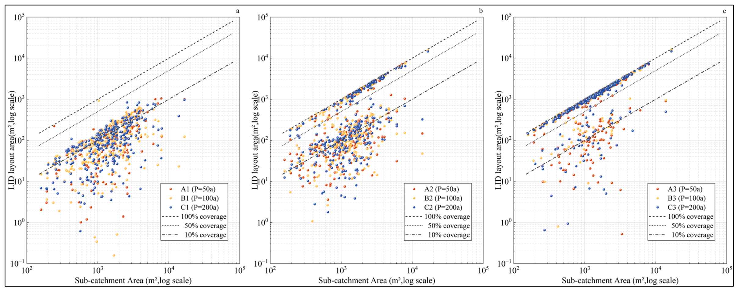
Nine schemes are selected and computed under three storm conditions and three preferences, labeled A0-C3. Here, A, B, and C represent 50-yr, 100-yr, and 200-yr, respectively; 0–3 represent no LID (baseline scheme), minimum cost, balanced compromise, and minimum overflow. The LID areas for each sub-catchment in the results of the nine schemes are shown in Figure 7, where each point represents one sub-catchment.

Under the minimum-cost design strategy, sub-catchment LID areas are relatively similar across the three return periods, with more than 90% of sub-catchments having coverage generally below 10%. Under the balanced compromise scheme (Figure 7b), LID coverage increases overall, concentrated around 10%, with some sub-catchments reaching 100%. In the minimum-overflow results (Figure 7c), the scatter further shifts upward, with most sub-catchments approaching 100% LID coverage. Overall, as the design preference shifts from minimum cost to minimum overflow, LID deployment areas in each sub-catchment show an increasing trend. From the perspective of storm conditions, qualitatively observing, as storm intensity increases, sub-catchment LID coverage also increases overall, though the increment is limited.

When the design strategy is primarily cost-driven, it considers scenarios with limited construction resources in practice, so the total LID facilities available for deployment are limited. When the preference shifts to minimum risk (minimum overflow), it considers mobilizing more resources to protect priority areas, reducing constraints on construction cost, and LID deployment areas exhibit a clear increase. With the increase in rainfall return period, both the total rainfall depth and the total area of green infrastructure deployment exhibit an increasing trend. Based on the combined influence of design preference and storm return period, changes in LID area across the nine schemes will further affect node overflow results within the study area, reflecting flood control effectiveness.

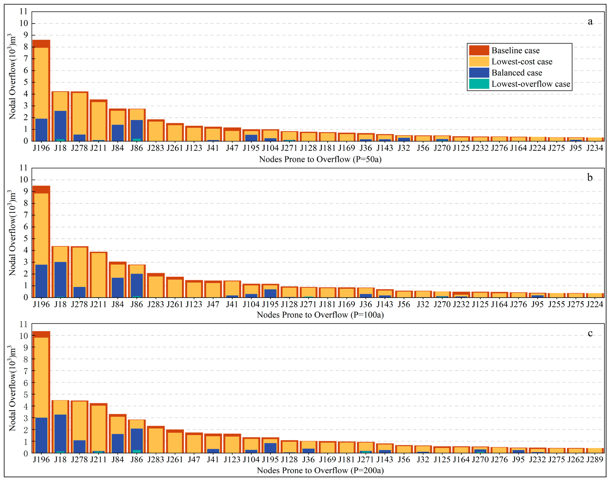
Overflow nodes in the study area are ranked across multiple scenarios in descending order of overflow volume under the baseline condition. The total number of overflow nodes across multiple conditions is approximately 50; the nodes in the latter half have relatively small overflow volumes (not exceeding 0.5 × 10³ m³) with limited impact on area inundation. Therefore, the top 30 overflow nodes are selected for further analysis.

In terms of spatial distribution, nodes with larger overflow volumes (e.g., J196, J18, J278, J211, J84, J86) are concentrated in the mid-to-downstream sections of the pipe network. Although node overflow volumes generally increase as the return period increases from 50 to 200 years, nodes with larger overflow volumes remain consistently ranked near the top across multiple scenarios, while some nodes with smaller volumes change rank. Comparing the results of the three preference schemes, the minimum-cost scheme offers limited overflow reduction, with little change in node overflow volumes; under cost-control as the primary objective, the limited runoff control capacity of LID cannot effectively reduce overflow. In contrast, the balanced scheme shows very clear runoff control effects, with more than 80% overflow reduction at most nodes. After implementing the minimum-overflow scheme, node overflow essentially disappears, though a small number of nodes still overflow; this number increases slightly with storm intensity. There is an upper limit to the runoff control capacity of LID; relying solely on LID remains insufficient to cope with heavy rainfall events, and future considerations could include pipe network upgrades. Figure 8 is node overflow volume.

4.3. Surface Inundation Results

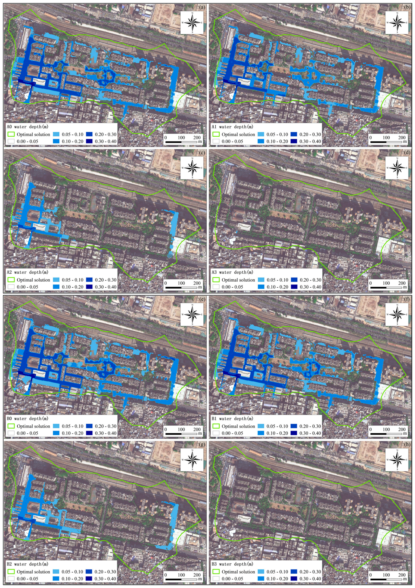
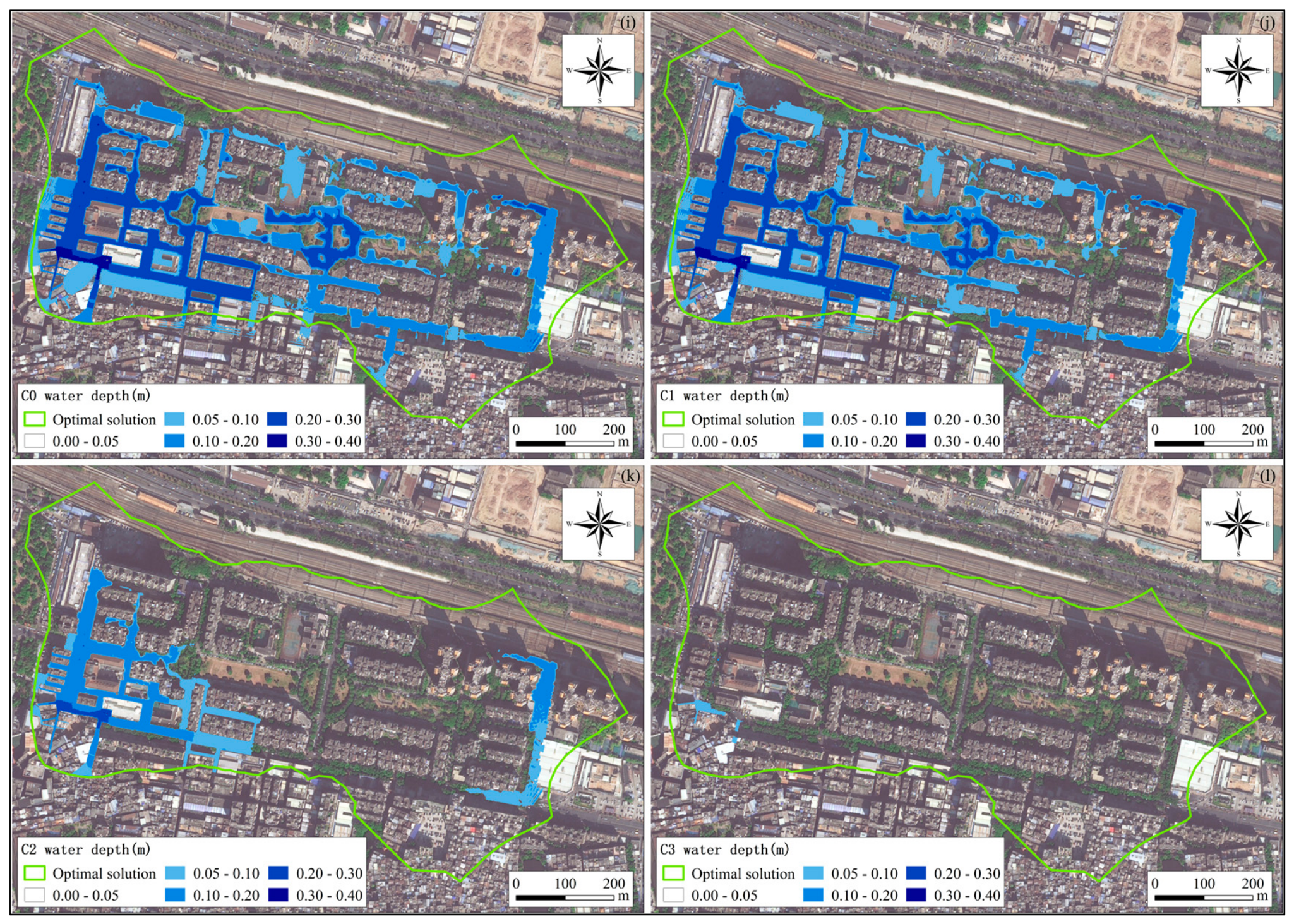
The node overflow results (12 conditions in total) from three storm return periods, three strategy schemes, and the baseline scenario are used as boundary conditions for TELEMAC-2D to simulate surface inundation caused by pipe-network overflow. Considering that inundation in the study area is mainly concentrated in downstream sections of the pipe network, flood-prone points are used as representatives; the moment of maximum water depth for each condition is selected, and the inundation situation under each condition is shown in Figure 9.

Under the baseline condition (no LID) for the 50-year return period, inundation in the study area is mainly distributed in strip patterns along streets, covering the main arterial roads and the southwestern section of the community. The community garden in the central area, due to lower terrain, forms localized inundation with an average depth of approximately 0.2 m, but the green space has a strong water-storage capacity, and ponding recedes rapidly without persistent inundation. A flood-prone point exists at the intersection of the western and southern main arterials—identified from multi-year statistical data—where the terrain is low-lying and receives surface runoff from two directions; the peak inundation depth reaches 0.35 m. As storm intensity increases, the inundation extent under the baseline scheme spreads along streets, and new ponding points appear: at the road junction near the eastern main arterial, and along the southern main arterial in contiguous ponding. Additionally, water depths at many locations also increase. Statistical analysis shows that inundation areas under the 100-year and 200-year scenarios increase by approximately 30% and 40%, respectively, with maximum inundation depths reaching 0.35 m and 0.4 m. Compared to the baseline, the minimum-cost scheme reduces the inundation extent slightly, with the maximum ponding depth in the central garden decreasing from 0.2 m to 0.15 m, but with little change in water depth at the flood-prone point; overall improvement is limited. The balanced scheme reduces inundation extent, with only minor ponding (less than 0.1 m) in the southwestern corner and on the eastern arterial. After implementing the minimum-overflow scheme, only sporadic point-like ponding remains in the study area; the surface ponding coverage is below 5%.

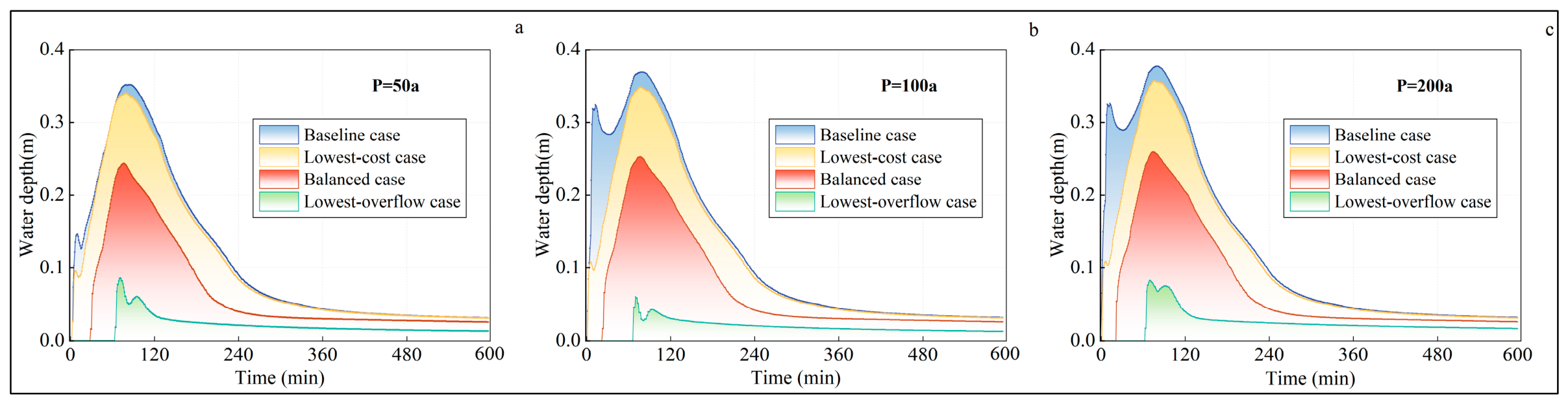
Severe inundation within the study area is concentrated in the southwestern corner, where the flood-prone point is located. Therefore, the flood-prone point is used as a representative for further analysis of temporal variations in water depth within the study area. The water depth results at the flood-prone point under 12 conditions are shown in Figure 10.

As shown in Figure 11, for a 50-year return period storm, the minimum-cost scheme water depth rises rapidly from 30 min, reaches a peak of 0.32 m at 80 min, then gradually decreases to 0.025 m. In comparison, the balanced compromise scheme peaks 10 min earlier; influenced by the optimization preference, the peak depth decreases to 0.24 m, and the minimum drops to 0.020 m. For the minimum-overflow scheme, the flood-prone point accumulates less than 0.1 m of water. As storm intensity increases, the three schemes maintain similar temporal variation patterns; quantitative differences are shown in

Table 2. Statistics of Water Depth at Flood-Prone Locations.

Scheme	P = 50a Peak (m)	P = 50a Time (min)	P = 50a Min (m)	P = 100a Peak (m)	P = 100a Time (min)	P = 100a Min (m)	P = 200a Peak (m)	P = 200a Time (min)	P = 200a Min (m)
Lowest-cost case	0.32	80	0.025	0.33	85	0.03	0.34	90	0.035
Balanced case	0.24	70	0.02	0.27	75	0.025	0.29	75	0.030
Lowest-overflow case	0.05	60	0	0.08	65	0	0.1	70	0.005

.

Specifically, using the 50-year return period as an example, compared to the baseline peak inundation depth of 0.35 m, the minimum-cost scheme only reduces it by 8.6% (to 0.32 m). In contrast, the balanced scheme achieves a reduction of 31.4% (to 0.24 m), while the minimum-overflow scheme demonstrates overwhelming source control capacity, slashing the peak depth by 85.7% (to 0.05 m). Similarly, under the 200-year extreme storm condition, the balanced and minimum-overflow schemes still maintain robust peak depth reduction rates of 27.5% (from 0.40 m to 0.29 m) and 75.0% (to 0.10 m), respectively.

Under the 100-year and 200-year storm conditions, temporal water depth variations at the flood-prone point follow a pattern similar to that of the 50-year event, all showing an initial rise followed by a gradual decline. Intense rainfall causes rapid overflow at pipe-network nodes in a short time, causing surface water depths to increase rapidly; as ponding infiltrates, flows downstream and into lower areas, depth gradually decreases to a stable value. As storm intensity increases, total rainfall in a given time increases, peak values of the water depth curve increase, the rising limb becomes steeper, and the recession time after the peak extends.

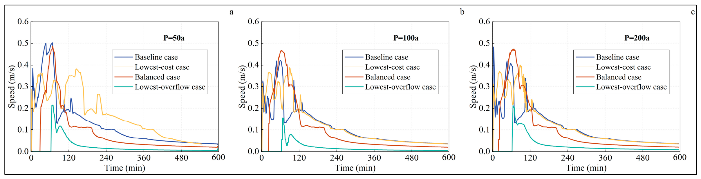
As shown in Figure 12, under the baseline case for the 50-year return period, the flow velocity at the flood-prone point reaches a peak value of approximately 0.5 m/s at around 60 s, and then gradually decreases. Except for the lowest-overflow case, where the peak velocity is reduced to 0.21 m/s, the flow velocities under the other strategy preference schemes show only marginal reductions. The velocity variation patterns under the 100-year and 200-year scenarios are similar to those observed under the 50-year scenario.

4.4. Research Limitations

The coupled modeling framework presented in this study exhibits several inherent limitations. Firstly, the one-way coupling from SWMM to TELEMAC-2D does not allow surface ponding to re-enter the drainage network, tending to overestimate inundation extent, duration, and the required mitigation infrastructure funds. Future work could consider constructing a bidirectional coupling model to address this gap. Secondly, as noted in Section 3.3, model parameters were calibrated using a single observed event without an independent validation dataset, which limits the generalized predictive accuracy of the model. Thirdly, selecting schemes based on the endpoints and inflection point of the Pareto Front offers limited statistical representativeness. Because costs and overflow volumes across different storm conditions are not strictly equated, comparative trends and numerical values may exhibit minor distortions. Lastly, flow velocity at flood-prone points is highly sensitive to local terrain and routing, resulting in fluctuations that this study does not explore in depth. Given these constraints, all calculated metrics and conclusions drawn—including multi-scenario comparisons—should be viewed as qualitative, case-specific rough interval estimates, providing directional guidance rather than exact quantitative universal rules.

5. Conclusions

Based on the SWMM model with life-cycle cost and total overflow volume as optimization objectives, this study employs NSGA-II to optimize LID layout schemes in the study area under three storm return periods, and uses TELEMAC-2D to simulate the surface inundation process under the optimized LID layouts. The main conclusions are as follows:

(1)

The results demonstrate that the SWMM + NSGA-II approach can efficiently explore optimal LID layouts, providing a reference framework for urban flood control scheme design. Meanwhile, the loosely coupled SWMM + TELEMAC-2D model can capture reasonable trends of urban pipe-network runoff generation and routing as well as surface overland flow processes, offering an exploratory approach for estimating qualitative trends and potential intervals of urban inundation. The model holds potential for application in comparable settings with similar physical conditions, specifically urban pipe network data, high-resolution DEM, and hourly precipitation records.

(2)

Based on the results of the numerical example in this study, LID deployment differs under different preference orientations. In the minimum-cost scheme, sub-catchment LID coverage is generally below 10%; in the balanced compromise scheme, coverage is concentrated near 10% with some sub-catchments reaching 100%; in the minimum-overflow scheme, LID coverage approaches 100% in nearly all sub-catchments. Qualitatively speaking, though exact quantitative comparisons are limited by the non-equated costs across scenarios under the same strategy preference, LID deployment area increases with the return period but only moderately.

(3)

Based on the results of the numerical example in this study, runoff control effectiveness varies among schemes with different design preferences. Compared to the baseline, the minimum-cost scheme offers limited runoff control; under the balanced compromise scheme, more than 80% of overflow at most nodes is reduced and the inundation extent decreases; under the minimum-overflow scheme, node overflow and surface ponding are reduced, with peak water depths at the flood-prone point dropping to 0.05 m, 0.08 m, and 0.10 m under 50-yr, 100-yr, and 200-yr storm conditions, respectively.