Toward Sustainable Electromobility: Planning Electric Vehicle Charging Infrastructure with a Hierarchical Bayesian Model, Agent-Based Simulation and Multi-Criteria Decision Making

Abstract

Electromobility is central to urban decarbonisation, but its charging infrastructure must be sized under substantial uncertainty about user behaviour that varies across stations, time of day and user type. This study couples a hierarchical Bayesian model with an agent-based, discrete-event simulation of a charging network. It is fitted by Markov chain Monte Carlo to the public ACN-Data dataset (13,694 sessions across 52 stations; 16,468 user requests), with partial pooling across stations. Posterior parameters drive a 24 h simulation of 500 vehicles across nine configurations and 30 to 180 slots. Service success rises from 19% to 81% and mean waiting falls from 110 to 62 min; long workplace dwell times limit turnover, so capacity rather than energy binds. TOPSIS with a paired bootstrap selects 160 slots under balanced weighting, but that optimum holds for only a tenth of the weight simplex, and the recommendation spans 140–180 slots. Spreading the arrival peak at fixed hardware raises service from 67% to 83%, matching a 29% expansion. Spatially explicit assignment costs three percentage points when stations are evenly sited, and six when clustered. The framework makes the cost of over-provisioning explicit and preference-conditional rather than naming a single optimum, giving a reproducible basis for sustainable capacity planning.

1. Introduction

Public interest in electric vehicles (EVs) has grown rapidly in recent years, driven by the need to reduce greenhouse-gas emissions and improve urban air quality, and reinforced by falling battery costs that make electricity an increasingly competitive transport fuel. Yet charging infrastructure has struggled to keep pace with vehicle adoption, so that the number, type, location and availability of charging stations frequently fail to match local demand—either falling short of it or, conversely, being over-provisioned at considerable cost. The central motivation of this work is to build tools that predict and model these situations before they materialise, so that both under- and over-investment can be avoided.

The scale of this planning problem is no longer marginal. Global sales of electric cars neared 14 million in 2023, reaching 18% of all cars sold, while the public charging stock grew by more than 40% over the same year and the number of fast chargers by 55% [1]. Deployment at this rate means that sizing decisions are being taken continuously and in large numbers, so that a systematic bias in how they are made—towards idle hardware on one side or unserved drivers on the other—accumulates quickly into stranded capital or suppressed adoption. The dataset analysed in this work illustrates the operational face of the same problem. Across 13,694 workplace charging sessions the median connection lasts more than eight hours, so a single slot can serve only a handful of vehicles per day. What limits a network is therefore how many vehicles it can accommodate at once during the demand peak, not the energy it could deliver over a full day. It is this concurrency constraint, and the behavioural uncertainty that surrounds it, that a planning tool has to represent.

Electrifying road transport is a cornerstone of sustainable urban development and contributes directly to the United Nations Sustainable Development Goals on affordable and clean energy (SDG 7), sustainable cities and communities (SDG 11) and climate action (SDG 13). Realising these benefits, however, depends not merely on deploying chargers but on deploying them efficiently. Over-built infrastructure wastes scarce materials, capital and embodied carbon and leaves chargers idle, whereas under-built infrastructure strands drivers, lengthens queues and slows the very adoption that decarbonisation requires. Sustainable electromobility therefore hinges on right-sizing charging networks under uncertainty—matching capacity to real, variable demand so that service is delivered with the least resource and financial cost. This resource-efficiency perspective, rather than charging technology alone, frames the present study and places it squarely within the sustainability agenda: the tool developed here is intended to help planners avoid both the environmental cost of over-provisioning and the mobility cost of under-provisioning.

Charging stations differ substantially in power, charging method and purpose. Alternating-current (AC) stations, typically rated between roughly 3.7 kW and 22 kW, are used mainly for slower charging over longer dwell times, whereas direct-current (DC) fast chargers, ranging from 50 kW to more than 300 kW, drastically shorten charging time but impose a much heavier and more concentrated load on the distribution network. Alongside these technical differences, stations differ in how they are used, in their grid requirements and in their installation and operating costs [2]. From the grid perspective, the key concern is the power balance at a distribution node: a sharp rise in the number of simultaneously charging vehicles can cause local overload, voltage drops and transformer overloading, and this risk is aggravated by the temporal concentration of charging, since many users begin charging in the evening after returning home, producing pronounced peaks in demand [3].

The demand for charging therefore varies strongly with time, location, traffic conditions, user type and the technical characteristics of the vehicles themselves, and user behaviour cannot be treated as fully predictable or constant. This high variability is why classical deterministic models—which assume fixed values or average system behaviour—often fail to describe real charging operation accurately: they cannot adequately represent uncertainty, differences between locations, or temporal changes in demand [4]. For this reason, probabilistic and statistical models that work directly with real data and capture the complexity of user behaviour have gained increasing importance. Simulation and modelling make it possible to predict system behaviour before infrastructure is built and to test many scenarios—varying the number and type of stations, the number and behaviour of vehicles, battery capacities and other conditions—thereby avoiding both incorrect capacity calculations and unnecessary planning costs.

Among the probabilistic methods that have recently gained traction in demand analysis and forecasting, the hierarchical Bayesian model (HBM) is one of the most developed. It allows several levels of data to be integrated and different behaviour-shaping factors to be accounted for, and its hierarchical structure provides considerable flexibility when working with complex, large and multi-level datasets while still enabling unobserved quantities to be estimated from available observations. Hierarchical probabilistic approaches have been applied successfully to characterising charging flexibility [5], to scalable probabilistic estimation of charging from observed driver behaviour [6], and to coherent multi-scale forecasting of charging demand [7,8]. The present work adopts this paradigm and couples it with a simulation environment so that the inferred behaviour can be exercised under arbitrary infrastructure configurations.

The aim of this work is to design, build and test a simulation that uses the principles of a hierarchical Bayesian model to analyse the utilisation of EV charging stations. This makes it possible to better understand user behaviour, identify regularities in demand and propose more effective solutions for the development of the charging network. The work is decomposed into six tasks. The first is to survey existing approaches to modelling and simulating charging-station usage, with their advantages and limitations. The second is to obtain a dataset of real charging-station usage covering start time, duration, energy consumed, station location and vehicle attributes. The third is to construct a hierarchical Bayesian model that captures multi-level variability, for example between stations and between time periods. The fourth is to design a simulation environment in which the model outputs can be exercised and interpreted. The fifth is to assess the accuracy, reliability and added value of the proposed model relative to other statistical or deterministic approaches. The sixth is to formulate recommendations for more efficient planning of charging infrastructure. The expected result is a functional modelling tool, based on a hierarchical Bayesian model, that reproduces probable user behaviour as faithfully as possible and provides a basis for infrastructure-development decisions.

The remainder of the paper is organised as follows. Section 2 analyses the main modelling paradigms—agent-based modelling, queueing theory and stochastic simulation—and introduces the theoretical basis of hierarchical Bayesian models. Section 3 describes the materials and methods: the ACN-Data dataset, the hierarchical Bayesian station and vehicle models, the agent-based discrete-event simulator, and the simulation scenarios. Section 4 presents the results of the nine simulation scenarios. Section 5 discusses the findings, their implications for capacity planning, and the advantages and limitations of the approach. Section 6 concludes.

2. Related Work and Theoretical Background

Modelling the demand for EV charging stations is a complex task influenced by many factors—user behaviour, trip patterns, vehicle type and model, electricity price and station availability. The literature offers a broad range of approaches that can be classified by several criteria; the three most relevant paradigms are summarised below, followed by the theoretical basis of hierarchical Bayesian modelling adopted in this work.

2.1. Agent-Based Modelling

Agent-based modelling (ABM) is a natural approach to simulating charging stations because it represents the behaviour of individual “agents” (EV drivers) and their interaction with the charging stations within a single system. Each vehicle is modelled as an autonomous agent with its own behavioural rules, derived from real data such as daily trip patterns, charging preferences and willingness to risk battery depletion; agents move through a digital representation of the transport network and decide when and where to charge on the basis of their current state (e.g., state of charge) and their surroundings (e.g., availability of chargers, price, distance to the nearest station) [2]. The strengths of ABM are its flexibility in representing heterogeneous driver behaviour, its ability to study emergent phenomena such as queue formation and localised grid overload, and its usefulness for policy analysis [3]. Its weaknesses are computational cost for large agent populations, the substantial data required for calibration and validation, and the difficulty of interpreting results that emerge from many interacting variables. Agent-based modelling has been used effectively for cost-effective siting of charging infrastructure [3].

2.2. Queueing Theory

Queueing theory provides an analytical basis for modelling systems in which clients (EVs) arrive to obtain a service (battery charging) from service facilities (charging stations). Stations are modelled as service systems characterised by an input process (e.g., a Poisson arrival process), a service-time distribution (charging duration) and a number of service lines (charging points per station); from these, indicators such as the mean queue length, mean waiting time and station utilisation can be evaluated analytically [4]. The strengths of this approach are speed and efficiency—it provides rapid performance estimates without complex simulation—and its usefulness for determining the optimal number of stations for an expected demand. Its weaknesses are the simplifying assumptions it usually relies on (stationary demand, exponential service times) and its limited ability to capture strategic driver behaviour, both of which can introduce inaccuracies.

2.3. Stochastic Simulation Models

Stochastic simulation models explicitly account for randomness and variability in processes such as arrival times and charging durations. Key input parameters (daily mileage, initial state of charge, charging start time) are represented as probability distributions, and the simulation is repeated many times (Monte Carlo method) to obtain a distribution of possible outcomes and to evaluate system variability [6]. The strengths of this approach are its quantitative treatment of uncertainty—it evaluates not only mean values but also risks, such as the probability that the number of vehicles exceeds station throughput—and its more realistic forecasts compared with deterministic models. Its weaknesses are the demand for reliable data to estimate the distribution parameters, and the computational cost of large numbers of simulations. Reviews of open EV-charging data and models emphasise that the reliability of any such approach rests on the quality and openness of the underlying datasets [2].

The three paradigms above all describe how a charging network behaves once its layout is given. A substantial and rapidly growing literature addresses the complementary questions of where stations should be placed and how they should be operated. Location-selection studies combine demand, geographic and cost criteria to site stations, and have recently begun to use generative artificial intelligence to propose and screen candidate configurations that conventional search procedures do not reach [9]. Work on charging-station energy management systems addresses operation rather than placement, dispatching between grid supply, on-site generation and storage using mathematical programming, metaheuristics and reinforcement learning [10]. Both strands are complementary to the present study rather than alternatives to it: they answer where to build and how to run, whereas the question here is how much capacity a network needs before service quality becomes acceptable under uncertain demand. A third body of work approaches the same system from the demand side, showing that time-of-use tariffs measurably reshape when and where drivers charge and that this price response is strongly heterogeneous across user segments [11]. That evidence bears directly on the demand-shifting lever discussed in Section 5.1. The framework developed here treats the arrival-intensity profile as an exogenous input, so a tariff-induced change in arrival timing can be evaluated simply by reshaping that profile; the behavioural price-response model that would generate the reshaping is taken from the cited literature and is not re-estimated in this work, which is a deliberate boundary of scope rather than an omission.

No single approach is universally best; the choice depends on the specific research task, the available data and the required level of detail. Important nuances include scalability (a model calibrated for one city may not transfer to another), sensitivity to dynamic electricity prices, and the degree to which charging demand is coupled to an explicit grid model. The present work therefore combines the paradigms: a hierarchical Bayesian model supplies uncertainty-aware, data-driven behaviour, and an agent-based discrete-event simulator exercises that behaviour to produce emergent, network-level indicators.

2.4. Hierarchical Bayesian Models

Data from charging infrastructure are typically structured—observations are grouped by station, day of week, user type or location—which makes hierarchical Bayesian models (HBMs) a particularly effective tool. Whereas classical (frequentist) statistics treats parameters as fixed but unknown, the Bayesian approach treats them as random variables to which a probability distribution is assigned, expressing uncertainty about their values. The cornerstone is Bayes’ theorem,

$$P(\theta \mid D)={\displaystyle \frac{P(D\mid \theta )P\left(\theta \right)}{P\left(D\right)}}$$

where P(θ|D) is the posterior—the updated probability of the parameters θ after observing data D; P(D|θ) is the likelihood; P(θ) is the prior; and P(D) is the evidence, a normalising constant. In practice P(D) is rarely computed explicitly, since for inference only the shape of the posterior matters, which is proportional to the product of the likelihood and the prior—the basis of the numerical approximation methods common in Bayesian statistics. A further advantage is sequential updating: as new data arrive, the previous posterior becomes the new prior, which is especially suitable for a dynamic system such as EV charging where user behaviour changes over time [5].

Hierarchical Bayesian models extend this by introducing several levels of parameters. Their central idea is that lower-level parameters (e.g., of individual stations) are not independent but are drawn from a higher-level distribution representing shared properties of the whole system. For charging infrastructure the hierarchy may run from individual charging events, through charging stations, to geographical areas and finally to global network characteristics; each level captures a different degree of variability and uncertainty. Formally a simple hierarchical model can be written as

$$y_{ij}~\mathcal{N}({\mu }_{ij},\sigma ),{\theta }_j~\mathcal{N}(\mu ,\tau )$$

where $y_{ij}$ is the i-th observation in group j, ${\theta }_j$ are group-specific parameters (e.g., of a particular station) and μ and τ are global hyperparameters. A key advantage of this structure is partial pooling, a compromise between complete pooling (all observations treated as identical) and no pooling (each group modelled separately). The mechanism is shrinkage: because the group-level parameters are assumed exchangeable and drawn from a common distribution whose own parameters are estimated from the data, each station estimate is pulled from its noisy individual value towards the network mean by an amount that depends on how much data the station provides. Data-rich stations are shrunk little and retain their own character, whereas data-poor stations “borrow strength” from the rest of the network and are modelled more stably and less extremely. This adaptive regularisation is the property that lets the model produce reliable estimates for stations—and, by extension, for hypothetical future stations—that individually carry little information.

The prior P(θ) encodes what is known about the parameters before the data are seen. This work uses weakly informative priors: distributions that are broad enough not to bias the result yet tight enough to keep the sampler within a physically plausible region and to regularise estimates when data are sparse. Where observations are abundant the likelihood dominates and the prior’s influence vanishes; where they are scarce the prior prevents implausible values. A Bayesian model is moreover generative—it specifies a complete joint distribution over parameters and data—so that once the posterior is obtained the model can be both checked and used through the posterior predictive distribution, which propagates parameter uncertainty into predictions by averaging the data-generating distribution over the posterior. In the implementation reported here the simulator is parameterised by the posterior means of the fitted effects, while the session-level residual terms estimated by the models (σ_res for delivered energy, σ_f for fulfilment) are resampled at every simulated session. The simulation is therefore driven by the aleatoric variability the models quantify, rather than by the full epistemic uncertainty of the parameters themselves. Because the posteriors are very tightly identified at these sample sizes (

Table 1. Posterior parameters of the hierarchical Bayesian station model (fitted to 13,694 sessions across 52 stations). The 94% credible interval is the 3rd–97th posterior percentile.

Parameter	Symbol	Posterior Mean	94% Credible Interval
Global base energy	base_kwh	9.17 kWh	[8.94, 9.42]
Duration coefficient (log-kWh per SD of dwell time)	b	0.301	[0.276, 0.325]
EV-pressure (network-load) effect	β_p	−0.0085	[−0.034, +0.015]
Connection-type effect (discharging)	β_c	−0.534	[−0.555, −0.510]
Charging-type effect (fast)	β_f	1.182	[1.157, 1.207]
Duration × charging interaction	β_df	0.302	[0.280, 0.324]
Residual noise (log scale)	σ_res	0.523	[0.516, 0.529]

and

Table 2. Posterior parameters of the vehicle fulfilment model under the normal specification (fitted to 16,468 user requests). The 94% credible interval is the 3rd–97th posterior percentile. Section 3.4.3 refits the same mean function with a Beta likelihood and adopts it; the Beta posterior means are μ₀ = 0.402, μ_k = −0.436, μ_m = 0.242, μ_w = −0.255, γ_c = −0.310, γ_f = 0.522 with precision φ = 4.18, and it is these values that parameterise the simulator.

Parameter	Symbol	Posterior Mean	94% Credible Interval
Base fulfilment (logit)	μ0	0.362	[0.345, 0.380]
Requested-energy effect	μ_k	−0.561	[−0.585, −0.538]
Available-time effect	μ_m	0.289	[0.273, 0.305]
Wh-per-mile effect	μ_w	−0.272	[−0.286, −0.257]
Connection-type effect	γ_c	−0.351	[−0.390, −0.314]
Charging-type effect	γ_f	0.616	[0.578, 0.654]
Fulfilment noise	σ_f	0.207	[0.205, 0.210]

), the two coincide closely in this case; carrying the complete posterior predictive distribution through the simulator is nonetheless the more general procedure, and is identified as an extension in Section 5.3.

Because a hierarchical posterior rarely has a closed form, it is approximated by drawing samples with MCMC. Classical samplers such as Metropolis–Hastings and Gibbs sampling explore the parameter space by a random walk; in the high-dimensional, strongly correlated posteriors typical of hierarchical models they mix slowly and can leave regions unexplored. Gradient-based Hamiltonian Monte Carlo (HMC) instead treats the negative log-posterior as a potential energy and simulates Hamiltonian dynamics, using the gradient to propose distant states that are accepted with high probability; the No-U-Turn Sampler (NUTS) removes HMC’s main tuning burden by automatically choosing the trajectory length, and is the default in modern probabilistic-programming systems [12,13]. Convergence of the resulting chains is verified with standard diagnostics: the potential scale reduction factor $\widehat{\mathrm{R}}$, which compares within- and between-chain variance and must be close to one [14]; the effective sample size, which measures the information carried by autocorrelated draws; and the count of divergent transitions, which flags geometry the sampler cannot traverse.

Hierarchical probabilistic approaches have been applied to characterising charging flexibility [5], coherent multi-scale demand forecasting [7,8] and spatiotemporal load forecasting [15], confirming their suitability as the theoretical basis for the model designed here.

2.5. Multi-Criteria Decision Making for Infrastructure Planning

Sizing a charging network is not a single-objective optimisation. A configuration is judged simultaneously on conflicting criteria—the quality of service (the share of vehicles served, to be maximised, and their waiting time, to be minimised) and the cost (the capital tied up in stations and slots, to be minimised)—and improving one generally worsens another. Multi-criteria decision making (MCDM) provides the formal apparatus for exactly this kind of problem and is widely used in sustainable-energy planning [16].

The foundational concept is Pareto optimality. A configuration is Pareto-optimal (non-dominated) if no other configuration is at least as good on every criterion and strictly better on at least one; the set of non-dominated configurations forms the Pareto front, and any defensible choice must lie on it. Selecting a single point on the front requires expressing preferences among the criteria, for which several aggregation methods exist.

The simplest is the weighted-sum model: each criterion is normalised—benefit criteria increasing, cost criteria inverted—and combined into a scalar score using weights that sum to one. The weights themselves can be elicited with the Analytic Hierarchy Process (AHP), which derives them from pairwise comparisons of the criteria on a ratio scale, extracts them as the principal eigenvector of the comparison matrix, and checks their logical consistency [17]. A more discriminating aggregation is the Technique for Order of Preference by Similarity to Ideal Solution (TOPSIS) [18]. After the decision matrix is vector-normalised and weighted, TOPSIS defines an ideal solution (the best attainable value on every criterion) and an anti-ideal solution (the worst on every criterion); each alternative i then receives a closeness coefficient

$$C_i={\displaystyle \frac{d_i^{-}}{d_i^{+}+d_i^{-}}}$$

where $d_i^{+}$ and $d_i^{-}$ are its Euclidean distances to the ideal and anti-ideal solutions. The coefficient lies in [0, 1], and the alternative with the highest value—closest to the ideal and farthest from the anti-ideal—is preferred. Methods of this family are established tools for the siting and sizing of EV charging infrastructure [16,19]. Because any such ranking depends on the chosen weights, a sensitivity analysis over plausible weightings is essential: a configuration preferred across a broad range of weights is a robust choice. Section 5.4 applies TOPSIS to the nine simulated scenarios to identify the compromise region, and Section Robustness of the Ranking to Simulation and Weight Uncertainty tests how firmly that identification is supported by the underlying simulation.

3. Materials and Methods

The complete system was implemented in Python (ver. 3.14.6) using the PyMC (ver. 6.3.1), NumPy (ver. 2.5.2), Pandas (ver. 3.0) and Matplotlib libraries (ver. 3.11.1). It consists of two parts: a hierarchical Bayesian model that estimates charging and vehicle-behaviour parameters from historical data, and an agent-based discrete-event simulator that uses the inferred parameters to simulate the operation of a charging-station network over a 24 h horizon.

3.1. Dataset

The model was fitted to the public ACN-Data dataset, an open EV-charging dataset collected from adaptive charging networks [20]. Each record describes a charging session and provides the station identifier, delivered energy, connection and disconnect times, an EV-pressure estimate, the connection and charging type, and user inputs such as requested energy and available time. Sessions were loaded from JSON, converted to a data frame and cleaned: session duration was derived from the connection and disconnect timestamps, and records were retained only if the duration lay between 0.1 h and 48 h and the delivered energy between 0 kWh and 80 kWh. These limits are physical plausibility bounds rather than statistical outlier criteria. A connection shorter than six minutes reflects an aborted plug-in rather than a charging event, and one longer than 48 h indicates a vehicle left plugged in across a weekend or a metering fault. The 80 kWh ceiling exceeds the usable battery capacity of the vehicles represented in ACN-Data, so larger values indicate metering errors or concatenated sessions. No record was excluded because of its influence on the fit. In this dataset the rules are in practice almost inert: they remove 5 of 13,699 sessions (0.04%), all of them through the 48 h limit, so none of the reported results is sensitive to the exact thresholds. Categorical variables (station, connection type, charging type) were encoded numerically, and the continuous predictors (duration, EV pressure) were standardised; the response was modelled on the log scale via log(1 + kWh). After cleaning, the station-level energy model was fitted to 13,694 sessions across 52 stations, and the vehicle fulfilment model to 16,468 user sessions.

3.2. Hierarchical Bayesian Station Model

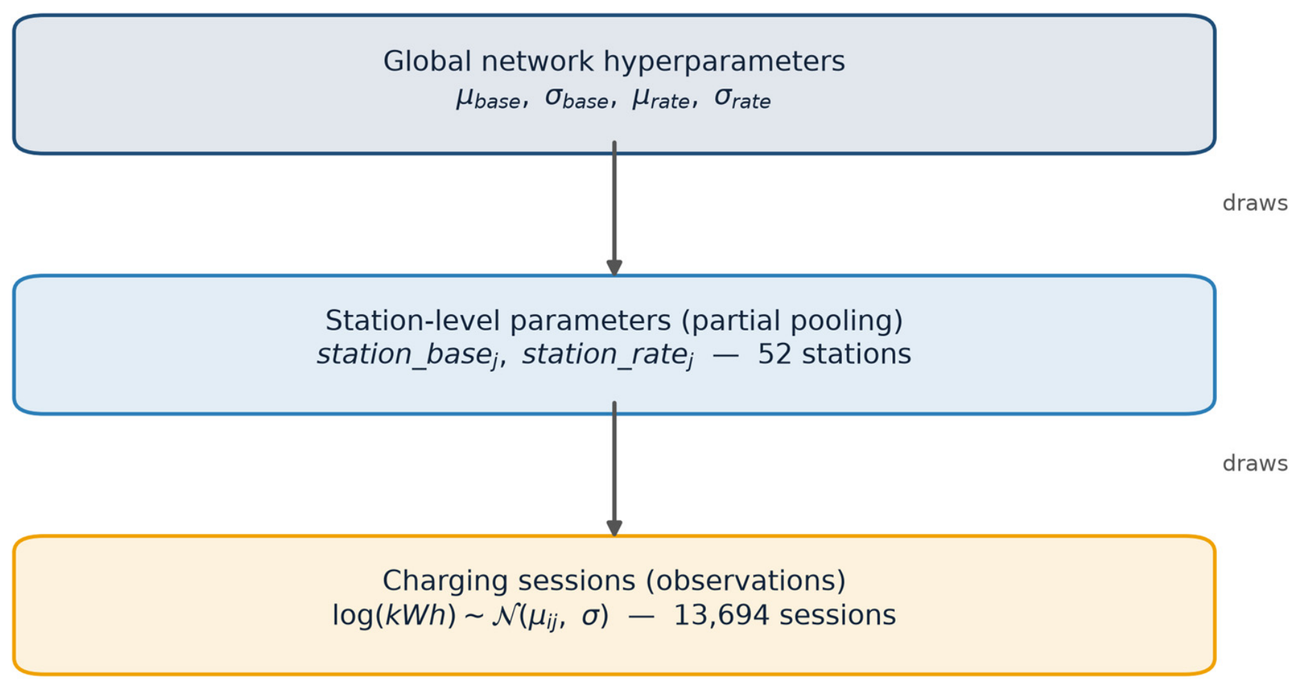
The station model predicts the energy delivered in a session while capturing differences between stations and the global characteristics of the network. Each station j receives its own base parameter a_j and rate parameter b_j, drawn from global hyperpriors: a_j

$$a_j~\mathcal{N}({\mu }_{base},{\sigma }_{base}),b_j~\mathcal{N}({\mu }_{rate},{\sigma }_{rate})$$

with weakly informative hyperpriors μ_base ~ N(2,1), σ_base ~ HalfNormal(0.5), μ_rate ~ N(0.5,0.3) and σ_rate ~ HalfNormal(0.3). Additional session-level effects describe the influence of network load (EV pressure), connection type and charging type, together with a duration–charging interaction:

$${\mu }_{ij}=a_j+b_j{d}_i+{\beta }_p{p}_i+{\beta }_c{c}_i+{\beta }_f{f}_i+{\beta }_{df}{d}_i{f}_i$$

where d_i is the standardised duration, p_i the standardised EV pressure, and c_i and f_i are the connection- and charging-type codes; the effect priors are β_p ~ N(0,0.3), β_c ~ N(0,0.5), β_f ~ N(0.5,0.3) and β_df ~ N(0,0.2). The observed log-energy is modelled as normal,

$$\mathrm{l}\mathrm{o}\mathrm{g}(1+\mathrm{k}\mathrm{W}\mathrm{h}{)}_i~\mathcal{N}({\mu }_{ij},{\sigma }_{res})$$

so that the predicted energy is recovered as kWh = exp(μ_ij) − 1 with multiplicative residual noise. Inference used the No-U-Turn/Hamiltonian Monte Carlo sampler in PyMC (ver. 6.3.1) [21] with 1500 draws, 800 tuning steps, four parallel chains, a target acceptance probability of 0.95 and a fixed random seed. Convergence was verified with the diagnostics introduced in Section 2.4 and is satisfactory throughout: the rank-normalised potential scale reduction factor does not exceed $\widehat{\mathrm{R}}$ = 1.003 for any parameter, the smallest bulk and tail effective sample sizes are 866 and 1270 respectively, and the sampler recorded no divergent transitions in the 6000 post-warm-up draws. The posterior means, which parameterise the simulator, are summarised in Table 1.

3.3. Vehicle Fulfilment Model

A second Bayesian model predicts the fulfilment ratio—the fraction of requested energy that a vehicle actually receives—from user inputs extracted from the session records (requested energy, available time, energy consumption per mile). A linear predictor of the standardised inputs is passed through a logistic (sigmoid) link, and the observed fulfilment ratio is modelled as normal around the resulting mean:

$$F_i~\mathcal{N}(\mathrm{s}\mathrm{i}\mathrm{g}\mathrm{m}\mathrm{o}\mathrm{i}\mathrm{d}({\eta }_i),{\sigma }_f),{\eta }_i={\mu }_0+{\mu }_k{k}_i+{\mu }_m{m}_i+{\mu }_w{w}_i+{\gamma }_c{c}_i+{\gamma }_f{f}_i$$

where F_i is the fulfilment ratio and k_i, m_i and w_i are the standardised requested energy, available minutes and Wh-per-mile, with priors μ_0 ~ N(0.5, 0.3), μ_k ~ N(−0.3, 0.2), μ_m ~ N(0.2, 0.2), μ_w ~ N(−0.1, 0.2), γ_c ~ N(−0.2, 0.2), γ_f ~ N(0.3, 0.2) and σ_f ~ HalfNormal(0.15). The fulfilment ratio is bounded on [0, 1] whereas a normal likelihood centred on a sigmoid mean is not, so the specification can in principle place mass outside the admissible range; the observed ratios were accordingly truncated to [0.05, 0.95] before fitting and simulated draws were constrained to the same interval. With the fitted residual scale (σ_f = 0.207) this is not a negligible correction: 6.1% of the posterior predictive mass of the normal specification lies outside [0, 1] and is removed by the truncation (Section 3.4.3). The reported effects are unchanged by it, but a Beta likelihood respects the support by construction, and the model was accordingly refitted in that form; Section 3.4.3 reports the comparison and adopts it. The posterior means are given in Table 2; the mean observed fulfilment ratio in the data was 0.61, reflecting that vehicles frequently disconnect before their full request is met.

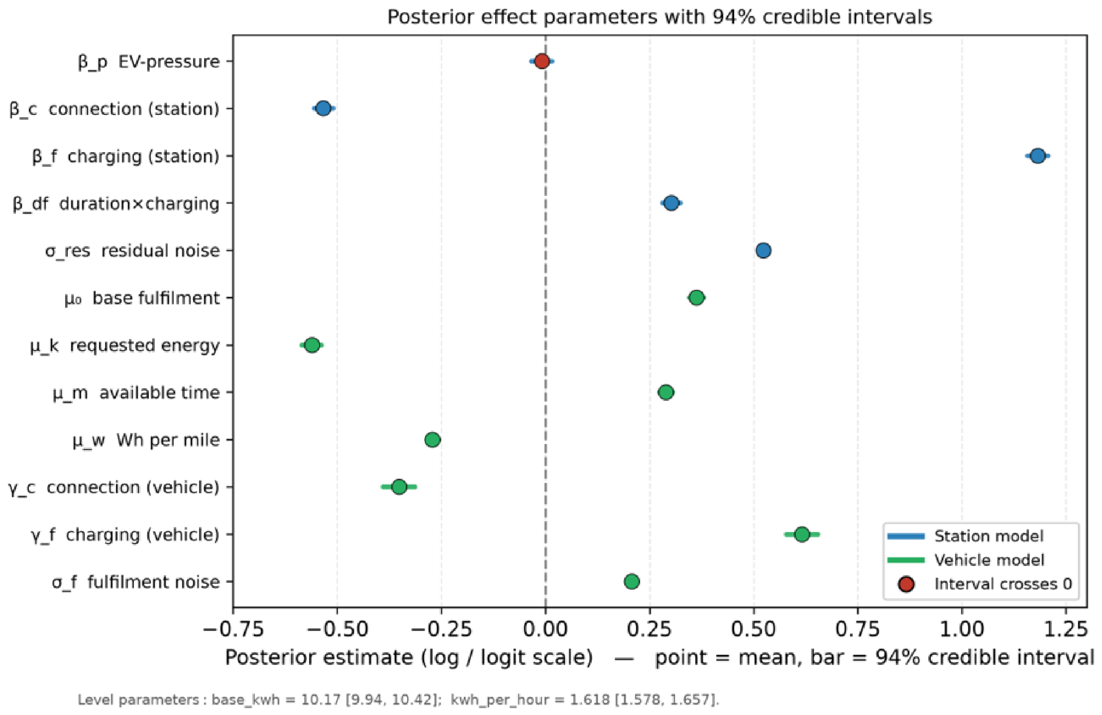
The large sample sizes yield tightly identified posteriors, with narrow credible intervals for almost all parameters. Two features carry physical meaning. First, the credible interval of the EV-pressure effect β_p spans zero ([−0.034, +0.015]), so the instantaneous network load has no statistically resolvable effect on the energy delivered in a session—delivered energy is governed chiefly by dwell time and charging type. Second, the charging-type effect is strongly positive and well separated from zero (β_f: [1.157, 1.207]; γ_f: [0.578, 0.654]), so fast sessions deliver substantially more energy and achieve higher fulfilment. Because inference returns full posterior distributions rather than point estimates, this uncertainty can be propagated into the simulator, and the reported intervals were reproduced from the published code, which recovers the deployed posterior means to within Monte Carlo error.

Both fitted models were serialised and stored so that they can be reused by the simulator without repeating the (computationally expensive) MCMC inference. Crucially, the models are not tied to a specific physical station: partial pooling yields a generic station and vehicle model that can be transferred to new, simulated environments—a prerequisite for using the tool as a planning instrument for networks that do not yet exist.

The hierarchical structure of the station model is shown in Figure 1.

The posterior effect parameters of both models, together with their 94% credible intervals, are summarised in the forest plot of Figure 2. The large sample sizes make the intervals very narrow, so most effects are sharply resolved; the only exception is the EV-pressure effect β_p, whose interval straddles zero (highlighted), showing that instantaneous network load does not measurably affect the energy delivered in a session.

3.4. Model Validation

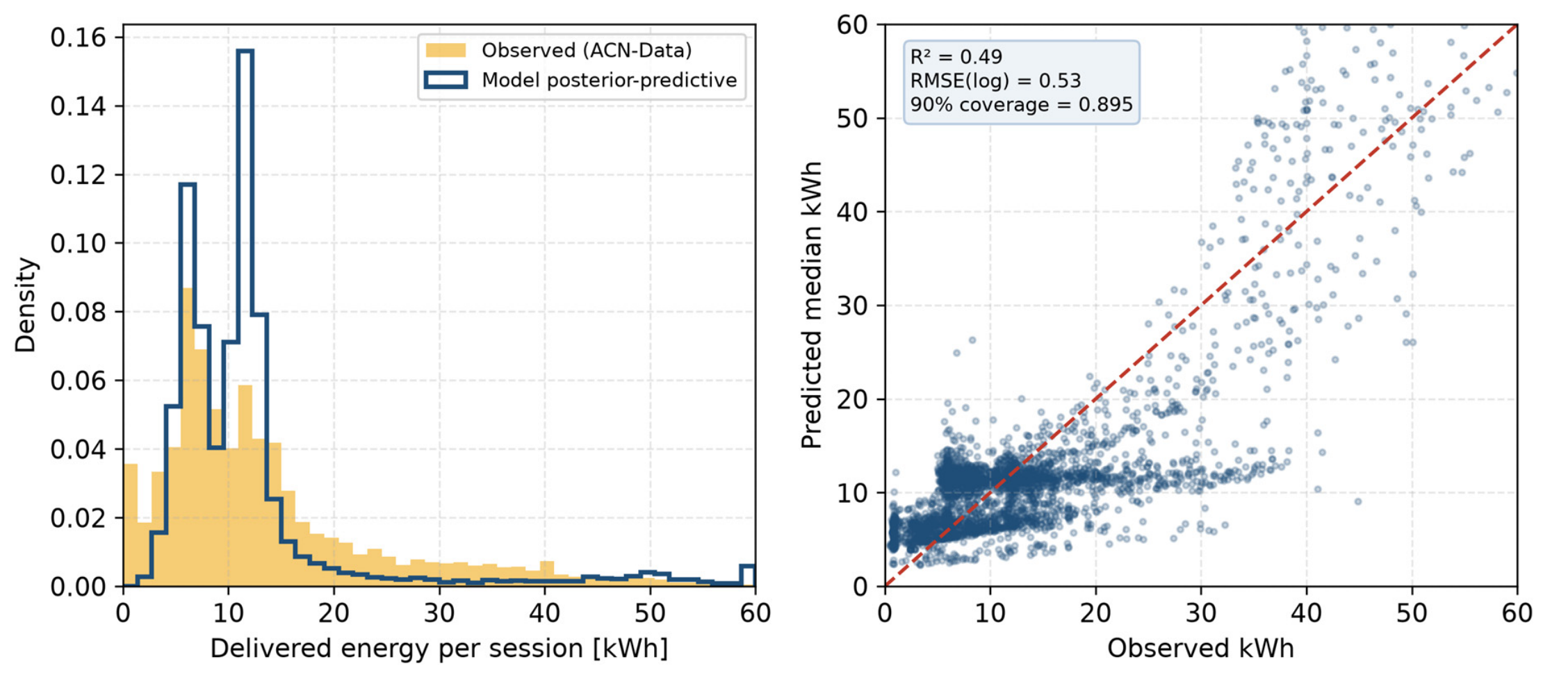
Before the fitted models drove the simulator, their predictive adequacy was checked against the data with an in-sample posterior-predictive check. For every observed session the station model’s posterior predictive distribution of delivered energy was compared with the recorded value. The model is well calibrated: on the log-energy scale it attains a root-mean-square error of 0.52 and an R² of 0.52, and—most importantly for an uncertainty-aware tool—its 90% posterior-predictive interval contains 89.9% of the observations and its 50% interval 54.5%, so empirical coverage is close to the nominal level, with the central interval slightly conservative. The predicted median delivered energy (10.3 kWh) is close to the observed median (10.6 kWh), and the predictive and empirical energy distributions overlap closely (Figure 3). The probabilistic model therefore reproduces both the central tendency and the dispersion of real charging behaviour, and the uncertainty it propagates into the simulation is quantitatively trustworthy rather than nominal.

These two properties answer different questions and should be read separately. The coverage statistics say that the model’s uncertainty is honest: when it declares a 90% predictive interval, very close to 90% of observations fall inside it. That is the property which matters when the fitted posterior is used to drive a stochastic simulation, because it is the width of the distribution, not the location of its centre, that propagates into the queueing behaviour of the network. The R² of 0.52 and the log-scale RMSE of 0.52 describe something quite different—the sharpness of a single point prediction—and they are no better than moderate. Session-level energy is intrinsically noisy, since two vehicles connected for the same time at the same station may request very different amounts of charge, and just under half of the session-to-session variance is not recoverable from dwell time, charging type and connection type. The model is therefore well calibrated but only moderately sharp, and it is presented as such: it is a sound instrument for propagating realistic variability into a network-level simulation, and it is not a precise predictor of any individual charging session.

3.4.1. Generalisation to Unseen Stations

The check above establishes calibration on the data to which the model was fitted. It does not establish that the model transfers to stations it has never seen, which is precisely the situation of a planner sizing a network that does not yet exist. The validation was therefore repeated out of sample. Ten of the 52 stations were held out at random; the model was re-fitted to the remaining 42 stations (11,152 sessions); and the 2542 held-out sessions were then predicted as if they belonged to new sites, with the station-level parameters drawn from the fitted population distribution rather than estimated from the test data. Point accuracy degrades only mildly relative to the in-sample fit—log-scale RMSE 0.54 against 0.52, R² 0.44 against 0.52—and, more importantly for this application, calibration survives the transfer: the 90% predictive interval contains 90.4% of the held-out observations. The partial-pooling structure therefore extrapolates to unobserved stations with uncertainty that remains trustworthy, which is the property the planning use-case depends on.

3.4.2. Comparison with Deterministic and Pooled Alternatives

To place this performance in context, the same held-out sessions were predicted with two simpler models fitted to the same training data: a deterministic global mean, which represents the fixed-average assumption criticised in Section 1, and a pooled ordinary-least-squares regression on the same covariates, which represents complete pooling without any station hierarchy.

Table 3. Predictive performance on 2542 sessions from 10 held-out stations not seen during fitting. All models were trained on the same 11,152 sessions from the remaining 42 stations.

Model	Log-Scale RMSE	R2	90% Interval Coverage
Global mean (deterministic)	0.729	−0.005	not available
Pooled OLS (complete pooling)	0.542	0.445	not available
Hierarchical Bayesian model (this work)	0.543	0.443	0.904

reports the comparison.

The comparison is informative precisely because it is not uniformly flattering. Against the deterministic baseline the improvement is decisive: a fixed average explains essentially none of the variance in held-out sessions (R² ≈ 0), whereas both regression-based models explain about 44% of it, which quantifies the objection to deterministic sizing rules raised in Section 1. Against pooled ordinary least squares, however, the hierarchical model is statistically indistinguishable in point accuracy—0.543 against 0.542 in RMSE—and this is the expected outcome rather than a disappointing one. For a station that has never been observed there is by construction no station-specific information to exploit, so the hierarchy can only fall back on the population distribution, which is close to what complete pooling estimates directly. The added value of the Bayesian formulation therefore does not lie in sharper point prediction at new sites. It lies in the fact that the model returns a calibrated predictive distribution at all—the least-squares fit yields a point estimate with no honest interval attached—and in the fact that, for stations which are observed, partial pooling stabilises station-level estimates without erasing their individual character (Section 2.4). Objective (v) of Section 1 should be read in this light: the demonstrated advantage of the proposed approach over deterministic and pooled alternatives is quantified and validated uncertainty, not point-forecast accuracy.

3.4.3. Likelihood Choice for the Bounded Fulfilment Ratio

The fulfilment ratio is a proportion, and Section 3.3 noted that a normal likelihood centred on a sigmoid mean does not respect that bound. The magnitude of the problem was quantified and an alternative was fitted. Under the published specification, 6.06% of the posterior predictive mass falls outside the admissible interval [0, 1]—not a negligible tail, but roughly one draw in sixteen. The model was therefore refitted with a Beta likelihood, Beta(μφ, (1 − μ)φ), retaining the same linear predictor and the same sigmoid link so that only the observation model changes.

Table 4. Comparison of observation models for the vehicle fulfilment ratio, fitted to the same 16,468 user sessions with identical linear predictors. Expected log predictive density is estimated by leave-one-out cross-validation (higher is better).

Observation Model	RMSE	90% Coverage	Predictive Mass Outside [0, 1]	ELPD (LOO)
Normal(sigmoid(η), σ)—as published	0.207	0.910	6.06%	2538 ± 85
Beta(μφ, (1 − μ)φ)—refitted	0.208	0.902	0.00%	4276 ± 73

compares the two.

The Beta specification is decisively better on predictive density—the difference in expected log predictive density is about 1740, an order of magnitude larger than its own standard error—and it respects the support of the response by construction, so no truncation is required at either fitting or simulation time. Its calibration is also marginally closer to nominal (0.902 against 0.910 for a nominal 0.90). Point accuracy is unchanged (RMSE 0.208 against 0.207), which is expected: both models share the same mean function, and they differ only in how they distribute probability around it. The estimated effects keep their signs, their ordering and their significance, The slope effects are attenuated by 6–22% (for example the requested-energy effect moves from −0.561 to −0.436) while the intercept moves in the opposite direction, rising by 11%, because the Beta model attributes to skewness what the normal model had to absorb into a symmetric residual. Substantively, therefore, nothing in Section 4 and Section 5 changes: the fulfilment model enters the simulator only through the energy actually delivered in a session and plays no part in the assignment logic, so the service success rate and the waiting time—the two criteria carried into the decision analysis—are unaffected. The Beta form is nevertheless the correct specification for a bounded response and is adopted here.

3.5. Agent-Based Discrete-Event Simulator

The simulator is implemented in an object-oriented style and reproduces the operation of a charging network over 24 h in discrete 5 min steps. Two classes carry the state: ChargingStation, holding a fixed number of slots and their occupancy, and Vehicle, holding the arrival time and the sampled energy request, available time and consumption drawn from the vehicle model. On assignment, the energy delivered in a session is predicted from the station model as a function of the (randomly drawn) session duration, charging type, connection type and EV pressure, and is capped by the requested energy times the fulfilment ratio predicted by the vehicle model.

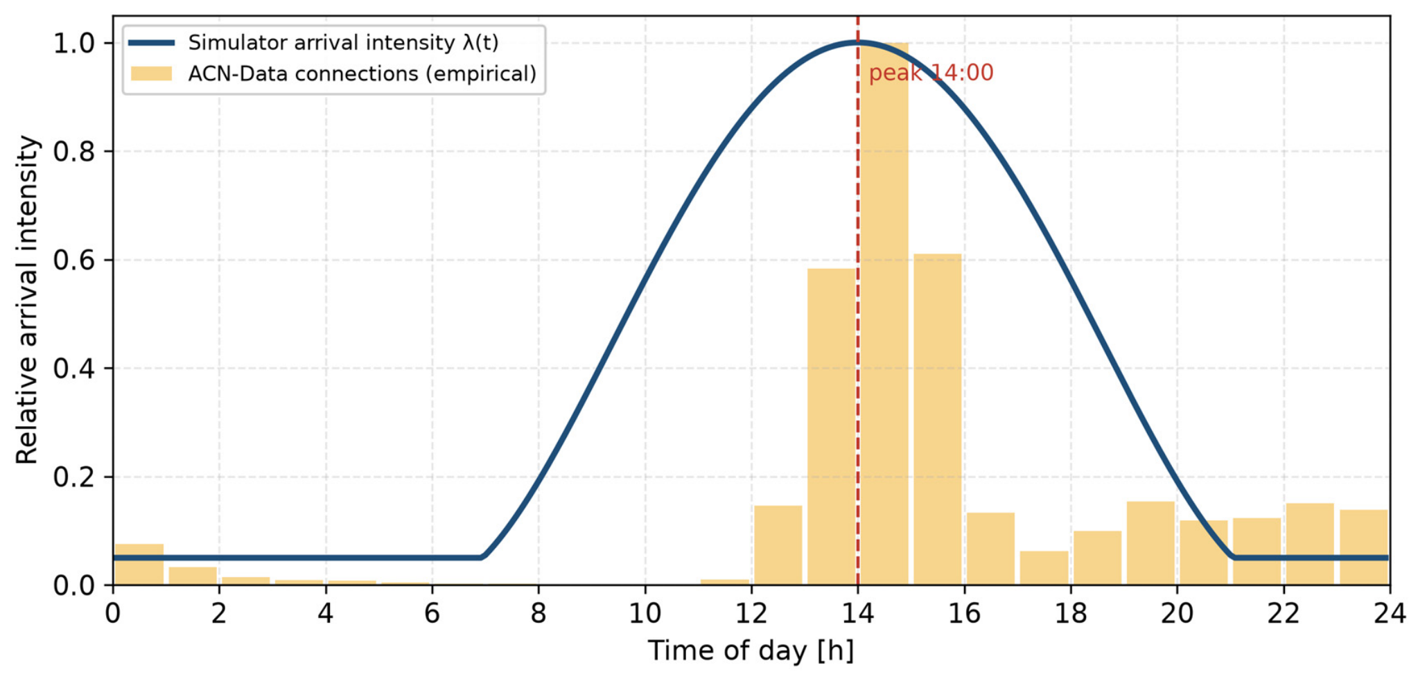
Arrival times for the fixed fleet are drawn with a time-varying intensity, modelled through a custom density function that concentrates arrivals around a configurable peak hour with a specified spread:

$$\lambda (t)\propto {[1-{\left(\frac{\delta (t)}{s}\right)}^2]}^2 \mathrm{for} \delta (t)<s, \lambda (t)=0.05 \mathrm{otherwise}$$

where δ(t) is the circular distance (in minutes) from the peak and s is the spread. The peak hour is not assumed but taken from the data: the connection times in ACN-Data concentrate strongly in the early afternoon and peak at 14:00, which the intensity profile reproduces (Figure 4). Session dwell times are drawn from a log-normal distribution fitted to the observed durations (μ_log = 1.81, σ_log = 0.67; median 6.1 h, mean 7.6 h), so that they are positive and right-skewed; Section 5.3 compares this fitted distribution with the observed durations; the same draw sets both the slot-occupancy window and the duration covariate of the energy model. A vehicle’s charging type (fast/slow) and connection type (charging/discharging) are sampled from their empirical proportions in the dataset (19.8% fast, 16.1% discharging) rather than from arbitrary constants.

The main simulation loop, at each time step, releases vehicles whose sessions have ended, appends newly arrived vehicles to a waiting queue, and assigns queued vehicles to randomly ordered stations with free slots; a vehicle that waits longer than two hours without assignment is recorded as unserved. The total instantaneous load of the network is the sum of the powers of all active sessions,

$$P(t)={\sum }_{i=1}^{n(t)}{P}_i(t)$$

where n(t) is the number of active sessions and P_i(t) the power of session i. Each session is assigned a constant average power—its delivered energy divided by its dwell time—so P(t) is a session-averaged approximation of the instantaneous load rather than a within-session power profile. To stabilise the reported indicators against sampling noise, the Monte Carlo approach of repeated simulation is used. The simulator writes a text report, per-vehicle and per-station CSV files, and figures of the charging-power curve and the served/unserved distribution.

3.6. Simulation Scenarios

Nine scenarios were evaluated for a fixed fleet of 500 vehicles over 24 h with the demand peak at 14:00. Starting from an initial network of 15 stations with 2 slots each, the number of stations was increased to 45 and the number of slots per station to 4, giving a total capacity ranging from 30 to 180 charging slots. Each scenario was assessed by the service success rate (share of vehicles charged) and the mean waiting time, computed over all vehicles with unserved vehicles censored at the two-hour abandonment threshold. To reduce Monte Carlo noise, each scenario was repeated over thirty random seeds and the reported values are the run means; the sensitivity analyses of Section 5.5 and the spatial comparison of Section 5.7 use ten seeds per configuration, and the load ensembles of Section 5.5.1 use twenty.

4. Results

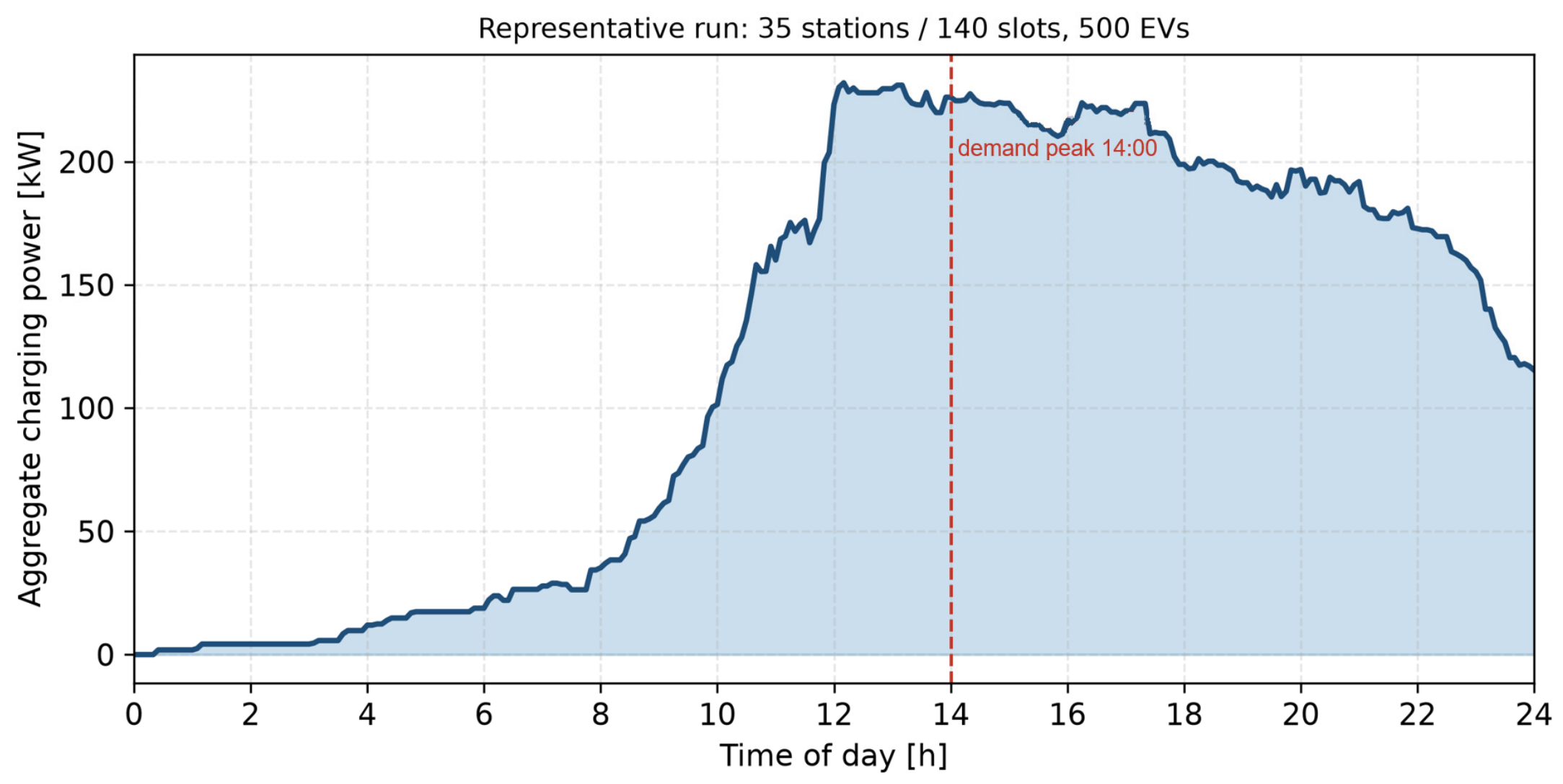
Each of the nine scenarios simulated 24 h of operation for 500 vehicles, progressively increasing the number of stations and slots. Figure 5 shows a representative aggregate charging-power curve (35 stations, 140 slots): the network load tracks the afternoon arrival peak and stays elevated into the evening as long-dwell sessions continue, so the simulator produces a realistic diurnal demand shape rather than a constant load.

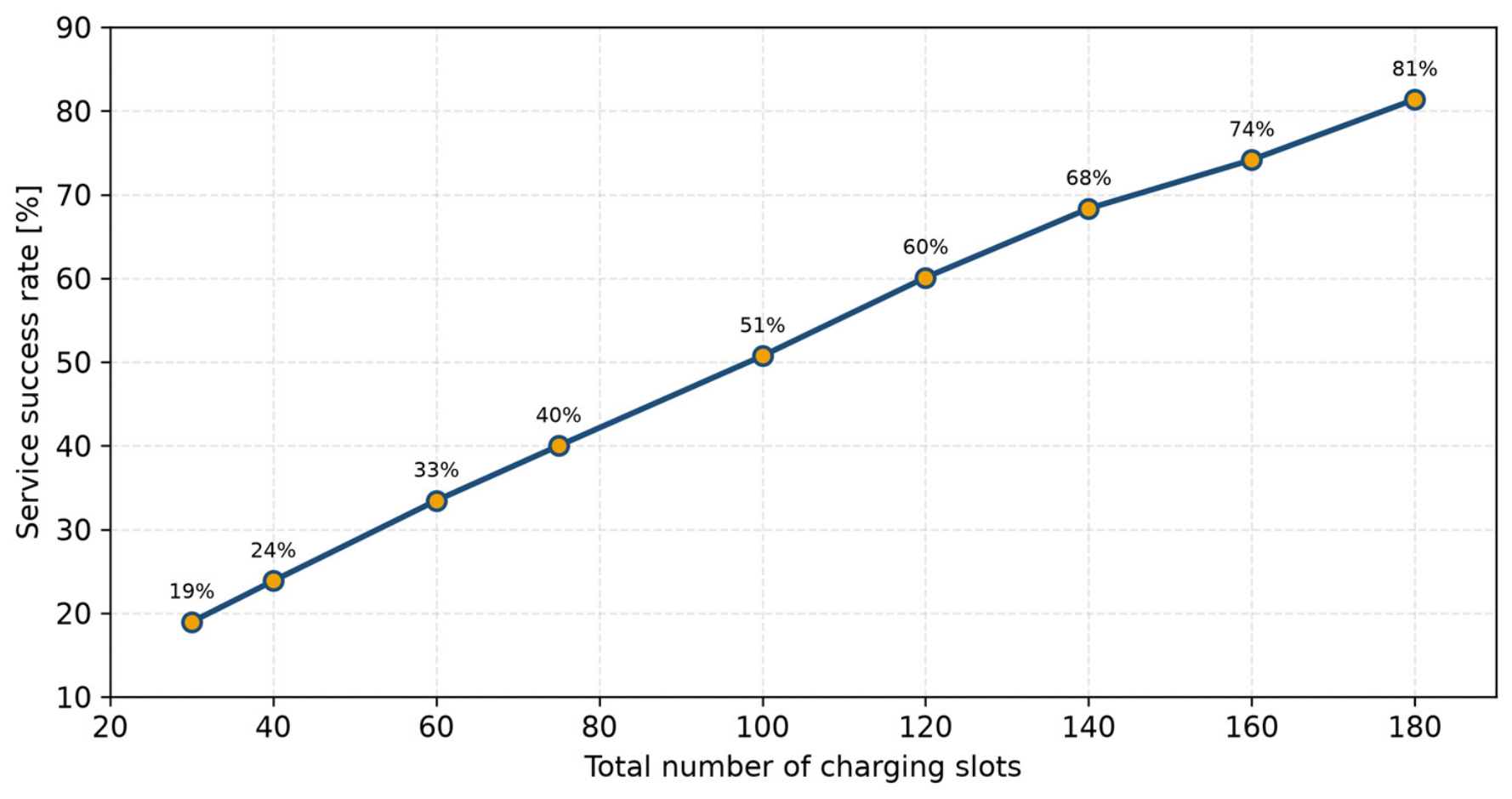
The central result is a monotonic but strongly concave improvement of service quality with capacity, summarised in

Table 5. Results of the nine simulation scenarios (500 vehicles, 24 h, demand peak 14:00; Monte Carlo means over thirty seeds).

Scenario	Stations	Slots (Total)	Service Success Rate	System State
1	15	30	18.8%	Severe capacity shortage
2	20	40	24.0%	Heavily saturated
3	20	60	34.1%	Saturated at peak
4	25	75	41.0%	Persistent peak overload
5	25	100	51.5%	About half served
6	30	120	59.5%	Improving
7	35	140	67.4%	Good; peak still binds
8	40	160	75.2%	High but not saturated
9	45	180	81.4%	Best tested; peak-limited

and Figure 6. With only 30 slots (15 stations) the network served just 19% of the fleet, indicating a severe capacity shortage. Adding capacity raised the service rate steadily—24% at 40 slots, 34% at 60, 52% at 100, and 67% at 140—but even the largest network tested (180 slots, 45 stations) served only 81% of the fleet, and full service was not reached within the studied range for this 500-vehicle fleet. Section 5.5 shows that this last statement is fleet-specific rather than a property of the infrastructure: a 300-vehicle fleet is served completely within the same capacity range, whereas a 1000-vehicle fleet reaches only 47%. The reason is the long dwell time characteristic of workplace charging: with an empirical median session of 8.4 h and a mean of 7.2 h, a slot turns over only a few times per day, so a 500-vehicle fleet concentrated around the afternoon peak saturates the available slots regardless of daily energy headroom. In parallel, the mean waiting time (over all vehicles, unserved censored at the two-hour threshold) fell from about 110 min at 30 slots to about 60 min at 180 slots.

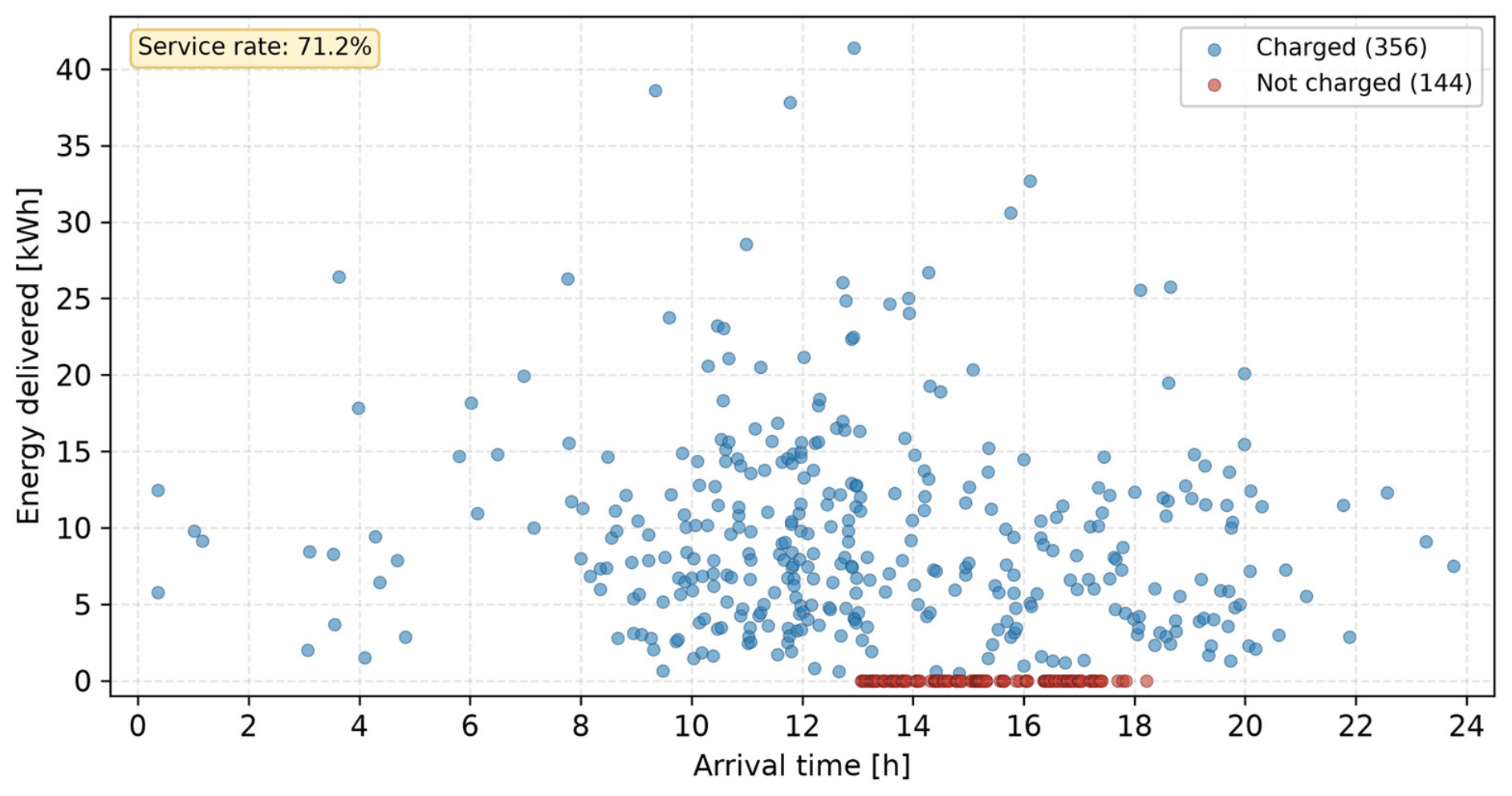
The distribution of served and unserved vehicles for a representative configuration is shown in Figure 7. Unserved vehicles concentrate among those arriving during the demand peak, when all slots are occupied and the waiting queue exceeds the two-hour tolerance, whereas vehicles arriving in the low-demand night and morning hours are almost always served. The binding constraint is therefore peak-hour concurrency rather than daily energy volume, and the simulator captures the queue dynamics of a charging network under stress.

Overall, the simulations show that an insufficient number of charging points leads to full occupation of the network during the peak, high waiting times and many unserved vehicles, and that these effects recede progressively—with diminishing marginal returns—as capacity grows. Because dwell times are long, capacity rather than daily energy is the binding constraint, and even substantial over-provisioning within the tested range does not guarantee full service.

5. Discussion

5.1. Interpretation and Implications for Capacity Planning

Figure 6 carries the central planning message. Service quality improves with capacity but with sharply diminishing marginal returns, and—because long dwell times cap slot turnover—does not reach full service within the tested range. Below a moderate capacity the network is dominated by peak-hour saturation; across an intermediate range each added increment of capacity yields a large improvement; and towards the upper end the marginal gain per added slot falls. The tool’s value for a planner is to locate this concave trade-off for a given fleet and demand shape and to size the network where service quality is balanced against capital cost, avoiding both under-provisioning (long queues, unserved drivers) and over-provisioning (idle chargers). It also makes explicit that, for long-dwell workplace charging, raising raw slot count has limits: beyond a point, demand-side measures that improve slot turnover are more effective than adding hardware.

Because the binding constraint is peak-hour concurrency rather than total daily energy (Figure 7), the results also motivate demand-side measures as an alternative to pure capacity expansion. Shifting or spreading arrivals away from the afternoon peak—through pricing, smart charging or workplace-charging incentives—would raise the effective service rate at fixed capacity, a lever that the same simulation framework can evaluate by reshaping the arrival-intensity function. This connects the present tool to the broader literature on smart charging and grid-impact mitigation, where coordinating charging with network constraints is repeatedly found to be more cost-effective than reinforcement alone [22,23,24,25], and to work coupling charging with local photovoltaic generation for greater self-consumption and sustainability [26].

5.2. Evaluation of the Modelling Approach

The hierarchical Bayesian model performed as intended and, unlike the original design, is now validated (Section 3.4). Partial pooling stabilised the station-level estimates during fitting, and the model captured the relationship between session duration and delivered energy, the strong effect of charging type on station output, and the difference between charging and discharging modes; it also found that the network-load proxy (EV pressure) has no resolvable effect on delivered energy (β_p ≈ 0). Using MCMC inference rather than point estimation produced full posterior distributions, so that system uncertainty could be propagated into the simulation. The simulator then uses the pooled generic-station parameters rather than individual station estimates—appropriate for planning networks whose stations do not yet exist, though at the cost of not exploiting station-to-station heterogeneity, which is a deliberate simplification rather than a use of the full hierarchy at run time. These properties align the approach with recent hierarchical and probabilistic forecasting work that emphasises uncertainty quantification and cross-scale consistency [5,6,7,8], and with the open-data ethos that underpins reproducible EV-charging research [2,20].

The simulator realistically reproduced the operation of the network over the full 24 h horizon: generated arrivals created natural daytime peaks, the assignment algorithm used the available slots efficiently and distributed load across stations, and the monitored indicators—served and unserved counts, mean waiting time, delivered energy, occupancy and the network power curve—behaved as expected, with high service and low waiting at light load and rising unserved counts under stress. The combination of a hierarchical Bayesian behaviour model with a discrete-event simulation therefore constitutes a coherent and practically useful approach to modelling and analysing charging infrastructure.

5.3. Advantages and Limitations

The main advantages of the implemented system are its use of real data from the ACN-Data dataset, its probabilistic foundation validated in and out of sample (Section 3.4), its ability to model system uncertainty, and the flexibility of the simulation environment. The limitations are set out below in the order in which they would affect a reader’s use of the results. Several of them were identified by re-examining the implementation against the reported values while preparing the reproduction package, and they are stated with their magnitudes rather than in general terms, because a limitation whose size is unknown cannot be worked around. Finally, the reported figures are Monte Carlo means over thirty seeds for the main scenarios and ten or twenty for the sensitivity and ensemble analyses; individual runs carry sampling variability, so the values should be read as estimates rather than exact quantities.

Delivered energy is generated by the station model alone. An earlier version of the simulator additionally capped each session at the product of the requested energy and the fitted fulfilment ratio; because that ratio is itself defined as delivered energy divided by requested energy, the cap took the minimum of two estimates of the same quantity and biased delivered energy downward by about a third. The station model is now used on its own and the fulfilment ratio is reported as a diagnostic rather than used to generate energy. A residual bias remains in the opposite direction: simulated sessions average about 16 kWh against 13.7 kWh in the fitting corpus, roughly 20% high, because the simulator draws dwell time, requested energy and the remaining covariates from their marginal distributions and so does not reproduce the correlations between them that are present in real sessions. The median, which is less sensitive to that effect, is close to the observed value. Load and energy figures should therefore be read with a tolerance of roughly this size.

The load model is a session average, not an instantaneous profile. Each session is assigned a constant power equal to its delivered energy divided by its dwell time, so a vehicle that charges for three hours and then sits connected for five is represented as drawing a low power throughout. Because ACN-Data records the moment charging completes, the size of this approximation is measurable: actual charging power averages about 3.5 kW against 2.2 kW for the session-averaged proxy, and the median session is idle for roughly 40% of its dwell. The peak loads reported here are correspondingly conservative—the figure of roughly 2.4 to 2.7 kW per installed slot is a diversity-adjusted average rather than a connected rating, and it should not be compared directly with the 3.7–22 kW ratings of the AC hardware described in Section 1. A network designed on these figures would be under-dimensioned; a design study would need the within-session power profile and a high quantile of the load rather than its mean.

Three covariates are of undocumented provenance. The EV-pressure estimate, the connection type and the charging type are present in the dataset file used here but are not part of the public ACN-Data schema, and the rule by which they were derived is not recorded. Two of them carry the largest effects in Table 1. This matters for their interpretation. The EV-pressure variable is constant within every station in the sample, so it is exactly collinear with the station intercepts and is identified only through the partial-pooling prior; the near-zero posterior reported in Section 3.2 therefore indicates that the effect of network load is not identifiable in these data, and not that network load has no effect. Similarly, no session in the corpus exceeds 9 kW, so the sessions labelled fast are not direct-current charging events in the sense of Section 1, and the 20% direct-current share assumed in the cost model of Section 5.6—which was aligned with the observed share of fast sessions—conflates a share of sessions with a share of installed slots and should not be read as a statement about hardware. Reproducing this study from the public ACN-Data release alone would require these three fields to be reconstructed, and the derivation is not available to us.

The hierarchy is fitted but not exercised at run time. Partial pooling stabilises the station-level estimates during inference, and the out-of-sample test of Section 3.4.1 shows that the fitted population distribution transfers to unseen stations. The simulator, however, is parameterised with the pooled generic-station values and does not draw a distinct parameter set for each simulated station, so every station in a simulated network behaves identically. Because the between-station standard deviations are small relative to the residual scale—0.079 and 0.081 against 0.523, about 2% of the residual variance—the practical consequence is limited, and it is also the reason the hierarchical model ties with a pooled regression on held-out stations in Table 3. It does mean, however, that the station-to-station heterogeneity the hierarchy estimates is not present in the simulated networks, and that utilisation imbalance in Section 5.7 arises from geography alone.

The dwell-time distribution is fitted by a family that does not match its shape. The observed durations have a median of 8.4 h above a mean of 7.2 h, that is a left-skewed, workday-shaped distribution with a tail of short sessions. The log-normal fitted in Section 3.5 is right-skewed by construction, has a median of 6.1 h and a standard deviation of 5.7 h against 3.3 h in the data, and is rejected by a Kolmogorov–Smirnov test. Since slot turnover is the mechanism behind the central finding, this misfit matters: resampling the observed durations empirically instead lowers the service rate at the largest network by roughly four percentage points. The qualitative conclusion—that concurrency rather than daily energy binds—is unchanged, but the absolute service rates would shift, and an empirical resampling of dwell times is the second item of future work. Where the text quotes a median dwell of about six hours it refers to the fitted distribution; the empirical median is 8.4 h, as stated in Section 1.

The scenario design constrains what the decision analysis can find. The nine configurations increase the number of stations and the number of slots per station together, from two slots per station in the smallest to four in the largest, so station count and station size cannot be separated—which is precisely the trade-off that per-station fixed costs in Section 5.6 and station siting in Section 5.7 turn on. The service–capacity relationship over this range is also close to linear rather than strongly concave, with a straight line accounting for almost all of the variation, so the language of a knee and of sharply diminishing returns should be read as describing the expected long-run behaviour of such a network rather than a feature resolved within the tested range. Every optimum reported here lies at an end of the tested set, so the analysis brackets the compromise region rather than locating an interior optimum; extending the range upward would be required to do the latter.

Three narrower caveats complete the list. The service rate and the waiting time are not independent criteria, since the waiting time is computed over all vehicles with unserved vehicles censored at the abandonment threshold and is therefore largely determined by the service rate; the same objection the present study raises against splitting cost into two collinear criteria in Section 5.6 applies, to a lesser degree, to this pair. And the 16,468 user requests are not independent observations, being on average 1.2 requests recorded within each of the 13,694 sessions and sharing a delivered energy, so the credible intervals of Table 2 are narrower than an independent sample of that size would give.

5.4. Multi-Criteria Selection of the Optimal Configuration

The simulation produces a full performance profile for every candidate configuration, which turns network sizing into a concrete MCDM problem of the kind formalised in Section 2.5. Three criteria were used: the service success rate S (benefit), the mean waiting time W (cost), and the installed capacity C, taken as the total number of charging slots and used as a proxy for capital cost (cost). The criterion values, obtained as Monte Carlo means over thirty independent simulation runs per configuration—reproducing the trend of Table 5—are listed in

Table 6. Multi-criteria decision matrix (Monte Carlo means over thirty runs) and the TOPSIS closeness coefficient under the balanced weighting.

Scenario	Stations	Slots (C)	Service Rate S [%]	Waiting Time W [min]	TOPSIS CC (Balanced)
1	15	30	18.8	110.2	0.407
2	20	40	24.0	107.3	0.412
3	20	60	34.1	101.5	0.438
4	25	75	41.0	96.9	0.467
5	25	100	51.5	89.3	0.524
6	30	120	59.5	82.8	0.565
7	35	140	67.4	76.1	0.591
8	40	160	75.2	68.9	0.600
9	45	180	81.4	61.5	0.593

. TOPSIS was then applied under three weightings of (S, W, C): a balanced profile (0.50, 0.20, 0.30), a service-priority profile (0.70, 0.15, 0.15) and a cost-priority profile (0.30, 0.15, 0.55).

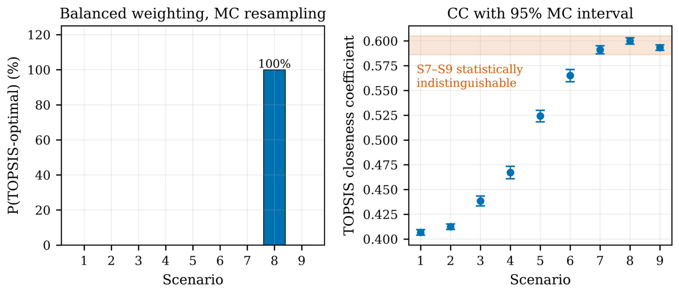
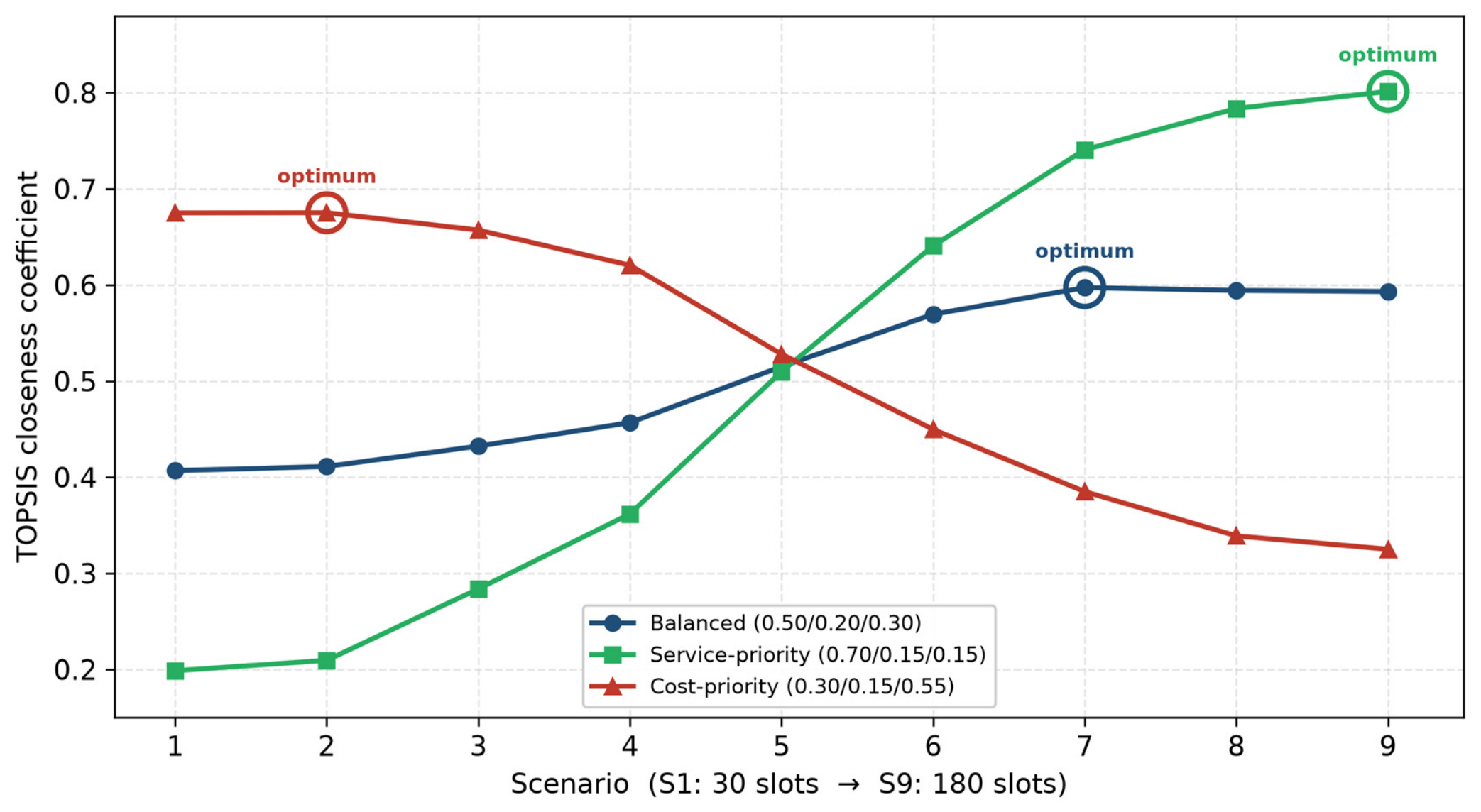
The resulting closeness coefficients are shown in Figure 8, and the ranking depends strongly on the decision-maker’s priorities. Under the cost-priority weighting the optimum is Scenario 2 (40 slots), which accepts a low service rate for minimal investment. Under the service-priority weighting it is Scenario 9 (180 slots), the largest network tested, because service does not saturate within the studied range and so more capacity always helps. Under the balanced weighting the closeness coefficient peaks at Scenario 8 (40 stations, 160 slots, ≈75% service) with 0.600, ahead of Scenario 9 by 0.007 and Scenario 7 by 0.009. Those margins are small, and whether they survive the Monte Carlo uncertainty of the simulation outputs is a question that has to be answered rather than assumed; Section Robustness of the Ranking to Simulation and Weight Uncertainty does so. The balanced optimum sits at the knee of the concave service–capacity curve, where added slots still buy meaningful service but before the marginal return collapses—the diminishing-returns behaviour of Section 5.1, made quantitative and preference-explicit.

This analysis operationalises the decision-support claim of the paper. Rather than defaulting to the capacity that guarantees full service, the coupled pipeline—Bayesian behaviour model → agent-based simulation → MCDM—locates the point on the Pareto front that best matches a stated preference, while the sensitivity of the ranking to the weights (Figure 8) tells the planner how robust that choice is. What the pipeline delivers is therefore a preference-conditional recommendation together with an explicit statement of how firmly it is held—which, as the next subsection shows, is considerably less firmly than a single peak in the closeness coefficient would suggest.

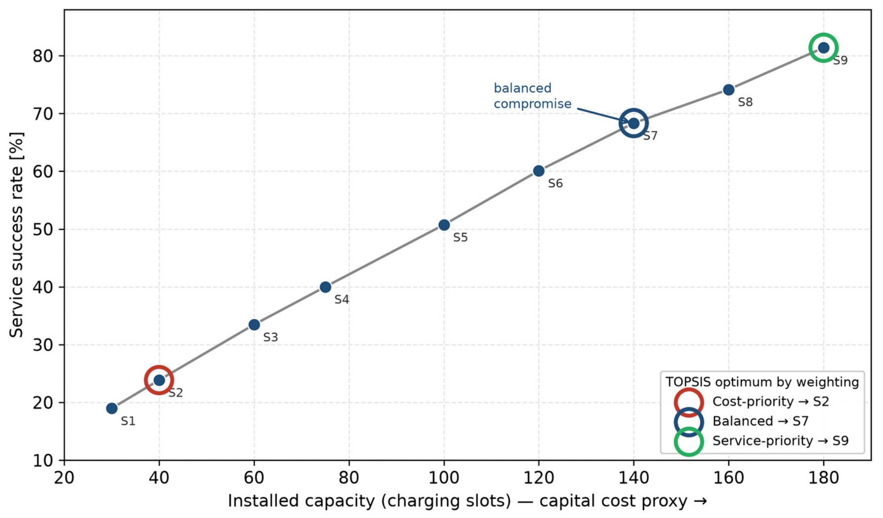
The same trade-off can be read directly from the service–cost frontier in Figure 9. Because the service rate increases monotonically with installed capacity, every configuration is Pareto-non-dominated on the service-versus-cost pair alone, so none can be discarded without an explicit preference statement; the weighting of criteria—and its sensitivity analysis—is therefore indispensable. The three TOPSIS optima mark where each weighting places the compromise along the frontier: cost-priority at the low-capacity end (S2), service-priority at the high-capacity end (S9), and the balanced weighting in the upper-middle of the range (S8, ≈160 slots). As Section Robustness of the Ranking to Simulation and Weight Uncertainty shows, the frontier is sufficiently flat there that S7, S8 and S9 exchange places under modest changes in the weights, so this point should be read as the balanced-weighting member of a compromise band rather than as an optimum independent of preferences.

Robustness of the Ranking to Simulation and Weight Uncertainty

The closeness coefficients of the three highest-ranked configurations differ by less than 0.01, while the criterion values that generate them are themselves Monte Carlo estimates. Whether Scenario 8 can be distinguished from Scenarios 7 and 9 is therefore a question about sampling error, and it can be answered directly. Each configuration was re-simulated over 30 random seeds. Crucially, all configurations share the same seeds, the same fleet and the same arrival draws, so their outcomes are paired: the seed index has to be resampled jointly rather than independently for each configuration, since an independent resampling discards the pairing and inflates the apparent uncertainty of precisely the differences at issue. A paired bootstrap over the seed index was therefore used, recomputing the TOPSIS ranking from the resampled means 5000 times.

Table 7. Monte Carlo variability of the simulation outputs (mean ± standard deviation over 30 independent seeds per configuration) and the resulting probability that each configuration attains the highest TOPSIS closeness coefficient under the balanced weighting, from 5000 resamples.

Scenario	Slots	Service Rate (%)	Waiting Time (min)	Closeness Coeff.	p (Optimal)
1	30	18.8 ± 1.1	110.2 ± 1.0	0.407 ± 0.001	<0.1%
2	40	24.0 ± 1.3	107.3 ± 1.0	0.413 ± 0.001	<0.1%
3	60	34.1 ± 1.9	101.5 ± 1.2	0.438 ± 0.003	<0.1%
4	75	41.0 ± 2.1	96.9 ± 1.0	0.467 ± 0.003	<0.1%
5	100	51.5 ± 2.1	89.3 ± 1.3	0.524 ± 0.003	<0.1%
6	120	59.5 ± 2.0	82.8 ± 1.5	0.565 ± 0.003	<0.1%
7	140	67.4 ± 2.1	76.1 ± 1.7	0.591 ± 0.002	<0.1%
8	160	75.2 ± 2.3	68.9 ± 2.2	0.600 ± 0.002	100.0%
9	180	81.4 ± 2.2	61.5 ± 2.3	0.593 ± 0.001	<0.1%

reports the result.

The per-configuration standard deviations across seeds are 1.1–2.3 percentage points in the service rate and 1.0–2.3 min in the mean waiting time. Once the pairing is respected, however, the uncertainty in the closeness coefficient itself is much smaller than those figures suggest, because the configurations rise and fall together from seed to seed: the bootstrap standard deviation of each coefficient is about 0.002, against gaps of 0.009 between Scenarios 8 and 7 and 0.007 between Scenarios 8 and 9. Scenario 8 attains the highest coefficient in essentially every resample. Under the balanced weighting the optimum is therefore identified sharply, and a network of 40 stations and 160 slots is the compromise this preference structure selects. It is worth being explicit that an earlier, independent resampling of the configurations suggested the opposite—that the three could not be separated—and that this was an artefact of discarding the common random numbers rather than a property of the evidence.

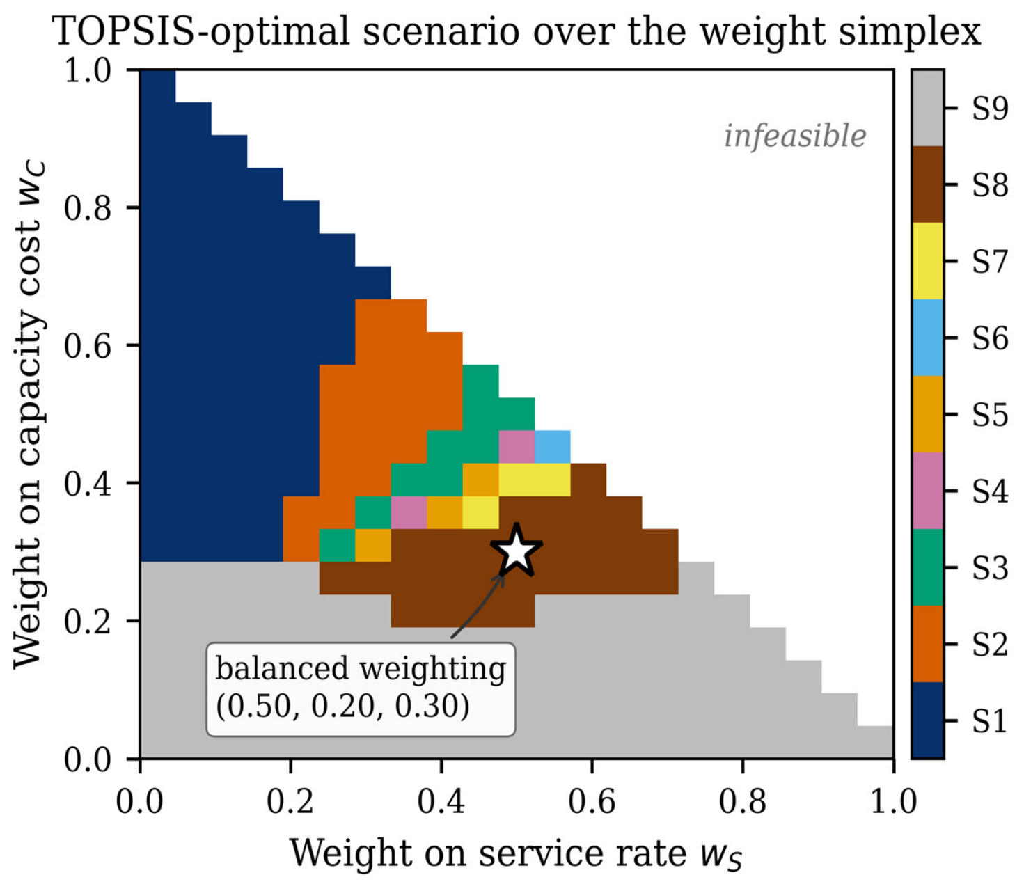
What is fragile is therefore not the estimate but the preference. Figure 10 moves the same question from the simulation outputs to the weights: instead of the three discrete profiles of Table 6, the closeness coefficient was recomputed across the entire weight simplex and the winning configuration recorded at every point. Two large regions dominate—the largest network wherever waiting time carries appreciable weight, at 42% of the simplex, and the smallest wherever capacity cost dominates, at 29%—while Scenario 8, the optimum under the balanced profile, wins only about 12% of it. The balanced weighting sits in a narrow transition band in which the intermediate configurations exchange places over short distances in weight space. The practical reading is the reverse of what the coefficient’s precision might suggest: the analysis pins down the optimum for a given statement of priorities, and a planner who is not confident of those priorities should treat the whole band from Scenario 7 to Scenario 9 as admissible, since a modest change in weights moves the answer across it.

This behaviour is a property of the decision problem rather than a defect of the method. Because the service rate rises with capacity while cost rises with it as well, the alternatives form a smooth and densely populated Pareto front (Figure 9), and on such a front many configurations are near-optimal for neighbouring weight vectors. The lesson for reporting is that simulation uncertainty and preference uncertainty are different things and behave differently: the first can be made small by running more seeds and by exploiting the pairing between configurations, whereas the second cannot be reduced by computation at all. Presenting the coefficient intervals and the weight map together is therefore the appropriate response, and it is the weight map that carries the caveat.

Based on Figure 8, the margin separating Scenarios 7 to 9 under the balanced weighting is within Monte Carlo uncertainty and is assessed in Section Robustness of the Ranking to Simulation and Weight Uncertainty and Figure 11.

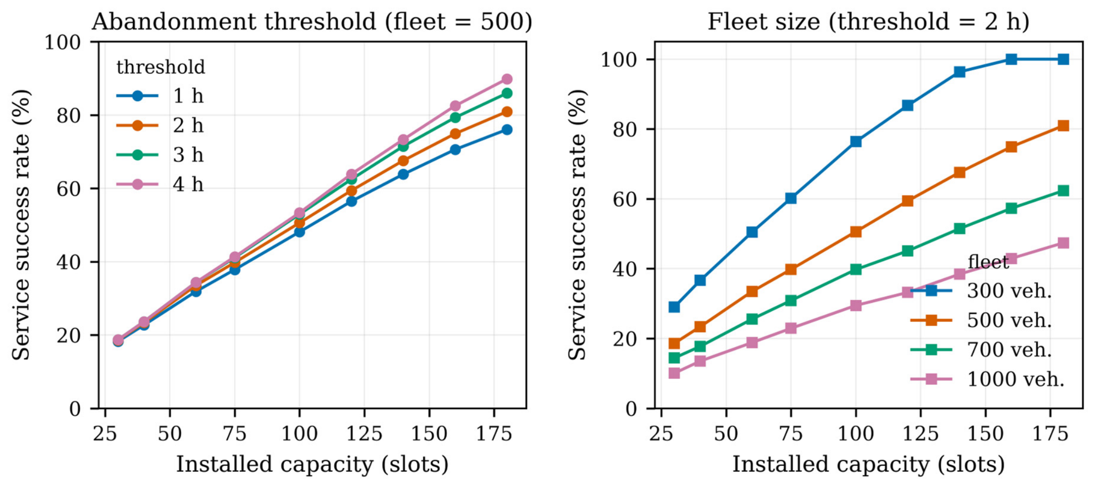
5.5. Sensitivity to the Simulation Assumptions

Two modelling choices exert a strong influence on the reported indicators, and both were varied systematically to establish how far the conclusions depend on them: the two-hour abandonment threshold and the size of the vehicle fleet. Figure 12 summarises the outcome.

The abandonment threshold defines when a waiting vehicle is recorded as unserved and therefore enters both reported indicators directly. Raising it from one hour to four raises the service rate of the largest network from 76.1% to 89.9%, while leaving the smallest network essentially untouched (18.3% against 18.7%). The asymmetry is itself informative: where capacity is severely short, vehicles go unserved however long they are prepared to wait, so the threshold is immaterial; where capacity is close to adequate, the threshold governs how much of the residual queue is eventually absorbed. The headline figure of 81% at 180 slots should accordingly be read as 76–90% across the plausible range of driver patience. What does not change across that range is the shape of the relationship or the conclusion drawn from it: at every threshold tested the service–capacity curve is concave, full service is not attained within the tested range, and peak concurrency rather than daily energy remains the binding constraint. The mean waiting time is more sensitive still, because unserved vehicles are censored at the threshold when the mean is formed; that indicator is best read as a bounded index of congestion rather than as an estimate of the delay an individual driver would experience, and the censoring convention is stated explicitly in Section 3.6 for that reason.

Fleet size qualifies one of the reported conclusions more sharply. The statement that full service is not reached within the tested capacity range holds for the 500-vehicle fleet, but it is not a property of the infrastructure alone. With 300 vehicles the network is already near saturation at Scenario 7 (96.4%) and reaches complete service at 160 slots, whereas with 700 and 1000 vehicles the largest configuration tested serves only 62.3% and 47.4% respectively. The governing quantity is the ratio of vehicles to installed slots together with the dwell-time distribution: the configurations examined here span roughly 1.7 to 33 vehicles per slot, and for the observed workplace dwell times service quality falls away steeply once that ratio rises much above three. The absolute percentages in Table 5 should therefore be read as specific to a 500-vehicle workplace fleet, while the concave, concurrency-limited shape of the response—and the planning logic built on it—is the transferable finding.

5.5.1. Run-to-Run Variability of the Load Profile

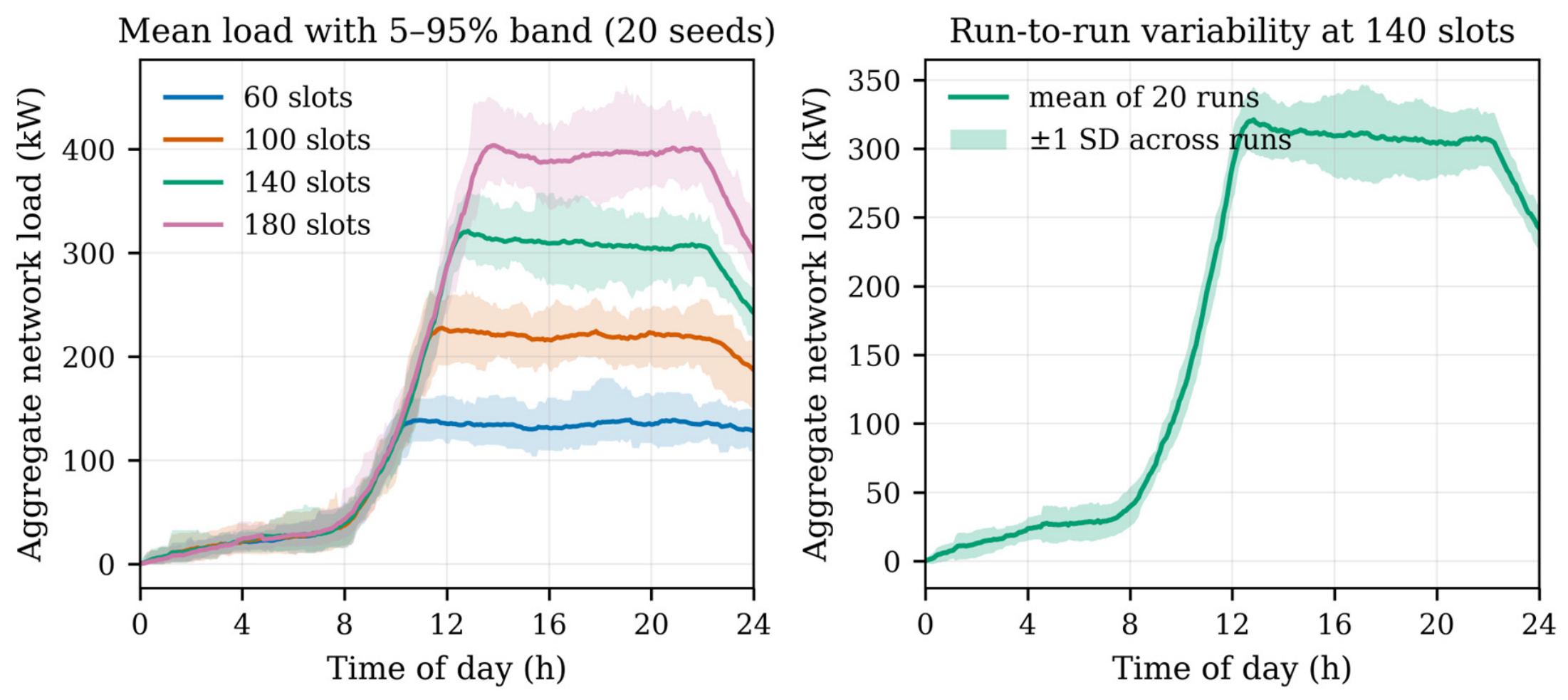
Figure 5 shows the aggregate load of a single representative run, and a single stochastic realisation cannot separate structure from sampling noise. The load profile was therefore recomputed as an ensemble: every configuration was simulated over twenty independent seeds and the mean profile is reported with the band containing the central 90% of runs (Figure 13). The ensemble reveals a load profile that is far flatter than a single run suggests. Once the network fills in the late morning it stays within five per cent of its maximum for between nine and twelve hours of the day, so the diurnal shape is better described as a broad daytime plateau than as a peak: with a median dwell of several hours, sessions started across the whole arrival window overlap for most of the working day. A consequence worth stating is that the time at which the maximum happens to fall is not a meaningful statistic here, because the profile is nearly level over that span and the location of its maximum is dominated by sampling noise. The magnitude, by contrast, is stable and scales almost linearly with installed capacity, from 82 kW at 30 slots to 425 kW at 180, that is between roughly 2.4 and 2.7 kW per installed slot. This is the diversity-adjusted average load per charge point rather than a connected rating, and it remains below the 3.7–22 kW range of the alternating-current hardware described in Section 1 because slots are neither occupied at every moment nor drawing full power throughout a session; Section 5.3 quantifies the second of those effects.

5.5.2. Demand Shifting as an Alternative to Building Capacity

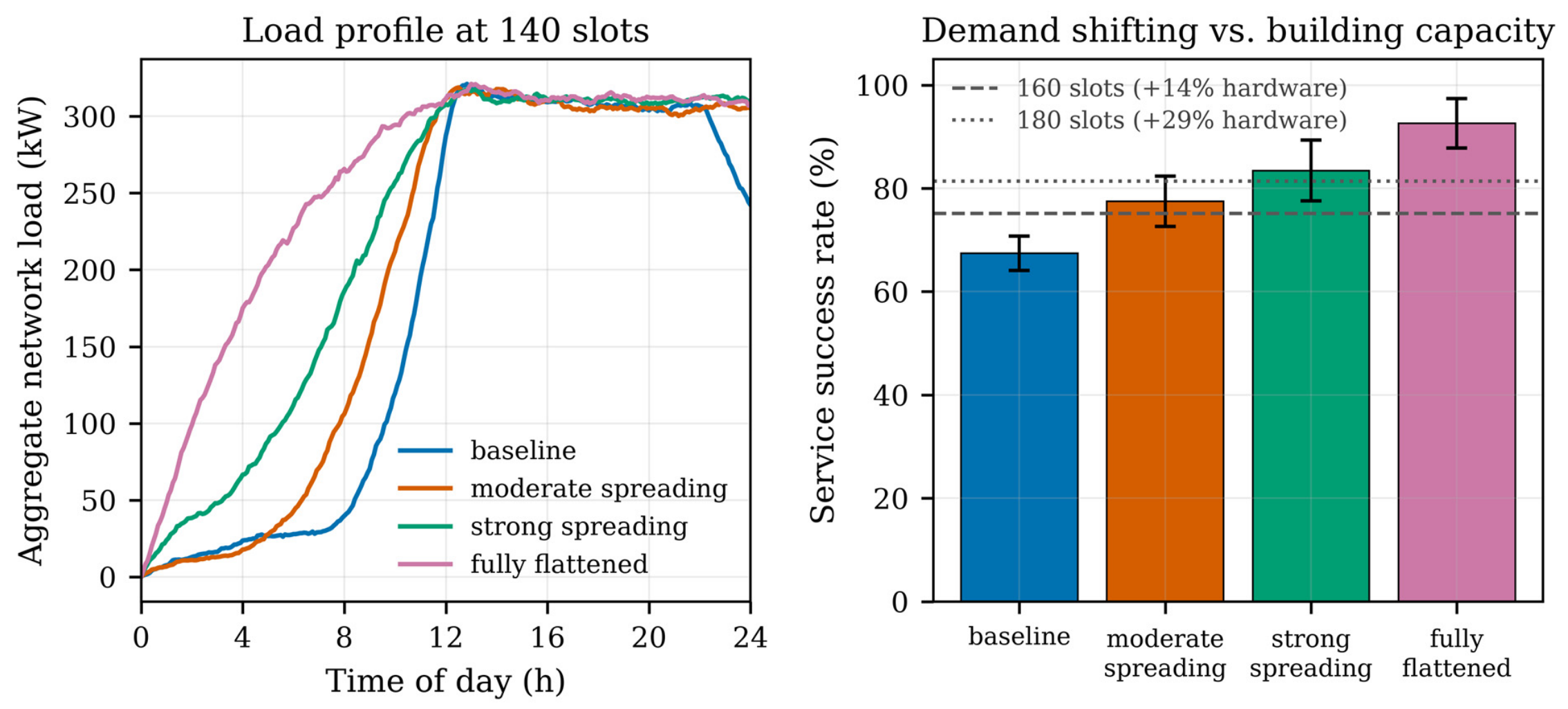
Section 5.1 argued that, because the binding constraint is peak concurrency rather than daily energy, spreading arrivals should raise the service rate at fixed hardware. That argument is testable within the same framework, since the arrival intensity is an explicit input, and it was tested. Holding the network fixed at 140 slots, the arrival profile was progressively flattened by widening the spread of the intensity function from the fitted 8 h to 12 h and 16 h, and finally to a uniform 24 h profile representing complete decoupling of charging from the arrival peak. Figure 14 reports the outcome.

The effect on service is large. At unchanged hardware the service rate rises from 67.4% under the observed profile to 77.5% under moderate spreading, 83.4% under strong spreading and 92.6% under a fully flattened profile, while the mean waiting time falls from 76.0 to 36.8 min. The comparison that matters for a planner is with the cost of achieving the same service by construction: at the observed arrival profile, 160 slots deliver 75.2% and 180 slots deliver 81.4%. Moderate spreading at 140 slots therefore outperforms a 14% capacity expansion, and strong spreading matches a 29% expansion, with no additional chargers. The peak load, however, does not fall: it stays close to 340 kW across all four profiles and if anything rises slightly, because spreading arrivals allows the network to serve more vehicles and the additional energy offsets the smoother arrival pattern. Demand shifting in this setting therefore buys throughput rather than peak reduction, and it does so precisely because the binding constraint is the availability of slot-hours rather than instantaneous power. A grid-connection saving should not be claimed for it; the saving is in chargers that do not have to be built. This is the quantitative form of the sustainability argument in Section 5.8: the embodied material and manufacturing impact of the chargers that are not built is avoided outright. No grid saving accompanies it, as the peak is unchanged, so the benefit is in hardware rather than in connection capacity. The claim also needs bounding. Fully flattening workplace arrivals is not achievable in practice, since arrival times are set by working hours rather than by tariffs; the 12 h and 16 h cases are the policy-relevant ones, and even they assume a price or incentive response strong enough to move a substantial share of users. The framework quantifies what such a response would be worth, and the behavioural model that would predict its size is taken from the literature on time-of-use response [11] rather than estimated here.

5.6. A Segmented Cost Model and the Limits of Criterion Refinement

The decision analysis of Section 5.4 uses the installed slot count as a proxy for cost. That proxy is transparent but crude: it treats every slot as identical, ignores the fixed cost of opening a station at all, and takes no account of operating expenditure. To test whether that simplification matters, the analysis was repeated with a segmented cost model. Capital expenditure is decomposed into a per-station fixed component covering site works, metering and the connection point, a per-slot charger cost that distinguishes alternating-current from direct-current hardware, and a distribution-network reinforcement term proportional to the peak load each configuration actually imposes, taken from the thirty-seed simulations of Table 5. Annual operating expenditure comprises maintenance proportional to installed hardware, a network capacity charge on peak load, and the cost of the energy delivered, which for workplace charging is borne by the operator rather than passed through. Capital and operating expenditure then enter TOPSIS as two separate cost criteria alongside service rate and waiting time, as is standard practice in infrastructure appraisal.

All costs are expressed in relative units, one unit being the installed cost of a single alternating-current slot. Absolute currency values are specific to a country and a year and would date the result; the cost ratios are the transferable part, and they are the only thing the ranking depends on. The baseline assumes a direct-current slot at ten times the cost of an alternating-current slot, a per-station fixed cost of four slot-equivalents, a direct-current share of 20% matching the fast-charging share observed in the data, network reinforcement at 0.08 units per kW of peak load, annual maintenance at 6% of hardware capital, and a capacity charge of 0.02 units per kW per year. Because every one of these figures is an assumption, each was varied over a plausible range individually, and all six were then varied jointly.

Table 8. Segmented cost model in relative units (1 = installed cost of one AC slot), with peak load taken from the thirty-seed simulations of Table 5. CAPEX and annual OPEX enter the decision analysis as separate cost criteria.

Scenario	Stations	Slots	Peak Load (kW)	CAPEX	OPEX per Year
1	15	30	82	151	872
2	20	40	105	200	1085
3	20	60	155	260	1565
4	25	75	191	325	1897
5	25	100	247	400	2375
6	30	120	296	480	2736
7	35	140	337	559	3086
8	40	160	381	638	3460
9	45	180	425	718	3732

gives the baseline result.

Two results follow, and both are cautions about the method rather than findings about the network. Capital and operating expenditure, modelled this way, correlate at 0.996 across the nine configurations. The reason is not the one that might be expected: maintenance and the capacity charge together account for barely 2% of operating expenditure, and the remaining 98% is the cost of the energy actually delivered. Operating expenditure is therefore very nearly a monotone transform of the service rate, with which it correlates at 0.99995—so a criterion entered as a cost is in substance the benefit criterion with its sign reversed, and the aggregation rewards service at a weight of 0.50 while penalising it at 0.10. Entering them as two criteria therefore adds almost no information beyond entering one: it splits a single cost dimension into two near-duplicate columns and, in a weighted aggregation, simply redistributes the weight already assigned to cost. Separating investment from operating cost is worthwhile when the two diverge—for instance when comparing a cheap installation with expensive maintenance against the reverse—but for a homogeneous family of configurations differing only in scale, it does not. This is reported because the appearance of a richer decision model is otherwise misleading.

The second caution concerns what the segmented model does and does not change. Entering capital and operating expenditure together as four criteria leaves the balanced optimum at Scenario 8, where the slot proxy also places it, and it stays there under every individual parameter variation and in the whole joint sweep over the cost assumptions. Replacing the slot count with the segmented capital cost as a single criterion, at the original weight of 0.30, likewise leaves the optimum at Scenario 8. The richer cost representation therefore does not alter the recommendation. That it does not is itself worth stating, because a weighted aggregation dilutes the cost dimension when it is split: under vector normalisation two collinear columns weighted 0.20 and 0.10 carry an effective weight of √(0.20² + 0.10²) = 0.224 rather than 0.30, so the cost criterion loses about a quarter of its intended weight and service quality dominates by construction. The segmented cost model, taken on its own terms, leaves the compromise plateau of Section Robustness of the Ranking to Simulation and Weight Uncertainty where it was.

Two conclusions follow for how a cost model of this kind should be built and reported. The first is that a richer cost representation is not automatically a better decision model: adding criteria that are near-duplicates of one another changes the answer through the geometry of the aggregation rather than through any economic content, and the change is indistinguishable from a finding unless it is tested against a null specification. The second is that the energy term should not have been entered as a pure cost at all. In a workplace setting the operator does bear the electricity cost, but it is recovered from users or from the employer’s own mobility budget, and charging the appraisal for every vehicle served while crediting nothing for serving it is not a defensible economic model. Both defects are stated here rather than repaired, because repairing them properly requires a revenue side and an annualised or discounted cost basis, which is beyond the scope of this study and is set out as future work in Section 5.8. What does survive is the observation that monetary cost and embodied material are different criteria that order these configurations differently. Measured in hardware per unit of service delivered, the ordering is monotone across the whole design—3.13 vehicles per slot at 30 slots, 2.41 at 140 and 2.26 at 180—so a planner working to a materials or carbon budget is pushed towards smaller networks throughout, while service quality and, on any of the cost specifications tested here, monetary efficiency push the other way. The appropriate response is to report both rather than to let a single aggregate score conceal the conflict. The framework supports either objective, because the cost column is an input to the decision step and not a property of the simulator.

5.7. Spatially Explicit Vehicle Assignment

The simulator described in Section 3.5 assigns each waiting vehicle to a randomly ordered station with a free slot. That rule is spatially aggregated: it carries no station coordinates, no vehicle origins and no notion of distance, and it therefore treats the network as a single pool of interchangeable slots. Two consequences follow, and both were raised in review. A pooled network is load-balanced by construction, so the model cannot express the queueing imbalance that an unevenly distributed set of stations produces in practice, and the rule implicitly assumes that drivers will accept whatever detour the assignment requires. The framework was therefore extended with an explicit spatial layer and the published rule was re-evaluated against it.

The extension represents a 10 km × 10 km urban area as a rectangular street grid, on which network distances are measured along the streets rather than as straight lines. Stations are given coordinates on that grid under two contrasting layouts: a balanced layout in which stations are distributed evenly across the area, and a clustered layout in which the same number of stations is concentrated into three groups, leaving substantial districts far from any charger. Vehicle origins are drawn uniformly over the area, so the two layouts differ only in how well the supply of chargers matches the spatial distribution of demand. Drivers choose among stations that have a free slot and lie within an acceptable detour, taken as 3 km for workplace charging, under two behavioural rules: choosing the nearest such station, and a distance-decay logit choice in which the probability of selecting a station falls exponentially with its distance. Travel to the chosen station occupies the slot in addition to the charging session, at an assumed mean urban speed of 25 km/h. Alongside the service rate and the waiting time, the inequality of station utilisation is measured by the Gini coefficient of session counts across stations.

Table 9. Effect of spatially explicit assignment at 35 stations and 140 slots, 500 vehicles, means over ten seeds. The first row is the spatially aggregated rule used in Section 4 and Section 5.

Assignment Rule and Layout	Service Rate (%)	Waiting Time (min)	Mean Distance Travelled (km)	Gini of Utilisation
Random, spatially aggregated (as published)	67.6	76.1	6.7	0.101
Nearest available, balanced layout	64.9	76.4	1.5	0.104
Distance-logit choice, balanced layout	65.8	76.4	1.6	0.101
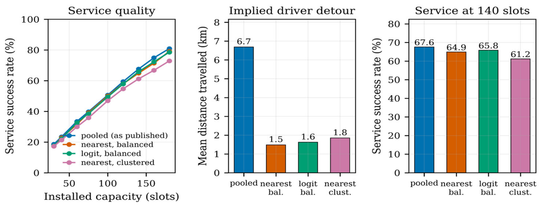
Nearest available, clustered layout	61.2	75.7	1.8	0.121

and Figure 15 report the comparison at 140 slots; the full capacity sweep is shown in the figure.

The most informative column is the distance travelled. Under the published rule the average assigned vehicle drives 6.7 km to reach its charger, because a randomly ordered station list is indifferent to location; under a nearest-available rule the same fleet drives 1.5 km. A 6.7 km detour is not plausible behaviour for workplace charging, so the aggregated rule should be read as describing a network in which drivers are perfectly flexible about where they charge. It is an optimistic bound rather than a neutral simplification, and the size of the optimism can now be stated. Introducing distance-sensitive choice on an evenly distributed network costs 2.7 percentage points of service at 140 slots, 67.6% falling to 64.9%, and about 1.8 points at 180 slots. Which behavioural rule is used matters little—nearest-available and distance-logit choice differ by about one point—because both concentrate demand on nearby stations in much the same way.

The layout matters considerably more than the choice rule. Clustering the same 35 stations into three groups reduces the service rate to 61.2% at 140 slots, 6.4 points below the aggregated figure, and to 72.9% at 180 slots, 8.1 points below. The penalty grows with capacity, and that is the substantive finding: in a small network almost every vehicle is turned away for want of a free slot anywhere, so where the slots sit hardly matters, whereas in a well-provisioned network the residual failures are increasingly vehicles that cannot reach an available charger within their acceptable detour. Beyond a moderate capacity, in other words, spatial mismatch rather than raw capacity becomes the binding constraint, and additional slots placed in the wrong districts buy progressively less service. The utilisation inequality moves in the same direction, the Gini coefficient rising from 0.103 under pooled assignment to 0.122 under the clustered layout, confirming that the imbalance the aggregated model cannot represent is real, though for a fleet whose origins are spread uniformly it remains moderate. The mean waiting time is not a useful discriminator here: it falls slightly under clustering, from 76.1 to 75.7 min, because the vehicles that do get served are disproportionately those close to a cluster and are served quickly, while distant vehicles are never served at all and enter the average at the censoring threshold. This is a selection effect and a further reason to read the waiting-time indicator as a bounded congestion index rather than as an expected delay.

Two conclusions follow for the results reported earlier. The absolute service percentages in Table 5 are upper bounds: a spatially realistic network of the same size delivers roughly one to six points less, depending on how well its stations are sited. The comparative structure of the results, however, is unaffected. The service–capacity relationship does not saturate within the tested range under any of the four assignment rules, and repeating the decision analysis of Section 5.4 on each set of spatial results returns an optimum in the same band of Scenarios 7 to 9 in every case, though not always the same member of it: Scenario 8 under pooled and distance-logit assignment, Scenario 9 under nearest-available assignment on a balanced layout, and Scenario 7 when the stations are clustered. The recommended capacity band is therefore robust to how vehicles are assigned, while the point within it is not—which is consistent with the weight-sensitivity of Section Robustness of the Ranking to Simulation and Weight Uncertainty and reinforces the reading that the band, rather than a single configuration, is what this evidence supports. The spatial layer also makes an additional planning question expressible that the pooled model could not pose at all: for a fixed number of slots, how much service is gained by siting them well. On these layouts that difference is 3.7 percentage points at 140 slots, comparable to the gain from adding roughly ten to fifteen slots, and it is available at no hardware cost.

5.8. Suitability for Practical Use and Future Work

From a sustainability standpoint the framework’s value is that it makes the resource cost of capacity explicit: charging hardware carries embodied material and manufacturing impact, so installing chargers that then sit idle is a resource cost as well as a capital one. Two quantities have to be kept apart here, and the analysis separates them. Service quality differs decisively across the configurations in the compromise band: paired over the thirty common seeds, Scenario 8 serves 7.7 percentage points more of the fleet than Scenario 7 and Scenario 9 a further 6.2 points, both far outside sampling error. What cannot be separated is the scalarised closeness coefficient under one weight vector, which is a property of the aggregation rather than of the evidence. Hardware efficiency moves in the opposite direction and does so monotonically across the whole design, from 3.13 vehicles per installed slot at 30 slots to 2.41 at 140 and 2.26 at 180. Because it always favours the smallest network, it cannot serve as a tie-breaker within the band; it is a second criterion that genuinely conflicts with service quality and with monetary cost, and the planner has to weigh it explicitly rather than read it off a single aggregate score. The same tool quantifies the alternative to building more: because the binding constraint is peak concurrency, reshaping the arrival intensity through pricing or workplace-charging incentives raises the effective service rate at fixed hardware and avoids the embodied impact of additional chargers, and the framework evaluates such demand-shifting directly by reshaping the arrival-intensity function, which is carried out quantitatively in Section 5.5.2. These levers tie the planning tool to concrete sustainability outcomes—material efficiency and deferred build-out—rather than to a generic decarbonisation claim.

On the basis of the evaluation, the system is suitable for simulating charging-station operation and analysing infrastructure behaviour, and can be used for planning station capacity, analysing demand peaks, testing new vehicle-assignment strategies, researching energy-network optimisation, and as a basis for extended smart-grid simulation. Future work could extend the system with explicit geographical modelling, dynamic electricity prices, advanced optimisation algorithms for assignment, and the integration of renewable energy sources and stationary storage, so that the planning of charging infrastructure can be coupled directly to the decarbonisation of the wider energy system.

6. Conclusions

This work designed and implemented a system for simulating EV charging that combines hierarchical Bayesian modelling with agent-based discrete-event simulation. The ACN-Data dataset was analysed and used to fit a probabilistic model capable of predicting charging behaviour—chiefly the delivered energy and the fulfilment of user requests—with partial pooling providing stable, transferable, uncertainty-aware parameter estimates. A modular simulator built on the inferred parameters reproduced vehicle arrivals, slot assignment, queue management and performance evaluation over a 24 h horizon. The energy model was validated against the data with a well-calibrated posterior-predictive check (90% coverage of 0.899). Across nine infrastructure configurations for a fixed fleet of 500 vehicles, the service success rate rose from 19% to 81% as capacity grew from 30 to 180 slots; because the long workplace dwell times limit slot turnover, full service was not reached within the tested range for that fleet, so capacity rather than daily energy is the binding constraint; a sensitivity analysis over fleet sizes from 300 to 1000 vehicles and over abandonment thresholds from one to four hours confirms that this concurrency-limited behaviour is robust, while the absolute service percentages are specific to the fleet assumed. The model was further validated out of sample on ten stations withheld from fitting, where calibration was preserved (90% interval coverage of 0.904), and benchmarked against deterministic and completely pooled alternatives: it outperforms a fixed-average rule decisively while matching, rather than exceeding, pooled regression in point accuracy, which locates its advantage in quantified uncertainty rather than in sharper prediction. A multi-criteria decision analysis (TOPSIS) over the nine scenarios placed the balanced-weighting compromise in a band of roughly 140–180 slots; a paired bootstrap over the common random numbers, which exploits the fact that every configuration is simulated with the same seeds and the same fleet, identifies that optimum sharply—the coefficient gaps are several times their bootstrap standard deviation. The uncertainty that matters is not statistical but preferential: the same configuration is optimal for only about a tenth of the weight simplex, and the recommendation moves across the band from 140 to 180 slots as the planner’s priorities shift. Two further analyses qualify the recommendation. A segmented cost model—per-station fixed costs, AC versus DC chargers, grid reinforcement scaled to the simulated peak load, and annual operating expenditure as a separate criterion—leaves the compromise plateau where the slot proxy put it. Splitting cost across two near-collinear criteria dilutes that dimension to about three-quarters of its intended weight, which is reported as a methodological caution: adding criteria that duplicate one another changes the geometry of the aggregation without adding information. Conversely, holding hardware fixed and spreading the arrival peak raises the service rate from 67% to 83%, matching what a 29% capacity expansion would deliver, so demand-side measures dominate construction once peak concurrency is the binding constraint. Monetary cost and embodied material order the candidate networks differently—hardware per unit of service delivered falls monotonically with size, while every cost specification places the optimum mid-range—and the framework reports both rather than concealing the difference in a single score. A third extension replaces the pooled vehicle-assignment rule with an explicit street grid, station coordinates, network travel distances and a preference for nearby charging. The pooled rule turns out to imply an average detour of 6.7 km, against 1.5 km when drivers choose the nearest available charger, so the service percentages reported here are upper bounds; a spatially realistic network of the same size loses about three percentage points when stations are evenly distributed and about six when the same stations are clustered, with the penalty growing as capacity rises because spatial mismatch progressively replaces raw capacity as the binding constraint. The compromise plateau and its ranking survive all four assignment rules, so the recommendation is robust to this modelling choice even though the service level attached to it is not. The principal contribution is a reproducible modelling tool that couples probabilistic modelling and multi-criteria decision making with discrete-event simulation of the charging process, providing a sound basis for capacity planning, demand-peak analysis and the design of intelligent charging strategies in support of sustainable electromobility.

The novelty of this work lies in the coupling rather than in any of its three components taken separately, each of which is established in its own literature. Hierarchical Bayesian models have been applied to charging demand, agent-based and discrete-event simulators to charging networks, and multi-criteria methods to the siting and sizing of infrastructure. What has not previously been assembled is a single pipeline in which behavioural parameters inferred with partial pooling from an open dataset drive a network simulation, whose emergent network-level indicators are then carried into an explicit and preference-transparent decision step, with the uncertainty of each stage propagated into the next and reported at the end. Three features distinguish the resulting framework from earlier work that combines Bayesian inference with simulation. First, because the behavioural model is partially pooled rather than station-specific, its parameters transfer to hypothetical networks that do not yet exist, and the out-of-sample test of Section 3.4.1 shows that this transfer preserves calibration; this is what makes the tool usable ex ante for planning rather than only ex post for analysis. Second, the decision step is not a post hoc ranking of simulation outputs but is treated as a statistical object in its own right: the Monte Carlo uncertainty of the simulator is propagated into the closeness coefficients, so the analysis states how confidently a configuration can be recommended and, in the present case, declines to name a single optimum where the evidence does not support one. Third, the chain is built end to end on an open dataset, so both the calibration and the decision recommendation can be re-examined independently. The limitations set out in Section 5.3 delimit where the framework should and should not be applied; of these, the cost proxy is relaxed in Section 5.6. and spatial aggregation in Section 5.7, while the absence of an endogenous price-response model and of station-level heterogeneity at run time remain.