Baseline-Free Flexibility Aggregation and Target Power Tracking for Source–Load Coordination of Industrial Microgrid Clusters

Abstract

Industrial microgrids are emerging as important providers of demand-side flexibility for active distribution networks. However, their participation in source–load coordination is hindered by complex production constraints, limited dispatch executability, and the widespread reliance on baseline-based demand response mechanisms. To address these challenges, this paper proposes a baseline-free source–load coordination framework for industrial microgrid clusters. A linear state–task network (LSTN) model is employed to characterize industrial production processes while preserving equipment operation, material balance, buffer storage, and production target constraints. Based on the feasible operating regions of individual microgrids, a simplified optimal adjustable load model (OALM) is developed at the aggregator level to identify and aggregate cluster-level flexibility boundaries without disclosing detailed production information. Building upon the aggregated flexibility region, a baseline-free target power tracking strategy is established, in which the distribution network issues absolute power targets and the aggregator coordinates multiple industrial microgrids to achieve their realization. The proposed framework simultaneously ensures production feasibility, scalable flexibility aggregation, and practical dispatch implementation. Case studies demonstrate that the aggregated industrial load can accurately track dispatch targets while satisfying all production constraints, thereby enhancing the capability of industrial microgrid clusters to participate in large-scale source–load interaction and renewable energy accommodation. Case study results show that when the number of industrial microgrids increases from 10 to 200, the total computation time increases from 5.08 s to 337.40 s, while the target tracking error remains within numerical tolerance. Compared with the conventional baseline-based virtual-battery (VB) method, whose root mean square error (RMSE) with respect to the intended absolute target reaches 241.30 kW under a ±10% baseline estimation error, the proposed method achieves near-zero tracking error. In addition, the production-agnostic aggregation model expands the flexibility boundary by 21.84% and generates targets that are not exactly executable under the full LSTN production constraints.

1. Introduction

The ongoing transition toward carbon-neutral power systems has accelerated the integration of renewable energy resources into distribution networks [1]. Driven by the increasing penetration of wind and photovoltaic generation, traditional passive distribution networks are evolving into active distribution systems characterized by extensive interactions among generation, network, load, and storage resources [2]. While renewable energy integration contributes to decarbonization objectives, its intermittency and variability introduce operational challenges to distribution networks, including power fluctuations, voltage violations, congestion, and renewable energy curtailment [3,4]. These challenges motivate distribution network operators to activate demand-side flexibility. It should be clarified that voltage violations and network congestion are considered in this paper only as system-level motivations for flexibility activation. The present study does not directly formulate a distribution-network voltage-control or power-flow optimization model. Instead, it assumes that the network-side regulation direction and operating requirement have been determined through external operational analysis and focuses on the production-executable flexibility aggregation and absolute target power tracking of industrial microgrid clusters under LSTN production constraints, PV generation constraints, and PCC exchange-power limits.

Among various demand-side resources, industrial microgrids represent a particularly valuable source of flexibility [5]. Compared with residential and commercial consumers, industrial users exhibit large electricity consumption, predictable operational patterns, and substantial regulation potential. Equipped with distributed generation, local energy management systems, and controllable production processes, industrial microgrids are increasingly regarded as important participants in source–load interaction and demand-side flexibility services. Recent studies have further highlighted the evolution of microgrids from local backup power systems to active operational units capable of supporting system flexibility, resilience, and renewable energy accommodation [6].

Despite their considerable flexibility potential, industrial microgrids differ fundamentally from conventional controllable loads. The operational flexibility of industrial production processes is constrained by material conservation, process sequencing, equipment operating conditions, intermediate inventory limitations, and production completion requirements [7]. Therefore, the adjustable capacity of industrial loads cannot be adequately represented by simple upward/downward power regulation limits. Dispatch decisions that are feasible from a power-system perspective may violate production constraints and become inapplicable in industrial practice [8]. Accurate characterization of industrial production flexibility is therefore essential for enabling large-scale participation of industrial users in power system operation.

Price-based demand response has been widely used to coordinate flexible resources in microgrids. For example, Wu et al. [9] developed a demand response model considering seasonal electricity prices for islanded microgrid operation. Such studies demonstrate the value of demand-side flexibility for balancing renewable generation and electricity consumption; however, generic demand response models do not explicitly describe the task execution, material balance, and inventory constraints of industrial production processes.

To address the industrial-specific modeling challenge, considerable efforts have been devoted to production-process-oriented load modeling and flexibility evaluation. Existing reviews have systematically summarized the sources, implementation methods, and operational constraints of industrial demand response [10,11]. In particular, the linear state–task network (LSTN) represents production tasks, material flows, inventory states, and intertemporal process coupling using a tractable linear formulation [12]. Hybrid data-driven and physics-based methods have also been developed to evaluate aggregated industrial flexibility while reducing the disclosure of detailed production information [13]. More recently, Su et al. proposed the Optimal Adjustable Load Model (OALM), which projects the high-dimensional production-feasible region onto a compact power–energy representation for upper-level scheduling [14].

For scalable resource coordination, virtual-battery and aggregate feasible-region models have been extensively investigated. Tan et al. developed an optimal virtual-battery model that incorporates network constraints when aggregating storage-like resources [15], while Jangid et al. established an aggregation–scheduling–disaggregation framework for flexible loads in distribution-system operation [16]. Recent studies have further examined the disaggregation of aggregate commands among heterogeneous resources [17], coordinated aggregation between virtual power plants and distribution network operators [18], and network-aware aggregation of distributed energy resources [19]. A state-driven aggregation and scheduling method has also been developed for heterogeneous power-to-heat loads participating in market bidding [20]. Nevertheless, these models are mainly designed for generic flexible or storage-like resources and do not explicitly preserve the task execution, material balance, inventory capacity, and terminal production requirements of industrial processes. In addition, the original OALM focuses on the feasible region of an individual industrial production process, while cluster-level aggregation and executable target decomposition among multiple heterogeneous industrial microgrids remain insufficiently addressed.

Another limitation arises from the reliance of conventional demand response on estimated baseline consumption. A demand response baseline represents the counterfactual electricity consumption that would have occurred without a response event and therefore cannot be directly observed. Existing baseline-estimation methods involve trade-offs among estimation accuracy, data requirements, and implementation complexity [21]. Moreover, baseline estimation may be affected by forecasting errors and strategic manipulation by participating users [22]. Consequently, a regulation quantity defined only as a deviation from an estimated baseline may not accurately represent the absolute power that can be delivered to the distribution network.

Data-driven prediction and uncertainty-aware optimization provide complementary approaches for improving practical operation. Recent studies have investigated temporal fault prediction for industrial equipment [23], forecasting and optimal load allocation in combined heat and power systems [24], risk-aware optimization under renewable and operational uncertainties [25], and resilient control under communication attacks [26]. These studies improve prediction, risk management, and operational resilience, but they do not establish a cluster-level absolute power–energy boundary that simultaneously preserves industrial production feasibility and supports baseline-free target tracking.

The above review reveals three research gaps. First, existing industrial flexibility models do not simultaneously provide detailed production-process representation and scalable flexibility aggregation for multiple industrial microgrids [12,13,14]. Second, conventional virtual-battery and feasible-region approaches do not explicitly preserve all intertemporal production constraints when aggregate targets are decomposed among heterogeneous industrial users [15,16,17,18,19,20]. Third, baseline-based demand response may propagate baseline-estimation errors into regulation quantities and is therefore not fully suited to direct absolute-power tracking [21,22]. These gaps motivate the proposed framework, which maps local LSTN production-feasible sets into cluster-level absolute power and cumulative-energy boundaries and further decomposes the baseline-free target into executable production schedules.

Existing demand response and flexibility aggregation methods provide an important basis for industrial loads to participate in distribution network operation, but several limitations remain in the context of industrial microgrid clusters. Conventional baseline-based demand response and virtual-battery models usually use an estimated baseline as the reference and represent flexibility as a power deviation from this baseline. Therefore, their regulation performance is sensitive to baseline estimation errors. Existing baseline-free demand response methods reduce the dependence on counterfactual baselines, but most of them mainly focus on load-side target tracking or market settlement mechanisms, while the executability of industrial production processes is not fully considered. LSTN-based methods can represent the coupling among production tasks, material states, and inventory constraints, but they mainly focus on feasible scheduling of individual industrial processes rather than cluster-level flexibility boundary identification for industrial microgrids. OALM and virtual-battery-based aggregation methods can compactly describe the power and energy flexibility of load groups; however, if production-process constraints are not embedded, the obtained aggregate boundary may overestimate the actually executable flexibility.

To further clarify the difference between the proposed method and existing studies,

Table 1. Comparison between the proposed method and existing demand response and flexibility aggregation methods.

Method Category	Baseline-Free Target Power Tracking	Production-Process Executability	Cluster-Level Flexibility Boundary for Industrial Microgrids
Conventional baseline-based demand response and virtual-battery methods [15,21,22]	Usually baseline-dependent	Usually not explicitly considered	Aggregation is possible, but the boundary is affected by baseline and modeling assumptions
Existing baseline-free or direct-capacity-based coordination methods [27,28]	Can avoid baseline estimation	Industrial production processes are usually not modeled	Cluster-level boundaries for industrial microgrids are rarely provided
LSTN-based industrial-load modeling methods [12]	Can support feasible production scheduling	Production-process executability can be preserved	Cluster-level aggregate flexibility boundaries are usually not provided
Original OALM-based feasible-region modeling method [14]	Can describe adjustable-load boundaries	Depends on the embedded underlying constraints	Parameter identification is complex and difficult to extend to long-horizon cluster scenarios
Proposed method (this work)	Directly tracks absolute target power without baseline estimation	Preserves production-process executability through LSTN constraints	Identifies cluster-level flexibility boundaries considering PV and PCC constraints through a simplified OALM

compares different methods from three perspectives.

To bridge these gaps, this paper investigates a baseline-free coordinated dispatch framework for industrial microgrid clusters participating in source–load interaction with distribution networks. The proposed framework employs the linear state–task network (LSTN) model to represent industrial production processes while preserving material balance, equipment operation, and production target constraints. Based on the local feasible regions derived from the LSTN models, a time-varying OALM is developed to characterize the aggregated flexibility boundaries of the industrial microgrid cluster. Within the identified flexibility region, a baseline-free absolute power target tracking strategy is further established, enabling the cluster to directly track dispatch targets issued by the distribution network using actual aggregated power rather than baseline-referenced response quantities. To establish an explicit connection between industrial flexibility aggregation and distribution-network operation, a linearized radial power-flow model is incorporated into the proposed framework. In addition to local PCC exchange-power limits, the cluster-level flexibility boundaries and the final dispatch trajectory are constrained by nodal power balance, bus-voltage limits, and branch thermal capacities. Therefore, the flexibility reported to the DNO represents the deliverable flexibility that can be accommodated by the feeder without causing voltage violations or branch congestion. The main contributions of this work are summarized as follows:

(1)

A baseline-free source–load coordination framework is proposed for industrial microgrid clusters. Different from conventional baseline-based demand response and virtual-battery methods, the proposed framework does not use an estimated baseline as the regulation reference. Instead, it directly generates and tracks the target power trajectory in the absolute power space of the industrial microgrid cluster, thereby avoiding the propagation of baseline estimation errors into dispatch results.

(2)

An industrial microgrid load aggregation method that preserves production-process executability is developed. The LSTN production-process constraints are embedded into the industrial microgrid operation and aggregation dispatch model, so that the obtained regulation trajectory satisfies not only power and energy constraints but also task execution, material balance, inventory capacity, and terminal production requirements.

(3)

A simplified OALM-based flexibility boundary identification method is constructed for industrial microgrid clusters. Compared with the original OALM and conventional virtual-battery-based aggregation methods, the proposed method incorporates PV generation constraints, local PCC exchange-power limits, bus-voltage limits, and branch thermal-capacity constraints into cluster-level flexibility boundary identification while preserving production executability. It thereby provides an explicit and network-feasible power–energy boundary for target power generation at the distribution-network level.

The effectiveness of the proposed framework is validated through comprehensive case studies involving industrial microgrid clusters under various operating conditions, demonstrating its capability to accurately identify aggregated flexibility boundaries and achieve reliable target power tracking while maintaining industrial production feasibility.

2. System Framework and Industrial Microgrid Modeling

2.1. Baseline-Free Source–Load Coordination Framework

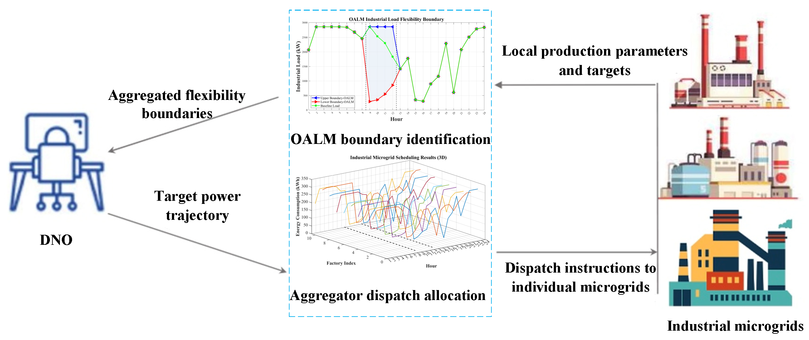
The proposed source–load coordination framework consists of a distribution network operator (DNO), an aggregator, and multiple industrial microgrids (IMGs), as illustrated in Figure 1. The DNO determines the desired power regulation trajectory according to system operational requirements, while the aggregator serves as an intermediary between the distribution network and industrial users.

The coordination process is implemented in two stages. First, each industrial microgrid reports its operational flexibility to the aggregator based on local production conditions, equipment status, and renewable generation forecasts. The aggregator then derives the aggregated flexibility region of the industrial microgrid cluster and communicates it to the DNO. Second, the DNO issues a target power trajectory within the reported flexibility boundaries. The aggregator subsequently allocates the regulation task among individual industrial microgrids while ensuring the feasibility of local production processes.

Unlike conventional demand response schemes that quantify flexibility relative to an estimated baseline load, the proposed framework adopts a baseline-free dispatch paradigm. The performance of the industrial microgrid cluster is evaluated directly according to the deviation between the actual aggregated power and the target power specified by the DNO. This formulation eliminates the dependence on baseline estimation and improves the transparency and executability of dispatch decisions.

Each industrial microgrid consists of distributed photovoltaic (PV) generation, industrial production loads, auxiliary loads, and a point of common coupling (PCC) connected to the distribution network. Since industrial production loads constitute the primary source of operational flexibility, an accurate representation of production-process constraints is essential. Therefore, this paper employs the LSTN model to characterize industrial production systems.

The LSTN model adopted in this paper is based on the following assumptions. First, the scheduling horizon is divided into discrete time intervals, and the processing time of industrial production tasks can be continuously allocated within these intervals. Second, material consumption, material generation, and power consumption during task execution are represented by linear coefficients, meaning that a fixed amount of material conversion and power consumption is associated with a unit processing time. Under these assumptions, the proposed framework is applicable to industrial processes with clear production routes, relatively stable material conversion relationships, and electricity consumption characteristics that can be reasonably approximated by linear models.

For industrial processes with weak to moderate nonlinearities, piecewise linearization or local linear approximation can be incorporated into the proposed framework. For example, energy consumption coefficients or production coefficients under different operating regions can be represented using piecewise linear parameters. For processes with strongly nonlinear dynamics, complex equipment state transitions, or significant stochastic behavior, the current linear LSTN model may not fully capture the underlying dynamics and should be extended to mixed-integer nonlinear models, scenario-based stochastic optimization models, or data-driven approximations. Operating uncertainties such as PV forecast errors, production disturbances, and equipment failures can be addressed in future work by combining rolling optimization, real-time OALM boundary updating, and reserve-margin allocation. When unexpected disturbances significantly change the production feasible region, the flexibility boundary needs to be re-identified and the dispatch strategy needs to be regenerated.

2.2. LSTN-Based Industrial Process Model

Industrial load flexibility originates from the adjustable operation of production processes. To preserve production feasibility during dispatch, the industrial process is represented using LSTN, in which production activities are modeled as tasks and material inventories are represented as states.

(1)

Task Scheduling Model

Consider an industrial process comprising a set of production tasks $I=\left\{1,2,\dots ,i^{\mathrm{end}}\right\}$. Each task $i\in I$ may operate at multiple operating points $K_i$ associated with different power consumption levels and production rates. Associated with each task are “states,” including raw materials, intermediate products, and final products, denoted as the set s = {0} ∪ I, where s = 0 represents the raw material state and s = i represents the intermediate product state produced by task $i$. The inventory of state at time t is denoted as $S_{s,t}$, which changes dynamically under the influence of task operations.

(2)

Power Consumption and Time Resource Constraints

Let the power consumption of task $i$ at operating point k be $P_{i,k}$, and let the duration for which it operates at this point within dispatch period $t$ be $\Delta t_{i,k,t}$. Then, the total power consumption of the factory $P_t^{\mathrm{fact}}$ can be expressed as the time-weighted sum of the power at each operating point across all tasks:

$$P_t^{\mathrm{fact}}={\displaystyle \sum _{i\in I}{\displaystyle \sum _{k\in K_i}{P}_{i,k}}}\cdot {\displaystyle \frac{\Delta t_{i,k,t}}{\Delta T}}$$

(1)

where $\Delta T$ is the dispatch step size, and T is the set of dispatch periods.

For each task, the sum of operating durations across all operating points within any dispatch period must equal the dispatch step size, and each operating duration must be non-negative:

$${\displaystyle \sum _{k\in K_i}\Delta t_{i,k,t}}=\Delta T,\hspace{1em}\forall i\in I,t\in T$$

(2)

$$\Delta t_{i,k,t}\ge 0,\hspace{1em}\forall i\in I, k\in K, t\in T$$

(3)

Equation (2) ensures that the time allocation of a task across its operating points fully covers the entire dispatch period, allowing the equipment to switch operating points within a period. Equation (3) guarantees the physical validity of the time variables.

(3)

Production Process Constraints

The material flow in the production process is driven by task operations. Each task i at operating point k produces material at a rate $G_{i.k}$ (kg/h) and consumes material at a rate $C_{i,k}$. For the raw material state $s=0$, its inventory change is affected only by consumption:

$$S_{0,t}=S_{0,t-1}-{\displaystyle \sum _{k\in K_1}{C}_{1,k}}\Delta t_{1,k,t},\hspace{1em}\forall t\in T$$

(4)

For an intermediate product state $s=i,\hspace{0.33em}\hspace{0.33em}i\in I\backslash \left\{i^{\mathrm{end}}\right\}$, its inventory is simultaneously affected by the production of task $i$ and the consumption of the subsequent task $i+1$:

$$S_{i,t}=S_{i,t-1}+{\displaystyle \sum _{k\in K_i}{G}_{i,k}}\Delta t_{i,k,t}-{\displaystyle \sum _{k^{\prime }\in K_{i+1}}{C}_{i+1,k^{\prime }}}\Delta t_{i+1,k^{\prime },t},\forall t\in T,i\in I\backslash \{i^{end}\}$$

(5)

For the final product state $s=i^{\mathrm{end}}$, its inventory is affected only by the production of task $i^{\mathrm{end}}$ with no subsequent consumption; thus, only the production term is retained in a form analogous to Equation (5):

$$S_{i^{\mathrm{end}},t}=S_{i^{\mathrm{end}},t-1}+{\displaystyle \sum _{k\in K_{\mathrm{end}}}{G}_{i^{\mathrm{end}},k}}\Delta t_{i^{\mathrm{end}},k,t}$$

(6)

Equations (4)–(6) describe the material-inventory evolution under the assumptions adopted in this study. Specifically, the model considers a finite scheduling horizon and a serial production process. The raw materials required during the scheduling horizon are assumed to be available in the initial inventory, with no external replenishment during the horizon. Final products are retained within the production system during the scheduling horizon and are shipped after the horizon. Therefore, the raw-material state contains only consumption terms, whereas the final-product state contains only production terms. All material inventories remain subject to the non-negativity and storage-capacity constraints given below. The $i+1$ notation denotes the subsequent task in the serial production process considered in this study. Processes involving within-horizon material deliveries, product shipments, or branching and converging production flows are outside the scope of the current model and can be addressed by introducing external inflow/outflow terms and a general state–task incidence representation.

(4)

Material Conservation and Buffer Dynamics

Equations (4)–(6) describe the dynamic evolution of material inventories, while Equations (7)–(9) specify the boundary conditions and production target constraints. The physical meaning of each equation is elaborated below.

(1) Initial condition constraint

$$S_{s,0}=S_s^{\mathrm{initial}},\hspace{1em}\forall s\in S$$

(7)

At the start of the dispatch horizon ($t=0$), the inventory of each state is known.

(2) Upper and lower bound constraints

$$0\le S_{s,t}\le S_s^{\max },\hspace{1em}\forall s\in S,\hspace{1em}t\in T$$

(8)

The inventory of each material must remain within safe limits at all times. The lower bound of zero ensures no negative inventory, while the upper bound $S_s^{\max }$ is determined by the physical storage capacity.

(3) Production target constraint

$$S_{s,t}\ge S_s^{\mathrm{target}}+S_s^{\mathrm{initial}}, t=t^{\mathrm{end}}, s\in S$$

(9)

At the end of the dispatch horizon, the inventory of each state must not fall below the sum of its initial inventory and the target net production. Equation (9) uses an inequality rather than an equality, providing flexibility in dispatch optimization—allowing the final inventory to exceed the target value, but not to fall below it.

(5)

Photovoltaic Output Modeling

Let $P_t^{\mathrm{PV}}$ be the actual output of the PV array within the microgrid during period t, and let $P_t^{\mathrm{PV},\mathrm{forecast}}$ be the forecasted upper bound of PV generation. The PV output is then subject to the following constraint:

$$0\le P_t^{\mathrm{PV}}\le P_t^{\mathrm{PV},\mathrm{forecast}},\hspace{1em}\forall t\in T$$

(10)

This paper assumes that the PV forecast is known and focuses on the optimal dispatch strategy of the microgrid under given PV output scenarios.

The PV generation forecast is treated as a given input in the current dispatch model. Therefore, the proposed framework is formulated as a deterministic optimization model rather than a stochastic scenario-based optimization model.

2.3. Industrial Microgrid Operational Model

(1)

Power Balance Constraint

The industrial microgrid exchanges power with the upstream distribution network through the PCC. Assuming lossless operation within the microgrid, the power balance relationship is expressed as:

$$P_t^{\mathrm{PCC}}=P_t^{\mathrm{fact}}-P_t^{\mathrm{PV}},\hspace{1em}\forall t\in T$$

(11)

where $P_t^{\mathrm{PCC}}$ denotes the net power exchanged between the industrial microgrid and the distribution network during dispatch interval (t). Positive values indicate electricity import from the grid, whereas negative values represent electricity export.

(2)

Objective Function

The operational objective of the industrial microgrid is to minimize the total electricity transaction cost over the scheduling horizon. Let ${\lambda }_t$ denote the time-varying electricity price during period t. Assuming identical buying and selling prices, the operating cost is formulated as:

$$\min Cost={\displaystyle \sum _{t\in T}{\lambda }_t}\cdot (P_t^{\mathrm{fact}}-P_t^{\mathrm{PV}})\cdot \Delta t$$

(12)

The optimization problem defined by (1)–(12) determines the economically optimal operation of the industrial microgrid while satisfying production-process constraints, material balance requirements, and renewable generation limits. The resulting feasible operating region serves as the foundation for the flexibility aggregation and coordinated dispatch models developed in the subsequent sections.

3. Aggregated Flexibility Characterization and Coordinated Dispatch of Industrial Microgrid Clusters

Building upon the industrial microgrid model developed in Section 2, this section investigates the coordinated participation of multiple industrial microgrids in distribution-network demand response. A hierarchical coordination framework consisting of the DNO, an aggregator, and industrial microgrids is established. To preserve the privacy of individual production processes while enabling system-level optimization, the adjustable capability of industrial microgrids is represented through the OALM, which provides a compact characterization of cluster-level flexibility.

3.1. OALM-Based Aggregated Flexibility Boundary Identification

In the construction of the cluster-level OALM, the feasible region of each industrial microgrid is first determined by its production-process constraints and operational constraints. For the $m$-th industrial microgrid, the feasible region is jointly defined by the LSTN production-process constraints, PV generation constraints, and PCC exchange-power constraints, and can be expressed as ${\Omega }_m=\left\{x_m\right| {\mathcal{C}}_m^{\mathrm{LSTN}},{\mathcal{C}}_m^{\mathrm{PV}},{\mathcal{C}}_m^{\mathrm{PCC}}\}$, where ${\mathcal{C}}_m^{\mathrm{LSTN}}$ denotes the production-process constraints, including task execution, material balance, inventory capacity, and terminal production requirements; ${\mathcal{C}}_m^{\mathrm{PV}}$ denotes the PV generation constraints; and ${\mathcal{C}}_m^{\mathrm{PCC}}$ denotes the upper and lower limits of PCC exchange power. The feasible region of the industrial microgrid cluster is expressed as the Cartesian product of individual feasible regions: $\Omega ={\Omega }_1\times {\Omega }_2\times \dots \times {\Omega }_M$.

Based on this feasible region, the lower and upper aggregate power boundaries at time period $t$ are identified by solving the following optimization problems: ${\underset{\_}{P}}_t={\min }_{x\in \Omega }{\displaystyle \sum _{m=1}^M{P}_{m,t}}$ and ${\overline{P}}_t={\max }_{x\in \Omega }{\displaystyle \sum _{m=1}^M{P}_{m,t}}$, where $P_{m,t}$ is the actual power consumption of the $m$-th industrial microgrid at time period $t$. Since the material balance, inventory states, and terminal production requirements in the LSTN constraints introduce inter-temporal coupling, a sequential time-period identification procedure is adopted for power boundary construction. Specifically, when identifying the power boundary at time period $t$, the previously identified boundary values are fixed as ${\displaystyle \sum _{m=1}^M{P}_{m,\tau }}={\underset{\_}{P}}_{\tau },\hspace{1em}\tau =1,\dots ,t-1$ for lower-boundary identification, or ${\displaystyle \sum _{m=1}^M{P}_{m,\tau }}={\overline{P}}_{\tau },\hspace{1em}\tau =1,\dots ,t-1$ for upper-boundary identification. In this way, the obtained boundary trajectory reflects the hourly power regulation capability while preserving the impact of inter-temporal production coupling on subsequent feasibility.

The cumulative energy boundaries describe the adjustable range of the total cluster electricity consumption over the scheduling horizon and are obtained by $\underset{\_}{E}={\min }_{x\in \Omega }{\displaystyle \sum _{t\in T}{\displaystyle \sum _{m=1}^M{P}_{m,t}}}\Delta t$, $\overline{E}={\max }_{x\in \Omega }{\displaystyle \sum _{t\in T}{\displaystyle \sum _{m=1}^M{P}_{m,t}}}\Delta t$. Thus, the cluster-level OALM is represented by the combination of the power boundaries ${\{{\underset{\_}{P}}_t,{\overline{P}}_t\}}_{t\in T}$ and the cumulative energy boundary $[\underset{\_}{E},\overline{E}]$, which provides a feasibility reference for DNO target power generation and aggregator dispatch.

The flexibility available from an industrial microgrid cluster originates from the adjustable operation of industrial production processes. To characterize this flexibility at the aggregation level, this paper adopts the OALM. Unlike conventional virtual-battery models that describe flexibility through baseline-referenced charging/discharging power and cumulative regulation energy, OALM directly models the aggregated industrial production load and derives its feasible power and energy boundaries over the demand response horizon. Consequently, the identified flexibility region is independent of baseline estimation and can be directly utilized for dispatch decision-making.

Let F denote the set of industrial microgrids and T_DR the demand response horizon. The aggregated industrial production load $P_t^{\mathrm{agg}}$ is expressed as:

$$P_t^{\mathrm{agg}}={\displaystyle \sum _{f\in F}{P}_{f,t}^{\mathrm{load}}}$$

(13)

where $P_{f,t}^{\mathrm{load}}$ denotes the industrial production load of microgrid f during period t, which is determined by the LSTN-based production process model described in Section 2.

Based on (13), the OALM identifies four flexibility parameters, namely the lower and upper power boundaries and the lower and upper cumulative energy boundaries. The corresponding optimization model is formulated as

$$\max \hspace{1em}{\eta }^{\mathrm{T}}\left[{\underset{\_}{P}}_t^{\mathrm{O}};{\overline{P}}_t^{\mathrm{O}};{\underset{\_}{E}}^{\mathrm{O}};{\overline{E}}^{\mathrm{O}}\right]$$

(14)

$$\mathrm{s}.\mathrm{t}. \hspace{1em}{\underset{\_}{P}}_t^{\mathrm{O}}\le P_t^{\mathrm{agg}}\le {\overline{P}}_t^{\mathrm{O}},\hspace{1em}t\in T_{\mathrm{DR}}$$

(15)

$${\underset{\_}{E}}^{\mathrm{O}}\le {\displaystyle \sum _{t\in T_{\mathrm{DR}}}{P}_t^{\mathrm{agg}}}\Delta t\le {\overline{E}}^{\mathrm{O}}$$

(16)

$$-{\overline{P}}^{\mathrm{O}}\Delta t+{\overline{E}}^{\mathrm{O}}\le 0$$

(17)

$$-{\underset{\_}{P}}^{\mathrm{O}}\Delta t+{\underset{\_}{E}}^{\mathrm{O}}\ge 0$$

(18)

$$\left(1\right)\sim \left(11\right), f\in F$$

(19)

where $\eta$ is a vector of weight coefficients used to identify the lower power boundary, upper power boundary, lower energy boundary, and upper energy boundary in the OALM; ${\underset{\_}{P}}_t^{\mathrm{O}}$ and ${\overline{P}}_t^{\mathrm{O}}$ denote the scalar forms of the lower and upper aggregated power boundaries during the demand response periods. Equation (19) indicates that the four parameters of the model are also subject to the LSTN model constraints and must not violate the factory modeling requirements.

3.2. Distribution Network Target Power Optimization

After obtaining the aggregated flexibility boundaries, the DNO determines a target power trajectory within the feasible flexibility region. In this paper, “baseline-free” refers specifically to the absence of a counterfactual no-response load baseline in flexibility characterization and coordinated dispatch. Conventional baseline-based demand response requires estimating the load that would have occurred without a response event. Such a baseline cannot be directly observed during the event, and its estimation errors or strategic manipulation may affect the quantified response [22,29,30]. In contrast, no estimated baseline is used as a variable, parameter, or reference trajectory in the proposed OALM boundary-identification, DNO target-generation, or aggregator dispatch models.

The proposed framework does not address incentive payment or market settlement; therefore, “baseline-free” does not imply that all possible incentive mechanisms are necessarily independent of baselines. The tracking-error penalty used in the dispatch objective is a numerical optimization coefficient rather than an incentive payment.

The DNO first determines the response period and regulation direction according to an external system operating requirement. It then generates the target trajectory directly within the absolute lower/upper power and cumulative-energy boundaries reported by the aggregator. The trajectory-smoothing term restricts changes between consecutive target values and does not introduce a counterfactual load reference. Accordingly, the target is an absolute power command rather than a baseline-relative regulation quantity. This absolute-power representation is consistent with recent capacity-limitation and desired-load-profile approaches that define demand-side flexibility using directly specified power limits or target trajectories [27,28]. Conventional operating load curves presented in the case studies are used only for visualization and comparative evaluation and do not enter the proposed optimization models.

Let $P_t^{\mathrm{tar}}$ denote the target industrial load during period t. To ensure dispatch feasibility, the target trajectory must satisfy the OALM-derived power and energy constraints. In addition, excessive fluctuations between consecutive dispatch intervals are undesirable from both operational and control perspectives. Therefore, a trajectory smoothness constraint is incorporated into the optimization model. The DNO target generation model is formulated as

$$\min \hspace{1em}{\omega }_P{\displaystyle \sum _{t\in T_{\mathrm{DR}}}{P}_t^{\mathrm{tar}}}\Delta t+\rho {\displaystyle \sum _{t\in T_{\mathrm{DR}}\setminus \left\{t_0\right\}}{\left(P_t^{\mathrm{tar}}-P_{t-1}^{\mathrm{tar}}\right)}^2}$$

(20)

$$\mathrm{s}.\mathrm{t}.\hspace{1em}{\underset{\_}{P}}^{\mathrm{O}}\le P_t^{\mathrm{tar}}\le {\overline{P}}^{\mathrm{O}},\hspace{1em}t\in T_{\mathrm{DR}}$$

(21)

$${\underset{\_}{E}}^{\mathrm{O}}\le {\displaystyle \sum _{t\in T_{\mathrm{DR}}}{P}_t^{\mathrm{tar}}}\Delta t\le {\overline{E}}^{\mathrm{O}}$$

(22)

$$-R^{\max }\le P_t^{\mathrm{tar}}-P_{t-1}^{\mathrm{tar}}\le R^{\max },\hspace{1em}t\in T_{\mathrm{DR}}\setminus \left\{t_0\right\}$$

(23)

where $\rho$ is the weight for target trajectory smoothness, $R^{\max }$ is the maximum allowable change in target power between adjacent periods, and $t_0$ is the start period of the demand response horizon. The parameter ${\omega }_P$ is used to unify the distribution network objectives under different regulation directions. When ${\omega }_P=1$, the model minimizes the total industrial load energy during the demand response periods, corresponding to peak shaving or load reduction. When ${\omega }_P=-1$, the model equivalently maximizes the total industrial load energy during the demand response periods, corresponding to valley filling, load increase, or renewable energy accommodation.

The resulting target trajectory always remains within the aggregated flexibility boundaries identified by OALM and satisfies both cumulative energy and ramping constraints. Consequently, it provides a physically realizable dispatch target for subsequent coordination by the aggregator.

3.3. Aggregator Dispatch Allocation Model

During cluster-level flexibility boundary identification, the LSTN production constraints, PV availability constraint, microgrid power-balance equation, and PCC exchange-power limits of each industrial microgrid are incorporated into the same detailed feasible set. First, the LSTN determines the industrial production load according to the production tasks, material balances, inventory capacities, and terminal production requirements. The PV output is then constrained by its available generation, and the PCC exchange power is calculated through the microgrid power-balance equation. Finally, the lower and upper PCC exchange-power limits are imposed. The cluster industrial load is obtained by summing the industrial production loads of all microgrids, and both the power and cumulative-energy boundaries are identified over this complete feasible set. Consequently, PV availability and PCC capacity directly affect the identified cluster-level flexibility boundaries, and each identified extreme-boundary trajectory is supported by a dispatch schedule satisfying the complete production and microgrid operating constraints. The distribution-network-related constraints considered in the current model mainly include microgrid power balance and PCC exchange-power limits; bus-voltage, branch-power-flow, and network-topology constraints are outside the scope of the present study.

Given the target trajectory $P_t^{\mathrm{tar}}$ issued by the DNO, the aggregator allocates regulation tasks among individual industrial microgrids while coordinating industrial production loads, photovoltaic generation, and power exchanges with the distribution network.

Let $P_{f,t}^{\mathrm{load}}$, $P_{f,t}^{\mathrm{pv}}$, and $P_{f,t}^{\mathrm{pcc}}$ denote the industrial production load, photovoltaic output, and PCC power exchange of microgrid f, respectively. The aggregator determines the optimal dispatch strategy by minimizing the total operating cost while tracking the target aggregated industrial load. The optimization problem is formulated as:

$$\min \hspace{1em}{\displaystyle \sum _{f\in F}{\displaystyle \sum _{t\in T}{\lambda }_t}}{P}_{f,t}^{\mathrm{pcc}}\Delta t+M{\displaystyle \sum _{t\in T_{\mathrm{DR}}}\left(\Delta P_t^{+}+\Delta P_t^{-}\right)}$$

(24)

$$\mathrm{s}.\mathrm{t}.\hspace{1em}{\displaystyle \sum _{f\in F}{P}_{f,t}^{\mathrm{load}}}-P_t^{\mathrm{tar}}=\Delta P_t^{+}-\Delta P_t^{-},\hspace{1em}t\in T_{\mathrm{DR}}$$

(25)

$$\Delta P_t^{+}\ge 0,\hspace{1em}\Delta P_t^{-}\ge 0,\hspace{1em}t\in T_{\mathrm{DR}}$$

(26)

$$P_{f,t}^{\mathrm{pcc}}=P_{f,t}^{\mathrm{load}}-P_{f,t}^{\mathrm{pv}},\hspace{1em}f\in F,\hspace{0.33em}t\in T$$

(27)

$$0\le P_{f,t}^{\mathrm{pv}}\le P_{f,t}^{\mathrm{pv},\mathrm{av}},\hspace{1em}f\in F,\hspace{0.33em}t\in T$$

(28)

$$P_f^{\mathrm{pcc},\min }\le P_{f,t}^{\mathrm{pcc}}\le P_f^{\mathrm{pcc},\max },\hspace{1em}f\in F,\hspace{0.33em}t\in T$$

(29)

$$\left(1\right)\sim \left(12\right),\hspace{1em}f\in F,\hspace{0.33em}t\in T$$

(30)

where ${\lambda }_t$ is the electricity purchase price during period t; M is the penalty coefficient for target power tracking error; and $\Delta P_t^{+}$ and $\Delta P_t^{-}$ denote the positive and negative deviations of the aggregated industrial load from the distribution network target power, respectively.

The objective function consists of two components: the electricity transaction cost associated with PCC power exchange and a penalty term reflecting deviations from the target trajectory. The tracking requirement is imposed on the aggregated industrial production load. By integrating the flexibility characterization model, the DNO target generation model, and the aggregator allocation model, a complete baseline-free coordinated dispatch framework is established. The proposed framework enables industrial microgrid clusters to provide verifiable and production-feasible flexibility services to the distribution network while maintaining the privacy of individual industrial processes.

Based on the above aggregator dispatch model, the achievable lower and upper limit trajectories and the corresponding target-violation handling mechanism are defined as follows.

Let $\mathcal{X}$ denote the detailed cluster feasible set containing all LSTN production constraints, PV availability constraints, microgrid power-balance equations, and PCC exchange-power limits, and let $P_t^{\mathrm{agg}}(x)$ denote the aggregate industrial load associated with dispatch schedule $x\in \mathcal{X}$. The OALM-identified lower boundary ${\underset{\_}{P}}_t^{\mathrm{OALM}}$ and upper boundary ${\overline{P}}_t^{\mathrm{OALM}}$ are separately used as the targets of the aggregator dispatch model. For $s\in \{-,+\}$, let $B_t^{-}={\underset{\_}{P}}_t^{\mathrm{OALM}}$ and $B_t^{+}={\overline{P}}_t^{\mathrm{OALM}}$. The corresponding dispatch schedule is defined as

$$x^{\mathrm{ach},s}\in \arg {\min }_{x\in \mathcal{X}}\left[M{\displaystyle \sum _{t\in {\mathcal{T}}_{\mathrm{DR}}}\left|P_t^{\mathrm{agg}}(x)-B_t^s\right|}+C^{\mathrm{elec}}(x)\right]$$

(31)

where $M$ is the tracking-deviation penalty coefficient and $C^{\mathrm{elec}}(x)$ is the electricity transaction cost. The achievable lower and upper limit trajectories are respectively defined as ${\underset{\_}{P}}_t^{\mathrm{ach}}=P_t^{\mathrm{agg}}\left(x^{\mathrm{ach},-}\right)$, ${\overline{P}}_t^{\mathrm{ach}}=P_t^{\mathrm{agg}}\left(x^{\mathrm{ach},+}\right)$. Because $x^{\mathrm{ach},-}$ and $x^{\mathrm{ach},+}$ both belong to $\mathcal{X}$, the two achievable limit trajectories are supported by dispatch schedules satisfying the complete production and microgrid operating constraints.

For a DNO target $P_t^{\mathrm{DNO}}$, the pointwise lower and upper violation magnitudes are defined as $v_t^{-}=\max \left(0,{\underset{\_}{P}}_t^{\mathrm{ach}}-P_t^{\mathrm{DNO}}\right)$, $v_t^{+}=\max \left(0,P_t^{\mathrm{DNO}}-{\overline{P}}_t^{\mathrm{ach}}\right)$.

Let $E^{\mathrm{DNO}}=\Delta t{\displaystyle \sum _{t\in {\mathcal{T}}_{\mathrm{DR}}}{P}_t^{\mathrm{DNO}}}$. The cumulative-energy violations are defined as $v_E^{-}=\max (0,\underset{\_}{E}-E^{\mathrm{DNO}})$, $v_E^{+}=\max (0,E^{\mathrm{DNO}}-\overline{E})$.

If any of these violation quantities is positive, the aggregator reports the violated periods, violation direction and magnitude, current power–energy boundaries, and the feasible corrected trajectory obtained from the detailed dispatch model. The DNO may either accept the corrected trajectory or regenerate its target according to the reported boundaries and submit it for another feasibility verification.

3.4. Distribution-Network Voltage and Congestion Constraints

A balanced radial distribution feeder is considered, where each industrial microgrid is connected to a load bus through its PCC. Let $\mathcal{N}$ and $\mathcal{L}$ denote the sets of buses and feeder branches, respectively, and let ${\mathcal{F}}_n$ denote the set of industrial microgrids connected to bus $n$. The aggregated PCC active power at bus $n$ is defined as

$$p_{n,t}^{\mathrm{IMG}}={\displaystyle \sum _{f\in {\mathcal{F}}_n}{P}_{f,t}^{\mathrm{PCC}}}.$$

(32)

A fixed power factor $\varphi$ is adopted, and the corresponding reactive power is represented as

$$q_{n,t}^{\mathrm{IMG}}=p_{n,t}^{\mathrm{IMG}}\tan (\arccos \varphi ).$$

(33)

Based on the linearized DistFlow formulation, the active- and reactive-power balances and voltage drop for branch $\left(i,j\right)$ are expressed as

$$P_{ij,t}=p_{j,t}^{\mathrm{IMG}}+{\displaystyle \sum _{k\in \mathcal{C}(j)}{P}_{jk,t}},$$

(34)

$$Q_{ij,t}=q_{j,t}^{\mathrm{IMG}}+{\displaystyle \sum _{k\in \mathcal{C}(j)}{Q}_{jk,t}},$$

(35)

$$v_{j,t}=v_{i,t}-2\left(r_{ij}{P}_{ij,t}+x_{ij}{Q}_{ij,t}\right),$$

(36)

where $\mathcal{C}(j)$ denotes the set of downstream buses of bus $j$, and $v_{j,t}$ is the squared voltage magnitude. The bus-voltage and branch-capacity limits are

$${(V^{\min })}^2\le v_{j,t}\le {(V^{\max })}^2,$$

(37)

$$P_{ij,t}^2+Q_{ij,t}^2\le ({\overline{S}}_{ij}{)}^2.$$

(38)

Let ${\mathcal{X}}_f^{\mathrm{IMG}}$ denote the feasible set of industrial microgrid $f$, including its LSTN production constraints, PV generation constraints, power-balance equation, and local PCC limits. Let ${\mathcal{X}}^{\mathrm{DN}}$ denote the feasible set defined by the above distribution-network constraints. The complete cluster feasible set is $\mathcal{X}\left({\displaystyle \prod _{f\in \mathcal{F}}{\mathcal{X}}_f^{\mathrm{IMG}}}\right)\cap {\mathcal{X}}^{\mathrm{DN}}$.

All OALM power- and cumulative-energy-boundary identification problems, as well as the aggregator dispatch problem, are solved over $\mathcal{X}$. Consequently, a target trajectory that would cause a bus-voltage violation or branch overloading is excluded during boundary identification or corrected during detailed dispatch.

4. Case Study Analysis and Validation

To evaluate the effectiveness of the proposed LSTN-based coordinated dispatch framework and the OALM-based flexibility characterization method, a series of case studies are conducted. All simulations are implemented in MATLAB 2021 and solved on a workstation equipped with an Intel Core™ i7-11800H central processing unit (CPU) (2.30 GHz) and 16 GB random-access memory (RAM).

4.1. Validation of the LSTN-Based Industrial Microgrid Model

The original LSTN model is extended by incorporating photovoltaic generation and PCC power exchange constraints. Industrial production loads continue to be governed exclusively by production-process constraints, whereas PV generation and PCC power exchanges act as operational constraints.

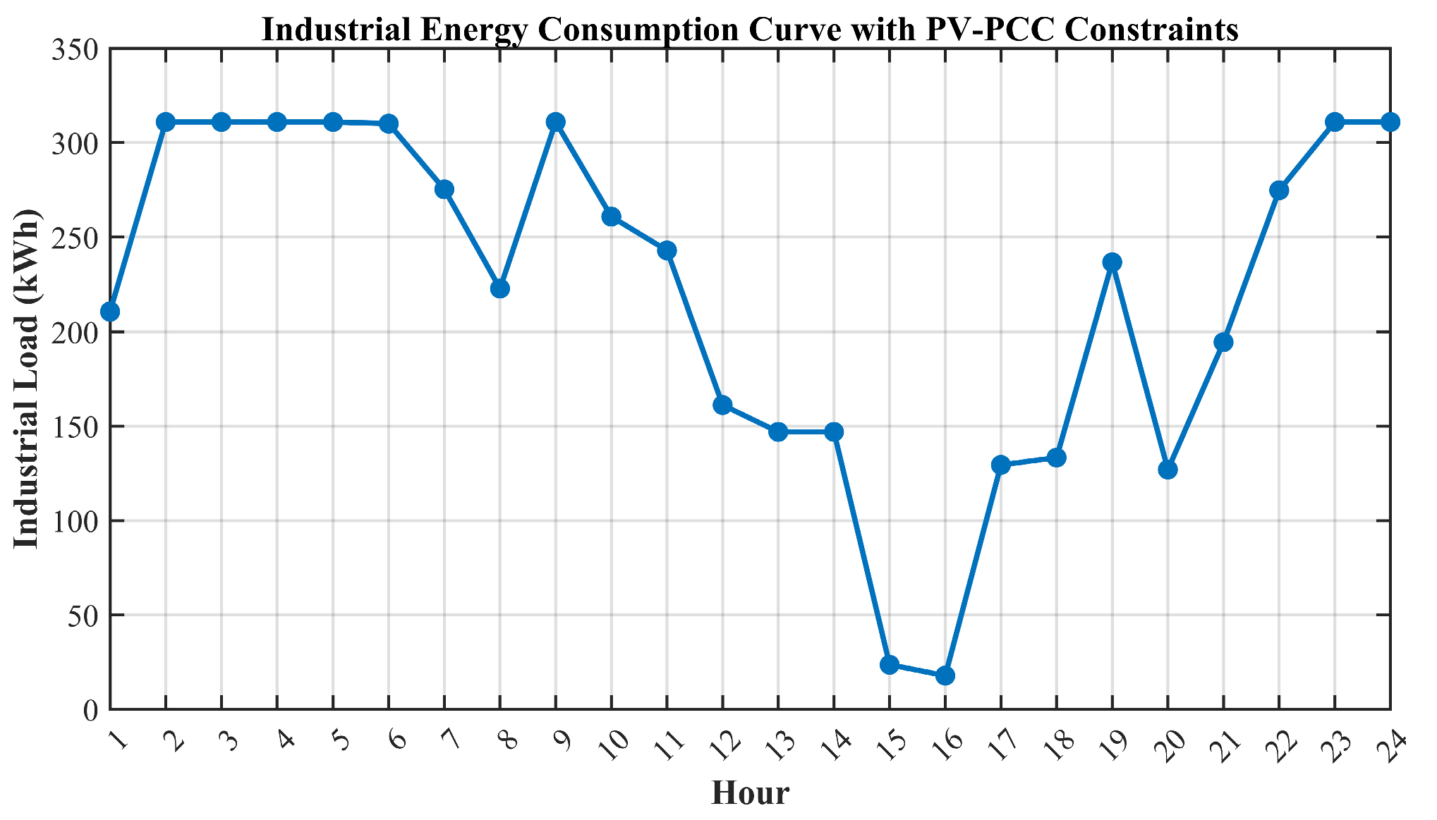
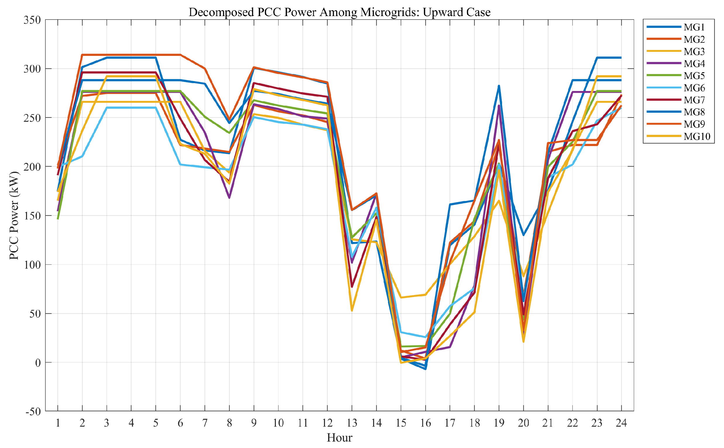
A 24 h dispatch simulation is conducted for a representative industrial microgrid. The results confirm that the incorporation of microgrid operational constraints does not compromise model feasibility. Moreover, the resulting load profile shown in Figure 2 remains fully consistent with the underlying production requirements, demonstrating the applicability of the LSTN framework to industrial microgrid dispatch problems.

4.2. Simulation Setup

A steel powder manufacturing process is selected as the representative industrial application. The production line consists of multiple sequential tasks, including reduction, atomization, dehydration, drying, separation, crushing, classification, and mixing. Material dependencies and intermediate storage buffers are explicitly modeled through the LSTN framework. Detailed process parameters and buffer capacities are adopted from [12].

For each production buffer, the initial inventory is set to 50% of its storage capacity. The inventory of the final product is initially zero. A net production target of 270 t over the 24 h scheduling horizon is imposed, corresponding to an average production rate of 15 t/h.

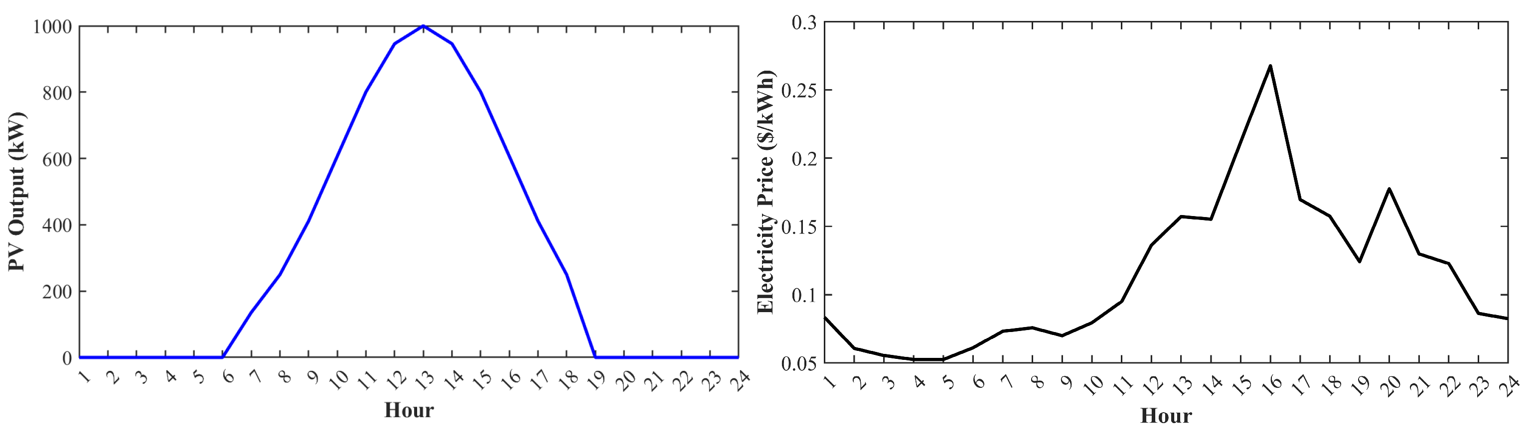
The installed PV capacity of each industrial microgrid is determined according to its average production load. Unless otherwise specified, a representative microgrid is equipped with a 1 MW PV system. The PV generation profile follows a typical clear-sky pattern, and the day-ahead PV forecast profile is treated as a given deterministic input in the optimization model.

Electricity prices are obtained from the PJM Interconnection (PJM) market and correspond to actual locational marginal price data with an hourly resolution. The scheduling horizon is 24 h with a dispatch interval of 1 h. The hourly PV output and electricity price of the PJM market in August 2022 are illustrated in Figure 3.

4.3. Aggregated Flexibility Boundary Identification

Having verified the feasibility of the LSTN model for a single industrial microgrid, this paper further constructs an aggregation of 10 industrial microgrids, with equipment parameters uniformly distributed between 0.8 and 1.2 times the baseline values given in

Table 2. Aggregated adjustable energy under different demand response windows.

DR Window	Time Period	Downward Adjustable Energy (kWh)	Upward Adjustable Energy (kWh)
W1	02:00–05:00	9292	8
W2	09:00–12:00	7489	1891
W3	13:00–16:00	2551	7575
W4	19:00–22:00	5423	3934

. The OALM model established in Section 3 is then used to identify the flexible boundaries of the aggregated industrial load. Unlike virtual-battery models, the OALM model in this paper targets the aggregated industrial production load rather than the PCC net load. For each industrial microgrid, PV output and PCC exchange power serve only as operational constraints and are not objects of demand response tracking.

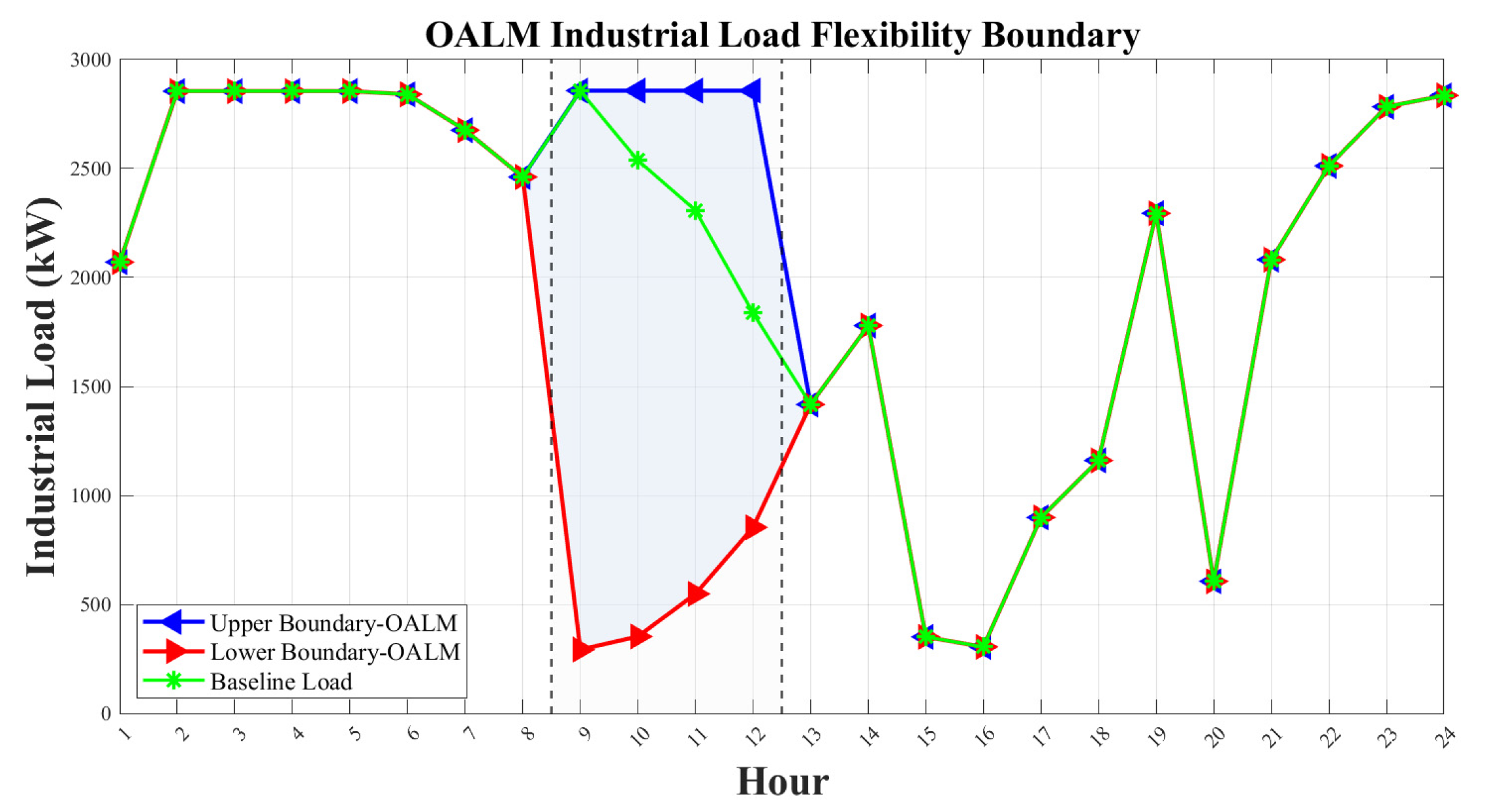
The demand response period is set from 9:00 to 12:00, covering four dispatch intervals. By minimizing and maximizing the aggregated industrial load within each demand response period, the lower and upper power boundaries of the OALM model are obtained. Figure 4 shows the identified flexible boundaries of the aggregated industrial load for the 10 microgrids.

4.4. Coordinated Dispatch Performance Evaluation

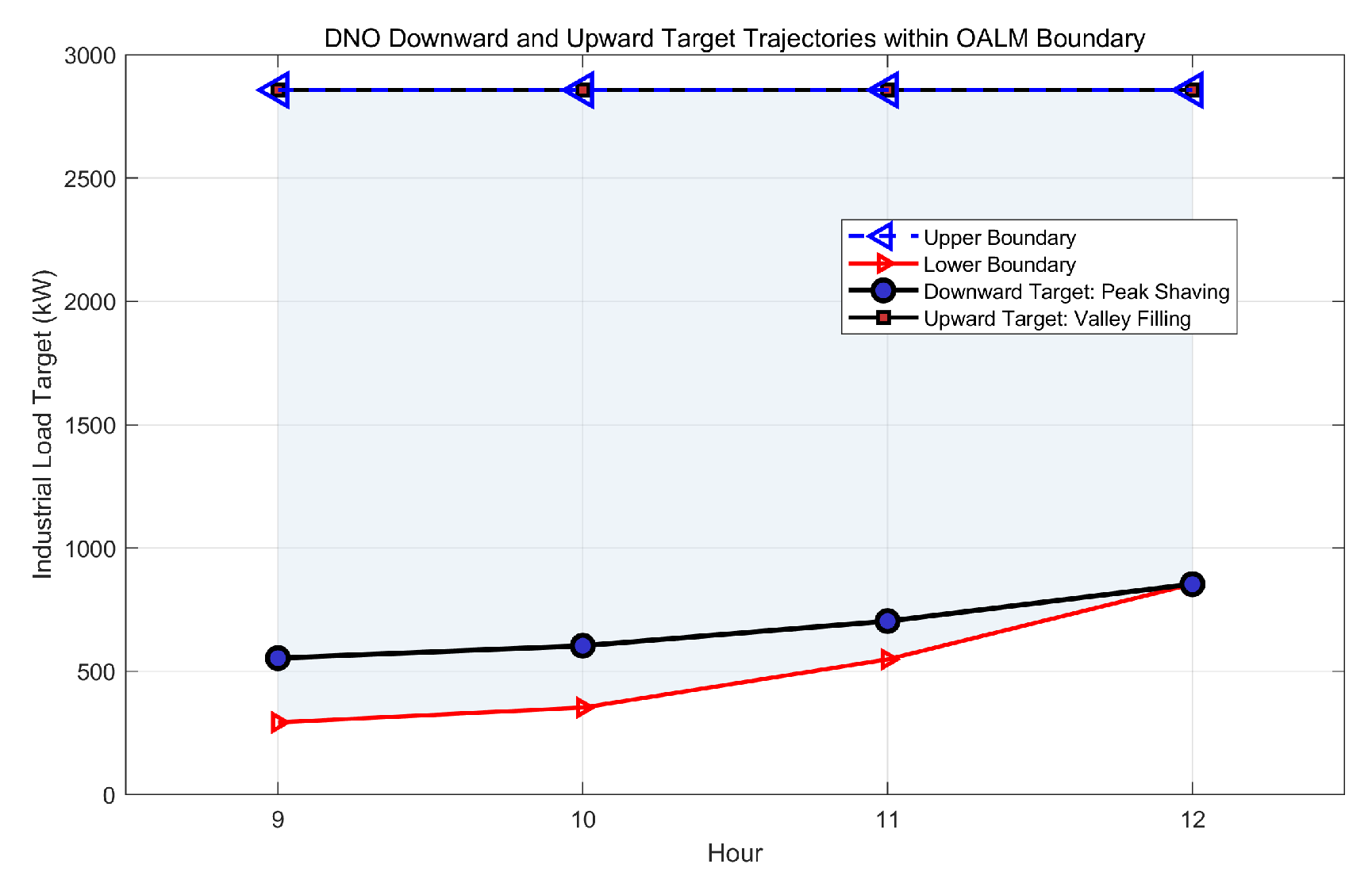
Two types of demand response scenarios are considered: downward regulation and upward regulation, both during the 9:00–12:00 period. The resulting downward and upward targets are shown in Figure 5.

As shown in Figure 5, the downward target lies near the lower OALM boundary, while the upward target lies near the upper OALM boundary. Therefore, the upward target can maximize the aggregated industrial-load power without introducing an additional smoothing penalty and consequently coincides with the upper boundary. The blue triangular markers representing the upper boundary thus overlap with the black square markers representing the upward target. Both targets fall within the identified OALM boundaries, indicating that the DNO-generated target trajectories satisfy the adjustable capability constraints of the aggregated industrial load.

Figure 6 shows the industrial load curves after the aggregator executes the dispatch. The results perfectly match the DNO’s downward target, demonstrating that the aggregator can accurately decompose and execute the industrial load targets issued by the DNO.

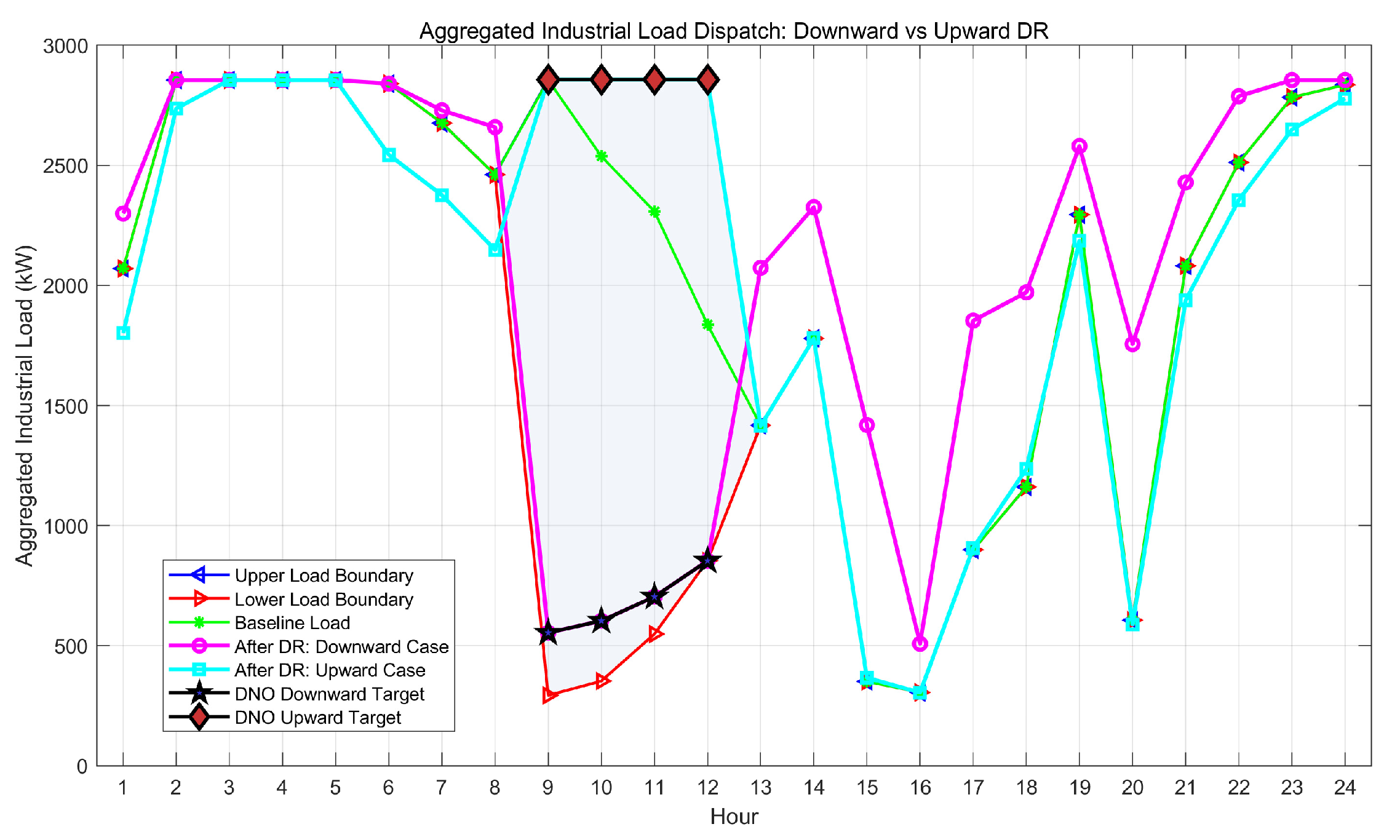
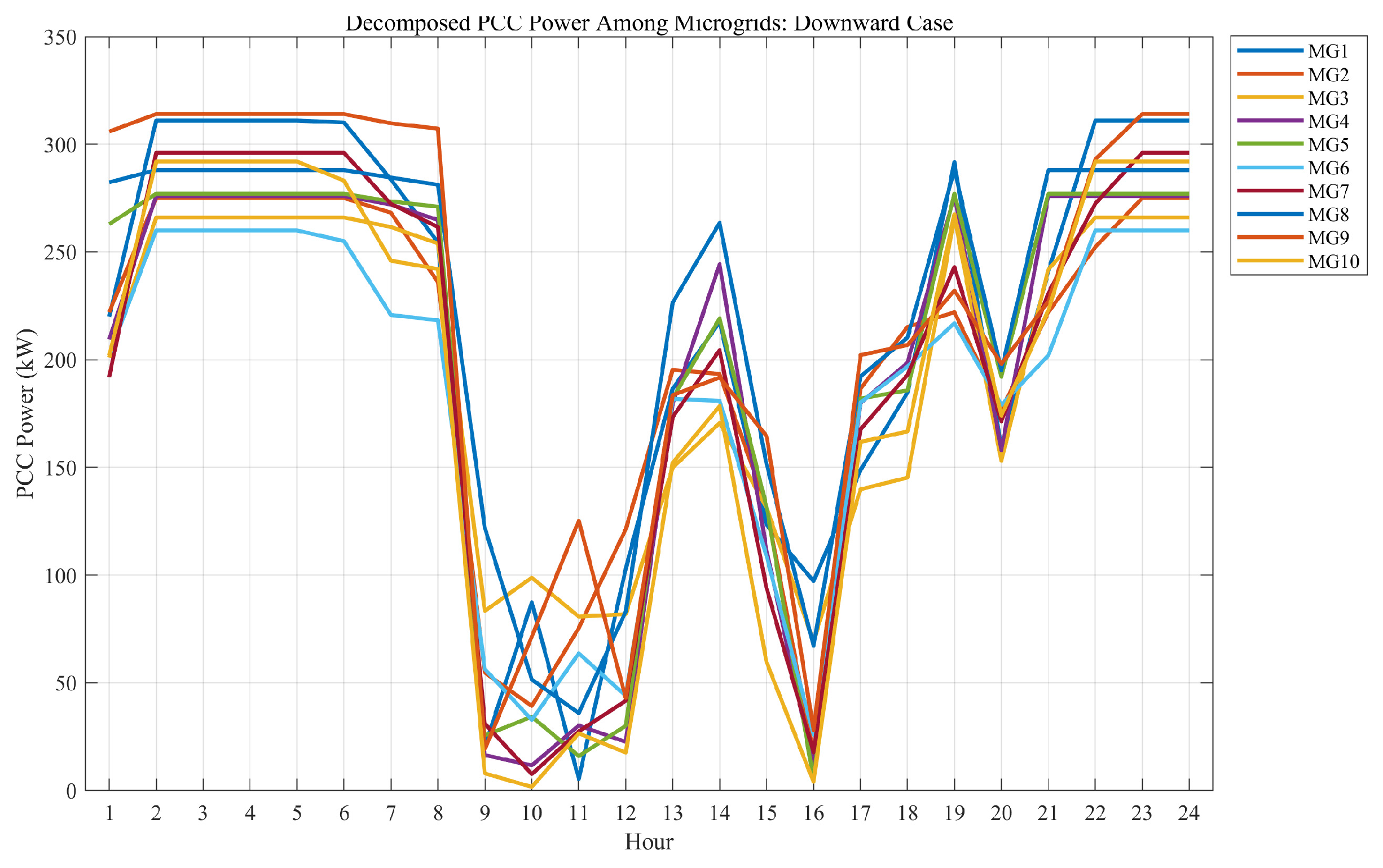
After obtaining the DNO target trajectory, the aggregator further decomposes the target into the 10 individual industrial microgrids and solves the industrial load dispatch problem for both downward and upward scenarios. The resulting aggregated industrial load curves are shown in Figure 7 and Figure 8.

As can be seen from the figures, the dispatched aggregated industrial load remains within the OALM flexible boundaries in both scenarios, confirming that the OALM boundaries provide an effective feasible region constraint for both DNO target generation and aggregator dispatch execution.

4.5. Production Feasibility Verification

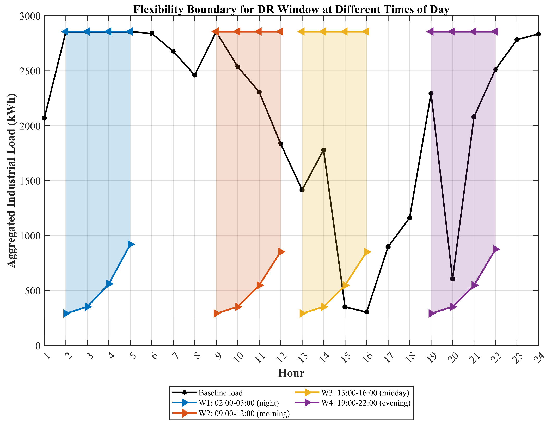
To further verify the ability of the proposed time-varying OALM model to characterize the aggregated flexibility of industrial microgrid clusters, the demand response event duration is kept unchanged at 4 h, while the DR window is shifted to four different periods: nighttime, morning, noon, and evening.

Figure 9 shows the aggregated industrial load flexible boundaries and the upward/downward adjustable energy quantities for each DR window.

As shown in Figure 9, the flexible boundaries of the same industrial microgrid cluster vary significantly across different DR windows. In the nighttime window W1, the baseline aggregated industrial load is close to the upper boundary, leaving very little upward regulation room but substantial downward capacity. In the noon window W3, the baseline load is relatively low, resulting in significantly larger upward regulation space and reduced downward capacity. The evening window W4 exhibits relatively balanced bidirectional regulation capability.

4.6. Sensitivity Analysis Under PV and PCC Constraints

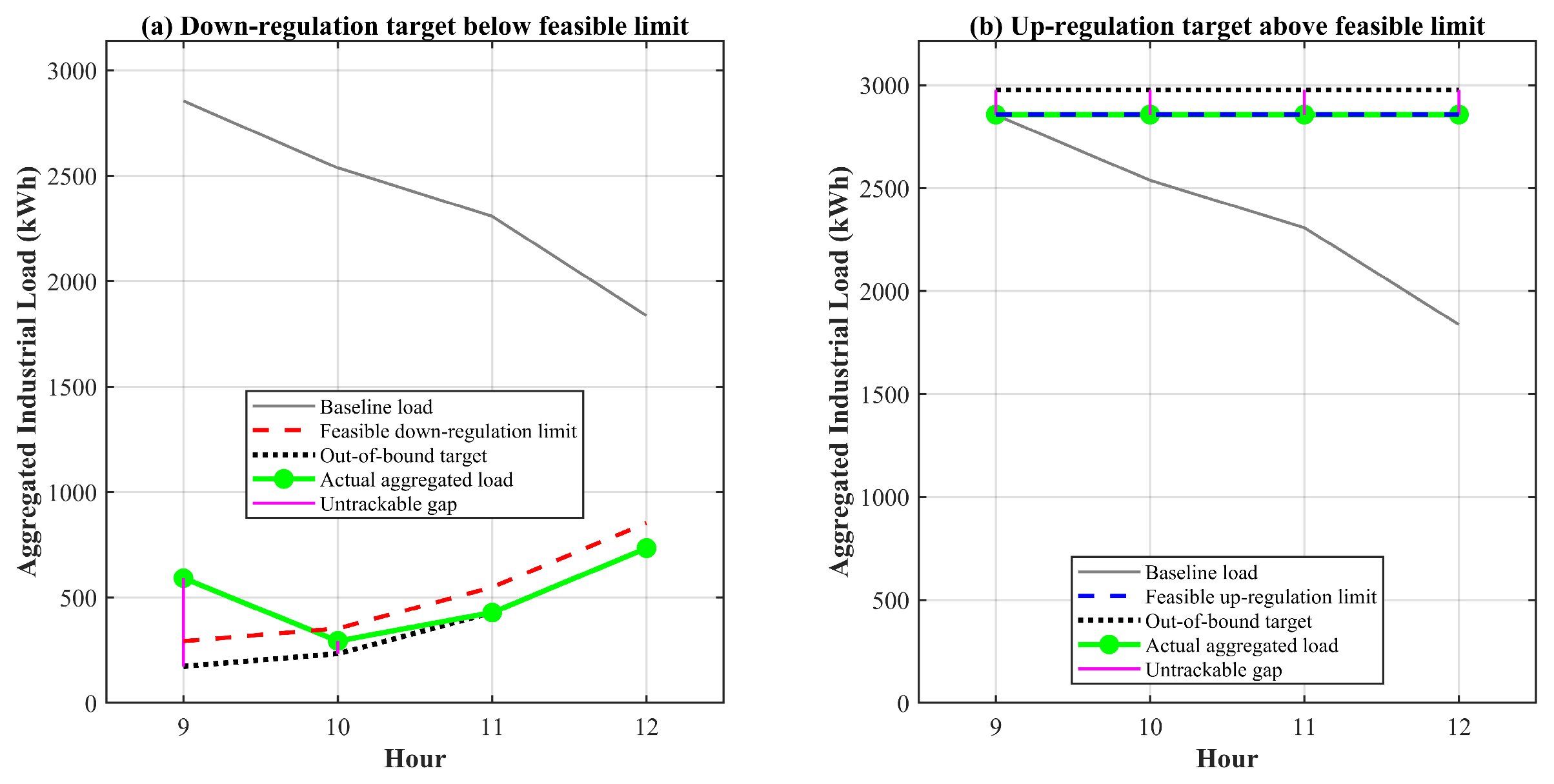
To further verify the robustness of the proposed baseline-free absolute power target tracking model when the target is infeasible, a boundary violation scenario is constructed. In this scenario, the distribution network deliberately issues target power trajectories that exceed the adjustable capability boundaries of the industrial microgrid cluster, and the actual dispatch response of the aggregator is examined.

It should be noted that this paper does not directly use the upper and lower power boundaries sequentially identified by OALM as “absolute limits.” Instead, the lower and upper boundary trajectories from OALM are first fed separately into the aggregator dispatch model as targets, yielding the actually achievable lower and upper limit trajectories of the industrial microgrid cluster under multi-period simultaneous regulation constraints. These are denoted as $P_t^{\mathrm{floor}}$ and $P_t^{\mathrm{ceil}}$, respectively. On this basis, two types of boundary-violating targets are constructed: $P_{t,\mathrm{down}}^{\mathrm{tar}}{P}_t^{\mathrm{floor}}-\Delta P$ and $P_{t,\mathrm{up}}^{\mathrm{tar}}{P}_t^{\mathrm{ceil}}+\Delta P$.

As shown in Figure 10a, in the downward violation scenario, the DNO-issued target power is lower than the achievable lower limit of the industrial microgrid cluster. Consequently, the aggregator cannot fully track the target. However, instead of causing infeasibility or meaningless fluctuations, the actual aggregated industrial load operates stably along the achievable lower limit trajectory. Similarly, in Figure 10b, for the upward violation scenario, the DNO target exceeds the achievable upper limit. Again, the actual aggregated industrial load does not become infeasible but instead tracks the achievable upper limit trajectory.

4.7. Production Executability Analysis Under Extreme Regulation

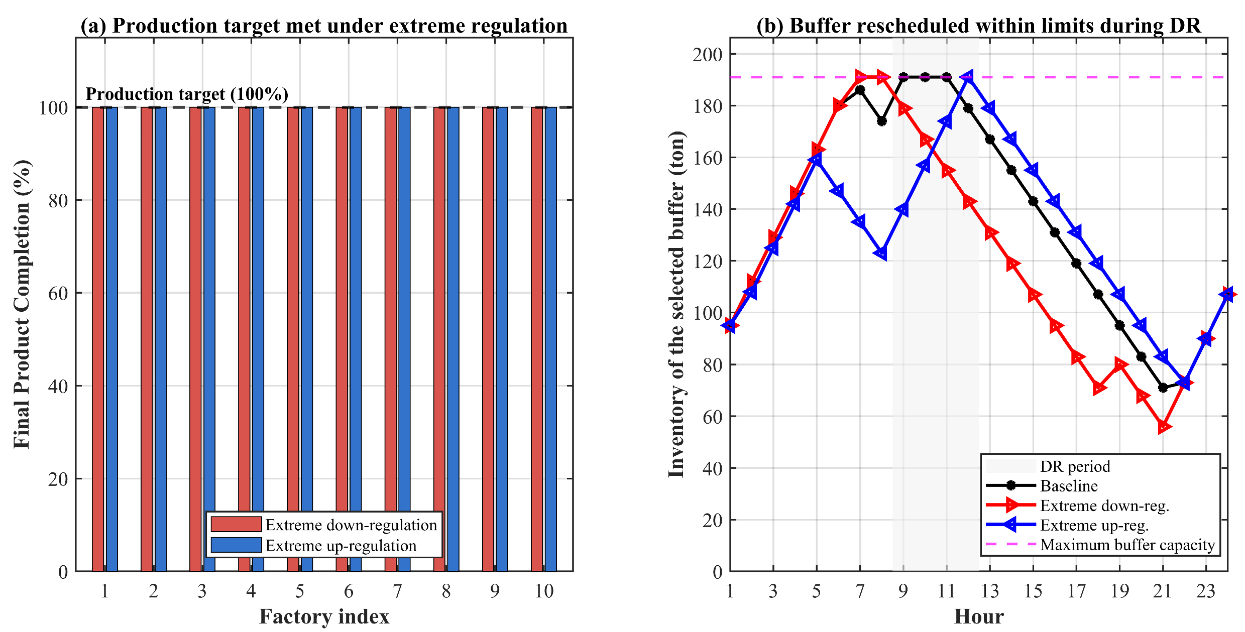
To verify the production executability of the OALM-identified flexible boundaries, extreme regulation scenarios are further constructed. Specifically, the distribution network target power is set to the lower and upper boundary trajectories identified by OALM and compared with the baseline scenario. The key objective is to examine whether the industrial microgrid cluster can still meet the end-of-period production targets while being pushed to its adjustable capability boundaries.

Three scenarios are considered: (1) baseline, where the baseline industrial load serves as the target; (2) extreme downward regulation, where the OALM lower boundary trajectory serves as the target; and (3) extreme upward regulation, where the OALM upper boundary trajectory serves as the target. In each scenario, the aggregator coordinates the dispatch of 10 industrial microgrids, and the final product completion rate of each factory as well as the inventory variations of key intermediate buffers are recorded.

Figure 11a further validates the above conclusion from the perspective of individual factories. It can be seen that, under both extreme downward and extreme upward regulation, the final product completion rate of all factories remains stable at 100%. Figure 11b shows the inventory variations of a selected intermediate buffer under the three scenarios. The results indicate that, during the demand response period, the inventory trajectories are significantly rescheduled across different scenarios, demonstrating that industrial load regulation is indeed achieved through buffer inventory adjustments and task timing reallocation. Nevertheless, under all scenarios, the inventory always satisfies $0\le S_{n,t}^f\le S_n^{f,\max }$, with no instances of negative inventory or buffer capacity violations.

4.8. Model Adaptability Analysis

To further verify the adaptability of the proposed model under source-side fluctuations and varying grid-connection constraints, two special operating scenarios are constructed. The first is a composite scenario involving a sudden PV drop combined with grid-connection limitations, used to analyze the impact of source-side fluctuations on the aggregated flexible boundaries of industrial microgrid clusters. The second is a PCC capacity limitation scenario, used to analyze the tracking capability of industrial microgrid clusters for upward targets under local distribution network congestion.

(1)

Flexible Boundary Changes

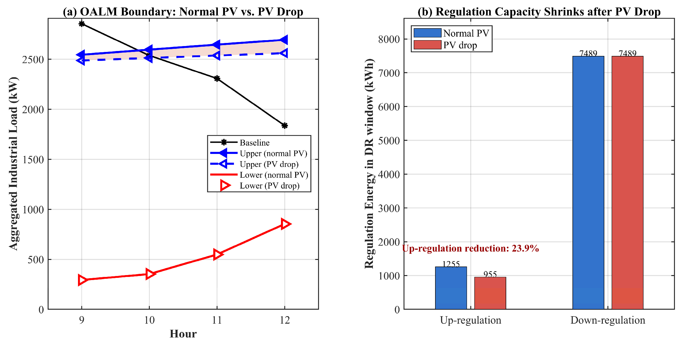
The demand response window is set from 9:00 to 12:00. Within this window, PV output is reduced by 50%, and the maximum PCC exchange power is simultaneously limited to 85% of each factory’s maximum production load. This allows analysis of the impact of PV fluctuations on OALM flexible boundaries under grid-connection constraints.

As shown in Figure 12a, under the PV drop scenario, the lower boundary of the aggregated industrial load remains largely unchanged, while the upper boundary decreases significantly. Figure 12b further shows that under normal PV conditions, the upward adjustable energy is 1255 kWh; after the PV drop, it falls to 955 kWh, a reduction of 23.9%. In contrast, the downward adjustable energy remains at 7489 kWh in both scenarios, essentially unchanged.

The above results indicate that, under grid-connection constraints, a sudden PV drop significantly compresses the upward flexibility of the industrial microgrid cluster, while having little impact on the downward flexibility. This demonstrates that although source-side fluctuations do not directly enter the feasible region of the industrial production load, they can indirectly alter the aggregated flexible boundaries through PCC constraints.

(2)

Target Tracking Performance

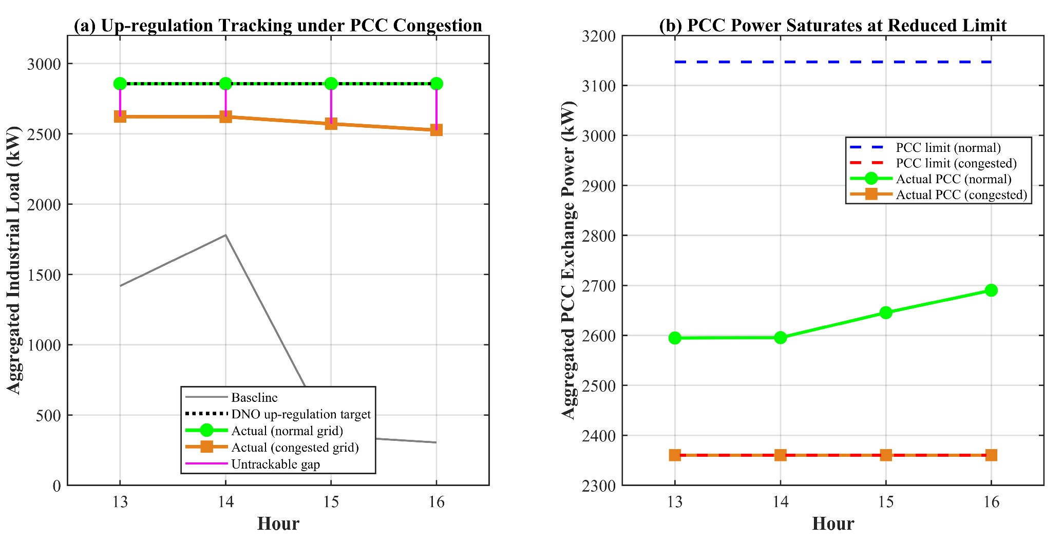
This subsection further considers the issue of PCC capacity tightening due to local feeder congestion in the distribution network and analyzes its impact on the target tracking performance of the industrial microgrid cluster. Given that during the 9:00–12:00 period the baseline industrial load is already close to its upward limit, making it difficult to clearly observe the phenomenon of “upward target being blocked by grid-connection constraints,” the period 13:00–16:00 is instead selected as the congestion window. Within this window, the maximum PCC exchange power is uniformly reduced by 25%.

As shown in Figure 13a, under normal grid-connection conditions, the industrial microgrid cluster can fully track the upward target issued by the DNO. In contrast, under grid-connection limitations, the actual aggregated industrial load is reduced. Figure 13b further shows that under the constrained scenario, the aggregated PCC exchange power remains at the tightened upper limit throughout the congestion period. This result indicates that the direct cause of incomplete target tracking is not the inherent inflexibility of the production process, but rather the limited grid-connection capacity on the distribution network side, which prevents the industrial microgrid cluster from increasing PCC exchange power to support higher industrial production loads.

4.9. Computational Complexity and Scalability Analysis

Since each additional industrial microgrid introduces an independent set of LSTN variables and constraints, the numbers of variables and constraints increase approximately linearly with the cluster size. The simplified models are solved directly without an algorithm-level outer iteration, although the practical solution time may increase nonlinearly because of the enlarged coupled optimization problem.

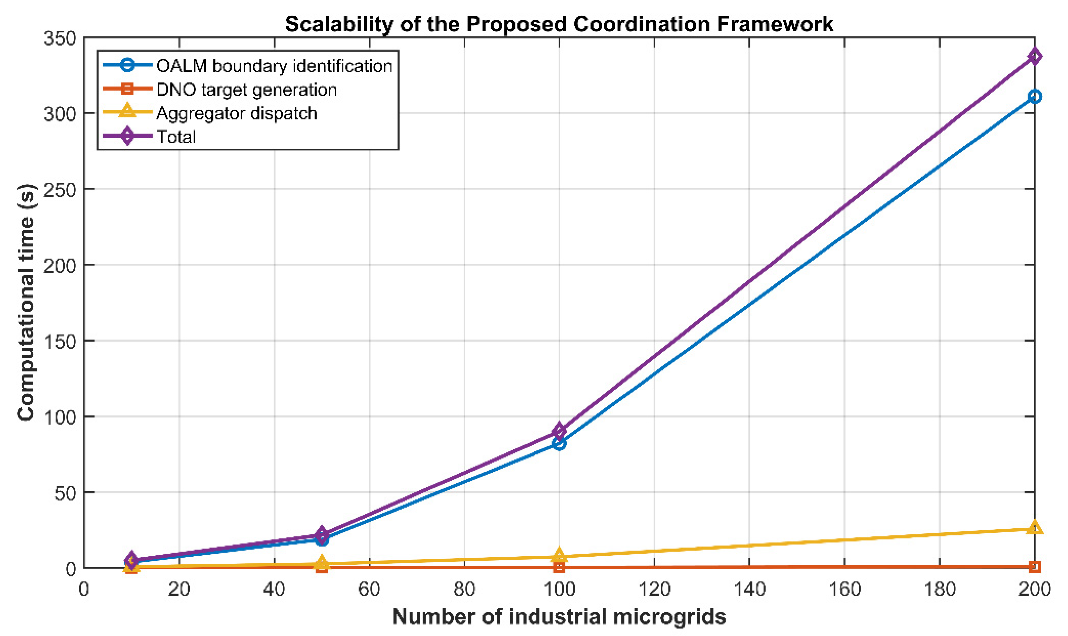
To evaluate the scalability of the proposed framework for industrial microgrid clusters, additional tests are conducted with 10, 50, 100, and 200 industrial microgrids. The computation time of OALM boundary identification, DNO target generation, and aggregator dispatch is reported separately.

Table 3. Computation time and tracking error under different cluster sizes.

N	OALM (s)	DNO (s)	Dispatch (s)	Total (s)	Max Error (kW)
10	4.029	0.257	0.791	5.078	~0
50	18.831	0.288	2.682	21.801	~0
100	82.136	0.445	7.445	90.027	~0
200	310.87	0.785	25.743	337.40	~0

and Figure 14 present the computation results under different cluster sizes. The total computation time increases from 5.08 s to 337.40 s when the number of microgrids increases from 10 to 200. OALM boundary identification is the dominant computational component, whereas DNO target generation and aggregator dispatch remain computationally efficient. The maximum tracking error remains within numerical tolerance for all tested scales, and the dispatch results satisfy the full LSTN production constraints, indicating that the proposed framework is applicable to large-scale industrial microgrid clusters.

4.10. Quantitative Comparison with the Baseline-Based Virtual-Battery Method

To verify the advantage of the proposed baseline-free coordination strategy over conventional baseline-based methods, a traditional VB method is constructed as a benchmark. The VB method represents the regulation instruction as a power deviation from an estimated baseline, whereas the proposed method identifies flexibility boundaries and tracks the target directly in the absolute industrial-load space.

Table 4. Comparison between the proposed method and baseline-based VB.

Method	Base Err (%)	RMSE (kW)	Total (s)	Cost	Util (%)	Completion
OALM	~0	~0	4.284	4589.71	49.90	1.00
Baseline VB	−10	241.30	3.157	4667.41	62.64	1.00
Baseline VB	−5	120.65	3.108	4627.08	56.27	1.00
Baseline VB	~0	~0	3.063	4589.71	49.90	1.00
Baseline VB	5	120.65	3.093	4553.78	43.53	1.00
Baseline VB	10	241.30	3.062	4522.19	37.19	1.00

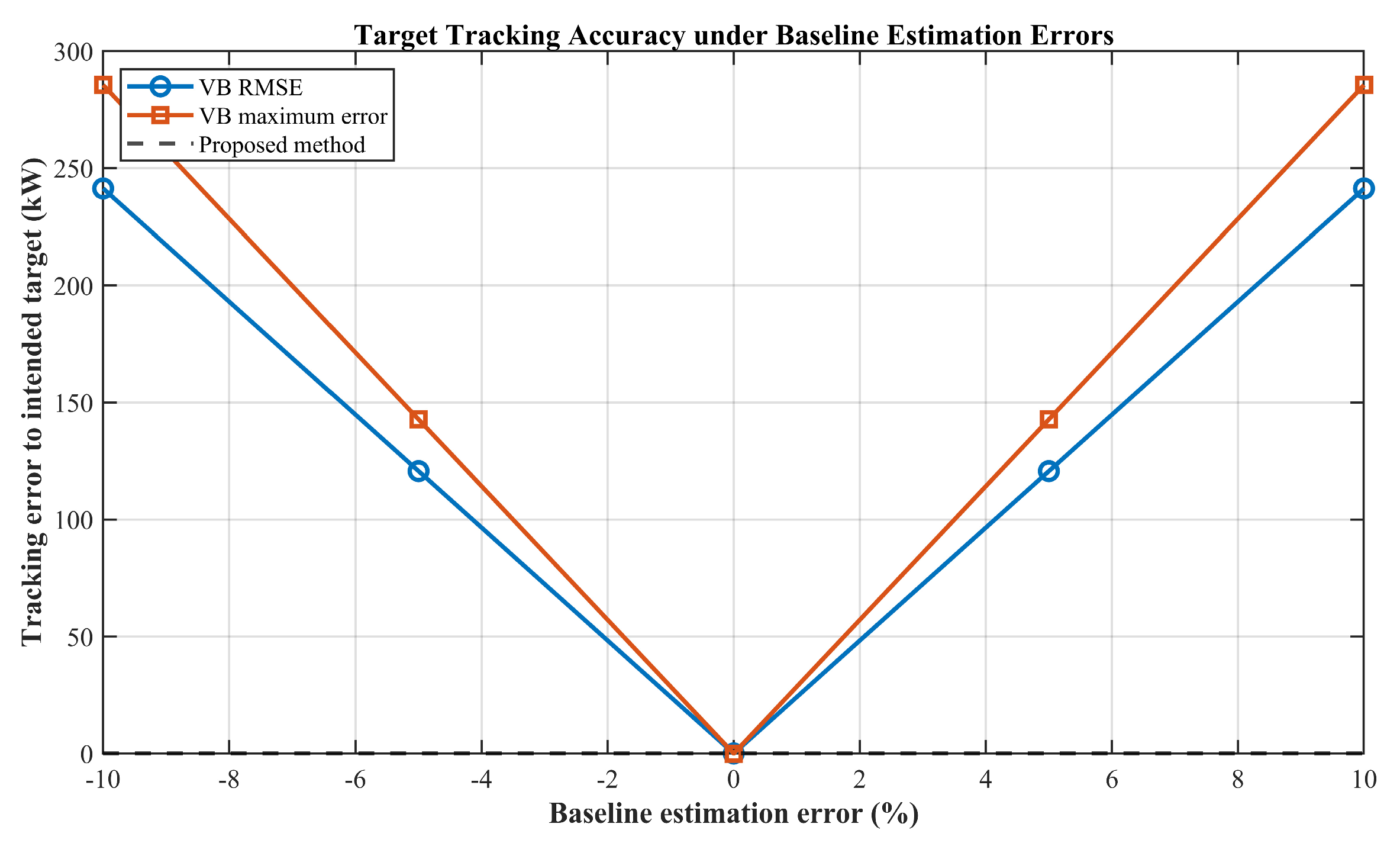
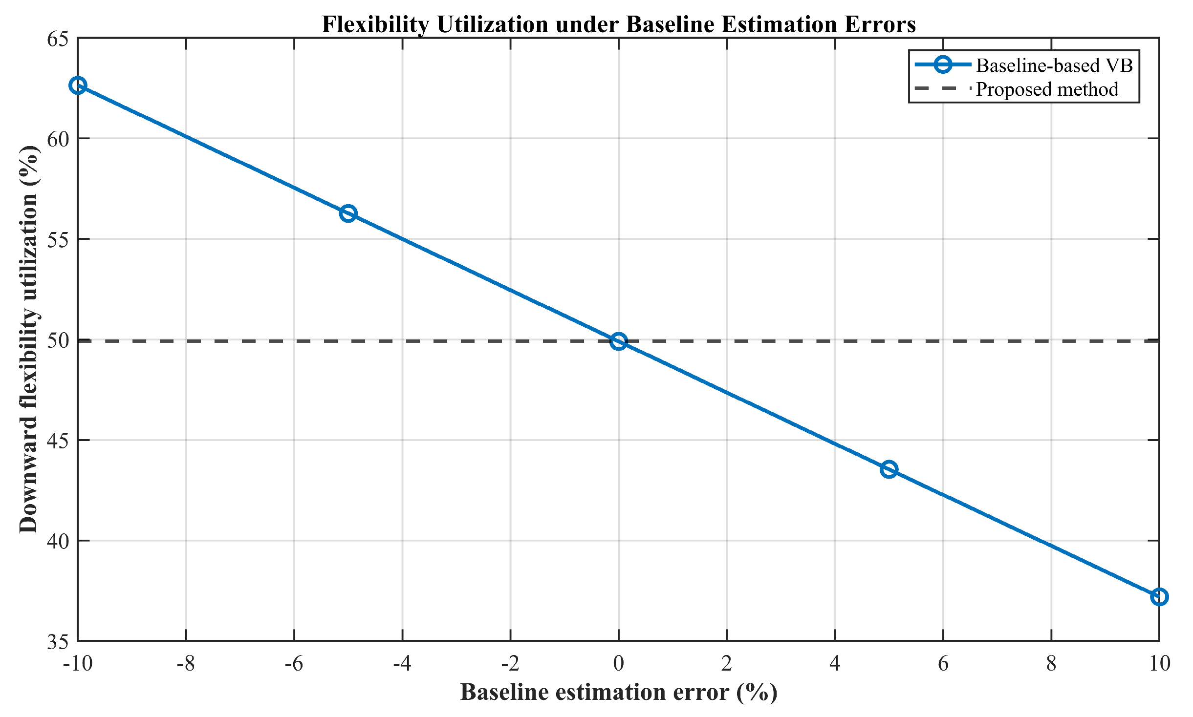
compares the proposed method and the conventional baseline-based VB method in terms of tracking accuracy, computation time, flexibility utilization, and electricity transaction cost. Figure 15 and Figure 16 further show the effects of baseline estimation errors on tracking error and flexibility utilization. When the baseline estimation error is ±5% and ±10%, the RMSE of the VB method with respect to the intended absolute target reaches 120.65 kW and 241.30 kW, respectively, while the tracking error of the proposed method remains within numerical tolerance. These results indicate that baseline errors significantly affect the actual tracking performance of conventional VB-based coordination, whereas the proposed method avoids the propagation of baseline estimation errors.

For economic performance, Table 4 reports the electricity transaction cost calculated using time-of-use prices and PCC exchange power. It should be noted that the lower cost observed for the VB method under positive baseline errors is caused by target deviation and insufficient flexibility activation, and therefore does not indicate better economic performance under the same intended target. Economic performance should thus be interpreted together with tracking accuracy.

4.11. Comparative Performance Evaluation and Sensitivity Analysis

The comparison with the conventional baseline-based VB method has been presented in the preceding subsection. This subsection further compares the proposed method with a production-agnostic aggregation model and analyzes the sensitivity of the results to key parameter settings.

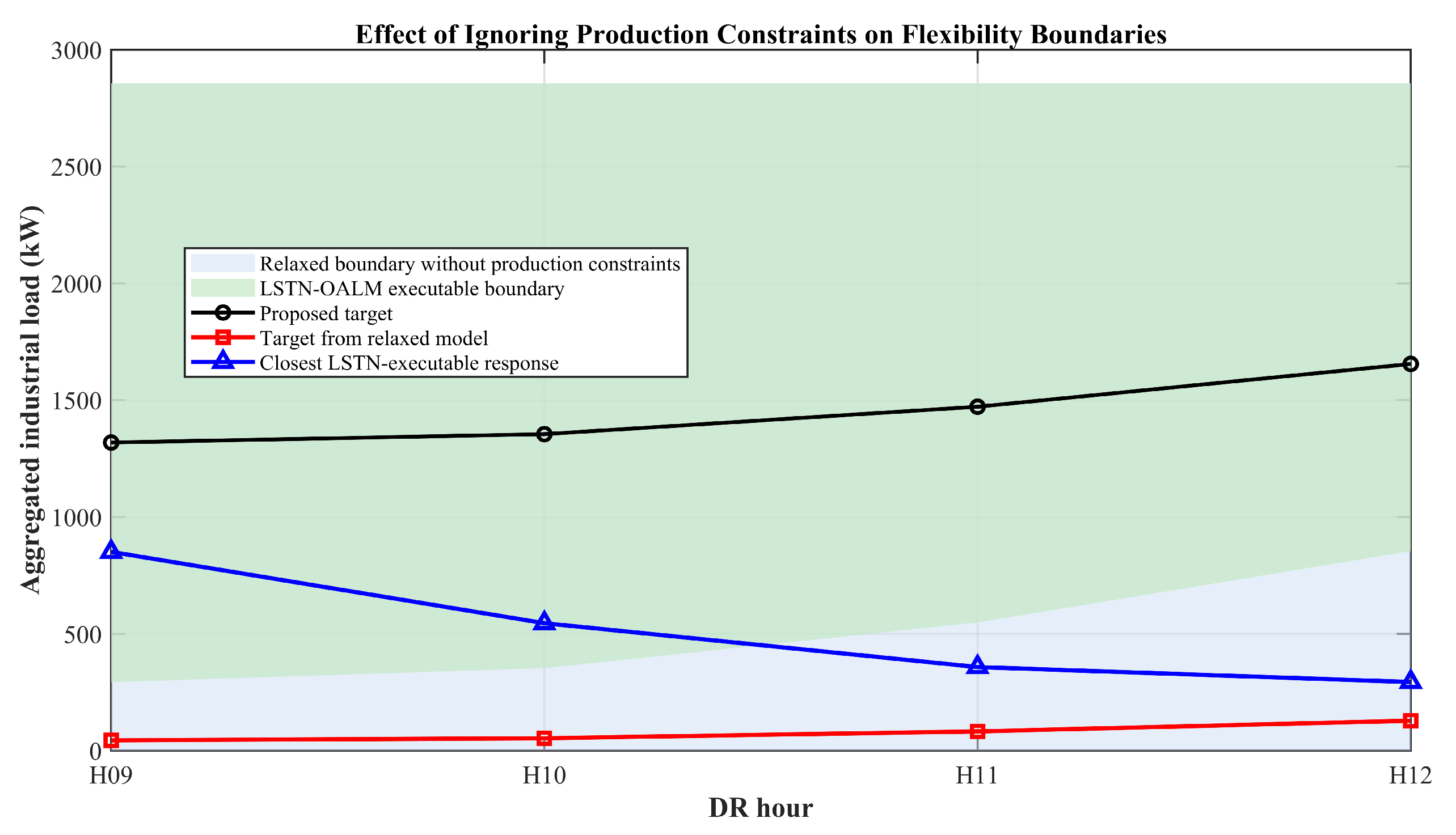
To further demonstrate the necessity of production-process constraints in industrial load aggregation, a production-agnostic power-energy aggregation model is constructed as a benchmark. This model only considers hourly industrial-load limits, PV availability, and PCC exchange constraints, while ignoring material balance, inventory capacity, and terminal production requirements.

Table 5. Boundary comparison between LSTN-OALM and production-agnostic aggregation.

Model	Width (kWh)	Expansion (%)	Upper over (kWh)	Lower over (kWh)	Boundary Time (s)
Proposed LSTN-OALM	9379.90	0	0	0	3.789
No-production model	11,428.00	21.84	~0	2048.10	0.727

and Figure 17 compare the flexibility boundaries obtained by the LSTN-OALM and the production-agnostic model. The results show that ignoring production constraints expands the boundary width from 9379.90 kWh to 11,428.00 kWh, corresponding to a 21.84% expansion. The downward regulation capability is overestimated by 2048.10 kWh.

Table 6. Executability check of the production-agnostic target.

Method/Target	RMSE (kW)	Max Err (kW)	Dispatch (s)	Cost	Util (%)	Completion	Exact Feasible
Proposed LSTN-OALM	~0	~0	0.464	4589.71	49.90	1.00	1
No-production aggregation	~0	~0	0.149	−254.71	123.25	-	0
No-production target under LSTN	499.16	806.72	0.382	4987.95	100.01	1.00	0

further reports the executability check of the production-agnostic target under the full LSTN production constraints. All dispatch schedules evaluated under the complete LSTN production constraints achieve 100% terminal production completion, with zero inventory-constraint violation. These production-executability metrics are not applicable to the standalone production-agnostic aggregation model because material-balance, inventory-capacity, and terminal-production constraints are excluded from that model. Although the relaxed model can track its own target with zero error, the target is not exactly executable under the full LSTN production constraints; the checked LSTN dispatch has an RMSE of 499.16 kW and a maximum error of 806.72 kW. Therefore, using only power–energy boundaries without production-process constraints may lead to overestimated flexibility and non-executable dispatch targets.

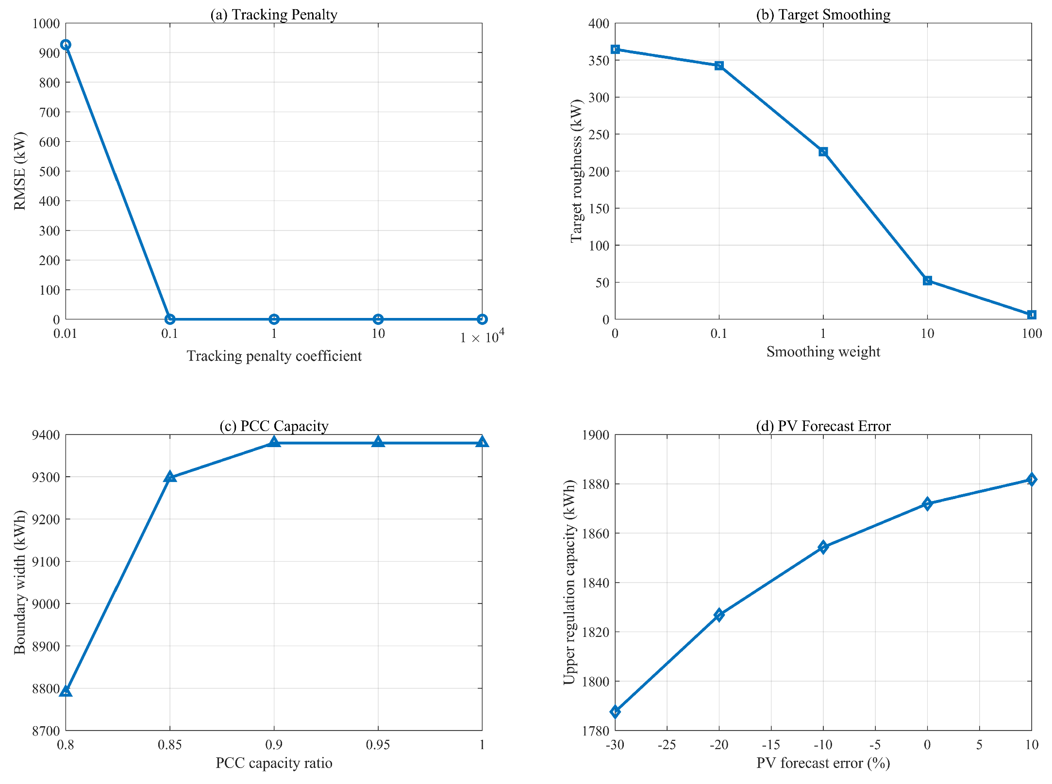
To analyze the impact of key parameters, sensitivity analyses are further conducted, as shown in

Table 7. Sensitivity to tracking penalty coefficient.

Penalty	RMSE (kW)	Max Err (kW)	Dispatch (s)	Util (%)	Completion	Inv. Viol.
0.01	927.08	1280.08	0.442	5.44	1.00	~0
0.1	~0	~0	0.487	49.90	1.00	~0
1	~0	~0	0.435	49.90	1.00	~0
10	~0	~0	0.455	49.90	1.00	~0
10,000	~0	~0	0.465	49.90	1.00	~0

,

Table 8. Sensitivity to DNO target smoothing weight.

Smooth Weight	Roughness (kW)	Energy (kWh)
0	364.44	5331.06
0.1	342.59	5331.06
1	226.41	5331.06
10	52.15	5331.06
100	6.00	5331.06

,

Table 9. Sensitivity to PCC capacity ratio.

PCC Ratio	Up Cap (kWh)	Down Cap (kWh)	Width (kWh)	RMSE (kW)	Completion
1	1890.89	7489.01	9379.90	~0	1.00
0.95	1890.89	7489.01	9379.90	~0	1.00
0.9	1890.89	7489.01	9379.90	~0	1.00
0.85	1871.91	7489.01	9297.76	~0	1.00
0.8	1521.29	7489.01	8789.79	~0	1.00

and

Table 10. Deterministic sensitivity to PV output deviation.

PV Deviation (%)	Up Cap (kWh)	Shrink (%)	RMSE (kW)	Completion
−30	1787.61	4.50	~0	1.00
−20	1826.84	2.41	~0	1.00
−10	1854.32	0.94	~0	1.00
0	1871.91	~0	~0	1.00
10	1881.75	−0.53	~0	1.00

and Figure 18. The results show that an overly small tracking penalty coefficient leads to significant tracking deviation; increasing the smoothing weight reduces target trajectory fluctuations; tightening the PCC capacity ratio compresses the flexibility boundary; and negative PV output deviation weakens upward regulation capability. All sensitivity tests maintain 100% production completion and zero inventory constraint violation.

4.12. Validation of Voltage- and Congestion-Constrained Coordination

A representative radial feeder consisting of ten load buses and one upstream substation bus is constructed to evaluate the effects of the added distribution-network constraints. Ten industrial microgrids are connected to the ten load buses through their PCCs. The feeder base capacity is 5 MVA, the substation voltage is 1.0 p.u., the power factor of each industrial microgrid is 0.95, and the allowable voltage range is 0.95–1.05 p.u. The resistance and reactance of each feeder branch are set to 0.016 p.u. and 0.010 p.u., respectively, while the branch capacities are assigned according to their downstream aggregated load levels. The PCC-only formulation and the proposed network-constrained formulation are compared under identical LSTN production parameters, PV output, local PCC limits, and target settings.

Under the PCC-only formulation, ex-post network evaluation gives a minimum bus voltage of 0.9370 p.u. and a maximum branch loading of 123.93%, indicating that a target satisfying the local PCC limits may still violate feeder operating constraints. After incorporating the distribution-network constraints, all bus voltages remain within the allowable range of 0.95–1.05 p.u., and the maximum branch loading does not exceed 100%. The upper cumulative-energy boundary decreases from 11,428.00 kWh to 10,117.12 kWh, representing a reduction of 11.47%. Meanwhile, the target-tracking RMSE remains within numerical tolerance, the production completion rate remains 100%, and no inventory constraint is violated. These results demonstrate that the added network constraints prevent voltage violations and branch congestion while preserving production-process executability.

5. Conclusions

This paper establishes a complete coordinated framework encompassing individual industrial microgrid modeling, aggregated flexible boundary identification via OALM, DNO target generation, and aggregator dispatch tracking. Case studies verify the feasibility and effectiveness of the proposed method. The results show that, while satisfying microgrid operational constraints, the method enables peak shaving, valley filling, and renewable energy accommodation for industrial loads. Furthermore, the OALM boundaries provide actionable power and energy constraints, ensuring reasonable DNO targets and accurate aggregator tracking. This offers a feasible and efficient technical solution for distribution network demand response with strong practical application potential.

However, several limitations remain and should be addressed in future research. First, the current framework is formulated as a deterministic coordination optimization model, in which PV forecasts, production-process parameters, and equipment states are treated as given inputs. Operating uncertainties such as PV forecast errors, communication delays, equipment failures, and unexpected production disturbances are not explicitly considered in the current version. Second, the LSTN model adopted in this paper is mainly applicable to industrial processes whose material conversion relationships and electricity consumption characteristics can be reasonably described by linear models. For strongly nonlinear dynamic production processes, further extensions such as piecewise linearization, mixed-integer nonlinear modeling, or data-driven approximations are required. Third, although a balanced linearized radial power-flow model has been incorporated to represent bus-voltage and branch-capacity constraints, the current network model adopts a fixed power factor and does not consider nonlinear power losses, three-phase unbalance, meshed operation, or full AC power-flow characteristics. Future work will extend the proposed framework by incorporating more detailed three-phase AC network models, rolling optimization, robust or stochastic optimization for operating uncertainties, and practical validation in industrial microgrid clusters and distribution feeders.