Article

Cooperation or Fragmentation? The Impact of Green Innovation Collaboration on Pollution Governance in Inter-Provincial Administrative Boundary Areas: Evidence from China


1
School of International Economics and Trade, Nanjing University of Finance & Economics, Nanjing 210023, China
2
Nuclear Energy Economics and Management Research Center, University of South China, Hengyang 421001, China
*
Author to whom correspondence should be addressed.
Sustainability 2026, 18(17), 8668; https://doi.org/10.3390/su18178668
Submission received: 12 July 2026 / Revised: 10 August 2026 / Accepted: 18 August 2026 / Published: 24 August 2026
(This article belongs to the Special Issue Innovation, Regional Disparities and Sustainable Development)

Abstract

Inter-provincial administrative boundary areas are particularly vulnerable to ineffective regional pollution governance because they are simultaneously affected by transboundary pollution diffusion and administrative fragmentation. Existing governance practices, however, continue to rely heavily on territorially based regulation and administrative coordination, while the potential of cross-regional green-technology collaboration to address boundary pollution has received insufficient attention. Using panel data for Chinese prefecture-level cities from 2011 to 2023, this study systematically examines the impact of green innovation collaboration (GIC) on pollution control in areas along interprovincial administrative boundaries through two-way fixed-effects, instrumental-variable, Heckman two-step, and spatial Durbin models. The results show that, first, GIC significantly reduces pollution in these areas, and this finding remains robust across a range of robustness checks. GIC also generates significant spatial spillovers: while reducing local boundary pollution, it improves air quality in neighboring cities. Second, the heterogeneity analysis indicates that this effect is more pronounced in cities facing greater pollution-control pressure, lower fiscal pressure, and higher levels of openness. The regional results also reveal certain differences. Third, the mechanism analysis shows that cross-regional collaborative governance and industrial upgrading constitute two relatively independent parallel transmission pathways rather than a sequential chain, and their relative contributions vary with city conditions. These findings provide empirical evidence for improving interprovincial collaborative governance, facilitating the cross-regional diffusion of green technologies, and implementing differentiated environmental policies.

1. Introduction

At a critical stage in China’s transition toward a green and low-carbon economy, coordination and fairness in regional environmental governance have become increasingly prominent policy concerns. Yet areas along inter-provincial administrative boundaries have long remained at the margins of environmental regulation and face distinctive pollution-governance difficulties. On the one hand, differences in environmental standards, regulatory intensity, and industrial entry requirements across boundary areas can induce a “pollution haven” effect [1], turning inter-provincial border zones into destinations for highly polluting and energy-intensive industries and deepening structural pollution. On the other hand, under growth competition and territorial regulatory constraints, local governments may weaken pollution control in boundary areas and externalize part of the pollution cost to neighboring jurisdictions, giving rise to free riding, pollution transfer, and buck-passing in governance responsibility [2]. The difficulty of pollution governance in inter-provincial boundary areas therefore arises from the joint effects of transboundary pollution diffusion, administrative fragmentation, and insufficient regional coordination, which make regulatory gaps, externalized responsibility, and ineffective governance more likely. Figure 1 shows that (a) PM2.5 concentrations in China exhibited a clear overall downward trend from 2011 to 2023; (b) PM2.5 concentrations in interprovincial boundary cities remained consistently higher than those in inland cities; and (c) the average difference between the two groups during the sample period was 2.66 μg/m3. Although the gap generally narrowed, it remained positive at 1.2 μg/m3 in 2023. Across the eastern, central, western, and northeastern regions, PM2.5 concentrations in border cities also declined, but the trajectories differed substantially, indicating that pollution governance in inter-provincial boundary areas remains both persistent and heterogeneous. The tension between administrative borders and pollution diffusion is not unique to China. The European Union has used the Interreg program (2021–2027) to invest around €10 billion in a cross-border cooperation framework, while the AIR TRITIA project established common monitoring and management arrangements for air quality in border areas; India and ASEAN have likewise developed institutions for coordinated regional air governance and an agreement on cross-border haze governance. These experiences indicate that transboundary pollution control requires regionally shared information and technologies as well as standing cooperation mechanisms.
The externalities associated with transboundary pollution can be mitigated by lowering the cost of coordination across jurisdictions and establishing effective horizontal negotiation and compensation mechanisms [3,4]. Such arrangements can address the allocation of existing pollution emissions and governance responsibilities, but they focus mainly on pollution control, end-of-pipe treatment, and compensation payments. Their effectiveness still depends on stable negotiation, clear monitoring standards, and enforceable benefit-sharing rules, so they cannot by themselves resolve structural problems such as insufficient green-technology supply in boundary areas, high cross-regional coordination costs, and resistance to industrial transformation [5]. Governance failure at administrative boundaries arises mainly for three reasons. First, pollution information and governance experience are dispersed across jurisdictions, making it difficult to form a shared understanding in time. Second, local governments bear the costs of pollution control while environmental benefits may be shared with neighboring areas, leaving insufficient incentives for joint investment [6]. Third, boundary areas often lack green technologies and innovation resources and therefore cannot independently upgrade clean production and pollution-control facilities [7]. Transboundary pollution governance therefore requires expanding the supply of green technologies, promoting their diffusion and joint application across regions, and improving the capacity of boundary areas to absorb and commercialize these technologies [8].
Traditional studies have focused mainly on environmental regulation or technological innovation within individual regions [9,10,11], overlooking spillovers from interregional knowledge flows and technological collaboration. Recent research on green innovation and air pollution or carbon emissions has expanded from within-region R&D investment to cross-regional joint R&D and application of results [12,13], connecting different innovation actors through collaboration networks. Its mechanisms operate at two levels. The first is technological diffusion and learning. Patent collaboration between developed and boundary areas facilitates the cross-administrative diffusion of advanced technologies for clean production, pollution monitoring, and end-of-pipe treatment, easing the technological lock-in created by weak local R&D capacity in boundary areas [14,15]. The second is interest alignment and policy coordination. Joint R&D requires partners to share funding, bear R&D risks, and share technological returns, thereby creating a cross-regional network of aligned interests. When collaboration extends to governments, firms, and research institutions, the network can provide stable channels for sharing environmental-monitoring information, negotiating governance standards, and conducting joint enforcement. It can reduce information asymmetry and opportunism among local governments and encourage neighboring jurisdictions to adopt more consistent pollution-control arrangements [16]. Green innovation collaboration may therefore improve both the technological capacity for governance in boundary areas and the incentive structure underlying fragmented local governance.
Although existing studies identify the emission-reduction effects of green technological innovation on air pollution, water pollution, and carbon emissions at the regional level [8,12,13], or examine boundary pollution and its governance through cross-regional environmental protection, ecological compensation, and administrative-boundary governance [3,16,17], few place green innovation collaboration and administrative-boundary pollution in a common analytical framework. Micro-level empirical tests based on patent-collaboration networks and geographic boundary information remain particularly limited. Whether green innovation collaboration can reduce pollution intensity in boundary areas and through what mechanisms it does so have not been adequately identified. To address this gap, this study uses panel data for Chinese prefecture-level cities from 2011 to 2023. Pollution is measured by the annual average PM2.5 concentration of each city. Green innovation collaboration is measured by the number of intercity green-technology patent collaborations and green low-carbon patent collaborations. In addition, a continuous index of inter-provincial boundary exposure intensity is constructed using GIS spatial data. Based on these measures, this paper systematically examines the effects and mechanisms of green innovation collaboration on pollution governance in inter-provincial administrative boundary areas.
This study contributes to the existing literature in three main ways. First, it identifies green innovation collaboration as an underexamined channel for mitigating transboundary pollution and distinguishes two separate mechanisms through which it operates: cross-regional collaborative governance and industrial upgrading. In doing so, it moves beyond the conventional emphasis on unilateral environmental regulation and the physical transmission of pollution, thereby advancing the dialog between green economics and economic geography. Second, it shifts the analytical lens to inter-provincial boundary areas, where institutional fragmentation and pollution externalities are most pronounced, and constructs a continuous boundary-exposure intensity index based on GIS data to precisely measure this setting. This design allows us to capture how cross-city knowledge coordination operates precisely in the very spaces where administrative fragmentation has traditionally hindered policy coordination. Third, it adopts a multi-method identification strategy encompassing instrumental variable estimation, the Heckman two-step procedure, and the spatial Durbin model to mitigate endogeneity biases and account for spatial spillover effects, which enhances the reliability of causal inferences. Collectively, these contributions not only deliver novel empirical evidence regarding interprovincial boundary governance in China but also establish a transferable analytical framework for exploring environmental cooperation in other federal or multi-jurisdictional settings.
The remainder of this paper is organized as follows. Section 2 reviews the relevant literature. Section 3 develops the theoretical framework and research hypotheses. Section 4 describes the empirical models, variable measurement, and data sources. Section 5 presents and discusses the empirical results. Finally, Section 6 summarizes the main conclusions and offers policy recommendations.

2. Literature Review

2.1. Pollution Governance in Interprovincial Administrative Boundary Areas

Early studies drew on environmental federalism and transboundary externalities, understanding boundary pollution as a governance failure caused by a mismatch between the natural reach of pollutant diffusion and administrative management boundaries [5,18]. Air pollution has clear spatial-transport characteristics: its effects spread differently with wind direction and distance, so pollution damage is not confined to the place of emission [19]. Under territorial regulation, local governments generally bear responsibility for environmental governance within their jurisdictions, while the costs of transboundary pollution may be shared by neighboring areas. This creates scope for free riding and weaker enforcement at boundaries [20]. Research in China further emphasizes that an inter-provincial administrative boundary is not merely a geographic line; it is also an institutional boundary where environmental-regulatory responsibility, industrial entry rules, and performance incentives are fragmented [6,21]. When environmental-regulation intensity and pollution-control costs differ across areas, pollution-intensive firms may relocate to jurisdictions with lower compliance costs [22]. In inter-provincial boundary areas, large air-polluting firms are more likely to locate near provincial borders on the downwind side, suggesting that local governments may strategically use the spatial placement of polluting firms to shift part of the environmental cost to neighboring areas [23]. Pollution governance in inter-provincial boundary areas therefore concerns the combined management of transboundary externalities, fragmented territorial regulation, and insufficient regional coordination. In terms of measurement, existing studies generally treat administrative boundaries as either a discrete identifier or a continuous spatial variable. Some use a boundary-area dummy to classify cities near provincial, county, or other administrative borders as boundary observations. This approach is intuitive but cannot capture differences in the intensity of boundary exposure across cities [24]. Others use the distance from monitoring stations, firms, or counties to the nearest administrative boundary, or distance to a downwind boundary, to construct continuous measures of proximity and gradient effects [23,25]. Subsequent work has examined how boundary pollution is formed. Differences in economic development and industrial structure alter the spatial flow of polluting industries. Areas with lower environmental costs and weaker regulatory capacity are more likely to receive energy-intensive and high-emission industries, reinforcing pollution concentration at boundaries [26]. Under growth competition and fiscal incentives, local governments may attract industries through land supply, tax preferences, or regulatory flexibility. Differences in enforcement and industrial-entry policies then affect the location choices of polluting firms [27,28]. At the same time, weak cross-provincial enforcement coordination, incomplete ecological-compensation mechanisms, and inadequate pollution-information sharing and joint-monitoring systems weaken the internalization of transboundary externalities, leaving boundary areas more vulnerable to regulatory gaps and responsibility shifting [29].
Overall, existing studies have developed a research line from identifying transboundary pollution externalities and analyzing strategic behavior by local governments and firms to coordinating environmental regulation and designing ecological-compensation mechanisms. They provide a relatively systematic account of how pollution forms at inter-provincial administrative boundaries and how it can be governed, creating a basis for examining other cross-regional governance resources in boundary areas.

2.2. Green Innovation Collaboration

Green innovation refers to technological, product, process, or organizational changes that reduce environmental damage, conserve resources, and improve ecological efficiency [30]. Compared with general innovation, green innovation combines technological R&D, pollution abatement, resource use, and environmental governance, and its returns have pronounced externalities. Firms can obtain cost savings, technological advantages, and market competitiveness from green innovation, but the resulting reductions in pollution and resource use and improvements in ecological conditions have public-good characteristics and cannot be fully appropriated by a single innovator [31,32]. This return structure makes green innovation vulnerable to underinvestment in R&D, slow diffusion, and barriers to commercialization. From knowledge creation to production use, green innovation therefore often requires participation by firms, universities, research institutions, governments, and intermediary organizations. Firms provide application settings and market demand; universities and research institutions provide knowledge and R&D capacity; governments provide institutional support and policy incentives; and intermediaries lower diffusion costs through technology matching, information brokerage, and professional services [33]. Accordingly, this paper defines green innovation collaboration (GIC) as joint R&D, knowledge sharing, joint patent applications, and commercialization activities undertaken by actors in different regions or organizations around green technologies for energy conservation and carbon reduction, pollution abatement, resource recycling, and environmental governance. Early studies identified GIC mainly through firm surveys, taking into account whether firms collaborated in R&D with suppliers, customers, competitors, universities, or research institutions and the breadth and depth of external knowledge search [34,35]. Such data reveal partners, motives, and knowledge-acquisition modes, but are vulnerable to self-reporting bias, differences in sample definitions, and limited cross-regional comparability. As green-patent data have become available, the number of jointly applied, jointly invented, and collaborative green patents has become an important basis for identifying GIC. These indicators directly capture the joint production of green knowledge at the innovation-output stage and are particularly suitable for identifying technological links between cities [36,37]. Some studies then transform patent collaborations into green innovation networks and examine collaboration structure and performance through network centrality, collaboration intensity, network density, and partner heterogeneity [38,39]. This approach reveals the spatial organization of green-knowledge flows but is sensitive to network boundaries, node selection, and the stability of collaboration ties. These studies show that GIC depends both on the capabilities of innovation actors and on interregional institutional environments and factor mobility. Administrative fragmentation and policy inconsistency raise communication and coordination costs across regions, making green knowledge more difficult to move across jurisdictions. Research on cross-border regional innovation systems also shows that institutional differences and fragmented governance can weaken the continuity of interregional innovation collaboration [39,40]. Differences in regional development and industrial structure further shape technological complementarity between partners. If one partner lacks sufficient absorptive capacity or industrial conditions for adoption, GIC may remain at the patent stage rather than becoming a usable technology [41,42]. Policy signals, digital conditions, and environmental rule of law also alter the incentives and organizational environment of green innovation [43,44,45].
In general, existing research has focused on how to identify GIC, its knowledge-diffusion effects, network structure, and performance implications, while also showing how partner capabilities, institutional settings, factor mobility, and absorptive capacity constrain its effectiveness. These studies provide a theoretical and empirical basis for understanding how GIC can translate into environmental performance.

2.3. Effects of GIC on Pollution Governance in Interprovincial Administrative Boundary Areas

Existing studies have rarely examined directly how GIC affects pollution governance in inter-provincial administrative boundary areas. Because GIC is a form of cross-regional knowledge coordination within the green economy, research on green technological innovation, green economic transition, and regional collaborative governance provides useful reference points. On the technological side, green technologies improve energy efficiency, clean-production capacity, and pollution-control efficiency, thereby lowering pollution intensity per unit of output and the marginal cost of abatement [46]. On the production side, green investment, green industries, and clean-technology diffusion move production systems away from energy-intensive and high-emission activities toward cleaner and more efficient sectors, weakening boundary areas’ dependence on pollution-intensive industries [47,48]. On the governance side, cross-provincial ecological compensation and joint prevention and control can improve the internalization of transboundary externalities, and therefore environmental performance across regions [49]. These channels require different forms of cross-regional connection: the technological channel requires green knowledge to move across regions, the production channel requires clean technologies to diffuse across industries and places, and the governance channel requires stable knowledge and interest ties between neighboring jurisdictions. GIC may therefore ease shortages of green-technology supply, high coordination costs, and weak capacity for industrial transformation. Policies such as innovative-city programs and cross-border e-commerce pilot zones also generate positive spatial spillovers to neighboring cities [44,50] through mechanisms related to green-technology upgrading, improved resource allocation, and industrial restructuring. These findings offer indirect support for examining the environmental effects of cross-city green-knowledge coordination.
However, policy spillovers and general technological progress are not equivalent to GIC, and the studies above do not directly identify the role of joint green R&D and green patent collaboration in pollution governance at inter-provincial boundaries. A comparison of the literature on boundary pollution governance, GIC, and their intersection reveals clear complementarities. Boundary-pollution studies identify the institutional foundations through which administrative fragmentation and transboundary externalities produce governance failures. Green innovation studies explain the importance of cross-regional knowledge flows and joint R&D for green technological progress. The intersection literature provides indirect evidence that green economic activities can improve environmental performance through technological progress, industrial transformation, and regional coordination. Yet existing studies have not placed GIC, administrative-boundary characteristics, and pollution-governance performance in a unified framework. This leaves two related but analytically distinct gaps. First, research on administrative-boundary pollution governance has not paid sufficient attention to green-technology collaboration as a potential governance instrument. Existing studies mainly explain the formation and governance of boundary pollution through regulatory avoidance, the location choices of polluting firms, and interprovincial ecological compensation [51]. They show how stronger regulation, responsibility coordination, and compensation can correct transboundary externalities, but rarely examine whether intercity joint R&D, green patent collaboration, and technology diffusion can build endogenous governance capacity in boundary areas. Direct evidence is therefore still lacking on whether GIC can ease the shortages of technological supply and coordination created by administrative fragmentation. Second, research on GIC has not adequately distinguished the spatial heterogeneity of boundary and non-boundary cities. Existing studies mainly estimate its average effects on carbon reduction, green-patent output, and regional innovation capacity and explain heterogeneity through partners, network structure, talent, finance, and market conditions [52,53]. Inter-provincial border cities, though, face both transboundary pollution diffusion and fragmented administration. Their green-technology needs, knowledge-diffusion conditions, and coordination costs may differ substantially from those of inland cities. Without distinguishing boundary status, the differentiated governance effects of GIC under different degrees of institutional fragmentation and transboundary pollution pressure may be obscured by average estimates.

3. Theoretical Analysis and Research Hypotheses

3.1. Modeling Framework

The central challenge of pollution governance in interprovincial administrative boundary areas arises from a mismatch between the cross-regional transmission of pollution and the jurisdictional constraints on the decisions of local governments and innovation actors. In the absence of effective cooperation, cities generally consider only local pollution damage and local governance costs, while failing to fully internalize the pollution damage that their emissions impose on neighboring jurisdictions. Consequently, boundary areas are susceptible to insufficient local governance incentives and the incomplete internalization of transboundary pollution externalities. When the local benefits of pollution governance are lower than its costs, but the combined local and external benefits exceed those costs, local governments will choose insufficient governance under a non-cooperative arrangement. A transition from a non-cooperative to a cooperative equilibrium becomes possible only when compensation, collaborative governance, or third-party enforcement mechanisms alter the benefit–cost structure faced by local governments [49]. Building on this logic, this study incorporates GIC into the analytical framework of pollution governance in interprovincial boundary areas. GIC is expected to reshape urban governance incentives through two channels. First, cross-city knowledge sharing, collaborative R&D, and technology matching reduce the unit cost of pollution abatement. Second, stronger cross-regional knowledge linkages and shared interests increase the extent to which cities internalize transboundary pollution damage.

3.2. Basic Assumptions

Consider a representative city i located near an interprovincial administrative boundary and its neighboring city j . The boundary exposure intensity of city i is defined as
B o r d e r i [ 0 , 1 ]
A larger value of B o r d e r i indicates that city i is more spatially exposed to the effects of the interprovincial administrative boundary. Let G I C i denote the level of green innovation collaboration in city i . The effective intensity of GIC directed toward boundary pollution governance is then defined as
Z i = G I C i t × B o r d e r i
The economic interpretation of this specification is that the extent to which GIC is translated into effective capacity for boundary pollution governance depends on both the city’s participation in GIC and its exposure to the interprovincial administrative boundary. As boundary exposure increases, GIC may play a greater role in alleviating shortages in the supply of green technologies and deficiencies in pollution governance coordination caused by administrative fragmentation.
The pollution level of city i , denoted by P i , is jointly determined by its local emissions E i and pollution transmitted across the boundary from neighboring city j :
P i = E i + ρ j i B o r d e r i E j = E ¯ i a i + ρ j i B o r d e r i E j
where ρ j i denotes the intensity with which pollution is transmitted from neighboring city j to city i . The model allows bilateral pollution transmission to be asymmetric: ρ j i ρ i j . This asymmetry captures differences arising from wind direction, river flows, topography, industrial structure, and pollution transmission conditions. Furthermore, E ¯ i denotes the baseline emissions of city i in the absence of abatement measures, a i represents its abatement effort, and E j denotes the emissions of neighboring city j . For notational simplicity, define S i = E ¯ i + ρ j i B o r d e r i E j , where S i represents the pollution pressure faced by city i before it undertakes abatement. This pressure consists of both its local baseline emissions and transboundary pollution transmitted from the neighboring city.
Following previous studies [54,55], this study adopts quadratic abatement cost and pollution damage functions to capture the increasing marginal cost of abatement and the increasing marginal damage of pollution. Moreover, advances in clean technologies can alter the relative efficiency of clean and polluting inputs [56], while cross-regional compensation and collaborative governance mechanisms can reshape the cost–benefit structure of local pollution governance [49]. Accordingly, the abatement cost and pollution damage functions of city i are specified as follows:
C i ( a i , Z i ) = η i 1 + τ i B o r d e r i 2 1 + λ Z i a i 2
where η i > 0 is the abatement cost parameter and τ i > 0 captures the extent to which administrative fragmentation and institutional frictions increase abatement costs. The parameter λ > 0 represents the cost-reducing effect of GIC under effective knowledge sharing, technology matching, and the commercialization of research outcomes. When cooperation partners face excessive knowledge distance, coordination failure, or insufficient technological absorptive capacity, λ may be smaller, thereby weakening the practical governance effects of GIC. The pollution damage function of city i is specified as
D i ( P i ) = δ i 2 P i 2
where δ i > 0 denotes the pollution damage parameter.
In the absence of GIC, city i makes its abatement decision primarily on the basis of local governance costs and local pollution damage, without fully accounting for the external benefits that its abatement generates for neighboring city j . The optimization problem of city i is therefore
min a i   Ω i N C = η i 1 + τ i B o r d e r i 2 a i 2 + δ i 2 P i 2
Taking the first-order condition with respect to a i and rearranging yields
a i N C = δ i S i η i 1 + τ i B o r d e r i + δ i
From Equation (3), the pollution level of neighboring city j can be written as
P j = E j + ρ i j B o r d e r j E i = E j + ρ i j B o r d e r j E ¯ i a i
An increase in the abatement effort of city i lowers its local emissions E i , thereby reducing the transboundary pollution received by neighboring city j :
P j a i = ρ i j B o r d e r j
According to Equation (5), D j ( P j ) = δ j 2 P j 2 . In the neighborhood of the baseline pollution level P j 0 of city j , the marginal pollution damage is
D j P j 0 = δ j P j 0
Therefore, each additional unit of abatement effort undertaken by city i generates the following external governance benefit for city j :
P j a i × D j P j 0 = δ j P j 0 ρ i j B o r d e r j
To capture the internalization of transboundary pollution externalities, let χ ( Z i ) denote the extent to which city i internalizes the pollution damage that its emissions impose on neighboring city j , subject to
χ ( 0 ) = 0 , χ ( Z i ) > 0
This condition indicates that, in the absence of GIC, city i primarily considers its local pollution damage. As Z i increases, linkages among interprovincial boundary areas become stronger, making city i more likely to incorporate part of the benefits of transboundary pollution governance into its own decision-making. Accordingly, after GIC is introduced, the optimization problem of city i becomes
min a i   Ω i G I C = η i 1 + τ i B o r d e r i 2 1 + λ Z i a i 2 + δ i 2 P i 2 χ ( Z i ) δ j P j 0 ρ i j B o r d e r j a i
Taking the first-order condition with respect to a i and rearranging yields
a i G I C = δ i S i + χ ( Z i ) δ j P j 0 ρ i j B o r d e r j η i 1 + τ i B o r d e r i 1 + λ Z i + δ i
It follows that
δ i S i + χ ( Z i ) δ j P j 0 ρ i j B o r d e r j > δ i S i
η i 1 + τ i B o r d e r i 1 + λ Z i + δ i < η i 1 + τ i B o r d e r i + δ i
Combining Equations (7) and (14)–(16) gives
a i G I C > a i N C P i G I C < P i N C
Furthermore, differentiating Equation (14) with respect to Z i , and defining m i ( Z i ) = η i 1 + τ i B o r d e r i 1 + λ Z i , yields
a i G I C Z i = χ ( Z i ) δ j P j 0 ρ i j B o r d e r j m i ( Z i ) + δ i + δ i S i + χ ( Z i ) δ j P j 0 ρ i j B o r d e r j η i λ 1 + τ i B o r d e r i ( 1 + λ Z i ) 2 m i ( Z i ) + δ i 2 > 0
Equation (18) holds because χ ( Z i ) > 0 , δ j > 0 , ρ i j > 0 , B o r d e r j 0 , P j 0 0 , η i > 0 , and λ > 0 . Therefore, from Equation (3)
P i G I C Z i = a i G I C Z i < 0
Consequently
P i G I C G I C i = P i G I C Z i × B o r d e r i < 0
The preceding analysis shows that GIC reduces the unit cost of pollution abatement and increases the extent to which cities internalize transboundary pollution damage. These effects strengthen the city’s optimal abatement effort and consequently reduce pollution in interprovincial administrative boundary areas. Based on this analysis, the following hypothesis is proposed:
H1. 
GIC reduces pollution in interprovincial administrative boundary areas.

3.3. Indirect Effects of GIC on Pollution Governance in Inter-Provincial Administrative Boundary Areas

Administrative fragmentation weakens the effective provision of cross-boundary environmental public goods, leaving inter-provincial boundary areas constrained by both coordination barriers and restricted flows of green factors. The governance constraint arises from a spatial mismatch between the scope of authority and the reach of pollution diffusion. Environmental regulation, governance responsibility, and fiscal input are organized by jurisdiction, whereas pollutants cross administrative borders. Costs and environmental benefits are therefore difficult to match across regions, weakening local governments’ incentives to participate in cross-boundary collaborative governance. The industrial constraint arises from obstacles to the cross-regional allocation of green technologies and innovation factors. Administrative fragmentation and local competition raise the cost of moving technology, talent, and capital across regions and may trigger a race to the bottom in environmental regulation, leaving some boundary areas dependent on energy-intensive and high-emission industries.
GIC builds sustained knowledge ties among firms, universities, and research institutions in different regions. Partners interact around R&D, knowledge sharing, and application of results, gradually creating information channels and aligned interests that cross administrative borders [57]. Along the governance path, collaboration improves the cross-regional flow of environmental information and governance knowledge, providing local governments with a technical and organizational basis for policy coordination and joint action. Along the production path, green-knowledge diffusion and the reorganization of innovation factors improve boundary cities’ ability to obtain, absorb, and apply clean technologies, shifting industrial structure toward more technology-intensive and less environmentally burdensome activities. Accordingly, this paper analyzes the mechanisms through two paths—cross-regional collaborative governance and industrial upgrading—to clarify how GIC affects pollution governance at inter-provincial boundaries.

3.3.1. Cross-Regional Collaborative Governance Mechanism

Pollution damage in inter-provincial boundary areas can spread to neighboring jurisdictions, whereas environmental-regulatory authority, governance inputs, and accountability mechanisms remain mainly under territorial governments. This mismatch allows neighboring areas to share some governance benefits and gives local governments an incentive to shift environmental costs outward by weakening regulation, which can lead to buck-passing, regulatory free riding, and the location of polluting firms near administrative borders [20,58]. GIC improves the foundations for cross-regional collaborative governance through information exchange, interest alignment, and repeated interaction. Stable information channels reduce local governments’ misperceptions about neighboring emissions, governance capacity, and policy enforcement and lower coordination costs created by inconsistent monitoring standards and fragmented governance information [59]. Repeated collaboration raises the reputational cost of unilateral defection and opportunism, while local governments may receive persistent benefits from technological progress, industrial development, and improved environmental performance. These aligned benefits ease conflicts created by relying solely on cost sharing and increase incentives to participate in cross-boundary environmental affairs. As collaborative governance improves, neighboring areas can establish more continuous arrangements for environmental governance. For example, fewer regulatory gaps can narrow the room for polluting firms to locate strategically in response to inter-provincial regulatory differences, while responsibility coordination can bring transboundary pollution damage into local decisions and improve the internalization of externalities [60]. Ultimately, reducing regulatory fragmentation and governance opportunism improves pollution governance in inter-provincial boundary areas. We therefore propose the following:
H2. 
GIC reduces pollution in interprovincial boundary areas by promoting cross-regional collaborative governance.

3.3.2. Industrial Structure Upgrading Mechanism

Some boundary cities have weak links with regional innovation centers, so firms cannot obtain suitable clean technologies in time and traditional industries lack the capacity for continuous upgrading. Competition among local governments to attract investment may lower entry barriers for polluting industries, leading to boundary areas with relatively lax regulation receiving high-energy-consuming and high-emission production. Inadequate technology supply and local competition together reinforce dependence on pollution-intensive industries [61,62]. First, GIC supplies advanced technologies to relatively less-developed cities and connects them with the industrial needs of boundary cities. Joint R&D allows partners to share technological needs and experimental data and adjust R&D directions in response to application results, reducing duplicated R&D and technology-search costs. Joint patent applications create an identifiable and durable knowledge tie, while continued communication during R&D facilitates subsequent testing and demonstration and reduces uncertainty for local firms undertaking green retrofits [63]. Second, collaboration networks alter market actors’ expectations about green industries in boundary areas. Ongoing R&D sends a stable signal of technology demand, making it easier for financial institutions to assess project quality and for skilled workers to identify employment and entrepreneurship opportunities. The entry of finance and talent allows local firms to expand green R&D and improve R&D efficiency, creating a positive cycle. Ultimately, improved and applied green technologies change firms’ production decisions. Traditional firms can update equipment and improve processes, reducing energy use and pollution per unit of output. As expected returns in green industries rise, new investment and employment gradually shift toward technology-intensive sectors, shrinking the relative scale of pollution-intensive industries and upgrading the industrial structure. As high-pollution production declines, productivity rises and overall emission intensity falls [64,65]. Dependence on high-pollution industries in inter-provincial boundary areas is consequently reduced and pollution-governance performance improves. We therefore propose the following:
H3. 
GIC reduces pollution in interprovincial boundary areas by promoting industrial structure upgrading.
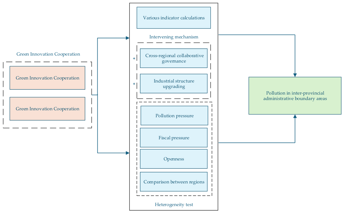
In order to more intuitively show the mechanism hypothesis of the paper, Figure 2 shows the mechanism analysis diagram between GIC and pollution control in provincial administrative boundary areas.

4. Empirical Model and Data

4.1. Baseline Model

To examine the impact of GIC on pollution in boundary areas, this paper specifies the following baseline regression model:
P o l l u t i o n i t = β 0 + β 1 G I C i t × B o r d e r i + β 2 X i t + C i t y i + Y e a r t + ε i t
where P o l l u t i o n i t is the dependent variable, measured by the logarithm of the annual average PM2.5 concentration in city i in year t . G I C i t × B o r d e r i is the core explanatory variable, representing the interaction between the number of intercity GICs and the inter-provincial boundary exposure intensity. X i t denotes a set of control variables, C i t y i represents city fixed effects, Y e a r t represents year fixed effects, and ε i t is the random error term.
To further examine the indirect mechanisms through which GIC affects pollution in boundary areas, this paper specifies the following mediation models:
M i t = γ 0 + γ 1 G I C i t × B o r d e r i + γ 2 X i t + C i t y i + Y e a r t + ε i t
P o l l u t i o n i t = φ 0 + φ 1 G I C i t × B o r d e r i + φ 2 M i t + φ 3 X i t + C i t y i + Y e a r t + ε i t
where M i t denotes the mechanism variable, including cross-regional collaborative governance and industrial structure upgrading. Equation (22) tests whether GIC affects the proposed mechanism variables, while Equation (23) examines whether these mechanisms further influence pollution levels after controlling for GIC and other covariates.

4.2. Variable Selection and Data Sources

4.2.1. Dependent Variable

This paper uses city-level annual average PM2.5 concentrations to measure pollution levels in inter-provincial boundary areas, mainly for the following reasons. First, PM2.5 is one of the most representative pollutants of urban air pollution and haze pollution in China. It reflects the combined effects of multiple pollution sources, including industrial combustion, energy consumption, traffic emissions, and secondary aerosol formation. Compared with single industrial pollutants, PM2.5 better captures residents’ actual exposure to air pollution and is also suitable for evaluating the overall effect of GIC on urban air quality improvement [66]. Second, PM2.5 has pronounced spatial diffusion and cross-regional transport characteristics. Pollutants do not remain strictly within administrative jurisdictions, but are affected by wind direction, topography, industrial layout, and energy consumption structure, generating spatial spillovers across neighboring cities. Therefore, for inter-provincial boundary cities, PM2.5 can better reflect pollution externalities and cross-boundary pollution governance pressure near administrative borders. Existing studies also show that PM2.5 pollution in Chinese cities exhibits significant spatial correlation and cross-city transmission effects, and that pollution conditions and environmental regulation in surrounding cities can affect local PM2.5 levels [67,68]. Third, compared with ground monitoring station data, satellite-derived PM2.5 data provide more complete spatial coverage and longer temporal continuity, which helps avoid sample bias caused by missing monitoring stations or inconsistent monitoring standards in some cities during earlier years. Specifically, this paper uses PM2.5 raster data for China from 2011 to 2023. The original global raster data are first clipped to the Chinese territory and then spatially matched with prefecture-level city administrative boundaries. The annual average PM2.5 concentration of each city is calculated based on all raster cells within its administrative boundary. The final city-level annual average PM2.5 indicator is measured in u g / m 3 . A higher value indicates more severe urban air pollution. The calculation formula is as follows:
P M 2.5 i , t = 1 N i g i P M 2.5 g , t
where P M 2.5 i , t denotes the annual average PM2.5 concentration of city i in year t , P M 2.5 i , t denotes the PM2.5 concentration of raster cell g within the administrative boundary of city i in year t , and N i is the number of raster cells included in the calculation for city i . To reduce the influence of right-skewness and extreme values on the estimation results, this variable is transformed using the natural logarithm in the empirical analysis and denoted as P o l l u t i o n .

4.2.2. Explanatory Variable

The explanatory variable is the interaction between green innovation collaboration ( G I C i t ) and inter-provincial boundary exposure intensity ( B o r d e r i ). Green innovation is often complex, systemic, and knowledge-complementary, so firms and regions may rely on external collaboration to obtain heterogeneous knowledge and compensate for weaknesses in their own green-technology capabilities [69]. Cross-regional innovation networks also facilitate knowledge diffusion and technological recombination and are important for green technological innovation [36]. We therefore measure GIC by the number of intercity green patent collaborations. When co-applicants for the same green patent are located in two or more prefecture-level cities, we identify the patent as an intercity GIC; joint applications among applicants within the same city are excluded. For patents involving multiple cities, collaborations are identified by each distinct city pair. We use two indicators: the number of intercity green-technology patent collaborations and the number of intercity green low-carbon patent collaborations. The former is identified from green-technology patent applications and grants from 2011 to 2023 by matching co-applicants’ coordinates and city affiliations; the latter is constructed analogously from green low-carbon patent applications and grants. If a green patent has co-applicants from different cities, it counts as one intercity GIC. Because these counts are strongly right-skewed and equal to zero for some city-years, we take ln(1 + x) for both measures and denote them by G T I and G L I . These count-based measures capture the frequency and breadth of intercity collaboration in a transparent way, with consistent statistical definitions and a clear economic interpretation. However, they assign the same technological value to different patent types and therefore do not fully capture differences in technological content and innovation quality. To incorporate quality, we construct quality-adjusted GIC measures by patent type. Invention patents generally face stricter examination, higher technological thresholds, and stronger originality than utility-model patents and therefore better capture substantive green innovation; utility-model patents more often reflect incremental, application-oriented improvements [45,70]. We assign weights of 0.7 to green-invention patents and 0.3 to green utility-model patents and construct quality-adjusted green-technology and green low-carbon collaboration measures in the same way, denoted by W G T I and W G L I . Design patents are excluded because they primarily concern product appearance rather than technical solutions and cannot be consistently identified as environmental technologies under an IPC-based green-technology classification.
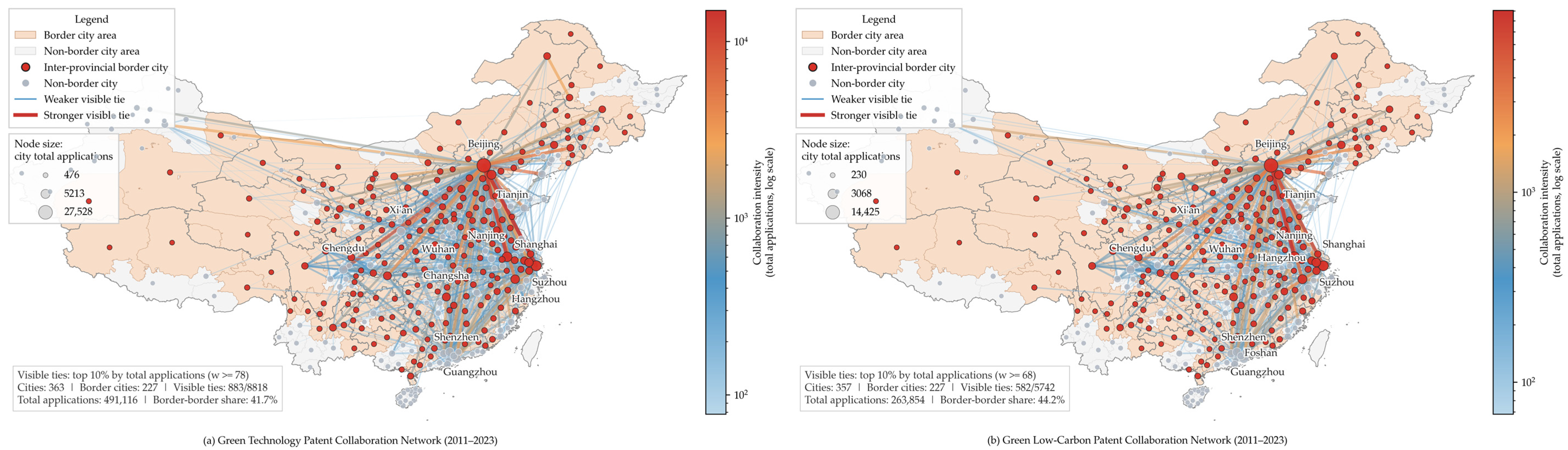
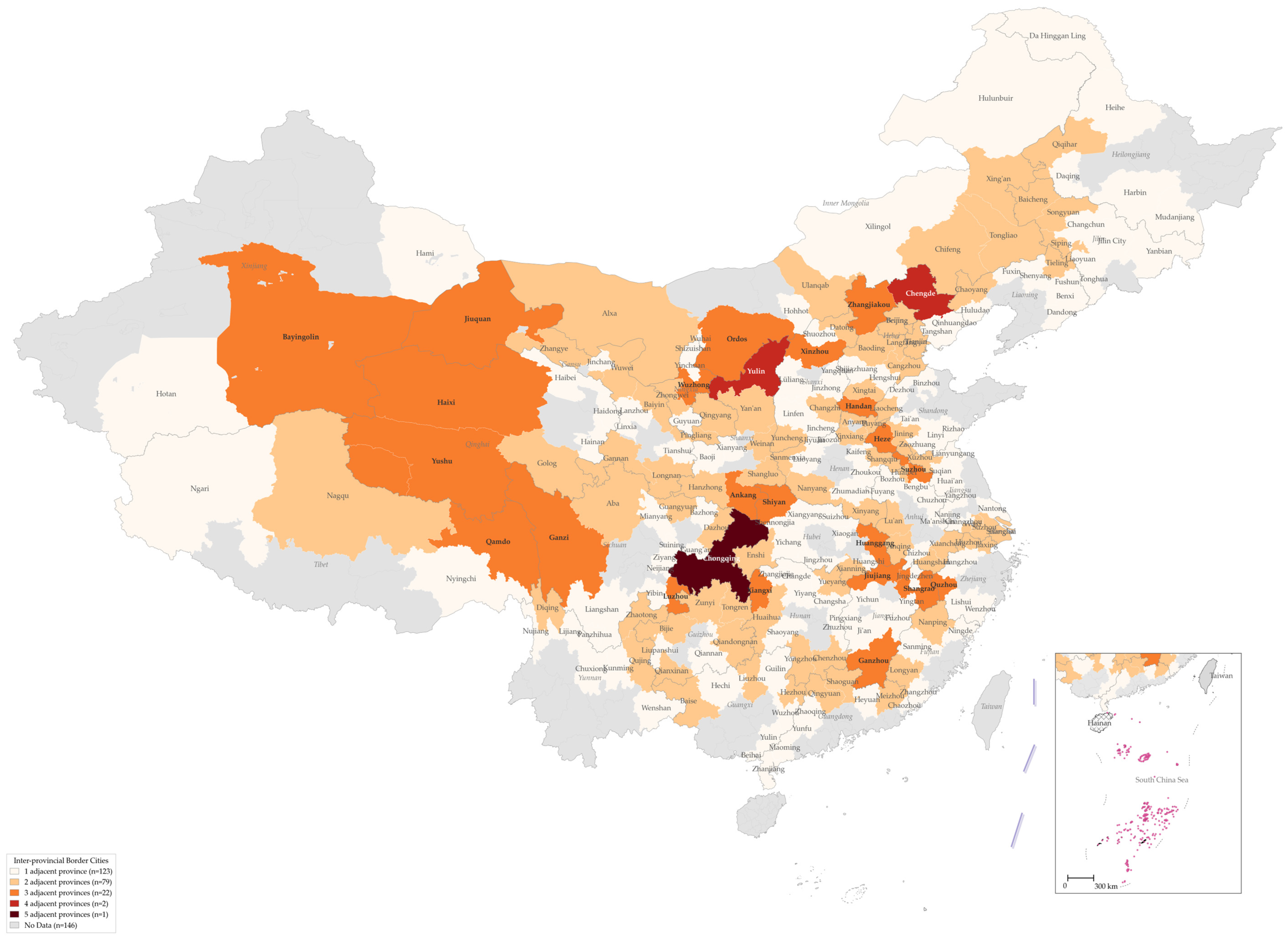
Figure 3 presents the green-technology patent collaboration network (a) and the green low-carbon patent collaboration network (b) among cities in inter-provincial boundary areas. The existence of these networks confirms that green patent collaboration occurs between cities; denser links indicate more active flows of green knowledge and joint R&D. GIC has therefore become an important channel through which inter-provincial boundary cities obtain external green knowledge, overcome administrative fragmentation, and improve pollution governance. To measure the degree of boundary contact across cities, we count the number of other provinces bordering each prefecture-level city and use it to map inter-provincial boundary cities in Figure 4. Darker colors indicate borders with more other provinces and therefore stronger boundary exposure; gray areas are non-boundary cities.
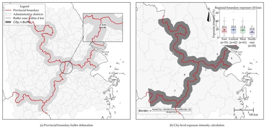
Evidence suggests that the boundary-pollution effect induced by environmental regulation is particularly pronounced within approximately 10 km of an administrative boundary [71]. After identifying inter-provincial boundary cities, we use GIS to overlay city administrative areas with a 10 km buffer around inter-provincial boundaries and calculate the share of each city’s area covered by the buffer. This creates a continuous index of inter-provincial boundary exposure intensity B o r d e r . The measure follows the boundary-effect literature, which uses administrative boundaries to identify institutional differences and spatial externalities [18,24,72]. It extends distance-based measures of boundary proximity to the city level, preserves the full sample, and captures differences in the relative exposure of cities to inter-provincial administrative boundaries. Compared with a simple boundary-city dummy, the exposure index more finely captures the share of a city located near an inter-provincial boundary and better matches the continuous spatial nature of transboundary pollution diffusion and boundary-governance pressure. The calculation is as follows:
B o r d e r i = A r e a C i t y i B u f f e r ( P r o v i n c i a l B o r d e r , d ) A r e a ( C i t y i )
where d denotes the buffer distance from the inter-provincial administrative boundary. Taking the inter-provincial boundary line as the reference line, this paper constructs buffer zones by extending d kilometers on both sides of the boundary line, as shown in Figure 5a, and calculates the ratio of the area of each city’s administrative territory falling within the buffer zone to the city’s total administrative area, as shown in Figure 5b. A larger value of this indicator indicates a higher degree of spatial exposure to inter-provincial administrative boundaries. This paper uses d = 10 km as the baseline measure and further adopts d = 20 km and d = 30 km buffer zones for robustness checks. In addition, non-boundary cities are assigned a value of zero rather than being directly excluded. This setting allows the full sample to be used in the regression analysis, enabling comparisons between boundary and non-boundary cities and providing a more comprehensive assessment of how the pollution governance effect of GIC varies with cities’ boundary attributes.

4.2.3. Control Variables

To mitigate potential omitted-variable bias, this paper controls for a set of socioeconomic factors that may affect urban PM2.5 concentrations. Existing studies show that urban air pollution is closely related not only to green technological innovation and environmental governance, but also to population agglomeration, economic development, industrial activity, openness, financial resource allocation, government intervention, and technological capacity [73]. Accordingly, the following control variables are included.
Population density ( D e n s i t y ) is measured by the ratio of a city’s permanent resident population to its administrative land area and is transformed using the natural logarithm. Higher population density may increase pollution emissions through transportation demand, residential energy consumption, and urban construction activities, but it may also improve energy-use efficiency through economies of scale and more compact public infrastructure.
Population mobility ( F l o w ) is measured by the ratio of the difference between permanent resident population and registered population to registered population. Population inflows may change urban energy consumption, transportation demand, and producer-service activities, while also affecting public service provision and environmental governance pressure, thereby influencing PM2.5 concentrations.
Economic development ( P g d p ) is measured by the logarithm of per capita regional GDP. Economic development may increase pollution through a larger production scale, energy consumption, and transportation activities, but it may also enhance cities’ capacity for environmental investment, clean technology adoption, and residents’ demand for environmental quality.
Openness ( O p e n ) is measured by the ratio of total imports and exports to regional GDP. Openness may increase pollution through industrial relocation and trade expansion, but it may also promote pollution reduction through technology spillovers, managerial knowledge transfer, and the improvement of environmental standards.
Human capital ( H u m a n ) is measured by the ratio of students enrolled in regular higher education institutions to total year-end population. A higher level of human capital strengthens a city’s ability to absorb, transform, and apply green technologies, and may also improve environmental governance efficiency and public environmental awareness.
Financial development ( F i n a n c e ) is measured by the ratio of outstanding loans of financial institutions to regional GDP. Financial development affects firms’ financing constraints and technological upgrading capacity, thereby influencing investment in clean production and pollution control.
Government intervention ( G o v ) is measured by the ratio of local general budgetary expenditure to regional GDP. The scale and intensity of fiscal intervention may affect urban infrastructure construction, environmental governance investment, and industrial resource allocation, and thus may influence PM2.5 concentrations.
Mobile phone penetration ( M o b i l e ) is measured by the ratio of year-end mobile phone users to registered population. Mobile communication infrastructure and information transmission capacity may affect access to environmental information, public supervision, and the level of digital environmental governance, thereby shaping pollution governance outcomes.
Science and technology level ( T e c h ) is measured by the ratio of science and technology expenditure to local general budgetary expenditure. Science and technology investment reflects a city’s innovation foundation and technological support capacity, which may affect green-technology R&D, the application of pollution control technologies, and environmental governance efficiency.

4.2.4. Data Sources

To ensure the reliability of the evaluation, cities with substantial missing values in key variables or obvious data abnormalities are excluded. The final research sample covers 293 Chinese cities over the period from 2011 to 2023. The choice of the period is motivated by China’s green and low-carbon policy trajectory. Beginning with the 12th Five-Year Plan, green development, energy conservation, emission reduction, and low-carbon transition became increasingly central to China’s development strategy. The launch of low-carbon city pilots in 2011—together with subsequent policies such as ecological civilization construction, air pollution prevention, carbon trading pilots, and the “dual carbon” targets—makes this period particularly suitable for examining the relationship between GIC and pollution governance. City-level annual average PM2.5 concentrations are obtained from the SatPM2.5 satellite-derived dataset released by the Atmospheric Composition Analysis Group at Washington University in St. Louis. This dataset integrates multi-source satellite aerosol optical depth, the GEOS-Chem chemical transport model, and ground-based monitoring observations, and therefore offers high spatial coverage and temporal continuity. Data on GIC are derived from green patent application and authorization records issued by the China National Intellectual Property Administration. The identification of interprovincial border cities is based on vector data on prefecture-level city administrative divisions and provincial administrative boundary data in China. All other municipal socio-economic data are derived from the China City Statistical Yearbook, the China City Construction Statistical Yearbook, the China Energy Statistical Yearbook, and City-level Statistical Bulletins on National Economic and Social Development from each year. The descriptive statistics for all aforementioned variables are systematically reported in Table 1.

5. Empirical Results

5.1. Baseline Regression

Table 2 reports the baseline estimates of the effect of GIC on pollution in inter-provincial boundary cities. Columns (1)–(4) use count-based collaboration measures, while columns (5)–(8) use quality-adjusted measures that distinguish the technological value of invention and utility-model patents. The coefficients on the interaction between GIC and boundary exposure intensity are negative and statistically significant in all specifications, indicating that GIC significantly reduces PM2.5 in cities with greater exposure to inter-provincial boundaries. Without controls, the coefficient is G T I × b o r d e r −0.0565 and significant at the 1% level in column (1) and G L I × b o r d e r −0.0459 and significant at the 5% level in column (2). After adding controls, the coefficient on G T I × b o r d e r in Column (3) remains −0.0369 and is statistically significant at the 5% level. Its economic implication is that, when boundary exposure intensity equals 1, a one-unit increase in the log-transformed count-based measure of green-technology patent collaboration is associated with an approximately 3.62% decrease in a city’s annual average PM2.5 concentration. In Column (4), the coefficient on G L I × b o r d e r is −0.0312 and is statistically significant at the 10% level. This implies that, when boundary exposure intensity equals 1, a one-unit increase in the log-transformed count-based measure of green low-carbon patent collaboration is associated with an approximately 3.07% decrease in a city’s annual average PM2.5 concentration. Columns (5)–(8) report estimates using quality-adjusted measures. Without controls, the coefficients are W G T I × b o r d e r −0.0591 and W G L I × b o r d e r −0.0486 and are significant at the 1% and 5% levels in columns (5) and (6), respectively. With controls, the coefficient on W G T I × b o r d e r in Column (7) is −0.0378 and is statistically significant at the 5% level. Its economic implication is that, when boundary exposure intensity equals 1, a one-unit increase in the log-transformed quality-adjusted measure of green-technology patent collaboration is associated with an approximately 3.71% decrease in a city’s annual average PM2.5 concentration. In Column (8), the coefficient on W G L I × b o r d e r is −0.0319 and is statistically significant at the 10% level. This implies that, when boundary exposure intensity equals 1, a one-unit increase in the log-transformed quality-adjusted measure of green low-carbon patent collaboration is associated with an approximately 3.14% decrease in a city’s annual average PM2.5 concentration. The two sets of measures yield similar signs, magnitudes, and significance levels. The baseline conclusion therefore survives adjustment for differences in patent quality and is not driven by assigning the same technological value to different patent types.
These estimates show that, after controlling for city fixed effects, year fixed effects, and a range of socioeconomic factors, both green-technology and green low-carbon patent collaboration significantly improve pollution conditions in inter-provincial boundary areas. This finding is consistent with Zhao et al. (2023) [47], who show that collaborative green innovation can generate stronger carbon-reduction effects. Our study further shows that collaborative green innovation continues to reduce pollution in inter-provincial boundary areas, where transboundary pollution diffusion and administrative fragmentation coexist. This effect arises because joint R&D and patent collaboration connect technical knowledge dispersed across cities with local application needs, thereby reducing the cost of accessing and adopting green technologies in boundary areas. Boundary cities can consequently obtain clean-production and pollution-control technologies suited to their local industries at lower cost, while collaborative networks facilitate the diffusion of these technologies among boundary cities. The unchanged results under quality-adjusted measures indicate that the estimates are not primarily driven by the accumulation of low-technology-content patents. Because the subsequent mechanism, heterogeneity, and spatial analyses focus mainly on the frequency of intercity collaboration, its transmission channels, and spatial diffusion, the count-based measures are more transparent economically and more comparable across models. After confirming that the baseline conclusion is not sensitive to differences in patent quality, we therefore use the count-based G T I and G L I measures in the subsequent analyses.

5.2. Robustness Checks

5.2.1. Alternative Measures of the Explanatory Variables

First, we replace the measure of inter-provincial boundary exposure intensity. In the baseline regressions, it is the share of each city’s area falling within a 10 km buffer of an inter-provincial boundary. To ensure that the estimates are not driven by the buffer distance, we expand the distance to 20 km and 30 km and reconstruct the exposure index. Columns (1)–(4) in Table 3 show that the interaction terms remain significantly negative when 20 km and 30 km buffers are used. We also replace the boundary measure with a 0/1 dummy that equals one for inter-provincial boundary cities and zero otherwise. Columns (5) and (6) show that the core explanatory variable remains significantly negative. Finally, we divide green-technology and green low-carbon collaboration patents into invention and utility-model patents and interact each of the four measures with boundary exposure intensity. Columns (7)–(10) show significantly negative coefficients for all four alternative collaboration measures, indicating that GIC reduces pollution in inter-provincial boundary areas whether it is measured by invention or utility-model patents.

5.2.2. Alternative Measures of the Dependent Variable

This paper further replaces the pollution measure. First, considering that urban air pollution may be affected not only by local emissions but also by province-level common shocks and regional background pollution, this paper uses the difference between the logarithm of city-level annual average PM2.5 concentration and the logarithm of the corresponding provincial annual average PM2.5 concentration as an alternative dependent variable. This measure captures the pollution gap of a city relative to the provincial average. The results in columns (1) and (2) of Table 4 show that the coefficients of the core explanatory variables remain significantly negative, indicating that GIC reduces the relative pollution level of inter-provincial boundary cities.
Second, this paper directly uses the level value of city-level annual average PM2.5 concentration as the dependent variable, replacing the logarithmic PM2.5 measure used in the baseline regression. Columns (3) and (4) of Table 4 show that the interaction terms between green-technology innovation collaboration, green low-carbon innovation collaboration, and boundary exposure intensity remain significantly negative. This suggests that the main conclusion is not driven by the logarithmic transformation of PM2.5.
Third, this paper further uses the logarithm of city-level annual average SO2 concentration as an alternative pollution indicator. SO2 is an important pollutant generated from energy combustion and industrial emissions, and is closely associated with fossil fuel consumption and industrial production activities. The results in columns (5) and (6) of Table 4 show that GIC also has a significant inhibitory effect on SO2 pollution. This indicates that GIC not only improves PM2.5 pollution but also contributes to the reduction of other air pollutants.

5.2.3. Excluding Potential Policy Confounders

This paper further considers whether contemporaneous environmental policies may interfere with the estimated results and conducts exclusion tests accordingly. First, since 2014, the Yangtze River Delta has continuously promoted regional cooperation in air pollution prevention and control. Such joint prevention and control policies may directly improve air quality and thus confound the estimated effect in this paper. To address this concern, this paper re-estimates the model after excluding the samples from the three provinces and one municipality in the Yangtze River Delta. The results in columns (7) and (8) of Table 4 show that, after excluding the Yangtze River Delta sample, the coefficients of the core explanatory variables remain significantly negative. This indicates that the main conclusion is not driven by regional collaborative air pollution control policies in the Yangtze River Delta.
Second, between 2007 and 2014, the central government successively approved 12 regions, including Jiangsu, Tianjin, and Zhejiang, as pilot areas for SO2 emissions trading. This policy may directly affect urban air quality through emissions permit constraints and pollution-control incentives, thereby interfering with the estimated effect of GIC. Therefore, this paper controls for the SO2 emissions trading pilot policy in the regression. The results in columns (9) and (10) of Table 4 show that, after controlling for this policy, the interaction terms between green-technology innovation collaboration, green low-carbon innovation collaboration, and boundary exposure intensity remain significantly negative.
Third, the Air Pollution Prevention and Control Action Plan, issued by the State Council in 2013, was a major policy initiative in China’s air pollution governance. The policy may have affected urban air quality, industrial restructuring, and investment in pollution governance. Because it constituted a nationwide policy shock, its post-implementation dummy variable would be absorbed by the year fixed effects if entered separately. This study therefore constructs an interaction between the post-policy dummy variable and interprovincial boundary exposure intensity and includes it in the baseline model. The model is specified as follows:
P o l l u t i o n i t = β 0 + β 1 G I C i t × B o r d e r i + γ 1 P o s t A i r t × B o r d e r i + β 2 X i t + C i t y i + Y e a r t + ε i t
where P o s t A i r t is a post-policy dummy variable for the Air Pollution Prevention and Control Action Plan. It equals 1 in 2013 and subsequent years and 0 otherwise. The interaction P o s t A i r t × B o r d e r i controls for the possibility that this nationwide air pollution policy had differential effects on cities with different levels of interprovincial boundary exposure. As reported in Columns (1) and (2) of Table 5, the coefficients of the core explanatory variables are −0.0305 and −0.0273, respectively, and both are significantly negative at the 10% level. Thus, after accounting for the interaction between the national air pollution policy and boundary exposure intensity, GIC continues to reduce pollution in interprovincial boundary areas. The baseline findings are therefore not driven by the Air Pollution Prevention and Control Action Plan.
Fourth, in 2011, the National Development and Reform Commission approved carbon emissions trading pilots in Beijing, Tianjin, Shanghai, Chongqing, Hubei, Guangdong, and Shenzhen. This policy may affect urban pollution emissions by imposing carbon-reduction constraints, encouraging green technological innovation, and promoting low-carbon industrial transformation. Given the marked regional variation in the carbon trading pilot policy, this study constructs an interaction between the pilot-region dummy variable and the post-policy dummy variable. This treatment term is further interacted with interprovincial boundary exposure intensity to control for the potential effect of the carbon trading pilots on pollution governance in boundary areas. The model is specified as follows:
P o l l u t i o n i t = β 0 + β 1 G I C i t × B o r d e r i + γ 2 E T S i × P o s t E T S t + γ 3 E T S i × P o s t E T S t × B o r d e r i + β 2 X i t + C i t y i + Y e a r t + ε i t
where E T S i is a dummy variable for the carbon emissions trading pilot regions. It equals 1 for cities in Beijing, Tianjin, Shanghai, Chongqing, Hubei, Guangdong, and Shenzhen and 0 otherwise. P o s t E T S t is a post-policy dummy variable for the implementation of the carbon trading pilot. The term E T S i × P o s t E T S t captures the average effect of the pilot policy, while E T S i × P o s t E T S t × B o r d e r i controls for its differential effect on pollution governance in interprovincial boundary areas. As shown in Columns (3) and (4) of Table 5, after controlling for the carbon emissions trading pilot, the coefficients of the core explanatory variables are −0.0316 and −0.0268, respectively, and both remain significantly negative at the 10% level. These findings indicate that the carbon trading pilots do not account for the pollution-reduction effect of GIC in interprovincial boundary areas, further supporting the robustness of the baseline results.

5.2.4. Annual 1% and 5% Winsorization

To mitigate the influence of extreme values on the estimation results, the dependent variable, core explanatory variables, and control variables are winsorized at both tails by year at the 1% and 5% levels. This treatment reduces the influence of anomalous observations while preserving the relative distribution of the variables within each year. As shown in Columns (5)–(8) of Table 5, the coefficients of the core explanatory variables remain significantly negative after both the 1% and 5% winsorization procedures, consistent with the baseline estimates. These results indicate that the findings are not driven by a small number of extreme observations and confirm the robustness of the pollution-reduction effect of GIC in interprovincial boundary areas.

5.2.5. Inclusion of Prefecture-Level Nighttime Light Data

To reduce potential measurement bias associated with conventional indicators of economic scale, this study further incorporates prefecture-level nighttime light data as a robustness check. The data are obtained from the NPP–VIIRS nighttime light remote-sensing dataset, which is generated by satellite observation systems operated by NASA and NOAA and provides a useful measure of human activity and urban economic intensity on the Earth’s surface. Annual mean nighttime light intensity is used as the prefecture-level nighttime light indicator and is included in the baseline regression model. As reported in Columns (9) and (10) of Table 5, the signs and statistical significance of the core coefficients remain consistent with the baseline results after nighttime light data are included.

5.2.6. Endogeneity Tests

The relationship between GIC and boundary pollution governance may remain subject to endogeneity. First, cities with more severe pollution may be more inclined to engage in GIC, creating a potential reverse-causality problem. Second, unobserved factors—such as urban governance capacity, the innovation environment, and regional policies—may simultaneously affect GIC and pollution governance performance, thereby generating omitted-variable bias. In addition, interprovincial boundary cities are geographically connected and subject to transboundary pollution transmission. Pollutant diffusion, green-technology cooperation, and governance behavior may therefore exhibit spatial dependence. If these spatial interactions are ignored, the baseline estimates may be biased by omitted spatially lagged terms. To mitigate these concerns, this study conducts three complementary analyses. First, an instrumental variable approach is employed to address potential reverse causality and omitted-variable bias. Second, because participation in GIC is not randomly distributed across cities, a Heckman two-stage model is used to correct for potential sample-selection bias. Third, a spatial Durbin model is constructed that incorporates spatial lags of both the dependent variable and the core explanatory variables. This model is used to estimate the direct effects and spatial spillover effects of GIC on pollution governance in interprovincial boundary areas.
(1) Instrumental Variable Approach. This paper first constructs instrumental variables for the number of intercity green-technology innovation collaborations and green low-carbon innovation collaborations. Specifically, the two collaboration variables are lagged by one period, their annual city-level means are calculated, and then they are interacted with inter-provincial boundary exposure intensity to construct the instrumental variables I V 1 and I V 2 . In terms of relevance, green innovation collaboration exhibits strong path dependence and network persistence, so the one-period lagged level of urban green innovation collaboration can predict current green innovation collaboration reasonably well. With respect to the exogeneity rationale, the one-period lagged average of collaboration is less directly correlated with contemporaneous pollution shocks, which helps reduce the possibility that the instrument changes simultaneously with current pollution while retaining predictive power for current green innovation collaboration (to examine the exclusion restriction of the one-period-lagged instrumental variable, we include IV2 in the model and use the two-period-lagged instrumental variable, IV4, to identify current green low-carbon innovation collaboration. The second-stage results show that the coefficient on IV2 is 2.1803 and is not statistically significant at the 10% level. This indicates that, after controlling for current green low-carbon innovation collaboration identified through the instrumental variable approach, we find no evidence of an additional direct effect of IV2 on current PM2.5, thereby providing support for the exclusion restriction of IV2. The same reasoning applies to IV1; the details are therefore not repeated.). Table 6 reports the estimation results of the instrumental variable approach. The first-stage results show that the coefficients of I V 1 and I V 2 are 0.5723 and 0.4715, respectively, and both are significant at the 1% level, indicating a strong correlation between the instruments and the endogenous explanatory variables. The KP rk LM statistics are 53.176 and 51.869, respectively, both significant at the 1% level, rejecting the null hypothesis of underidentification. The KP rk Wald F statistics are 451.232 and 233.985, respectively—both are substantially larger than conventional critical values, suggesting that weak-instrument concerns are unlikely to materially affect the estimates. The second-stage results show that the coefficients of G T I × b o r d e r and G L I × b o r d e r are −6.1486 and −6.6509, respectively, and both are significant at the 1% level. These results suggest that—conditional on the validity of the exclusion restriction—green-technology and green low-carbon innovation collaboration remain negatively associated with pollution levels in inter-provincial administrative boundary areas when their lagged mean levels are used as instrumental variables, providing additional support for the robustness of the baseline findings.
To provide further evidence regarding the exclusion restriction of the instrumental variables, this study uses the interactions between two-period lagged patent cooperation and interprovincial boundary exposure intensity as alternative instruments. Specifically, I V 3 is constructed as the interaction between two-period lagged green-technology patent cooperation and boundary exposure intensity, while I V 4 is constructed as the interaction between two-period lagged green low-carbon patent cooperation and boundary exposure intensity. It should be noted that using a two-period lag can reduce the likelihood that the instrument is affected by contemporaneous pollution shocks, but it cannot fully rule out the possibility that historical collaboration directly affects current pollution through persistent knowledge networks, industrial pathways, or policy continuity. Therefore, this test provides supplementary evidence consistent with the exclusion restriction rather than directly validating it. The results are reported in Columns (5)–(8) of Table 6. The first-stage estimates show that I V 3 and I V 4 are significantly and positively associated with their corresponding endogenous variables. Their coefficients are 0.4470 and 0.3455, respectively, and both are significant at the 1% level. The KP rk LM statistics are 47.289 and 51.589, respectively, rejecting the null hypothesis of underidentification. Moreover, the KP rk Wald F statistics are 199.698 and 120.037, both substantially above the conventional critical values, indicating that weak-instrument concerns are unlikely to affect the estimates. In the second-stage regressions, the coefficients of G T I × b o r d e r and G L I × b o r d e r remain significantly negative at −9.0541 and −10.1364, respectively. Conditional on the validity of the exclusion restriction, these results suggest that the estimated pollution-governance effect of GIC in inter-provincial administrative boundary areas remains statistically significant when the two-period lagged instruments are used.
(2) Heckman Two-Stage Method. GIC does not occur uniformly across all cities. Some cities may not participate in GIC for a long time due to weak historical innovation foundations, a lack of collaboration networks, or insufficient innovation resources. Estimating the effect only among cities with observed collaboration may therefore lead to sample selection bias. To address this issue, this paper further applies the Heckman two-stage method. Specifically, the number of intercity patent collaborations during 1985–2010 is used to construct the historical innovation collaboration network ( H i s t o r y C o o p i ) as an explanatory variable in the first-stage selection equation. The dependent variables are whether a city engages in green-technology innovation collaboration ( C o o p _ G ) and green low-carbon innovation collaboration ( C o o p _ L ), which equal 1 if collaboration occurs and 0 otherwise. The historical collaboration network captures a city’s pre-existing collaboration foundation and network embeddedness before the formation of GIC and is expected to have strong explanatory power for subsequent participation in GIC. Meanwhile, since this variable is formed before the sample period, it is less likely to be affected by pollution governance shocks during 2011–2023. In the first stage, this paper estimates the probability that a city participates in green-technology innovation collaboration and green low-carbon innovation collaboration, respectively, and calculates the inverse Mills ratio ( I M R ). In the second stage, the I M R is included in the baseline regression model to correct for potential sample selection bias. Table 7 reports the Heckman two-stage estimation results. The first-stage results show that H i s t o r y C o o p has a significantly positive effect on the probability of participating in both green-technology innovation collaboration and green low-carbon innovation collaboration, with coefficients of 0.3841 and 0.4354, respectively, both significant at the 1% level. This indicates that the historical innovation collaboration network can effectively explain cities’ subsequent participation in GIC. The second-stage results show that, after controlling for I M R , the coefficients of G T I × b o r d e r and G L I × b o r d e r are −0.0312 and −0.0447, respectively, and are significant at the 10% and 5% levels. This suggests that, after correcting for sample selection bias, the pollution governance effect of GIC in inter-provincial boundary areas remains valid. In addition, the coefficient of I M R is significant, indicating that sample selection bias does exist and that applying the Heckman two-stage method is necessary.
(3) Spatial Durbin Model. To account for the spatial dependence of urban pollution and the spatial spillovers of GIC, this study further constructs the following spatial Durbin model:
P o l l u t i o n i t = ρ j = 1 N w i j P o l l u t i o n j t + β 1 G I C i t × B o r d e r i + θ 1 j = 1 N w i j G I C j t × B o r d e r j + β 2 X i t + θ 2 j = 1 N w i j X j t + C i t y i + Y e a r t + ε i t
where W = ( w i j ) denotes the spatial weight matrix. This study employs a row-standardized city contiguity matrix. If cities i and j are adjacent, w i j > 0 ; otherwise, w i j = 0 . After row standardization, the matrix satisfies j = 1 N w i j = 1 . The parameter ρ is the spatial autoregressive coefficient and captures the effect of pollution in neighboring cities on local pollution. The coefficient θ 1 measures the spatial spillover effect of GIC in neighboring cities on local pollution governance, while θ 2 captures the spatial effects of neighboring cities’ socioeconomic characteristics on local pollution.
Table 8 reports the global Moran’s I statistics for urban PM2. concentrations from 2011 to 2023. Moran’s (I) is positive throughout the sample period, ranging from 0.3914 to 0.5252. The corresponding (z)-statistics all exceed 10, with (p)-values of 0.0005, indicating significant positive spatial dependence in urban PM2. concentrations. In other words, PM2.5 is not randomly distributed across cities but exhibits pronounced spatial clustering: high-pollution cities tend to be surrounded by other high-pollution cities, while low-pollution cities are more likely to be located near other low-pollution cities. These findings confirm that air pollution has significant spatial spillovers and regional linkages. Consequently, conventional two-way fixed-effects models may produce biased estimates if spatial interactions are ignored. The spatial Durbin model therefore incorporates spatial lags of both the dependent and explanatory variables to test the robustness of the estimated effect of GIC on pollution governance in interprovincial boundary areas.
Table 9 reports the spatial Durbin estimates. City-level PM2.5 pollution displays significant spatial dependence, consistent with the Moran’s I results. After controlling for spatial lags of both the dependent and explanatory variables, the direct effect of the interaction between green-technology innovation collaboration and inter-provincial boundary exposure intensity is significantly negative. The direct effect of the corresponding interaction for green low-carbon innovation collaboration is also significantly negative, indicating that GIC significantly reduces local PM2.5 pollution in inter-provincial boundary cities. This finding is consistent with Zhao et al. (2023) [47], who show that collaborative green innovation can reduce carbon emissions, but it extends the environmental effect to air-pollution governance in inter-provincial boundary cities and indicates that the environmental gains from intercity green-technology collaboration are not limited to carbon reduction. The indirect effect of the core explanatory variable is also significantly negative. Ge et al. (2023) argue that regional collaborative governance can reduce urban air pollution and generate pollution-reduction effects within a certain spatial range, which is consistent with our estimates [29]. Green knowledge entering neighboring cities through collaboration networks can lower the search, matching, and application costs of clean technologies, thereby encouraging surrounding cities to improve production processes and pollution-control technologies and reduce emissions. Thus, after controlling for spatial dependence in urban pollution and the spatial spillovers of GIC, the baseline conclusion remains supported.

5.3. Heterogeneity Analysis

To further examine whether the effect of GIC on pollution governance in interprovincial boundary areas varies across urban contexts, and to address the inability of subsample regressions to formally test the statistical significance of between-group differences, this study employs a triple-interaction model. Specifically, cities are differentiated according to pollution pressure, fiscal pressure, and the level of openness. For each dimension, a high-group dummy variable, H i g h i t , is constructed. The following model is then estimated:
P o l l u t i o n i t = α 0 + α 1 G I C i t × B o r d e r i + α 2 G I C i t × B o r d e r i × H i g h i t + β X i t + C i t y i + Y e a r t + ε i t
In this specification, α 2 captures the difference in the effect of GIC between the high and low groups, while ( α 1 + α 2 ) represents the total effect for cities in the high group. All other parameters are defined as in the preceding models. A linear combination test is subsequently used to estimate and assess the statistical significance of the total effect in the high group. This approach makes it possible to formally determine whether the pollution governance effect of GIC differs significantly across urban contexts.

5.3.1. Pollution Pressure

We divide cities into high- and low-pollution-control-pressure groups using the median of annual average city-level PM2.5 concentrations. Columns (1) and (2) of Table 10 report the triple-interaction results. In the low-pressure group, the core effects of green-technology and green low-carbon innovation collaboration are 0.0204 and 0.0232, respectively, and neither is statistically significant. The effect of GIC on boundary-pollution governance is therefore not evident in cities facing relatively low pollution pressure. The coefficients on the interactions between the core explanatory variables and the high-pressure indicator are −0.0897 and −0.0860, respectively—both significant at the 1% level, showing that pollution-control pressure significantly strengthens the pollution-governance effect of GIC. Linear-combination tests show that the total effects in the high-pressure group are −0.0692 and −0.0628, both significant at the 1% level. The pollution-reduction effect of GIC is therefore concentrated in cities facing greater pollution-control pressure. This finding is directionally consistent with Cheng et al. (2023) [74], who show that stringent emission-reduction targets increase firms’ green-invention applications. Our study shifts the focus from green innovation output to pollution-governance performance. When pollution pressure is high, technologies generated through intercity collaboration are more likely to be adopted by local governments and firms. High-pollution boundary cities face more urgent air-quality objectives, while firms face greater compliance costs and reputational losses; collaborative clean-production and monitoring technologies can consequently enter production and governance more quickly. Low-pressure cities lack the same governance demand, and the fixed cost of adopting new technologies may not be covered by short-term emission-reduction benefits, so collaboration does not generate a significant pollution-reduction effect.

5.3.2. Fiscal Pressure

Fiscal pressure affects local governments’ ability to promote green-technology application, implement pollution-governance projects, and support cross-regional collaboration. We divide the sample into high- and low-fiscal-pressure groups at the median. Columns (3) and (4) of Table 10 show that in the low-pressure group, the core effects of green-technology and green low-carbon innovation collaboration are −0.0720 and −0.0618, respectively—both significantly negative. GIC therefore significantly reduces pollution in inter-provincial boundary areas when fiscal pressure is relatively low. The coefficients on the interactions between the core explanatory variables and the high-fiscal-pressure indicator are 0.0544 and 0.0481, respectively—both significant at the 10% level, indicating that fiscal pressure weakens the pollution-governance effect. The total effects in the high-pressure group are −0.0176 and −0.0137—neither statistically significant. The emission-reduction effect of GIC thus appears mainly in cities with lower fiscal pressure. This result is consistent with Peng et al. (2023) [75], who found that fiscal tightening can lead local governments to relax environmental regulation and increase firms’ pollution emissions. Their study emphasizes the effect of fiscal pressure on regulatory behavior; our results further indicate that fiscal pressure determines whether the outcomes of green collaboration can be implemented. When fiscal pressure is low, local governments can bear up-front costs and use project arrangements and environmental regulation to encourage firms to adopt new technologies. When fiscal pressure is high, basic public expenditure and stable tax revenue take priority, squeezing investment in green-technology commercialization and joint governance, so the collaboration effect becomes insignificant.

5.3.3. Openness

Openness affects a city’s ability to obtain external knowledge, technologies, and management experience and may also shape the efficiency with which GIC is absorbed and commercialized. We divide cities into high- and low-openness groups at the median. Columns (5) and (6) of Table 10 show that in the low-openness group, the core effects of green-technology and green low-carbon innovation collaboration are −0.0199 and −0.0140, respectively—neither statistically significant. The pollution-governance effect is therefore not evident in cities with low openness. The coefficients on the interactions between the core explanatory variables and the high-openness indicator are −0.0587 and −0.0514, respectively—both significant at the 10% level, showing that openness strengthens the pollution-governance effect. The total effects in the high-openness group are −0.0786 and −0.0654 and are significant at the 1% and 5% levels, respectively. Higher openness therefore makes it more likely that GIC will translate into observable emission reductions. Li et al. (2021) argue that greater openness attracts more foreign direct investment and promotes green innovation output through technology spillovers [57]. Our results further show that openness affects the efficiency with which collaborative technologies move from R&D to application. More open cities have better access to external suppliers and specialized technical-service providers, which can provide equipment, performance testing, and market validation for collaborative patents and thus lower technology-adaptation costs. Cities with low openness lack these complementary conditions, so knowledge created through intercity collaboration is less likely to enter local production and pollution governance, and its emission-reduction effect is not significant.

5.3.4. Regional Heterogeneity

The descriptive patterns in Figure 1 suggest that regional differences in green innovation foundations, absorptive capacity, fiscal constraints, and openness may shape the pollution-governance effect of GIC. We therefore examine the heterogeneous effects of pollution pressure, fiscal pressure, and openness separately in the eastern, central, western, and northeastern regions; the results are reported in Table 10. The eastern results are relatively stable. For pollution pressure, the coefficients of GTI and GLI in the low-pressure group are −0.0576 and −0.0593, respectively—both significant at the 1% level; the total effects in the high-pressure group are −0.0349 and −0.0353 and remain significantly negative. The difference between the high- and low-pressure groups is not significant, indicating that GIC has a relatively broad emission-reduction effect in eastern cities, but its intensity does not change significantly with pollution pressure. For fiscal pressure, the total effects are significantly negative in both the low- and high-pressure groups, and the between-group difference is not significant. This suggests that the eastern region’s more developed innovation system and technology commercialization conditions partly reduce the constraints imposed by fiscal pressure on green-technology application. For openness, the total effects of GTI and GLI in the high-openness group are −0.0504 and −0.0514, respectively—both significant at the 1% level. Although the difference between groups is not significant, GIC still has a stable pollution-reduction effect in eastern cities with relatively high openness. This is consistent with the clear downward trend in PM2.5 concentrations among eastern border cities shown in Figure 1. The effect is weaker in the central region. For pollution pressure and openness, the low-group effects, the high–low differences, and most high-group total effects are not significant, indicating that GIC has not yet been translated consistently into pollution-governance performance. For fiscal pressure, the total effect of GTI is significantly positive in the high-pressure group, while the corresponding GLI estimate is not significant. Fiscal constraints may therefore affect the conversion of green R&D outcomes into operational governance capacity, but the pattern is not consistent across green innovation measures. Although Figure 1 shows a clear decline in PM2.5 concentrations in central border cities, the estimates in Table 10 suggest that the decline may also reflect environmental regulation, industrial restructuring, and pollution-control investment rather than GIC alone. The western region displays greater consistency. Under different pollution- and fiscal-pressure conditions, the total effects of GTI and GLI are mostly negative, indicating an overall pollution-reduction effect, although most high–low differences are not significant. For openness, the low-group coefficients of GTI and GLI are −0.0323 and −0.0266, respectively, while the total effects in the high-openness group increase in absolute value to −0.0488 and −0.0664. The interaction between GLI and the high-openness indicator is significantly negative, showing that greater openness significantly strengthens the emission-reduction effect of green low-carbon innovation collaboration. Openness may expand sources of clean technology, improve cross-regional knowledge flows, and enhance green-technology absorptive capacity, thereby helping collaborative outcomes translate into pollution-governance performance. This result is broadly consistent with the steady decline in pollution among western border cities shown in Figure 1. The northeastern region exhibits stronger conditional dependence and greater temporal volatility. Under the pollution-pressure dimension, the total effects of GTI and GLI in the high-pressure group are significantly negative. Figure 1 shows particularly pronounced fluctuations in PM2.5 among northeastern border cities: concentrations rose rapidly during 2013–2015, declined markedly during 2016–2018, rebounded temporarily during 2019–2020, and then declined again before increasing slightly in 2023. Because the northeastern subsample is relatively small ( n = 20 ), large fluctuations in pollution may magnify the group estimates. Under the fiscal-pressure dimension, the core effects of GTI and GLI in the low-pressure group are −0.0131 and −0.0148, respectively—both significant at the 1% level. The interaction terms in the high-pressure group are 0.0351 and 0.0378, making the total effects 0.0220 and 0.0230; all are significant at the 1% level. Greater fiscal pressure may therefore weaken or even reverse the environmental-improvement effect of GIC. Under the openness dimension, the core effect in the low-openness group is significantly negative, whereas the total effect in the high-openness group remains negative but is no longer significant, indicating that its emission-reduction effect has not yet formed a stable pattern.

5.4. Mechanism Analysis

The baseline regression results show that GIC significantly reduces pollution in interprovincial boundary areas. To identify the channels underlying this effect, this study examines two mechanisms: cross-regional collaborative governance and industrial structure upgrading. Specifically, these two indicators are introduced as mechanism variables to assess whether GIC improves pollution governance in interprovincial boundary areas by strengthening governance coordination across jurisdictions and promoting the transition of industrial activity toward technology-intensive, higher-value-added, and less-polluting sectors.
Cross-regional collaborative governance (COG): This paper constructs an indicator of cross-regional collaborative governance using the “Prefecture-Level Cities: Collaborative Development and Environmental Co-Governance” text dataset from the Government Environmental Attention Database (GEAD). The database uses local government work reports as its textual source and records keyword frequencies related to collaborative development and environmental co-governance, excluding English words and numerical characters. Because pollution governance in interprovincial boundary areas emphasizes cross-regional joint prevention and control, collaborative pollution abatement, and joint governance, this study selects the keywords “environmental coordination,” “joint prevention,” “joint control,” “joint governance,” “conservation cooperation,” “collaborative pollution abatement,” and “collaborative governance.” The total annual frequency of these terms within each city is used to measure the local government’s policy attention to cross-regional collaborative governance. The indicator is constructed as follows.
First, the frequencies of the selected keywords in city i and year t are summed to obtain the total frequency of cross-regional collaborative governance terms:
C O G _ c o u n t i t = k K W F r e C y _ C o u n t i t k
where W F r e C y _ C o u n t denotes the frequency of keyword K in the government work report of city ( i ) in year ( t ), and ( K ) denotes the set of cross-regional collaborative governance keywords selected in this study.
To account for differences in the length of local government work reports, the keyword count is standardized by the total number of words in each report, denoted by W o r d _ O n l y , and converted into occurrences per 10,000 words:
C O G _ p e r 10 k i t = C O G _ c o u n t i t W o r d _ O n l y i t × 10,000
Finally, because the indicator is right-skewed and the keyword frequency is zero for some city-year observations, a natural logarithmic transformation after adding one is applied:
C O G i t = ln 1 + C O G _ p e r 10 k i t
A larger value of this indicator indicates that the local government devotes greater attention in its work report to cross-regional coordination, joint prevention and control, and collaborative governance, and therefore exhibits a stronger policy orientation toward cross-regional collaborative governance.
Industrial structure upgrading (ISU): This study measures industrial structure upgrading using the spatial vector angle method. This approach represents the three-sector industrial structure as a spatial vector and calculates the angles between the observed industrial structure vector and a set of standard vectors representing the progression from lower- to higher-level industries. These angles capture the extent to which the industrial structure shifts from the primary sector to the secondary and tertiary sectors. Compared with measures based solely on the share of the tertiary sector or the ratio of the tertiary sector to the secondary sector, the spatial vector angle method captures relative structural changes across all three sectors and reduces the limitations associated with a single indicator. The measure is constructed as follows.
Let s 1 i t , s 2 i t , and s 3 i t denote the shares of the value added of the primary, secondary, and tertiary sectors, respectively, in the GDP of city i in year t . The observed industrial structure vector is defined as
V i t = s 1 i t , s 2 i t , s 3 i t
The standard reference vectors, ordered from lower- to higher-level industrial structures, are defined as
V 1 = ( 1 , 0 , 0 ) , V 2 = ( 0 , 1 , 0 ) , V 3 = ( 0 , 0 , 1 )
The angle between the observed industrial structure vector V i t and each standard reference vector V j is calculated as
θ j i t = arccos m = 1 3 v j m s m i t m = 1 3 v j m 2 1 2 m = 1 3 s m i t 2 1 2
where j = 1 , 2 , 3 , v j m denotes the m component of standard reference vector V j , and s m i t denotes the share of the value added of sector m in the GDP of city i in year t . Finally, the angles are weighted and aggregated according to the progression from lower- to higher-level industries to obtain the industrial structure upgrading index
I S U i t = k = 1 3 j = 1 k θ j i t
A larger value of I S U indicates that the city’s industrial structure is more strongly oriented toward higher-level industries and therefore exhibits a higher degree of industrial structure upgrading.
Columns (1)–(4) of Table 11 report the results for the cross-regional collaborative governance mechanism. In Columns (1) and (2), the coefficients of G T I × b o r d e r and G L I × b o r d e r are 0.1952 and 0.2038, respectively, and both are significantly positive at the 1% level. These findings indicate that green-technology innovation collaboration and green low-carbon innovation collaboration significantly improve cross-regional collaborative governance in interprovincial boundary cities. Columns (3) and (4) further show that the coefficients of COG are (−0.0335) and (−0.0336), respectively, and both are significantly negative at the 1% level. Thus, stronger cross-regional collaborative governance significantly reduces pollution in interprovincial boundary areas. Meanwhile, the coefficients of the core explanatory variables remain significantly negative, which is consistent with a partial mediating role for cross-regional collaborative governance. Accordingly, GIC improves pollution governance in interprovincial boundary areas by strengthening cross-regional collaborative governance and alleviating regulatory discontinuities and coordination deficiencies caused by administrative fragmentation. These results support Hypothesis H2.
Columns (5)–(8) of Table 11 report the results for the industrial structure upgrading mechanism. In Columns (5) and (6), the coefficients of G T I × b o r d e r and G L I × b o r d e r are 0.0406 and 0.0447, respectively, and both are significantly positive at the 1% level. This indicates that GIC significantly promotes industrial structure upgrading in interprovincial boundary cities. Columns (7) and (8) further show that the coefficients of ISU are (−0.1178) and (−0.1159), respectively, and both are significantly negative at the 1% level. Therefore, industrial structure upgrading contributes to lower pollution in interprovincial boundary areas. At the same time, the coefficients of the core explanatory variables remain significantly negative, which is consistent with a partial mediating role for industrial structure upgrading. GIC may therefore alleviate the constraints imposed by industrial lock-in on boundary pollution governance by facilitating a shift from highly polluting and inefficient industries toward cleaner and more efficient sectors. These results support Hypothesis H3.
To examine whether cross-regional collaborative governance and industrial structure upgrading operate as independent mediating mechanisms, this study constructs a parallel multiple mediation model. Bootstrap estimation is used to calculate the indirect effect of each mechanism, the total indirect effect, and the contribution of each pathway to the total indirect effect. The parallel mediation model is specified as follows:
C O G i t = α 1 + a 1 ( G I C i t × B o r d e r i ) + θ 1 X i t + C i t y i + Y e a r t + ε 1 i t
I S U i t = α 2 + a 2 ( G I C i t × B o r d e r i ) + θ 2 X i t + C i t y i + Y e a r t + ε 2 i t
P o l l u t i o n i t = α 3 + c ( G I C i t × B o r d e r i ) + b 1 C O G i t + b 2 I S U i t + θ 3 X i t + C i t y i + Y e a r t + ε 3 i t
Table 12 reports the bootstrap results for the parallel multiple mediation effects. In the G T I × b o r d e r model, the indirect effect operating through cross-regional collaborative governance is −0.0064, while the indirect effect operating through industrial structure upgrading is −0.0046. Both effects are significant at the 1% level, and their bias-corrected 95% confidence intervals exclude zero. In the G L I × b o r d e r model, the corresponding indirect effects are −0.0067 and −0.0050, respectively, and both are likewise significantly negative. Furthermore, the total indirect effects of the two forms of GIC are −0.0111 and −0.0117, respectively, with both being significant at the 1% level. These findings indicate that cross-regional collaborative governance and industrial structure upgrading constitute two important parallel channels through which GIC improves pollution governance in interprovincial boundary areas. In terms of relative contributions, the cross-regional collaborative governance pathway accounts for 58.16% and 57.31% of the total indirect effects in the two models, whereas the industrial structure upgrading pathway accounts for 41.84% and 42.69%, respectively. Thus, the pollution-reduction effect of GIC depends on both improvements in collaborative governance and industrial structure upgrading, with the former making the larger contribution.
A sequential mediation model is further estimated to determine whether GIC affects pollution governance through the pathway “GIC → cross-regional collaborative governance → industrial structure upgrading → pollution governance.” Bootstrap estimation is again used to calculate the indirect effects and their confidence intervals. The sequential mediation model is specified as follows:
C O G i t = α 1 + a 1 ( G I C i t × B o r d e r i ) + θ 1 X i t + C i t y i + Y e a r t + ε 1 i t
I S U i t = α 2 + a 2 ( G I C i t × B o r d e r i ) + d 21 C O G i t + θ 2 X i t + C i t y i + Y e a r t + ε 2 i t
P o l l u t i o n i t = α 3 + c ( G I C i t × B o r d e r i ) + b 1 C O G i t + b 2 I S U i t + θ 3 X i t + C i t y i + Y e a r t + ε 3 i t
Table 13 reports the bootstrap results for the sequential-mediation effect. The independent indirect effects of cross-regional collaborative governance and industrial upgrading remain significantly negative, indicating that each mechanism independently explains part of the pollution-reduction effect of GIC in inter-provincial boundary areas. However, the sequential indirect effect of “cross-regional collaborative governance → industrial upgrading” is approximately −0.0001, and its bias-corrected 95% confidence interval contains zero, so it is not statistically significant. GIC can reduce boundary pollution separately by improving cross-regional collaborative governance and by promoting industrial upgrading, but the available evidence does not support a significant sequential transmission relationship between the two mechanisms. This result is not fully consistent with He et al. (2025) [76], who identified industrial restructuring as a channel through which collaborative governance reduces pollution. Their study examines coordinated-governance policies in the Pearl River Delta, where industrial and energy restructuring may proceed together with governance measures. Our study instead argues that the technical knowledge created by green patent collaboration can enter government governance and firm production separately. Local governments can reduce emissions relatively quickly through joint monitoring and enforcement coordination under the existing industrial structure, whereas firms’ industrial adjustment requires financing, equipment renewal, and market exit and therefore typically takes longer. The same collaboration network can consequently initiate governance coordination and industrial upgrading at the same time, so the two mechanisms appear as parallel paths in our sample. The insignificant result in Table 13 adds a condition to the expectation of a sequential process: the two mechanisms do not automatically follow one another. Because the confidence interval contains zero, however, we cannot rule out sequential transmission with longer lags or under specific conditions.
Building on the full-sample parallel-mediation results, we divide cities into high and low groups according to pollution pressure, fiscal pressure, and openness and examine differences in the transmission of the two channels. We use a city-level clustered bootstrap procedure to estimate the specific indirect effects. A channel’s contribution rate is defined as the absolute value of its indirect effect divided by the sum of the absolute values of the two indirect effects. Table 14 shows that the total indirect effects are significantly negative in every group, so the two mediation channels generally operate. By pollution pressure, the contribution rates of the collaborative-governance channel in the low-pressure group are 70.42% and 70.19%, higher than the corresponding rates of 44.94% and 41.21% in the high-pressure group. Between-group tests also show that the collaborative-governance indirect effect is significantly stronger in the low-pressure group. When pollution pressure is low, green technology and governance experience can more readily generate governance performance through regional cooperation; high-pressure cities are more constrained by industrial lock-in and accumulated pollution, so the relative contribution of the industrial-upgrading channel is larger. By fiscal pressure, the contribution rates of the collaborative-governance channel in the high-pressure group are 67.48% and 66.38%, higher than 43.90% and 44.91% in the low-pressure group. Cities facing stronger fiscal constraints may prefer joint monitoring, information sharing, and governance cooperation to reduce the cost of acting alone, whereas industrial upgrading requires sustained capital investment. By openness, the contribution rates of the collaborative-governance channel in the high-openness group are 62.97% and 63.72%, higher than 55.51% and 51.02% in the low-openness group, indicating that openness mainly strengthens cross-regional governance coordination.

6. Conclusions and Policy Recommendations

6.1. Main Conclusions

Using panel data for Chinese prefecture-level cities from 2011 to 2023, this study measures GIC with intercity green-technology patent collaboration and green low-carbon patent collaboration and combines GIS data to construct a continuous measure of inter-provincial boundary exposure intensity. We examine how GIC affects pollution governance in inter-provincial administrative boundary areas. The main conclusions are as follows:
First, GIC significantly improves pollution governance in inter-provincial administrative boundary areas. The conclusion remains after replacing the boundary-exposure measure, distinguishing patent types, replacing the pollution indicator, controlling for contemporaneous environmental policies, treating extreme values, and adding nighttime-light data. The endogeneity checks provide further evidence that the baseline finding remains qualitatively unchanged after accounting for potential reverse causality, omitted-variable bias, and sample-selection concerns. Moreover, the spatial Durbin estimates reveal significant spatial clustering in urban pollution. While intercity green-knowledge flows and technological collaboration reduce local boundary pollution, they also improve air quality in neighboring cities.
Second, whether GIC translates into pollution-governance performance depends jointly on governance demand, fiscal capacity, and openness. The emission-reduction effect is stronger in cities facing greater pollution-control pressure, lower fiscal pressure, and higher openness. Regional estimates further show that the effect is relatively stable in eastern cities and becomes more pronounced in western cities with higher openness; most central-region estimates are not significant, while northeastern results are more sensitive to pollution pressure and fiscal conditions. The application of collaborative technologies still depends on local demand for emission reduction, project-implementation capacity, and the conditions under which external knowledge enters the local production system.
Third, cross-regional collaborative governance and industrial upgrading constitute two relatively independent transmission paths. Their relative importance changes with city conditions: the collaborative-governance channel contributes more in low-pollution-pressure, high-fiscal-pressure, and high-openness groups, whereas the relative contribution of industrial upgrading rises in high-pollution-pressure cities. In the present sample, the two mechanisms mainly operate in parallel. Their sequential connection may require more time or additional fiscal support, industrial policies, and firm-level absorptive capacity.

6.2. Policy Recommendations

Based on these findings, we propose the following policy implications:
First, establish a province-level coordination mechanism for GIC in boundary areas. Governments of neighboring provinces should take the lead in creating a standing liaison mechanism involving environmental protection, science and technology, development and reform, and industry and information-technology departments. Using transboundary pollution-transport areas as the unit of coordination, they should prepare joint lists of technological needs. With relation to pollution monitoring, clean production, energy conservation and carbon reduction, and pollution-control equipment, the provinces can jointly launch research projects, build technology platforms, and conduct demonstrations. Because GIC has significant spatial spillovers, project evaluation should cover both participating cities and their neighboring areas rather than measuring governance performance only through pollution changes in a single city.
Second, advance cross-regional collaborative governance and industrial upgrading in parallel. At the governance level, neighboring cities should unify pollution-monitoring protocols, technical standards, data exchange, and emergency-response rules to reduce regulatory gaps and responsibility shifting. At the industrial level, they should establish a cross-provincial platform linking the supply and demand of green technologies; guide clean-production technologies, R&D talent, and innovation capital toward sectors with lower environmental burdens and higher value added; and coordinate industrial-entry policies in boundary areas so that polluting firms cannot simply relocate across an administrative border.
Third, provide differentiated support according to city-level constraints. For boundary cities facing high pollution-control pressure, priority should be given to cross-provincial green-technology projects, with targeted support for heavy-industry retrofits, coordinated treatment of compound pollution, and joint monitoring of pollution sources. For cities facing high fiscal pressure, increase the share of costs borne by central and provincial governments and reduce local matching pressure through earmarked subsidies, interest subsidies, and risk compensation. For cities with low openness, strengthen technology-transfer institutions, professional talent, and application scenarios; establish targeted partnerships with highly open cities, universities, and research institutions; and improve the capacity to absorb and transform external green knowledge.
Fourth, improve cross-provincial benefit-sharing and ecological-compensation mechanisms. Cross-provincial joint R&D projects should specify rules for allocating R&D costs, patent rights, technology licensing, and commercialization benefits at the project-approval stage. Patent returns can be allocated according to financial input, technological contribution, scale of application, and emission-reduction performance; technology-producing cities should receive reasonable licensing income, while technology-using cities should receive provincial commercialization subsidies. For technology projects with clear transboundary environmental benefits, neighboring provinces can jointly establish technology-sharing and ecological-compensation funds; determine cost-sharing ratios according to pollution contribution, governance costs, fiscal capacity, and the extent of air-quality improvement; and commission third-party institutions to verify actual environmental performance.
Fifth, reform local-government evaluation and strengthen green-finance support. Provincial authorities should include improvements in neighboring cities’ air quality, the completion of cross-provincial technology commercialization and joint-governance projects, and the control of pollution spillovers in local governments’ green-development evaluations. Evaluation should shift from the number of green patents toward patent-commercialization rates, the scope of technology application, and independently verified pollution-reduction performance. On the financing side, neighboring provinces can jointly establish boundary green innovation funds and risk-compensation pools; guide policy banks, commercial banks, and guarantee institutions to provide green credit, interest-subsidized loans, and credit enhancement for cross-provincial green-technology projects; and use verified environmental benefits as an important basis for credit assessment and subsequent capital allocation.

6.3. Limitations and Directions for Future Research

This paper examines pollution governance in inter-provincial administrative boundary areas from the perspective of GIC, but several limitations remain.
First, the green patent-collaboration measures mainly capture joint knowledge production and cannot identify patent quality, technology licensing, commercialization, or industrial application. Because firm-level microdata are not included, we cannot observe the absorptive capacity, green investment, or actual emission-reduction performance of collaborating firms. Future research could link green collaboration patents to industrial firms, pollution permits, continuous-emission monitoring, environmental penalties, and green-investment data through entity-name cleaning and unified social-credit-code matching. Using firms’ first participation in cross-regional green patent collaboration as an event, researchers could apply event-study or dynamic difference-in-differences methods to identify the chain from joint R&D to technology commercialization and pollution reduction.
Second, the main outcome is PM2.5, while SO2 is used only in a robustness check; the analysis does not yet cover transboundary water pollution, soil pollution, carbon emissions, or ecological damage. Future work could construct a multi-pollutant collaborative-governance framework that combines air quality, water quality at cross-boundary river sections, industrial wastewater, soil monitoring, carbon emissions, and ecological-quality data, while incorporating wind direction and speed, upstream-downstream river relationships, land use, and the distribution of polluting firms to examine whether GIC generates synergies or trade-offs among pollution reduction, decarbonization, and ecological restoration.
Third, city-level data cannot reveal differences between boundary counties and central urban districts and cannot fully identify the moderating role of official evaluation and incentives. Future research could move to the county level, select adjacent counties on the two sides of a provincial boundary, use directional distance to the boundary as the running variable, implement a county-boundary regression-discontinuity design, and combine boundary-county matching, bandwidth sensitivity, and placebo-boundary tests to identify local governance effects. It could also introduce data on environmental-target assessments, official promotion and rotation, fiscal pressure, environmental inspections, and cross-boundary compensation to examine how local-official evaluation and incentive mechanisms moderate the effects.
Fourth, this paper focuses mainly on Chinese inter-provincial boundaries, so the applicability of the framework to international borders remains to be tested. Future research could extend the framework to international settings such as EU Interreg, India–Bangladesh transboundary governance, and ASEAN haze coordination while adapting the variables and mechanisms to differences in government levels, regulatory responsibilities, and policy implementation. It could also match cross-border cooperation projects, joint monitoring, co-financing, green-technology diffusion, PM2.5, thermal-power use, land use, and transboundary-water data and use event studies, synthetic controls, or cross-border matching to examine how legal institutions, information sharing, responsibility allocation, and joint enforcement affect transboundary pollution governance.

Author Contributions

Conceptualization, D.H. and W.L.; methodology, D.H.; software, D.H.; validation, D.H. and W.L.; formal analysis, W.L.; resources, D.H.; data curation, D.H.; writing—original draft preparation, D.H.; writing—review and editing, D.H. and W.L.; visualization, D.H.; supervision, W.L.; funding acquisition, W.L. All authors have read and agreed to the published version of the manuscript.

Funding

This research was funded by the Hunan Provincial Social Science Fund, grant number 22YBA124 And The APC was funded by 22YBA124.

Data Availability Statement

The data presented in this study are available on request from the corresponding author due to privacy concerns.

Conflicts of Interest

The authors declare no conflicts of interest.

References

  1. Zhang, C.; Tao, R.; Yue, Z.; Su, F. Regional competition, rural pollution haven and environmental injustice in China. Ecol. Econ. 2023, 204, 107669. [Google Scholar] [CrossRef] [Scilit]
  2. Cui, L.; Chen, Z.; Huang, Y.; Yu, H. Window dressing: Changes in atmospheric pollution at boundaries in response to regional environmental policy in China. J. Environ. Econ. Manag. 2024, 125, 102948. [Google Scholar] [CrossRef] [Scilit]
  3. Li, H.; Lu, J. Can inter-governmental coordination inhibit cross-border illegal water pollution? A test based on cross-border ecological compensation policy. J. Environ. Manag. 2022, 318, 115536. [Google Scholar] [CrossRef] [Scilit] [PubMed]
  4. Yang, Q.; Yang, Z.; Chen, Y. The impact of trans-provincial watershed eco-compensation policy on carbon emissions: Evidence from China. Econ. Anal. Policy 2024, 82, 784–802. [Google Scholar] [CrossRef] [Scilit]
  5. Sigman, H. Transboundary spillovers and decentralization of environmental policies. J. Environ. Econ. Manag. 2005, 50, 82–101. [Google Scholar] [CrossRef] [Scilit]
  6. Cai, H.; Chen, Y.; Gong, Q. Polluting thy neighbor: Unintended consequences of China׳ s pollution reduction mandates. J. Environ. Econ. Manag. 2016, 76, 86–104. [Google Scholar] [CrossRef] [Scilit]
  7. Liu, Y.; Shao, X.; Tang, M.; Lan, H. Spatio-temporal evolution of green innovation network and its multidimensional proximity analysis: Empirical evidence from China. J. Clean. Prod. 2021, 283, 124649. [Google Scholar] [CrossRef] [Scilit]
  8. Ruan, Y.; Zhang, A. The spatial spillover effect of green technology innovation on water pollution–evidence from 283 Chinese cities. Front. Environ. Econ. 2024, 3, 1393583. [Google Scholar] [CrossRef] [Scilit]
  9. Chen, Z.; Kahn, M.E.; Liu, Y.; Wang, Z. The consequences of spatially differentiated water pollution regulation in China. J. Environ. Econ. Manag. 2018, 88, 468–485. [Google Scholar] [CrossRef] [Scilit]
  10. He, G.; Wang, S.; Zhang, B. Watering down environmental regulation in China. Q. J. Econ. 2020, 135, 2135–2185. [Google Scholar] [CrossRef] [Scilit]
  11. Chen, Y.; Yao, Z.; Zhong, K. Do environmental regulations of carbon emissions and air pollution foster green technology innovation: Evidence from China’s prefecture-level cities. J. Clean. Prod. 2022, 350, 131537. [Google Scholar] [CrossRef] [Scilit]
  12. Dong, S.; Ren, G.; Xue, Y.; Liu, K. How does green innovation affect air pollution? An analysis of 282 Chinese cities. Atmos. Pollut. Res. 2023, 14, 101863. [Google Scholar] [CrossRef] [Scilit]
  13. Chen, H.; Yi, J.; Chen, A.; Peng, D.; Yang, J. Green technology innovation and CO2 emission in China: Evidence from a spatial-temporal analysis and a nonlinear spatial durbin model. Energy Policy 2023, 172, 113338. [Google Scholar] [CrossRef] [Scilit]
  14. Tumelero, C.; Sbragia, R.; Evans, S. Cooperation in R & D and eco-innovations: The role in companies’ socioeconomic performance. J. Clean. Prod. 2019, 207, 1138–1149. [Google Scholar] [CrossRef] [Scilit]
  15. Fabrizi, A.; Fiorelli, C.; Meliciani, V. The role of green networks for environmental innovation in European regions. J. Ind. Bus. Econ. 2025, 52, 935–966. [Google Scholar] [CrossRef] [Scilit]
  16. Zhuo, C.; Xie, Y.; Mao, Y.; Chen, P.; Li, Y. Can cross-regional environmental protection promote urban green development: Zero-sum game or win-win choice? Energy Econ. 2022, 106, 105803. [Google Scholar] [CrossRef] [Scilit]
  17. Sun, B.; Duan, H. Analysis of the Border Effect of Pollutants: An Empirical Study Based on Panel Data from Chinese Counties. Emerg. Mark. Financ. Trade 2025, 61, 4305–4325. [Google Scholar] [CrossRef] [Scilit]
  18. Lipscomb, M.; Mobarak, A.M. Decentralization and pollution spillovers: Evidence from the re-drawing of county borders in Brazil. Rev. Econ. Stud. 2016, 84, 464–502. [Google Scholar] [CrossRef] [Scilit]
  19. Fu, S.; Viard, V.B.; Zhang, P. Trans-boundary air pollution spillovers: Physical transport and economic costs by distance. J. Dev. Econ. 2022, 155, 102808. [Google Scholar] [CrossRef] [Scilit]
  20. Konisky, D.M.; Woods, N.D. Environmental free riding in state water pollution enforcement. State Politics Policy Q. 2012, 12, 227–251. [Google Scholar] [CrossRef] [Scilit]
  21. Chen, J.; Shi, X.; Zhang, M.-A.; Zhang, S. Centralization of environmental administration and air pollution: Evidence from China. J. Environ. Econ. Manag. 2024, 126, 103016. [Google Scholar] [CrossRef] [Scilit]
  22. Pan, G.; Bao, Q.; Huang, R. Moving with the wind: Environmental regulation avoidance and the adjustment of firms’ location. China Econ. Q. Int. 2023, 3, 238–247. [Google Scholar] [CrossRef] [Scilit]
  23. Li, Z. Polluting my downwind neighbor: Evidence of interjurisdictional free riding from air polluter locations in China. J. Environ. Econ. Manag. 2025, 130, 103077. [Google Scholar] [CrossRef] [Scilit]
  24. Duvivier, C.; Xiong, H. Transboundary pollution in China: A study of polluting firms’ location choices in Hebei province. Environ. Dev. Econ. 2013, 18, 459–483. [Google Scholar] [CrossRef] [Scilit]
  25. Kahn, M.E.; Li, P.; Zhao, D. Water pollution progress at borders: The role of changes in China’s political promotion incentives. Am. Econ. J. Econ. Policy 2015, 7, 223–242. [Google Scholar] [CrossRef] [Scilit]
  26. Wang, X.; Zhang, C.; Zhang, Z. Pollution haven or porter? The impact of environmental regulation on location choices of pollution-intensive firms in China. J. Environ. Manag. 2019, 248, 109248. [Google Scholar] [CrossRef] [Scilit] [PubMed]
  27. Zhou, D.; Wang, H.; Wang, M. Does local government competition affect the dependence on polluting industries? Evidence from China’s land market. J. Environ. Manag. 2023, 325, 116518. [Google Scholar] [CrossRef] [Scilit] [PubMed]
  28. Tan, G.; Cao, Y.; Xie, R.; Fang, J. Intergovernmental competition, industrial spatial distribution, and air quality in China. J. Environ. Manag. 2022, 310, 114721. [Google Scholar] [CrossRef] [Scilit] [PubMed]
  29. Ge, T.; Chen, X.; Geng, Y.; Yang, K. Does regional collaborative governance reduce air pollution? Quasi-experimental evidence from China. J. Clean. Prod. 2023, 419, 138283. [Google Scholar] [CrossRef] [Scilit]
  30. Rennings, K. Redefining innovation—Eco-innovation research and the contribution from ecological economics. Ecol. Econ. 2000, 32, 319–332. [Google Scholar] [CrossRef] [Scilit]
  31. Jaffe, A.B.; Newell, R.G.; Stavins, R.N. A tale of two market failures: Technology and environmental policy. Ecol. Econ. 2005, 54, 164–174. [Google Scholar] [CrossRef] [Scilit]
  32. Popp, D.; Newell, R.G.; Jaffe, A.B. Energy, the environment, and technological change. Handb. Econ. Innov. 2010, 2, 873–937. [Google Scholar] [CrossRef] [Scilit]
  33. Kanda, W.; Hjelm, O.; Johansson, A.; Karlkvist, A. Intermediation in support systems for eco-innovation. J. Clean. Prod. 2022, 371, 133622. [Google Scholar] [CrossRef] [Scilit]
  34. De Marchi, V. Environmental innovation and R&D cooperation: Empirical evidence from Spanish manufacturing firms. Res. Policy 2012, 41, 614–623. [Google Scholar] [CrossRef] [Scilit]
  35. Ghisetti, C.; Marzucchi, A.; Montresor, S. The open eco-innovation mode. An empirical investigation of eleven European countries. Res. Policy 2015, 44, 1080–1093. [Google Scholar] [CrossRef] [Scilit]
  36. Fabrizi, A.; Guarini, G.; Meliciani, V. Green patents, regulatory policies and research network policies. Res. Policy 2018, 47, 1018–1031. [Google Scholar] [CrossRef] [Scilit]
  37. Di, K.; Xu, R.; Liu, Z.; Liu, R. How do enterprises’ green collaborative innovation network locations affect their green total factor productivity? Empirical analysis based on social network analysis. J. Clean. Prod. 2024, 438, 140766. [Google Scholar] [CrossRef] [Scilit]
  38. Breschi, S.; Lenzi, C. Co-invention networks and inventive productivity in US cities. J. Urban Econ. 2016, 92, 66–75. [Google Scholar] [CrossRef] [Scilit]
  39. Makkonen, T.; Rohde, S. Cross-border regional innovation systems: Conceptual backgrounds, empirical evidence and policy implications. Eur. Plan. Stud. 2016, 24, 1623–1642. [Google Scholar] [CrossRef] [Scilit]
  40. Korhonen, J.E.; Koskivaara, A.; Makkonen, T.; Yakusheva, N.; Malkamäki, A. Resilient cross-border regional innovation systems for sustainability? A systematic review of drivers and constraints. Innov. Eur. J. Soc. Sci. Res. 2021, 34, 202–221. [Google Scholar] [CrossRef] [Scilit]
  41. Ponds, R.; Oort, F.V.; Frenken, K. Innovation, spillovers and university–industry collaboration: An extended knowledge production function approach. J. Econ. Geogr. 2009, 10, 231–255. [Google Scholar] [CrossRef] [Scilit]
  42. Li, X.; Liu, X. The impact of the collaborative innovation network embeddedness on enterprise green innovation performance. Front. Environ. Sci. 2023, 11, 1190697. [Google Scholar] [CrossRef] [Scilit]
  43. Gao, D.; Zhou, X.; Liu, X. The bright side of uncertainty: The impact of climate policy uncertainty on urban green total factor energy efficiency. Energies 2024, 17, 2899. [Google Scholar] [CrossRef] [Scilit]
  44. Gao, D.; Tan, L.; Chen, Y. Unlocking carbon reduction potential of digital trade: Evidence from China’s comprehensive cross-border e-commerce pilot zones. Sage Open 2025, 15, 21582440251319966. [Google Scholar] [CrossRef] [Scilit]
  45. Ke, Z.; Gao, D.; Zhong, X.; Wang, X. Can Environmental Courts Inhibit Corporate Greenwash? Evidence from Heterogeneous LLMs. Int. Rev. Econ. Financ. 2026, 110, 105502. [Google Scholar] [CrossRef] [Scilit]
  46. Wurlod, J.-D.; Noailly, J. The impact of green innovation on energy intensity: An empirical analysis for 14 industrial sectors in OECD countries. Energy Econ. 2018, 71, 47–61. [Google Scholar] [CrossRef] [Scilit]
  47. Zhao, Y.; Zhao, Z.; Qian, Z.; Zheng, L.; Fan, S.; Zuo, S. Is cooperative green innovation better for carbon reduction? Evidence from China. J. Clean. Prod. 2023, 394, 136400. [Google Scholar] [CrossRef] [Scilit]
  48. Qin, Q.; Chen, X.; Zhang, T.; Tan, L.; Gao, D. Digital empowerment for green: The impact of supply chain digitalization and enterprise energy efficiency. Humanit. Soc. Sci. Commun. 2026. [Google Scholar] [CrossRef] [Scilit]
  49. Chen, S.; Graff-Zivin, J.; Wang, H.; Xiong, J. Combating cross-border externalities: Evidence from China’s inter-provincial ecological compensation initiatives. J. Public Econ. 2025, 252, 105495. [Google Scholar] [CrossRef] [Scilit]
  50. Gao, D.; Feng, H.; Cao, Y. The spatial spillover effect of innovative city policy on carbon efficiency: Evidence from China. Singap. Econ. Rev. 2026, 71, 1389–1411. [Google Scholar] [CrossRef] [Scilit]
  51. Du, L.; Wang, R.; Wang, Z. Cutting ties with local bureaucrats: How does the environmental vertical management reform affect firm pollution in China? J. Clean. Prod. 2024, 447, 141432. [Google Scholar] [CrossRef] [Scilit]
  52. Capone, F.; Innocenti, N.; Oliva, S.; Lazzeretti, L. The role of network structure and complexity for green inventions. Reg. Stud. 2025, 59, 2384407. [Google Scholar] [CrossRef] [Scilit]
  53. Chandra, K.; Wang, J.; Luo, N.; Wu, X. Asymmetry in the distribution of benefits of cross-border regional innovation systems: The case of the Hong Kong–Shenzhen innovation system. Reg. Stud. 2023, 57, 1303–1317. [Google Scholar] [CrossRef] [Scilit]
  54. Dockner, E.J.; Van Long, N. International pollution control: Cooperative versus noncooperative strategies. J. Environ. Econ. Manag. 1993, 25, 13–29. [Google Scholar] [CrossRef] [Scilit]
  55. Nkuiya, B. Transboundary pollution game with potential shift in damages. J. Environ. Econ. Manag. 2015, 72, 1–14. [Google Scholar] [CrossRef] [Scilit]
  56. Acemoglu, D.; Aghion, P.; Bursztyn, L.; Hemous, D. The environment and directed technical change. Am. Econ. Rev. 2012, 102, 131–166. [Google Scholar] [CrossRef] [Scilit] [PubMed]
  57. Li, Y.; Zhang, Y.; Lee, C.-C.; Li, J. Structural characteristics and determinants of an international green technological collaboration network. J. Clean. Prod. 2021, 324, 129258. [Google Scholar] [CrossRef] [Scilit]
  58. Li, G.; Liu, Z.; Zhao, Q.; Zhang, G. Vertical intergovernmental environmental protection supervision authority changes and boundary pollution control: A case study of China. Econ. Anal. Policy 2024, 84, 230–239. [Google Scholar] [CrossRef] [Scilit]
  59. Van Den Broek, J.; Benneworth, P.; Rutten, R. Institutionalization of cross-border regional innovation systems: The role of university institutional entrepreneurs. Reg. Stud. Reg. Sci. 2019, 6, 55–69. [Google Scholar] [CrossRef] [Scilit]
  60. Lin, W.; Du, L. Top-down environmental quality regulation and boundary pollution control: Evidence in boundary towns of China. J. Bus. Res. 2025, 194, 115400. [Google Scholar] [CrossRef] [Scilit]
  61. Hsieh, C.-T.; Klenow, P.J. Misallocation and manufacturing TFP in China and India. Q. J. Econ. 2009, 124, 1403–1448. [Google Scholar] [CrossRef] [Scilit]
  62. Bian, Y.; Song, K.; Bai, J. Market segmentation, resource misallocation and environmental pollution. J. Clean. Prod. 2019, 228, 376–387. [Google Scholar] [CrossRef] [Scilit]
  63. Potter, A.; Graham, S. Supplier involvement in eco-innovation: The co-development of electric, hybrid and fuel cell technologies within the Japanese automotive industry. J. Clean. Prod. 2019, 210, 1216–1228. [Google Scholar] [CrossRef] [Scilit]
  64. Chen, F.; Wang, M.; Pu, Z. The impact of technological innovation on air pollution: Firm-level evidence from China. Technol. Forecast. Soc. Change 2022, 177, 121521. [Google Scholar] [CrossRef] [Scilit]
  65. Chakraborty, S.K.; Mazzanti, M. Energy intensity and green energy innovation: Checking heterogeneous country effects in the OECD. Struct. Change Econ. Dyn. 2020, 52, 328–343. [Google Scholar] [CrossRef] [Scilit]
  66. Hammer, M.S.; Van Donkelaar, A.; Li, C.; Lyapustin, A.; Sayer, A.M.; Hsu, N.C.; Levy, R.C.; Garay, M.J.; Kalashnikova, O.V.; Kahn, R.A. Global estimates and long-term trends of fine particulate matter concentrations (1998–2018). Environ. Sci. Technol. 2020, 54, 7879–7890. [Google Scholar] [CrossRef] [Scilit] [PubMed]
  67. Chen, X.; Ye, J. When the wind blows: Spatial spillover effects of urban air pollution in China. J. Environ. Plan. Manag. 2019, 62, 1359–1376. [Google Scholar] [CrossRef] [Scilit]
  68. Feng, T.; Du, H.; Lin, Z.; Zuo, J. Spatial spillover effects of environmental regulations on air pollution: Evidence from urban agglomerations in China. J. Environ. Manag. 2020, 272, 110998. [Google Scholar] [CrossRef] [Scilit] [PubMed]
  69. Arranz, N.; Arroyabe, M.F.; Li, J.; FA Arranz, C.; Fernandez de Arroyabe, J.C. An integrated view of eco-innovation in the service sector: Dynamic capability, cooperation and corporate environmentalism. Bus. Strategy Environ. 2022, 32, 2882–2895. [Google Scholar] [CrossRef] [Scilit]
  70. Qin, Q.; Gao, D.; Tan, L. Strategic or substantive: The role of green finance in shaping enterprise green innovation. Int. Rev. Econ. Financ. 2025, 104, 104636. [Google Scholar] [CrossRef] [Scilit]
  71. Wang, H.; Li, L.; Xu, X. Do environmental regulation policies increase urban boundary pollution? Micro evidence from Chinese industrial enterprises. Environ. Impact Assess. Rev. 2024, 106, 107524. [Google Scholar] [CrossRef] [Scilit]
  72. Hoek, G.; Beelen, R.; De Hoogh, K.; Vienneau, D.; Gulliver, J.; Fischer, P.; Briggs, D. A review of land-use regression models to assess spatial variation of outdoor air pollution. Atmos. Environ. 2008, 42, 7561–7578. [Google Scholar] [CrossRef] [Scilit]
  73. Yan, D.; Kong, Y.; Jiang, P.; Huang, R.; Ye, B. How do socioeconomic factors influence urban PM2.5 pollution in China? Empirical analysis from the perspective of spatiotemporal disequilibrium. Sci. Total Environ. 2021, 761, 143266. [Google Scholar] [CrossRef] [Scilit] [PubMed]
  74. Cheng, Y.; Du, K.; Yao, X. Stringent environmental regulation and inconsistent green innovation behavior: Evidence from air pollution prevention and control action plan in China. Energy Econ. 2023, 120, 106571. [Google Scholar] [CrossRef] [Scilit]
  75. Peng, F.; Wang, L.; Peng, L.; Wu, H. Local government fiscal squeeze, environmental regulation and firms’ polluting behavior: Evidence from China. Econ. Model. 2023, 125, 106343. [Google Scholar] [CrossRef] [Scilit]
  76. He, L.-Y.; Hu, K.; Lin, X. The impact of collaborative governance on air Pollution: Evidence from high-frequency data in Pearl river delta, China. Energy 2025, 337, 138711. [Google Scholar] [CrossRef] [Scilit]
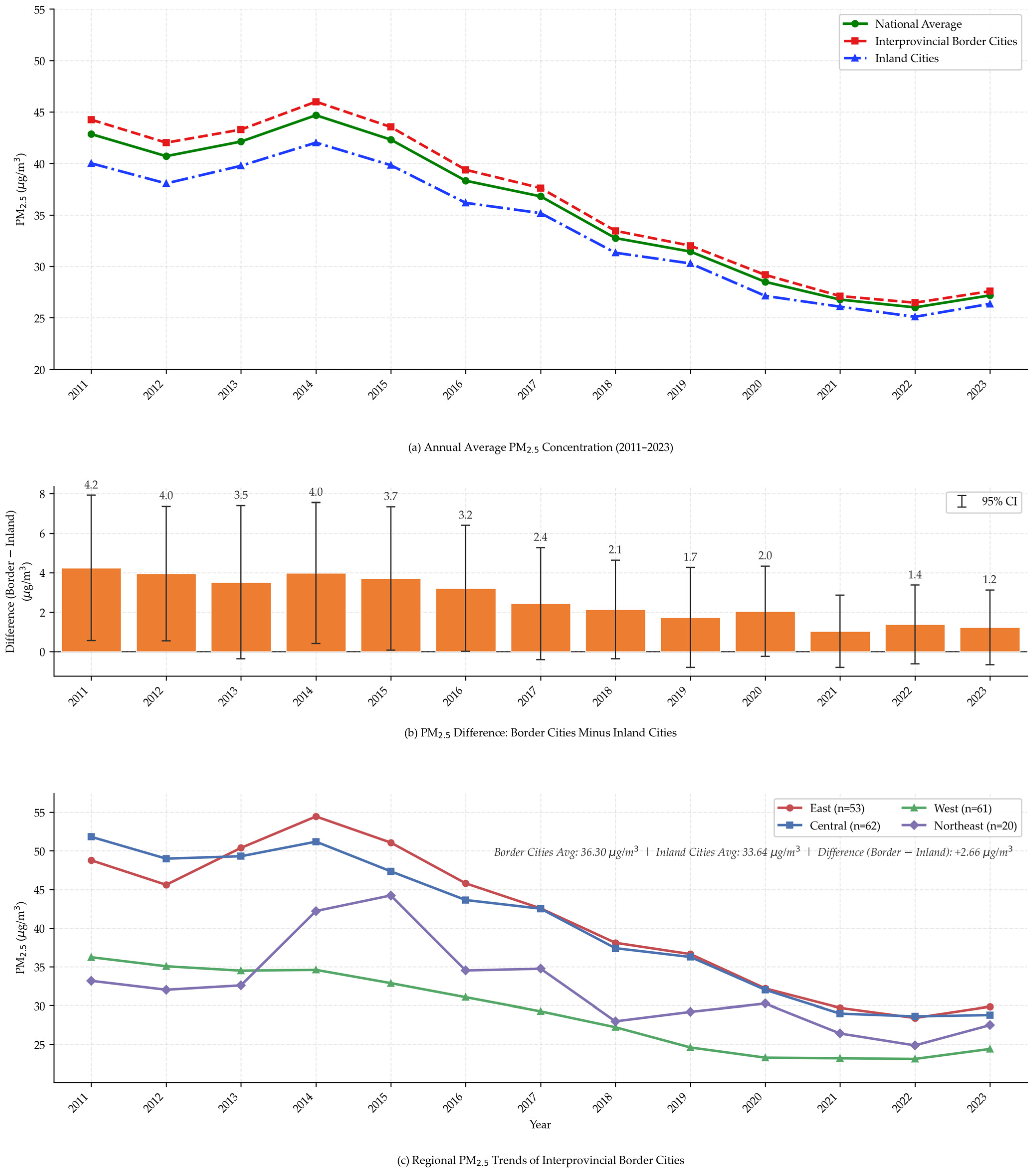
Figure 1. Border cities versus inland cities.
Sustainability 18 08668 g001
Figure 2. Mechanism analysis diagram.
Sustainability 18 08668 g002
Figure 3. Green patent collaboration network among boundary cities.
Sustainability 18 08668 g003
Figure 4. Spatial distribution of prefecture-level cities along inter-provincial administrative boundary areas.
Sustainability 18 08668 g004
Figure 5. Inter-provincial boundary exposure intensity.
Sustainability 18 08668 g005
Table 1. Descriptive statistics.
VariableDefinitionNMeanStd. DevMinMax
PollutionDependent variable38093.48160.44590.72904.5292
GICGTIGreen innovation collaboration38093.07711.81320.00009.4390
GTL38092.40101.77600.00008.8568
BorderBoundary exposure intensity38090.12070.12010.00000.6163
GTI x BorderExplanatory variable38090.36890.52970.00003.7818
GLI x Border38090.28460.45960.00003.5485
DensityPopulation density38095.60191.20990.15079.0948
FlowPopulation mobility38090.00740.3438−0.46844.2027
PgdpEconomic development380910.78530.54948.806812.4817
OpenOpenness38090.18090.28870.00002.5474
HumanHuman capital38090.01990.02190.00000.1666
FinanceFinancial development38092.75921.34450.587921.3047
GovGovernment intervention38090.22510.14540.0561.6649
MobileMobile phone penetration38091.10010.72700.19259.7920
TechScience and technology level38090.00300.00260.00000.0220
Table 2. Baseline regression results.
Variable(1)(2)(3)(4)(5)(6)(7)(8)
PollutionPollutionPollutionPollutionPollutionPollutionPollutionPollution
GTI × Border−0.0565 ***
(0.0201)
−0.0369 **
(0.0186)
GLI × Border −0.0459 **
(0.0182)
−0.0312 *
(0.0168)
WGTI × Border −0.0591 ***
(0.0219)
−0.0378 **
(0.0202)
WGLI × Border −0.0486 **
(0.0206)
−0.0319 *
(0.0193)
Density −0.1670 ***
(0.0611)
−0.1655 ***
(0.0612)
−0.1659 ***
(0.0611)
−0.1641 ***
(0.0613)
Flow 0.1700 ***
(0.0569)
0.1705 ***
(0.0573)
0.1700 ***
(0.0570)
0.1704 ***
(0.0573)
Pgdp −0.1146 ***
(0.0345)
−0.1173 ***
(0.0345)
−0.1153 ***
(0.0346)
−0.1177 ***
(0.0346)
Open −0.0738 ***
(0.0277)
−0.0744 ***
(0.0276)
−0.0739 ***
(0.0276)
−0.0746 ***
(0.0276)
Human −0.6911
(0.5961)
−0.6767
(0.5958)
−0.6820
(0.5949)
−0.6680
(0.5949)
Finance −0.0213 **
(0.0100)
−0.0216 **
(0.0100)
−0.0214 **
(0.0100)
−0.0216 **
(0.0100)
Gov 0.0112
(0.0885)
0.0105
(0.0887)
0.0115
(0.0886)
0.0112
(0.0888)
Mobile −0.0484 ***
(0.0171)
−0.0485 ***
(0.0172)
−0.0484 ***
(0.0171)
−0.0485 ***
(0.0172)
Tech −12.2127 ***
(2.0511)
−12.2543 ***
(2.0603)
−12.2216 ***
(2.0507)
−12.2808 ***
(2.0638)
ControlsNONOYESYESNONOYESYES
Year FEYESYESYESYESYESYESYESYES
City FEYESYESYESYESYESYESYESYES
R20.95360.95350.95710.95700.95360.95350.95700.9570
N38093809380938093809380938093809
Note: Robust standard errors clustered at the city level are reported in parentheses. *** p < 0.01, ** p < 0.05, * p < 0.1.
Table 3. Robustness checks I.
Variable(1)(2)(3)(4)(5)(6)(7)(8)(9)(10)
Alternative Explanatory Variables
Border = 20 kmBorder = 20 kmBorder = 30 kmBorder = 30 kmBorder = 0/1Border = 0/1PollutionPollutionPollutionPollution
GTI × Border−0.0206 **
(0.0104)
−0.0159 **
(0.0076)
−0.0088 **
(0.0037)
GLI × Border −0.0168 *
(0.0094)
−0.0126 *
(0.0069)
−0.0059 *
(0.0033)
GTII × Border −0.0301 *
(0.0183)
GTUI × Border −0.0385 **
(0.0166)
GLII × Border −0.0286 *
(0.0174)
GLUI × Border −0.0357 **
(0.0157)
ControlsYESYESYESYESYESYESYESYESYESYES
Year FEYESYESYESYESYESYESYESYESYESYES
City FEYESYESYESYESYESYESYESYESYESYES
R20.95710.95700.95710.95700.95710.95700.95700.95710.95700.9570
N3809380938093809380938093809380938093809
Note: Robust standard errors clustered at the city level are reported in parentheses.** p < 0.05, * p < 0.1.
Table 4. Robustness checks II.
Variable(1)(2)(3)(4)(5)(6)(7)(8)(9)(10)
Replace the Explained VariableJoint Prevention and Control of Air PollutionPollution Rights Trading Pilot Program
Pollution-DPollution-DPM2.5PM2.5SO2SO2PollutionPollutionPollutionPollution
GTI x Border−0.0369 **
(0.0186)
−2.7688 ***
(1.002)
−0.1814 *
(0.0997)
−0.0343 *
(0.0185)
−0.0369 **
(0.0186)
GLI x Border −0.0313 *
(0.0168)
−2.2995 **
(0.9748)
−0.1566 *
(0.0852)
−0.0287 *
(0.0168)
−0.0313 *
(0.0168)
ControlsYESYESYESYESYESYESYESYESYESYES
Year FEYESYESYESYESYESYESYESYESYESYES
City FEYESYESYESYESYESYESYESYESYESYES
R20.91960.91960.90930.90900.90160.90150.95720.95720.95710.9571
N3809380938093809372537253757375738093809
Note: Robust standard errors clustered at the city level are reported in parentheses. *** p < 0.01, ** p < 0.05, * p < 0.1.
Table 5. Robustness checks III.
Variable(1)(2)(3)(4)(5)(6)(7)(8)(9)(10)
National Air Ten-Year PlanCarbon Emission Rights Trading Pilot Policy1% Winsorization5% WinsorizationAdd the Nighttime Light Data
PollutionPollutionPollutionPollutionPollutionPollutionPollutionPollutionPollutionPollution
GTI × Border−0.0305 *
(0.0181)
−0.0316 *
(0.0181)
−0.0294 *
(0.0175)
−0.0283 *
(0.0172)
−0.0357 *
(0.0184)
GLI × Border −0.0273 *
(0.0166)
−0.0269 *
(0.0163)
−0.0257 *
(0.0156)
−0.0248 *
(0.0151)
−0.0289 *
(0.0165)
ControlsYESYESYESYESYESYESYESYESYESYES
Year FEYESYESYESYESYESYESYESYESYESYES
City FEYESYESYESYESYESYESYESYESYESYES
R20.95610.95610.95670.95670.95430.95430.94290.94280.95760.9575
N3809380938093809380938093809380938093809
Note: Robust standard errors clustered at the city level are reported in parentheses. * p < 0.1.
Table 6. Instrumental variable method.
Variable(1)(2)(3)(4)(5)(6)(7)(8)
First StageSecond StageFirst StageSecond StageFirst StageSecond StageFirst StageSecond Stage
GTI × BorderPollutionGLI × BorderPollutionGTI × BorderPollutionGLI × BorderPollution
GTI × Border −6.1486 ***
(2.0231)
−9.0541 ***
(3.0089)
GLI × Border −6.6509 ***
(2.3305)
−10.1364 ***
(3.3726)
IV10.5723 ***
(0.0269)
IV2 0.4715 ***
(0.0315)
IV3 0.4470 ***
(0.0316)
IV4 0.3455 ***
(0.0315)
ControlsYESYESYESYESYESYESYESYES
Year FEYESYESYESYESYESYESYESYES
City FEYESYESYESYESYESYESYESYES
KP rk LM53.176 ***
(0.0000)
51.869 ***
(0.0000)
47.289 ***
(0.0000)
51.589 ***
(0.0000)
KP rk Wald F451.232 223.985 199.698 120.037
N35163516351635163223322332233223
Note: Robust standard errors clustered at the city level are reported in parentheses. *** p < 0.01.
Table 7. Heckman method.
Variable(1)(2)(3)(4)
First StageSecond StageFirst StageSecond Stage
Coop_GPollutionCoop_LPollution
GTI × Border −0.0312 *
(0.0165)
GLI × Border −0.0447 **
(0.0180)
IMR −0.0792 ***
(0.0258)
−0.0979 ***
(0.0265)
HistoryCoop0.3841 ***
(0.0316)
0.4354 ***
(0.0438)
ControlsYESYESYESYES
Year FEYESYESYESYES
City FENOYESNOYES
R20.95620.9563
N3796379635043504
Note: Robust standard errors clustered at the city level are reported in parentheses. *** p < 0.01, ** p < 0.05, * p < 0.1.
Table 8. Estimation results of global Moran’s I index for each year.
YearMoran’s IZ-Valuep-Value
20110.450511.15150.0005
20120.476710.95590.0005
20130.525212.55320.0005
20140.439411.00460.0005
20150.485311.75580.0005
20160.497811.65150.0005
20170.430610.96040.0005
20180.474511.28950.0005
20190.47111.30210.0005
20200.472311.51480.0005
20210.414110.37530.0005
20220.45210.90790.0005
20230.391410.30260.0005
Note: p-values are based on 1999 random permutations.
Table 9. Spatial Durbin model results.
Variables(1)(2)
GTI × BorderGLI × Border
Main effect−0.0186 ***
(0.0053)
−0.0164 ***
(0.0053)
W × (GIC × Border)−0.0278 ***
(0.0107)
−0.0230 **
(0.0107)
Direct effect−0.0401 ***
(0.0085)
−0.0346 ***
(0.0084)
Indirect effect−0.3159 ***
(0.0787)
−0.2679 ***
(0.0779)
Total effect−0.3560 ***
(0.0855)
−0.3025 ***
(0.0846)
ρ0.8761 ***
(0.0077)
0.8763 ***
(0.0077)
C o n t r o l s YESYES
S p a t i a l   l a g   o f   c o n t r o l s YESYES
ControlsYESYES
Year FEYESYES
City FE38093809
Within R20.71150.7100
Note: Robust standard errors clustered at the city level are reported in parentheses. *** p < 0.01, ** p < 0.05.
Table 10. Heterogeneity in analysis.
VariablePollution PressureFiscal PressureOpenness
(1)(2)(3)(4)(5)(6)
GTI × BorderGLI × BorderGTI × BorderGLI × BorderGTI × BorderGLI × Border
Core effect: Low group0.0204
(0.0240)
0.0232
(0.0234)
−0.0720 ***
(0.0261)
−0.0618 **
(0.0254)
−0.0199
(0.0204)
−0.014
(0.0186)
Core × High group−0.0897 ***
(0.0306)
−0.0860 ***
(0.0289)
0.0544 *
(0.0299)
0.0481 *
(0.0286)
−0.0587 *
(0.0313)
−0.0514 *
(0.0285)
Total effect: High group−0.0692 ***
(0.0247)
−0.0628 ***
(0.0220)
−0.0176
(0.0209)
−0.0137
(0.0187)
−0.0786 ***
(0.0286)
−0.0655 **
(0.0254)
GIC × Border × East
Core effect: Low group−0.0576 ***
(0.0091)
−0.0593 ***
(0.0097)
−0.0458 ***
(0.0088)
−0.0449 ***
(0.0102)
−0.0482
(0.0498)
−0.0216
(0.0601)
Core × High group0.0227
(0.0164)
0.0241
(0.0177)
−0.0113
(0.0169)
−0.0148
(0.0181)
−0.0022
(0.0502)
−0.0298
(0.0604)
Total effect: High group−0.0349 **
(0.0142)
−0.0353 **
(0.0154)
−0.0571 ***
(0.0144)
−0.0597 ***
(0.0151)
−0.0504 ***
(0.0071)
−0.0514 ***
(0.0077)
GIC × Border × Central
Core effect: Low group0.0310
(0.0676)
0.0045
(0.0575)
−0.0004
(0.0060)
−0.0034
(0.0069)
0.0126
(0.0117)
0.0060
(0.0092)
Core × High group−0.0208
(0.0683)
−0.0004
(0.0590)
0.0561**
(0.0276)
0.0318
(0.0257)
−0.0187
(0.0346)
−0.0175
(0.0366)
Total effect: High group0.0102
(0.0101)
0.0041
(0.0087)
0.0557**
(0.0270)
0.0284
(0.0246)
−0.0060
(0.0329)
−0.0115
(0.0353)
GIC × Border × Western
Core effect: Low group−0.0370 ***
(0.0103)
−0.0411 ***
(0.0107)
−0.0538 ***
(0.0093)
−0.0571 ***
(0.0100)
−0.0323 **
(0.0132)
−0.0266 **
(0.0112)
Core × High group−0.0015
(0.0240)
0.0138
(0.0173)
0.0210
(0.0152)
0.0240
(0.0156)
−0.0165
(0.0175)
−0.0397 **
(0.0152)
Total effect: High group−0.0385 *
(0.0225)
−0.0273 *
(0.0145)
−0.0328 ***
(.0123)
−0.0332 ***
(0.0120)
−0.0488 ***
(0.0113)
−0.0664 ***
(0.0105)
GIC × Border × Northeastern
Core effect: Low group−0.0132 **
(0.0063)
−0.0144 **
(0.0064)
−0.0131 ***
(0.0048)
−0.0148 ***
(0.0052)
−0.0149 **
(0.0065)
−0.0159 **
(0.0061)
Core × High group−0.8695 ***
(0.2111)
−0.4935 **
(0.2159)
0.0351 ***
(0.0082)
0.0378
(0.0084)
0.0018
(0.0141)
0.0023
(0.0148)
Total effect: High group−0.8827 ***
(0.2115)
−0.5079 **
(0.2163)
0.0220 ***
(0.0064)
0.0230 ***
(0.0062)
−0.0131
(0.0121)
−0.0136
(0.0130)
ControlsYESYESYESYESYESYES
Year FEYESYESYESYESYESYES
City FEYESYESYESYESYESYES
Note: Robust standard errors clustered at the city level are reported in parentheses. *** p < 0.01, ** p < 0.05, * p < 0.1.
Table 11. Mechanism analysis.
VariableCOGCOGPollutionPollutionISUISUPollutionPollution
(1)(2)(3)(4)(5)(6)(7)(8)
GTI × Border0.1952 ***
(0.0359)
−0.0369 **
(0.0062)
0.0406 ***
(0.0008)
−0.0387 ***
(0.0072)
GLI × Border 0.2038 ***
(0.0382)
−0.0394 ***
(0.0065)
0.0447 ***
(0.0073)
−0.0411 ***
(0.0075)
COG −0.0335 ***
(0.0056)
−0.0336 ***
(0.0056)
ISU −0.1178 ***
(0.0343)
−0.1159 ***
(0.0345)
ControlsYESYESYESYESYESYESYESYES
Year FEYESYESYESYESYESYESYESYES
City FEYESYESYESYESYESYESYESYES
N36153615361536153615361536153615
Note: Robust standard errors clustered at the city level are reported in parentheses. *** p < 0.01, ** p < 0.05.
Table 12. Analysis of parallel mediating effect.
VariablesGTI × BorderGLI × Border
Indirect effect: COG−0.0064 ***
(0.0017)
−0.0067 ***
(0.0018)
BC 95% CI[−0.0103, −0.0035][−0.0107, −0.0037]
Indirect effect: ISU−0.0046 ***
(0.0015)
−0.0050 ***
(0.0017)
BC 95% CI[−0.0082, −0.0021][−0.0087, −0.0022]
Total indirect effect−0.0111 ***
(0.0023)
−0.0117 ***
(0.0023)
BC 95% CI[−0.0161, −0.0072][−0.0168, −0.0074]
Direct effect−0.0324 ***
(0.0066)
−0.0345 ***
(0.0070)
BC 95% CI[−0.0461, −0.0198][−0.0497, −0.0216]
Total effect−0.0435 ***
(0.0066)
−0.0463 ***
(0.0069)
BC 95% CI[−0.0560, −0.0291][−0.0600, −0.0322]
Share of COG path58.16% ***
(10.75%)
57.31% ***
(11.06%)
Share of industrial upgrading path41.84% ***
(10.75%)
42.69% ***
(11.06%)
Observations36153615
Bootstrap replications10001000
Note: Robust standard errors clustered at the city level are reported in parentheses. *** p < 0.01.
Table 13. Chain mediation effect analysis.
VariablesGTI × BorderGLI × Border
Indirect effect: COG−0.0064 ***
(0.0017)
−0.0067 ***
(0.0018)
BC 95% CI[−0.0103, −0.0035][−0.0107, −0.0037]
Indirect effect: ISU−0.0045 ***
(0.0015)
−0.0049 ***
(0.0016)
BC 95% CI[−0.0080, −0.0020][−0.0086, −0.0021]
Chain effect: COG → ISU−0.0001
(0.0001)
−0.0001
(0.0001)
BC 95% CI[−0.0004, 0.0001][−0.0004, 0.0001]
Total indirect effect−0.0111 ***
(0.0023)
−0.0117 ***
(0.0023)
BC 95% CI[−0.0161, −0.0072][−0.0168, −0.0074]
Direct effect−0.0324 ***
(0.0066)
−0.0345 ***
(0.0070)
BC 95% CI[−0.0461, −0.0198][−0.0497, −0.0216]
Observations36153615
Bootstrap replications10001000
Note: Robust standard errors clustered at the city level are reported in parentheses. *** p < 0.01.
Table 14. Group-specific parallel mediation effects.
Grouping DimensionGroupGIC × BorderCollaborative-Governance ContributionIndustrial-Upgrading Contribution
Pollution pressureLowGTI × Border−0.0076 (70.42%)−0.0032 (29.58%)
GLI × Border−0.0082 (70.19%)−0.0035 (29.81%)
HighGTI × Border−0.0020 (44.94%)−0.0024 (55.06%)
GLI × Border−0.0018 (41.21%)−0.0025 (58.79%)
Fiscal pressureLowGTI × Border−0.0034 (43.90%)−0.0044 (56.10%)
GLI × Border−0.0037 (44.91%)−0.0045 (55.09%)
HighGTI × Border−0.0084 (67.48%)−0.0040 (32.52%)
GLI × Border−0.0087 (66.38%)−0.0044 (33.62%)
OpennessLowGTI × Border−0.0062 (55.51%)−0.0049 (44.49%)
GLI × Border−0.0062 (51.02%)−0.0059 (48.98%)
HighGTI × Border−0.0061 (62.97%)−0.0036 (37.03%)
GLI × Border−0.0065 (63.72%)−0.0037 (36.28%)
Disclaimer/Publisher’s Note: The statements, opinions and data contained in all publications are solely those of the individual author(s) and contributor(s) and not of MDPI and/or the editor(s). MDPI and/or the editor(s) disclaim responsibility for any injury to people or property resulting from any ideas, methods, instructions or products referred to in the content.