Spatiotemporal Patterns of Landscape Ecological Risk and Their Driving Mechanisms in Xinzhou City, Shanxi Province, China

Abstract

Understanding spatiotemporal changes in landscape ecological risk is essential for regional ecological security and sustainable land management, particularly in environmentally sensitive areas. Using land-use data from five time points (2000, 2005, 2010, 2015, and 2020) together with topographic, climatic, vegetation, and socioeconomic data, we assessed landscape ecological risk dynamics in Xinzhou City, a typical ecologically sensitive region in the middle Yellow River Basin. We integrated a landscape ecological risk assessment model, spatial autocorrelation analysis, and an optimal-parameter geographical detector (OPGD) to identify the spatiotemporal patterns and key drivers of ecological risk. Built-up land expanded by 131.47% over the study period, while cropland and grassland both contracted. Land-use change was dominated by bidirectional conversion between cropland and grassland, alongside a net shift of both to built-up land. Overall, ecological risk declined: high- and relatively high-risk areas decreased by 1354.15 km². Spatially, the pattern remained stable, with higher risk in basins and lower risk in mountainous regions, although the trend varied across phases. Risk exhibited significant spatial clustering: low–low clusters remained stable in mountainous ecological source areas, whereas high–high clusters persisted in basin agricultural areas. Elevation was the dominant factor in spatial risk differentiation. Combined natural and anthropogenic factors shaped the overall risk pattern. Despite the regional decline, urbanization-induced disturbance remains the principal driver of local risk increases. Our findings demonstrate the value of coupling long-term land-use data with OPGD to evaluate the relative and interactive contributions of terrain constraints and anthropogenic drivers in complex mountain–basin systems, with implications for spatially targeted ecological restoration and sustainable land management in ecologically sensitive transition zones.

1. Introduction

Landscape ecological risk encompasses the potential for landscape pattern degradation and impaired ecosystem structure and function under the combined pressures of environmental change and human activity. It lies at the nexus of landscape ecology and regional ecological risk assessment [1,2,3]. Globally, land-use patterns are undergoing continuous transformation driven by climate change and intensifying human disturbance. Landscape fragmentation is increasing, ecosystem services are degrading, and these trends are imposing growing constraints on regional ecological security and sustainable development [4,5,6]. Against this backdrop, elucidating the spatiotemporal dynamics of landscape ecological risk has become a practical priority for territorial spatial planning and ecological protection. Furthermore, identifying the factors that drive its spatial variation can directly inform targeted risk management and adaptive land-use policies [7,8].

The ecological risk assessment paradigm has undergone a marked shift from single-pollutant toxicity evaluation to integrated multi-factor analysis [9]. Since the 1990s, advances in landscape ecology theory and spatial analysis techniques have enabled the integration of landscape pattern indices into risk studies, gradually establishing an assessment framework centered on landscape disturbance and vulnerability, underpinned by land-use data [10,11,12]. Empirical applications of this framework have extended across river basins [13,14], plateaus [15,16], urban agglomerations [17,18], and mining areas [19], providing systematic documentation of ecological risk dynamics across diverse settings. Both natural and socioeconomic factors are widely recognized as joint drivers of spatial risk variation [20,21]. Research is consequently advancing beyond pattern characterization toward integrated analyses of pattern, process, and mechanism [22,23,24]. However, many existing studies still rely on traditional correlation or regression methods that assume spatial stationarity, which often fail to capture the spatially varying relationships between natural and anthropogenic drivers. Although geographically weighted regression (GWR) and other non-stationary techniques have been increasingly adopted to model local spatial variation, these methods primarily address continuous response surfaces and do not directly quantify the discrete explanatory power of individual factors or their interactions. Geographical detectors offer a complementary approach: they quantify both individual factor effects and their interactive influences, assess the relative contributions of drivers after optimal discretization, and detect pairwise interactions—all without requiring distributional assumptions. Whereas GWR models the continuous spatial variation in regression coefficients, OPGD measures the explanatory power of discretized factors and identifies whether two factors interact to amplify or attenuate their effects on spatial risk differentiation [25].

The Yellow River Basin serves as a core ecological barrier in northern China and a key economic belt. Its ecological protection and high-quality development have been designated as a national strategy [26]. Xinzhou City lies in north-central Shanxi Province on the eastern Loess Plateau, where the ecologically sensitive middle Yellow River Basin meets the northern farming-pastoral ecotone. It occupies a pivotal position within the basin’s ecological security network [27]. The region is characterized by severe soil erosion, high precipitation variability, and fragile ecosystems where small land-use changes can trigger disproportionate ecological consequences [28]. In recent years, accelerated urbanization and sustained mineral extraction in Shanxi—a major coal-producing province—have significantly altered local land-use patterns and intensified pressures on regional ecosystems [29]. Existing studies in this region have focused primarily on cultivated land security [30] or land-use zoning [31]. Although these efforts provide valuable site-specific insights, the broader landscape-scale risk dynamics and their spatial drivers in Xinzhou remain poorly understood, particularly the relative and interactive contributions of terrain constraints and anthropogenic disturbance.

This study advances existing assessments in the middle Yellow River Basin by integrating an optimal-parameter geographical detector (OPGD) with a landscape ecological risk assessment model to explicitly evaluate the effects of terrain constraints from those of anthropogenic disturbance in a typical mountain–basin system. Using land-use data from five snapshot years (2000, 2005, 2010, 2015, and 2020), this study seeks to answer three research questions (RQs): (RQ1) How has landscape ecological risk in Xinzhou City evolved spatially and temporally from 2000 to 2020? (RQ2) How are high- and low-risk zones spatially clustered, and how has this clustering changed? (RQ3) Which factors dominate the spatial differentiation of ecological risk, and how do they interact? The answers to these questions are expected to inform territorial spatial optimization and ecological risk management in the region and contribute to SDG 15 (Life on Land) and SDG 11 (Sustainable Cities and Communities).

2. Materials and Methods

2.1. Study Area and Data Sources

2.1.1. Study Area

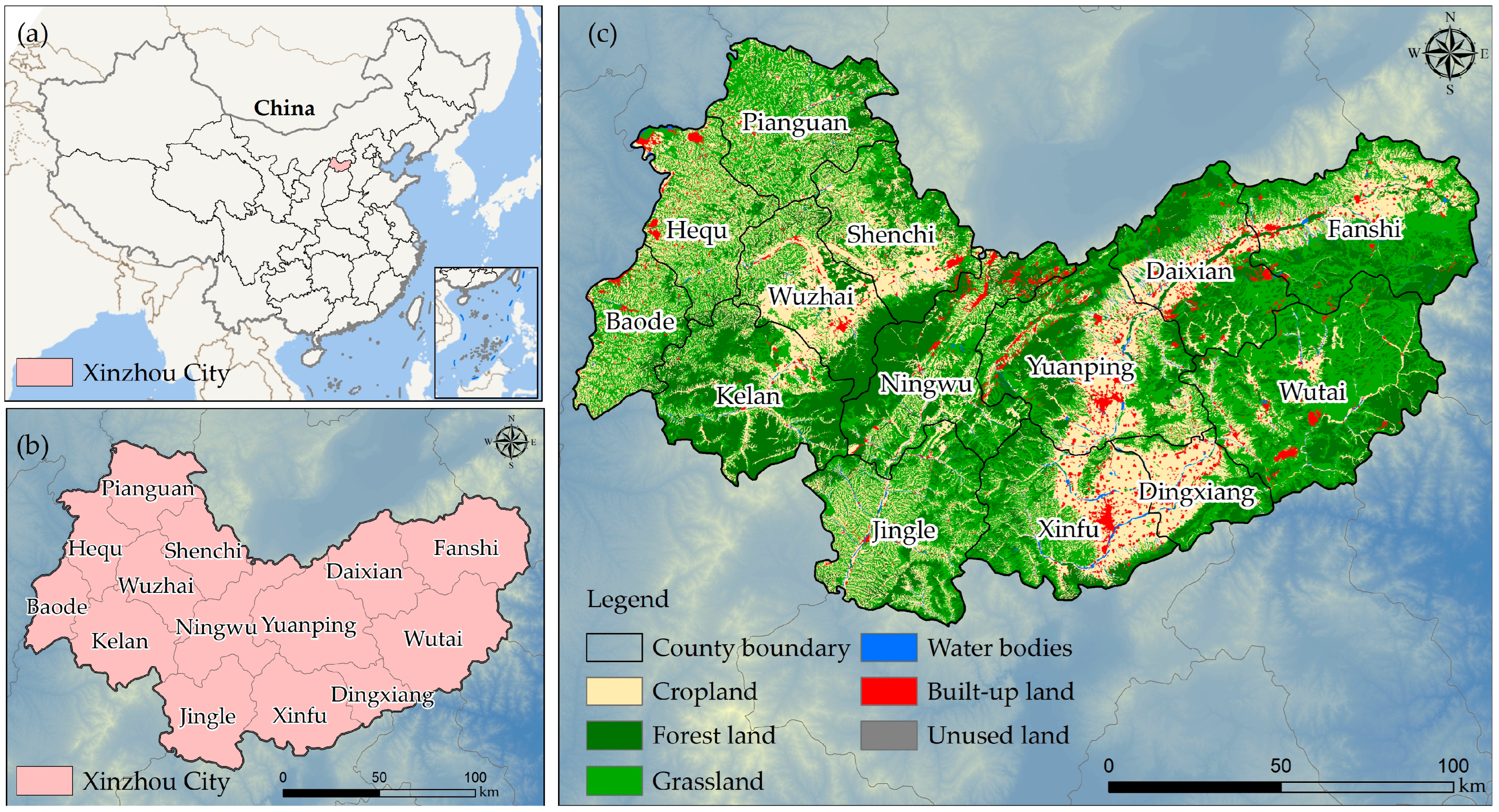
Xinzhou City covers 25,152 km², making it the largest prefecture-level city in Shanxi Province. Mountains and hills dominate the terrain, jointly accounting for over 89% of the total area, while the central Xin-Ding Basin forms the core agricultural zone. The region experiences a temperate continental monsoon climate and hosts a dense river network fed by the Yellow, Hutuo, and Sanggan River systems (Figure 1). This physical setting makes Xinzhou particularly suitable for examining landscape ecological risk dynamics.

2.1.2. Data Sources and Processing

This study utilizes four categories of data: land use, natural environment, socioeconomic factors, and locational factors. Land-use data were obtained from the Resource and Environmental Science Data Center of the Chinese Academy of Sciences (RESDC, http://www.resdc.cn). To reflect the terrain characteristics of Xinzhou’s mountainous and hilly Loess Plateau setting, we reclassified the original land-use types into six broad categories: cropland, forest land, grassland, water bodies, built-up land, and unused land. DEM, NDVI, population density, and GDP data were obtained from the same platform. Slope was derived from the DEM via GIS-based terrain analysis. Annual precipitation and night-time light data were downloaded from the National Earth System Science Data Center (https://www.geodata.cn). For locational factors, we extracted built-up land and rural settlement layers from the land-use data and generated Euclidean distance rasters to represent the varying ecological impacts of urban expansion and rural settlement development. All datasets were projected to the same coordinate system, clipped to the study area boundary, and resampled to 30 m spatial resolution (

Table 1. Data sources.

Data Type	Data Name	Original Resolution	Resampled Resolution	Data Source
Land use data	Land use data	30 m	30 m	Resource and Environmental Science Data Center, Chinese Academy of Sciences (http://www.resdc.cn) (accessed on 15 March 2024)
Natural environment data	DEM	250 m	30 m	Resource and Environmental Science Data Center, Chinese Academy of Sciences (http://www.resdc.cn) (accessed on 15 March 2024)
	Slope	250 m	30 m	Derived from DEM
	NDVI	1000 m	30 m	Resource and Environmental Science Data Center, Chinese Academy of Sciences (http://www.resdc.cn) (accessed on 10 January 2025)
	Annual precipitation	1000 m	30 m	National Earth System Science Data Center (https://www.geodata.cn) (accessed on 10 January 2025)
Socioeconomic data	Population density	1000 m	30 m	Resource and Environmental Science Data Center, Chinese Academy of Sciences (http://www.resdc.cn) (accessed on 16 March 2024)
	GDP	1000 m	30 m	Resource and Environmental Science Data Center, Chinese Academy of Sciences (http://www.resdc.cn) (accessed on 23 September 2024)
	Nighttime light data	1000 m	30 m	National Earth System Science Data Center (https://www.geodata.cn) (accessed on 24 September 2024)
Location condition data	Distance to built-up land	1000 m	30 m	Derived from land use data
	Distance to rural settlements	1000 m	30 m	Derived from land use data

Note: All original raster datasets were resampled to a uniform 30 m resolution. Categorical data (land use) were resampled using the nearest-neighbor method to preserve class boundaries; continuous data (DEM, NDVI, precipitation, population density, GDP, nighttime light) were resampled using bilinear interpolation.

).

2.2. Research Methods

2.2.1. Land Use Transfer Matrix

The land-use transfer matrix is a fundamental quantitative method for analyzing land-use changes, systematically revealing spatiotemporal conversions among different land-use types [32]. The transfer matrix is expressed as:

$$S_{ij}=\left\{\begin{array}{c}\begin{array}{c}\begin{array}{c}{S}_{11} S_{12} \dots S_{1n}\\ S_{21} S_{22} \dots S_{2n}\end{array}\\ ⋮ ⋮ ⋮ ⋮\end{array}\\ S_{n1} S_{n2} \dots S_{nn}\end{array}\right\}$$

(1)

where $\mathrm{S}$ is the land use area, $\mathrm{i}$ and $\mathrm{j}$ denote the land use types at the beginning and end of the study period, respectively, and ${\mathrm{S}}_{\mathrm{i}\mathrm{j}}$ is the area converted from type $\mathrm{i}$ to type $\mathrm{j}$ during the study period. Row elements represent outward conversions from type $\mathrm{i}$, whereas column elements represent inward conversions into type $\mathrm{j}$, Diagonal elements indicate the area that remained unchanged [33].

2.2.2. Landscape Ecological Risk Assessment Model

Evaluation Unit Division

Using the Create Fishnet tool in ArcGIS 10.8, the study area was divided into regular spatial units (3 km × 3 km grids), resulting in 2996 evaluation units. This grid size was selected for three reasons. First, landscape ecological risk assessment operates at the landscape pattern level rather than the pixel level; the 3 km grid effectively captures spatial heterogeneity in mountain–basin terrain, where land-use patches typically range from 0.5 to 5 km². Second, this resolution provides a sufficient number of evaluation units (n = 2996) for robust spatial autocorrelation and geographical detector analyses. Third, the selected grid size is consistent with those commonly adopted in prefecture-level landscape ecological risk assessments (1–5 km) [34,35,36]. The 30 m resolution data were retained as the base input for land-use classification and landscape index calculation within each grid, while the 3 km grid aggregates these fine-scale patterns into meaningful landscape-level metrics.

Landscape Ecological Risk Index Construction

The Ecological Risk Index (ERI) integrates landscape disturbance and vulnerability to represent the relative magnitude of ecological loss of different landscape types under external disturbances. Following established frameworks [37], the ERI for each evaluation unit is calculated as:

$$ERI={\displaystyle \sum _{i=1}^n}{\displaystyle \frac{A_{mi}}{A_k}}{R}_i$$

(2)

where $\mathrm{E}\mathrm{R}\mathrm{I}$ is the landscape ecological risk index (higher values indicate higher risk), $\mathrm{n}$ is the number of landscape types in the unit, ${\mathrm{A}}_{\mathrm{m}\mathrm{i}}$ is the area of landscape type $\mathrm{i}$ in unit $\mathrm{m}$, ${\mathrm{A}}_{\mathrm{k}}$ is the area of the unit, and ${\mathrm{R}}_{\mathrm{i}}$ is the landscape loss index.

Following the established vulnerability ranking from highest to lowest (unused land, water bodies, cropland, grassland, forest land, and built-up land), we assigned ordinal values of 6, 5, 4, 3, 2, and 1, respectively, which were then normalized to obtain the following Fi values: unused land = 1.0, water bodies = 0.8, cropland = 0.6, grassland = 0.4, forest land = 0.2, and built-up land = 0.1. The ERI is an area-weighted aggregate computed over the entire 3 km × 3 km evaluation unit, rather than a per-patch measure. Therefore, although built-up land receives the lowest Fi, it can still dominate high-risk grids because its extensive areal coverage (>80% in urban cores) amplifies its aggregate contribution to the ERI. Concurrently, the absence of forest and grassland patches removes any risk-mitigating effect.

Landscape disturbance index ${\mathrm{E}}_{\mathrm{i}}$ is computed as:

$$E_i=a{C}_i+b{N}_i+c{D}_i$$

(3)

where ${\mathrm{C}}_{\mathrm{i}}$, N_i, and D_i are the landscape fragmentation, isolation, and dominance indices, respectively, with weights a = 0.5, b = 0.3, and c = 0.2 based on previous studies.

We ranked landscape vulnerability Fi from highest to lowest as: unused land, water bodies, cropland, grassland, forest land, and built-up land, and then normalized the values.

The landscape loss index is:

$$R_i=E_i\times F_i$$

(4)

Detailed definitions and formulas for each index are provided in

Table 2. Formulas and definitions of landscape risk indices.

Landscape Index	Formula	Meaning
Landscape disturbance index Ei	Ei = aCi + bNi + cDi	Reflects the degree of external disturbance experienced by different landscape types, obtained as a weighted sum of fragmentation index (Ci), isolation index (Ni), and dominance index (Di). The weights a, b, and c are assigned values of 0.5, 0.3, and 0.2, respectively, following previous studies, with a + b + c = 1.
Landscape loss index Ri	Ri = Ei × Fi	—
Landscape vulnerability index Fi	Normalized value	Characterizes the ability of different landscape types to resist external disturbance. Higher values indicate greater susceptibility to ecological degradation. Based on the study area and previous research, vulnerability levels from highest to lowest are: unused land, water bodies, cropland, grassland, forest land, and built-up land. These are then normalized to obtain Fi.
Landscape fragmentation index Ci	${\mathrm{C}}_{\mathrm{i}}={\displaystyle \frac{{\mathrm{n}}_{\mathrm{i}}}{{\mathrm{A}}_{\mathrm{i}}}}$	Where ni is the number of patches of landscape type i, and Ai is its total area. A larger Ci suggests a higher degree of fragmentation.
Landscape isolation index Ni	${\mathrm{N}}_{\mathrm{i}}={\displaystyle \frac{\mathrm{A}}{{2\mathrm{A}}_{\mathrm{i}}}}\sqrt{{\displaystyle \frac{{\mathrm{n}}_{\mathrm{i}}}{\mathrm{A}}}}$	Where ni is the number of patches of type i, Ai is its total area, and A is the total landscape area. A larger Ni suggests more dispersed patches and poorer connectivity.
Landscape dominance index Di	${\mathrm{D}}_{\mathrm{i}}={\displaystyle \frac{{\mathrm{Q}}_{\mathrm{i}}+{\mathrm{M}}_{\mathrm{i}}}{4}}+{\displaystyle \frac{{\mathrm{L}}_{\mathrm{i}}}{2}}$	Where Qi is the proportion of quadrats containing type i to the total number of quadrats Mi is the proportion of patches of type i to the total number of patches, andLi is the proportion of the area of type i to the total landscape area. A larger Di suggests a more dominant position of the landscape type in the overall pattern.

Note: All equations presented in this table are derived from established landscape ecological risk assessment frameworks.

.

Spatial Interpolation and Risk Grading

We used the ERI values at the center of each evaluation unit as sample points and performed ordinary kriging interpolation in ArcGIS 10.8 to generate a continuous spatial distribution map of landscape ecological risk across the study area. The interpolated results were classified into five risk levels (low, relatively low, medium, relatively high, and high) using the Jenks natural breaks method. The kriging-interpolated risk surfaces were used solely for visualization and risk-level mapping; all quantitative analyses—including spatial autocorrelation and OPGD factor detection—were performed directly on the original ERI values of the 2996 grid cells.

2.2.3. Spatial Autocorrelation Analysis

Spatial autocorrelation analysis was conducted using GeoDa software (software version number is 1.16.0.16) at both global and local scales. The global Moran’s I index measures the overall spatial correlation of landscape ecological risk:

$$I = {\displaystyle \frac{n{\sum }_{i=1}^n{\displaystyle {\sum }_{j=1}^n}{w}_{ij}\left(x_i-\overline{x}\right)\left(x_j-\overline{x}\right)}{n{\sum }_{i=1}^n{\displaystyle {\sum }_{j=1}^n}{w}_{ij}{\displaystyle {\sum }_{i=1}^n}\left(x_j-\overline{x}\right)\text{²}}}$$

(5)

where n is the number of evaluation units, X_i and X_j are the risk values at units i and j, $\overline{\mathrm{x}}$ is the mean risk, and W_ij is the spatial weight matrix (Queen contiguity). Moran’s I ranges from −1 to 1; positive values indicate positive spatial autocorrelation, negative values negative autocorrelation, and zero suggests random distribution. Significance testing for both global and local Moran’s I was performed using Monte Carlo randomization with 999 permutations. A Queen contiguity-based spatial weights matrix was applied in all analyses.

We interpolated ecological risk index (ERI) values from 2996 evaluation units (3 km × 3 km grids) using ordinary kriging to generate continuous risk surfaces for each period. ERI values ranged from 0.0105 to 0.0994. Based on natural breaks classification, we defined five risk levels: low (<0.0148), relatively low (0.0148–0.0188), medium (0.0188–0.0238), relatively high (0.0238–0.0409), and high (>0.0409).

2.2.4. Geographical Detector

The geographical detector is a statistical model for detecting spatial heterogeneity and quantifying the contribution of driving factors [38]. To avoid subjective discretization parameters, we employed an optimal-parameter geographical detector (OPGD) [39], in which the algorithm traverses five discretization methods and 3–8 classification intervals and automatically selects, for each factor and each year, the combination that maximizes the q-statistic.

Factor detector: The q statistic measures the explanatory power of each factor on the spatial differentiation of ecological risk:

$$q = 1-{\displaystyle \frac{1}{{\mathrm{N}\mathsf{\sigma }}^2}}{\displaystyle {\sum }_{\mathrm{n}=1}^{\mathrm{L}}}{\mathrm{N}}_{\mathrm{h}}{\mathsf{\sigma }}_{\mathrm{h}}^2$$

(6)

where $\mathrm{q}$ ranges from 0 to 1 (higher values indicate stronger explanatory power),$\mathrm{L}$ is the number of strata, $N_h$ and${\mathsf{\sigma }}_{\mathrm{h}}^2$ are the sample size and variance in stratum h, and $\mathrm{N}$ and ${\mathsf{\sigma }}^2$ are the total sample size and variance [40].

Unlike regression-based approaches, the geographical detector is not subject to multicollinearity among predictors, because the q-statistic is derived from variance decomposition rather than coefficient estimation. This makes it particularly suitable for analyzing spatial drivers without imposing distributional assumptions or requiring prior variable filtering.

Interaction detector: This evaluates whether the combined effect of two factors increases or decreases explanatory power. Interactions are classified into five types: nonlinear weakening, univariate nonlinear weakening, bivariate enhancement, independence, and nonlinear enhancement, based on the relationship between q(X1), q(X2), and q(X1 ∩ X2).

2.3. Technical Framework

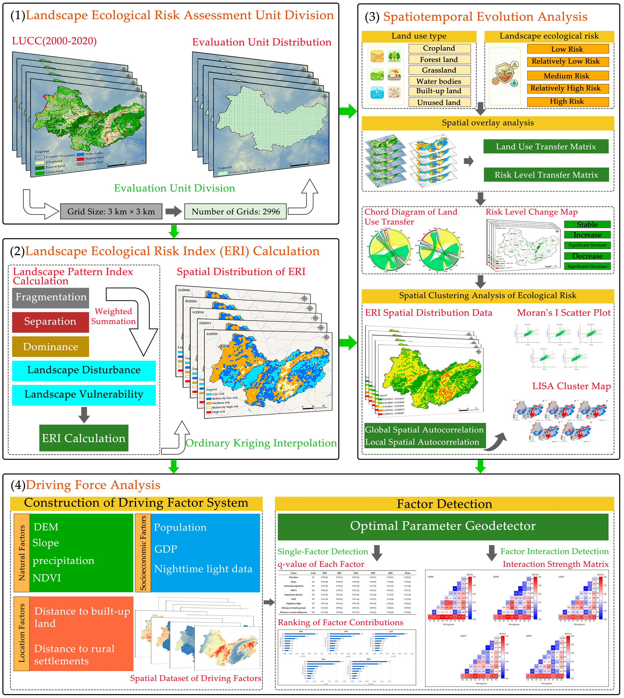
To provide a clear overview of the analytical workflow, we integrated the four methodological modules—evaluation unit division and land-use change analysis, landscape ecological risk assessment, spatial autocorrelation analysis, and geographical detector—into a unified technical framework (Figure 2). This framework illustrates the sequential processing of input data through each analytical step, culminating in the identification of spatiotemporal risk patterns and their driving factors.

3. Results

3.1. Spatiotemporal Changes in Land Use

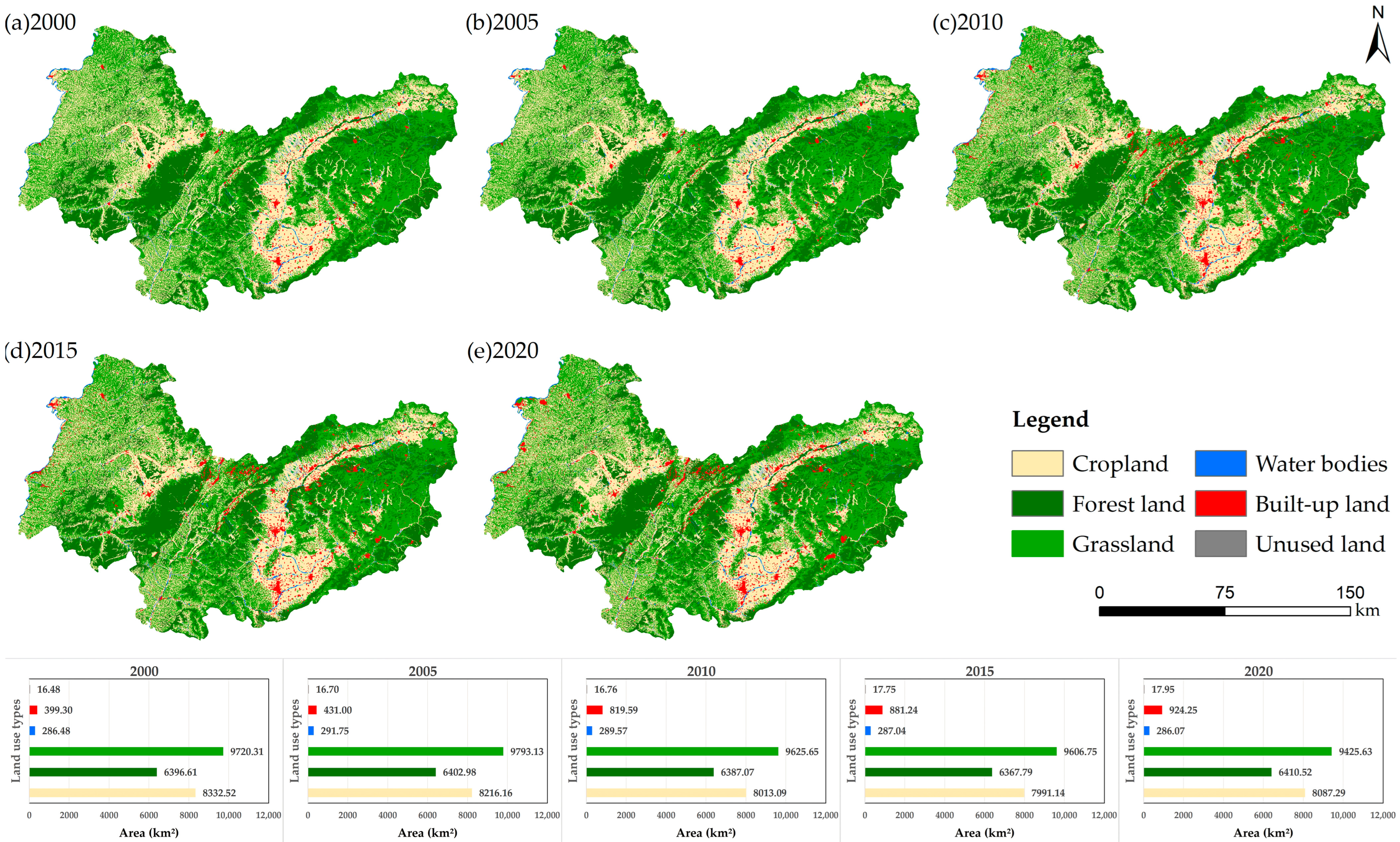
Over the 2000–2020 period, three land-use types—grassland, cropland, and forest land—consistently accounted for more than 95% of Xinzhou’s total area (Figure 3). Grassland was the most widespread cover, yet its extent gradually shrank from 9720.31 km² (38.65%) in 2000 to 9425.63 km² (37.48%) by 2020. Cropland followed a different trajectory: it first decreased from 8332.52 km² in 2000 to 7991.14 km² in 2015, then recovered slightly to 8087.29 km² in 2020. Forest land, in contrast, remained remarkably stable, gaining only 13.91 km² over the two decades—a negligible change. The most striking shift occurred in built-up land. Its area more than doubled, rising from 399.30 km² (1.59%) in 2000 to 924.25 km² (3.67%) in 2020, an increase of 131.47%. Water bodies and unused land categories showed little net change, either in area or percentage.

According to the land-use transfer matrix for the whole study period (

Table 3. Land use transfer matrix for Xinzhou City from 2000 to 2020 (unit: km²).

Land Use 2000	Land Use 2020						Total Out
	Cropland	Forest Land	Grassland	Water	Built-Up Land	Unused Land
Cropland	—	74.05	333.30	21.26	283.27	0.71	712.59
Forest land	74.23	—	113.86	4.13	70.38	1.30	263.90
Grassland	352.93	198.81	—	10.49	191.91	1.67	755.81
Water bodies	14.49	3.41	8.33	—	10.76	0.01	37.00
Built-up land	25.59	1.12	4.94	0.69	—	0.08	32.42
Unused land	0.25	0.19	0.55	0.01	1.31	—	2.31
Total in	467.48	277.58	460.98	36.57	557.64	3.77	1804.02

Note: The total area converted (sum of off-diagonal entries) is 1804.02 km². Row sums (“Total out”) and column sums (“Total in”) may differ slightly due to rounding; the values shown are as calculated from original data.

), about 1804.02 km² of land changed category. The dominant pattern was a back-and-forth conversion between cropland and grassland, with both types also losing substantial area to built-up land. Net outflows reached 294.68 km² for grassland and 245.23 km² for cropland, while built-up land gained 557.64 km² in net terms.

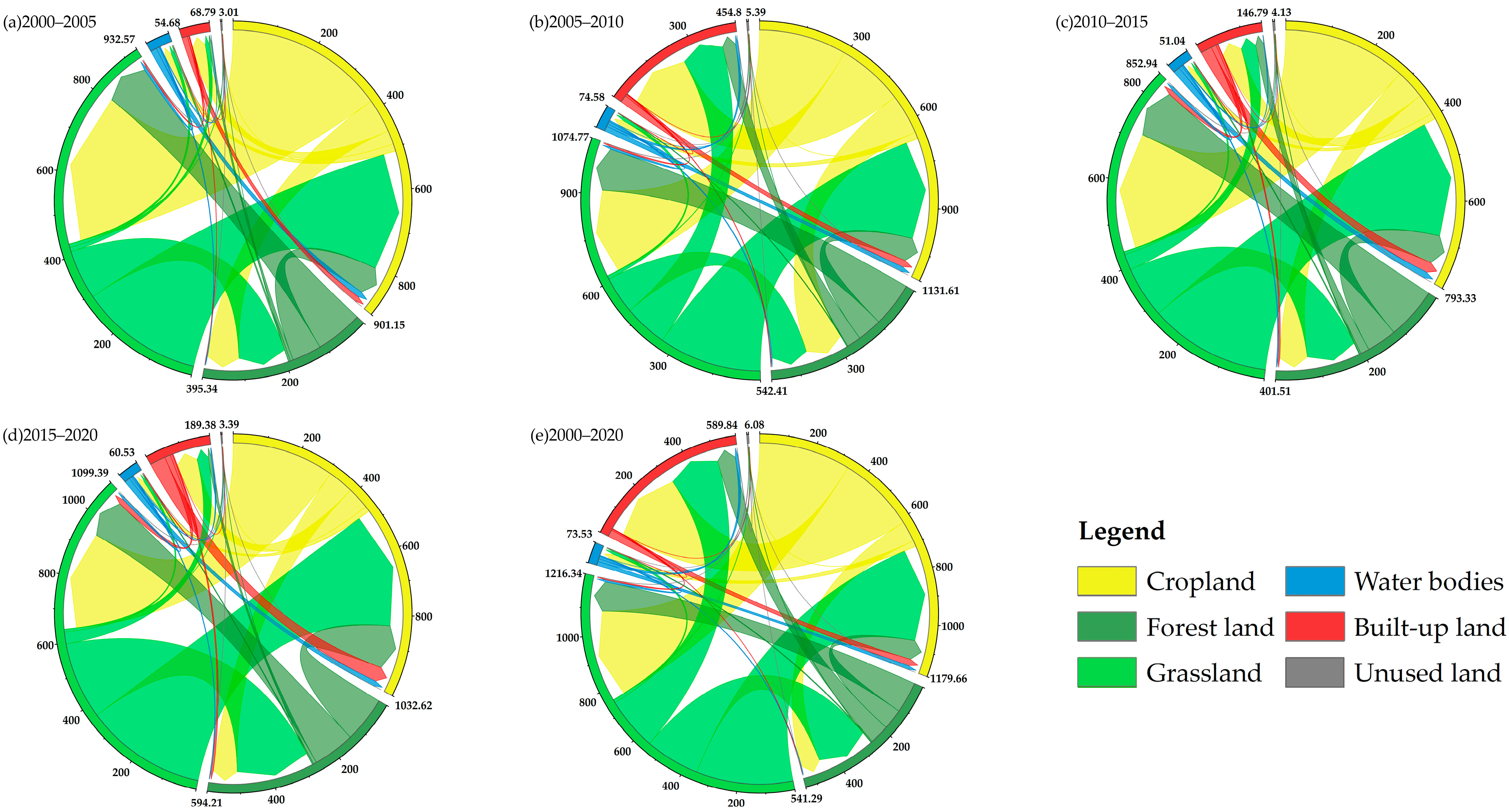
The dynamics varied considerably across the four sub-periods (Figure 4). Between 2000 and 2005, most cropland that was converted went to grassland (378.48 km²) or forest land (80.16 km²)—together representing over 80% of cropland outflows. Conversion of cropland to built-up land was still small, at just 32.77 km². During this period, cropland-to-grassland and cropland-to-forest conversions were predominant. At the same time, however, nearly 294 km² of grassland reverted to cropland, suggesting a coexistence of land abandonment and reclamation.

From 2005 to 2010, the picture changed. Cropland-to-built-up conversion increased substantially during this period. Grassland-to-cropland conversion also rose, to 341.44 km²—an indication that farming expansion may have been adding pressure alongside urban growth.

During 2010–2015, cropland outflows totaled 272.16 km² and grassland outflows 248.97 km², while built-up land expanded by 138.50 km². Interestingly, the sources of new urban land appeared to shift: instead of cropland, grassland began to contribute more. Exchanges between forest land and grassland remained active throughout.

In the final period (2015–2020), built-up land gained 153.87 km² from a wider variety of sources. Grassland-to-cropland conversion reached 364.34 km², the highest observed in any interval.

Taken together, these transitions show a clear temporal shift in land-use dynamics: ecological land expansion dominated before approximately 2005, followed by accelerated built-up land expansion afterward.

3.2. Spatiotemporal Evolution of Landscape Ecological Risk

3.2.1. Spatial and Temporal Distribution of Ecological Risk

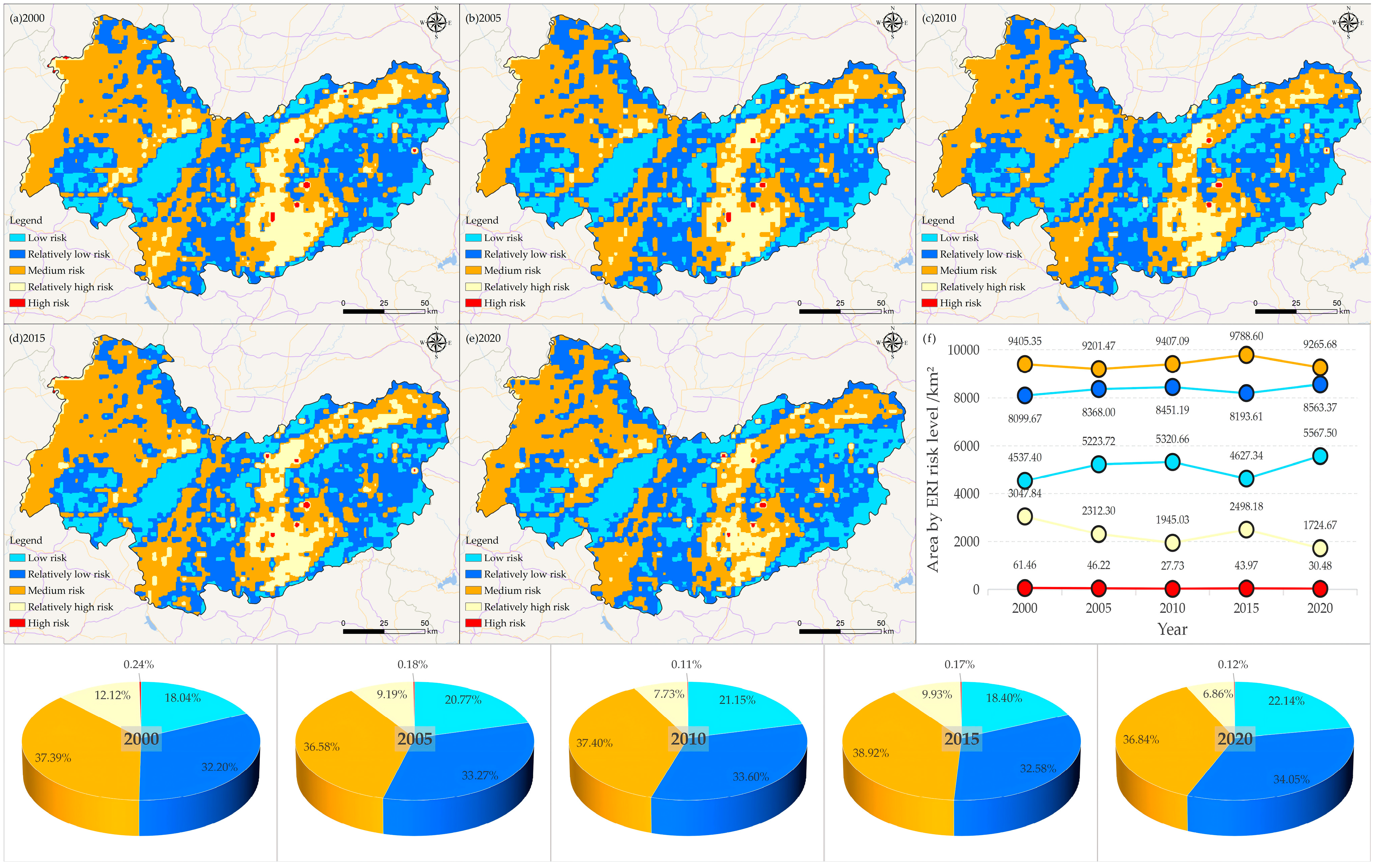
Spatial patterns. Risk distribution was strongly differentiated by land use (Figure 5a–e). Low-risk and relatively low-risk zones were concentrated in the western mountains (Ningwu, Yuanping, Kelan) and eastern Mount Wutai, where forest land and grassland cover remained continuous. The connectivity of these low-risk patches increased over time, forming the city’s core ecological source areas. Medium-risk zones, the most widespread class, displayed a mosaic pattern bridging the agricultural-forest-grassland transition zone in the western loess hills and encircling high-risk urban agglomerations in the east. Relatively high-risk zones clustered in intensively cultivated river valley basins (Xinfu District, Dingxiang County, Yuanping City) and mining areas (Dai County, Fanshi County). High-risk zones appeared as scattered small patches in urban cores, corresponding mainly to built-up land. Over the two decades, high-risk patches contracted in both number and size, yielding an overall spatial pattern of shrinking high-risk zones and expanding low-risk zones (Figure 5a–e).

Temporal dynamics. Between 2000 and 2020, landscape ecological risk in Xinzhou showed a clear improving trend (Figure 5f). The combined share of low-risk and relatively low-risk zones rose from 50.24% to 56.19%, with their area increasing from 4537.40 km² and 8099.67 km² to 5567.50 km² and 8563.37 km², respectively. The medium-risk zone remained the largest class throughout, fluctuating between 9200 and 9800 km² across the study periods. Relatively high-risk area fell by 43.41% (from 3047.84 km² to 1724.67 km²), and high-risk area dropped by 50.41% (from 61.46 km² to 30.48 km²). Together, the two highest risk levels contracted by 1354.15 km², suggesting a marked alleviation of regional ecological stress.

3.2.2. Transition of Ecological Risk Levels

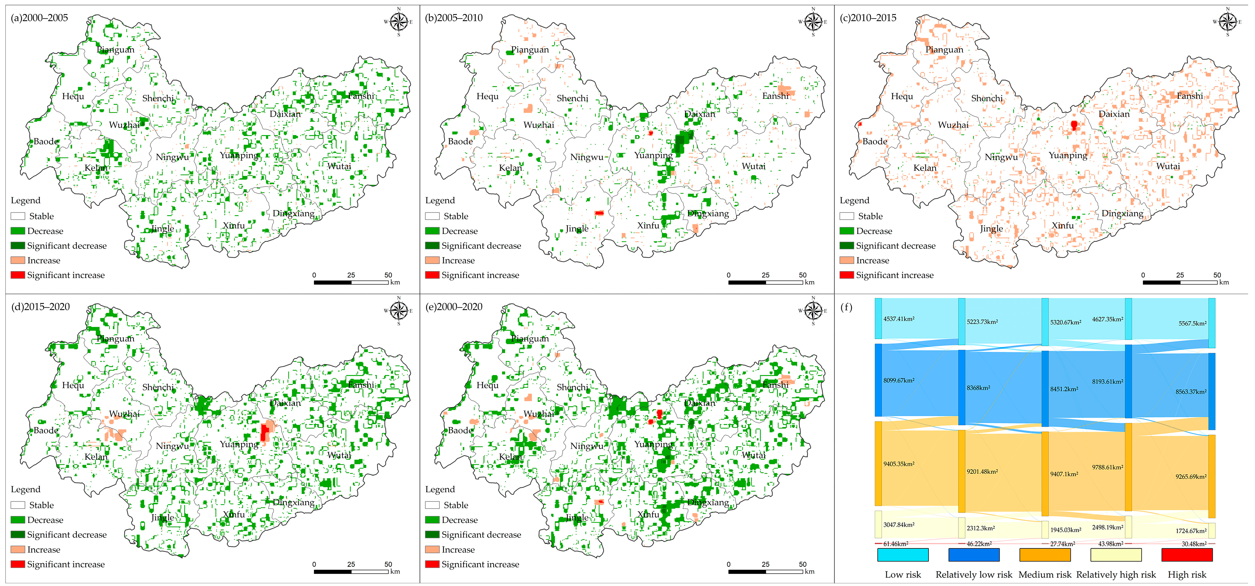
We tracked risk-level conversions by overlaying consecutive risk maps (Figure 6). Stable areas dominated throughout, comprising 85.71–93.79% of the landscape, suggesting that the baseline risk pattern persisted despite localized shifts.

Phase-specific patterns varied markedly across the four intervals (Figure 6a–d). During 2000–2005, 2508.92 km² (9.98%) transitioned to lower risk, concentrated in the western loess hills and eastern mountains; risk increase was minimal at 112.43 km² (0.45%). From 2005 to 2010, decreased-risk area shrank to 1077.57 km² (4.28%), while increased-risk area rose to 485.70 km² (1.93%) around urban centers such as Xinfu District and Yuanping City, reflecting early urbanization pressure. The 2010–2015 interval saw the sharpest deterioration: increased-risk area surged to 2274.07 km² (9.04%), the highest of any period. In contrast, 2015–2020 showed the strongest recovery, with decreased-risk area reaching 3332.91 km² (13.25%) and increased-risk area falling to 216.11 km² (0.86%). Cross-level jumps (changes of two or more levels) remained below 0.25% in each interval, suggesting that conversions occurred mainly between adjacent levels.

Over the full 20-year span (Figure 6e), the spatial pattern of risk transition reflected the cumulative effect of these phased shifts. The alluvial diagram (Figure 6f) further quantifies the area exchanged among risk levels over time: low-risk and relatively low-risk zones expanded mainly through risk reduction from medium-risk zones, whereas medium-risk zones lost area to relatively high-risk zones during 2010–2015 before regaining it during 2015–2020. High-risk zones remained largely isolated, with minimal two-way exchange, underscoring their tight coupling with built-up land.

3.3. Spatial Clustering Characteristics of Ecological Risk

3.3.1. Global Spatial Autocorrelation

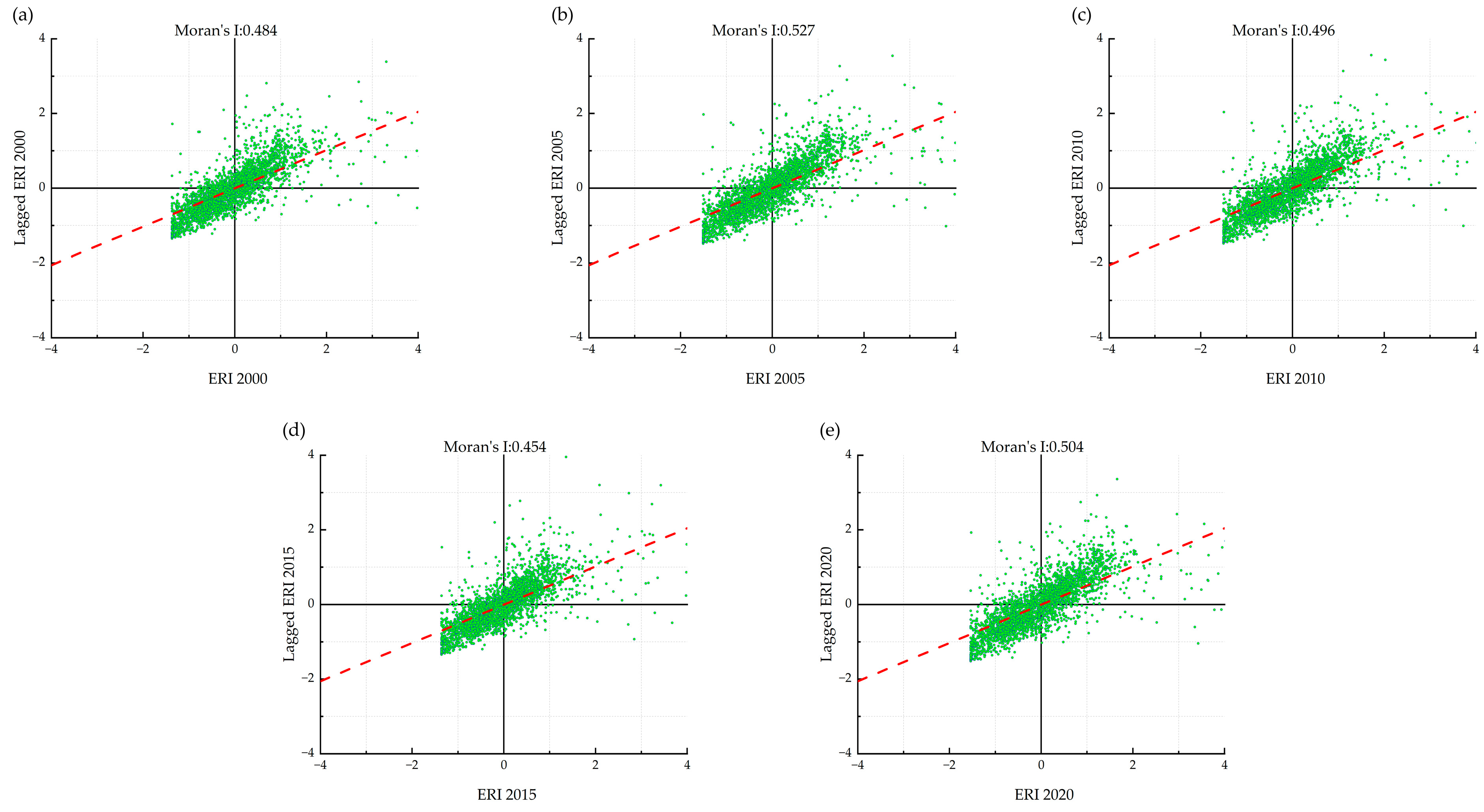
Global Moran’s I values for the five periods were 0.484, 0.527, 0.496, 0.454, and 0.504, respectively (Figure 7). All values were positive and significant at p < 0.01, confirming consistently strong positive spatial autocorrelation in landscape ecological risk—units with similar risk levels tended to cluster spatially.

The temporal trajectory of Moran’s I followed a rise–fall–rise pattern (Figure 7a–e). The index increased from 0.484 in 2000 to a peak of 0.527 in 2005 (Figure 7a,b), suggesting that the contiguous expansion of risk-reduced zones strengthened overall spatial clustering. From 2005 to 2015, Moran’s I declined to 0.454 (Figure 7b–d), reflecting weakened global clustering as risk increases became scattered across multiple locations rather than concentrated. The index then rose to 0.504 by 2020 (Figure 7e).

3.3.2. Local Spatial Autocorrelation

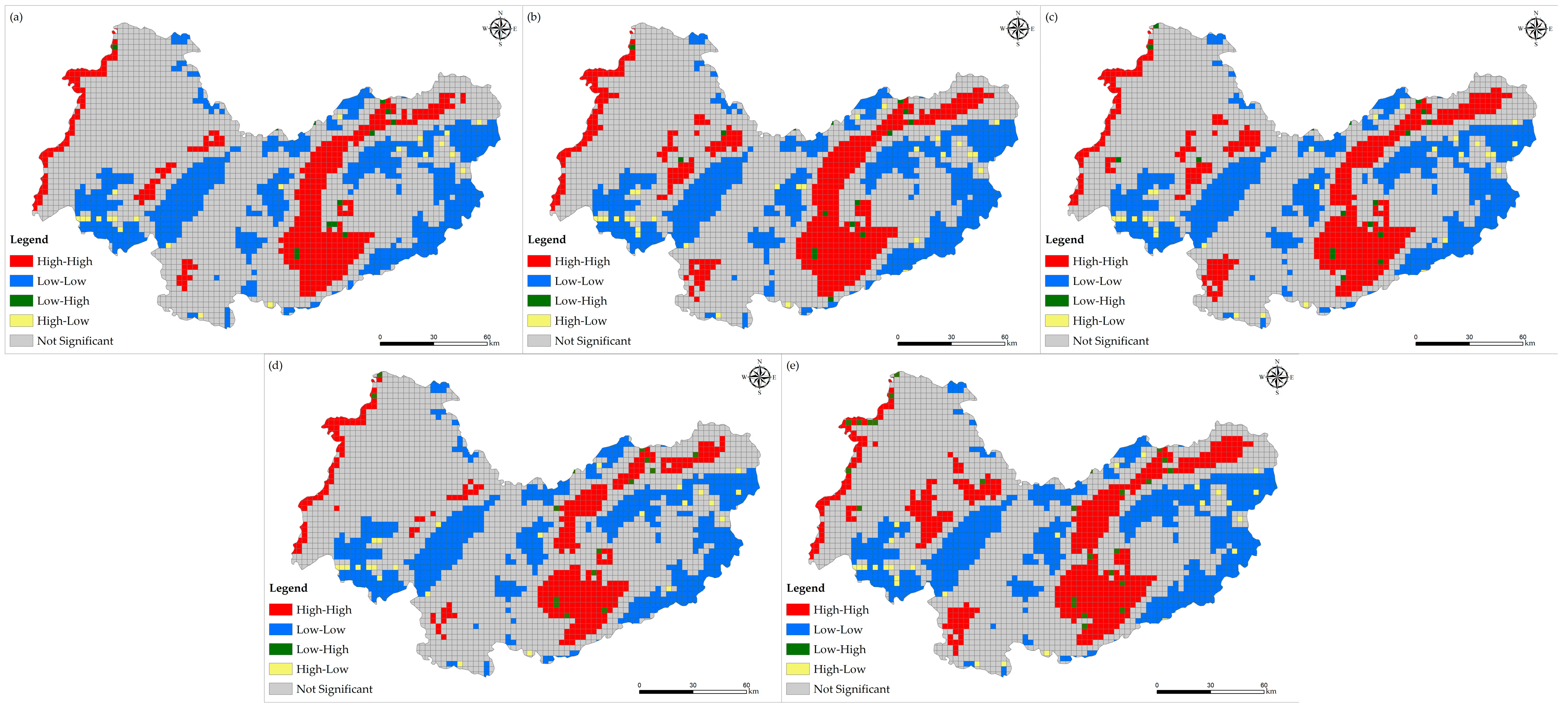
Local Moran’s I analysis identified four cluster types: high–high (HH), low–low (LL), high–low (HL), and low–high (LH) (Figure 8).

LL clusters occupied the western Guancen–Luya Mountains and eastern Mount Wutai areas across all periods (Figure 8). These high-elevation, well-vegetated forest and grassland zones with limited human activity functioned as stable ecological source areas. HH clusters were concentrated in the Xinding Basin and river valleys, where intensive cropland and moderate vulnerability sustained persistent risk hotspots.

Temporal dynamics showed clear phase shifts (Figure 8a–e). From 2000 to 2005, LL clusters expanded while HH clusters contracted (Figure 8a,b), reflecting the expansion of low-risk zones in mountainous areas. From 2005 to 2010, LL clusters shrank and HH patches emerged around Xinfu District and Yuanping City (Figure 8b,c), consistent with urbanization-induced risk concentration. During 2010–2015, both LL and HH clusters contracted markedly; many former HH areas became non-significant (Figure 8c,d), consistent with the scattered risk increases noted in Section 3.2.2. From 2015 to 2020, LL clusters regained their earlier extent while HH clusters remained suppressed (Figure 8d,e), suggesting that vegetation recovery in these areas re-established the core-periphery risk pattern.

HL and LH outliers remained sporadic throughout, each accounting for less than 1% of total units in all periods.

3.4. Driving Factors of Landscape Ecological Risk Evolution

3.4.1. Single-Factor Detection

We quantified the explanatory power of nine driving factors using the optimal-parameter geographical detector (

Table 4. Explanatory power (q-values) of single driving factors for landscape ecological risk in Xinzhou City, 2000–2020.

Factor	Code	2000	2005	2010	2015	2020	Mean
Elevation	X1	0.32 (1)	0.30 (1)	0.28 (1)	0.29 (1)	0.30 (1)	0.30 (1)
Slope	X2	0.06 (8)	0.05 (7)	0.05 (8)	0.05 (8)	0.05 (8)	0.05 (8)
Annual precipitation	X3	0.17 (2)	0.19 (2)	0.18 (2)	0.17 (3)	0.12 (5)	0.17 (2)
NDVI	X4	0.14 (6)	0.13 (5)	0.11 (6)	0.10 (6)	0.06 (7)	0.11 (6)
Population density	X5	0.16 (3)	0.16 (3)	0.14 (5)	0.13 (4)	0.13 (3)	0.14 (4)
GDP	X6	0.15 (4)	0.04 (8)	0.16 (4)	0.13 (5)	0.13 (4)	0.12 (5)
Nighttime light	X7	0.01 (9)	0.01 (9)	0.01 (9)	0.01 (9)	0.02 (9)	0.01 (9)
Distance to built-up land	X8	0.10 (7)	0.09 (6)	0.09 (7)	0.09 (7)	0.08 (6)	0.09 (7)
Distance to rural settlements	X9	0.15 (5)	0.13 (4)	0.17 (3)	0.18 (2)	0.18 (2)	0.16 (3)

Note: X1, elevation; X2, slope; X3, annual precipitation; X4, NDVI; X5, population density; X6, GDP; X7, nighttime light; X8, distance to built-up land; X9, distance to rural settlements. Values in parentheses are rankings based on q-values for each year. The mean q-value is averaged across the five periods.

). Natural factors dominated the spatial differentiation of landscape ecological risk throughout the study period. Elevation (X1) consistently ranked first, with q-values ranging from 0.28 to 0.32 (mean 0.30), reflecting the steep topographic gradient that shapes land use intensity and human activity distribution. Annual precipitation (X3) ranked second (mean q = 0.17), while NDVI (X4) declined from 0.14 in 2000 to 0.06 in 2020, possibly reflecting vegetation cover homogenization associated with ecological restoration. Among socioeconomic factors, population density (X5) and GDP (X6) showed similar but declining explanatory power (mean q = 0.14 and 0.12, respectively), consistent with a weakening spatial coupling between human activities and risk patterns as ecological protection intensified. Notably, the explanatory power of distance to rural settlements (X9) increased from 0.15 in 2000 to 0.18 in 2020 (mean q = 0.16), suggesting a growing spatial association between rural settlement proximity and risk patterns, whereas that of distance to built-up land (X8) remained low and stable (mean q = 0.09). Slope (X2) and nighttime light intensity (X7) had weak to negligible effects throughout (q ≈ 0.05 and 0.01, respectively).

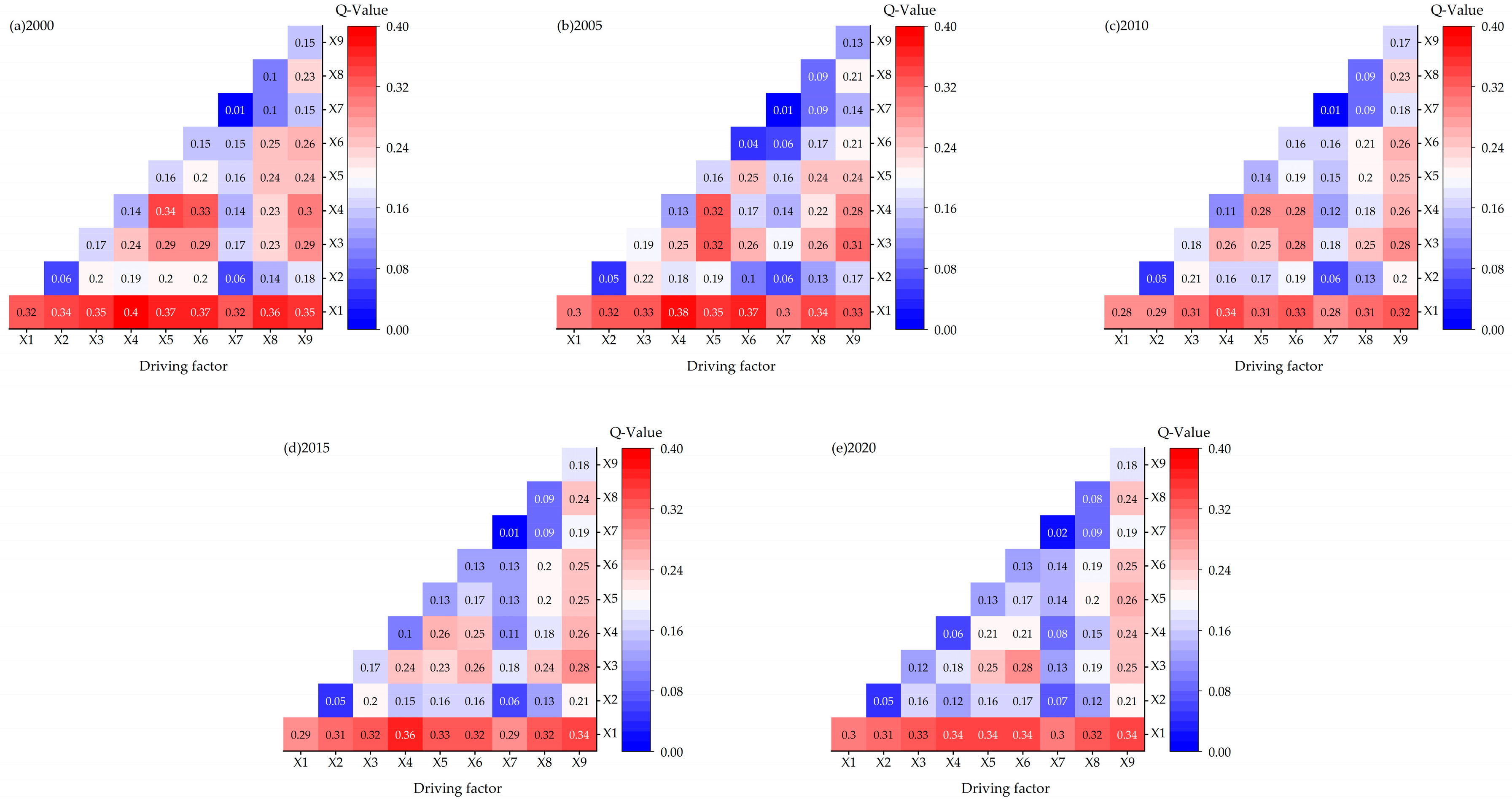
3.4.2. Factor Interaction Detection

Most factor pairs showed bivariate or non-linear enhancement (Figure 9), suggesting that risk spatial differentiation is driven by combined synergistic effects in addition to single-factor influences. Interactions involving elevation (X1) were the core drivers. Elevation ∩ NDVI (X1 ∩ X4) consistently yielded the highest q-values (0.34–0.40), reflecting that elevation governs vertical temperature and moisture gradients, which directly determine vegetation cover patterns and thus shape risk heterogeneity. Elevation ∩ population (X1 ∩ X5) and elevation ∩ GDP (X1 ∩ X6) maintained q-values of 0.30–0.37, confirming that elevation constrains not only natural landscapes but also the spatial distribution of population and economic activity—a coupling between terrain constraints and human responses. Interactions among purely natural factors (X1 ∩ X2, X1 ∩ X3, X2 ∩ X4) were moderately strong and stable, constituting the fundamental environmental framework. In contrast, interactions among socioeconomic and location factors (X5 ∩ X6, X5 ∩ X7, X8 ∩ X9) had weak explanatory power, suggesting that human activities have limited independent explanatory power for spatial risk differentiation and require coupling with terrain, vegetation, or other natural conditions to shape spatial patterns. Overall, the driving mechanism in Xinzhou is characterized by natural factors exerting primary control, with anthropogenic factors playing a secondary, modulatory role.

4. Discussion

Our results reveal three salient patterns in Xinzhou’s landscape ecological risk dynamics from 2000 to 2020. First, overall risk declined, with high- and relatively high-risk zones shrinking by more than 1350 km². Second, this decline was nonlinear: risk intensified between 2005 and 2015 when urbanization and mining expansion peaked [41,42], then recovered after 2015. Third, the spatial pattern remained stable throughout—higher risk in basins, lower risk in mountains—reflecting persistent topographic control over land-use intensity [43]. These findings extend earlier landscape ecological risk assessments in the Loess Plateau [44,45,46] by demonstrating that cities in ecologically sensitive transition zones exhibit distinct policy-driven fluctuations shaped by the interplay of resource extraction, agricultural intensification, and urban expansion. While previous studies have documented risk patterns in the Yellow River Basin [47,48], most of them relied on static or short-term analyses that cannot capture the temporal coupling between policy interventions, urbanization pulses, and ecological restoration. Our 20-year analysis identifies a clear three-stage trajectory—policy-driven improvement (2000–2005), urbanization-aggravated deterioration (2005–2015), and restoration-led recovery (2015–2020)—which aligns closely with regional policy shifts and mining activity cycles. While annual precipitation showed moderate explanatory power (mean q = 0.17, Table 4), its ranking remained stable across periods and did not exhibit the phase-specific shifts characteristic of policy-driven variables. This suggests that climate variability, though contributing to baseline risk heterogeneity, was not the primary driver of the observed temporal trajectory. This temporal specificity is critical for understanding why risk trends in ecologically sensitive transition zones cannot be inferred from single-period assessments.

Specifically, the early improvement (2000–2005) aligned with the Grain-for-Green program. Risk reduction was largest (2508.92 km²) and concentrated in the western loess hills and eastern mountains, where steep cropland conversion was most extensive. This pattern supports national reforestation benefits and adds spatial detail [49]. The subsequent deterioration (2005–2015) presents a more complex picture: unlike typical urbanization narratives where built-up expansion dominates risk increases, Xinzhou’s surge was amplified by coal mining intensification [50], a driver poorly captured by nighttime light data. This explains the negligible explanatory power of X7 (q ≈ 0.01) and underscores that standard socioeconomic proxies may fail to represent dispersed, subterranean resource extraction [51,52]. The recovery phase (2015–2020) reflects compounding effects of a new Grain-for-Green round and enhanced mine rehabilitation, suggesting that ecological investments in mixed land-use cities can achieve measurable risk reductions within 5-year policy cycles. The weak explanatory power of slope (X2, q ≈ 0.05) may seem counterintuitive given the steep terrain of the Loess Plateau. In Xinzhou’s rugged topography, elevation integrates vertical position, temperature gradients, moisture regimes, and vegetation zonation, making it a more comprehensive proxy for the physical controls on ecological risk. Slope influences erosion primarily through its role in empirical frameworks such as the RUSLE, although this effect is strongly moderated by vegetation cover and terracing [53,54]. Moreover, slope operates at finer scales—such as within-field soil erosion—that are not resolvable at the 3 km grid resolution, whereas elevation captures the broader topographic control structuring landscape patterns at the assessment scale. The limited independent contribution of slope thus reflects a combination of scale mismatch and vegetation-mediated attenuation, rather than statistical redundancy with elevation. This interpretation aligns with Yan et al. [55], who reported similar elevation-dominant patterns in the Yellow River Basin when both variables were included in geographical detector models.

The persistent “basin-high, mountain-low” risk pattern reflects a cascading control where elevation shapes temperature and moisture gradients that determine vegetation cover and modulate landscape vulnerability—explaining why X1 maintained dominant explanatory power (q = 0.28–0.32) and X1∩X4 produced the strongest interaction effects (q = 0.34–0.40) throughout the study period. This top-down control aligns with findings from the broader Loess Plateau [56], yet the growing explanatory power of distance to rural settlements (X9: 0.15 → 0.18) suggests progressive human penetration into this natural framework, particularly in agricultural-forest-grassland transition zones—a pattern consistent with the edge effect of rural settlement expansion observed in northern China’s mountainous regions [57]. The HH clusters in the Xinding Basin represent a structurally embedded risk where intensive cropland is both economically essential and ecologically vulnerable, a tension documented similarly in the Weihe River Basin and Guanzhong Plain [58,59]. Rather than eliminating this risk, management should buffer it by maintaining LL clusters in the Guancen-Luya Mountains and Mount Wutai as ecological source areas while improving agricultural practices in the basin—aligning with the “ecological security pattern” concept of differentially managing source areas and buffer zones to optimize conservation and production goals [60].

Our interaction results help clarify how humans and land interact in mountain–basin systems. Natural–natural interactions stayed strong and stable, whereas socioeconomic-socioeconomic interactions remained weak unless combined with natural factors. This contrast suggests that in rugged terrain, human disturbance is “spatially compressed” into low-elevation suitable zones, not spread evenly. These findings fit our proposed “terrain-constrained human-land coupling framework”, which extends territorial system theory [61] by treating elevation as a structural force, not just a background variable. The finding that X1∩X5 and X1∩X6 (elevation ∩ population/GDP) maintained high explanatory power (0.30–0.37) confirms that population and economic activity are not randomly distributed but topographically channeled. This has methodological implications: future studies should incorporate topographic constraints into spatial interaction models rather than treating human and natural drivers as additive layers [62,63]. Furthermore, the declining explanatory power of population density and GDP over time (Table 4) suggests that ecological protection policies have partially weakened the spatial association between economic growth from risk increases—indicative of a potential dissociation trajectory for sustainable development in resource regions.

We also note that built-up land emerges as a high-risk component despite its low vulnerability ranking, reflecting an inherent feature of the composite ERI framework: vulnerability and disturbance interact through area-weighting. This does not compromise the validity of the trend analysis but suggests that future work could benefit from decomposing the ERI into vulnerability-driven and disturbance-driven components. Four limitations warrant acknowledgment. First, no spatially explicit mining intensity variable was included, despite the study area’s status as a major coal-producing region; publicly available data at the required temporal resolution were lacking, though the observed risk deterioration phase (2010–2015) coincided with documented mining peaks in Shanxi Province. Second, the landscape vulnerability index relies on expert-assigned weights, introducing potential subjectivity. Third, the spatial quantification of policy variables (e.g., reforestation subsidies, mining quotas) was not feasible. Fourth, the 3 km grid resolution, though appropriate for meso-scale analysis, may mask fine-scale heterogeneity operating at sub-kilometer scales [35].

Notwithstanding these limitations, the findings carry management implications: risk prevention merits prioritization in rural settlement peripheries and urban expansion zones characterized by dynamic human–land coupling, whereas precision agriculture and ecological compensation may alleviate agriculture-related ecological risks in the Xinding Basin. These spatially explicit risk maps can further inform climate adaptation planning: the low-risk mountain areas (Guancen-Luya Mountains, Mount Wutai) represent priority zones for maintaining ecological connectivity and restricting land-use conversion, while the high-risk basin areas require integrated strategies combining climate-resilient agricultural practices and green infrastructure to buffer against urbanization and climatic variability. These strategies align with SDG 15.1 (conservation of mountain ecosystems), SDG 11.a (urban-rural linkages), and SDG 15.9 (integration of ecosystem values into planning)—the latter evidenced by the weakening spatial association between economic growth and ecological risk (declining q-values for GDP and population density, Table 4).

Future research should advance along three complementary tracks. First, methodological refinement: decomposing the ERI into vulnerability-driven and disturbance-driven components would evaluate the sources of risk and clarify the built-up land anomaly, while multi-scale nested grids and systematic sensitivity analysis would evaluate the robustness of findings under alternative scales and weighting schemes. Second, data enrichment: remote sensing-derived mining disturbance indices should be developed to capture subterranean extraction impacts, governance variables—including land-use planning zones, ecological compensation boundaries, and mining concessions—should be spatialized to enable direct testing of policy effects, and post-2020 land-use and auxiliary data should be incorporated once available to validate the observed long-term trends. Third, scenario projection: once governance variables are spatialized, InVEST ecosystem service valuation [64] and FLUS/PLUS scenario modeling [65] could be integrated to project risk trajectories under alternative policy regimes.

5. Conclusions

This study examined the spatiotemporal dynamics of landscape ecological risk and its driving mechanisms in Xinzhou City, a typical ecologically sensitive transition zone in the middle Yellow River Basin, using land-use data from five time points between 2000 and 2020. Over this period, overall risk levels declined, with high- and relatively high-risk zones contracting by 1354.15 km². This improvement was not linear—alternating phases of reduction and increase across sub-periods suggest a trajectory shaped by the interplay of ecological interventions and anthropogenic pressures. Spatially, the risk distribution remained stable, characterized by elevated risk in basin areas and reduced risk in mountainous zones. Low–low clusters were consistently concentrated in the Guancen–Luya Mountains and Mount Wutai, while high–high clusters persisted in the Xinding Basin. Elevation emerged as the dominant factor explaining spatial risk differentiation (q = 0.28–0.32), and the explanatory power of distance to rural settlements increased from 0.15 to 0.18 over the study period. Elevation and NDVI together consistently exerted the strongest joint influence on risk patterns (q = 0.34–0.40).

These findings underscore the need for spatially differentiated risk management in mountain–basin systems, with priority given to conserving ecological source areas and regulating disturbance-prone zones—particularly rural peripheries and expanding urban fringes. By linking ecological risk assessment to place-based interventions, this study provides actionable insights relevant to SDG 15 (Life on Land) and SDG 11 (Sustainable Cities and Communities).

References

1. Wang, H.; Liu, X.; Zhao, C.; Chang, Y.; Liu, Y.; Zang, F. Spatial-temporal pattern analysis of landscape ecological risk assessment based on land use/land cover change in Baishuijiang National nature reserve in Gansu Province, China. Ecol. Indic. 2021, 124, 107454. [Google Scholar] [CrossRef] [Scilit]
2. Gao, H.; Song, W. Assessing the landscape ecological risks of land-use change. Int. J. Environ. Res. Public Health 2022, 19, 13945. [Google Scholar] [CrossRef] [Scilit] [PubMed]
3. Qian, Y.; Dong, Z.; Yan, Y.; Tang, L. Ecological risk assessment models for simulating impacts of land use and landscape pattern on ecosystem services. Sci. Total Environ. 2022, 833, 155218. [Google Scholar] [CrossRef] [Scilit] [PubMed]
4. Du, L.; Dong, C.; Kang, X.; Qian, X.; Gu, L. Spatiotemporal evolution of land cover changes and landscape ecological risk assessment in the Yellow River Basin, 2015–2020. J. Environ. Manag. 2023, 332, 117149. [Google Scholar] [CrossRef] [Scilit] [PubMed]
5. Yang, Y.; Chen, J.; Lan, Y.; Zhou, G.; You, H.; Han, X.; Wang, Y.; Shi, X. Landscape pattern and ecological risk assessment in Guangxi based on land use change. Int. J. Environ. Res. Public Health 2022, 19, 1595. [Google Scholar] [CrossRef] [Scilit] [PubMed]
6. Karimian, H.; Zou, W.; Chen, Y.; Xia, J.; Wang, Z. Landscape ecological risk assessment and driving factor analysis in Dongjiang river watershed. Chemosphere 2022, 307, 135835. [Google Scholar] [CrossRef] [Scilit] [PubMed]
7. Yang, N.; Zhang, T.; Li, J.; Feng, P.; Yang, N. Landscape ecological risk assessment and driving factors analysis based on optimal spatial scales in Luan River Basin, China. Ecol. Indic. 2024, 169, 112821. [Google Scholar] [CrossRef] [Scilit]
8. Ren, D.; Cao, A. Analysis of the heterogeneity of landscape risk evolution and driving factors based on a combined GeoDa and Geodetector model. Ecol. Indic. 2022, 144, 109568. [Google Scholar] [CrossRef] [Scilit]
9. Li, X.; Li, S.; Zhang, Y.; O’Connor, P.J.; Zhang, L.; Yan, J. Landscape ecological risk assessment under multiple indicators. Land 2021, 10, 739. [Google Scholar] [CrossRef] [Scilit]
10. Wang, S.; Tan, X.; Fan, F. Landscape ecological risk assessment and impact factor analysis of the Qinghai–Tibetan Plateau. Remote Sens. 2022, 14, 4726. [Google Scholar] [CrossRef] [Scilit]
11. Lan, Y.; Chen, J.; Yang, Y.; Ling, M.; You, H.; Han, X. Landscape pattern and ecological risk assessment in Guilin based on land use change. Int. J. Environ. Res. Public Health 2023, 20, 2045. [Google Scholar] [CrossRef] [Scilit] [PubMed]
12. Qu, Y.; Zong, H.; Su, D.; Ping, Z.; Guan, M. Land use change and its impact on landscape ecological risk in typical areas of the Yellow River Basin in China. Int. J. Environ. Res. Public Health 2021, 18, 11301. [Google Scholar] [CrossRef] [Scilit] [PubMed]
13. Li, M.; Abuduwaili, J.; Liu, W.; Feng, S.; Saparov, G.; Ma, L. Application of geographical detector and geographically weighted regression for assessing landscape ecological risk in the Irtysh River Basin, Central Asia. Ecol. Indic. 2024, 158, 111540. [Google Scholar] [CrossRef] [Scilit]
14. Yan, Z.; Wang, Y.; Wang, Z.; Zhang, C.; Wang, Y.; Li, Y. Spatiotemporal analysis of landscape ecological risk and driving factors: A case study in the Three Gorges Reservoir Area, China. Remote Sens. 2023, 15, 4884. [Google Scholar] [CrossRef] [Scilit]
15. Shamuxi, A.; Han, B.; Jin, X.; Wusimanjiang, P.; Abudukerimu, A.; Chen, Q.; Zhou, H.; Gong, M. Spatial pattern and driving mechanisms of dryland landscape ecological risk: Insights from an integrated geographic detector and machine learning model. Ecol. Indic. 2025, 172, 113305. [Google Scholar] [CrossRef] [Scilit]
16. Wang, Q.; Zhang, P.; Chang, Y.; Li, G.; Chen, Z.; Zhang, X.; Xing, G.; Lu, R.; Li, M.; Zhou, Z. Landscape pattern evolution and ecological risk assessment of the Yellow River Basin based on optimal scale. Ecol. Indic. 2024, 158, 111381. [Google Scholar] [CrossRef] [Scilit]
17. Tan, R.; Zhou, K. Examining the causal effects of road networks on landscape ecological risk: The case of Wuhan, China. J. Urban Plan. Dev. 2023, 149, 05023004. [Google Scholar] [CrossRef] [Scilit]
18. Chen, H.; Chen, H.; Huang, X.; Zhang, S.; He, T.; Gao, Z. Landscape ecological risk assessment and driving factor analysis in southwest China. Sci. Rep. 2024, 14, 23208. [Google Scholar] [CrossRef] [Scilit] [PubMed]
19. Xu, W.; Yao, W.; Wang, H.; Yang, J.; Yu, T.; Yu, H. Assessing landscape ecological risk from mining in the river source region of the Yellow River Basin. Land 2025, 14, 2152. [Google Scholar] [CrossRef] [Scilit]
20. Zhu, Z.; Mei, Z.; Xu, X.; Feng, Y.; Ren, G. Landscape ecological risk assessment based on land use change in the Yellow River Basin of Shaanxi, China. Int. J. Environ. Res. Public Health 2022, 19, 9547. [Google Scholar] [CrossRef] [Scilit] [PubMed]
21. Li, J.; Li, S.; Wang, X.; Xu, G.; Pang, J. Spatio-temporal variations and multi-scenario simulation of landscape ecological risk in the drylands of the Yellow River Basin. Sci. Rep. 2024, 14, 22672. [Google Scholar] [CrossRef] [Scilit] [PubMed]
22. Yu, L.; Zhou, J.; Wang, J.; Xu, H.; Li, Y.; Chen, F.; Liu, Y. Spatiotemporal evolution and driving forces of landscape ecological risk in the lower reaches of the Yellow River from 2000 to 2020. Sci. Rep. 2025, 15, 21375. [Google Scholar] [CrossRef] [Scilit] [PubMed]
23. Li, H.; Sun, H.; Sun, S.; Wang, S. Spatiotemporal non-stationarity and driving mechanisms of ecological risk in the Three Gorges Reservoir Area: Integrating land use patterns and terrain positioning into multi-scale geospatial modeling. Land Degrad. Dev. 2025, 37, 3483–3500. [Google Scholar] [CrossRef] [Scilit]
24. Li, F.; Tian, N.; Zhang, H.; Luo, K.; Xiang, K.; Peng, Y. Evaluating ecological vulnerability and its driving mechanisms in the Dongting Lake Region from a multi-method integrated perspective: Based on Geodetector and explainable machine learning. Land 2025, 14, 1435. [Google Scholar] [CrossRef] [Scilit]
25. Qiao, F.; Bai, Y.; Xie, L.; Yang, X.; Sun, S. Spatio-temporal characteristics of landscape ecological risks in the ecological functional zone of the Upper Yellow River, China. Int. J. Environ. Res. Public Health 2021, 18, 12943. [Google Scholar] [CrossRef] [Scilit] [PubMed]
26. Chang, S.; Dai, Z.; Wang, X.; Zhu, Z.; Feng, Y. Landscape pattern identification and ecological risk assessment employing land use dynamics on the Loess Plateau. Agronomy 2023, 13, 2247. [Google Scholar] [CrossRef] [Scilit]
27. Ren, Y.; Lü, Y.; Fu, B.; Comber, A.; Li, T.; Hu, J. Driving factors of land change in China’s Loess Plateau: Quantification using geographically weighted regression and management implications. Remote Sens. 2020, 12, 453. [Google Scholar] [CrossRef] [Scilit]
28. Zhang, H.; Zhang, J.; Lv, Z.; Yao, L.; Zhang, N.; Zhang, Q. Spatio-temporal assessment of landscape ecological risk and associated drivers: A case study of the Yellow River Basin in Inner Mongolia. Land 2023, 12, 1114. [Google Scholar] [CrossRef] [Scilit]
29. Dong, Y.; Yin, D.; Li, X.; Huang, J.; Su, W.; Li, X.; Wang, H. Spatial–temporal evolution of vegetation NDVI in association with climatic, environmental and anthropogenic factors in the Loess Plateau, China during 2000–2015: Quantitative analysis based on geographical detector model. Remote Sens. 2021, 13, 4380. [Google Scholar] [CrossRef] [Scilit]
30. Wang, W.; Xue, X.; Wang, Z.; Zhang, Q. Multiscale driving mechanisms and spatial non-stationarity of landscape ecological risk based on an OPGD–MGWR framework: Evidence from township-level units in the Nanjing metropolitan area (NMA), China. Ecol. Indic. 2026, 186, 114840. [Google Scholar] [CrossRef] [Scilit]
31. Tian, L.; Yang, F.; Huang, D.; Luo, Y.; Wu, Y.; Wen, C. Land-use transformation and landscape ecological risk assessment in the Three Gorges Reservoir Region based on the “Production–Living–Ecological Space” perspective. Land 2022, 11, 1234. [Google Scholar] [CrossRef] [Scilit]
32. Peng, J.; Zong, M.; Hu, Y.; Liu, Y.; Wu, J. Assessing landscape ecological risk in a mining city: A case study in Liaoyuan City, China. Sustainability 2015, 7, 8312–8334. [Google Scholar] [CrossRef] [Scilit]
33. Zhang, X.; Du, H.; Wang, Y.; Chen, Y.; Ma, L.; Dong, T. Watershed landscape ecological risk assessment and landscape pattern optimization: Take Fujiang River Basin as an example. Hum. Ecol. Risk Assess. 2021, 27, 2254–2276. [Google Scholar] [CrossRef] [Scilit]
34. Zhang, M.; Kafy, A.; Ren, B.; Zhang, Y.; Tan, S.; Li, J. Application of the optimal parameter geographic detector model in the identification of influencing factors of ecological quality in Guangzhou, China. Land 2022, 11, 1303. [Google Scholar] [CrossRef] [Scilit]
35. Liu, Y.; Liu, Y.; Li, J.; Lu, W.; Wei, X.; Sun, C. Evolution of landscape ecological risk at the optimal scale: A case study of the open coastal wetlands in Jiangsu, China. Int. J. Environ. Res. Public Health 2018, 15, 1691. [Google Scholar] [CrossRef] [Scilit] [PubMed]
36. Chen, Z.; Feng, H.; Liu, X.; Wang, H.; Hao, C. Analysis of the influence of driving factors on vegetation changes based on the optimal-parameter-based geographical detector model in the Yima Mining Area. Forests 2024, 15, 1573. [Google Scholar] [CrossRef] [Scilit]
37. Li, S.; Tu, B.; Zhang, Z.; Wang, L.; Zhang, Z.; Che, X.; Wang, Z. Exploring new methods for assessing landscape ecological risk in key basin. J. Clean. Prod. 2024, 461, 142633. [Google Scholar] [CrossRef] [Scilit]
38. Sun, N.; Chen, Q.; Liu, F.; Zhou, Q.; He, W.; Guo, Y. Land use simulation and landscape ecological risk assessment on the Qinghai-Tibet Plateau. Land 2023, 12, 923. [Google Scholar] [CrossRef] [Scilit]
39. Lin, X.; Wang, Z. Landscape ecological risk assessment and its driving factors of multi-mountainous city. Ecol. Indic. 2023, 146, 109823. [Google Scholar] [CrossRef] [Scilit]
40. Li, S.; He, W.; Wang, L.; Zhang, Z.; Chen, X.; Lei, T.; Wang, S.; Wang, Z. Optimization of landscape pattern in China Luojiang Xiaoxi basin based on landscape ecological risk assessment. Ecol. Indic. 2023, 146, 109887. [Google Scholar] [CrossRef] [Scilit]
41. Yang, L.; Li, Y.; Jia, L.; Ji, Y.; Hu, G. Ecological risk assessment and ecological security pattern optimization in the middle reaches of the Yellow River based on ERI+MCR model. J. Geogr. Sci. 2023, 33, 823–844. [Google Scholar] [CrossRef] [Scilit]
42. Zeng, J.; Wu, J.; Chen, W. Coupling analysis of land use change with landscape ecological risk in China: A multi-scenario simulation perspective. J. Clean. Prod. 2024, 435, 140518. [Google Scholar] [CrossRef] [Scilit]
43. Yu, S.; Fan, X.; Chen, H.; Kao, Y.; Sun, M. Landscape pattern evolution and ecological security assessment based on land use changes in mining cities: A case study of Heihe city. Front. Environ. Sci. 2024, 12, 1488439. [Google Scholar] [CrossRef] [Scilit]
44. Li, Z.; Ding, X.; Wang, S.; Wang, H.; Yan, Y.; Zhang, T.; Long, Y. Landscape ecological risk assessment and driving factors during 1995–2024 in the Dianzhong Five Lakes Region of Yunnan Province, China using the XGBoost-SHAP and random forest models. Land 2026, 15, 508. [Google Scholar] [CrossRef] [Scilit]
45. Chen, L.; Ma, Y. Ecological risk identification and ecological security pattern construction of productive wetland landscape. Water Resour. Manag. 2023, 37, 4709–4731. [Google Scholar] [CrossRef] [Scilit]
46. Wang, G.; Ran, G.; Chen, Y.; Zhang, Z. Landscape ecological risk assessment for the Tarim River Basin on the basis of land-use change. Remote Sens. 2023, 15, 4173. [Google Scholar] [CrossRef] [Scilit]
47. Wang, Y.; Wang, X.; Zhang, W.; Man, W.; Liu, M.; Jiao, L. Spatiotemporal evolution of landscape ecological risk and its driving factors of the Beijing–Tianjin–Hebei major mineral belt, 1985–2022. Sci. Rep. 2025, 15, 2425. [Google Scholar] [CrossRef] [Scilit] [PubMed]
48. Xiao, J. Satellite evidence for significant biophysical consequences of the “Grain for Green” Program on the Loess Plateau in China. J. Geophys. Res. Biogeosci. 2014, 119, 2261–2275. [Google Scholar] [CrossRef] [Scilit]
49. Xu, W.; Wang, J.; Zhang, M.; Li, S. Construction of landscape ecological network based on landscape ecological risk assessment in a large-scale opencast coal mine area. J. Clean. Prod. 2021, 286, 125523. [Google Scholar] [CrossRef] [Scilit]
50. Elvidge, C.D.; Baugh, K.; Zhizhin, M.; Hsu, F.C.; Ghosh, T. VIIRS night-time lights. Int. J. Remote Sens. 2017, 38, 5860–5879. [Google Scholar] [CrossRef] [Scilit]
51. Liang, X.; Guan, Q.; Clarke, K.C.; Liu, S.; Wang, B.; Yao, Y. Understanding the drivers of sustainable land expansion using a patch-generating land use simulation (PLUS) model: A case study in Wuhan, China. Comput. Environ. Urban Syst. 2021, 85, 101569. [Google Scholar] [CrossRef] [Scilit]
52. Zeng, J.; Luo, T.; Chen, W.; Gu, T. Assessing and mapping cropland abandonment risk in China. Land Degrad. Dev. 2024, 35, 2738–2753. [Google Scholar] [CrossRef] [Scilit]
53. Jin, F.; Yang, W.; Fu, J.; Li, Z. Effects of vegetation and climate on the changes of soil erosion in the Loess Plateau of China. Sci. Total Environ. 2021, 773, 145514. [Google Scholar] [CrossRef] [Scilit] [PubMed]
54. Wei, H.; Zhao, W.; Wang, H. Effects of vegetation restoration on soil erosion on the Loess Plateau: A case study in the Ansai Watershed. Int. J. Environ. Res. Public Health 2021, 18, 6266. [Google Scholar] [CrossRef] [Scilit] [PubMed]
55. Yan, J.; Qiao, H.; Li, Q.; Song, M.; Yao, X.; Gao, P.; Zhang, M.; Li, J.; Qi, G.; Li, G. Landscape ecological risk assessment across different terrain gradients in the Yellow River Basin. Front. Environ. Sci. 2024, 11, 1305282. [Google Scholar] [CrossRef] [Scilit]
56. Chen, Z.; Li, Y.; Liu, Y.; Liu, X. Does rural residential land expansion pattern lead to different impacts on eco-environment? A case study of loess hilly and gully region, China. Habitat Int. 2021, 117, 102436. [Google Scholar] [CrossRef] [Scilit]
57. Chang, S.; Wei, Y.; Dai, Z.; Xu, W.; Wang, X.; Duan, J.; Zou, L.; Zhao, G.; Ren, X.; Feng, Y. Landscape ecological risk assessment and its driving factors in the Weihe River basin, China. J. Arid Land 2024, 16, 603–614. [Google Scholar] [CrossRef] [Scilit]
58. Qiao, E.; Reheman, R.; Zhou, Z.; Tao, S. Evaluation of landscape ecological security pattern via the “pattern-function-stability” framework in the Guanzhong Plain Urban Agglomeration of China. Ecol. Indic. 2024, 166, 112325. [Google Scholar] [CrossRef] [Scilit]
59. Huang, Y.; Zhang, J.; Zhang, P.; Chen, Z.; Zhang, X.; Lu, R.; Li, M.; Xing, G.; Song, Y. Construction and optimization of ecological security pattern based on landscape ecological risk assessment in the affected area of the Lower Yellow River. Front. Ecol. Evol. 2023, 11, 1271352. [Google Scholar] [CrossRef] [Scilit]
60. Long, H. Theorizing land use transitions: A human geography perspective. Habitat Int. 2022, 128, 102669. [Google Scholar] [CrossRef] [Scilit]
61. Liu, J.; Dietz, T.; Carpenter, S.R.; Alberti, M.; Folke, C.; Moran, E.; Pell, A.N.; Deadman, P.; Kratz, T.; Lubchenco, J.; et al. Complexity of coupled human and natural systems. Science 2007, 317, 1513–1516. [Google Scholar] [CrossRef] [Scilit] [PubMed]
62. Turner, B.L.; Kasperson, R.E.; Matson, P.A.; McCarthy, J.J.; Corell, R.W.; Christensen, L.; Eckley, N.; Kasperson, J.X.; Luers, A.; Martello, M.L.; et al. A framework for vulnerability analysis in sustainability science. Proc. Natl. Acad. Sci. USA 2003, 100, 8074–8079. [Google Scholar] [CrossRef] [Scilit] [PubMed]
63. Nelson, E.; Mendoza, G.; Regetz, J.; Polasky, S.; Tallis, H.; Cameron, D.R.; Chan, K.M.A.; Daily, G.C.; Goldstein, J.; Kareiva, P.M.; et al. Modeling multiple ecosystem services, biodiversity conservation, commodity production, and tradeoffs at landscape scales. Front. Ecol. Environ. 2009, 7, 4–11. [Google Scholar] [CrossRef] [Scilit]
64. Liu, X.; Liang, X.; Li, X.; Xu, X.; Ou, J.; Chen, Y.; Li, S.; Wang, S.; Pei, F. A future land use simulation model (FLUS) for simulating multiple land use scenarios by coupling human and natural effects. Landsc. Urban Plan. 2017, 168, 94–116. [Google Scholar] [CrossRef] [Scilit]
65. Liu, S.; Plaza, C.; Ochoa-Hueso, R.; Trivedi, C.; Wang, J.; Trivedi, P.; Zhou, G.; Piñeiro, J.; Martins, C.S.C.; Singh, B.K.; et al. Litter and soil biodiversity jointly drive ecosystem functions. Glob. Change Biol. 2023, 29, 6276–6285. [Google Scholar] [CrossRef] [Scilit] [PubMed]
Figure 1. Overview of the study area: (a) geographical location of Xinzhou City in China and the Yellow River Basin; (b) administrative divisions of Xinzhou City; (c) land use pattern of Xinzhou in 2020.
Sustainability 18 08461 g001
Figure 2. Technical framework of this study. The workflow comprises four modules: (1) evaluation unit division (3 km × 3 km grids, n = 2996); (2) landscape ecological risk index calculation based on landscape pattern indices and ordinary kriging; (3) spatiotemporal evolution analysis via land-use/risk-level transfer matrices and spatial clustering (Moran’s I); and (4) driving force analysis using the optimal-parameter geographical detector (nine factors across natural, socioeconomic, and location dimensions).
Sustainability 18 08461 g002
Figure 3. Spatial distribution of land use types in Xinzhou City, 2000–2020.
Sustainability 18 08461 g003
Figure 4. Chord diagram illustrating land use transitions in Xinzhou City from 2000 to 2020: Each segment represents a land use type, and the width of the ribbons suggests the transferred area (km2) between categories. The direction of transfer is from the outer arc to the inner connection.
Sustainability 18 08461 g004
Figure 5. Spatiotemporal evolution of landscape ecological risk and land use structure in Xinzhou City, 2000–2020. (ae) Spatial distribution of ecological risk levels for 2000, 2005, 2010, 2015, and 2020, respectively, derived from ordinary kriging interpolation of the ecological risk index (ERI) across 2996 grid cells (3 km × 3 km). Risk levels follow natural breaks classification: low (<0.0148), relatively low (0.0148–0.0188), medium (0.0188–0.0238), relatively high (0.0238–0.0409), and high (>0.0409). (f) Area proportions of each risk level across the five periods. Below the maps, land use composition (cropland, forest land, grassland, water body, built-up land, and unused land) is shown for each period.
Sustainability 18 08461 g005
Figure 6. Transitions of landscape ecological risk levels in Xinzhou City, 2000–2020. (ad) Spatial patterns of risk transitions for the intervals 2000–2005, 2005–2010, 2010–2015, and 2015–2020, respectively. (e) Cumulative risk transition over the full 2000–2020 period. (f) Alluvial diagram showing area flows among the five risk levels (low, relatively low, medium, relatively high, and high) across the five time points (2000, 2005, 2010, 2015, and 2020).
Sustainability 18 08461 g006
Figure 7. Moran’s I scatter plots of landscape ecological risk in Xinzhou City for (a) 2000, (b) 2005, (c) 2010, (d) 2015, and (e) 2020. Each point represents a grid cell, with standardized ERI values on the x-axis and spatially lagged ERI values on the y-axis. The slope of the fitted line (red dashed) equals Moran’s I.
Sustainability 18 08461 g007
Figure 8. LISA cluster maps of landscape ecological risk in Xinzhou City for (a) 2000, (b) 2005, (c) 2010, (d) 2015, and (e) 2020. Cluster types include high–high (HH, red), low–low (LL, blue), low–high (LH, green), and high–low (HL, yellow). Non-significant areas are shown in gray.
Sustainability 18 08461 g008
Figure 9. Interaction detection results of driving factors for landscape ecological risk in Xinzhou City, 2000–2020. The color intensity represents the q-value of each factor pair interaction.
Sustainability 18 08461 g009