Interpretable Machine Learning for Monthly Mean Air Temperature Modeling Under Correlated Meteorological Predictors: A Single-Station Case Study in Zonguldak, Türkiye

Abstract

Reliable modelling of monthly air temperature is relevant to station-scale climate assessment and the evaluation of meteorological data-driven models. However, station-scale monthly meteorological datasets often contain correlated and partially redundant predictors because thermal, moisture, precipitation, wind, and seasonal variables are jointly controlled by atmospheric and seasonal forcing. This study conducts an integrated comparative analysis of established regression and machine learning models for monthly mean air temperature modelling in Zonguldak, a humid coastal province in the Western Black Sea Region of Türkiye. Monthly meteorological observations from 2000 to 2022 were used to evaluate eight primary regression and machine-learning models: Partial Least Squares regression, Ridge, Lasso, ElasticNet, Support Vector Regression, Random Forest, Gradient Boosting, and Extreme Gradient Boosting. Ordinary Least Squares (OLS) and Huber regression were additionally included as reference models. The analysis retained the original meteorological predictors and jointly evaluated predictive accuracy, model stability, ablation sensitivity, and model-specific predictor relevance. Reduced-predictor and seasonality-only scenarios were examined to distinguish direct thermal reconstruction from broader climatological predictability. Model performance was assessed using repeated nested cross-validation, bootstrap summaries of performance variability, supplementary rolling-origin validation, and Wilcoxon signed-rank tests with Holm correction. Although the full-predictor models achieved high predictive accuracy, this performance largely reflected the direct thermal information contained in minimum and maximum air temperature. When these thermal predictors were excluded, MAE increased to approximately 1.13–1.22 °C and $R^2$ decreased to approximately 0.93–0.94. The seasonality-only scenario yielded MAE values of approximately 1.27–1.34 °C and R² values of approximately 0.92, indicating that the annual cycle accounted for a substantial proportion of monthly temperature predictability. The additional non-thermal meteorological predictors provided only limited improvement beyond the strong seasonal baseline. Overall, model performance depended on the predictor information available, and no single model family showed a consistent advantage across the evaluated scenarios. These findings highlight the importance of considering predictive accuracy together with model stability and predictor dependence in data-limited station-scale temperature modelling.

1. Introduction

Air temperature is one of the most fundamental variables describing the state, variability, and long-term evolution of the climate system. It controls atmospheric energy exchange, radiative balance, surface–atmosphere interactions, evapotranspiration, soil moisture dynamics, ecosystem functioning, human thermal comfort, and several hydroclimatic processes [1]. At regional and local scales, air temperature is also a key indicator for detecting climate variability, evaluating climate-sensitive environmental processes, and understanding how large-scale climate signals are expressed under specific geographical, coastal, and topographic conditions.

Regional temperature variability is shaped by the interaction of atmospheric circulation, land–sea contrasts, topography, humidity, precipitation, wind patterns, and seasonal factors [2,3]. These interactions are particularly pronounced in humid coastal regions, where local temperature regimes are jointly influenced by maritime conditions, orographic features, high atmospheric moisture, and strong seasonal cycles. Consequently, local air temperature in such regions cannot generally be attributed to a single meteorological factor, but instead reflects the combined influence of several interrelated processes operating across different temporal scales. These shared atmospheric and seasonal influences can also produce substantial correlation and redundancy among meteorological predictors, complicating both prediction and model interpretation.

Data-driven and machine learning (ML) approaches can extract empirical relationships from multivariate datasets [4,5] and have been increasingly applied to the analysis of complex processes in Earth system science [6]. In environmental and climate research, ML and artificial intelligence (AI) can support the modelling and assessment of climate variables under data-limited conditions [7]. Common data-driven modelling approaches include regularized linear regression, support vector regression (SVR), tree-based ensemble methods, gradient boosting (GB), and latent-variable approaches [8,9,10,11,12,13,14,15]. However, the usefulness of ML models in regional climatological studies should not be assessed solely on the basis of their average predictive accuracy. Model stability, temporal robustness, sensitivity to predictor redundancy, and transparency of model-specific predictor relevance are also important, particularly for small datasets with correlated predictors.

These considerations are particularly relevant for monthly meteorological datasets because thermal, moisture, precipitation, wind, and seasonal variables are commonly interdependent. Several meteorological variables respond to the same seasonal forcing and are dynamically coupled through atmospheric processes. As a result, strong correlations among predictors may destabilize regression coefficients and complicate the interpretation of individual predictor contributions [15,16,17,18]. Although flexible nonlinear models can represent complex functional relationships, greater algorithmic complexity does not necessarily provide better generalization or more reliable climatic interpretation, particularly when the dataset is small, strongly seasonal, and dominated by correlated predictors. Accordingly, these characteristics motivate the direct comparison of model families with different sensitivities to correlated predictors and model complexity.

Another important methodological issue is model validation. Although cross-validation (CV) is widely used to evaluate out-of-sample performance, results may be biased if model selection and the final performance evaluation are not kept separate [19,20]. The temporal ordering and distinct seasonal structure of monthly meteorological data also require careful consideration during validation [21,22]. Previous forecasting studies have similarly shown the importance of explicitly accounting for temporal dependencies and periodic structures in data-driven time-series modelling [23]. Therefore, the average error from a single random train–test split is insufficient to establish model reliability. Performance variability across data partitions, uncertainty in the estimated error, and sensitivity to temporally structured validation should also be examined, especially in station-scale studies with limited sample sizes.

Previous studies have shown that ML and explainable artificial intelligence (XAI) can provide valuable tools for temperature modelling and climate-related analysis [24,25,26]. In a recent study by Arslan et al. [27], Principal Component Analysis (PCA)-based ML and XAI were utilized for prediction of temperature changes in Zonguldak. Their results demonstrated that dimensionality reduction affected the predictive and interpretive structure of local temperature models. However, the behavior of established model families when the original correlated meteorological predictors are retained has not been examined systematically in terms of predictive accuracy, temporal robustness, ablation sensitivity, and model-specific predictor relevance. It also remains unclear whether more flexible nonlinear models provide a meaningful advantage over regularized and latent-variable approaches under these conditions.

Although the present study uses the same underlying station dataset as Arslan et al. [27], it addresses a distinct methodological problem. Instead of transforming the meteorological predictors into principal components, the original predictor space is retained to enable direct examination of model-specific predictor relevance for the original meteorological variables. The analysis further evaluates model stability, temporally structured generalization, predictor-removal sensitivity, and variable contributions under correlated-input conditions. Accordingly, the contribution lies in an integrated empirical assessment of model behavior under correlated original predictors using established modelling, validation, ablation, and interpretation procedures, rather than in the proposal of a new prediction algorithm or validation methodology. The main methodological and analytical differences between the previous study and the present analysis are summarized in

Table 1. Main methodological and analytical differences between Arslan et al. [27] and the present study.

Aspect	Arslan et al. [27]	Present Study
Research question	PCA-based temperature modelling and explainability	Model behavior under correlated original meteorological predictors
Predictors	PCA-transformed meteorological variables	Original predictors retained; full, non-thermal, and seasonality-only scenarios
Validation	80/20 train–test split and 5-fold CV	Nested CV with supplementary temporally structured validation
Algorithms	LR, Ridge, Lasso, ElasticNet, KNN, SVR, MLP, DT, GB, RF	Primary models: PLS, Ridge, Lasso, ElasticNet, SVR, RF, GB, XGBoost; reference models: OLS, Huber
Interpretability	SHAP and permutation importance on PCA components	Variable Importance in Projection (VIP) and permutation importance on original predictors
Main result	LR and Ridge showed the most consistent performance; PC1 was the dominant PCA component	Full-model performance was largely associated with $T_{min}$and $T_{max}$; seasonality explained a substantial part of monthly predictability
Additional analytical contribution	PCA-based reduction and XAI interpretation	Shows that high full-model accuracy largely reflects direct thermal reconstruction, that seasonality explains a substantial share of monthly predictability, and that additional non-thermal predictors provide only limited, model-dependent information.

.

Zonguldak, located in the Western Black Sea Region of Türkiye, provides a relevant case for such an investigation. The province has a humid coastal climate, complex topography, abundant precipitation, and strong maritime influence [3,28]. These characteristics make its temperature regime sensitive to interactions among thermal, moisture, precipitation, wind, and seasonal variables [2,3]. Although the analysis is based on a single regional station, the underlying methodological issues may also be relevant to other humid coastal settings characterized by strong seasonality and correlated meteorological predictors.

A further challenge arises from the definition of the response and predictor variables. Monthly mean air temperature is intrinsically related to monthly minimum and maximum temperatures. Consequently, high predictive performance obtained when these variables are included may largely represent direct thermal reconstruction rather than independent prediction from broader hydrometeorological conditions. To address this issue, the present study evaluates three complementary predictor scenarios: a full-predictor scenario containing thermal, seasonal, moisture, precipitation, and wind variables; a non-thermal scenario excluding minimum and maximum temperatures; and a seasonality-only scenario based on cyclical representations of the calendar month. This design enables direct thermal reconstruction to be distinguished from climatological predictability attributable to seasonality and additional hydrometeorological information.

Accordingly, the study addresses three interconnected research questions. First, which model families provide the most accurate and stable out-of-sample performance under correlated monthly meteorological predictors? Second, do regularized and latent-variable models provide performance comparable to or better than more flexible kernel-based and ensemble models? Third, to what extent does predictive performance arise from direct thermal reconstruction, seasonal structure, and additional non-thermal hydrometeorological information?

Based on these research questions, three hypotheses were formulated.

H1. 

Regularized and latent-variable models were expected to provide predictive performance and stability comparable to or better than more flexible nonlinear models under correlated meteorological predictors.

H2. 

Removing minimum and maximum temperature from the predictor set was expected to substantially reduce predictive performance, reflecting the strong contribution of direct thermal information.

H3. 

Seasonal structure was expected to explain a substantial proportion of monthly temperature predictability, while the remaining non-thermal meteorological variables were expected to provide additional predictive information beyond seasonality.

To address these research questions and evaluate the proposed hypotheses, this study employs a structured comparative analysis of established regression and ML models for monthly mean air temperature modelling using observations recorded at the Zonguldak station between 2000 and 2022. The analysis consists of five complementary steps. These include (1) multicollinearity diagnostics and temporal structure assessment; (2) repeated nested CV with descriptive bootstrap variability assessment; (3) predictor ablation to distinguish direct thermal reconstruction from broader climatological predictability; (4) rolling-origin validation to assess temporal robustness; and (5) model-specific predictor relevance analysis using VIP and permutation importance. Eight primary regression and ML models representing latent-variable, regularized linear, kernel-based, and ensemble approaches were evaluated within a common analytical workflow, while OLS and Huber regression were included as reference models.

The sustainability relevance of the study is limited to the transparent evaluation of station-scale temperature models under data-limited conditions. The analysis does not directly evaluate climate impacts, adaptation outcomes, or operational environmental decision-support applications.

2. Materials and Methods

2.1. Study Area

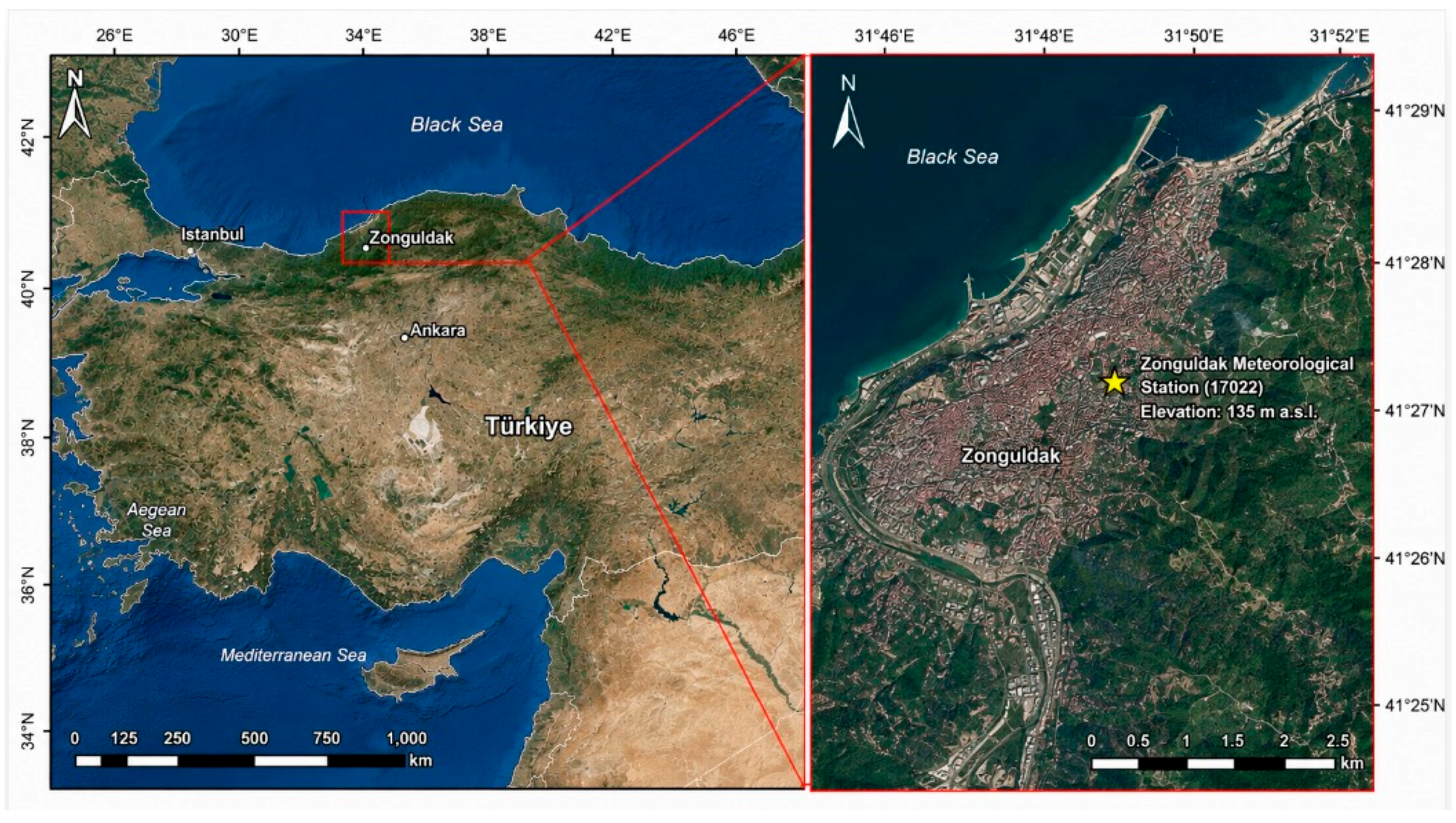
The meteorological observations used in this study were obtained from the Zonguldak Meteorological Station (Station ID: 17022), located at approximately 41.45° N and 31.79° E, at an elevation of 135 m above sea level. The station is located along the western Black Sea coast of Türkiye, and its location is shown in Figure 1. The surrounding area is characterized by a humid coastal environment, complex topography, river valleys, and moderately elevated mountainous terrain [28]. The region is strongly influenced by maritime conditions due to its location along the Black Sea, and the complex topography contributes to local-scale variations in temperature, precipitation, humidity, and wind conditions. These characteristics make Zonguldak a relevant case study for investigating monthly air temperature modelling in a humid coastal environment.

The region receives abundant precipitation and has rich surface water resources, consistent with the climatic characteristics of the Black Sea Region [3,28]. The maritime influence moderates seasonal temperature extremes; summers are generally mild, while winter temperatures are typically less severe than in the more continental parts of Türkiye [3]. Therefore, the study station provides a relevant local setting for investigating how correlated meteorological variables, including thermal, moisture, precipitation, wind, and seasonal components, contribute to monthly mean air temperature variability under humid coastal conditions. This setting is particularly relevant for station-scale environmental and climatological assessment because humid coastal environments are affected by coupled atmosphere–land–sea interactions, hydroclimatic variability, and local-scale environmental conditions that require reliable and interpretable climate information.

2.2. Dataset

The dataset used in this study consists of monthly meteorological observations from a station located in Zonguldak, a humid coastal province in the Western Black Sea Region of Türkiye, covering the period from January 2000 to December 2022. The data were obtained from the General Directorate of Meteorology of the Ministry of Environment, Urbanization and Climate Change of the Republic of Türkiye. The available dataset did not include detailed metadata on instrument changes, station relocation, observation-practice changes, or homogenization procedures; therefore, these aspects were not evaluated in the present study. The same underlying Zonguldak meteorological dataset was previously used by Arslan et al. [27]. However, the present study reanalyzes the original meteorological variables with a different methodological objective, namely to evaluate model stability, model-specific predictor relevance, and the effect of meteorological multicollinearity on monthly air temperature modelling. The full dataset includes 276 monthly observations, corresponding to 23 years of monthly records. Each calendar month is represented by 23 observations. Because the analysis is based on a single station, the observations should not be interpreted as spatially representative of the entire Zonguldak province. The station is used here as a local case study, while broader spatial representativeness would require observations from additional stations.

Monthly mean air temperature, expressed in °C, was taken as the target variable. All predictors and the target refer to the same calendar month. Therefore, the present analysis represents a contemporaneous monthly temperature modelling task rather than future temperature forecasting. Because the target variable is available from the same station record, the models developed here are not intended to replace direct observations of monthly mean air temperature at the study site. Their role in the present study is primarily methodological, namely to examine how model choice, predictor correlation, and predictor ablation affect reconstruction accuracy, stability, and model-specific predictor relevance. The predictors included month, maximum air temperature ($T_{max}$, °C), minimum air temperature ($T_{min}$, °C), mean relative humidity (RH_mean, %), maximum precipitation (P_max, mm), total precipitation (P_total, mm), prevailing mean wind speed (WS_mean, m s⁻¹), maximum wind speed (WS_max, m s⁻¹), prevailing wind direction, and maximum wind direction. Together, these variables represent the main thermal, moisture, precipitation, wind, and seasonal conditions included in the station-scale meteorological dataset.

The meteorological data were supplied by the General Directorate of Meteorology as monthly records, and no aggregation from daily or sub-daily observations was performed by the authors. Detailed information on the observation-level aggregation procedures used to derive the supplied monthly variables was not included in the available dataset documentation. Therefore, the variables were analyzed according to the monthly records provided by the data source.

Since monthly mean temperature is directly related to monthly minimum and maximum temperatures, the full-predictor model was not treated as a completely independent prediction setting. Instead, it was regarded mainly as a thermal reconstruction scenario. Additional models were therefore developed after removing $T_{min}$and $T_{max}$. A seasonality-only scenario was also considered to determine how much of the model performance could be explained by the annual temperature cycle alone. The dataset was also examined for missing observations before preprocessing. Accordingly, the full-predictor scenario was interpreted primarily as a thermal reconstruction setting, whereas the reduced-predictor scenario was used to evaluate broader climatological predictability based on seasonal and non-thermal meteorological information.

Month and wind direction were treated as circular variables. Using their original numerical values would introduce artificial discontinuities; for instance, December and January are consecutive months, although they are represented by 12 and 1. The same applies to wind directions of 0° and 360°, which are numerically distant but physically adjacent. To keep this circular structure, sine and cosine transformations were used [2,21]. Month, prevailing wind direction, and maximum wind direction were represented by Month_sin, Month_cos, PrevailingWind_sin, PrevailingWind_cos, MaximumWind_sin and MaximumWind_cos, respectively. The raw month index was used only to construct Month_sin and Month_cos and was not retained as a separate predictor in the model-training matrix. Similarly, the original angular wind-direction variables were replaced by their sine and cosine components and were not included as additional raw predictors. Records with unavailable or undefined wind-direction information were not assigned arbitrary angular values; instead, the corresponding circular components were handled within the same training-based missing-value preprocessing framework applied to the other predictors. These transformed variables were used in the prediction matrix with the other meteorological variables.

Table 2. Descriptive statistics of the target variable and predictors used in the modelling framework.

Variable	Role	Unit	Mean	SD	Min	Max	Missing
T_mean	Target	°C	14.359	6.068	2.800	25.700	0
$T_{max}$	Predictor	°C	25.772	5.206	13.400	39.500	0
$T_{min}$	Predictor	°C	6.228	6.725	−6.700	19.000	0
RH_mean	Predictor	%	74.778	5.478	60.400	91.800	0
P_max	Predictor	mm	31.512	20.870	0.000	114.400	0
P_total	Predictor	mm	92.688	61.286	0.000	306.600	60
WS_mean	Predictor	m s−1	2.264	0.394	1.200	3.500	0
WS_max	Predictor	m s−1	15.782	3.821	7.700	32.900	14
Month_sin	Predictor	dimensionless	0.000	0.708	−1.000	1.000	0
Month_cos	Predictor	dimensionless	0.000	0.708	−1.000	1.000	0
PrevailingWind_sin	Predictor	dimensionless	0.477	0.497	−1.000	1.000	0
PrevailingWind_cos	Predictor	dimensionless	−0.439	0.578	−1.000	1.000	0
MaximumWind_sin	Predictor	dimensionless	−0.166	0.659	−1.000	1.000	15
MaximumWind_cos	Predictor	dimensionless	0.058	0.734	−1.000	1.000	15

summarizes the descriptive statistics of the target variable and all predictors used in the modelling framework, including their units, mean, standard deviation (SD), minimum (Min), maximum (Max), and number of missing observations. Descriptive statistics were calculated prior to missing-value imputation; for variables containing missing observations, the available values were used in the calculation. Cyclically transformed variables were summarized after the corresponding sine and cosine transformations.

Missing observations were concentrated in a limited subset of variables. Total precipitation (P_total) contained 60 missing monthly observations, maximum wind speed (WS_max) contained 14, and maximum wind direction contained 15 missing records; the remaining target and meteorological variables were complete. The missing maximum-wind-direction records resulted in corresponding missing values in both of its sine and cosine components. The missing P_total observations showed a distinct temporal but not seasonal pattern. All 60 missing records occurred during 2000–2004, with 12 missing monthly observations in each of these five years, whereas no P_total values were missing during 2005–2022. Across calendar months, the missing observations were distributed uniformly, with five missing records for each month from January to December. The temporal and seasonal distributions of missing P_total observations are provided in Supplementary Table S1.

2.3. Multicollinearity Diagnostics

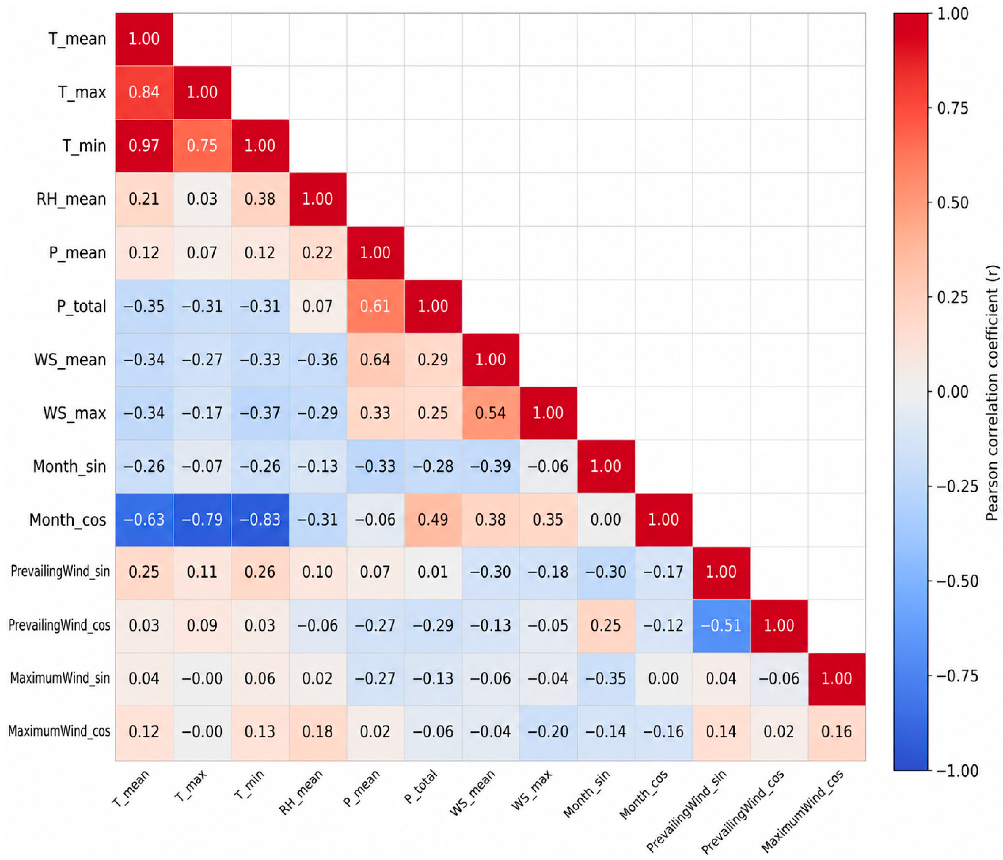
Before model training, the correlation structure of the predictor matrix was examined to characterize predictor correlation and potential multicollinearity. Pairwise Pearson correlation coefficients were calculated among all continuous and transformed predictors to identify associated or potentially redundant meteorological variables. The correlation analysis was performed on the variables after cyclical transformation and before missing-value imputation. For variable pairs containing missing observations, Pearson correlation coefficients were calculated using the available paired observations. In addition, the variance inflation factor (VIF) was computed for each predictor to assess its linear dependence on the remaining predictors. For a predictor ${\mathit{x}}_{\mathit{j}}$, VIF was defined as:

$$\mathit{V}\mathit{I}{\mathit{F}}_{\mathit{j}}={\displaystyle \frac{\mathbf{1}}{\mathbf{1}-{\mathit{R}}_{\mathit{j}}^{\mathbf{2}}}}$$

(1)

where ${\mathit{R}}_{\mathit{j}}^{\mathbf{2}}$ is obtained by regressing ${\mathit{x}}_{\mathit{j}}$ on all remaining predictors. Higher values indicate stronger linear dependence among predictors and a greater risk of coefficient instability [29]. The resulting Pearson correlation matrix was visualized as a heatmap to facilitate evaluation of the predictor correlation structure.

To further evaluate the global conditioning of the predictor matrix, the condition number was calculated from the standardized design matrix. These diagnostics were used to characterize the extent and distribution of predictor dependence in the monthly meteorological dataset and to provide context for comparing regularized and latent-variable regression models with the other modelling approaches. The multicollinearity diagnostics were not used as a feature-selection step; rather, they were used to support the methodological interpretation of model behavior under correlated climatological and Earth system predictors.

2.4. Data Preprocessing

ML algorithms are significantly affected by the quality, scale, and distribution of input data; therefore, an appropriate preprocessing stage is essential for reliable model training and evaluation [5,30]. Several preprocessing steps were applied before model fitting, including missing-value imputation, feature scaling, cyclical-variable transformation, and response-variable transformation.

Missing values were imputed using calendar-month-specific medians to preserve the seasonal structure of the meteorological variables. This strategy was adopted because missing-data treatment in meteorological time series should account for their temporal and seasonal characteristics rather than relying on global summary statistics [31,32]. For each training fold, the median of each numerical predictor was calculated separately for each calendar month, and missing values in the corresponding validation or test fold were replaced using the month-specific median estimated exclusively from the training data. If a month-specific estimate was unavailable within a training fold, the overall median calculated from that training fold was used as a fallback. The imputation procedure was implemented as the first step of the preprocessing pipeline. Month-specific statistics were therefore re-estimated independently within every inner and outer CV training fold before hyperparameter optimization and model fitting. Consequently, all imputation parameters were derived exclusively from the corresponding training data and then applied unchanged to the associated validation or test data, thereby preventing information leakage [33]. Monthly medians were preferred over monthly means because several meteorological predictors, particularly precipitation-related variables, exhibited positively skewed distributions, making the median a more robust estimator while preserving the seasonal structure of the data.

Feature scaling was applied according to the requirements of the regression algorithms. SVR, Ridge, Lasso, ElasticNet, and PLS are affected by differences in predictor scales because their estimation procedures involve distance measures, regularization penalties, or latent components [4,15]. For these models, numerical predictors were standardized using z-score normalization, where each variable was transformed by subtracting the training-fold mean and dividing by the corresponding training-fold standard deviation. Tree-based models are generally insensitive to monotonic rescaling of input variables [4]. Predictor scaling was not applied for RF, GB, and XGBoost.

The response variable was also scaled by using the TransformedTargetRegressor class in the Scikit-learn library. This improved numerical stability during model training and allowed predictions to be converted back to the original temperature unit during the evaluation phase. All error metrics were calculated in degrees Celsius and interpreted directly in the original unit of monthly mean air temperature. The scaling and inverse-transformation procedures were applied independently within each training fold, thereby avoiding information leakage and enabling consistent comparison of the regression models under the same preprocessing framework.

2.5. Predictor Scenarios and Ablation Analysis

This study considered three predictor scenarios to evaluate the dependence of model performance and model-specific predictor relevance on dominant thermal predictors. The first scenario used the full predictor set, including minimum temperature, maximum temperature, relative humidity, precipitation, wind variables, and cyclical seasonal components. This full-predictor scenario was interpreted primarily as a thermal reconstruction reference because minimum and maximum temperature contain direct information related to monthly mean temperature. The second scenario excluded minimum and maximum temperature from the predictor set while retaining relative humidity, precipitation, wind variables, and seasonal components. This reduced-predictor setting was used to assess whether the models could capture monthly mean temperature variability beyond direct thermal predictors. This non-thermal scenario represented the principal setting for assessing broader climatological predictability beyond direct thermal information. The third scenario used only the sine and cosine components of month as a seasonality-only baseline. This baseline was included to quantify how much of the predictive skill could be explained by the annual cycle alone. It therefore served as a seasonal baseline for evaluating the incremental contribution of humidity, precipitation, and wind-related variables. In the seasonality-only setting, OLS using Month_sin and Month_cos corresponds to a first-order harmonic regression [21], representing the annual cycle through continuous sine and cosine terms. This model was kept distinct from the 12-category monthly climatology baseline. For the monthly climatology baseline, the mean target value was calculated separately for each calendar month using only the observations in the corresponding outer-training set. Each observation in the outer-test set was then assigned the training-set mean corresponding to its calendar month. Thus, the 12 monthly climatological means were re-estimated independently within each outer CV fold. The monthly climatology baseline is equivalent to an OLS formulation with calendar-month indicator variables in terms of the fitted monthly means, but it is distinct from the first-order harmonic OLS model based on Month_sin and Month_cos. All predictor scenarios in the ablation analysis were evaluated using the same pre-generated outer-CV splits, matched test observations, and fixed random seeds, with the same preprocessing, tuning, and evaluation workflow applied to each scenario.

Comparisons among these scenarios allowed the contribution of dominant thermal variables to be distinguished from that of seasonal and hydrometeorological information. Therefore, the ablation analysis was used to distinguish direct temperature reconstruction from broader climatological model behavior under meteorological multicollinearity, thereby clarifying whether the models provide predictive information beyond the dominant thermal variables.

Because P_total contained a comparatively large proportion of missing observations (60 of 276; 21.7%), an additional sensitivity analysis was performed to evaluate whether the non-thermal results depended materially on its inclusion and imputation. The non-thermal analysis was repeated after completely excluding P_total from the predictor set, while retaining the same repeated nested CV design, outer-fold partitions, preprocessing procedures, hyperparameter tuning framework, and evaluation metrics used in the primary analysis. Performance obtained without P_total was compared with the corresponding original non-thermal results using fold-averaged MAE, RMSE, and $R^2$.

2.6. ML Models

In addition to the eight primary regression and ML models, reference models and simple baselines were included to provide context for model performance. For direct thermal reconstruction, the arithmetic midpoint of monthly minimum ($T_{mid}$) and maximum temperatures was used as a simple benchmark and was defined as:

$$T_{mid}={\displaystyle \frac{(T_{min}+T_{max})}{2}}$$

(2)

where $T_{min}$ and $T_{max}$ denote the monthly minimum and maximum air temperatures, respectively. OLS and Huber regression were retained as linear and robust reference models, respectively, within the common comparison framework. They were not fitted as separate ${\displaystyle \frac{T_{min}}{T_{\text{max-}only}}}$ baselines. Eight primary regression and ML algorithms were evaluated to compare their predictive performance. The selected models represent different methodological families, including latent-variable regression, regularized linear regression, kernel-based regression, bagging-based ensemble learning, and boosting-based ensemble learning. This model set was chosen to evaluate whether simpler and more interpretable models can provide performance comparable to, or more stable than, more flexible nonlinear models in a correlated monthly meteorological dataset representing station-scale Earth system observations. The eight primary models were PLS, Ridge, Lasso, ElasticNet, SVR, RF, GB, and XGBoost. OLS and Huber regression were additionally included as linear and robust reference models, respectively.

PLS performs simultaneous dimensionality reduction and regression by extracting latent components that explain the covariance structure between the predictor matrix and the response variable. This makes PLS particularly suitable for datasets in which predictors are strongly correlated, as is common in meteorological and climatological applications. Therefore, PLS was included as a latent-variable method for addressing multicollinearity while retaining predictive interpretability through component-based modelling [15].

Ridge regression introduces an L2 regularization penalty into the ordinary least squares method to prevent overfitting and reduce variance in the presence of multicollinearity [8,34]. The regularization strength is controlled by the hyperparameter $\alpha$.

Lasso regression applies an L1 penalty based on the sum of the absolute values of the regression coefficients, allowing some coefficients to shrink to zero and thereby enabling feature selection [9,34]. ElasticNet combines L1 and L2 penalties, thereby integrating the variable-selection capability of Lasso with the coefficient-stabilizing properties of Ridge regression [13,34]. Its behavior is controlled by the overall regularization parameter α and the L1 mixing parameter (l1_ratio). This combination is useful when groups of correlated predictors are present, because it can improve stability while retaining partial feature-selection capability.

SVR addresses nonlinear regression problems by defining an error-tolerance margin and penalizing deviations outside this margin. Nonlinear relationships can be represented through kernel functions that implicitly map the predictors into a higher-dimensional feature space [10]. In this study, SVR was included to evaluate whether a kernel-based nonlinear model provides additional benefit over linear and regularized models for monthly temperature modelling [7,35].

RF is a bagging method that combines multiple decision trees. RF constructs numerous decision trees using randomly selected samples and subsets of variables from the dataset. The final prediction is obtained by averaging the outputs of these trees, thereby improving the model’s generalization performance [11]. GB is a boosting-based ensemble approach that constructs weak learners sequentially, with each new learner aiming to reduce the prediction errors of the preceding ensemble [12]. XGBoost is an optimized version of GB that includes regularization, tree pruning, and computational enhancements to improve predictive performance and training efficiency [14]. These tree-based models were included to test whether flexible nonlinear ensemble methods outperform more constrained linear, regularized, and latent-variable approaches in a monthly climatological dataset characterized by correlated predictors [7,36,37].

2.7. Model Training and Nested CV

Model training and evaluation were performed using nested CV. The inner loop was used for hyperparameter tuning, while the outer loop was used to estimate out-of-sample model performance while reducing bias associated with model selection [19,20,38]. Thus, model optimization and final performance evaluation were conducted at separate stages. In this framework, hyperparameters were selected only using the training portion of each outer split, while the corresponding outer test split was used only for final model evaluation [38].

The nested CV framework included outer and inner loops. In the outer loop, 5-fold CV was implemented using RepeatedKFold with 15 repeats, resulting in 75 outer test evaluations. This helped reduce the impact of random data splitting and provided a more dependable estimate of model performance on unseen data [38,39]. The nested CV procedure was designed to compare out-of-sample predictive performance and model stability across alternative data partitions rather than to simulate an operational time-series forecasting setting.

In the inner loop, hyperparameter optimization was performed using GridSearchCV with 5-fold KFold CV within each outer training set. This separation prevented hyperparameter selection from influencing the corresponding outer-loop performance evaluation. All preprocessing operations, including calendar-month-specific missing-value imputation, predictor scaling, and response-variable transformation, were estimated using only the corresponding training data and then applied to the validation or test data to avoid information leakage [33]. Root Mean Square Error (RMSE) was used as the primary criterion for hyperparameter optimization because it is expressed directly in degrees Celsius, penalizes larger prediction errors more strongly than Mean Absolute Error (MAE), and provides an appropriate optimization objective for continuous temperature prediction [40]. This property is particularly advantageous for meteorological applications, where occasional large prediction errors may have greater practical consequences than small deviations. Furthermore, unlike percentage-based metrics, RMSE does not suffer from instability for observations close to 0 °C, making it more appropriate for air temperature data. The hyperparameter combination yielding the lowest mean RMSE within the inner CV loop was selected for each model. Model performance was subsequently evaluated using MAE, RMSE, and $R^2$ on the corresponding outer test folds, where MAE provides an intuitive measure of average prediction error and R² quantifies the proportion of variability in the observed response accounted for by the fitted model relative to a mean-response baseline.

The hyperparameter search spaces used during inner-loop optimization are provided in

Table 3. Hyperparameter search space used during inner-loop optimization.

Model	Hyperparameter	Search Values
Huber	alpha epsilon	{0.0001, 0.001, 0.01, 0.1} {1.2, 1.35, 1.5}
PLS	n_components	1 to p
Ridge	alpha	{0.01, 0.1, 1, 10, 100}
Lasso	alpha	{0.001, 0.01, 0.1, 1, 10}
ElasticNet	alpha l1_ratio	{0.001, 0.01, 0.1, 1} {0.2, 0.5, 0.8}
SVR	C epsilon gamma	{1, 10, 100} {0.05, 0.1, 0.2} {“scale”, 0.1, 0.01}
RF	n_estimators max_depth min_samples_leaf	{200, 400} {None, 6, 12} {1, 2, 5}
GB	n_estimators learning_rate max_depth	{200, 400} {0.05, 0.1} {2, 3}
XGBoost	n_estimators learning_rate max_depth subsample colsample_bytree min_child_weight reg_alpha reg_lambda	{300, 600} {0.03, 0.05, 0.1} {2, 3, 4} {0.8, 1.0} {0.8, 1.0} {1, 5} {0.0, 0.1} {1.0, 5.0}

Note: Hyperparameter optimization was conducted within the inner loop of the nested CV framework using five-fold KFold CV. The hyperparameter combination yielding the lowest mean RMSE was selected and subsequently evaluated on the corresponding outer test data. Here, $p$ denotes the number of predictors in the corresponding predictor scenario after preprocessing. OLS is not included in Table 3 because it has no tuned hyperparameters.

. The selected ranges were chosen to represent different levels of regularization and model complexity while keeping the repeated nested CV procedure computationally feasible. For tree-based models, the ranges also covered variation in ensemble size, tree depth, learning rate, and sampling-related parameters. After hyperparameter selection, the optimized model was refitted on the full outer training set and evaluated on the corresponding outer test set. This repeated splitting procedure was used to reduce sensitivity to a single random partition and to characterize variability in out-of-sample performance across alternative data splits [38,39].

Because hyperparameter optimization was performed independently within each outer training fold, the selected values were not necessarily identical across the 75 outer evaluations. The selection frequencies of the tuned hyperparameters, including the number of PLS components, are therefore reported separately for the full-predictor, non-thermal, and seasonality-only scenarios in Supplementary Table S2.

Because monthly meteorological observations are temporally ordered and exhibit pronounced seasonal patterns, a supplementary rolling-origin (expanding-window) validation was conducted to assess temporal robustness under a strictly chronological validation setting [21,22]. An initial five-year period was used for model training, after which the subsequent calendar year was used for testing. The training window was then expanded sequentially, yielding 18 annual test periods (2005–2022). Thus, model training for each test year used only observations from preceding years, while contemporaneous predictor values from the held-out test year were used to estimate the corresponding monthly mean temperatures. This analysis complemented the repeated nested CV results by providing an additional assessment of model performance under a strictly chronological validation framework. For the monthly climatology baseline, the 12 calendar-month means were recalculated separately within each expanding training window using only observations from years preceding the corresponding test year, and each month of the held-out year was predicted using the corresponding training-window monthly mean. Additional implementation details for the validation design and the explicit rolling-origin training and test periods are provided in Supplementary Tables S3 and S4.

For the rolling-origin validation, hyperparameters were re-selected independently at each forecast origin using only the observations available in the corresponding expanding training window. Hyperparameter optimization was performed using temporally ordered inner validation rather than random K-fold CV. Within each outer training window, the inner splits preserved chronological order, with all training observations preceding the corresponding validation year. The hyperparameter combination yielding the lowest mean inner-validation RMSE was selected for each model and forecast origin. After hyperparameter selection, the optimized pipeline was refitted using the complete expanding training window and evaluated on the subsequent held-out calendar year. All preprocessing operations, including month-specific missing-value imputation and predictor scaling, were estimated exclusively from the training data within each inner split and were re-estimated from the complete expanding training window before final evaluation. Thus, no observations from the held-out test year were used for preprocessing, hyperparameter selection, or model fitting.

2.8. Performance Metrics and Statistical Analysis

In this study, three complementary performance metrics were employed to evaluate predictive performance: MAE, RMSE, and the coefficient of determination ($R^2$). MAE quantifies the average magnitude of prediction errors in the original unit of the response variable (°C), providing an intuitive measure of typical prediction error. RMSE also measures prediction error in degrees Celsius but assigns greater weight to larger deviations, making it particularly suitable for evaluating regression models in which occasional large errors are of practical importance [40]. Because RMSE penalizes large prediction errors more strongly than MAE and remains stable for observations close to 0°C, it was used as the primary criterion for hyperparameter optimization. R² quantifies the proportion of variability in the observed response accounted for by the fitted model relative to a mean-response baseline. In this study, $R^2$was interpreted strictly as a measure of predictive performance rather than evidence of causal explanation [41]. MAE and RMSE are expressed in degrees Celsius (°C), whereas $R^2$ is dimensionless. The mathematical definitions of these metrics are as follows:

$$MAE={\displaystyle \frac{1}{n}}{\displaystyle {\sum }_{i=1}^n}\left|y_i-{\widehat{y}}_i\right|$$

(3)

$$RMSE=\sqrt{{\displaystyle \frac{1}{n}}{\displaystyle {\sum }_{i=1}^n}{(y_i-{\widehat{y}}_i)}^2}$$

(4)

$$R^2=1-{\displaystyle \frac{{\displaystyle {\sum }_{i=1}^n}{(y_i-{\widehat{y}}_i)}^2}{{\displaystyle {\sum }_{i=1}^n}{({\widehat{y}}_i-\overline{y})}^2}}$$

(5)

where $y_i$ denotes the observed value, ${\widehat{y}}_i$ denotes the corresponding model prediction, $\overline{y}$ denotes the mean of the observed values, and $n$ is the total number of observations [27,40].

To summarize variability in model performance across the repeated outer evaluations, 95% descriptive bootstrap variability intervals were calculated for MAE, RMSE, and $R^2$ using 10,000 bootstrap resamples of the outer-loop metric values. In each bootstrap resample, the mean metric value was recalculated, and the interval bounds were defined by the 2.5th and 97.5th percentiles of the resulting bootstrap distribution (percentile method) [42]. Because the repeated CV evaluations are not statistically independent, these intervals were interpreted descriptively as summaries of variability across alternative data partitions rather than as inferential confidence intervals based on independent observations. Statistical comparisons between models were therefore based on paired MAE values from the 18 annual test periods of the rolling-origin validation. Pairwise differences were assessed using the Wilcoxon signed-rank test [43], and the Holm-Bonferroni correction was applied for multiple comparisons [44]. Pairwise differences in MAE (ΔMAE) were also reported to describe the practical magnitude of the observed performance differences. A negative ΔMAE indicates that the model listed in the corresponding row achieved a lower mean absolute prediction error than the comparison model.

To evaluate the incremental predictive contribution of the non-thermal meteorological predictors beyond the seasonal baseline, paired year-level differences in MAE were calculated using the 18 annual test periods (2005–2022) of the rolling-origin validation. For each model and test year, ΔMAE was defined as MAE_non-thermal − MAE_climatology, such that negative values indicated lower prediction error for the non-thermal model. The mean and median annual ΔMAE values were summarized across the 18 paired test years. To characterize the variability of the mean paired annual difference, 95% percentile bootstrap intervals were calculated using 10,000 bootstrap resamples of the 18 annual ΔMAE values. Paired differences were additionally evaluated using the Wilcoxon signed-rank test, with Holm correction applied across the model-wise comparisons. The number of test years in which each non-thermal model achieved a lower MAE than the monthly climatology baseline was also reported to characterize the temporal consistency of the observed improvement.

2.9. Model-Specific Predictor Relevance Framework

In addition to predictive performance, model-specific predictor relevance was examined to characterize how the fitted models used the available meteorological predictors under correlated-input conditions [45,46,47]. Two complementary approaches were employed: VIP for the PLS model and permutation feature importance for the GB model [15,45,47]. GB was selected for permutation-importance analysis to provide a nonlinear tree-based counterpart to the latent-variable PLS interpretation and to examine whether predictor-relevance patterns differed across substantially different model structures. Its selection was therefore intended to provide a complementary model-specific interpretation rather than to identify the overall best-performing model. These measures were interpreted as indicators of predictive relevance within the fitted model and observed predictor dependence structure, rather than as evidence of independent physical control or causal influence.

For the PLS model, VIP scores were calculated for each outer-fold model obtained during the repeated nested CV procedure. Mean VIP values and the corresponding fold-wise variability intervals were then summarized across the 75 outer validation folds to assess the stability of predictor relevance. Variables with VIP values greater than 1 were interpreted as having above-average model-specific predictive relevance within the fitted PLS representation [15,45]. Thus, the VIP analysis identified the predictors that consistently contributed to the latent PLS representation across the outer validation folds.

For the GB model, permutation feature importance was calculated on each outer-fold test set using 30 repeated permutations per predictor. Mean decreases in test-set R² and the corresponding fold-wise variability intervals were then summarized across the 75 outer validation folds. In this approach, the values of each predictor were randomly permuted while all other predictors were kept unchanged, and the resulting decrease in R² was used as an importance measure [47]. Variables causing larger decreases in test-set R² after permutation were interpreted as having greater model-specific predictive relevance. However, because permutation importance can be affected by correlation among predictors, the results were interpreted as model-specific predictive importance rather than as evidence of independent causal effects [46,47]. Accordingly, these analyses were used to characterize model-specific predictive relevance under the observed correlation structure, while the statistical comparison of predictive performance was based on the full nested CV procedure. Because minimum and maximum temperature are closely related to monthly mean air temperature, their importance was interpreted as evidence of thermal reconstruction capacity rather than as independent causal control of the target variable. This distinction helps avoid overinterpretation of predictor-importance measures under correlated-input conditions.

To complement the individual-predictor analysis under correlated-input conditions, grouped permutation importance was also evaluated for the GB model. Predictors were grouped according to their meteorological roles as thermal, seasonal, precipitation, humidity, and wind variables. The predictors within each group were jointly permuted using the same row permutation within each outer-test fold. Group importance was calculated as the decrease in test-set $R^2$ relative to the corresponding unpermuted model and was summarized across the 75 outer validation folds. The grouped analysis was carried out for both the full-predictor and non-thermal scenarios.

All analyses were conducted in Python 3.9.18 using NumPy 1.26.0, pandas 2.1.4, SciPy 1.11.4, statsmodels 0.14.0, scikit-learn 1.4.2, and XGBoost 1.7.6. A fixed random seed of 42 was used for repeated CV, stochastic model components, and bootstrap resampling where applicable. For Lasso and ElasticNet, the default scikit-learn convergence settings were retained, with a maximum of 1,000 iterations (max_iter = 1000) and a convergence tolerance of 1 × 10⁻⁴ (tol = 1 × 10⁻⁴); coordinate updates used the default cyclic selection scheme.

3. Results

In this study, the monthly mean air temperature in Zonguldak, Western Black Sea Region of Türkiye was modelled and evaluated using long-term meteorological observations of a humid coastal climate. The predictor set included thermal variables, relative humidity, precipitation, wind-related variables, and cyclical terms representing seasonality. These predictors were considered jointly to distinguish direct thermal information from broader seasonal and hydrometeorological contributions.

All regression models were assessed using an identical nested CV procedure. Performance variability was quantified using bootstrap resampling, and pairwise differences between models were evaluated statistically. Predictor-ablation scenarios were subsequently used to determine how strongly model performance depended on thermal, seasonal, and other hydrometeorological information.

3.1. Multicollinearity Patterns in the Predictor Set

Before the models were compared, correlations among the monthly meteorological variables were assessed to identify strongly related predictors. The diagnostic analysis showed that several predictors were strongly correlated, particularly the thermal variables and seasonal components. This indicates that predictor dependence was structured rather than uniformly distributed across the dataset.

Figure 2 presents the Pearson correlation structure of the target variable and predictors. Strong correlations were observed primarily among the thermal and seasonal variables. $T_{min}$and $T_{max}$were positively correlated (r = 0.75), while both thermal predictors showed strong negative correlations with Month_cos (r = −0.92 for $T_{min}$ and r = −0.79 for $T_{max}$). Moderate-to-strong correlations were also observed between P_max and P_total (r = 0.61) and between WS_mean and WS_max (r = 0.54). In contrast, most remaining predictor pairs exhibited weak to moderate linear associations. Thus, predictor redundancy was concentrated mainly within the thermal, seasonal, precipitation, and wind-related variable groups rather than across the full predictor set.

The variance inflation factor analysis supported this localized pattern of collinearity. Minimum temperature exhibited the highest VIF value (VIF = 11.41), while the cyclical seasonal descriptors Month_cos (VIF = 7.61) and Month_sin (VIF = 7.30) also showed relatively high VIF values. In contrast, the remaining meteorological predictors exhibited low VIF values (all <3.4), indicating limited linear dependence among the non-thermal variables. The condition number of the standardized predictor matrix was 9.04, suggesting that the overall predictor matrix was not severely ill-conditioned. Collectively, the correlation, VIF, and condition-number analyses indicate that multicollinearity was primarily confined to the thermal and seasonal predictors rather than affecting the predictor set as a whole. It is also important to distinguish predictor multicollinearity from target-related redundancy. The strong relationship of $T_{min}$and $T_{max}$ with monthly mean temperature primarily reflects direct thermal information about the response, whereas multicollinearity refers to dependence among the predictors themselves. The VIF and condition-number results indicate that the latter was localized rather than severe across the full predictor matrix.

3.2. Reference Performance Under the Full-Predictor Reconstruction Scenario

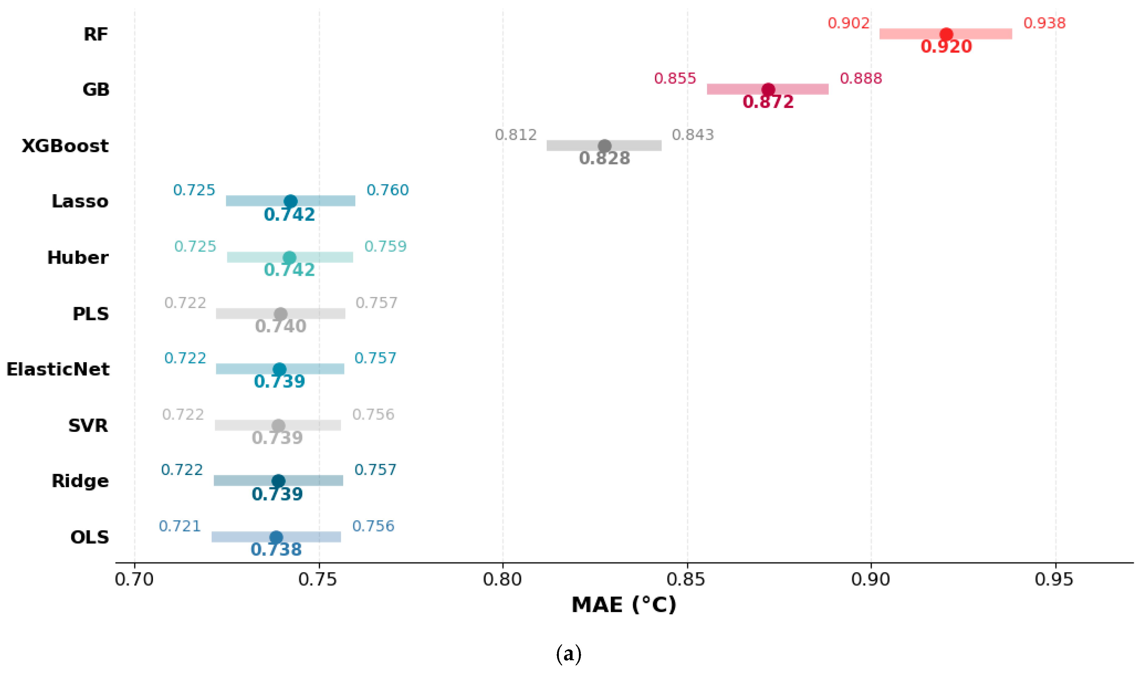
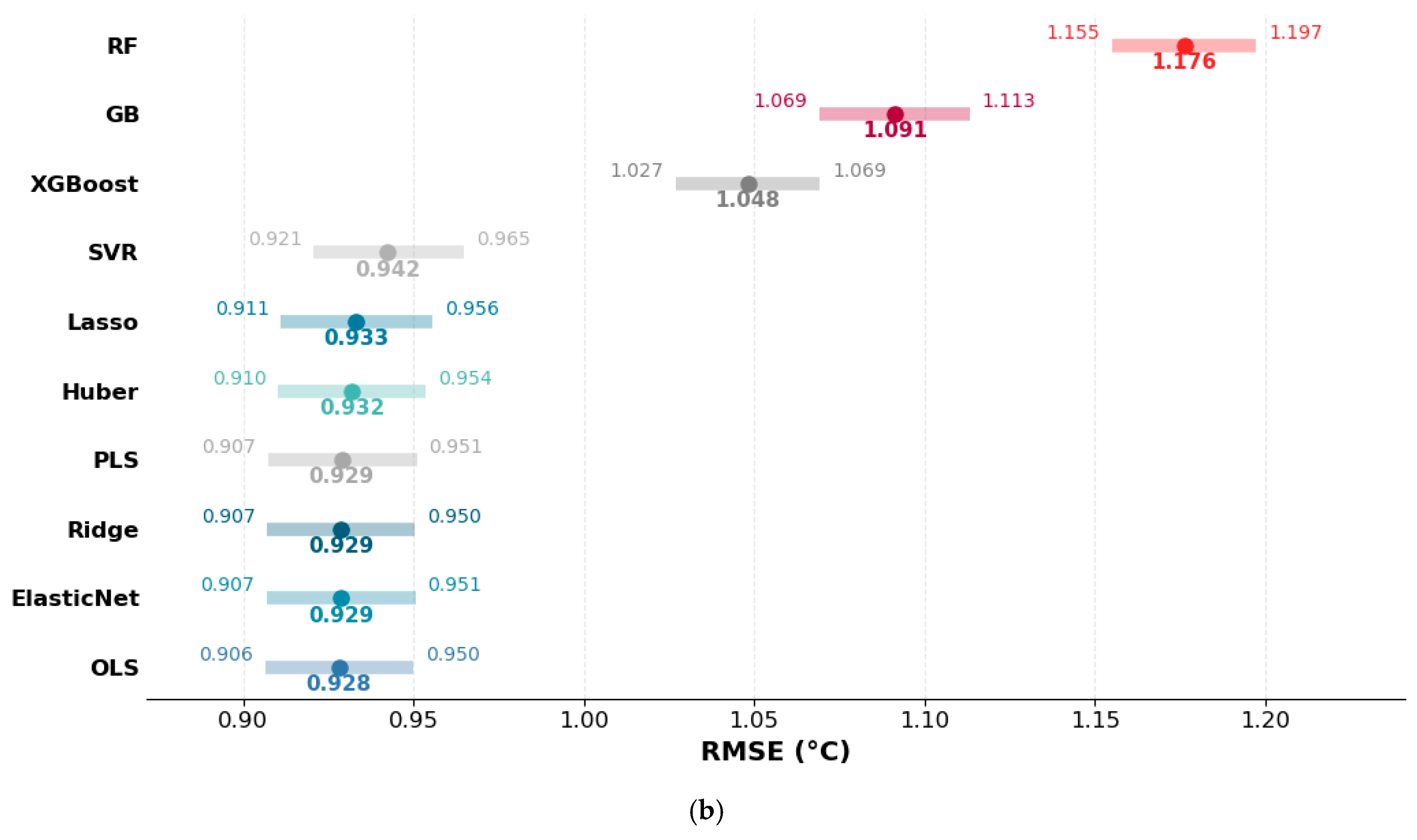
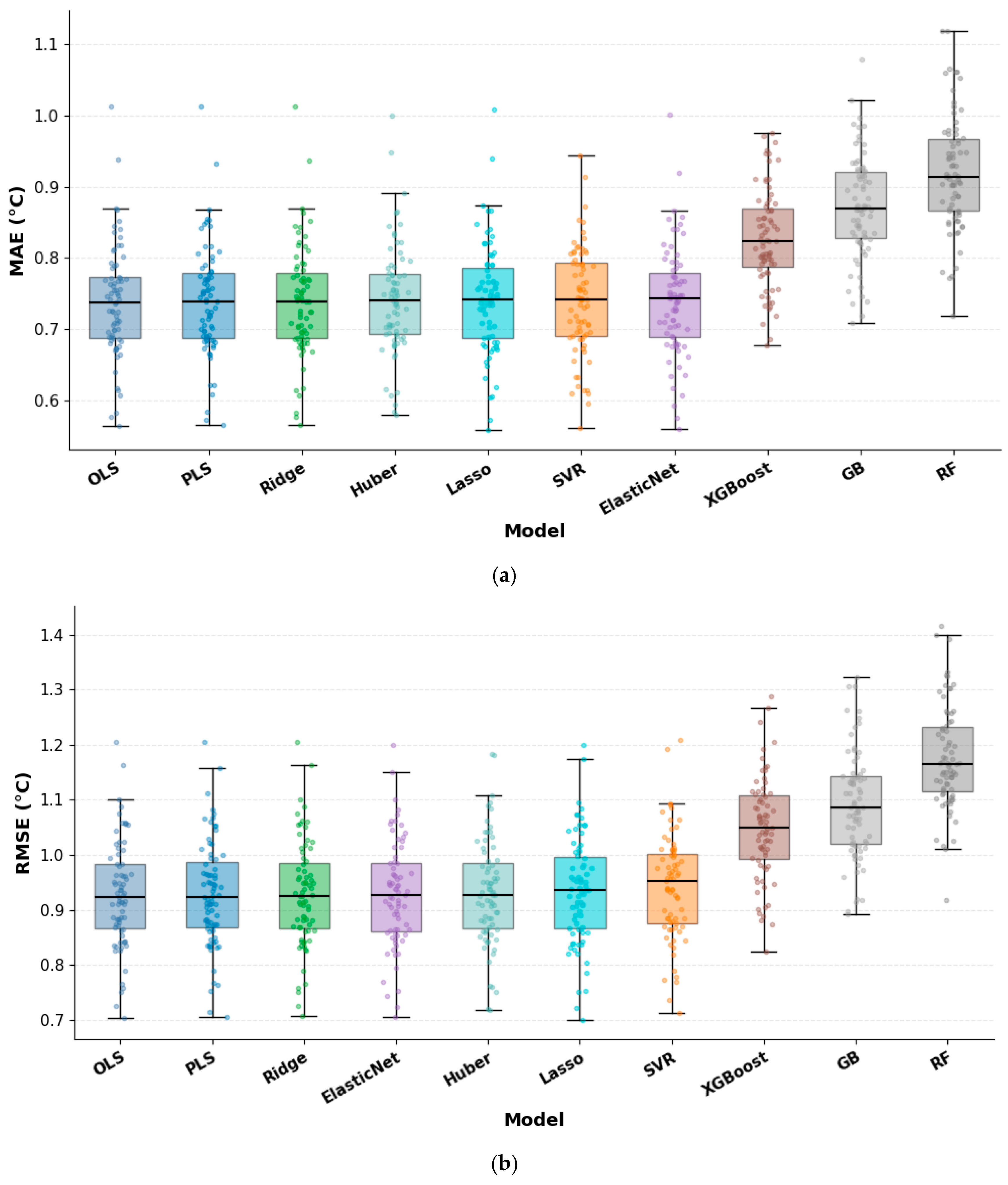
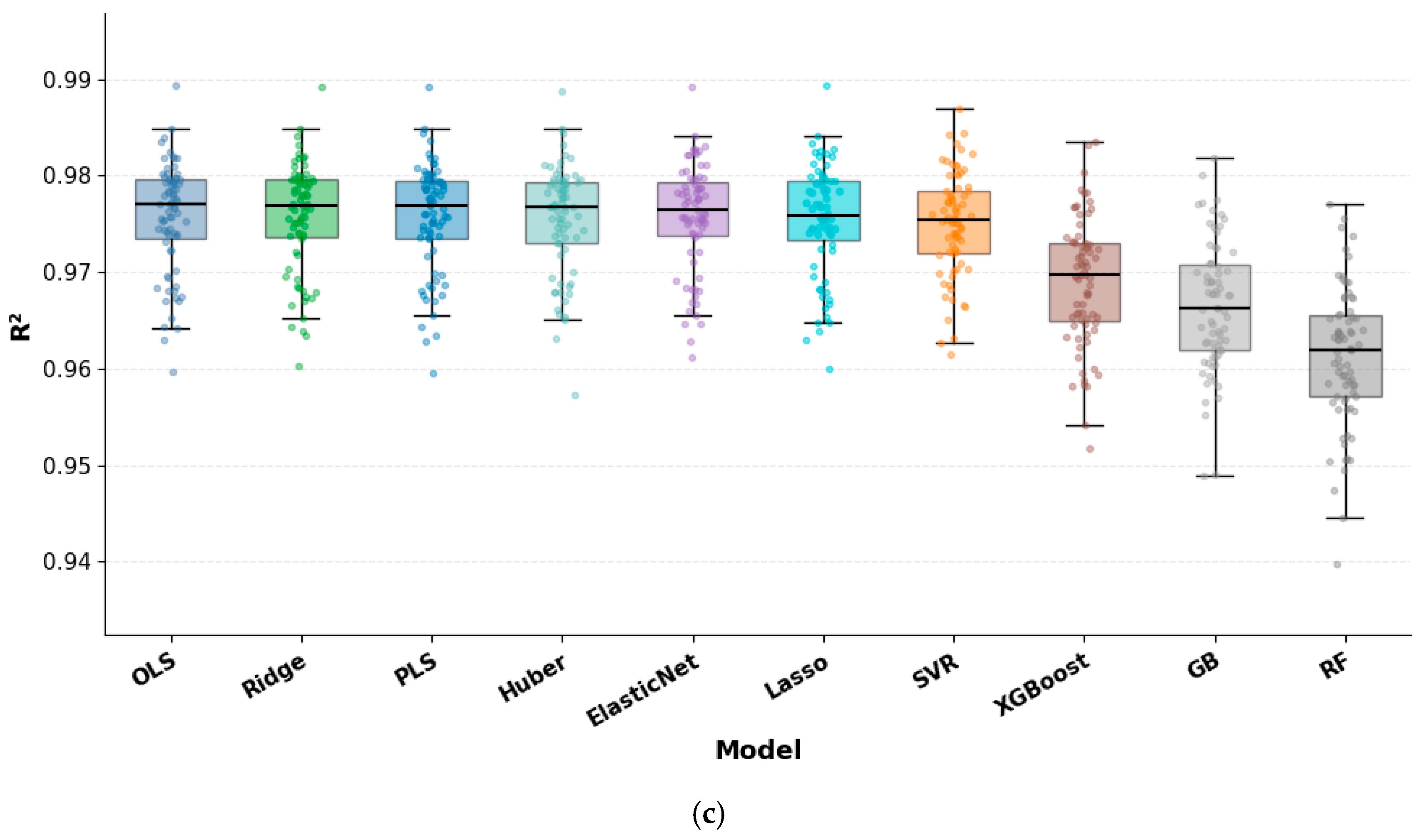
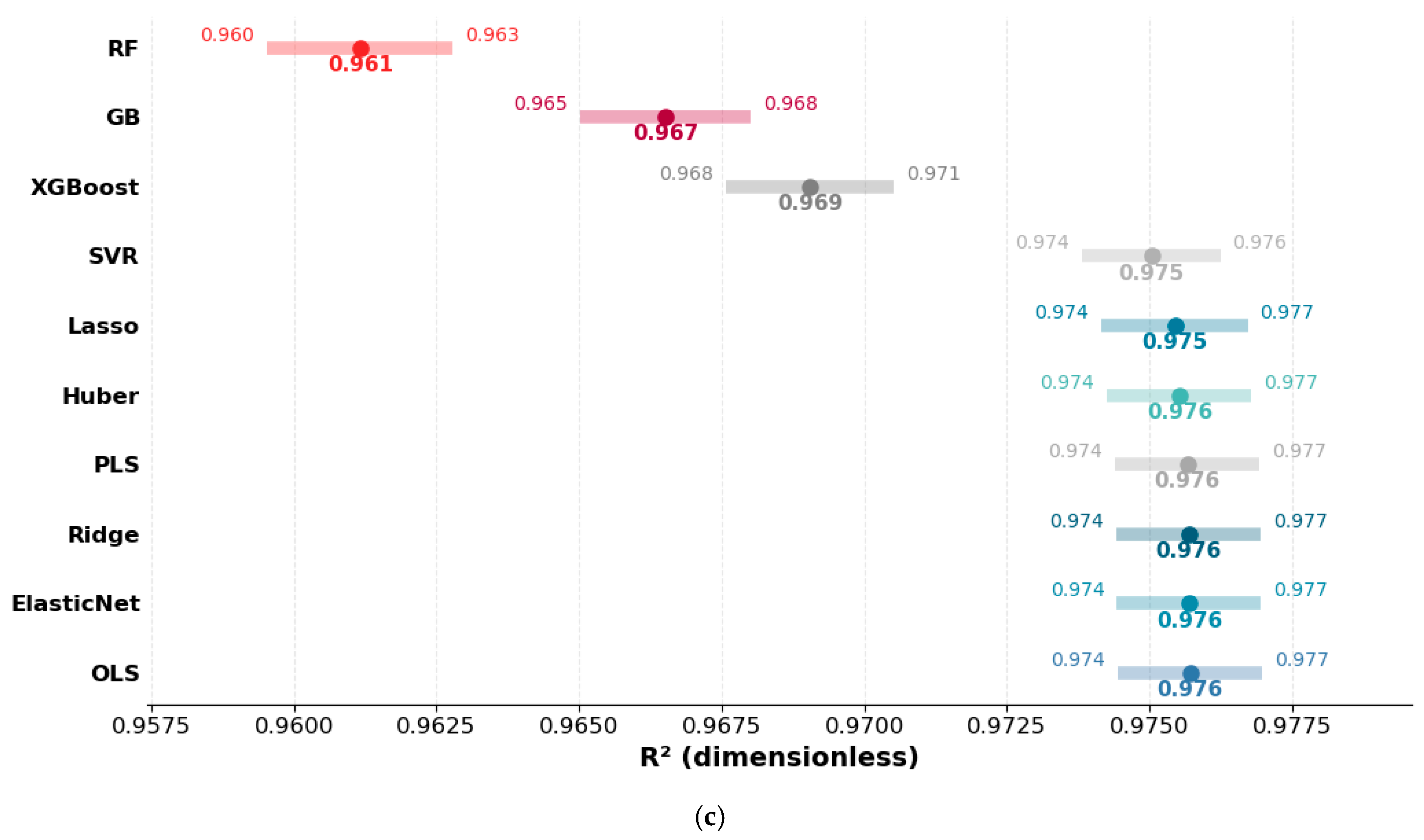
The full-predictor scenario was evaluated primarily as a reference thermal-reconstruction setting because $T_{min}$and $T_{max}$contain direct information closely related to monthly mean temperature. Model performance under this reference scenario is summarized in Figure 3. Ordinary least squares (OLS) achieved a mean MAE of 0.738 °C and an RMSE of 0.928 °C. Ridge, ElasticNet, PLS, Huber, Lasso, and SVR produced similar results, with MAE values of approximately 0.74 °C and mean $R^2$ values of approximately 0.975–0.976. The close agreement among these models, together with the overlap in their descriptive bootstrap variability intervals, indicates that the full-predictor scenario did not identify a single clearly superior linear, regularized, latent-variable, or kernel-based model.

The tree-based ensemble models produced higher errors. XGBoost showed the lowest error among these methods, with an MAE of 0.828 °C and an RMSE of 1.048 °C, followed by GB with an MAE of 0.872 °C and an RMSE of 1.091 °C. RF yielded the largest errors, with an MAE of 0.920 °C and an RMSE of 1.176 °C. Their corresponding mean $R^2$ values were approximately 0.969, 0.967, and 0.961, respectively.

Overall, greater model flexibility did not provide a clear advantage under the full-predictor setting. Because $T_{min}$and $T_{max}$ contain direct information about monthly mean temperature, this scenario is interpreted primarily as a thermal-reconstruction benchmark rather than as evidence of independent prediction from broader meteorological conditions.

3.3. Performance Stability Under the Reference Reconstruction Scenario

Although the mean performance values provide an overall comparison of predictive accuracy, they do not fully describe model stability across different train-test partitions. Therefore, the distributions of the outer-loop performance values obtained from the repeated nested CV procedure were examined (Figure 4). The boxplots indicate that OLS, Ridge, ElasticNet, PLS, Lasso, and Huber exhibited relatively compact performance distributions, reflecting stable predictive behaviour across the 75 outer-test evaluations. SVR also showed relatively consistent performance, although with slightly higher prediction errors than the linear and latent-variable models.

Among the nonlinear models, XGBoost showed lower prediction errors and a more compact distribution than GB and RF, whereas RF exhibited the largest variability, particularly for RMSE and $R^2$. Nevertheless, the overall differences in fold-to-fold variability among the evaluated models were smaller than the corresponding differences in their average prediction errors. These findings indicate that, within the full-predictor reconstruction setting, the primary distinction between the competing models lies in predictive accuracy rather than in the stability of their performance across repeated train-test partitions.

3.4. Pairwise Statistical Comparison Under the Reference Reconstruction Scenario

Pairwise statistical comparisons were based on MAE values obtained for the 18 annual test periods of the rolling-origin validation. This year-level comparison was used to avoid treating the repeated outer-CV evaluations as statistically independent observations. Pairwise differences were assessed using the Wilcoxon signed-rank test, and Holm correction was applied for multiple comparisons. Under the full-predictor scenario, OLS was used as the reference model because it achieved the lowest mean MAE in the rolling-origin analysis. Because differences in average error were generally small for several models, both the magnitude of the MAE difference and the adjusted p-value were considered.

Table 4. Pairwise MAE differences relative to OLS for the full-predictor reconstruction benchmark based on the 18 rolling-origin test years. Positive ΔMAE indicates higher error than OLS.

Comparison Model	ΔMAE (Model − OLS, °C)	Holm-Adjusted p-Value
Ridge	0.003	1.000
ElasticNet	0.007	1.000
PLS	0.007	1.000
Huber	0.007	1.000
Lasso	0.010	1.000
SVR	0.067	0.469
XGBoost	0.127	1.000
GB	0.175	0.077
RF	0.234	0.017
Monthly climatology	0.577	<0.001
Tmin–Tmax midpoint	1.038	<0.001

shows that the differences between OLS and Ridge, ElasticNet, PLS, Huber, and Lasso were very small (ΔMAE ≤ 0.010 °C) and none remained statistically significant after Holm correction. Although SVR, XGBoost, and GB exhibited larger mean MAE differences, these differences were also not statistically significant after adjustment for multiple comparisons. In contrast, RF showed significantly higher prediction error than OLS (ΔMAE = 0.234 °C, adjusted p = 0.017). The two reference baselines, monthly climatology and the $T_{min}-T_{max}$ midpoint, produced substantially larger errors than OLS and both differences remained highly significant (adjusted p < 0.001). Overall, the statistical comparisons indicate that OLS, Ridge, ElasticNet, Lasso, PLS, and Huber were statistically indistinguishable within the full-predictor reconstruction benchmark.

3.5. Predictive Performance Beyond Direct Thermal Information

The ablation analysis was therefore used to distinguish the contribution of direct thermal information from that of seasonal, moisture, precipitation, and wind-related predictors. The same outer-CV partitions were used for all predictor scenarios, allowing the changes in prediction error to be evaluated on matched test observations. The corresponding MAE-based ablation results are summarized in

Table 5. MAE-based ablation results under the three predictor scenarios. ΔMAE values represent paired changes obtained using identical outer test partitions.

Model	Full MAE (°C)	Non-Thermal MAE (°C)	Seasonality-Only MAE (°C)	Δ Full → Non-Thermal (°C)	Δ Non-Thermal → Seasonality (°C)
OLS	0.738	1.173	1.334	0.435	0.161
Huber	0.742	1.177	1.335	0.435	0.158
PLS	0.740	1.178	1.334	0.439	0.156
Ridge	0.739	1.173	1.335	0.434	0.162
Lasso	0.742	1.176	1.336	0.434	0.160
ElasticNet	0.739	1.175	1.336	0.436	0.161
SVR	0.739	1.126	1.270	0.387	0.144
GB	0.872	1.127	1.279	0.255	0.153
RF	0.920	1.222	1.280	0.302	0.057
XGBoost	0.828	1.165	1.282	0.337	0.118

Note: The training-fold monthly climatology baseline yielded an MAE of 1.280 °C, RMSE of 1.649 °C, and $R^2$of 0.923. Positive ΔMAE values indicate an increase in error after predictor removal.

.

As shown in Table 5, removing $T_{min}$and $T_{max}$ increased MAE for all evaluated models. Under the full-predictor scenario, MAE values for the main regression and machine-learning models ranged from approximately 0.74 to 0.92 °C. After the direct thermal predictors were removed, MAE increased to approximately 1.13–1.22 °C. The corresponding $R^2$ values decreased from approximately 0.96–0.98 to approximately 0.93–0.94. The paired increase in MAE after removing $T_{min}$and $T_{max}$ ranged from approximately 0.25 °C for GB to approximately 0.44 °C for PLS. The systematic deterioration across all models indicates that much of the predictive skill in the full-predictor setting depended on the direct thermal information provided by $T_{min}$and $T_{max}$ rather than on broader hydrometeorological information.

In the seasonality-only scenario, MAE values were approximately 1.27–1.34 °C, while the training-fold monthly climatology baseline produced an MAE of approximately 1.28 °C. Adding the non-thermal meteorological predictors reduced MAE relative to the seasonal baseline, but the magnitude of this improvement was model dependent. For example, SVR and GB achieved non-thermal MAE values of approximately 1.13 °C, compared with approximately 1.27–1.28 °C under the seasonal-only setting. Thus, non-thermal meteorological information provided an additional but comparatively modest improvement beyond the annual seasonal cycle, whereas the much larger deterioration from the full to the non-thermal scenario reflected the dominant contribution of direct thermal information.

Taken together, the ablation results reveal a consistent hierarchy in the information provided by the predictor groups. Direct thermal variables accounted for the largest incremental improvement in predictive accuracy, while the annual seasonal cycle explained a substantial proportion of the remaining monthly temperature variability. The additional contribution of the non-thermal meteorological predictors was smaller and varied across models. Model rankings also changed across predictor scenarios, indicating that relative model performance depended on the information available to the algorithms rather than reflecting a uniform advantage of a particular model family. Because P_total contained the largest proportion of missing observations, the robustness of the non-thermal results to this variable was examined in an additional sensitivity analysis. Excluding P_total produced only minor changes in mean MAE for most models. The absolute MAE change was below 0.01 °C for PLS, Ridge, Lasso, ElasticNet, OLS, Huber, RF, and GB. Larger model-specific changes were observed for SVR, for which MAE increased from 1.126 to 1.201 °C (+0.075 °C), and XGBoost, for which MAE decreased from 1.164 to 1.110 °C (−0.054 °C). Thus, removal of P_total did not produce a systematic deterioration in predictive performance across the evaluated model set, indicating that the principal non-thermal findings were not generally dependent on the inclusion and imputation of P_total. Detailed results are provided in Supplementary Table S5.

3.6. Rolling-Origin Temporal Validation

A rolling-origin validation experiment was conducted to examine model performance under a strictly chronological temporal splitting scheme. An initial five-year training period was used, after which each subsequent calendar year was evaluated using models trained only on preceding years, while contemporaneous predictor values from the held-out year were used to estimate monthly mean temperature. The training set was expanded sequentially, resulting in 18 annual test periods from 2005 to 2022. The results are summarized in

Table 6. Rolling-origin validation results for the full and non-thermal predictor scenarios across 18 annual test periods (2005–2022).

Model	Full MAE (°C)	Full RMSE (°C)	Non-Thermal MAE (°C)	Non-Thermal RMSE (°C)
OLS	0.731	0.898	1.187	1.465
Huber	0.738	0.907	1.194	1.464
PLS	0.738	0.907	1.188	1.464
Ridge	0.734	0.901	1.176	1.457
Lasso	0.741	0.905	1.167	1.448
ElasticNet	0.738	0.901	1.167	1.445
SVR	0.798	0.944	1.194	1.459
GB	0.906	1.101	1.157	1.446
RF	0.965	1.196	1.268	1.573
XGBoost	0.859	1.055	1.231	1.534
Monthly climatology	1.309	1.625	1.309	1.625
$T_{min}-T_{max}$midpoint	1.769	2.107	—	—

.

Under the full-predictor scenario, OLS, Ridge, ElasticNet, PLS, Lasso, and Huber again showed similar performance, with mean MAE values of approximately 0.73–0.74 °C. OLS produced the lowest mean MAE (0.731 °C), although the differences within this group were small. SVR showed a somewhat higher MAE (0.798 °C), while XGBoost, GB, and RF produced mean MAE values of 0.859, 0.906, and 0.965 °C, respectively.

The relative ranking changed when $T_{min}$and $T_{max}$ were excluded. Under the non-thermal scenario, GB produced the lowest mean MAE (1.157 °C), followed closely by ElasticNet and Lasso (approximately 1.167 °C) and Ridge (1.176 °C). OLS and PLS yielded MAE values of approximately 1.19 °C. The monthly climatology baseline produced an MAE of 1.309 °C. These results indicate that relative model performance depended on the predictor scenario and that the temporal validation results do not support a general superiority of a single model family across all settings.

Table 6 confirms that the main conclusions remained consistent under the rolling-origin validation framework. After the thermal predictors were excluded, GB, ElasticNet, and Lasso achieved the lowest MAE values under the non-thermal scenario, whereas RF and XGBoost showed comparatively higher errors. The model ranking therefore differed from that observed when direct thermal information was available, indicating that relative model performance depended on the predictor information provided to the algorithms. The full-predictor results are interpreted primarily as a reconstruction reference, whereas the non-thermal results provide a more informative assessment of temporal robustness beyond direct thermal information. Overall, the rolling-origin analysis supports the main patterns observed in the repeated nested CV results under a strictly chronological evaluation framework.

To further examine whether the incremental contribution of the non-thermal predictors beyond the seasonal baseline was consistent across test years, paired annual ΔMAE values were calculated for the 18 rolling-origin test periods. Here, ΔMAE was defined as the MAE of the non-thermal model minus the MAE of the monthly climatology baseline, such that negative values indicate lower prediction error for the non-thermal model. Mean ΔMAE values were negative for all evaluated models and ranged from −0.151 °C for GB to −0.041 °C for RF, indicating relatively small average reductions in prediction error. GB achieved lower MAE than the monthly climatology baseline in 15 of the 18 test years and showed a mean ΔMAE of −0.151 °C, with a 95% percentile bootstrap interval of −0.238 to −0.061 °C. Several other models also achieved lower MAE than the climatology baseline in most test years; however, after Holm correction for multiple model-wise comparisons, only the GB comparison remained statistically significant (adjusted p = 0.047). These results indicate that the additional non-thermal meteorological predictors provided a small and model-dependent improvement beyond the seasonal baseline, rather than a uniformly strong improvement across all model families. Detailed paired year-level results for all models are provided in Supplementary Table S6.

3.7. Model-Specific Predictor Relevance Under Correlated Meteorological Variables

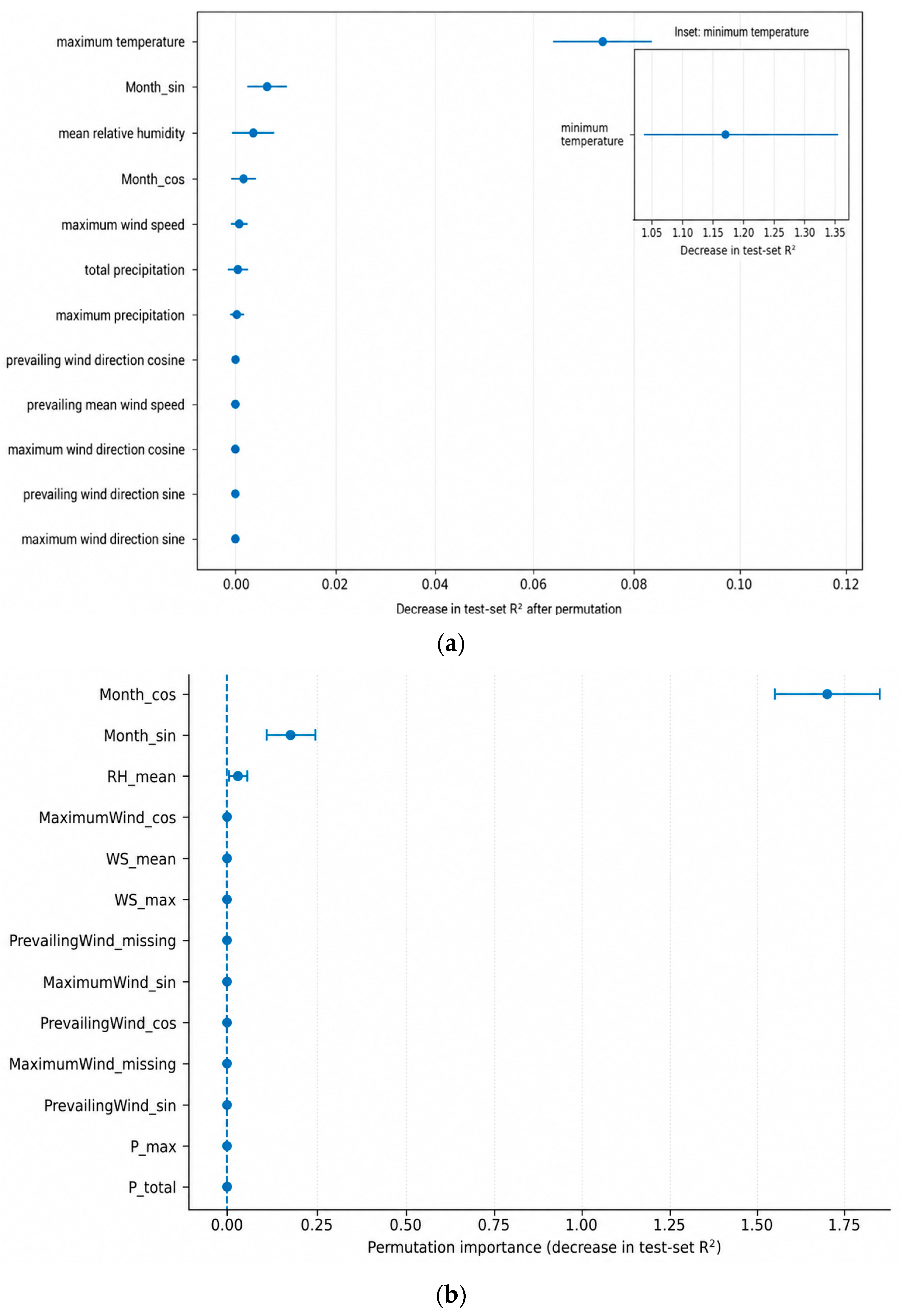
Model-specific predictor relevance was evaluated across the outer validation folds rather than using a single representative fitted model. VIP scores were calculated for the PLS model in each of the 75 outer folds, while permutation importance for GB was calculated on each outer test set using 30 repeated permutations per predictor. The resulting distributions and fold-wise variability intervals are summarized in Figure 5 and Figure 6.

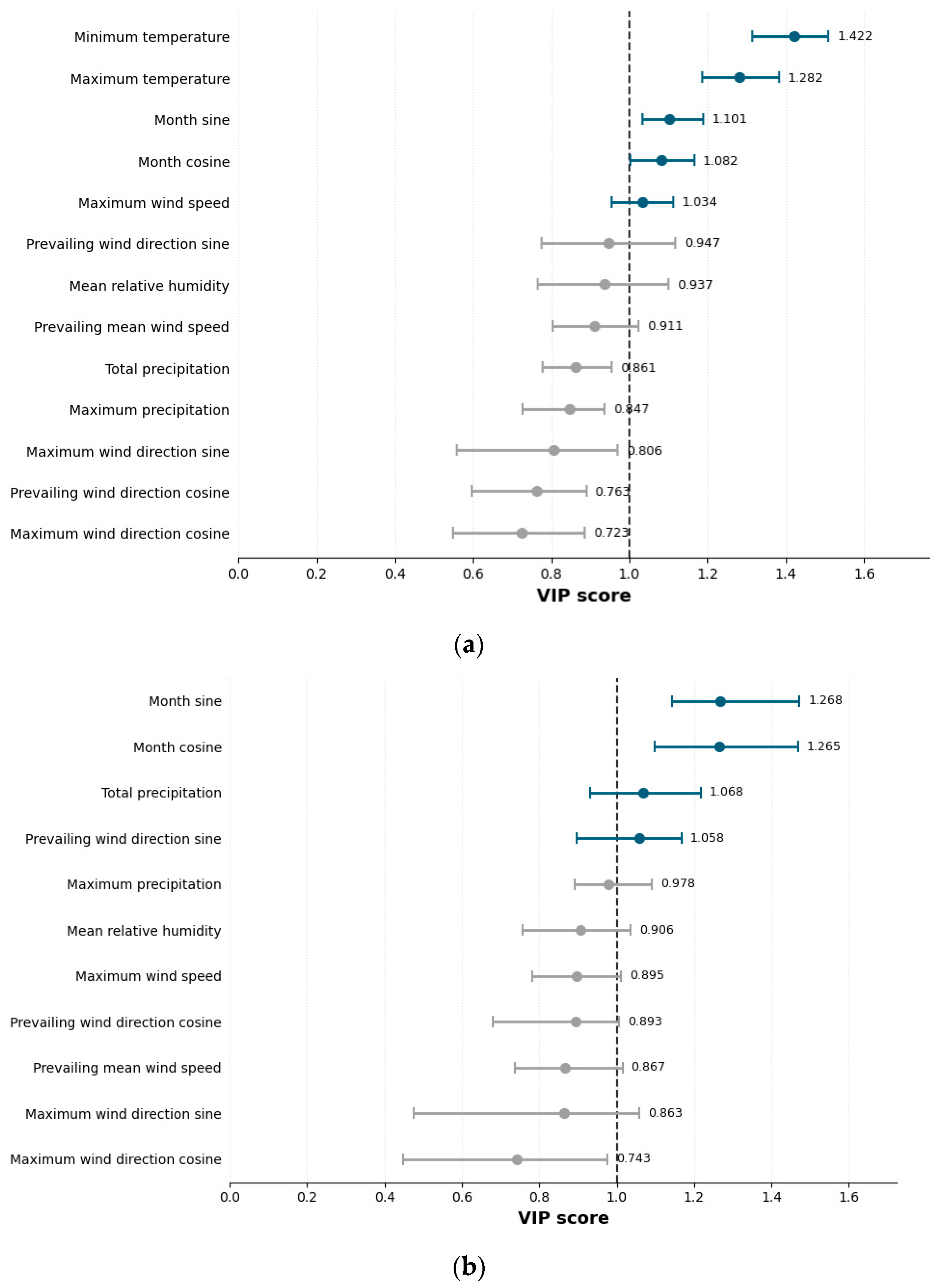
As shown in Figure 5, the VIP analysis revealed distinct patterns of predictor importance under the two predictor scenarios. In the full-predictor scenario (Figure 5a), minimum temperature, maximum temperature, Month_sin, and Month_cos all exhibited mean VIP values above 1, indicating that thermal variables and the annual seasonal cycle contributed most strongly to the fitted PLS model. In contrast, precipitation, relative humidity, and wind-related variables generally showed lower VIP values. After the thermal predictors were removed (Figure 5b), Month_sin and Month_cos became the dominant predictors, with mean VIP values of approximately 1.27, whereas the remaining meteorological variables generally remained closer to or below the VIP = 1 reference level. This shift is consistent with the ablation results and indicates that the annual seasonal cycle becomes the primary source of predictive information in the absence of direct thermal predictors.

As shown in Figure 6, the permutation-importance profile differed substantially across predictor scenarios and from the PLS VIP profile. Under the full-predictor scenario (Figure 6a), minimum temperature produced by far the largest mean decrease in test-set $R^2$ after permutation (1.171), followed by maximum temperature (0.093). The importance estimates for the seasonal components were considerably smaller, while most precipitation, humidity, wind-speed, and wind-direction predictors showed values close to zero. Several wind-direction components exhibited slightly negative mean importance values. Under the non-thermal scenario (Figure 6b), removal of $T_{min}$ and $T_{max}$ produced a pronounced shift toward the seasonal components. Month_cos showed by far the largest mean permutation importance (1.676), followed by Month_sin (0.180), while RH_mean showed a substantially smaller positive importance (0.032). The remaining precipitation and wind-related predictors had mean importance values close to zero. This pattern indicates that the GB model relied predominantly on the annual seasonal cycle once direct thermal information was unavailable.

Negative or near-zero permutation-importance estimates indicate that disrupting a predictor did not consistently reduce out-of-sample performance and occasionally improved it. These values were therefore interpreted as evidence of weak or unstable model-specific predictive relevance, potentially reflecting sampling variability, correlated predictors, or model-specific overfitting rather than negative physical effects.

A complementary grouped permutation analysis was also performed to examine predictor relevance at the group level under correlated-input conditions (Supplementary Figure S1). In the full-predictor scenario, the thermal group showed the largest mean grouped importance (1.519), while the seasonal group had a considerably smaller value (0.030). Humidity, wind, and precipitation showed values close to zero. In the non-thermal scenario, the seasonal group showed the largest grouped importance (1.886), followed by smaller values for humidity (0.032) and wind (0.009), while precipitation remained close to zero (−0.001). This pattern was broadly consistent with the ablation results, with the relative importance shifting from thermal information in the full-predictor setting toward seasonal information after $T_{min}$ and $T_{max}$ were removed.

The PLS VIP and GB permutation-importance profiles should not be interpreted as providing identical predictor rankings. VIP summarizes predictor relevance within the latent PLS representation, whereas permutation importance measures the reduction in out-of-sample performance after disrupting a predictor in a fitted nonlinear model. Their disagreement, particularly for the seasonal and non-thermal variables, illustrates that estimated predictor relevance depends on both the fitted model and the importance measure used.

Overall, the fold-wise importance analyses indicate that predictor relevance was model dependent. Both approaches emphasized the importance of direct thermal information in the full-predictor scenario, but they differed in the relevance assigned to seasonal and non-thermal variables. Individual importance values should therefore be interpreted cautiously under correlated-input conditions.

4. Discussion

This study evaluated monthly mean air temperature modelling in Zonguldak under correlated meteorological predictor conditions using a structured comparison of established regression and ML models. The results showed that model performance and relative model ranking depended strongly on the predictor information available to the algorithms. Although OLS, regularized linear models, and PLS formed a closely performing group under the full-predictor setting, this setting primarily represents thermal reconstruction because $T_{min}$and $T_{max}$ contain direct information related to monthly mean temperature. More informative evidence of broader climatological predictability was therefore obtained from the reduced-predictor and seasonality-only analyses. After the thermal predictors were removed, prediction errors increased and model rankings changed, while the annual seasonal cycle continued to explain a substantial proportion of monthly temperature variability. The additional contribution of the non-thermal meteorological predictors beyond seasonality was comparatively modest and model dependent. These findings indicate that model transparency, stability, and computational simplicity should be considered alongside marginal improvements in predictive accuracy in data-limited station-scale applications.

These findings have methodological implications for regional climatological modelling. In many ML applications, increased model flexibility is assumed to improve predictive performance. However, the present findings show that this assumption does not necessarily hold for monthly meteorological datasets dominated by thermal and seasonal structure. Tree-based ensemble models, particularly RF and GB, produced higher error values and wider performance distributions across outer-loop test partitions. This suggests that flexible nonlinear models may be more sensitive to data partitioning when the dataset is relatively small, temporally aggregated at the monthly scale, and structured by strong seasonal regularity. One possible explanation is the limited amount and structure of the available data. The dataset contains only 276 monthly observations, which represents a relatively limited sample for training and tuning flexible ensemble models such as RF, GB, and XGBoost. Under these conditions, greater model flexibility may increase sensitivity to the composition of the training data and may also increase the risk of overfitting. This interpretation is consistent with the comparatively poorer performance and, for some tree-based models, greater variability observed across the validation partitions. However, these results should not be interpreted as evidence that tree-based ensemble methods are generally unsuitable for meteorological applications. Rather, their performance in the present study appears to depend on the available sample size, strong seasonal structure, predictor configuration, and the amount of predictive information available to the models. Regularized regression and latent-variable methods showed comparatively stable performance under these conditions. PLS can summarize shared information among correlated predictors through a smaller set of latent components, whereas Ridge, Lasso, and ElasticNet constrain coefficient estimates through regularization. The supplementary rolling-origin validation showed a broadly similar pattern when direct thermal information was available. However, the relative ranking of the models changed after $T_{min}$ and $T_{max}$ were removed, indicating that the apparent advantage of a given model family depended on the predictor setting. The results therefore do not support a uniform superiority of any single model family across the evaluated scenarios.

The present findings are supported by previous studies examining regularized and interpretable approaches in climate-variable modelling. DelSole and Banerjee [48] demonstrated the usefulness of ridge- and LASSO-based regularization for statistical seasonal prediction, illustrating the potential of regularized regression when climate predictors exhibit complex dependence structures. Similarly, He et al. [49] showed that a weighted Lasso approach could achieve high predictive accuracy while retaining interpretability. The present study also complements Arslan et al. [27], who analyzed the same Zonguldak meteorological dataset using a PCA-based ML and XAI approach. Whereas that study focused on dimensionality reduction and explainability after transformation into principal components, the present analysis retains the original predictor space and examines multicollinearity, model stability, predictor ablation, and the distinction between thermal reconstruction and broader climatological predictability.

Studies conducted under related climatic conditions further show that model performance depends strongly on the structure of the prediction problem. Katipoğlu et al. [50] evaluated ANN-based models for monthly average and maximum temperature prediction in the Middle Black Sea Region of Türkiye and reported that hybrid ANN models generally provided the best performance across Samsun, Amasya, and Çorum. In the Eastern Black Sea Basin, Nacar et al. [51] obtained high performance for monthly mean temperature estimation using MARS and large-scale atmospheric predictors derived from reanalysis data. In contrast, Parlak and Yavaşoğlu [52] found Lasso regression to be the best-performing method among several linear, regularized, kernel-based, and tree-based regression models for average air temperature prediction in Istanbul. Taken together, these studies indicate that greater algorithmic complexity does not consistently result in better temperature-model performance. Differences among studies may instead reflect variations in sample size, temporal resolution, predictor formulation, climatic setting, and validation design. In the present study, regularized and latent-variable models performed well when direct thermal information was available, possibly reflecting the limited sample size, strong seasonal structure, and correlated predictors. However, model rankings changed after $T_{min}$ and $T_{max}$ were removed, indicating that this pattern did not hold across all predictor scenarios. Studies using lagged temperature inputs or broader atmospheric predictor sets may also provide greater scope for nonlinear models to capture additional predictive structure.

The multicollinearity assessment did not indicate severe global ill-conditioning across the predictor matrix as a whole. However, some variables, particularly minimum temperature and the seasonal terms, appeared to contain partly overlapping information. Such overlap is common in station-based meteorological records because several variables follow the same annual cycle. The issue was therefore limited to specific groups of thermal and seasonal predictors rather than the entire dataset. In this context, PLS and regularized linear models (e.g., Ridge, Lasso and ElasticNet) are convenient as they can cope with correlated inputs and keep variables that are still physically relevant. Nevertheless, their ability to accommodate correlated predictors does not eliminate the need for cautious interpretation of individual coefficients or importance scores.

The results for the full predictor set should be interpreted with particular attention to $T_{min}$ and $T_{max}$. Monthly mean temperature is directly related to both variables, so the models were partly reconstructing the response from closely associated thermal measurements. This became evident in the ablation analysis, where removing $T_{min}$ and $T_{max}$ increased the prediction error of every model. The high accuracy obtained with the full set therefore reflects not only information from humidity, precipitation, wind, and seasonality, but also the strong contribution of these two thermal predictors. Accordingly, the full-predictor models should be interpreted primarily as thermal reconstruction models rather than as fully independent predictive models. The reduced-predictor scenario, in contrast, provides a more appropriate assessment of broader climatological predictability because it evaluates model performance without direct thermal information from $T_{min}$ and $T_{max}$.

The reduced-predictor analyses helped to clarify this issue by separating the contribution of the thermal variables from that of the remaining predictors. Seasonal terms alone explained a large part of the monthly temperature variation, reflecting the strong annual cycle in Zonguldak. Adding relative humidity, precipitation, and wind variables produced only a modest improvement over the seasonality-only baseline. This suggests that, for monthly temperature modelling in this region, most of the predictable variation was already represented by the annual cycle, while the additional hydrometeorological variables contributed comparatively little further information. This distinction is important because it separates thermal reconstruction based on directly related temperature variables from independent prediction based on broader hydrometeorological conditions. Consequently, the reduced-predictor analyses provide a clearer indication of the predictive value contributed by seasonal and non-thermal meteorological variables. These results indicate that the incremental predictive value of the additional non-thermal meteorological variables should be evaluated relative to a strong seasonal baseline.

With respect to the proposed hypotheses, H1 was partially supported because regularized and latent-variable models showed highly competitive performance under the full-predictor reconstruction scenario, although their advantage was not consistent after removal of the thermal predictors. H2 was supported, as the exclusion of $T_{min}$ and $T_{max}$ resulted in a clear deterioration in predictive performance. H3 was partially supported because seasonality explained a substantial proportion of monthly temperature variability, whereas the additional contribution of non-thermal meteorological predictors beyond the seasonal baseline was comparatively limited and model-dependent.

The interpretation results were consistent with the ablation analysis. Both the PLS VIP scores and the GB permutation importance values assigned relatively high model-specific predictive relevance to minimum temperature, maximum temperature, and the seasonal terms. These measures, however, describe importance within the fitted models and should not be read as estimates of independent causal effects. Correlated predictors can share predictive information, so the importance assigned to one variable may depend on which other variables are included. The high model-specific relevance assigned to $T_{min}$ and $T_{max}$ is consistent with their direct statistical relationship with monthly mean temperature. This finding further reinforces that the high performance observed in the full-predictor models primarily reflects thermal reconstruction rather than independent prediction from broader climatological conditions. Likewise, the lower importance assigned to precipitation, relative humidity, and wind direction does not mean that these processes are unimportant in the climate system. It only shows that, at the monthly scale, they added relatively little predictive information once thermal and seasonal variables had been considered. Furthermore, VIP and permutation-importance values were calculated across the outer validation folds, and the reported intervals therefore provide a descriptive assessment of fold-to-fold variability in model-specific predictor relevance. Nevertheless, these measures remain dependent on the fitted model, the selected importance method, and the observed predictor-correlation structure. They should therefore not be interpreted as causal effects or as unique and model-independent rankings of predictor importance. The grouped permutation analysis provided an additional view of predictor relevance at the group level under correlated-input conditions. Its results were broadly consistent with the individual importance and ablation analyses, with the thermal group showing the largest importance in the full-predictor scenario and the seasonal group showing the largest importance after $T_{min}$ and $T_{max}$ were removed. However, grouped permutation importance remains model-specific and should not be interpreted as a causal decomposition of meteorological effects.

These results also distinguish the present analysis from the earlier study of Arslan et al. [27], which applied a PCA-based ML and XAI framework to temperature prediction in Zonguldak. Rather than transforming the meteorological variables into principal components, the present study retained them in their original form and examined model stability, predictor removal, and variable importance under correlated-input conditions. PCA can reduce dimensionality and summarize shared variation, but the resulting components are less directly linked to individual meteorological processes. Preserving the original predictor space allowed model-specific relevance to be examined directly for the original meteorological variables and made it possible to determine how strongly model performance depended on the dominant thermal predictors. Although both studies used the same underlying station dataset, they addressed different methodological questions: the earlier study focused on PCA-based representation and explainability, whereas the present study focused on multicollinearity, model stability, predictor ablation, and the distinction between thermal reconstruction and broader climatological predictability.

The results have broader implications for ML applications in regional climatology. For local and station-scale climate datasets, the most accurate model is not necessarily the most useful model if its behavior is unstable or difficult to interpret transparently under correlated-input conditions. Under the full-predictor reference setting, the regularized and latent-variable models provided a favorable balance between predictive accuracy, predictive stability across data partitions, and model transparency. However, the changes in model ranking under the non-thermal scenario show that this advantage should not be generalized across predictor settings. This balance is particularly relevant in data-limited settings, where greater model complexity should not be justified solely by small improvements in predictive performance. The relatively stable predictive performance of Ridge, Lasso, ElasticNet, and PLS across the evaluated partitions further indicates that constrained models were less sensitive to data partitioning under the full reconstruction scenario. However, the present findings should not be interpreted as demonstrating operational suitability for application-specific forecasting or decision-support tasks, which would require appropriate temporal resolution, prospective validation, task-specific predictors, and dedicated performance criteria. The findings therefore support considering simpler or constrained model families as useful candidate models, particularly when sample size is limited and predictor correlation is expected, rather than assuming that they will be preferable across all modelling settings. The results also show that ablation analysis is essential when predictors are physically related to the target variable. Without reduced-predictor scenarios, the high performance of full-predictor models could easily be misinterpreted as evidence of strong independent predictive capability, whereas it largely reflects reconstruction from directly related thermal variables. Distinguishing these two modelling settings is therefore essential for a physically meaningful interpretation of model performance.

The sustainability relevance of the present analysis is primarily methodological. By separating direct thermal reconstruction from seasonal and non-thermal predictability, the study provides a transparent basis for assessing whether additional predictors or greater model complexity provide meaningful information in data-limited station-scale temperature modelling. The models themselves are not intended as operational environmental decision-support tools. Future application-specific studies could evaluate whether the identified modelling relationships remain useful when combined with task-specific environmental or hydrological variables.

Limitations and Future Research Directions

Several limitations should be noted. First, the analysis was based on a single regional station-scale dataset from a humid coastal climate; therefore, the numerical performance values should not be generalized directly to other regions without additional testing. Second, the dataset consisted of monthly observations, which limits the ability to examine short-term atmospheric processes, extremes, or sub-monthly variability. Third, the predictor set did not include potentially relevant variables such as atmospheric pressure, solar radiation, sunshine duration, cloud cover, or large-scale circulation indices. Fourth, permutation importance and VIP scores provide model-specific measures of predictive relevance under correlated predictors and should not be treated as causal attribution tools. Fifth, the main repeated nested CV procedure evaluated comparative out-of-sample performance across alternative data partitions but did not reproduce a strictly forward-looking operational forecasting setting. The supplementary rolling-origin (expanding-window) validation preserved chronological ordering and provided an additional assessment of temporal robustness; however, it should not be interpreted as demonstrating operational forecasting capability. Fully operational forecasting would require predefined prediction horizons, appropriate lagged predictors, and independent prospective test periods. Although calendar-month-specific median imputation was used to preserve seasonal structure, P_total contained a substantial proportion of missing observations (21.7%), all of which were concentrated in the first five years of the record. The additional sensitivity analysis excluding P_total indicated that its removal did not systematically deteriorate non-thermal model performance, although larger model-specific changes were observed for SVR and XGBoost. Nevertheless, the sensitivity analysis assessed exclusion of P_total rather than a comprehensive comparison of alternative imputation algorithms; therefore, the influence of different seasonally informed imputation strategies remains an area for further methodological assessment.

Future studies should extend the analysis to multiple stations, longer observational periods, and different climatic regions to evaluate the external validity of the present findings. Higher-frequency observations could be used to investigate daily variability, temperature extremes, and short-term atmospheric processes that cannot be represented adequately by monthly data. Future models could also incorporate additional predictors, including atmospheric pressure, solar radiation, cloud cover, land-surface characteristics, remotely sensed observations, and large-scale circulation indices. Multi-station and spatially distributed analyses would help determine whether the observed performance of linear, regularized, and latent-variable models is specific to the present station or generalizes across humid coastal and other climatic environments. For operational forecasting applications, future work should additionally employ fully prospective evaluation designs, application-specific prediction horizons, lagged predictors, and independent test periods.

5. Conclusions

This study conducted a structured comparative evaluation of established regression and ML models for monthly mean air temperature modelling using a single station in Zonguldak, Türkiye. The findings should therefore be interpreted as a station-scale methodological case study rather than as evidence of region-wide model performance. The full-predictor analysis was used primarily as a thermal-reconstruction reference because minimum and maximum temperature contain direct information related to the target variable. When these thermal predictors were removed, prediction errors increased and the relative ranking of the models changed, indicating that model performance depended strongly on the information available in the predictor set. The reduced-predictor and seasonality-only analyses therefore provided a more informative assessment of temperature predictability beyond direct thermal reconstruction. Across the evaluated predictor scenarios, no single model family showed a consistent advantage.

The contribution of this study lies in the integrated empirical assessment of established modelling, validation, ablation, and interpretation procedures under correlated meteorological predictor conditions, rather than in the introduction of a new regression algorithm or methodological framework. In particular, the analysis distinguishes whether high predictive performance arises primarily from direct thermal reconstruction, seasonal structure, or additional non-thermal meteorological information.

The multicollinearity diagnostics indicated localized thermal and seasonal predictor redundancy rather than severe global multicollinearity. This finding requires caution when interpreting the high performance obtained under the full-predictor scenario. A considerable part of this performance was associated with the inclusion of minimum and maximum temperature, both of which contain direct information related to monthly mean temperature. This interpretation was supported by the ablation analysis: model accuracy decreased noticeably when these thermal predictors were removed, whereas the seasonality-only scenario still accounted for a substantial proportion of monthly temperature variability. The relatively small improvement of the non-thermal scenario over the seasonality-only baseline further indicates that the annual cycle accounted for most of the predictable monthly temperature variation in this dataset. Humidity, precipitation, and wind-related predictors provided only limited additional predictive information at this temporal scale.

The model-specific predictor relevance results followed the same general pattern. Minimum and maximum temperature, together with the cyclical seasonal terms, showed the highest model-specific predictive relevance. Precipitation, relative humidity, wind speed, and wind direction showed comparatively lower incremental predictive relevance after the principal thermal and seasonal information had been included. However, because the predictors were correlated, the VIP and permutation-importance results should be interpreted as model-specific measures of predictive relevance rather than as evidence of independent causal effects.

Overall, the study suggests that predictive accuracy should be evaluated together with model stability, the limitations imposed by sample size, predictor correlation, ablation sensitivity, and model-specific predictor relevance when ML is applied to monthly regional climate datasets. The weaker performance of the tree-based models in the present dataset should therefore be interpreted in relation to the limited sample size and data structure rather than as evidence of their general unsuitability for climatological applications. The present analysis further demonstrates that distinguishing thermal reconstruction from broader climatological predictability provides a more transparent interpretation of model performance and helps avoid overstating the predictive capability of models that include directly related thermal variables. The sustainability relevance of the study is therefore primarily methodological, arising from improved transparency and reliability in station-scale temperature-model evaluation.

Because the analysis was based on a single station and monthly observations, the numerical findings require external validation before they can be generalized to other climatic regions or temporal scales. The proposed analysis can help determine whether additional meteorological predictors or greater model complexity provide meaningful improvements beyond a seasonal baseline. Any application-specific use would require independent spatial validation, task-specific predictors, and evaluation criteria defined for the intended prediction task.