Article

Bidirectional Extreme Response Analysis for a Synchronized-Period Evaluation of Multiple Precipitation Datasets


1
Department of Civil Engineering, Hacettepe University, 06800 Ankara, Türkiye
2
Department of Civil Engineering, Ankara Yıldırım Beyazıt University, 06010 Ankara, Türkiye
*
Author to whom correspondence should be addressed.
Sustainability 2026, 18(15), 7982; https://doi.org/10.3390/su18157982
Submission received: 2 July 2026 / Revised: 27 July 2026 / Accepted: 4 August 2026 / Published: 6 August 2026

Abstract

Gridded precipitation products are widely used in hydroclimatic studies, yet their suitability for anomaly-sensitive applications cannot be determined from magnitude-based statistics alone. This study introduces Bidirectional Extreme Response Analysis (BERA), a class-based evaluation framework designed to assess the ability of precipitation datasets to reproduce anomalously dry, near-normal, and anomalously wet monthly conditions. BERA decomposes gauge and product-based precipitation series into calendar-month-specific anomaly classes and quantifies agreement, no-response, false-extreme, and opposite-direction outcomes through a directional agreement matrix. The framework was demonstrated in the Upper Tigris River Catchment in southeastern Türkiye using monthly observations from 11 TSMS gauge stations and six precipitation products: CHIRPS v3.0, GPCP v3.3, ERA5, MSWEP v2.80, CHELSA, and CMIP6 EC-Earth3 over the common 1983–2011 period. Results show that conventional metrics alone provide contradictory product rankings, whereas BERA reveals distinct directional performance differences that are directly relevant to anomaly-sensitive applications. CHELSA achieved the highest overall BERA agreement rate (0.757), followed by GPCP v3.3 (0.705), whereas CMIP6 showed the weakest class reproduction (0.340) and the largest share of opposite-direction responses. Across most products, wet anomalies were reproduced more successfully than dry anomalies, indicating that precipitation deficits remain more difficult to identify reliably. Elevation-based comparisons further showed that high-elevation gauges were associated with weaker magnitude performance, while class-based agreement did not decline monotonically with altitude. Station-level differences further indicate that anomaly-class agreement is influenced by local hydroclimatic variability and gauge–grid representativeness, rather than by elevation alone. These findings show that BERA captures a distinct dimension of precipitation product behavior by separating magnitude errors from directional class misclassification. Because of its flexible classification structure, the framework can also be refined for different levels of anomaly severity or application-specific thresholds, allowing product performance to be interpreted according to the criticality of the intended use.

1. Introduction

Gridded precipitation datasets, including those derived from remote sensing, have become central to hydrological modelling, drought monitoring, flood-risk assessment, water-resources planning, and climate-impact analysis. This growing importance is largely driven by the availability of satellite-derived, reanalysis-based, and gauge-merged multi-source datasets, which offer global or near-global coverage at finer spatio-temporal resolutions and are particularly valuable in basins where gauge observations are sparse, discontinuous, or difficult to access [1,2,3,4]. Accurate precipitation classification derived from gridded datasets is essential for improving the reliability of hydrological and climate assessments. Reliable identification of precipitation patterns enhances water resource planning, supports flood and drought risk management, and reduces uncertainties in decision-making. Consequently, improved precipitation classification contributes to sustainable water management by enabling more effective allocation of water resources, strengthening climate resilience, and supporting long-term environmental sustainability.
The rapid increase in the number of available gridded precipitation products over the past two decades has, paradoxically, complicated rather than resolved the challenge of reliable precipitation estimation. This proliferation has created an acute selection problem, as practitioners must select the most appropriate product for specific applications while considering each product’s relative strengths and weaknesses. This selection challenge is important because precipitation remains one of the least transferable hydroclimatic variables across scales, products, and physiographic settings. Its spatial and temporal structure is shaped by intermittency, topographic controls, circulation regimes, and local convective organization, all of which complicate the relationship between gauge observations and grid-based estimates. Systematic comparison studies consistently reveal that product performance varies substantially across climate zones, topographic settings, and temporal scales, and that no universally superior product exists [5,6,7].
The literature further shows that gridded precipitation products cannot be treated as a homogeneous category. They differ not only in spatial resolution but also in how rainfall is observed, inferred, merged, or simulated. The Climate Hazards Group InfraRed Precipitation with Station data (CHIRPS) was developed as a satellite-based, gauge-informed product intended for long-term climate monitoring and extremes-oriented applications [8]. The Global Precipitation Climatology Project (GPCP) represents a global satellite–gauge merging framework designed to provide spatially consistent precipitation estimates [9]. The Multi-Source Weighted-Ensemble Precipitation (MSWEP) explicitly combines gauge, satellite, and reanalysis information to exploit the complementary strengths of multiple sources for hydrological applications [1]. Reanalysis products such as the fifth-generation European Centre for Medium-Range Weather Forecasts reanalysis (ERA5) and its land component, ERA5-Land, generate precipitation within a physically consistent data-assimilation and numerical weather prediction framework, whereas Climatologies at High Resolution for the Earth’s Land Surface Areas (CHELSA) belongs to a different family of statistically refined, climatology-driven datasets aimed at improving precipitation realism over complex terrain [10]. Precipitation products derived from the Coupled Model Intercomparison Project (CMIP), by contrast, are not an observational reconstruction at all, but a climate-model output intended primarily for climate diagnostics and scenario analysis rather than direct local rainfall estimation [11]. Evaluating these products as though they were interchangeable alternatives risks obscuring differences that are fundamental to their interpretation and use.
Conventional evaluations of gridded precipitation datasets rely predominantly on a set of continuous performance statistics, most commonly the Pearson correlation coefficient, Root Mean Square Error (RMSE), Mean Absolute Error (MAE), and Percentage Bias (PBIAS), computed between gridded estimates and reference gauge observations over the full period of record. These metrics have been applied extensively across diverse regions, including West Africa [12], the Philippines [13], Afghanistan [14], the Dead Sea region [15], and data-scarce dryland catchments [16], generating a substantial body of comparative knowledge. Categorical detection metrics, including the Probability of Detection (POD), False Alarm Ratio (FAR), and Critical Success Index (CSI), have also been widely adopted to assess rain/no-rain discrimination skill [12,17]. However, all of these metrics share a structural property that limits their diagnostic power: they aggregate performance across the entire distribution of observed precipitation conditions, thereby giving greater weight to frequently occurring near-normal conditions than to relatively rare heavy precipitation events that define hydroclimatic extremes. A product can achieve a satisfactory global RMSE or correlation coefficient while exhibiting severe and systematically directional errors at the tails of the precipitation distribution, which may remain obscured within bulk summary statistics. Herold et al. [18] demonstrated that inter-product disagreement in daily extreme precipitation quantiles, expressed as indices such as the maximum 1-day precipitation amount and the number of days exceeding a fixed threshold, can be very large even when mean state performance appears comparable across products, with quasi-global mean values ranging from 37 mm to 62 mm depending on the product selected. Katsanos et al. [19] showed that satellite-based products with broadly acceptable overall skill markedly underestimated peak rainfall during the Medicane Daniel cyclone event in Thessaly, Greece, despite producing apparently reasonable spatial precipitation patterns at the basin scale. Maraun [20] argued that cross-validation based on marginal distributional statistics is fundamentally insufficient for evaluating datasets used in impact modelling, because the temporal structure of anomalous events, including their occurrence, persistence, and direction of deviation from climatological norms, requires independent assessment. Critically, the existing evaluation frameworks often treat extreme wet and extreme dry anomalies as symmetric phenomena or address them in isolation, although their representation errors may be asymmetric, independent, and driven by entirely different algorithmic deficiencies. A product that detects intense convective rainfall events may systematically overestimate precipitation during dry spells; conversely, a product that reproduces drought-conducive dry periods with consistency may perform poorly during extreme wet episodes. This directional asymmetry in error structure is invisible to conventional aggregate metrics and remains insufficiently addressed in the literature.
Categorical verification already provides a mature set of tools for examining event detection and misclassification. Binary measures such as POD, FAR, and CSI describe complementary aspects of hits, misses, and false alarms; multi-category and equitable scores address class structure and chance agreement; and spatial or neighborhood methods evaluate displacement and scale-dependent error [21,22,23,24,25,26,27]. For anomaly-based precipitation evaluation, however, a scalar score can obscure the hydroclimatic meaning of the off-diagonal cells in a wet–normal–dry contingency table. Classifying an observed wet month as normal represents an attenuated response, whereas classifying it as dry reverses the anomaly direction. Both are errors, but they have different implications for hydroclimatic interpretation.
This diagnostic gap provides the rationale for Bidirectional Extreme Response Analysis (BERA). BERA begins with the same three-by-three contingency table but retains the hydroclimatic meaning of its off-diagonal cells by grouping outcomes as agreement, no response, false extreme, or opposite direction. Gauge and product records are first classified as wet, normal, or dry relative to their respective calendar-month climatologies. The resulting decomposition is intended to complement continuous statistics and established categorical scores, not to replace them. We demonstrate the framework in the Upper Tigris River Catchment (UTRC), where the transition from semi-arid lowlands to mountainous headwaters provides a demanding setting for evaluating anomaly-state correspondence. The basin also lies within the Eastern Mediterranean and Middle East climate-change hotspot [28]. The methodological contribution is therefore a more explicit interpretation of hydroclimatically different misclassifications and a means of testing whether conclusions drawn from continuous errors persist when anomaly direction is considered. The procedure is transferable, but the empirical evidence presented here remains a regional proof of concept.
This study may also contribute to the relation between climate change resilience and sustainability with its objectives that may be part of several United Nations Sustainable Development Goals (SDGs), particularly SDG 11 (Sustainable Cities and Communities), SDG 13 (Climate Action), and SDG 15 (Life on Land).

2. Methodology

2.1. Bidirectional Extreme Response Analysis (BERA)

BERA evaluates precipitation datasets by decomposing monthly precipitation records into directionally meaningful anomaly classes. For each rain-gauge station, hereafter referred to as a gauge, the complete monthly precipitation record was first stratified by calendar month, so that January values were compared only with other January values, February values only with other February values, and so forth. In this study, gauge observations were used as the reference dataset against which precipitation products were evaluated. For each gauge-month subset, the precipitation values were arranged in ascending order as follows:
d i , i = 1 , 2 , , N : d i + 1 d i , i = 1 , 2 , , N 1
where d i denotes the i t h ordered precipitation value and N is the total number of observations in the corresponding gauge-month subset. To compute the P t h percentile ( 0 < P 100 ), linear interpolation between adjacent ordered values was employed as
d x = d 1 f o r x 1 d N f o r x = N d x + x 1 d x + 1 d x f o r 1 < x < N
where . is the floor function and the ordinal rank x is
x = P N 1 100 + 1 , x 1 , N
The analysis was carried out separately for each gauge and for each calendar month in order to preserve the seasonal structure of precipitation. Based on the gauge observations, the 25th and 75th percentiles, corresponding to the first quartile (Q1) and third quartile (Q3), were calculated for each calendar month. These monthly thresholds were then used to classify the gauge observations into three directional classes. The values below the 25th percentile were classified as dry, the values above the 75th percentile were classified as wet, and values falling between these two thresholds were classified as normal. This q 25 / q 75 partition, denoting the 25th and 75th percentile thresholds defined above, was adopted as an operational definition of relative monthly anomaly classes rather than as an absolute drought or flood classification. Estimating the thresholds separately for each station and calendar month provides a distribution-free, seasonally conditioned classification in which the lower and upper quartiles represent locally dry and wet states and the central half represents normal conditions. For the synchronized 29-year record, this partition also preserves sufficient representation of both tails to estimate class-specific hit rates and the three disagreement pathways without allowing a small number of individual years to dominate the contingency table. More restrictive thresholds identify rarer anomalies but progressively reduce tail support and increase the sampling sensitivity of class-conditional estimates. The baseline definition therefore reflects a deliberate balance between anomaly contrast and the stability of the resulting verification statistics.
For gauge g and calendar month m, the 25th percentile and 75th percentile thresholds were, respectively, defined as
P 25 , g , m o = d P g , t o m o n t h t = m
and
P 75 , g , m o = d P g , t o m o n t h t = m
where t is the given years, m is for January, February, …, and so on, P g , t o denotes the gauge-observed precipitation values at gauge g for month m in the given years and P 25 , g , m o and P 75 , g , m o denote the gauge- and month-specific 25th and 75th percentile thresholds, respectively, for a particular month m.
The corresponding classes were then assigned for the gauge-observed data as
C g , t o = dry , P g , t o < P 25 , g , m o wet , P g , t o > P 75 , g , m o normal , P 25 , g , m o P g , t o P 75 , g , m o
Similarly, for the remote-sensing precipitation product, the corresponding classes were assigned as
C g , t r = dry , P g , t r < P 25 , g , m r wet , P g , t r > P 75 , g , m r normal , P 25 , g , m r P g , t r P 75 , g , m r
where C g , t o and C g , t r denote the anomaly classes assigned to the gauge-observed precipitation and the remote-sensing product estimate extracted at the corresponding gauge location, respectively. A pairwise comparison was then performed as
O g , t d = agreement , C g , t o = C g , t r no response , C g , t o dry , wet C g , t r = normal false extreme , C g , t o = normal C g , t r dry , wet opposite direction , C g , t o = dry C g , t r = wet | | C g , t o = wet C g , t r = dry
Equation (8) indicates that an outcome was recorded as “agreement” when the gauge observed and remote sensing derived classes were identical, including dry-dry, wet-wet, and normal-normal matches. If the gauge-observed class was dry or wet while the remote sensing derived class was normal, the outcome was labeled “no response”, indicating that the remote-sensing product did not reproduce the observed extreme tendency. If the gauge observed class was normal while the remote sensing derived class was dry or wet, the outcome was labeled “false extreme”, indicating that the remote sensing product generated an extreme signal under observed near-normal conditions. If the gauge-observed and remote sensing-derived classes fell into opposite extreme classes, such that one was dry and the other was wet, the outcome was labeled “opposite direction”.
Figure 1 provides a schematic example of the BERA procedure. For the same gauge and calendar month, the gauge-observed precipitation and the collocated remote-sensing product estimate were used, and the P 25 and P 75 thresholds were computed for each data source as explained in Equations (1)–(5). The corresponding anomaly class for each data source was then assigned using Equations (6) and (7). In this demonstrative example, the gauge-observed precipitation for January is classified as wet, whereas the remote-sensing-derived class for the same month is classified as dry. Thus, this pairwise comparison is recorded as an “opposite direction” response, as defined in Equation (8).
For each precipitation dataset (d), the total number of valid gauge-location–month comparisons and the frequencies of the four response categories, namely “agreement”, “no response”, “false extreme”, and “opposite direction” were recorded across all gauge locations. Let F k , d denotes the total frequency of the outcome response category k for the dataset d, the corresponding consistency rate ( C R ) was then calculated as
C R k , d = F k , d N d
where N d is the total number of valid gauge-location–month comparisons for the precipitation dataset d and k agreement , no response , false extreme , opposite direction . In addition, class-specific hit rates were calculated separately for gauge-observed dry, wet, and normal months in order to quantify how consistently each precipitation dataset reproduced each precipitation regime. For a given class c, the class-specific hit rate ( H R ) was defined as
H R c , d = s t I C g , t o = c C g , t r = c s t I C g , t o = c
where I ( . ) is the indicator function and c dry , normal , wet . Gauge-location-level performance was also summarized by aggregating the directional comparison results across all datasets for each gauge location. For gauge g, the gauge-location-level agreement rate ( A R ), no-response rate ( N R R ), false extreme rate ( F E R ) and opposite direction rate ( O D R ) were calculated as
A R g = d t I O g , t d = agreement d t 1
N R R g = d t I O g , t d = no response d t 1
F E R g = d t I O g , t d = false extreme d t 1
and
O D R g = d t I O g , t d = opposite direction d t 1
Gauge locations were then ranked according to their overall agreement rates, whereas precipitation datasets were ranked based on how well they reproduced the directional precipitation class structure observed at the gauges. This analysis was not intended to evaluate the magnitude of monthly precipitation; rather, it aimed to determine whether each precipitation dataset assigned the same directional class as the gauge observations under dry, wet, and normal monthly conditions.
The robustness of this design choice was examined by repeating the complete classification and agreement workflow with q 15 / q 85 , q 10 / q 90 , and q 05 / q 95 boundaries. Agreement statistics were interpreted jointly with class prevalence and the number of gauge-defined dry and wet events, because changing the thresholds modifies both the rarity of the target states and the sample available for evaluating them.

2.2. Precipitation Datasets

The reference precipitation data used in this study consists of monthly total precipitation observations obtained from the Turkish State Meteorological Service (TSMS). These records represent direct in situ gauge observations and were therefore used as the benchmark for evaluating externally derived gridded precipitation datasets. The full gauge archive available for this study spans 1972–2011.
To assess the consistency of different gridded precipitation data sources over the UTRC, this study considered a set of datasets that represent contrasting data-generation approaches, including satellite-based retrieval, satellite–gauge merging, atmospheric reanalysis, multi-source merging, terrain-informed climatological downscaling, and climate-model simulation. CHIRPS was included as a satellite-based, gauge-informed precipitation dataset with relatively fine spatial resolution and a long archive, making it suitable for hydroclimatic applications in data-scarce regions [8]. GPCP v3.3 was used as a satellite–gauge merged global precipitation product designed for spatially consistent long-term precipitation monitoring [9]. ERA5 represented the reanalysis-based category, providing physically consistent meteorological fields generated through numerical weather prediction and data assimilation, although its precipitation estimates require regional evaluation against gauge observations [29]. MSWEP v2.80 was included as a multi-source merged product that combines gauge, satellite, and reanalysis information to exploit the complementary strengths of these data sources [1]. CHELSA was selected as a high-resolution, terrain-informed precipitation dataset, particularly relevant for regions where elevation, orographic effects, and local topographic gradients influence precipitation distribution [30,31]. Finally, precipitation simulations from the EC-Earth3 model were obtained from the CMIP6 archive to represent climate-model-derived precipitation information [32,33].
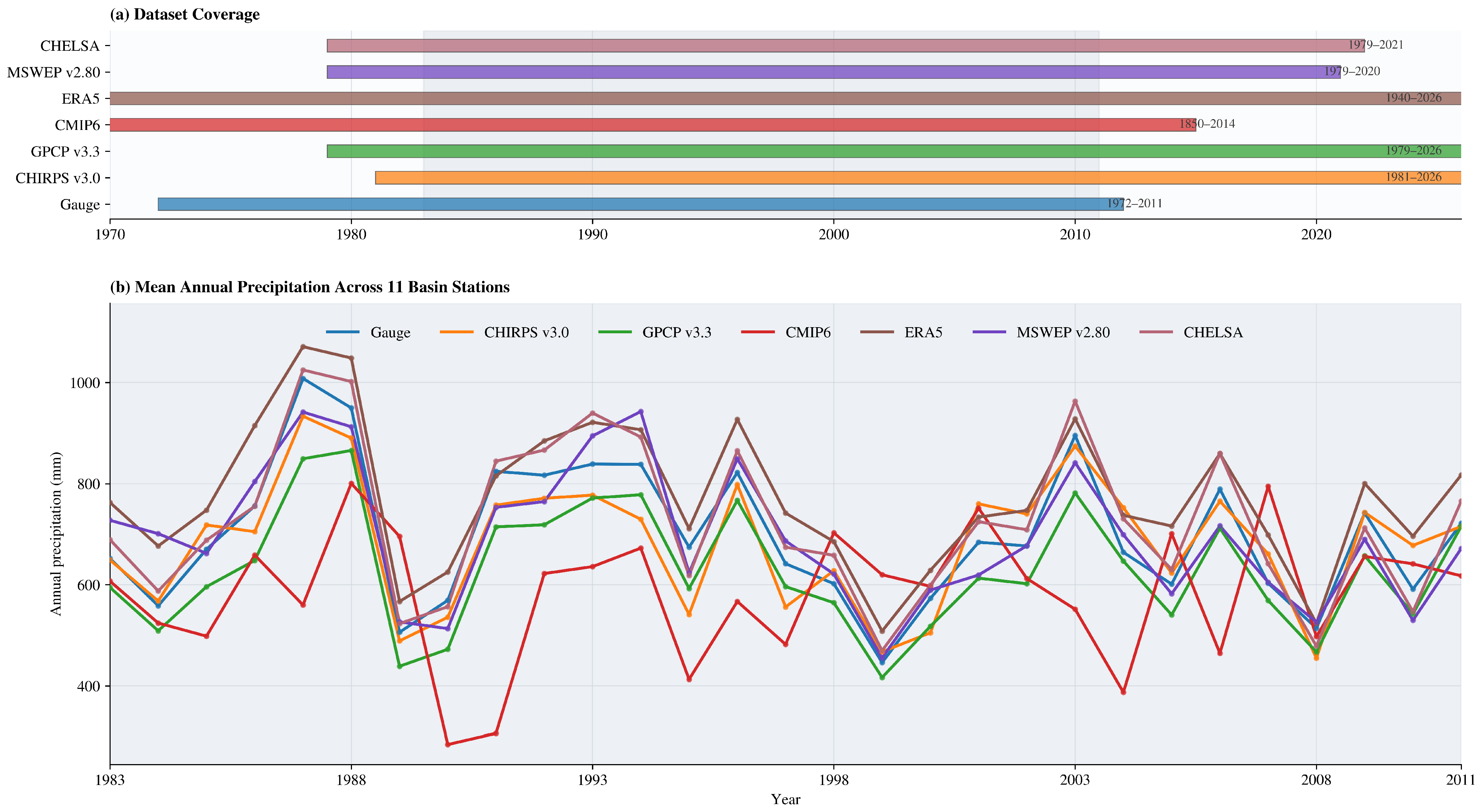
To ensure a consistent basis for inter-dataset evaluation, all precipitation datasets were assessed within a harmonized monthly comparison framework. Since the datasets differ in spatial resolution, temporal coverage, and data-generation approach, the final analysis was restricted to 1983–2011, corresponding to the common period shared by the gauge observations and all gridded datasets considered in this study. The dataset-specific spatial resolutions and archive periods are summarized in Table 1. The evaluation focused on directional class consistency rather than precipitation magnitude. Specifically, each precipitation dataset was assessed according to its ability to reproduce the dry, normal, and wet monthly classes derived from gauge observations. The main dataset characteristics are provided in Table 1, and Figure 2 shows the temporal coverage of the datasets together with the mean annual precipitation averaged across the basin gauge locations for the common comparison period.

2.3. The Classical Error Metrics

Although BERA formed the main analytical framework of this study, three conventional error metrics were also calculated for the common period 1983–2011 to provide a familiar baseline for comparison. These metrics quantify the agreement between gauge observations and the corresponding collocated precipitation dataset values in terms of magnitude, temporal correspondence, and systematic bias. They were therefore used as a complementary assessment to the class-based BERA results.
The Root Mean Square Error (RMSE) was used to measure the average deviation between the gauge observations and each precipitation dataset. Because it gives greater weight to large errors, RMSE is particularly sensitive to discrepancies during wet months and high-precipitation periods.
R M S E d = 1 n t = 1 n P d , t P g , t 2
where P d , t is the precipitation product value from dataset d at time t, P g , t is the corresponding gauge observation, and n is the total number of paired observations. Lower RMSE values indicate closer agreement with the gauge observations.
The coefficient of determination ( R 2 ) was used to quantify the strength of the linear relationship between the monthly precipitation values of the gauge observations and those of each evaluated dataset. In this study, R 2 was calculated as the square of the Pearson correlation coefficient between the gauge series and the dataset series.
R 2 = t = 1 n P g , t P ¯ g P d , t P ¯ d t = 1 n P g , t P ¯ g 2 t = 1 n P d , t P ¯ d 2 2
where P g and P d denote the mean precipitation values of the gauge observations and precipitation product dataset d, respectively. The value of R 2 ranges from 0 to 1, with higher values indicating stronger linear correspondence between the temporal variability of the dataset and the gauge record.
To assess the tendency of each dataset to systematically overestimate or underestimate precipitation relative to the gauge observations, the mean bias was calculated as
B I A S = 1 n t = 1 n ( P d , t P g , t )
A positive bias indicates overestimation relative to the gauge observations, whereas a negative bias indicates underestimation. In contrast to RMSE, which reflects the overall magnitude of deviation, bias captures the direction of the mean error.

3. Demonstrative Application Area and Results

This section presents the UTRC as the application basin used to demonstrate the proposed framework and briefly summarizes the conventional continuous error metrics used to complement the BERA framework.

3.1. Upper Tigris River Catchment

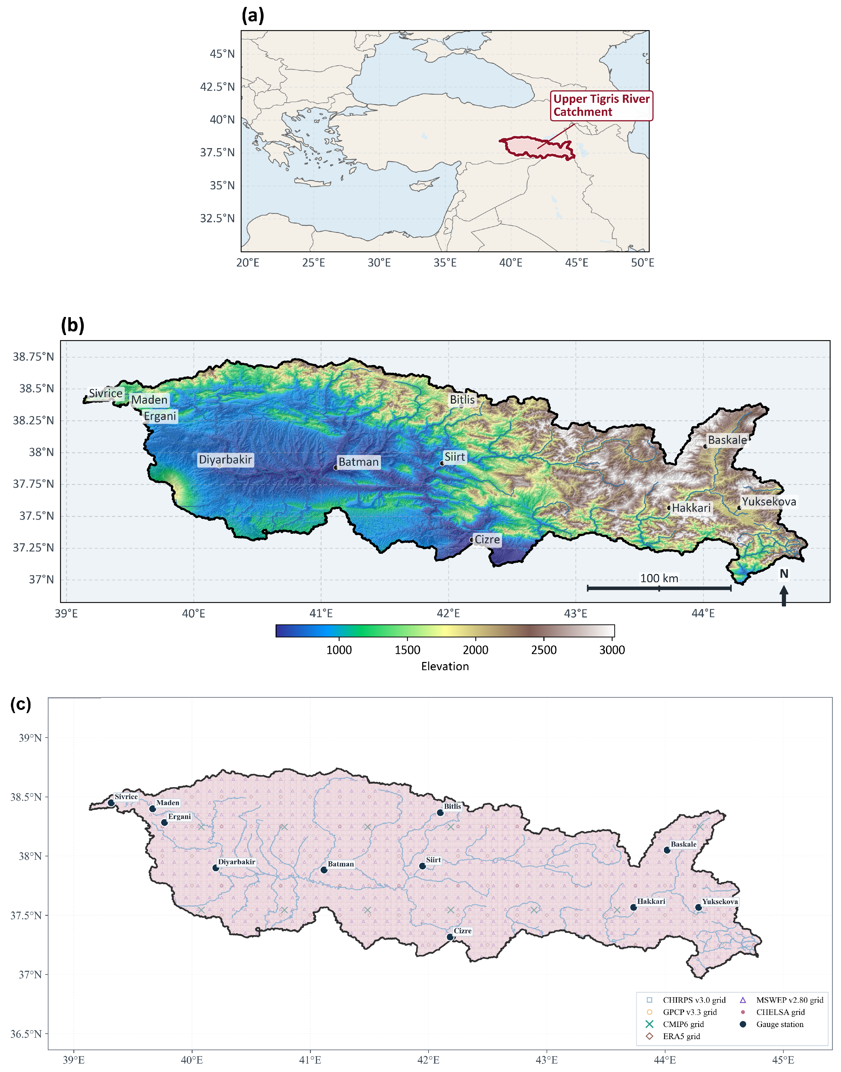
The UTRC is located in southeastern Türkiye and spans a pronounced west-to-east elevation gradient extending from the lower plains around Diyarbakir, Batman, and Cizre to the high mountain terrain of Bitlis, Hakkari, Baskale, and Yuksekova. This strong topographic contrast influences the drainage network, controls orographic precipitation, and produces substantial spatial variability in hydroclimatic conditions across the basin. Figure 3 illustrates the regional location of the basin together with the elevation structure, drainage pattern, and the selected gauge locations used in this application.
Monthly total gauge observations were obtained from the Turkish State Meteorological Service (TSMS) at 11 representative gauge locations: Hakkari, Yuksekova, Baskale, Siirt, Cizre, Batman, Diyarbakir, Bitlis, Ergani, Sivrice, and Maden, as shown in Figure 3b. These gauge locations were selected to represent the marked climatic and topographic contrasts of the UTRC and were used to evaluate the gridded precipitation products. Figure 3c shows the spatial arrangement of the gauge network together with the representative grid nodes used to sample the CHIRPS v3.0, GPCP v3.3, CMIP6, ERA5, MSWEP v2.80, and CHELSA products across the basin. This layout clarifies the spatial harmonization context of the comparison and highlights the differences between point-based gauge observations and the gridded precipitation products.
Before analysis, the monthly TSMS records were screened for missing entries, duplicate station–month keys, and negative precipitation values. The synchronized 1983–2011 record was complete at all eleven stations, so no statistical infilling was required. The homogeneity of each station record was further examined by applying the Pettitt and Standard Normal Homogeneity Test (SNHT) procedures to the annual totals [34,35]. Neither test detected a significant discontinuity at any station at the 5% level, indicating that the reference series contain no major non-climatic breaks over the study period.
Table 2 shows the marked contrast between the point support of the 11 TSMS gauges and the areal support of the product grids. A gauge accumulation and a grid-cell mean do not represent the same spatial quantity, even when their coordinates coincide; gauge uncertainty and point-to-pixel representativeness can therefore affect product evaluation [36]. The present analysis addresses spatial collocation only; it does not resolve this underlying support mismatch. Native product grids were preserved, and only the gridded fields were sampled at the gauge coordinates. This design avoids deliberately discarding the information contained in finer grids, but an 11-station comparison cannot quantify each product’s full spatial-field performance.
To sample the gridded fields at the gauge coordinates, radial basis function (RBF) interpolation was selected as the common collocation operator for all six products after comparison with nearest-neighbor, inverse-distance-weighting, and local-polynomial alternatives over the same stations and period. Candidate methods were evaluated with an equally weighted composite of normalized R 2 , RMSE, and absolute normalized bias. RBF yielded the highest mean composite score across the six products, although the best-scoring method differed among individual products. Its adoption therefore imposes a consistent collocation rule rather than implying that RBF is universally superior, a qualification consistent with studies showing that precipitation interpolation performance depends on network geometry, terrain, and climatic setting [37,38,39]. RBF was applied only to the gridded products and does not constitute downscaling: it estimates a value at a requested coordinate but does not create independently observed sub-grid precipitation structure.

3.2. Traditional Statistical Analyses

To complement the BERA framework, the demonstrative application includes conventional continuous error metrics calculated from the gauge-based monthly precipitation series. R 2 , R M S E , and B I A S are used to quantify the overall agreement between gauge observations and the evaluated precipitation products.
Table 3 summarizes the traditional error metric patterns between the gauge observations obtained from TSMS and the precipitation products for each station. As the table indicates, no single product dominates across all conventional performance dimensions: R 2 , bias, and Kendall’s τ emphasize different properties of the gauge–product relationship and consequently produce different station-level rankings. Any selection based on one of these metrics alone would therefore be criterion-dependent.
For example, CHELSA consistently exhibits the highest R 2 values across most stations, reaching 0.993 at Batman, 0.991 at Hakkari, and 0.987 at Siirt. Based on R 2 alone, CHELSA would appear to be the superior dataset. However, its bias values reveal substantial systematic errors, such as + 25.89 mm at Baskale, + 15.88 mm at Hakkari, and + 15.75 mm at Siirt. Moreover, despite the excellent R 2 performance, Kendall’s τ remains negative at all stations (e.g., 0.202 at Bitlis and 0.177 at Siirt), indicating a poor ability to reproduce the observed ranking or temporal variability of precipitation. A similar contradiction is observed for GPCP v3.3. This product achieves very high R 2 values, including 0.952 at Cizre and 0.979 at Hakkari, yet Kendall’s τ is negative at many stations (e.g., 0.117 at Bitlis and 0.093 at Siirt). Thus, strong variance agreement does not necessarily imply correct precipitation dynamics. Conversely, CHIRPS v3.0 generally presents lower R 2 values than CHELSA or GPCP but produces relatively small biases, such as 0.43 mm at Baskale and 1.20 mm at Hakkari. Nevertheless, its Kendall’s τ values remain close to zero, suggesting limited skill in capturing precipitation ordering.
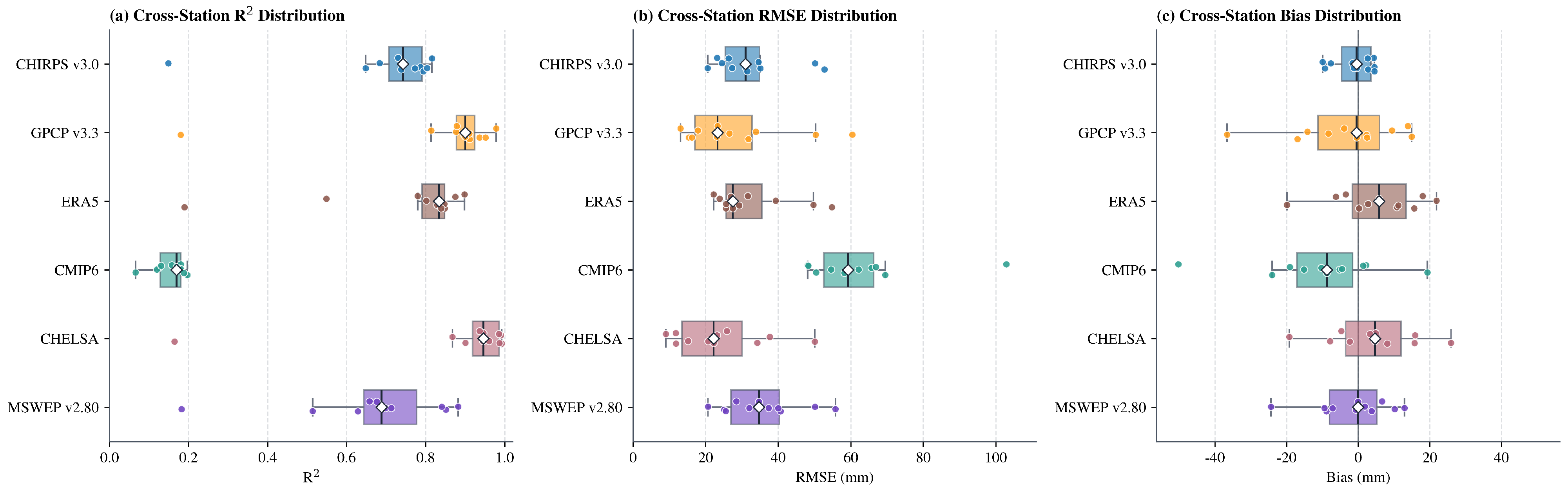
In addition, the cross-station metric distributions reveal a differentiated performance structure among the evaluated products. Figure 4 shows that CHIRPS v3.0 maintains one of the lowest bias tendencies together with a relatively constrained R M S E spread, whereas GPCP v3.3 and CHELSA exhibit stronger central R 2 behavior across stations. In contrast, CMIP6 remains more weakly aligned with the gauge record and displays a broader error structure. ERA5 and MSWEP occupy an intermediate position, indicating moderate but spatially variable continuous performance in the basin.
Both Table 3 and Figure 4 provide the conventional metric background in the UTRC application. These examples demonstrate that different metrics emphasize different aspects of performance. A product may explain variance well (high R 2 ), reproduce mean precipitation accurately (low bias), or preserve temporal structure (high Kendall’s τ ), but rarely all three simultaneously. Therefore, the statistics presented here are insufficient for unequivocal product selection, and the proposed BERA framework is required to identify the most suitable precipitation dataset.

3.3. Dataset-Level BERA Performance

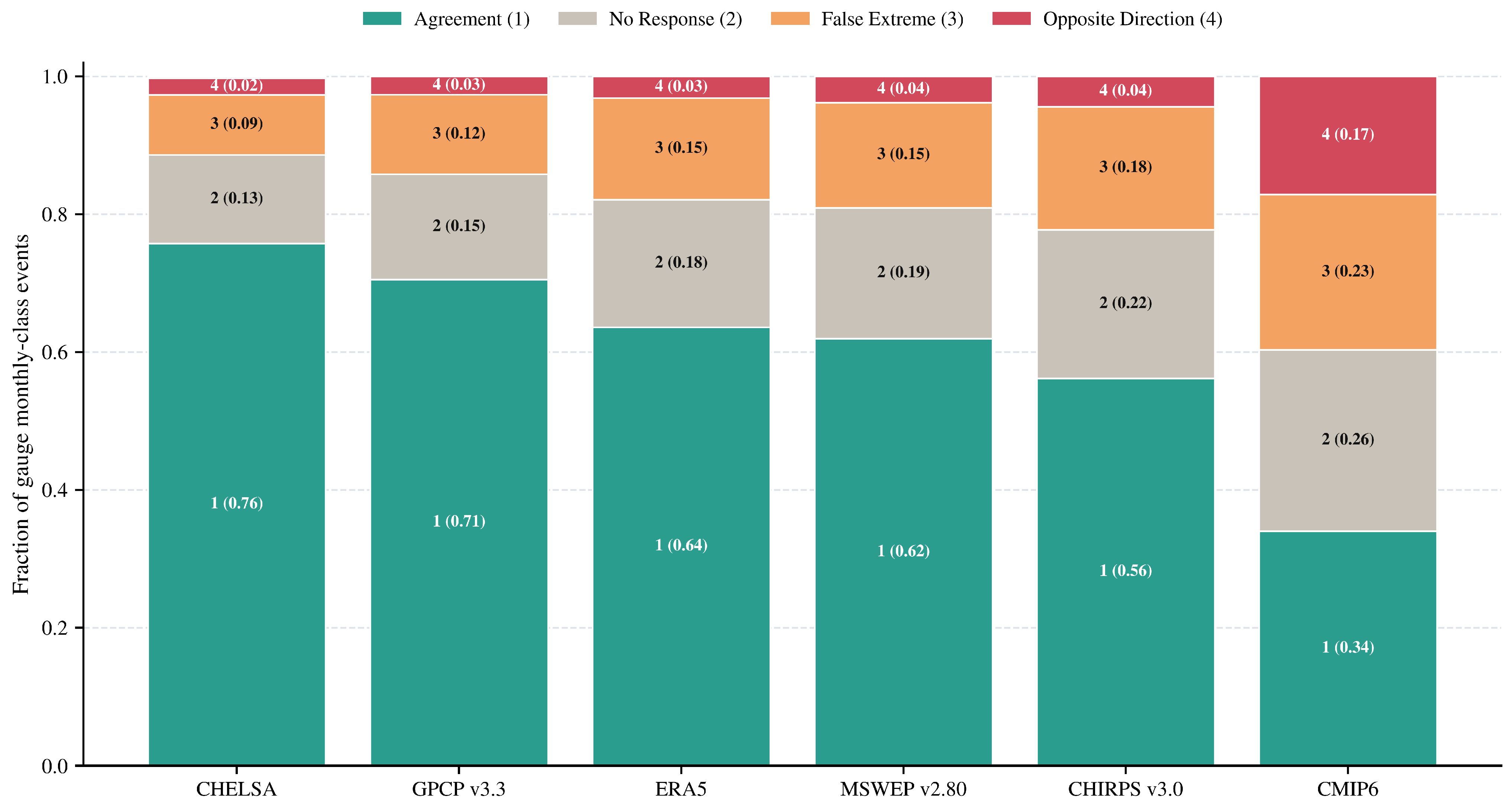
BERA was applied to each precipitation product. At the dataset level, agreement with the gauge-based monthly class structure varied widely across products. Figure 5 shows that CHELSA achieved the highest overall agreement rate (AR = 0.757), followed by GPCP v3.3 (AR = 0.705), whereas CMIP6 yielded the lowest agreement (AR = 0.340) and the largest share of opposite-direction responses. In practical terms, higher-performing products more frequently reproduced the observed monthly precipitation class assignments, while the weakest dataset more frequently shifted toward the wrong extreme. The agreement gap between the best and weakest products reached AR = 0.417, and the opposite-direction frequency of the weakest dataset (CMIP6) was 7.054 times larger than that of the strongest one (CHELSA). This distinction is scientifically important because no-response or false-extreme outcomes may still reflect partial event correspondence, whereas an opposite-direction response indicates that the dataset assigned to a particular month is the wrong side of the precipitation distribution altogether.
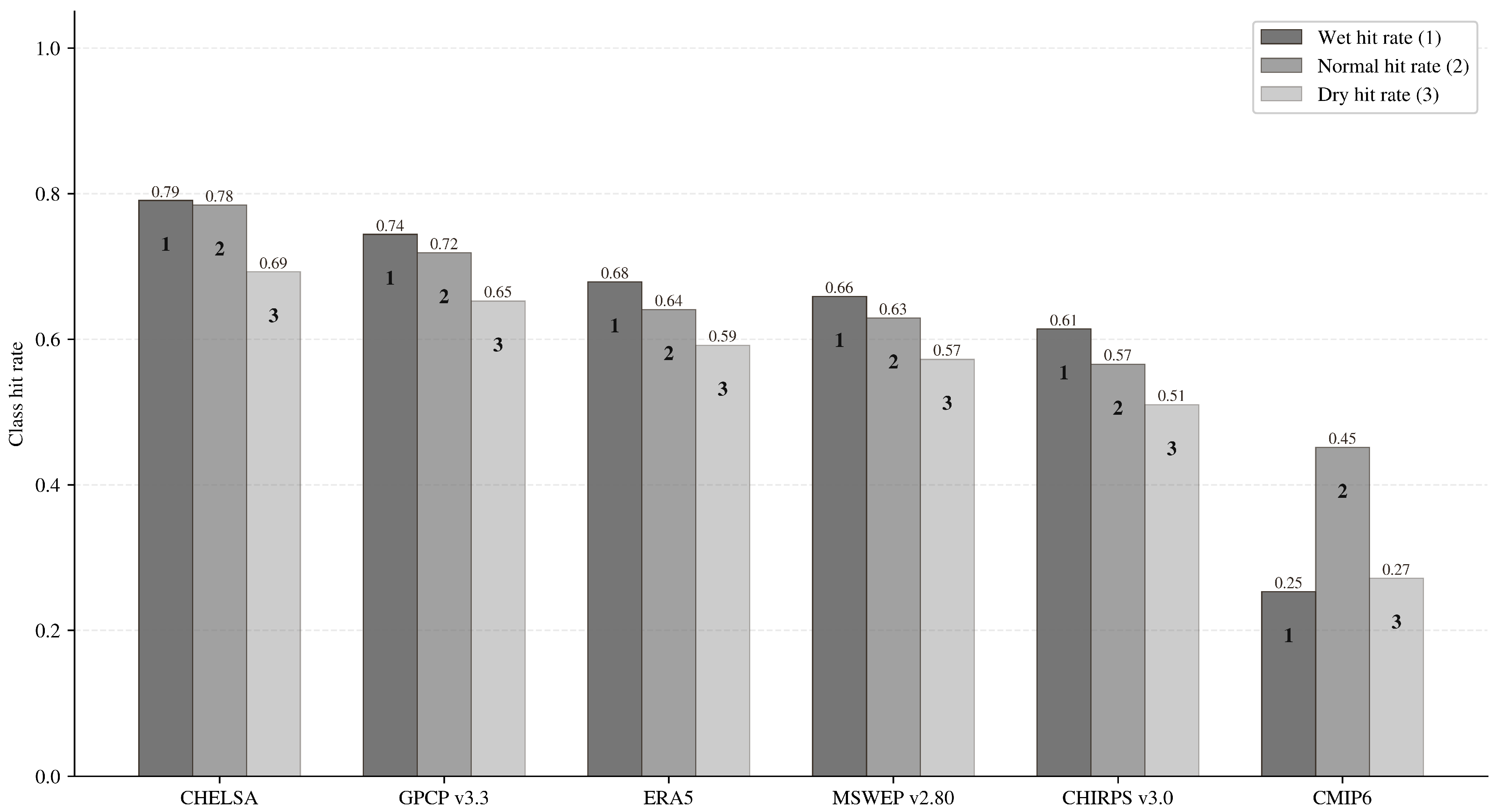
Class-specific hit rates further clarify the structure of this separation. Across five of the six products, wet-hit rates were higher than dry-hit rates, suggesting that positive monthly anomalies were reproduced more readily than dry anomalies. CHELSA showed the strongest class-specific response, with wet, dry, and normal H R = 0.791 , H R = 0.693 , and H R = 0.784 , respectively, whereas CMIP6 remained weak across all three classes ( H R = 0.253 wet, H R = 0.272 dry, and H R = 0.451 normal). Figure 6, therefore, shows that the main dataset separation emerged not only from overall agreement but also from the ability to preserve directional consistency across distinct monthly precipitation regimes. The wet-hit gap between the best and weakest products was 0.537, compared with 0.421 for dry months and 0.333 for normal months. In addition, CHIRPS v3.0 performed more favorably in the traditional metrics summarized in the previous section than in the BERA classification space, indicating that good continuous monthly skill does not automatically translate into reliable dry–wet class reproduction.

4. Discussion

This study set out to identify a suitable precipitation product for a given basin by examining the temporal precipitation distribution through a categorical classification. The results show that conventional performance metrics and BERA capture different dimensions of precipitation dataset behavior. As implemented in the preceding sections, the selection of precipitation products with the aggregate statistics did not necessarily preserve the observed directional structure of monthly anomalies. This differentiation is not a minor methodological detail. The dominant evaluation paradigm is still largely based on the correlation and bulk error metrics computed for the full record [5,7]. However, Maraun [20] argued that the evaluation based only on marginal or bulk agreement is insufficient for impact-oriented applications because it does not test whether or not a product reproduces the timing and sign of anomalous conditions. The BERA results support this argument by showing that a dataset may represent average precipitation behavior reasonably well, while still assigning individual months to an incorrect anomaly class. In this sense, the main contribution of this study is not simply to reorder a set of precipitation products over a basin, but to demonstrate that directional anomaly consistency constitutes an additional and necessary evaluation dimension. This point becomes particularly clear in the interpretation of the quality of CHIRPS. It has been widely adopted because of its strong performance in many conventional evaluations and its ability to reduce systematic magnitude bias through gauge-informed adjustment of a high-resolution infrared climatology [8]. However, the present analysis shows that low bias and relatively small continuous errors do not necessarily imply accurate reproduction of month-to-month anomaly direction. This distinction is consistent with a broader concern in the literature that temporal and event-specific representativeness cannot be inferred from bulk agreement alone. Herold et al. [18], for example, showed that products with comparable mean-state behavior may still diverge strongly in their representation of precipitation extremes. BERA extends this concern from the intensity domain into the anomaly-class domain by showing that the problem is not only whether extreme precipitation is too high or too low, but whether a month is assigned to the correct side of the local precipitation distribution at all. This shift in the evaluation perspective is important because the direction errors are qualitatively different from magnitude (or nominal) errors. A systematic bias can often be adjusted, but a month registered in the wrong anomaly class indicates a failure in temporal hydroclimatic interpretation.
BERA should therefore be positioned within, rather than outside, the established contingency-table literature. Its overall agreement is equivalent to three-class accuracy, and its class-specific hit rates correspond to class recall. POD, FAR, CSI, equitable scores, and spatial verification address related but distinct questions involving missed events, false alarms, event prevalence, chance agreement, or spatial displacement [21,22,23]. The contribution is diagnostic and interpretive: the off-diagonal cells are retained as no response, false extreme, and opposite direction so that hydroclimatically different failure pathways are not collapsed into one error total. BERA therefore complements established categorical measures; it neither replaces them nor introduces new contingency-table algebra.
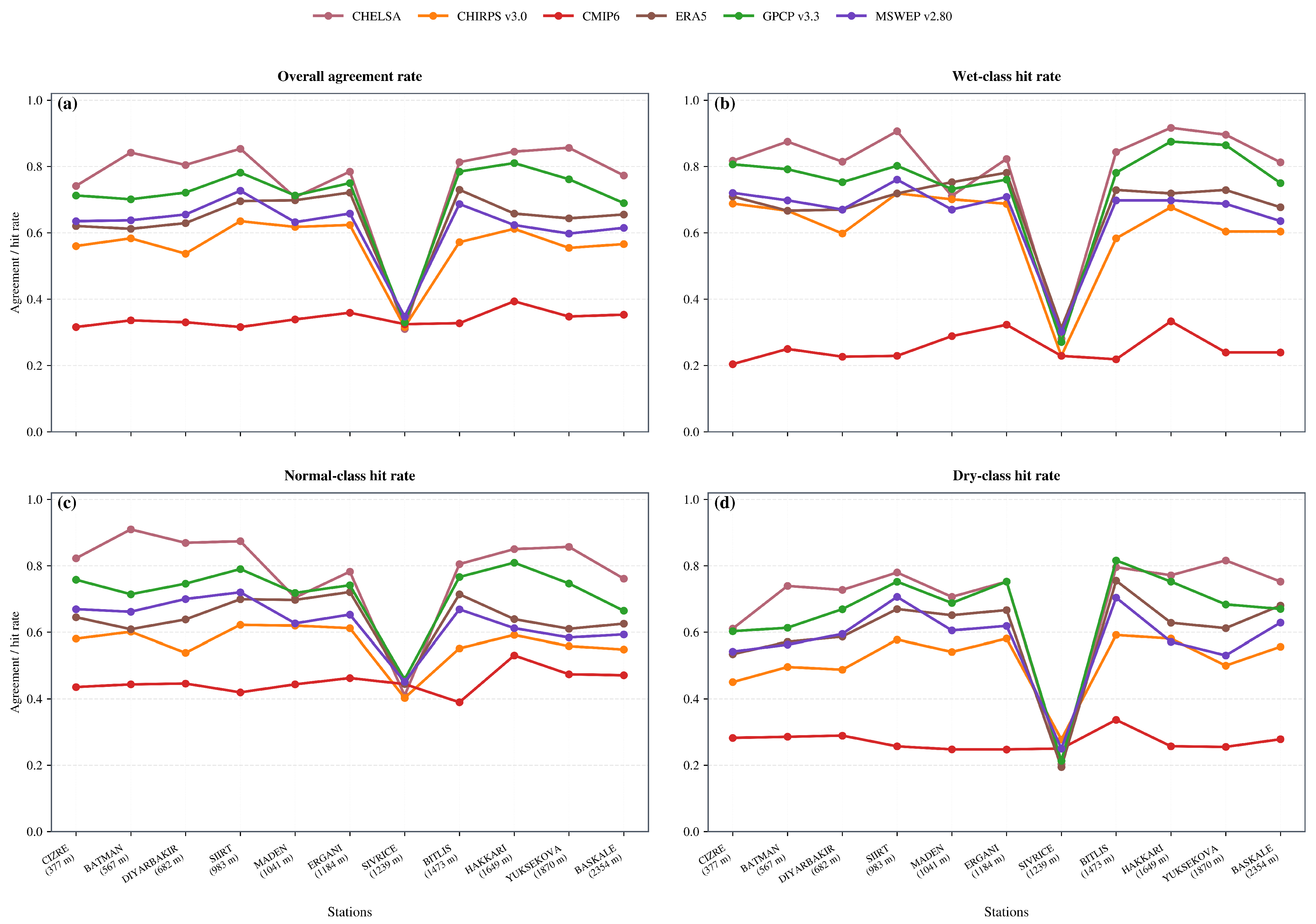
The station-level structure of these results deserves closer examination. Figure 7 resolves the dataset-level results by gauge, showing station-level profiles of overall agreement together with the wet-, normal-, and dry-class hit rates of each product. The most favorable station-average agreement rates occurred at Siirt ( A R = 0.668 ) and Hakkari ( A R = 0.657 ), whereas the clearest performance breakdown occurred at Sivrice ( A R = 0.327 ). The latter station was also characterized by high no-response ( C R = 0.269 ) and opposite-direction ( C R = 0.171 ) rates, indicating persistent difficulty in reproducing the observed month-to-month class shifts. CHELSA generally produced the highest agreement values across the stations, followed by GPCP v3.3. ERA5 and MSWEP v2.80 showed intermediate agreement, whereas CHIRPS v3.0 remained at moderate levels. CMIP6 exhibited the lowest agreement values for almost all stations, indicating weaker performance in reproducing the observed precipitation class behavior.
Because this weak performance appeared across all gridded products, it points to a local representativeness problem rather than a dataset-specific limitation. The homogeneity tests offer no support for a data-related explanation at this station: neither Pettitt’s test ( p = 0.899 ) nor SNHT ( p = 0.747 ) detected a discontinuity in the annual gauge series, although such tests cannot establish that the record is error-free. Since the deterioration appeared across products with different data-generation architectures, a failure specific to any single product is also unlikely to explain the shared pattern. Gauge–grid representativeness and microclimatic variability therefore remain the most plausible explanations, but the available observations cannot distinguish between them. Therefore, Figure 7 also highlights the need for station-level evaluation when using gridded precipitation datasets in extreme-class and drought-related analyses.
Overall, Figure 6 and Figure 7 show that the class-based ranking obtained at the dataset level was broadly reproduced at the individual stations. The station-level profiles further indicate that these product differences were amplified or damped by local hydroclimatic conditions, suggesting that regional dataset ranking and local reproducibility should be interpreted jointly rather than in isolation.
Considerable station-to-station variation nevertheless remained within every product, so this ordering summarizes the present basin, reference network, and comparison period; it should not be read as a context-independent ranking of product quality.
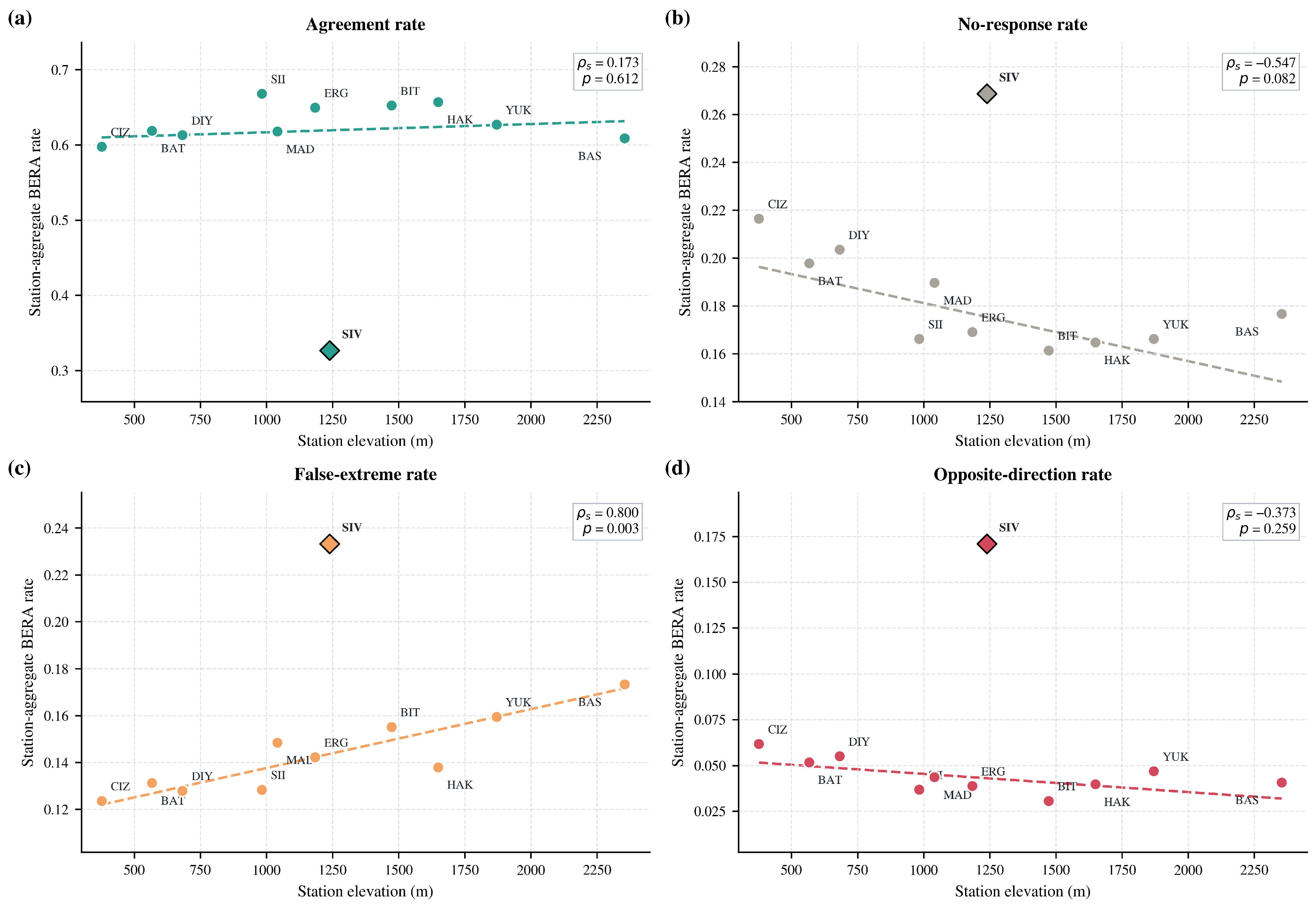
Topographic influence was evaluated by relating station elevation to the product-averaged agreement, no-response, false-extreme, and opposite-direction rates using four prespecified two-sided Spearman rank tests ( n = 11 ; Figure 8). The analysis found no evidence of a monotonic association with either agreement ( ρ s = 0.173 , p = 0.612 ) or opposite-direction rate ( ρ s = 0.373 , p = 0.259 ), while the negative association with no-response rate remained inconclusive ( ρ s = 0.547 , p = 0.082 ). False-extreme rate alone increased significantly with elevation ( ρ s = 0.800 , p = 0.003 ), satisfying both the nominal α = 0.05 criterion and the Bonferroni-adjusted benchmark of α = 0.0125 for four tests. The result therefore identifies an elevation-related increase in one specific error pathway—assigning an extreme class when the gauge month is normal—rather than a general deterioration of BERA performance with altitude. The Theil–Sen lines summarize trend direction and slope descriptively; statistical inference is based on the Spearman tests.
The stronger BERA performance of CHELSA and GPCP is therefore most meaningfully interpreted not as a generic statement of superiority, but as evidence that certain product designs are better aligned with directional anomaly reproduction. For CHELSA, this result is physically plausible because anomaly classification depends on the local climatological baseline, and a terrain-informed climatological structure is likely to be beneficial in a basin with strong elevation gradients and/or orographic controls. This interpretation is consistent with broader evidence that topographic complexity strongly conditions precipitation product performance and that products handling terrain effects more explicitly may gain an advantage in mountainous settings [7,14]. The recent Türkiye-wide assessment by Keserci [40] points in the same direction, particularly for complex terrain. GPCP, by contrast, appears to benefit from the long-established strength of gauge–satellite merging at monthly timescales [9], and the BERA results suggest that this strength extends beyond mean accumulation to the more demanding problem of anomaly-state correspondence. This interpretation is also compatible with the global comparison of Beck et al. [6], who showed the continued value of gauge-corrected merged products, although their evaluation framework did not isolate directional class consistency in the way BERA does.
These product characteristics offer plausible context for the results, not a causal explanation. Product family, native resolution, gauge adjustment, and spatial support vary together and cannot be disentangled in a single-basin station comparison. The observed ordering is therefore specific to the UTRC experiment and should not be generalized as an application-independent hierarchy.
ERA5 and MSWEP incorporate strong physical or multi-source design logic, yet the BERA results indicate that such integration does not automatically resolve directional classification error. This is important because both products are often treated as robust general-purpose inputs. MSWEP was explicitly developed to combine the complementary strengths of gauge, satellite, and reanalysis information [1,41], but the BERA results show that improved mean-state representation does not necessarily translate into consistent anomaly-state reproduction. ERA5 presents a similar issue from a different angle: physically coherent reanalysis output may still contain anomaly-direction distortions that are not obvious under conventional metrics. The findings of Abu Arra and Şişman [42], who showed that bias correction substantially altered ERA5-based drought characterization, support this interpretation. BERA is valuable here because it identifies precisely the type of weakness that remains partly hidden when evaluation is conducted via the conventional error metrics, including R 2 , RMSE, bias, or correlation. The poorest performance of raw CMIP6 output further clarifies why the BERA perspective matters. The weakness of raw climate model precipitation at the station scale is expected, but BERA shows that the problem is not merely one of biased magnitude or inadequate local calibration. It is also a problem of directional inconsistency, meaning that monthly anomalies are frequently assigned in the wrong class relative to observations. This is a more serious limitation for impact studies than a simple offset because it undermines the interpretability of anomalous wet and dry periods. Existing bias-correction literature has already shown that adjustments can improve statistical behavior while leaving structural limitations unresolved [11,43,44].
Interpretation of EC-Earth3 requires an additional qualification. CMIP6 simulations are free-running climate-model realizations designed to represent climate statistics and forced responses, not to reconstruct the observed chronology at individual stations [32,33]. Its low monthly BERA agreement therefore constrains direct use of the raw series for local anomaly monitoring; it does not assess the value of EC-Earth3 for climate-process studies or projections. Nor does the numerical similarity between the 12 model cells in the basin and the 11 gauges imply comparable sampling support: a model cell is an areal mean generated by resolved and parameterized processes, whereas a gauge is a point observation. Scale-appropriate evaluation, and often downscaling or bias adjustment, remains necessary before local impact use [11,43].
In the context of precipitation evaluation, the BERA results add an important diagnostic layer by demonstrating that post-correction assessment should not be limited to improvements in mean or variance agreement. Instead, it should also test whether gridded products can correctly reproduce the observed directional behavior of rainfall, particularly transitions between wet, normal, and dry classes. In this manner, BERA is not a replacement for correction methods, but a complementary verification tool for determining whether such methods improve the aspects of performance that are most relevant to anomaly-based applications.
Another important outcome is the asymmetry between wet and dry anomaly reproduction. Across most products, wet-class hit rates exceeded dry-class hit rates, indicating that negative monthly anomalies were generally harder to reproduce than positive ones. This pattern is methodologically significant because it shows that directional skill is not uniform across the precipitation distribution. The literature on precipitation extremes has mostly emphasized the uncertainty toward the upper tail [18], but the BERA framework indicates that the lower tail may be more problematic when the goal is to identify dry anomaly states correctly. This has direct practical implications. In regions where water management depends heavily on the correct recognition of precipitation deficits, a product with acceptable standard error metrics is unreliable for drought-oriented interpretation. This concern aligns with the broader climate-risk context of the Eastern Mediterranean and Middle East, where increasing hydroclimatic stress heightens the importance of correctly identifying both anomalously wet and anomalously dry periods [28]. It also suggests that BERA is especially relevant for the applications connected to drought early warning and anomaly-sensitive water assessment, where a false directional classification may have greater practical consequences than a moderate magnitude error.
Several mechanisms can contribute to this behavior, although they differ among product families. Infrared methods infer rainfall indirectly from cloud-top properties, while passive-microwave retrievals sample intermittently and may miss light or warm precipitation [45,46,47]. CHIRPS combines infrared cold-cloud-duration estimates with gauges [8]; reanalysis, climatological, and climate-model products introduce different effects through model physics, temporal aggregation, and spatial support. At monthly scale, small positive errors or spatial averaging can shift a gauge-defined dry month into the normal class. These mechanisms make the observed asymmetry plausible, but the present multi-product experiment cannot attribute it to a single retrieval or modelling process.
The station-scale variation in BERA performance further suggests that the directional class agreement contains meaningful spatial structure rather than random classification noise. Since all products were harmonized to station locations using the same interpolation method, the remaining station-to-station differences are more likely to reflect local representativeness, terrain-related precipitation variability, or gauge–grid mismatch than to inconsistencies in the spatial matching method. This interpretation is consistent with studies showing that product performance is strongly modulated by local terrain, climatic transition zones, and the representativeness of gridded fields relative to point observations [7,14]. In other words, BERA does not merely reproduce what conventional statistics already indicate; it reveals where anomaly-direction agreement breaks down spatially and therefore where hydroclimatic interpretation should be treated with greater caution.
Some caution is nevertheless required regarding the spatial-matching design itself. Using a single RBF procedure places all products at the same sampling coordinates, but it neither makes a point observation equivalent to a grid-cell mean nor removes interpolation uncertainty [36]. Repeating the complete q 25 / q 75 analysis with nearest-cell extraction preserved the product ordering, with the largest absolute change in agreement being 0.011 and the largest change in any response fraction being 0.033. This sensitivity check supports stability for the two operators tested, although it does not cover all spatial-matching or terrain-aware alternatives. The elevation analysis presented above calls for a similarly specific reading: elevation was associated with the false-extreme pathway alone, not with a general decline in BERA performance.
Conventional metrics remain necessary for quantifying overall agreement, but they are insufficient when the scientific or operational question depends on whether a dataset correctly reproduces the sign and class of monthly anomalies. The present study therefore reinforces a broader methodological lesson emerging from the precipitation evaluation literature: product choice should be application-specific, but application specificity cannot be defined only in terms of mean error or temporal correlation [5,6,7]. For anomaly-sensitive applications, an additional layer of class-resolved evaluation is required. BERA provides that layer in a simple station-based form and shows that some products that appear reliable under standard verification may still be inadequate for anomaly-state interpretation. The framework nevertheless has limits. It was applied here at a monthly timescale, over a finite common period, and with internally defined percentile thresholds that isolate directional agreement rather than absolute threshold accuracy. These are appropriate design choices for the present objective, but they also indicate the next step: testing whether the same diagnostic separation between conventional agreement and directional anomaly consistency persists across daily timescales, additional climatic regions, and bias-corrected model products. Even with these limitations, the main implication is clear: evaluating precipitation datasets without explicitly testing directional anomaly reproduction risks overstating their practical reliability.
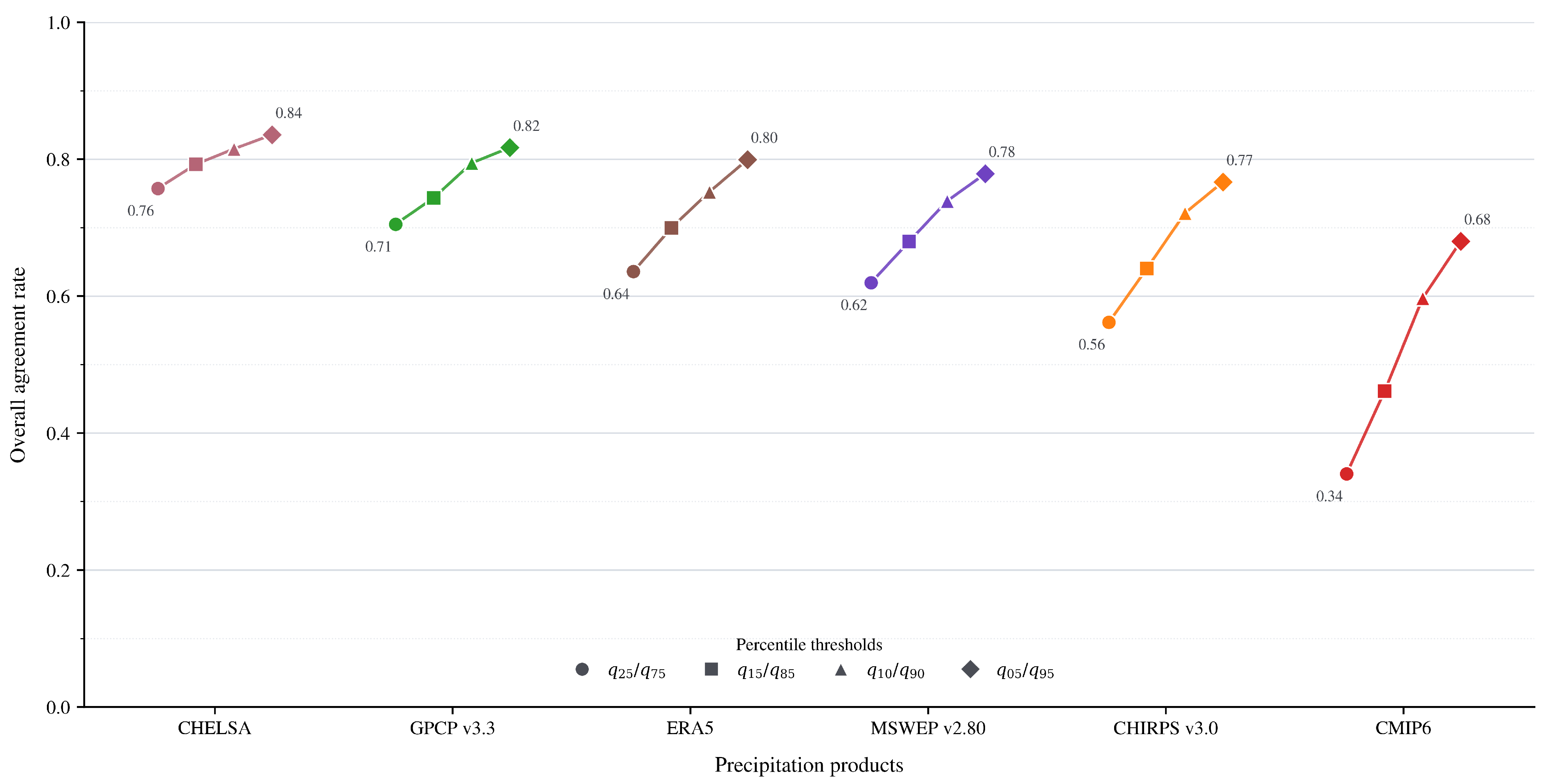
The threshold experiment summarized in Figure 9 makes this trade-off explicit by separating rank stability from score composition. The ordering of the six products remained unchanged under all four threshold pairs (CHELSA > GPCP v3.3 > ERA5 > MSWEP v2.80 > CHIRPS v3.0 > CMIP6), indicating that the comparative ranking was robust within the tested range. The upward shift in overall agreement under stricter thresholds must not, however, be interpreted as improved detection of extreme months. Overall agreement is the raw fraction of the 3828 station–month pairs that fall on the diagonal of the three-class table and is therefore influenced by class prevalence. Moving from q 25 / q 75 to q 05 / q 95 expands the central interval used to define the normal class in both the gauge and product series. Gauge normal-class prevalence consequently increased from 0.411 to 0.776, while the number of gauge dry-plus-wet events declined from 2255 to 857, a reduction of 62.0%. Across the six products, the mean normal-class hit rate increased from 0.632 to 0.916, whereas the mean wet- and dry-class hit rates decreased from 0.623 to 0.434 and from 0.548 to 0.249, respectively. Thus, the higher overall agreement at stricter thresholds primarily reflects more frequent normal–normal matches and weaker tail support, rather than stronger extreme-class skill. The q 25 / q 75 definition was retained because it preserved the same product ordering while supplying substantially more dry and wet observations for class-specific estimation; it is a sample-support choice for this 29-year record, not a universal drought or wetness threshold.
The 1983–2011 interval is the longest period shared by the TSMS observations and all six products, and the reference network is consequently limited to the 11 TSMS gauges with complete monthly records over that interval. Holding the reference period and station set constant gives every product the same sample support and climatological window, but it constrains temporal coverage and network density. The present evidence should therefore be read as a regional proof of concept for the diagnostic behavior of BERA, not as empirical validation across climates and observing systems. Establishing broader robustness will require independent tests with denser networks, longer records, additional basins, and daily as well as monthly data.

5. Conclusions

This study proposed and applied the Bidirectional Extreme Response Analysis (BERA) framework to evaluate whether different precipitation datasets can reproduce the observed directional behavior of monthly precipitation anomalies. Unlike conventional metrics that mainly quantify magnitude agreement, BERA assesses whether a dataset correctly reproduces the observed monthly hydroclimatic state as wet, normal, or dry. The framework was then benchmarked in the Upper Tigris River Catchment (UTRC) using multiple precipitation products representing different data-generation approaches. The main conclusions of the study are summarized as follows:
  • The results demonstrate that precipitation dataset performance is strongly shaped by the scale, objective, and hydroclimatic context of their intended application. Therefore, the evaluated products should not be interpreted as directly interchangeable alternatives. Rather, they represent different data-generation paradigms, including satellite-based retrieval, satellite–gauge merging, reanalysis-based, multi-source integration, terrain-informed climatology, and climate-model-derived products. Their strengths and limitations should therefore be interpreted in relation to these methodological characteristics and intended uses, rather than through a single universal ranking.
  • CHELSA and GPCP v3.3 showed the strongest ability to preserve the observed monthly wet–normal–dry class structure in the UTRC. The relatively high BERA performance of CHELSA is scientifically meaningful because the basin is characterized by strong topographic gradients and orographic precipitation controls. Its terrain-informed climatological structure may have contributed to the better representation of gauge-based anomaly classes under complex terrain conditions. GPCP v3.3 also provided strong directional agreement, suggesting that satellite–gauge merging at monthly timescales can support not only general precipitation estimation but also the reproduction of hydroclimatic anomaly states.
  • ERA5 and MSWEP v2.80 occupied an intermediate position. Their results indicate that physically consistent reanalysis products and multi-source merged datasets can provide useful regional-scale precipitation information, but their ability to reproduce local monthly anomaly classes remains spatially variable. These products may therefore be suitable for broader hydroclimatic assessments, model forcing, or comparative regional analyses, but they should still be locally evaluated before being used for drought classification, station-scale anomaly detection, or decision-oriented water-resource applications.
  • The performance of CHIRPS v3.0 should be interpreted with particular attention to the distinction between continuous-metric skill and class-based anomaly reproduction. Although it is often preferred because of its high spatial resolution, gauge-informed structure, and generally favorable performance in many hydrological studies, the present BERA results show that good continuous performance does not necessarily guarantee correct dry–wet class reproduction. This does not imply that CHIRPS is an unsuitable precipitation product. Rather, it indicates that CHIRPS may be more reliable for applications focused on precipitation magnitude, spatial rainfall patterns, or broad hydroclimatic variability than for applications requiring strict month-to-month anomaly-class agreement at the station scale. Therefore, CHIRPS should be evaluated according to the specific objective of the study rather than dismissed based on class-based results alone.
  • CMIP6 EC-Earth3 exhibited the weakest BERA performance among the evaluated datasets, especially in reproducing station-scale monthly anomaly classes. However, this result should not be interpreted as an inherent limitation of CMIP6 as a climate modelling framework. Unlike the other products, CMIP6 is not an observational reconstruction or a gauge-adjusted precipitation estimate; it is a climate-model-derived dataset designed primarily for climate diagnostics, scenario analysis, and future projection studies. Therefore, its lower local agreement is expected when it is compared directly with station observations at monthly scale. The value of CMIP6 lies not in reproducing exact local precipitation classes, but in providing physically consistent simulations of large-scale climate variability and future hydroclimatic change. In this respect, CMIP6 remains essential for regional climate-impact assessments and projection-based studies, although its direct use for local drought classification or station-scale water-management decisions should require downscaling, bias correction, and additional validation.
  • A key implication of this study is that precipitation product selection should be guided by the intended application rather than by a single performance ranking. For local anomaly monitoring and drought classification, products with stronger directional agreement, such as CHELSA and GPCP v3.3, may be more appropriate. For regional hydroclimatic forcing or physically consistent atmospheric interpretation, ERA5 and MSWEP v2.80 may remain useful. For high-resolution satellite-based rainfall monitoring, CHIRPS continues to provide practical value, but its anomaly-class behavior should be independently tested. For future climate-risk assessment, CMIP6 is indispensable despite its lower station-scale BERA performance, because it is the only product category capable of providing scenario-based projection information.
  • No monotonic decline in overall BERA agreement with station elevation was detected. False-extreme rate, however, showed a positive rank association with elevation. The topographic signal was therefore confined to one disagreement pathway rather than expressed as a uniform change in the station ranking.
  • Owing to its flexible structure, BERA can be adapted to more detailed or application-specific classification schemes. This allows agreement and disagreement patterns to be interpreted according to the purpose and criticality of the intended application, rather than being limited to a fixed statistical definition of product performance.
Overall, BERA provides an interpretable decomposition of a three-class contingency table rather than a replacement for established verification methods. Reporting no response, false extreme, and opposite direction alongside class-specific hit rates preserves distinctions that disappear when performance is reduced to a single summary score. In the UTRC, this decomposition changed the interpretation of several products and revealed an elevation-related pattern in the false-extreme pathway. The procedure can be applied wherever defensible reference classes are available, but the empirical findings reported here remain conditional on the basin, station network, common period, thresholds, and spatial-matching design.

Author Contributions

Conceptualization, A.U.Ş. and C.D.; methodology, A.U.Ş.; formal analysis, C.D.; investigation, C.D. and A.Ö.; data curation, C.D. and A.Ö.; writing—original draft preparation, A.U.Ş., C.D. and A.Ö.; writing—review and editing, A.U.Ş., C.D. and A.Ö. All authors have read and agreed to the published version of the manuscript.

Funding

This research received no external funding.

Institutional Review Board Statement

Not applicable.

Informed Consent Statement

Not applicable.

Data Availability Statement

All gridded precipitation datasets analysed in this study are openly available from their original providers: CHIRPS v3.0 (https://www.chc.ucsb.edu/data/chirps3 (accessed on 3 August 2026)); GPCP v3.3 (https://disc.gsfc.nasa.gov/datasets/GPCPMON_3.3/summary (accessed on 3 August 2026)); ERA5 (https://cds.climate.copernicus.eu); MSWEP v2.80 (https://www.gloh2o.org/mswep (accessed on 3 August 2026)); CHELSA (https://chelsa-climate.org); and CMIP6 EC-Earth3 (Copernicus Climate Data Store, https://cds.climate.copernicus.eu). The monthly gauge observations are licensed data of the Turkish State Meteorological Service (TSMS, https://www.mgm.gov.tr); they were obtained under licence for this study and are not publicly redistributable, but can be requested directly from TSMS. The derived datasets generated during the analysis are available from the corresponding author upon reasonable request.

Acknowledgments

C.D., A.Ö. and A.U.Ş. thank the Turkish State Meteorological Service for providing the precipitation dataset of the Upper Tigris River Catchment. During the preparation of this manuscript, the author(s) used ChatGPT v.5 for the purposes of English proofreading. The authors have reviewed and edited the output and take full responsibility for the content of this publication.

Conflicts of Interest

The authors declare no conflicts of interest.

Abbreviations

The following abbreviations are used in this manuscript:
ARAgreement Rate
BERABidirectional Extreme Response Analysis
CHELSAClimatologies at High Resolution for the Earth’s Land Surface Areas
CHIRPS  Climate Hazards Group InfraRed Precipitation with Station data
CMIP6Coupled Model Intercomparison Project Phase 6
CSICritical Success Index
ERA5European Centre for Medium-Range Weather Forecasts reanalysis
FARFalse Alarm Ratio
FERFalse-Extreme Rate
GPCPGlobal Precipitation Climatology Project
MSWEPMulti-Source Weighted-Ensemble Precipitation
NRRNo-Response Rate
ODROpposite-Direction Rate
PODProbability of Detection
RBFRadial Basis Function
RMSERoot Mean Squared Error
SNHTStandard Normal Homogeneity Test
TSMSTurkish State Meteorological Service
UTRCUpper Tigris River Catchment

References

  1. Beck, H.E.; van Dijk, A.I.J.M.; Levizzani, V.; Schellekens, J.; Miralles, D.G.; Martens, B.; de Roo, A. MSWEP: 3-hourly 0.25 global gridded precipitation (1979–2015) by merging gauge, satellite, and reanalysis data. Hydrol. Earth Syst. Sci. 2017, 21, 589–615. [Google Scholar] [CrossRef]
  2. Abdallah, M.; Zhang, K.; Chao, L.; Omer, A.; Hassaballah, K.; Welde Reda, K.; Liu, L.; Tola, T.L.; Nour, O.M. A D-vine copula-based quantile regression towards merging satellite precipitation products over rugged topography: A case study in the upper Tekeze–Atbara Basin. Hydrol. Earth Syst. Sci. 2024, 28, 1147–1174. [Google Scholar] [CrossRef]
  3. Ning, S.; Cheng, Y.; Zhou, Y.; Wang, J.; Zhang, Y.; Jin, J.; Thapa, B.R. Bayesian Model Averaging for Satellite Precipitation Data Fusion: From Accuracy Estimation to Runoff Simulation. Remote Sens. 2025, 17, 1154. [Google Scholar] [CrossRef]
  4. Tan, A.; Li, M.; Liu, H.; Chen, L.; Wang, T.; Wang, W.; Shi, Y. Comparative Assessment of Eight Satellite Precipitation Products over the Complex Terrain of the Lower Yarlung Zangpo Basin: Performance Evaluation and Topographic Influence Analysis. Remote Sens. 2025, 18, 63. [Google Scholar] [CrossRef]
  5. Sun, Q.; Miao, C.; Duan, Q.; Ashouri, H.; Sorooshian, S.; Hsu, K. A review of global precipitation data sets: Data sources, estimation, and intercomparisons. Rev. Geophys. 2017, 56, 79–107. [Google Scholar] [CrossRef]
  6. Beck, H.E.; Vergopolan, N.; Pan, M.; Levizzani, V.; van Dijk, A.I.J.M.; Weedon, G.P.; Brocca, L.; Pappenberger, F.; Huffman, G.J.; Wood, E.F. Global-scale evaluation of 22 precipitation datasets using gauge observations and hydrological modeling. Hydrol. Earth Syst. Sci. 2017, 21, 6201–6217. [Google Scholar] [CrossRef]
  7. Mankin, K.R.; Mehan, S.; Green, T.R.; Barnard, D.M. Review of gridded climate products and their use in hydrological analyses reveals overlaps, gaps, and the need for a more objective approach to selecting model forcing datasets. Hydrol. Earth Syst. Sci. 2025, 29, 85–117. [Google Scholar] [CrossRef]
  8. Funk, C.; Peterson, P.; Landsfeld, M.; Pedreros, D.; Verdin, J.; Shukla, S.; Husak, G.; Rowland, J.; Harrison, L.; Hoell, A.; et al. The climate hazards infrared precipitation with stations—A new environmental record for monitoring extremes. Sci. Data 2015, 2, 150066. [Google Scholar] [CrossRef] [PubMed]
  9. Huffman, G.J.; Adler, R.F.; Arkin, P.A.; Chang, A.T.C.; Ferraro, R.; Gruber, A.; Janowiak, J.E.; McNab, A.; Rudolf, B.; Schneider, U. The Global Precipitation Climatology Project (GPCP) combined precipitation dataset. Bull. Am. Meteorol. Soc. 1997, 78, 5–20. [Google Scholar] [CrossRef]
  10. Hersbach, H.; Bell, B.; Berrisford, P.; Hirahara, S.; Horányi, A.; Muñoz-Sabater, J.; Nicolas, J.; Peubey, C.; Radu, R.; Schepers, D.; et al. The ERA5 global reanalysis. Q. J. R. Meteorol. Soc. 2020, 146, 1999–2049. [Google Scholar] [CrossRef]
  11. Chinasho, A. Performance evaluation of bias correction methods for CMIP6 precipitation datasets in the drylands of the Wolaita Zone, Southern Ethiopia. Int. J. Clim. Change Strateg. Manag. 2025, 17, 1119–1139. [Google Scholar] [CrossRef]
  12. Goudiaby, O.; Bodian, A.; Dezetter, A.; Diouf, I.; Ogilvie, A. Evaluation of gridded rainfall products in three West African basins. Hydrology 2024, 11, 75. [Google Scholar] [CrossRef]
  13. Gacu, J.G.; Kantoush, S.; Nguyen, B.Q. Full-cycle evaluation of multi-source precipitation products for hydrological applications in the Magat River Basin, Philippines. Remote Sens. 2025, 17, 3375. [Google Scholar] [CrossRef]
  14. Nasimi, M.N.; Bauer-Gottwein, P.; Boyce, S.E.; Huang, J.; Disse, M. Gridded precipitation and temperature products performance over Afghanistan: From simple bias correction to advanced data fusion. Int. J. Remote Sens. 2025, 46. [Google Scholar] [CrossRef]
  15. Kassem, Y.; Gökçekuş, H.; Alijl, N. Gridded precipitation datasets and gauge precipitation products for driving hydrological models in the Dead Sea Region, Jordan. Sustainability 2023, 15, 11965. [Google Scholar] [CrossRef]
  16. Quichimbo, E.A.; Singer, M.; Michaelides, K.; Rosolem, R.; MacLeod, D.; Asfaw, D.T.; Cuthbert, M. Assessing the sensitivity of modelled water partitioning to global precipitation datasets in a data-scarce dryland region. Hydrol. Process. 2023, 37, e15047. [Google Scholar] [CrossRef]
  17. Rudiantoro, G.; Khomsin; Giarno. Comparison of the performance of four bias correction methods for Climate Hazards Group InfraRed Precipitation with Station Data (CHIRPS) in Sumatra. IOP Conf. Ser. Earth Environ. Sci. 2025, 1551, 012039. [Google Scholar] [CrossRef]
  18. Herold, N.; Behrangi, A.; Alexander, L.V. Large uncertainties in observed daily precipitation extremes over land. J. Geophys. Res. Atmos. 2016, 121, 14588–14608. [Google Scholar] [CrossRef]
  19. Katsanos, D.; Retalis, A.; Kalogiros, J.; Psiloglou, B.E.; Roukounakis, N.; Anagnostou, M. Performance evaluation of satellite precipitation products during extreme events—The case of the Medicane Daniel in Thessaly, Greece. Remote Sens. 2024, 16, 4216. [Google Scholar] [CrossRef]
  20. Maraun, D. Bias correcting climate change simulations—A critical review. Curr. Clim. Change Rep. 2016, 2, 211–220. [Google Scholar] [CrossRef]
  21. Jolliffe, I.T.; Stephenson, D.B. (Eds.) Forecast Verification: A Practitioner’s Guide in Atmospheric Science, 2nd ed.; John Wiley & Sons: Chichester, UK, 2012. [Google Scholar]
  22. Ebert, E.E. Fuzzy verification of high-resolution gridded forecasts: A review and proposed framework. Meteorol. Appl. 2008, 15, 51–64. [Google Scholar] [CrossRef]
  23. Gilleland, E.; Ahijevych, D.; Brown, B.G.; Casati, B.; Ebert, E.E. Intercomparison of spatial forecast verification methods. Weather Forecast. 2009, 24, 1416–1430. [Google Scholar] [CrossRef]
  24. Roberts, N.M.; Lean, H.W. Scale-selective verification of rainfall accumulations from high-resolution forecasts of convective events. Mon. Weather Rev. 2008, 136, 78–97. [Google Scholar] [CrossRef]
  25. Roebber, P.J. Visualizing multiple measures of forecast quality. Weather Forecast. 2009, 24, 601–608. [Google Scholar] [CrossRef]
  26. Ferro, C.A.T.; Stephenson, D.B. Extremal dependence indices: Improved verification measures for deterministic forecasts of rare binary events. Weather Forecast. 2011, 26, 699–713. [Google Scholar] [CrossRef]
  27. Gandin, L.S.; Murphy, A.H. Equitable skill scores for categorical forecasts. Mon. Weather Rev. 1992, 120, 361–370. [Google Scholar] [CrossRef]
  28. Zittis, G.; Almazroui, M.; Alpert, P.; Ciais, P.; Cramer, W.; Dahdal, Y.; Fnais, M.S.; Francis, D.; Hadjinicolaou, P.; Howari, F.M.; et al. Climate change and weather extremes in the Eastern Mediterranean and Middle East. Rev. Geophys. 2022, 60, e2021RG000762. [Google Scholar] [CrossRef]
  29. Lavers, D.A.; Simmons, A.; Vamborg, F.; Rodwell, M.J. An evaluation of ERA5 precipitation for climate monitoring. Q. J. R. Meteorol. Soc. 2022, 148, 3124–3137. [Google Scholar] [CrossRef]
  30. Karger, D.N.; Conrad, O.; Böhner, J.; Kawohl, T.; Kreft, H.; Soria-Auza, R.W.; Zimmermann, N.E.; Linder, H.P.; Kessler, M. Climatologies at high resolution for the earth’s land surface areas. Sci. Data 2017, 4, 170122. [Google Scholar] [CrossRef] [PubMed]
  31. Karger, D.N.; Lange, S.; Hari, C.; Reyer, C.P.O.; Conrad, O.; Zimmermann, N.E.; Frieler, K. CHELSA-W5E5 daily 1 km meteorological forcing data for climate impact studies. Earth Syst. Sci. Data 2023, 15, 2445–2464. [Google Scholar] [CrossRef]
  32. Eyring, V.; Bony, S.; Meehl, G.A.; Senior, C.A.; Stevens, B.; Stouffer, R.J.; Taylor, K.E. Overview of the Coupled Model Intercomparison Project Phase 6 (CMIP6) experimental design and organization. Geosci. Model Dev. 2016, 9, 1937–1958. [Google Scholar] [CrossRef]
  33. Döscher, R.; Acosta, M.; Alessandri, A.; Anthoni, P.; Arsouze, T.; Bergman, T.; Bernardello, R.; Boussetta, S.; Caron, L.P.; Carver, G.; et al. The EC-Earth3 Earth system model for the Coupled Model Intercomparison Project 6. Geosci. Model Dev. 2022, 15, 2973–3020. [Google Scholar] [CrossRef]
  34. Pettitt, A.N. A non-parametric approach to the change-point problem. Appl. Stat. 1979, 28, 126–135. [Google Scholar] [CrossRef] [PubMed]
  35. Alexandersson, H. A homogeneity test applied to precipitation data. J. Climatol. 1986, 6, 661–675. [Google Scholar] [CrossRef]
  36. Tang, G.; Behrangi, A.; Long, D.; Li, C.; Hong, Y. Accounting for spatiotemporal errors of gauges: A critical step to evaluate gridded precipitation products. J. Hydrol. 2018, 559, 294–306. [Google Scholar] [CrossRef]
  37. Chen, D.; Ou, T.; Gong, L.; Xu, C.Y.; Li, W.; Ho, C.H.; Qian, W. Spatial interpolation of daily precipitation in China: 1951–2005. Adv. Atmos. Sci. 2010, 27, 1221–1232. [Google Scholar] [CrossRef]
  38. Wang, S.; Huang, G.H.; Lin, Q.G.; Li, Z.; Zhang, H.; Fan, Y.R. Comparison of interpolation methods for estimating spatial distribution of precipitation in Ontario, Canada. Int. J. Climatol. 2014, 34, 3745–3751. [Google Scholar] [CrossRef]
  39. Yang, R.; Xing, B. A comparison of the performance of different interpolation methods in replicating rainfall magnitudes under different climatic conditions in Chongqing Province, China. Atmosphere 2021, 12, 1318. [Google Scholar] [CrossRef]
  40. Keserci, F. Comparative performance of global datasets and ground-based precipitation and temperature products in the Eastern Mediterranean basin: The case of Türkiye. Int. J. Climatol. 2026, 46, e70276. [Google Scholar] [CrossRef]
  41. Beck, H.E.; Wood, E.F.; Pan, M.; Fisher, C.K.; Miralles, D.G.; van Dijk, A.I.J.M.; McVicar, T.R.; Adler, R.F. MSWEP V2 global 3-hourly 0.1 precipitation: Methodology and quantitative assessment. Bull. Am. Meteorol. Soc. 2018, 100, 473–502. [Google Scholar] [CrossRef]
  42. Abu Arra, A.; Şişman, E. Evaluating droughts and trends in data-scarce regions: A case study of Palestine using ERA5, standardized precipitation index, bias correction, classical and innovative trend approaches. Water 2025, 17, 2780. [Google Scholar] [CrossRef]
  43. Cannon, A.J. Multivariate quantile mapping bias correction: An N-dimensional probability density function transform for climate model simulations of multiple variables. Clim. Dyn. 2017, 50, 31–49. [Google Scholar] [CrossRef]
  44. Villafuerte, E.M.; Angulo, E.C. Evaluating Statistical Bias Correction Techniques to Enhance Precipitation Projections in the Cachi Basin, Peruvian Andes. Rev. Gestão Soc. Ambient. 2024, 18, e09204. [Google Scholar] [CrossRef]
  45. Tapiador, F.J.; Turk, F.J.; Petersen, W.; Hou, A.Y.; Garcia-Ortega, E.; Machado, L.A.T.; Angelis, C.F.; Salio, P.; Kidd, C.; Huffman, G.J.; et al. Global precipitation measurement: Methods, datasets and applications. Atmos. Res. 2012, 104, 70–97. [Google Scholar] [CrossRef]
  46. Maggioni, V.; Meyers, P.C.; Robinson, M.D. A review of merged high-resolution satellite precipitation product accuracy during the Tropical Rainfall Measuring Mission (TRMM) era. J. Hydrometeorol. 2016, 17, 1101–1117. [Google Scholar] [CrossRef]
  47. Behrangi, A.; Tian, Y.; Lambrigtsen, B.H.; Stephens, G.L. What does CloudSat reveal about global land precipitation detection by other spaceborne sensors? Water Resour. Res. 2014, 50, 4893–4905. [Google Scholar] [CrossRef]
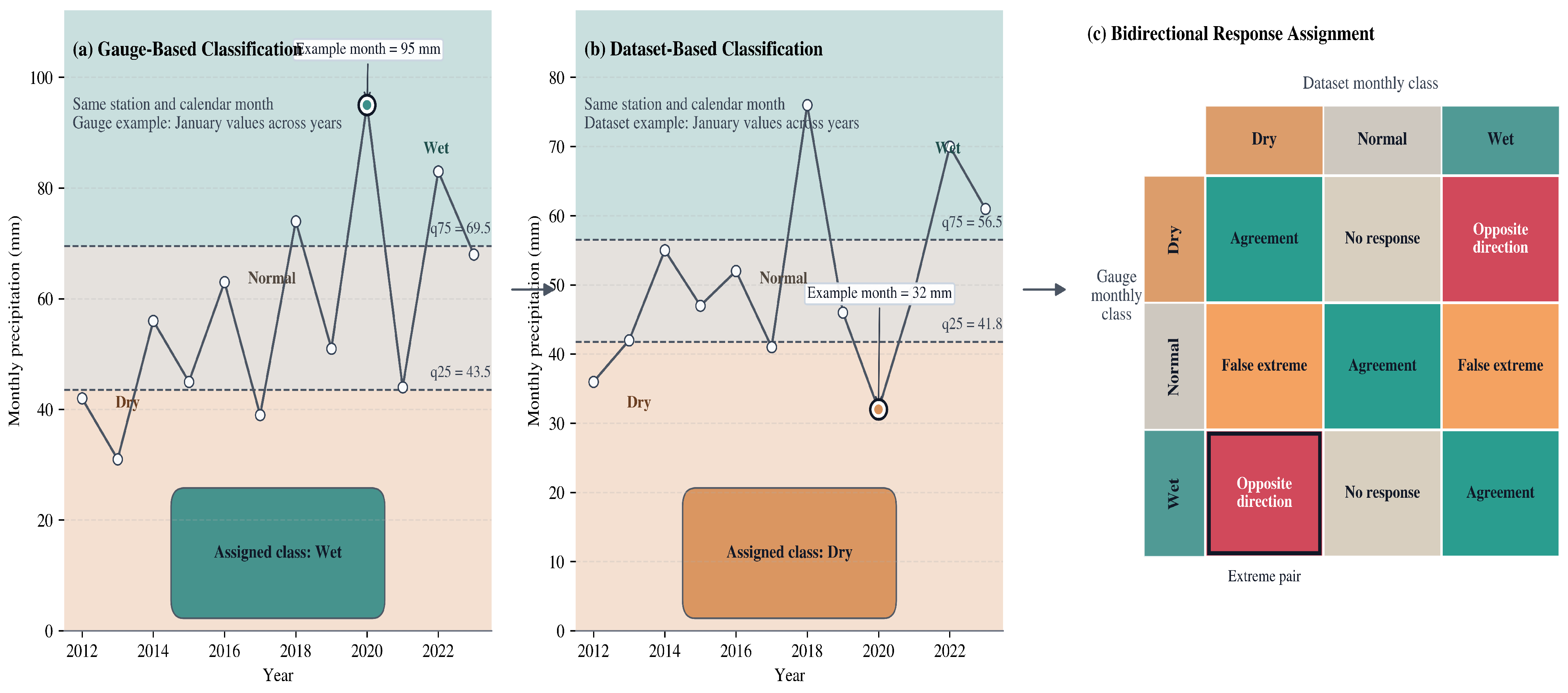
Figure 1. Schematic illustration of the bidirectional extreme-response analysis.
Sustainability 18 07982 g001
Figure 2. The gauge and gridded precipitation datasets (a) Temporal coverage (b) mean annual precipitation across the 11 basin stations within the common 1983–2011 comparison window.
Sustainability 18 07982 g002
Figure 3. UTRC: (a) location, (b) elevation distribution and river network, and (c) selected gauge locations and representative grid nodes used for the gridded precipitation datasets.
Sustainability 18 07982 g003
Figure 4. Cross-dataset boxplot summary for (a) the station-level R 2 , (b) R M S E and (c) BIAS distributions of each precipitation product.
Sustainability 18 07982 g004
Figure 5. Dataset-level frequencies of agreement, no-response, false-extreme, opposite-direction based on the BERA framework.
Sustainability 18 07982 g005
Figure 6. Wet, normal, and dry class hit rates of the gridded datasets based on the BERA framework. (within each product group, bars represent wet (1), normal (2), and dry (3) hit rates).
Sustainability 18 07982 g006
Figure 7. Station-by-dataset agreement structure in BERA: (a) overall agreement rate, (b) wet-class hit rate, (c) normal-class hit rate and (d) dry-class hit rate. Station labels on the horizontal axis include station elevations.
Sustainability 18 07982 g007
Figure 8. Elevation associations with station-aggregate BERA outcome rates: (a) agreement rate, (b) no-response rate, (c) false-extreme rate and (d) opposite-direction rate. Dashed lines show Theil–Sen trends, and the boxes report the Spearman rank statistics.
Sustainability 18 07982 g008
Figure 9. BERA agreement sensitivity to alternative percentile thresholds.
Sustainability 18 07982 g009
Table 1. Precipitation datasets used in this study.
DatasetDataset FamilySpatial ResolutionTemporal ResolutionData Availability
TSMS gauge observationsIn situ reference observationsPoint scaleMonthly totals1972–2011
CHIRPSSatellite-based, gauge-informed precipitation product 0.05 Monthly1981–present
GPCP v3.3Satellite–gauge merged global precipitation product 0.5 × 0.5 Monthly1983–present
ERA5Reanalysis-based precipitation product 0.25 Monthly1940–present
MSWEP v2.80Multi-source merged precipitation product 0.1 Monthly1979–present
CHELSAHigh-resolution, terrain-informed climatology-driven precipitation dataset∼30 arc-sec (∼1 km)Monthly1980–2018 *
CMIP6 EC-Earth3Climate-model-derived precipitation output 0.7 × 0.7 Monthly1980–2014
* Latest version used in this study.
Table 2. Number of gauge locations or grid cells within the basin for each dataset.
DatasetNumber of Gauge Locations or Grid Cells Within the BasinCount
TSMS GaugeIn situ gauge observations11
CHIRPS v3.0Satellite-based gridded precipitation product cells2244
GPCP v3.3Satellite–gauge merged grid cells19
CMIP6Climate model grid cells12
ERA5Reanalysis grid cells88
MSWEP v2.80Multi-source merged grid cells562
CHELSAHigh-resolution climatology grid cells80,601
Table 3. Station-level comparison between the ground observations and the precipitation products.
ProductMetricBaskale (2354 m)Batman (567 m)Bitlis
(1473 m)
Cizre
(377 m)
Diyarbakir (682 m)Ergani (1184 m)Hakkari (1649 m)Maden (1041 m)Siirt
(983 m)
Sivrice (1239 m)Yuksekova (1870 m)
CMIP6R20.0660.1580.1810.1790.1310.1700.1810.1970.1890.1200.126
Bias (mm)19.322.19−50.25−15.141.39−19.09−4.51−24.04−8.78−5.21−10.30
Mean (mm)56.7341.8253.8438.1140.1443.7757.4744.7148.5144.0555.97
Kendall’s τ 0.0240.0480.0360.0040.1010.1090.0040.1290.0080.149−0.016
CHIRPS v3.0R20.6480.6830.7380.7870.7300.7950.8040.7730.8160.1490.743
Bias (mm)−0.43−1.622.764.514.304.49−1.20−9.282.62−7.67−9.94
Mean (mm)36.9738.01106.8557.7543.0567.3660.7859.4759.9241.5956.33
Kendall’s τ −0.0810.0160.0040.032−0.077−0.0200.0480.081−0.028−0.028−0.012
GPCP v3.3R20.8140.9000.8970.9520.8780.9100.9790.8770.9370.1800.911
Bias (mm)9.4214.94−36.64−0.4513.87−8.35−3.95−14.212.462.28−16.99
Mean (mm)46.8254.5867.4552.7952.6254.5158.0454.5459.7551.5449.28
Kendall’s τ 0.056−0.060−0.117−0.032−0.024−0.0040.028−0.016−0.093−0.0160.028
ERA5R20.5490.8390.8290.8470.7800.8990.8020.8750.8340.1900.849
Bias (mm)5.8215.61−19.902.7518.02−3.4921.85−6.2511.2010.800.21
Mean (mm)43.2355.2484.1955.9956.7859.3883.8462.5068.5060.0666.48
Kendall’s τ −0.048−0.157−0.081−0.077−0.129−0.165−0.077−0.157−0.117−0.113−0.077
MSWEP v2.80R20.5140.6980.8410.8510.6580.7130.6760.6890.8820.1820.628
Bias (mm)3.7512.93−24.35−0.706.66−9.45−0.04−7.161.8210.17−8.90
Mean (mm)41.1552.5679.7452.5445.4153.4161.9461.5959.1159.4257.37
Kendall’s τ 0.129−0.198−0.129−0.077−0.254−0.306−0.238−0.315−0.133−0.315−0.177
CHELSAR20.9010.9930.9360.9850.9460.9450.9910.8680.9870.1650.961
Bias (mm)25.898.13−4.723.304.89−7.9015.88−19.2415.75−2.364.65
Mean (mm)63.3347.7399.3956.3543.5954.9077.7449.3673.0346.8670.88
Kendall’s τ −0.074−0.089−0.202−0.118−0.020−0.143−0.039−0.108−0.177−0.113−0.044
Disclaimer/Publisher’s Note: The statements, opinions and data contained in all publications are solely those of the individual author(s) and contributor(s) and not of MDPI and/or the editor(s). MDPI and/or the editor(s) disclaim responsibility for any injury to people or property resulting from any ideas, methods, instructions or products referred to in the content.