Integrated Energy, Time, and Cost Savings Assessment of Steel Billet Thermal Management: A Numerical Approach for Enhanced Industrial Sustainability

Abstract

Steel production involves energy-intensive thermal processes, where improvements in heat management can contribute to enhanced efficiency and reduced environmental impact. This study analyses the cooling and heating processes of steel billets in small-to-medium-sized steelworks, with the aim of identifying potential energy, time, and cost savings. Currently, billets leaving the casting process cool down freely in an open-air storage area from approximately their casting temperature to ambient conditions, and they are subsequently reheated to 1265 °C before rolling. A numerical model based on the finite difference alternating-direction implicit (ADI) method has been developed in MATLAB R 2025a to simulate these processes. The numerical implementation was verified against the analytical lumped-capacitance solution under the assumption of uniform billet temperature during slow cooling. For loading times of 15–30 min, the billets retained temperatures of 1112–806 °C after 15 days of insulated storage. Compared with reheating from 25 °C, the predicted heat savings were 672–936 MJ per billet, corresponding to fuel savings of 600–836 kWh_LHV, gross fuel-cost savings of EUR 18–25 per billet, and reheating-time reductions of 17.7–33.3 min. An improvement scenario was then analysed, consisting of placing 36 billets from each casting batch into an insulated container to reduce heat losses after casting. The results show that with reasonably well-insulated containers, billet temperatures can be maintained above 800 °C for up to 15 days. This increase in the inlet temperature to the reheating furnace reduces both the required energy and processing time. These results suggest that relatively simple thermal management strategies can improve energy efficiency and reduce operational demand in steel production, supporting more sustainable industrial processes.

1. Introduction

Global warming is one of the most important issues that humanity has to deal with. One of the main causes of global warming is greenhouse gases (GHGs) such as CO₂ or CH₄. In Europe, the main energy consumption sectors are as follows: 33.15% transport, 25.71% households, 24.99% industry and 13.54% services [1]. Reducing CO₂ emissions and final energy consumption are two of the main objectives of the European Union’s climate and energy policies. The EU has set the objective of further reducing greenhouse gas emissions by 80–95% by 2050, as described in Roadmap 2050 [2].

Energy-intensive sectors, like iron and steel industries, will be affected by CO₂ reduction measures [3]. Among the different industrial sectors, the steel industry is one of the major producers of carbon dioxide emissions in Europe [4]. The steel sector is a major industrial source of greenhouse gas emissions. Sarker et al. [5] examined the relationship between energy sources and carbon emissions in the South Asian iron and steel industry, whereas the International Energy Agency [6] provided a broader international inventory of CO₂ emissions from fuel combustion.

In this context, improving thermal management in existing industrial processes is a practical way to enhance sustainability without introducing major technological changes. In energy-intensive industries, reducing heat losses and making better use of residual heat can lead to significant improvements in energy efficiency and lower CO₂ emissions. Simple measures, such as improving insulation or maintaining higher temperatures between process stages, can reduce fuel consumption while keeping production conditions unchanged. For this reason, considering energy, time, and economic aspects together is important for developing more sustainable steel production processes, particularly in operations involving repeated heating and cooling stages such as billet production.

The steelmaking process is a complex process comprising several steps [7]. The process analysed in this research takes place in small–medium-sized steelworks where steel billets are produced and rolled. The billets leave the casting process at approximately 1500 °C and have dimensions of 0.145 m × 0.145 m × 8.4 m. These billets cool down freely in an open-air storage area from approximately 1500 °C to 25 °C (ambient temperature). First, the steel is in a liquid state, and solidification does not occur until the steel reaches temperatures of 1455 °C.

Depending on the clients’ demands and factory organization, the billets might be in the open-air storage area up to 30–40 days, so they usually have enough time to cool down until they are about 25 °C. Then, these cold billets are carried to the reheating furnace, and they are heated up until they reach 1265 °C. Then, they are rolled to their corresponding size. The reheating furnace is responsible for 40.85% of a steelworks’ natural gas consumption.

The understanding of heat removal phenomena during different processes is very important to steel industries. One of the processes in which they are more interested is the continuous casting process. The influence of the geometrical configuration and the operating conditions of the continuous casting machine must be known to guarantee safe operating conditions and good productivity and quality. Computational simulation has become a useful tool to simulate different industrial processes because it is a low-cost method that avoids physical experimentation. It also allows for the testing of critical operating conditions without any risk [8].

Early numerical descriptions of heat transfer during continuous casting were constrained by the computational resources available at the time. Choudhary et al. [9] developed a mathematical representation of heat transfer phenomena during continuous casting, while Choudhary and Mazumdar [10] subsequently provided a broader treatment of the associated transport phenomena. The general transport principles used in these early formulations were described by Geiger [11]. Improvements in numerical methods and computational capacity have since enabled more detailed transient and multidimensional models.

Previous numerical studies of steel billet cooling, solidification, and reheating have generally been based on the transient heat-conduction equation combined with convective and radiative boundary conditions. Santos et al. [12] developed a solidification heat transfer model for continuous-casting applications. Dubey and Srinivasan [13] analysed transient billet reheating while considering convection, radiation, and oxide-scale growth. Kakhki et al. [14] modelled continuous cooling to predict the microstructure and hardness of low-alloy steel. Kim [15] investigated transient slab heating in a direct-fired walking-beam furnace, whereas Han et al. [16] focused on the radiative heating characteristics of this type of furnace.

Different numerical methods have been used to solve these transient heat transfer problems. Santos et al. [12] used a finite difference formulation, whereas Dubey and Srinivasan [13] developed a finite-volume model for transient billet reheating. Kim [15] applied a control-volume approach to slab heating in a direct-fired walking-beam furnace, while Han et al. [16] focused on transient radiative heating in the same type of furnace. Dubey and Srinivasan [17] also used a control-volume formulation to investigate billet reheating and oxide-scale growth. These methods allow multidimensional billet temperature fields to be calculated during cooling and reheating.

Different approaches have also been used to represent steel solidification. Fixed-grid methods account for latent heat through a solid-fraction relationship [12,18], whereas single-domain methods incorporate the latent heat released at the solid–liquid interface [19]. Yu and Luo [20] represented phase-change behaviour using effective thermal conductivity and effective heat capacity. These studies provide the numerical basis for modelling billet temperature evolution. The governing equations, boundary conditions, and solidification treatment adopted in the present study are described in Section 2.

Although previous studies have proposed different numerical approaches for billet cooling, solidification, and reheating, they have mainly focused on continuous-casting control, furnace performance, heat transfer coefficients, or metallurgical quality. The use of passive insulated storage to preserve billet heat between casting and reheating has received less attention, particularly in small- and medium-sized steelworks where billets may remain in storage for several days.

Therefore, the objective of this study is to quantify the energy, reheating-time, and economic savings that may be achieved by storing hot billets in an insulated container instead of allowing them to cool freely in an open-air storage area. The actual billet free-cooling and reheating processes are first modelled. The model is subsequently applied to an improved scenario in which the 36 billets produced in each casting batch are placed in an insulated container. Different container loading times and storage periods are evaluated because the billet temperature at the reheating-furnace inlet depends on both parameters.

The main contribution of this study is the integrated numerical assessment of three consecutive stages: post-casting billet cooling, insulated intermediate storage, and furnace reheating. Unlike previous studies focused primarily on individual casting or reheating stages, the proposed approach relates the retained billet temperature to reheating energy demand, processing time, natural gas consumption, and operating cost. It also quantifies the influence of container loading time and storage duration, providing a preliminary decision-support tool for evaluating passive billet heat preservation in small- and medium-sized steelworks.

2. Methodology

2.1. Governing Equations and Heat Transfer Boundary Conditions

The transient temperature field in the steel billet is described by the three-dimensional heat-conduction equation. The nomenclature adopted in Equation (1) follows Çengel and Ghajar [21]:

$${\displaystyle \frac{\partial }{\partial x}}\left(k{\displaystyle \frac{\partial T}{\partial x}}\right)+{\displaystyle \frac{\partial }{\partial y}}\left(k{\displaystyle \frac{\partial T}{\partial y}}\right)+{\displaystyle \frac{\partial }{\partial z}}\left(k{\displaystyle \frac{\partial T}{\partial z}}\right)+{\dot{e}}_{gen}=\rho C{\displaystyle \frac{\partial T}{\partial t}} [\mathrm{W}/{\mathrm{m}}^3],$$

(1)

where T is the temperature field, k is the thermal conductivity, $\rho$ is the density, C is the specific heat, t is time and ${\dot{e}}_{gen}$ is the internal heat generation.

There are three main families of numerical methods: (1) finite differences, (2) finite elements and (3) finite volumes.

Numerous investigations start with Equation (1), but for correctly solving the billets heating problem within a furnace, it is crucial to precisely define the boundary conditions of the analysed process. With the total heat flux (${\dot{q}}_{tot}$) accounting for both convection and radiation heat flux [17], the following can be obtained:

$${\dot{q}}_{tot}=k{\displaystyle \frac{\partial T}{\partial n_n}}=h_{tot}\left(T_g-T_s\right) [\mathrm{W}/{\mathrm{m}}^2]$$

(2)

where n_n is the unit vector normal to the billet outer surface, T is the billet temperature field, k is the thermal conductivity of the billet, T_g is the furnace’s flue gas temperature and T_s is the billet surface temperature. The total heat transfer coefficient h_tot accounts for both the convective heat transfer coefficient h_conv and the radiative heat transfer coefficient h_r and is expressed as follows:

$$h_{tot}=h_{conv}+h_r=h_{conv}+\epsilon \sigma \left(T_g^2+T_s^2\right)\left(T_g-T_s\right) [\mathrm{W}/{\mathrm{m}}^2·\mathrm{K}]$$

(3)

where ε is the emissivity of the billet surface and σ is the Stefan–Boltzmann constant.

In ref. [13], although they start from the same equation, the boundary conditions are different and also consider the billet direct heat exchange with the inner surface of the furnace. This time, the heated billets also consider convection and radiation heat exchange with the gas, but the equation is represented as follows:

$$\begin{gathered} {\dot{q}}_{tot}=k{\displaystyle \frac{\partial T}{\partial n_n}}={\displaystyle \frac{\sigma {\epsilon }_s}{\left[1-\left(1-{\epsilon }_s\right)\left(1-A_{gs}\right)\right]}}\left({\epsilon }_g{T}_g^4-A_{gs}{T}_s^4\right)+h_{conv}\left(T_g-T_s\right) \\ +\sigma {\epsilon }_{sw}\left(T_w^4-T_s^4\right) [\mathrm{W}/{\mathrm{m}}^2] \end{gathered}$$

(4)

where T_g is the furnace gas temperature, T_s is the billet surface temperature, T_w is the furnace internal wall temperature, ε_g is flue gas emissivity, A_gs is the absorptivity of the furnace flue gas and ε_sw is the direct exchange factor between the furnace inner wall and the billet surface.

Starting from Equation (1), M. E. Kakhki et al. [14] propose applying different boundary conditions to analyse the billet cooling process. The heat is transferred by convection and radiation during the cooling, and the boundary condition is written as follows:

$${\dot{q}}_{tot}=-k{\displaystyle \frac{\partial T}{\partial n_n}}=h_{conv}\left(T_s-T_a\right)+\epsilon \sigma \left(T_s^4-T_a^4\right) [\mathrm{W}/{\mathrm{m}}^2]$$

(5)

where h_conv is the convective heat transfer coefficient, ε is the billet surface emissivity, σ is the Stefan–Boltzmann constant, T_s is the billet surface temperature and T_a is the ambient temperature.

The solidification of the steel is a complex phase to simulate using numerical methods.

$$k_{eff}=f_s{·k}_s+m\left(1-f_s\right)·k_l [\mathrm{W}/\mathrm{m}·\mathrm{K}]$$

(6)

$$C_{eff}=C-L\left({\displaystyle \frac{\partial f_s}{\partial T}}\right) [\mathrm{J}/\mathrm{k}\mathrm{g}·\mathrm{K}]$$

(7)

Here, k_l and k_s are the liquid and solid thermal conductivity coefficients, respectively, m is a parameter [22], f_s is the solid fraction, C is the latent heat of fusion [J/kg], and $L\left({\displaystyle \frac{\partial f_s}{\partial T}}\right)$ is the pseudo-specific heat.

The differential equation to predict the temperature field in a solid is a linear differential equation of partial second-order derivatives [23]. If the thermal conductivity of the steel ($k_{steel}$) is considered independent of the temperature and reordering Equation (1), the Equation (8) differential equation is obtained:

$${\displaystyle \frac{k_{steel}}{\rho ·C_s}}·\left({\displaystyle \frac{{\partial }^{2}T}{{\partial x}^2}}+{\displaystyle \frac{{\partial }^{2}T}{{\partial y}^2}}+{\displaystyle \frac{{\partial }^{2}T}{{\partial z}^2}}\right)+{\displaystyle \frac{{\dot{e}}_{gen}}{\rho ·C_s}}={\displaystyle \frac{\partial T}{\partial t}} [\mathrm{K}/\mathrm{s}]$$

(8)

where $k_{steel}$ is the steel thermal conductivity $\left[\mathrm{W}/\mathrm{m}·\mathrm{K}\right]$, $\rho$ is the steel density $\left[\mathrm{k}\mathrm{g}/{\mathrm{m}}^3\right]$, $C_s$ is the steel specific heat $\left[\mathrm{J}/\mathrm{k}\mathrm{g}·\mathrm{K}\right]$, ${\dot{e}}_{gen}$ is the term associated to the internal heat generation $\left[\mathrm{W}/{\mathrm{m}}^3\right]$, $T$ is temperature field $\left[\mathrm{K}\right]$ and $t$ is time [s].

To solve any transient problem of heat transfer by conduction, the temperature field in the solid $T(x,y,z,t)$ must be known. The temperature distribution is obtained by integrating this differential equation considering the correct initial and boundary conditions. In this work, the solution to the temperature field is obtained by numerical methods, specifically the alternating-direction implicit finite difference method.

2.2. Alternating-Direction Implicit Method

Since the billet length (8.4 m) is two orders of magnitude higher than the billet sides (0.145 m × 0.145 m), heat transfer in the longitudinal direction can be neglected, except near the billet ends. Therefore, the cooling and reheating processes are modelled as a two-dimensional transient heat-conduction problem in the billet cross-section.

The differential equation for a transient two-dimensional problem without internal heat generation is given by Equation (9).

$${\displaystyle \frac{k_{steel}}{\rho ·C_s}}·\left({\displaystyle \frac{{\partial }^{2}T}{{\partial x}^2}}+{\displaystyle \frac{{\partial }^{2}T}{{\partial y}^2}}\right)={\displaystyle \frac{\partial T}{\partial t}} [\mathrm{K}/\mathrm{s}]$$

(9)

Figure 1 shows the variation in the thermal conductivity and the specific heat of the steel in function of the temperature. Since these properties affect thermal diffusivity, temperature gradients, and transient cooling and heating rates, representative average values corresponding to the temperature interval between the initial billet temperature and ambient temperature were used in the simulations. This simplification preserves a linear ADI formulation and enables consistent comparison among the investigated scenarios. Consequently, the absolute temperature histories and processing times should be regarded as engineering estimates. A temperature-dependent implementation would require updating the local properties at every node and time step using reliable grade-specific data and is proposed for future work.

$$\begin{gathered} {\displaystyle \frac{k_{steel}}{\rho ·C_s}}·\left({\displaystyle \frac{T_{i-1,j,n}^{*}-2·T_{i,j,n}^{*}+T_{i+1,j,n}^{*}}{{∆x}^2}}+{\displaystyle \frac{T_{i,j-1,n}-2·T_{i,j,n}+T_{i,j+1,n}}{{∆y}^2}}\right) \\ ={\displaystyle \frac{T_{i,j,n}^{*}-T_{i,j,n}}{∆t/2}} [K/\mathrm{s}] \end{gathered}$$

(10)

The numerical method used to solve this two-dimensional transient equation is the alternating-direction implicit method. The method consists in applying two finite difference equations alternatively in two different steps. Each step describes a $∆t$/2 magnitude of time. The first step is only implicit in the x direction, and the second step is implicit in the $y$ direction [23].

Therefore, at time $n$, the temperature distribution is $T_{i,j,n}$, and the equation is applied in the $x$ direction with a $∆t$/2 increment in time. The result is the temperature distribution in $n+∆t/2$, which is called $T_{i,j,n}^{*}$. Thus, Equation (9) can be written in a finite difference form as in Equation (10).

Considering that $∆x=∆y$ and therefore $\tau ={\displaystyle \frac{∆t}{∆x^2}}·{\displaystyle \frac{k_{steel}}{\rho ·C_s}}={\displaystyle \frac{∆t}{∆y^2}}·{\displaystyle \frac{k_{steel}}{\rho ·C_s}}$, Equation (10) can be rearranged, and as a result, an implicit equation for a single node in the first step of the integration is obtained. The unknown terms are on the left and the known terms on the right:

$${-T}_{i-1,j,n}^{*}+2·\left({\displaystyle \frac{1}{\tau }}+1\right)·T_{i,j,n}^{*}-T_{i+1,j,n}^{*}=T_{i,j-1,n}+2·\left({\displaystyle \frac{1}{\tau }}-1\right)·T_{i,j,n}+T_{i,j+1,n} [\mathrm{K}]$$

(11)

After performing the first step integration, $T_{i,j,n}^{*}$ temperature distribution is calculated. Then, starting from the $T_{i,j,n}^{*}$ temperature distribution in the moment $n+∆t/2$, the finite difference equation is applied in the $y$ direction with a $∆t/2$ increment in time. This time, the result is the temperature distribution in $n+1$, which is called $T_{i,j,n+1}$. Then, Equation (9) can be written in finite difference form as in Equation (12).

$$\begin{array}{c}\hspace{1em} {\displaystyle \frac{k_{steel}}{\rho ·C_s}}·\left({\displaystyle \frac{T_{i-1,j,n}^{*}-2·T_{i,j,n}^{*}+T_{i+1,j,n}^{*}}{{∆x}^2}}+{\displaystyle \frac{T_{i,j-1,n+1}-2·T_{i,j,n+1}+T_{i,j+1,n+1}}{{∆y}^2}}\right)\hfill \\ ={\displaystyle \frac{T_{i,j,n+1}{-T}_{i,j,n}^{*}}{∆t/2}} [\mathrm{K}/\mathrm{s}]\hfill \end{array}$$

(12)

Rearranging Equation (12), the implicit equation for a single node in the second step of the integration is obtained, for the $n+1$ moment. The unknown terms are on the left and the known terms on the right.

$$T_{i,j-1,n+1}+2·\left({\displaystyle \frac{1}{\tau }}+1\right)·T_{i,j,n+1}+T_{i,j+1,n+1}=T_{i-1,j,n}^{*}+2·\left({\displaystyle \frac{1}{\tau }}-1\right)·T_{i,j,n}^{*}-T_{i+1,j,n}^{*} [\mathrm{K}]$$

(13)

In each $∆t$ interval of time, the boundary conditions in $x$ are updated in the first step and in $y$ in the second step. The MATLAB R2025a code developed to solve these equation systems for the actual cooling process of the billets is shown in Appendix A. Note that this code considers the solidification process if the initial temperature of the cooling process starts over the solidification temperature. The code for the actual heating process and for any of the proposed improved heating processes is similar to the Appendix A code. However, it is simpler since the reheating furnace does not reach the melting temperature. The required changes in the code are the next ones: ambient temperature should be that of the furnace flue gas, initial temperature should be the billet inlet temperature to the reheating furnace, and the formulas to obtain the convection coefficients are different since the billet surfaces are heated instead of cooled.

A uniform mesh with 14 divisions in each cross-sectional direction and a time step of 1 s was applied consistently to all simulations. Although a formal mesh- and time-step-independence analysis was not conducted, the numerical implementation was verified against the analytical lumped-capacitance solution.

Figure 2 summarises the computational procedure. The model first defines the input parameters and initializes the temperature field. It then applies the boundary conditions and performs the two ADI half-steps. The calculation is repeated until the stopping criterion for cooling, insulated storage, or reheating is satisfied. Finally, the temperature fields, heat losses, reheating time, fuel consumption, and gross fuel-cost savings are calculated. The complete MATLAB implementation is provided in Appendix A to facilitate reproducibility.

2.3. Solidification

When the billets get out of the electric arc furnace, they have a temperature of about $1500 °\mathrm{C}$. Knowing that the solidification temperature of the steel is $1455 °\mathrm{C}$, when the billets get out of the casting, they are in a liquid state. Thus, this solidification process is included in the code of Appendix A.

In this work, to simulate the solidification, an equivalent value for the specific heat ($C_{s\_eq}$) is proposed, which is a similar approach to the one used in [20]. This equivalent specific heat is calculated as in Equation (14), and it is associated with all the nodes that are over the solidification temperature. Thus, the solidification latent heat is distributed among the 45 °C required for cooling from the initial temperature to the solidification temperature. Then, once the nodes’ temperatures are below the solidification temperature, the specific heat of the solid steel is used in the calculations. Even if this assumption could introduce slight errors, the whole billet solidification process occurs in about 15 min. This is a very short time within the 3- to 15-day simulation periods considered in this research. Furthermore, since the latent heat of solidification is distributed along the 45 °C (difference between 1500 °C and 1455 °C) of the liquid phase cooling, the nodes that are over the solidification temperature will have a slightly higher temperature than in reality. Thus, since the temperature gradient between internal liquid nodes and surface solid nodes will be higher than the real one, this assumption will estimate slightly faster cooling of the billet while there are still liquid fractions within the billet. Once the solidification is complete, this assumption will generate no error. Then, the energy, time and economic calculations will be done from a security point of view.

$$C_{s\_eq}={\displaystyle \frac{q_{liq}+q_{sol}}{T_i-T_{sol}}} [\mathrm{J}/\mathrm{k}\mathrm{g}·\mathrm{K}]$$

(14)

Here, $T_i$ is the initial temperature of the steel billet, $T_{sol}$ is the solidification temperature of the steel, $q_{sol}$ is the latent heat of the solidification with a value of 290 $\mathrm{k}\mathrm{J}/\mathrm{k}\mathrm{g}$ [24], and $q_{liq}$ is the heat transfer between the initial temperature and the solidification temperature, which can be expressed as follows:

$$q_{liq}=C_{sl}·\left(T_i-T_{sol}\right) [\mathrm{J}/\mathrm{k}\mathrm{g}]$$

(15)

where $C_{sl}$ is the average specific heat between $T_i$ and $T_{sol.}$

Therefore, the Appendix A code calculates and uses this equivalent specific heat $\left(C_{s\_eq}\right)$ when there are nodes above the solidification temperature. The Appendix A code uses the solid steel specific heat $(C_s$) when the node temperature is below the solidification temperature.

2.4. Initial and Boundary Conditions

The initial temperature of the steel billet, $T_i$, is assumed to be uniform in the entire body for all the analysed cases:

$${\left.T\right|}_{t=0}=T_i [\mathrm{K}]$$

(16)

For the boundary conditions of both cooling and heating processes, the approach used in [14] is considered. The heat can be removed or added from the billet’s surface by convection and radiation. Thus, the boundary conditions can be described as follows:

$${\dot{q}}_{conv}=h_{conv}·\left(T_s-T_a\right) [\mathrm{W}/{\mathrm{m}}^2]$$

(17)

$${\dot{q}}_{rad}=\epsilon ·\sigma ·\left(T_s^4-T_a^4\right) [\mathrm{W}/{\mathrm{m}}^2]$$

(18)

where ${\dot{q}}_{conv}$ is the heat transfer by convection $[\mathrm{W}/{\mathrm{m}}^2]$, $h_{conv}$ is the convective heat transfer coefficient $[\mathrm{W}/{\mathrm{m}}^2·\mathrm{K}]$, ${\dot{q}}_{rad}$ is the heat flux by radiation [W/m²], $\epsilon$ is the emissivity of the billet surface, σ is the Stefan–Boltzmann constant, $T_s$ is the surface temperature and $T_a$ is the ambient temperature (for the heating case, the ambient temperature will be the furnace flue gas temperature).

The term $h_{conv}$ is different depending on the orientation of the face. However, it is then considered constant for each billet face along the whole cooling or heating process because of slight variations in this coefficient due to the billet surface to air temperature variation barely affecting the simulation results. On the other hand, due to its importance, a parametric analysis is done to see the influence of the considered billet surface emissivity in the simulation results.

2.5. Lumped-Capacitance Analysis for Numerical Verification

Some bodies behave like “lumps”, as if their temperature was always uniform during a cooling or heating process. The temperature in those bodies is only a function of time, $T\left(t\right).$ Heat transfer analysis that uses this idealization is called lumped system analysis. This method will help to validate the Appendix A MATLAB code.

Consider a billet of mass $m$, volume $V_{billet}$, total surface area $A_{billet}$, density $\rho$, specific heat $C_s$ and initial temperature $T_i$. At time $t=0$, the body is left in a place where the ambient temperature is $T_a$ and the heat transfer between the body and the ambient starts. The total heat transfer coefficient $h_{tot}$ of this hypothetical process will be small enough so as to provide an extremely low Biot number. Therefore, the conduction heat flow movement within the billet will be much faster than the heat transfer from the billet surface to the ambient. Then, the billet temperature will be homogeneous during the whole heat transfer process. The analysis works for both $T_i>T_a$ and $T_i<T_a$.

For a differential time interval $dt$, the body’s temperature increases by a differential amount $dT$ (if $T_i<T_a)$. The energy balance of the billet for the time interval $dt$ is the following:

$$h_{tot}·A_{billet}·\left(T_a-T\right)·dt=m·C_s·dT [\mathrm{J}]$$

(19)

where m is the billet mass (m = $\rho ·\mathrm{V}$), d(T − T_a) is the differential temperature difference between the billet and the surroundings, and Ta is assumed constant. So, Equation (19) can be rearranged as follows:

$${\displaystyle \frac{d(T-T_a)}{T-T_a}}={\displaystyle \frac{h_{tot}·A_{billet}}{\rho ·V_{billet}·C_s}}·dt [-]$$

(20)

If the equation is integrated from $t=0$, at which $T=T_i$, to any time $t$, at which $T=T\left(t\right)$:

$$ln{\displaystyle \frac{T\left(t\right)-T_a}{T_i-T_a}}=-{\displaystyle \frac{h_{tot}·A_{billet}}{\rho ·V_{billet}·C_s}}·t [-]$$

(21)

Taking the exponential of both sides of the equation, the result is the following:

$${\displaystyle \frac{T\left(t\right)-T_a}{T_i-T_a}}=e^{-bt} [-]$$

(22)

where $b$ is a positive quantity whose dimension is $[1/\mathrm{s}]$:

$$b={\displaystyle \frac{h_{tot}·A_{billet}}{\rho ·V_{billet}·C_s}} [1/\mathrm{s}]$$

(23)

The lumped analysis system is valid if the Biot number is $Bi\le 0.1$ [21]. The Biot number is calculated using Equation (25). $L_C$ is the characteristic length of the billet, and $k$ is the conduction coefficient of the steel.

$$L_C={\displaystyle \frac{V_{billet}}{A_{billet}}} [\mathrm{m}]$$

(24)

$$Bi={\displaystyle \frac{h_{tot}·L_C}{k}} [-]$$

(25)

The smaller the Biot number, the more precise the lumped system analysis is. Considering very small Biot numbers leads to extremely long cooling periods. Considering the available computer simulation capacity, the smallest Biot number that has been reasonable to simulate is $Bi=0.0001$. Then, from Equation (25), the total heat transfer coefficient can be obtained, referred to as $h_{validation}$. This coefficient is used in the lumped system analysis and in the code of Appendix A in order to analyse the change in temperature over time. Using this extremely low $h_{validation}$ in the Appendix A code leads to a temperature distribution in the billet that is only a function of time $T(x,y,t)\approx T\left(t\right).$ Note that, when using the Appendix A code, the equations of the boundary conditions have to be modified since both the radiation and convection effects are now considered within $h_{validation}$. The radiation equation of the boundary conditions of the Appendix A code has to be cancelled out, and in the convection equation, $h_{validation}$ must be used instead of $h_{conv}$, since $h_{validation}$ is equal for all the billet faces.

Root-mean-square error (RMSE) has been used as a measure of the deviation of the simulation result (${\widehat{z}}_i={\widehat{T}}_{centre\_i}$) against the lumped system analysis result ($z_i=T_i$) [25]. The RMSE for the whole cooling process has been calculated, with n being the number of data points of the whole cooling process:

$$RMSE=\sqrt{{\displaystyle \sum _{i=1}^n}{\displaystyle \frac{{\left({\widehat{z}}_i-z_i\right)}^2}{n}}}$$

(26)

where z_i represents the numerical simulation temperature and ${\widehat{z}}_i$ represents the lumped-capacitance solution temperature.

2.6. Energy Efficiency Improvement Method

Once the Appendix A simulation code for the actual cooling process has been validated through the comparison to the lumped system analysis, the code can be used to reliably simulate the actual free cooling of the billets in ambient air (this is the code presented in Appendix A). To simulate the actual heating within the reheating furnace from the ambient temperature to the reheating-furnace exit temperature, it is required to make the abovementioned small modifications to the Appendix A code. Thus, the actual case cooling and heating parameters are first presented, and then the proposed passive energy efficiency measures are detailed.

2.6.1. Actual Case

The billets, once that they are out of the casting process, are left in ambient air. There, they cool down to ambient temperature. This means that they go from $1500 °\mathrm{C}$, which is the exit temperature from the casting process, to ambient temperature ($25 °\mathrm{C}$). Subsequently, the billets are put in the reheating furnace, and they are heated up from ambient temperature ($25 °\mathrm{C}$) to $1265 °\mathrm{C}$.

In the analysed steelworks, the billets are inside the reheating furnace for 3 h. During those 3 h, the billets reach a homogenous temperature before lamination. The reheating furnace is divided into three parts where the ambient temperatures are usually about: $1250 °\mathrm{C}$, $1280 °\mathrm{C}$ and $1270 °\mathrm{C}$. The simulation of the heating process was made using the average temperature of the three parts, $1265 °\mathrm{C}$.

2.6.2. Energy Efficiency Improved Case

In this case, instead of storing the billets in ambient air, the storage takes place within an insulated container. The improvement method has the purpose of avoiding the heat loss the billets suffer when they cool down freely in the outdoor storage area of the factory. By storing the billets in containers that act like insulators, the heat loss rate should be drastically reduced.

Once the billets get out of the casting process, they should be placed in the containers as fast as possible. The new cooling process will have two parts. The first part of this new cooling process is similar to the actual one, and it considers the time it takes to store all the billets of a cast into the container. For this research, this first period will be considered to be between 5 and 30 min. In this first period, the cooling process will be very fast. Then, when the container is closed, the billet cooling velocity will drastically slow down. Then, the billets pack will behave as a lumped system, where the billets’ temperature mainly depends on time. Thus, the heat loss of the billets will be partially avoided by keeping the billets hot until the billets are carried to the next process (the heating process). The new heating process will be faster and more efficient, since the billets will be introduced in the reheating furnace at a much higher temperature.

In the studied case, each cast produces a 6 × 6 pack of billets, and considering the billets’ dimensions, the packs’ dimensions are 0.87 m × 0.87 m × 8.4 m. In order to avoid problems when the billets are placed in the containers, the container’s inner dimensions should be bigger than those of the pack. For this research, inner dimensions of 1 m × 1 m × 8.5 m. are considered, as shown in Figure 3.

The average thermal conductivity of the insulation layer of the container walls is considered to be 0.037 [W/m∙K], and the calculus is done assuming an insulation layer thickness of 0.6 m. No thermal bridges are considered. Furthermore, since the insulation layer thermal resistance is orders of magnitude bigger than the inner and outer surface thermal resistances and the container’s metal structure layer thermal resistances, only the insulation layer thermal resistance is considered in the calculations. Then, the one-dimensional steady state heat transfer through the walls of the containers can be expressed as follows:

$${\dot{Q}}_{container}={\displaystyle \frac{T_{in}-T_{out}}{\frac{e}{k_{wall}}}} ·A_c [\mathrm{W}]$$

(27)

where ${\dot{Q}}_{container}$ is the heat transfer rate through the container [W], T_out and T_in are the outside and inside temperatures of the container [K], e is the thickness of the container walls [m], k_wall is the considered average conductivity of the insulation layer [W/m∙K], and A_c is the internal surface area of the container [m²].

Knowing that inside a container there are 36 billets, the heat loss rate associated with each billet can be obtained as follows:

$${\dot{Q}}_{billet}={\displaystyle \frac{{\dot{Q}}_{container}}{36}} [\mathrm{W}]$$

(28)

The container heat loss is calculated for the complete 36-billet batch and then allocated equally among the billets using Equation (28). Thus, the model does not treat the billets as 36 independently exposed bodies. The per-billet formulation assumes that the billet pack reaches an approximately uniform temperature and that the total container heat loss can be distributed according to the billet mass. Under these assumptions, the total energy and gross fuel-cost savings scale linearly with the number of processed billets.

The thermal mass of the air inside the container is negligible compared with that of the billet pack. Internal convection and radiation are assumed to produce a relatively uniform internal temperature after the initial transient temperature following container closure. Therefore, the billet surface, internal air, and inner-wall temperatures are approximated as equal. This approximation is expected to be less accurate during the initial period following container closure. Once the internal temperature becomes approximately uniform, the average heat-loss rate allocated to each billet can be expressed as follows:

$${\dot{Q}}_{billet}={h_{eq}·A_{billet}·\left(T_s-T_{out}\right)\approx h}_{eq}·A_{billet}·\left(T_{in}-T_{out}\right) [\mathrm{W}]$$

(29)

where h_eq is the equivalent billet surface to the outer air total heat transfer coefficient [W/m²∙K], A_billet is the billet surface area [m²], and T_s is the billet surface temperature [K].

If Equations (28) and (29) are equated, h_eq can be obtained. As demonstrated by Equation (30), h_eq is the equivalent heat transfer coefficient that the billets have inside the container for (T_s − T_out) ≈ (T_in − T_out):

$${\displaystyle \frac{\frac{T_{in}-T_{out}}{\frac{e}{k_{wall}}} ·A_c}{36}}=h_{eq}·A_{billet}·\left(T_{in}-T_{out}\right) \to h_{eq}={\displaystyle \frac{A_c/A_{billet}}{36\left(\frac{e}{k_{wall}}\right)}}$$

(30)

Using this new equivalent coefficient, the boundary conditions of the billet cooling process change, because the heat transfer coefficient is different. With these new conditions, the cooling of the billets should be slower. This simulation made with the new h_eq shows the cooling process inside the containers. As for the verification case, the equations of the boundary conditions have to be modified since both the radiation and convection effects are now considered within h_eq. In Appendix A, the radiation equation of the boundary conditions has to be cancelled out, and in the convection equation h_eq must be used instead of h_conv, since h_eq is equal for all the billet faces.

As mentioned before, using the containers, the inlet temperature of the billets in the reheating furnace will be higher; therefore, there are time, energy and money savings in the reheating furnace. By knowing the actual time needed to heat up each billet form from 25 °C to 1265 °C and the necessary heat for that, the energy and time savings can be obtained for the new heating process.

A reheating-furnace efficiency of 31.10% was assumed for the case study and applied consistently to all scenarios. It is defined as the ratio between the heat absorbed by the billet and the natural gas energy supplied on an LHV basis. The lower heating value of natural gas was set to 10.45 kWh_LHV Nm⁻³ (37,620 kJ/Nm³), with a cost of EUR 0.03 kWh_LHV. Since detailed plant data were not available to determine variations in furnace efficiency, it was assumed to remain constant. Therefore, the reported monetary values represent estimated gross fuel-cost savings under the assumed operating conditions. Container investment, handling, operation, and maintenance costs were not considered because plant-specific cost data were unavailable.

The main modelling assumptions are two-dimensional heat conduction, a uniform initial billet temperature, representative temperature-independent thermophysical properties, constant ambient and furnace temperatures, prescribed surface emissivity, negligible longitudinal heat transfer except near the billet ends, homogeneous container insulation, negligible thermal bridges, and constant furnace efficiency. These assumptions reduce computational complexity and allow consistent comparison among the investigated scenarios.

3. Results and Discussion

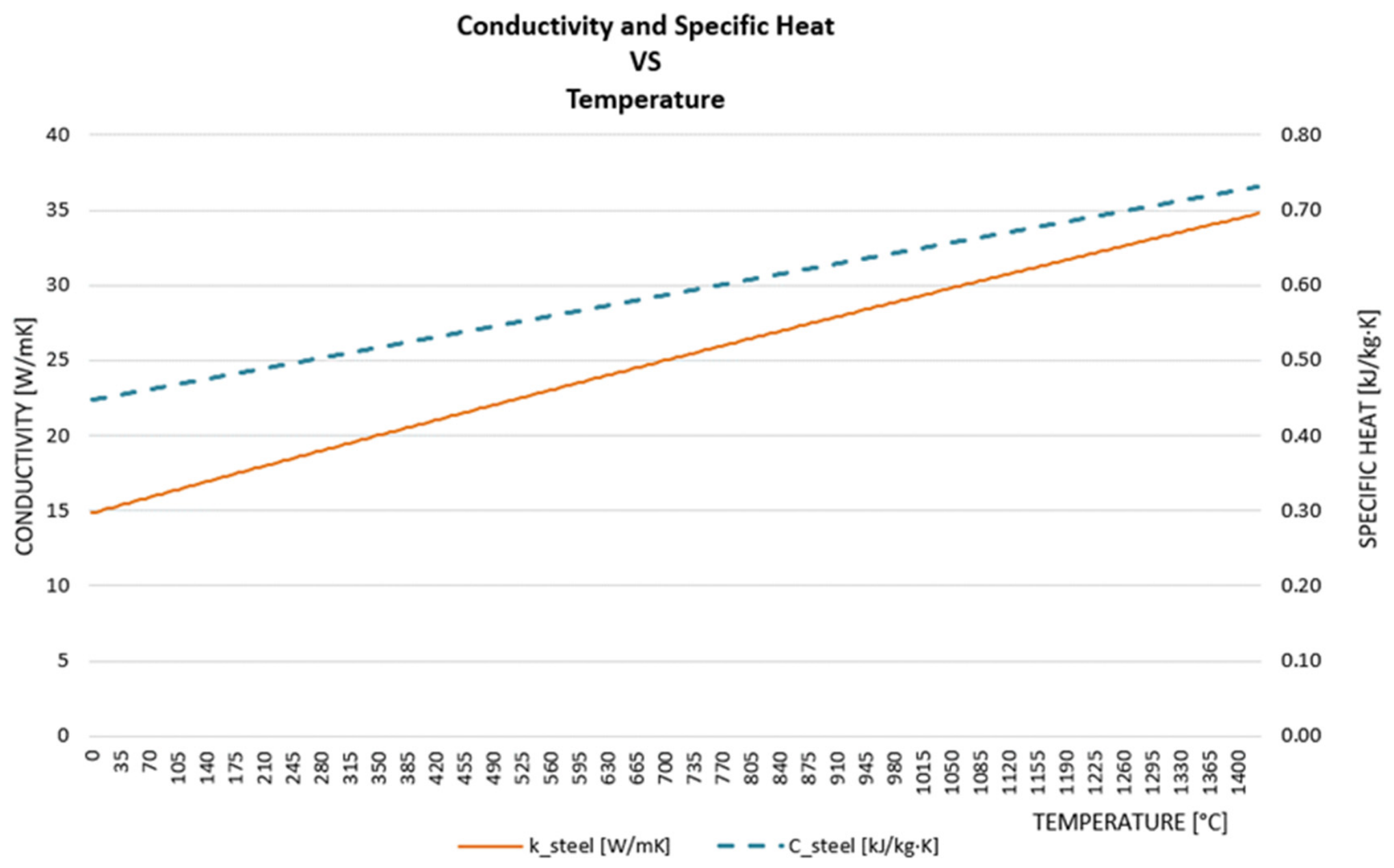
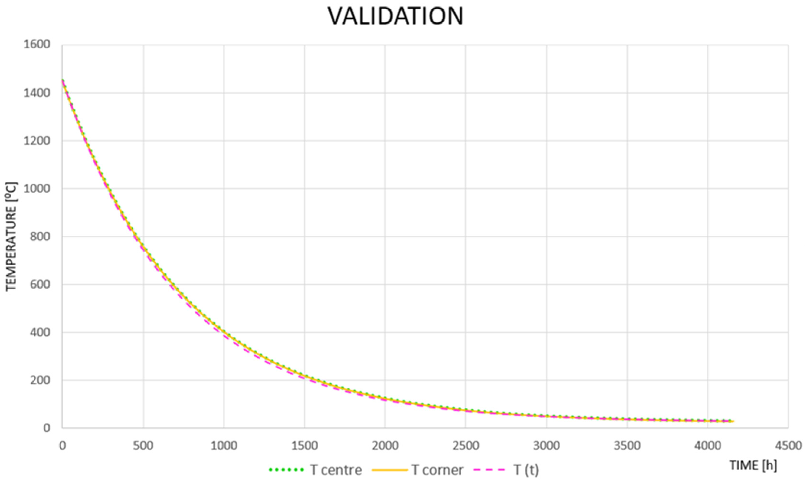
3.1. Numerical Verification

Starting from h_validation = 0.07 [W/m²∙K], which makes a Biot number of 0.0001, the code of Appendix A is validated. In Figure 4, the billet temperature variation in function of time is shown. Using the simulation code, it can be seen that the billet temperature field is homogenous from 1450 °C to 25 °C (ambient temperature). The three temperatures shown in the graphic are: temperature of the centre of the billet (T_centre), the temperature of one of the corners of the billet (T_corner), and the temperature obtained from the lumped system analysis equation (T(t)) (Equation (22)).

As illustrated in Figure 4, the lumped-capacitance solution predicts slightly faster cooling than the numerical model. After 173 days, the lumped-capacitance solution predicted a billet temperature of 29.76 °C, whereas the numerical model predicted centre and corner temperatures of 30.79 °C and 30.78 °C, respectively. The RMSE of 10.43 °C corresponds to approximately 0.73% of the 1425 °C verification interval. The final difference between the lumped-capacitance solution and the numerical centre temperature was 1.03 °C. This agreement verifies the numerical implementation under the limiting condition of Bi = 0.0001.

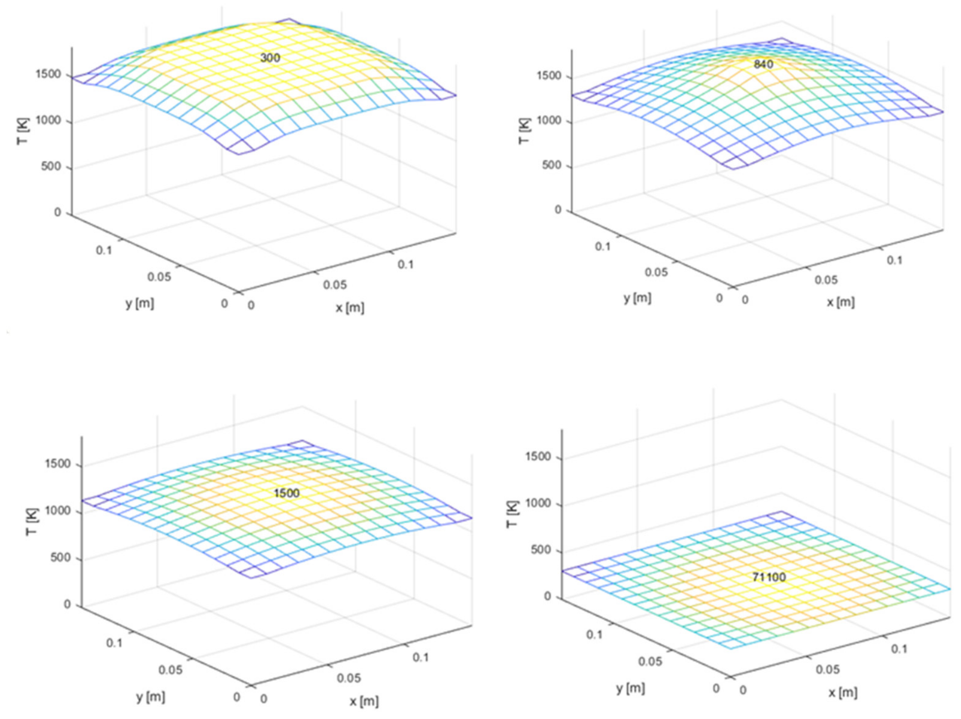
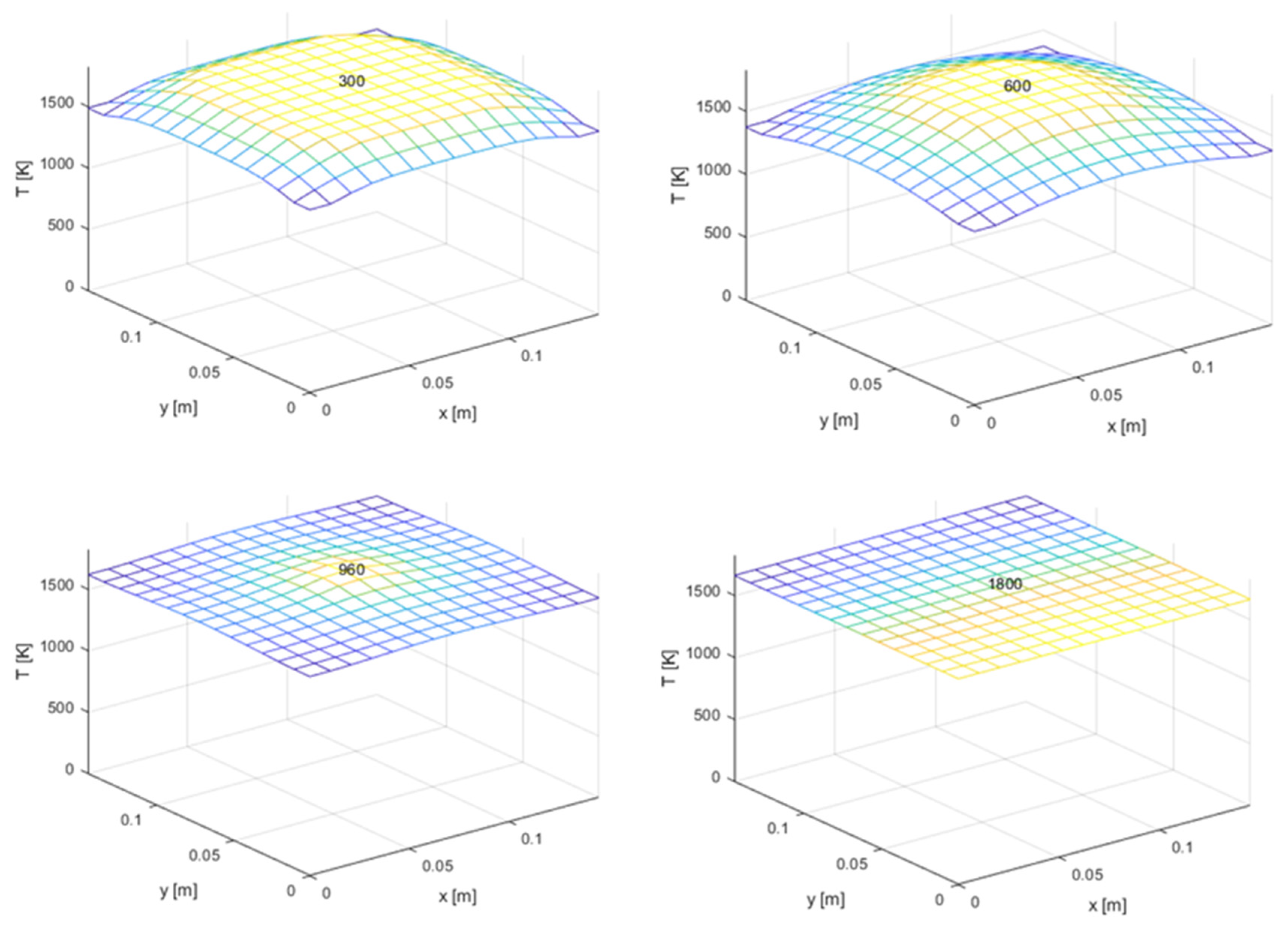
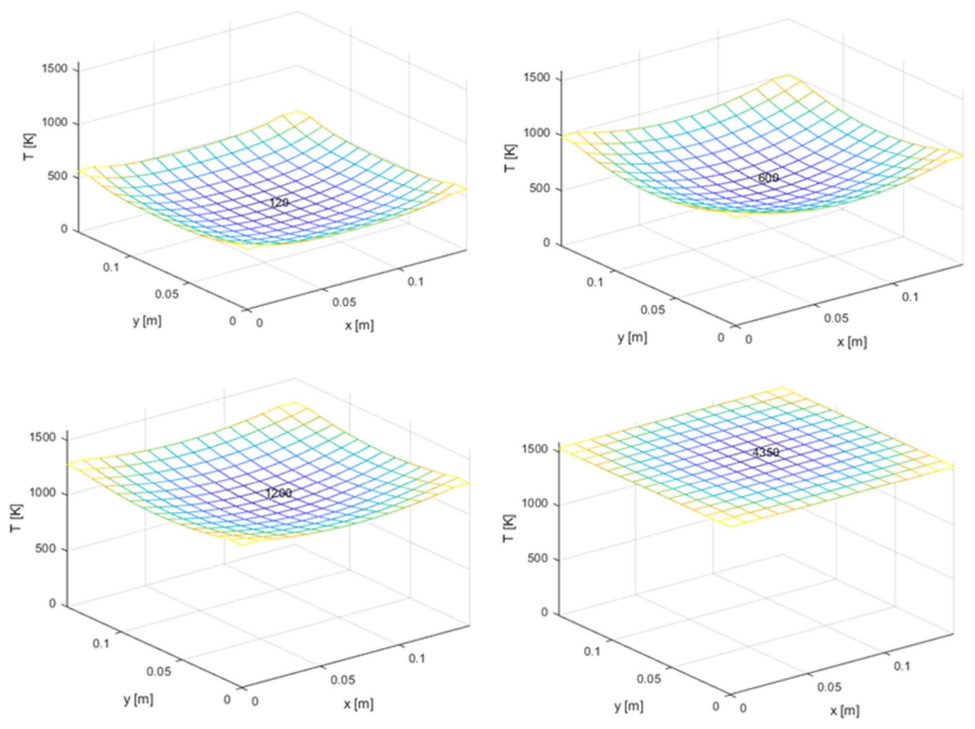
3.1.1. Actual Case Results

Using the code from Appendix A, the results of the actual cooling process are obtained (Figure 5 and Figure 6). The code follows what is described in Section 2.2 and the initial and boundary conditions explained in Section 2.4. First, a parametric study regarding the billet surface emissivity is presented. The parametric study results for cooling from 1500 °C to 25 °C are represented in Figure 5, whereas the reheating results from 25 °C to 1265 °C are represented in Figure 6. The values of the specific heat and thermal conductivity of the solid steel are considered to be C_s = 0.64 [kJ/kg∙K] and k_steel = 25.2 [W/m∙K].

During cooling, the time is stopped when the highest temperature on the billet is lower than 30 °C. During heating, the time is stopped when the lowest temperature in the billet is higher than 1260 °C. The heat transfer for a billet during cooling is 1.66 GJ and during heating is 1.064 GJ.

The parametric study with different values for emissivity revealed that when the considered emissivity values are higher, the estimated time for the cooling process is considerably decreased. The relationship between the considered emissivity and the needed time in the heating process follows the same pattern; when the considered emissivity values are higher, the estimated time is considerably lower.

For the first 15 min of the actual cooling process, the core of the billets is in a liquid state, and after the first 15 min the whole billet is in a solid state. In the upper left corner of Figure 7, the central part of the billet is horizontal, because all of that area is still in a liquid state after 300 s (5 min). In the upper right corner, after 840 s (14 min), there are only a few horizontal central nodes because almost the whole billet is in a solid state. Here, the highest thermal gradients within the billet are found, having up to 150°C of difference between the billet surface and the billet core.

Once the billet is a complete solid body, the cool-down velocity is gradually slowed down. For that reason, as can be seen in the lower left corner of Figure 7 (after 1500 s (25 min)), the temperature in the billet becomes more uniform, although there are still differences between the temperatures of the core and the surface. The cooling process ends after 71,100 s (19.75 h) when the billet core temperature reaches 30 °C.

Using the code from Appendix A but making a few changes to consider a heating process instead of a cooling one, the heating process was simulated. The following modifications were made to simulate reheating: ambient temperature of 1265 °C, initial temperature of 25 °C, the limits of the Z axis, and the formula to obtain the convection coefficients being different since the billet surfaces are heated instead of cooled. Obviously, the last node to reach 1260 °C in the heating process is the centre node (this value is considered the end of the heating process). Assuming the 0.5 emissivity value, it takes 4350 s (72.5 min) to heat up the billet. During the heating process, the temperature gradients within the billet are considerable, reaching up to 300 °C in temperature difference between corner nodes and central nodes for the 600 s instant (10 min). In this case, none of the nodes’ temperatures surpass 1265 °C, so there is no melting in any point of the billet.

The transient temperature distributions during the reheating process are presented in Figure 8.

The Appendix A code estimated that the heating process takes 72.5 min (assuming a 0.5 billet surface emissivity value), while in the analysed steelworks the billets are left for 180 min (3 h) within the furnace. The difference is considerable, but in the real case, due to operative issues and mainly to ensure the billet temperature in the furnace exit is perfectly homogenised, the billets are left for a considerable extra amount of time within the furnace.

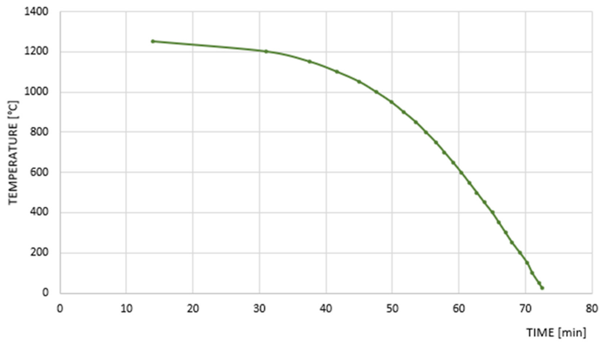
3.1.2. Energy Efficiency Improved Case Results

The equations presented in Section 2.6 were used to obtain the equivalent total heat transfer coefficient h_eq for a billet cooling process within the insulated containers. The value of the equivalent total heat transfer coefficient is 0.0125 [W/m²∙K]. As explained in the Methodology section, the Appendix A code has been modified to consider the two modes of cooling for the billet.

In Figure 9, an example of a cooling process using the containers is represented. In the presented example, the billet is first cooled down in ambient air for 10 min until it is placed within the container for another 20 min. While the billet is still outside, the cooldown begins like in the actual case. After 10 min, the billet is a mixture of liquid parts (the core) and solid parts, as it can be seen in the upper right corner of Figure 9. Like in the actual case, the central part of the billet is horizontal in the graphic because the nodes are still in a liquid state.

From the moment the billet is put inside the container, the heat loss rate of the billet becomes much slower, so the temperature field becomes uniform. After container closure, internal conduction reduces the temperature gradients: cooler surface nodes warm temporarily, while the hotter central nodes cool. The temperature increments of the corner nodes because of the slow cooldown can be clearly noticed in the upper right and lower left images of Figure 9. After 20 min within the container, the billet temperature becomes approximately homogeneous, with a maximum nodal difference below 1 °C. From this point on, the more time the billet is stored within the container, the lower its temperature. However, the temperature of the billet in the inlet of the reheating furnace will be approximately homogenous. Thus, estimating the time and energy required for the reheating of the billets that come out from the containers can be done with the same code as for the actual heating case but with the corresponding initial temperature obtained from the cooling process occurring within the container. Furthermore, it can also be stated that the inner temperature of the whole container will be homogeneous; thus, with just one inner temperature measurement, the temperature of all the billets could be monitored.

The predicted temperature uniformity refers to the equivalent billet representation used in the model. Linear batch scaling remains a first-order approximation. In a real billet pack, the outer billets are more directly exposed to the container walls, whereas the inner billets are partially shielded and exchange heat mainly with neighbouring billets. Gaps, supports, contact resistance, radiation view factors, and loading arrangement may therefore produce nonuniform temperature and heat-loss distributions. A detailed batch model resolving the complete billet pack and container geometry would be required to quantify these spatial effects.

In order to analyse this new cooling process, several possible cases are presented. Different values for the time that the billets are outside and inside the container were analysed, so the influence of these two parameters in the exit temperature of the billets from the containers can be seen (

Table 1. Comparison between different cases for the improved cooling process.

Time Outside the Container	Time Inside the Container	Exit Temperature	Heat Transfer Per Billet
5 min	2 days	1468 $°\mathrm{C}$	304.7 MJ
	5 days	1466 $°\mathrm{C}$	324.0 MJ
	7 days	1465 $°\mathrm{C}$	338.0 MJ
	15 days	1459 $°\mathrm{C}$	392.0 MJ
10 min	2 days	1373 $°\mathrm{C}$	507.8 MJ
	5 days	1352 $°\mathrm{C}$	526.7 MJ
	7 days	1337 $°\mathrm{C}$	539.0 MJ
	15 days	1281 $°\mathrm{C}$	587.0 MJ
15 min	2 days	1192 $°\mathrm{C}$	664.0 MJ
	5 days	1173 $°\mathrm{C}$	680.4 MJ
	7 days	1161 $°\mathrm{C}$	691.1 MJ
	15 days	1112 $°\mathrm{C}$	732.9 MJ
30 min	2 days	863 $°\mathrm{C}$	947.0 MJ
	5 days	850 $°\mathrm{C}$	958.0 MJ
	7 days	841 $°\mathrm{C}$	966.0 MJ
	15 days	806 $°\mathrm{C}$	996.0 MJ

). The total heat exchanged by the billets was also calculated.

The outdoor exposure time strongly influences heat retention in the improved cooling process. The ideal cases of staying outside only for 5 or 10 min are nearly impossible in real life, but the two other cases could be executed.

As shown in Table 1, the exit temperatures of the billets from the containers range from 806 °C to 1468 °C. Figure 10 shows how the billet temperature at the container outlet, corresponding to the reheating-furnace inlet temperature, influences the required reheating time.

Introducing the billets inside the reheating furnace with a higher inlet temperature not only results in time savings but energy savings too. The heat needed to reach 1265 °C is decreased compared to the actual case, meaning less natural gas is required. Using the reheating furnace’s efficiency with a value of 31.10% and knowing that the energy cost of the natural gas is 0.03 €/kWh_LHV, the economic savings for a billet can be obtained.

Table 2. Predicted heat, fuel, reheating-time, and gross fuel-cost savings for the investigated scenarios.

Time Outside the Container	Time Inside the Container	Needed Heat [MJ]	Saved Heat [MJ]	Time in the Furnace [min]	Saved Fuel Consumption [MJLHV and kWhLHV]	Gross Fuel-Cost Saving [€/billet]	Time Saved in Reheating Furnace for Each Billet [min/billet]
Actual case		1064	0.0	72.5	0 MJ	0	0
5 min	2 days	0	1064.0	0	3421.2 ${\mathrm{M}\mathrm{J}}_{\mathrm{L}\mathrm{H}\mathrm{V}}$ = 950 ${\mathrm{k}\mathrm{W}\mathrm{h}}_{\mathrm{L}\mathrm{H}\mathrm{V}}$	28.50	72.5
	5 days	0	1064.0	0	3421.2 ${\mathrm{M}\mathrm{J}}_{\mathrm{L}\mathrm{H}\mathrm{V}}$ = 950 ${\mathrm{k}\mathrm{W}\mathrm{h}}_{\mathrm{L}\mathrm{H}\mathrm{V}}$	28.50	72.5
	7 days	0	1064.0	0	3421.2 ${\mathrm{M}\mathrm{J}}_{\mathrm{L}\mathrm{H}\mathrm{V}}$ = 950 ${\mathrm{k}\mathrm{W}\mathrm{h}}_{\mathrm{L}\mathrm{H}\mathrm{V}}$	28.50	72.5
	15 days	0	1064.0	0	3421.2 ${\mathrm{M}\mathrm{J}}_{\mathrm{L}\mathrm{H}\mathrm{V}}$ = 950 ${\mathrm{k}\mathrm{W}\mathrm{h}}_{\mathrm{L}\mathrm{H}\mathrm{V}}$	28.50	72.5
10 min	2 days	0	1064.0	0	3421.2 ${\mathrm{M}\mathrm{J}}_{\mathrm{L}\mathrm{H}\mathrm{V}}$ = 950 ${\mathrm{k}\mathrm{W}\mathrm{h}}_{\mathrm{L}\mathrm{H}\mathrm{V}}$	28.50	72.5
	5 days	0	1064.0	0	3421.2 ${\mathrm{M}\mathrm{J}}_{\mathrm{L}\mathrm{H}\mathrm{V}}$ = 950 ${\mathrm{k}\mathrm{W}\mathrm{h}}_{\mathrm{L}\mathrm{H}\mathrm{V}}$	28.50	72.5
	7 days	0	1064.0	0	3421.2 ${\mathrm{M}\mathrm{J}}_{\mathrm{L}\mathrm{H}\mathrm{V}}$ = 950 ${\mathrm{k}\mathrm{W}\mathrm{h}}_{\mathrm{L}\mathrm{H}\mathrm{V}}$	28.50	72.5
	15 days	0	1064.0	0	3421.2 ${\mathrm{M}\mathrm{J}}_{\mathrm{L}\mathrm{H}\mathrm{V}}$ = 950 ${\mathrm{k}\mathrm{W}\mathrm{h}}_{\mathrm{L}\mathrm{H}\mathrm{V}}$	28.50	72.5
15 min	2 days	59.9	1004.1	33.33	3228.6 ${\mathrm{M}\mathrm{J}}_{\mathrm{L}\mathrm{H}\mathrm{V}}$ = 897 ${\mathrm{k}\mathrm{W}\mathrm{h}}_{\mathrm{L}\mathrm{H}\mathrm{V}}$	26.90	39.2
	5 days	76.0	988.0	35.00	3176.8 ${\mathrm{M}\mathrm{J}}_{\mathrm{L}\mathrm{H}\mathrm{V}}$ =882 ${\mathrm{k}\mathrm{W}\mathrm{h}}_{\mathrm{L}\mathrm{H}\mathrm{V}}$	26.40	37.5
	7 days	86.0	978.0	35.33	3144.7 ${\mathrm{M}\mathrm{J}}_{\mathrm{L}\mathrm{H}\mathrm{V}}$ = 874 ${\mathrm{k}\mathrm{W}\mathrm{h}}_{\mathrm{L}\mathrm{H}\mathrm{V}}$	26.20	37.2
	15 days	128.0	936.0	39.16	3009 ${\mathrm{M}\mathrm{J}}_{\mathrm{L}\mathrm{H}\mathrm{V}}$ = 836 ${\mathrm{k}\mathrm{W}\mathrm{h}}_{\mathrm{L}\mathrm{H}\mathrm{V}}$	25.00	33.3
30 min	2 days	342.8	721.2	52.50	2318.9 ${\mathrm{M}\mathrm{J}}_{\mathrm{L}\mathrm{H}\mathrm{V}}$ = 644 ${\mathrm{k}\mathrm{W}\mathrm{h}}_{\mathrm{L}\mathrm{H}\mathrm{V}}$	19.32	20
	5 days	354.1	709.9	53.50	2282.6 ${\mathrm{M}\mathrm{J}}_{\mathrm{L}\mathrm{H}\mathrm{V}}$ = 634 ${\mathrm{k}\mathrm{W}\mathrm{h}}_{\mathrm{L}\mathrm{H}\mathrm{V}}$	19.00	19
	7 days	362.0	702.0	53.80	2257.2 ${\mathrm{M}\mathrm{J}}_{\mathrm{L}\mathrm{H}\mathrm{V}}$ = 627 ${\mathrm{k}\mathrm{W}\mathrm{h}}_{\mathrm{L}\mathrm{H}\mathrm{V}}$	18.80	18.7
	15 days	392.0	672.0	54.80	2160.7 ${\mathrm{M}\mathrm{J}}_{\mathrm{L}\mathrm{H}\mathrm{V}}$ = 600 ${\mathrm{k}\mathrm{W}\mathrm{h}}_{\mathrm{L}\mathrm{H}\mathrm{V}}$	18.00	17.7

summarises the data of the savings for each analysed improved cooling–heating process.

As Table 2 presents, when the billets are outside only for five or ten minutes, the reheating-furnace inlet temperature is higher than 1265 °C, meaning that heating up in the furnace is not necessary. Therefore, the time in the reheating furnace and the energy needed to heat up the billets could be completely saved. It can also be noticed that the economic and energy savings are mainly influenced by the time it takes for the billets to be introduced into the containers, with each extra minute the billet is out of the container being crucial.

To finish, the economic savings of having the billets spend less time in the container would be even bigger, since spending less time in the containers means that a smaller number of containers are needed in the factory. In these cases, not only does energy efficiency matter but also good organization of the factory, that is, efficient organization of time and space in the factory is important.

Industrial implementation would depend strongly on crane availability, billet-transfer distance, container positioning, loading and unloading time, and coordination between casting and rolling. The simulations show that delays before container closure substantially reduce the retained temperature and associated savings. The required number of containers would also depend on casting frequency, storage duration, furnace demand, and container turnover.

4. Conclusions

This research work has modelled the actual cooling process the steel billets usually suffer after an electric arc furnace in small- and medium-sized steelworks. This cooling process is usually a free cooling process occurring in an open-air storage area of the factory. If the storage takes more than 24 h, the billets will reach ambient temperature. Then, the billets have to be heated in a reheating furnace to about 1260°C for rolling, where a considerable amount of energy is consumed. For more realistic loading times of 15–30 min, insulated storage reduces the reheating demand by 672–936 MJ per billet and the calculated furnace time by 17.7–33.3 min. The corresponding fuel and gross fuel-cost savings were 600–836 kWh_LHV and EUR 18.0–25.0 per billet, respectively.

These cooling and heating processes were modelled using a two-dimensional transient approach and calculating the billets’ cross-section temperature field by means of the alternating-direction implicit finite difference method. The finite difference simulation code was successfully validated against a hypothetical extremely slow cooling process with a Biot number lower than 0.0001.

The proposed energy, reheating-time and fuel-cost improvement consisted in storing the hot billets as fast as possible in insulated containers just after the billets leave the electric arc furnace. This way, the approximately 36 billets produced in each cast can be stored for several days within the insulated containers. Then, when they are introduced to the reheating furnace, the billets’ temperature should be much higher and could produce considerable energy, time and economic savings.

The results show that insulated storage can provide important improvements to the process. Different cooling and reheating scenarios were analysed by varying the time required to place the billets in the containers and the storage period. The main conclusions are as follows:

• The time the billets are outside the container is the main influencer of the improved cooling process. Therefore, the time it takes to place the billets in the container should be as short as possible.
• The higher the inlet temperature of the billets when put into the reheating furnace, the lower the required time for the billets to be within the reheating furnace, thereby saving time and money, since less time in the furnace means lower fuel expenditure. However, the time to heat up the billet from 25 °C to 1265 °C and from 100 °C to 1265 °C is very similar, which means that the first stage of the heating process does not take much time. When the billet temperature approaches the reheating furnace’s temperature, the temperature increase is much slower. Even so, any saving in the process is an improvement in pursuit of the energy efficiency.
• The containers can retain billet heat for several days. For all the analysed cases, the billet temperature decreased by less than 100 °C during the 15 days of insulated storage. The numerical model predicts that the billet temperature becomes approximately uniform after the initial transient temperature inside the container. However, temperature uniformity across the complete 36-billet batch should be confirmed experimentally.
• The scenarios with outdoor exposure times of 5 and 10 min provide the greatest predicted savings and could eliminate the modelled active reheating requirement. Nevertheless, these loading times may be difficult to achieve under actual plant conditions. The scenarios with loading times of 15 and 30 min also provide substantial energy, time, and gross fuel-cost savings and are considered more realistic for industrial implementation.

From a sustainability perspective, the proposed improvement contributes to reducing fuel consumption in the reheating furnace, which directly implies a reduction in associated CO₂ emissions. Since the reheating stage represents a significant share of the total energy demand in the analysed steelworks, minimizing the required heating through simple thermal management strategies can lead to a noticeable decrease in the environmental impact of the process. Moreover, as the proposed solution is based on passive insulation and does not require complex technological modifications, it can be easily implemented in small- and medium-sized steel plants, supporting a more efficient and sustainable use of energy in the steel industry.

The results should be regarded as preliminary because formal mesh- and time-step-independence analyses and plant-scale experimental validation were not conducted. Other limitations include the use of constant thermophysical properties and furnace efficiency, the simplified container model, and the omission of thermal bridges. The reported monetary values represent gross fuel-cost savings, as container investment, handling, and maintenance costs were not considered.

References

- European Environment Agency (EEA). Final Energy Consumption by Sector and Fuel. Available online: https://www.eea.europa.eu/data-and-maps/indicators/final-energy-consumption-by-sector-9/assessment-4 (accessed on 10 January 2021).
- European Commission. Energy Roadmap 2050. Available online: https://ec.europa.eu/energy/energy2020/roadmap/doc/com_2011_8852_en.pdf (accessed on 10 January 2021).
- Flues, F.; Rübbelke, D.; Vögele, S. An analysis of the economic determinants of energy efficiency in the European iron and steel industry. J. Clean. Prod. 2015, 104, 250–263. [Google Scholar] [CrossRef]
- OECD Publishing and International Energy Agency. Tracking Industrial Energy Efficiency and CO2 Emissions; International Energy Agency: Paris, France, 2007. [Google Scholar] [CrossRef]
- Sarker, T.; Corradetti, R.; Zahan, M. Energy Sources and Carbon Emissions in the Iron and Steel Industry Sector in South Asia. Int. J. Energy Econ. Policy 2013, 3, 30–42. [Google Scholar]
- International Energy Agency. CO2 Emissions from Fuel Combustion Highlights; OECD Publishing: Paris, France, 2017. [Google Scholar]
- Uribe-Soto, W.; Portha, J.-F.; Commenge, J.-M.; Falk, L. A review of thermochemical processes and technologies to use steelworks off-gases. Renew. Sustain. Energy Rev. 2017, 74, 809–823. [Google Scholar] [CrossRef]
- Ramírez-López, A.; Muñoz-Negrón, D.; Palomar-Pardavé, M.; Romero-Romo, M.A.; Gonzalez-Trejo, J. Heat removal analysis on steel billets and slabs produced by continuous casting using numerical simulation. Int. J. Adv. Manuf. Technol. 2017, 93, 1545–1565. [Google Scholar] [CrossRef]
- Choudhary, S.K.; Mazumdar, D.; Ghosh, A. Mathematical-Modeling of Heat-Transfer Phenomena in Continuous-Casting of Steel. ISIJ Int. 1993, 33, 764–774. [Google Scholar] [CrossRef]
- Choudhary, S.K.; Mazumdar, D. Mathematical Modelling of Transport Phenomena in Continuous Casting of Steel. ISIJ Int. 1994, 34, 199–205. [Google Scholar] [CrossRef]
- Geiger, G.H. Transport Phenomena in Metallurgy; Addison Wesley Publishing: Reading, MA, USA, 1987. [Google Scholar]
- Santos, C.A.; Fortaleza, E.L.; Ferreira, C.R.; Spim, J.A.; Garcia, A. A solidification heat transfer model and a neural network based algorithm applied to the continuous casting of steel billets and blooms. Model. Simul. Mater. Sci. Eng. 2005, 13, 1071–1087. [Google Scholar] [CrossRef]
- Dubey, S.K.; Srinivasan, P. Development of three dimensional transient numerical heat conduction model with growth of oxide scale for steel billet reheat simulation. Int. J. Therm. Sci. 2014, 84, 214–227. [Google Scholar] [CrossRef]
- Kakhki, M.E.; Kermanpur, A.; Golozar, M.A. Numerical simulation of continuous cooling of a low alloy steel to predict microstructure and hardness. Model. Simul. Mater. Sci. Eng. 2009, 17, 045007. [Google Scholar] [CrossRef]
- Kim, M.Y. A heat transfer model for the analysis of transient heating of the slab in a direct-fired walking beam type reheating furnace. Int. J. Heat Mass Transf. 2007, 50, 3740–3748. [Google Scholar] [CrossRef]
- Han, S.H.; Baek, S.W.; Kim, M.Y. Transient radiative heating characteristics of slabs in a walking beam type reheating furnace. Int. J. Heat Mass Transf. 2009, 52, 1005–1011. [Google Scholar] [CrossRef]
- Dubey, S.K.; Srinivasan, P. Steel billet reheat simulation with growth of oxide layer and investigation on zone temperature sensitivity. J. Mech. Sci. Technol. 2014, 28, 1113–1124. [Google Scholar] [CrossRef]
- Fujimura, T.; Takeshita, K.; Suzuki, R.O. Mathematical analysis of the solidification behavior of multi-component alloy steel based on the heat- and solute-transfer equations in the liquid–solid zone. Int. J. Heat Mass Transf. 2019, 130, 797–812. [Google Scholar] [CrossRef]
- Seyedein, S.; Hasan, M. A three-dimensional simulation of coupled turbulent flow and macroscopic solidification heat transfer for continuous slab casters. Int. J. Heat Mass Transf. 1997, 40, 4405–4423. [Google Scholar] [CrossRef]
- Yu, Y.; Luo, X. Estimation of heat transfer coefficients and heat flux on the billet surface by an integrated approach. Int. J. Heat Mass Transf. 2015, 90, 645–653. [Google Scholar] [CrossRef]
- Cengel, Y.A.; Ghajar, A.J. Heat and Mass Transfer: Fundamentals and Applications, 5th ed.; McGraw-Hill Education: New York, NY, USA, 2014. [Google Scholar]
- Yang, J.; Xie, Z.; Ning, J.; Liu, W.; Ji, Z. A Framework for Soft Sensing of Liquid Pool Length of Continuous Casting Round Blooms. Metall. Mater. Trans. B 2014, 45, 1545–1556. [Google Scholar] [CrossRef]
- Carnahan, B.; Luther, H.A.; Wilkes, J.O. Numerical Calculation. Methods and Applications; Rueda: Madrid, Spain, 1979. (In Spanish) [Google Scholar]
- Valencia, J.J.; Quested, P.N. Thermophysical properties. In Metals Process Simulation; Furrer, D.U., Semiatin, S.L., Eds.; ASM International: Materials Park, OH, USA, 2010. [Google Scholar] [CrossRef]
- Barnston, A.G. Correspondence among the Correlation, RMSE, and Heidke Forecast Verification Measures; Refinement of the Heidke Score. Weather. Forecast. 1992, 7, 699–709. [Google Scholar] [CrossRef]