Article

A Tool for Carbon Farming Combining Soil Organic Carbon Modelling and Agricultural Decision Support Systems: AresC Model Development and Multi-Case Validation

1
Horta S.r.l., 29122 Piacenza, Italy
2
Research Institute of Nyíregyháza, Institutes for Agricultural Research and Educational Farm, University of Debrecen, 4400 Nyíregyháza, Hungary
*
Author to whom correspondence should be addressed.
Sustainability 2026, 18(15), 7879; https://doi.org/10.3390/su18157879
Submission received: 29 May 2026 / Revised: 16 July 2026 / Accepted: 17 July 2026 / Published: 4 August 2026

Abstract

Increasing soil organic carbon (SOC) is widely recognized as a key pathway for climate change mitigation and enhancing soil ecosystem services, but additional carbon farming practices can lead to additional GHG emissions. We propose a process-based SOC module, AresC model, integrated into an agronomic DSS already in use to monitor SOC while optimizing crop management practices and GHG emissions. AresC model estimates SOC dynamics simulating the effects of management practices, including soil tillage, under Mediterranean climatic conditions. The integrated DSS-SOC model is tested in four case studies including arable crops and orchards under different conditions, with a focus on arid Mediterranean areas. The AresC model showed good agreement with the measured values in all conditions with no significant bias or root mean square errors, and Spearman correlation factors very close to 1. A global sensitivity analysis showed that carbon inputs are the dominant driver of SOC. Finally, compared to the RothC model, AresC showed better performance under drier conditions, and no significant differences were observed between the two models in humid conditions. This study, therefore, demonstrates the potential in agricultural carbon accounting applications of the newly developed AresC model integrated into an agronomic DSS to optimize crop management while properly simulating SOC dynamics.

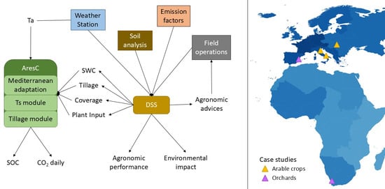
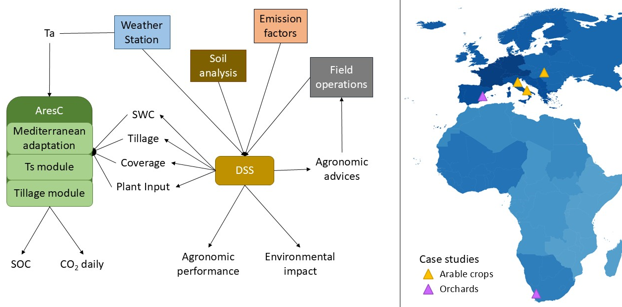
Graphical Abstract

1. Introduction

Sustainable development planning in agricultural landscapes should incorporate carbon farming practices [1,2], since an increase in soil organic carbon (SOC) not only reduces atmospheric levels of CO2 [3] but also enhances many soil ecosystem services [4,5,6]. The potential to increase SOC in agricultural soils is especially high in Mediterranean areas and arid ecosystems [6]; however, different practices have varying efficacies depending on the agronomic context in which they are introduced (soil type, weather conditions, type of production, etc. [7]). Moreover, the use of these practices may lead to an increase in field operations, thus resulting in an increase in total GHG emissions [8], and may also affect overall agricultural yields [9]. To support farmers and policymakers in selecting the most suitable practices to integrate in their activities for balanced crop production, climate change mitigation and sustainability, a decision support system that integrates agronomic management advice with a dynamic SOC model may be a viable option [10].
Agronomic DSSes are computer-based information systems designed to provide farm-level advice for the optimization of production and minimization of environmental impacts [11,12]. They analyze large volumes of data using databases, mathematical equations and models, with the aim of simplifying the decision-making process [13] for the user. They consist of multiple interlinked models that represent the ecosystem and have been widely tested and vetted for carbon accounting purposes [14]. The models used in the DSSes can either be data driven or process-based. In the first instance, the DSS makes statistical inference from large numbers of observations or datasets to identify practices that have worked and performed well in similar conditions in the past. In the second case, the DSS uses field-specific inputs together with biological, physics and chemical models to estimate the response of the system (soil and crop) to certain practices [15]. While a process-based DSS may have its challenges [15], its structure makes it straightforward to include a process-based SOC model, thus helping to evaluate the effects of a certain agricultural practice on yields, GHG emissions and SOC stock all at once.
Process-based SOC models simulate the incorporation of organic matter into the soil, its decomposition and degradation and the eventual formation of CO2, which is then released from the soil through respiration [16]. As such, SOC models assess both the changes in SOC stock and CO2 emission from the soil. The SOC is simulated as different pools, differentiated by their degradation rates, which can be modified by soil conditions (soil temperature, soil water content, etc.), plant coverage, type of biomass added to the soil, and soil characteristics (e.g., clay content; [17]). Existing SOC models differ in the level of detail they represent, the definition of the SOC pools, and the equations used to simulate the organic matter degradation [16]. RothC [18], Century [19], and the SOC module in APSIM [20] are examples of widely used SOC models. RothC and Century are used as examples by FAO for modelling carbon dynamics in soils [21,22]. RothC is a very simple model, with a bulk soil model (no subdivision in different soil layers) and no module to simulate the growth of vegetation and the resulting carbon input. Century is a more complex model, taking into account soil layers, leaching, other nutrients, modules for the growth of the vegetation, etc. RothC’s simplicity and flexibility make it a suitable model for developing a SOC module to be integrated into a DSS. RothC was included in the FullCAM a calculation tool for modelling Australia’s greenhouse gas emissions from the land sector [23] (as discussed in the accompanying article “A tool for Carbon Farming combining Soil Organic Carbon modelling and Agricultural Decision Support Systems: adapting the RothC model to simulate DSS informed agricultural practices in a Mediterranean climate”).
Examples of DSSs that are already incorporating SOC models include: APSIM, DSSAT, COMET-Farm and FullCAM [24,25,26,27,28]. These DSSs can be used to estimate the changes in SOC and GHG emissions depending on the ecological conditions simulated. With the exception of COMET-Farm, none of these DSSs emphasizes the link between cropping management and climate change mitigation [14,24,25,28,29]. COMET-Farm was specifically designed to help both policy makers and farmers simulate agricultural land management practices; however, it is very data demanding, and its application is limited by its reliance on USDA national inventories and surveys to estimate soil and crop management [30]. Similarly, FullCAM integrates Australian databases in its structure [31]. Integrated systems estimating SOC directly embedded within a DSS for the simultaneous optimization of sustainability and agronomic production exist only in the USA. Such a system is lacking in Europe due to fragmented governance and soil databases, which is especially problematic for semi-arid and Mediterranean regions where soils are depleted in SOC. Additionally, no customizable tool exists for different end-users (farmers, supply chains, policy makers). This integration has the potential to enable carbon accounting without compromising food production.
To address these gaps, we propose a process-based SOC module called AresC, built for integration into an agronomic DSS already in use for the estimation of GHG emissions and optimization of agronomic productivity. The objectives of this study were to (a) develop the AresC model for integration into the agronomic DSS to additionally estimate SOC; (b) validate the integrated DSS-SOC model in four long-term case studies to test its ability to represent different climatic conditions and agricultural systems, with a focus on arid Mediterranean areas; and (c) compare the performance of the AresC model against the widely used RothC model.
This study first presents AresC and the agronomic DSS into which it was integrated. We then describe the four case studies considered and explain the simulation setup. Finally, we show the comparison between observed data with simulations generated by agronomic DSS and AresC against RothC (version 26.3 [18]).

2. Materials and Methods

2.1. DSS-SOC Model Integration Framework

2.1.1. The Agronomic DSS

The system presented here is a decision support system, or DSS, for managing agricultural fields. It is based on the private infrastructure of Horta S.r.l. presented by Rossi et al. in 2010 [11] and available at the web page https://www.horta-srl.it/en/ (accessed on 27 May 2026). The DSS collects data from various sources, processes it using mathematical equations and provides management advice and reports, as shown in the flow chart in Figure 1. Data inputs cover aspects such as weather, soil, crops, and activities undertaken in the field. These are sourced from sensors such as weather stations and soil sensors, soil analysis, satellite maps, and users, who report on field description and management history. This information is stored in databases and standardized to make it compactible with different applications. The databases include standard GHG emission factors, plant biomass allocation, plant stress response and nutrient management, and soil hydraulic properties. They serve as input sources for mathematical models designed to optimize agronomic and sustainable performance with minimum material inputs. These models consider factors such as nutrition, plant diseases, insect pressure, irrigation, crop phenology, and yield. By consulting crop-specific agronomic recommendations during the cropping season, users take informed actions and update the list of operations carried out in the field.
At the end of the agronomic season, the DSS provides performance indicators in the form of lists, charts, or reports. Some of these indicators reflect the environmental impact of the specific crop management applied. The sustainability indicators are produced using a LCA (Life Cycle Assessment) approach “from cradle to field gate”, so that all materials and energy used on field are accounted from the production of raw materials to the delivery of the final agronomic product to the next step in the food value chain (storage or processor). These indicators comply with the standards ISO 14040 [32], ISO 14067 [33] and EPD standards. The assessment includes different impact endpoints, such as biodiversity, air pollution, and human health. A PEF indicator called “Climate Change” [34,35] provides insights on the agronomic carbon cycle, estimating CO2 equivalent emissions from all inputs or outputs. The AresC model, described below in Section 2.1.2, was integrated into the DSS to improve reporting on ecosystem services and GHG emissions. Soil organic carbon (SOC) sequestration is estimated using the AresC balance, while soil CO2 emissions are derived from AresC simulation of soil heterotrophic respiration (see Figure 1). Daily SOC from AresC is also used to update the soil organic matter parameter in the database, which is widely used by other models in the DSS.

2.1.2. The AresC Model

The AresC model is a process-based model that simulates daily SOC dynamics in agricultural soils. It estimates both daily SOC content and CO2 emissions in non-waterlogged soil. The modelled SOC is divided into 4 pools that degrade at different turnover rates, with first-degree kinetics. The amount of C that decomposes from any pool in one day i (Yi) follows the exponential decay function in Equation (1):
Yi = Yi−1 (1 − e −a b c ST k (1/365))
where Yi−1 is the initial amount of C; a, b and c are the factors that modify the degradation speed according to soil temperature, soil water content and soil live coverage, respectively; ST is the modifying factor for the soil tillage; k is the turnover rate of the pool; and 1/365 stands for the daily timestep.
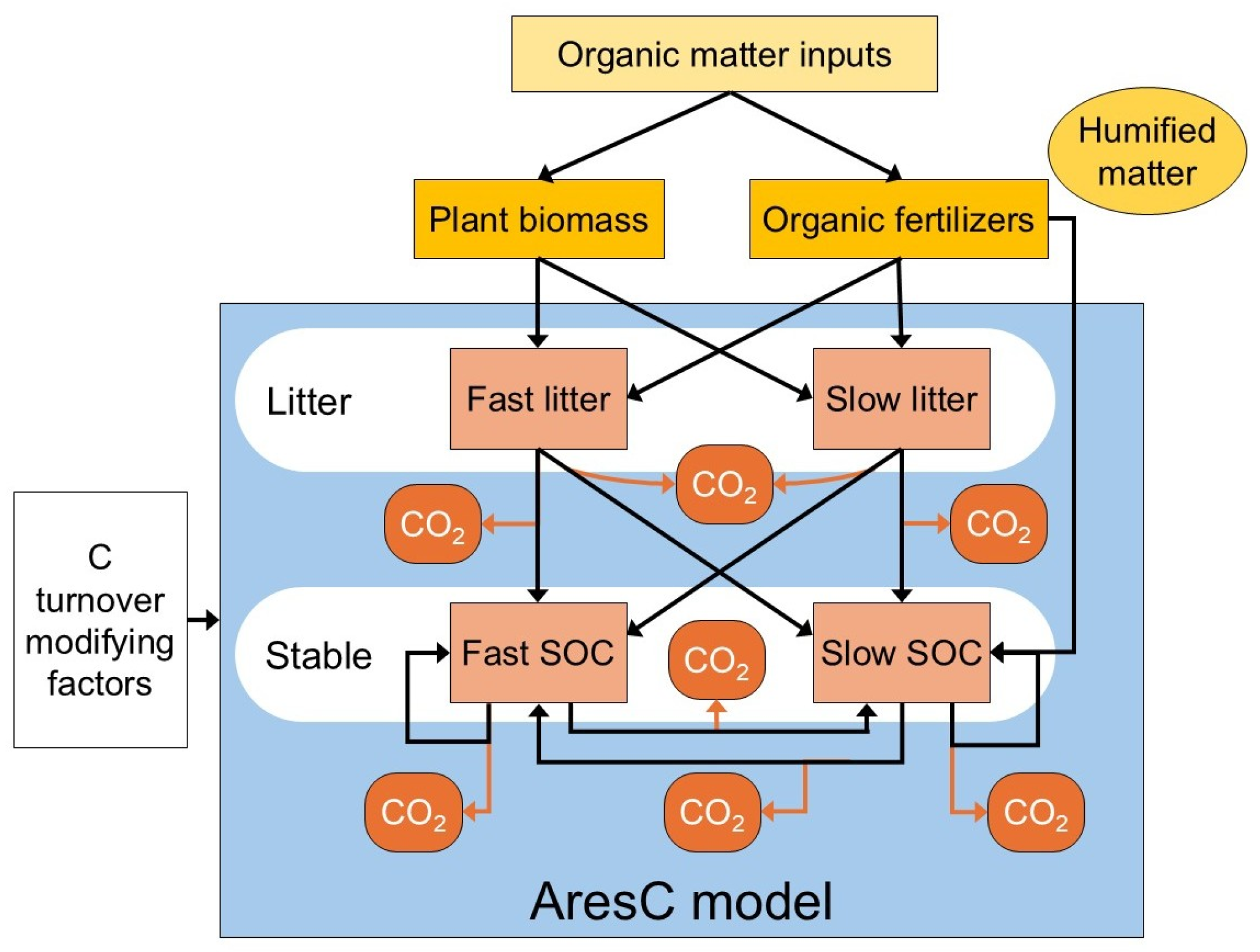
The carbon pools from faster to slower degradation rate are called Fast litter, Fast SOC, Slow litter, and Slow SOC, respectively with a residence time of 0.1, 1.5, 3.3 and 20 years. Carbon (C) flux among the pools is shown in Figure 2. Organic matter inputs to the soil come from plant biomass or organic amendments and fertilizers. They are defined from user-recorded data such as field operations, crop yields and applied fertilizers. The aboveground and belowground biomass of plants is determined using allometric equations that incorporate harvest index and shoot:root ratio [28,36,37,38,39,40,41]. All plant biomass is assumed to have a carbon content of 45% [36,42].
C inputs from plants are divided between the two litter pools according to their affinity for degradation, which is linked to the C:N ratio of the material. Woody plant material is mostly allocated to the Slow litter pool, while leafy plant material is mostly allocated to the Fast litter pool. Organic fertilizers are more advanced in the degradation process than plant biomass. Hence, the C from organic fertilizers is allocated to Fast litter, Slow litter and, depending on the percentage of humified matter, Slow SOC. The RothC model allocates the farmyard manure in a similar way [18], and Mondini et al. improved significantly its simulations by allocating all exogenous organic matter (i.e., organic amendments and fertilizers) to the stable pool using the humified content [43]. In AresC, the humified matter content is set as 2% of the quantity of organic matter in fertilizers, like in RothC farmyard manure, or it is updated with data from specific labels or chemical analysis.
The C in the litter pools moves to Fast SOC and Slow SOC pools, which are the stable pools. Here, carbon can shift to the other stable pool, or it can remain in the initial pool. At every C turnover from any pool, a fraction undergoes mineralization, and CO2 gaseous emissions are produced based on the soil clay content. These CO2 emissions are at the basis of SOC dynamics modelling [18,44,45]. The sum of CO2 emissions from all pools in one timestep accounts for daily soil respiration or heterogenic respiration. The quantity of C in all pools at each timestep forms the daily SOC.
The C turnover rate of a pool (k in Equation (1)) determines its degradation speed. Modifications to the turnover rates are determined by the agronomic management through the effects of soil water content, soil temperature, live soil coverage and soil disturbance, as shown in Figure 1.
Estimates of soil water content are based on the crop-specific water balance model included in the DSS, a bucket model as in FAO Irrigation and Drainage Paper No. 56 [46]. The water balance model includes the effect of crop development, proximity to the groundwater table, irrigation, soil characteristics, and weather conditions. The water content is driven by precipitation and soil potential evaporation calculated using hourly weather data. The parameters for soil water transfer are calculated using Van Genuchten formulation [47]. Thanks to the soil being allowed to dry up until the capillary water content, the water balance model includes drought effects on plants and soil. Soil temperature is estimated from air temperature, measured hourly at 2 m height, applying an analytical function to estimate the heat transfer from air to soil in wet soil, as in Bittelli et al. 2015 [48].
AresC considers the effect of soil coverage (e.g., by cover crops) and soil tillage operations. Plant soil coverage accounts for root priming that can affect microbial activity when live roots are present in soil. The factor for live soil coverage indicates if the soil is vegetated or bare, as modelled in RothC [18]. The effect of soil tillage is a combination of the depth reached by the soil disturbance, which is an indicator of the tillage intensity, and the mean air temperature. These two factors have been identified as the main drivers of the effect of soil tillage on SOC degradation [49,50]. Soil tillage in AresC is modelled as a linear function to simplify processes. The tillage factor reaches its maximum magnitude on the day of the operation and decreases within a 30-day period. If there is more than one tillage event within this period, the higher effect is predominant, since mixing the soil layer that has already been tilled has no effect.
The soil tillage effect and the degradation rates of the pools were calibrated using SOC and GHG emission datasets from an 8-year long trial in Ravenna (Italy). Only two of the eight experimental plots were included in the calibration, while the remaining six were used for model testing. The calibration and the initial model testing are described in the accompanying paper, which is under publication: “A tool for Carbon Farming combining Soil Organic Carbon modelling and Agricultural Decision Support Systems: adapting the RothC model to simulate DSS informed agricultural practices in a Mediterranean climate”.
Table 1 compares the AresC model with some of the most used SOC models: RothC, the SOC module in APSIM, and Century. The AresC and RothC models represent only the SOC dynamics, while the SOC calculations in APSIM and in Century are performed by modules embedded in complex systems that represent the whole agroecosystem. AresC is integrated into an agricultural DSS for the optimization of agricultural productions, like APSIM and Century. Moreover, the AresC and APSIM simulations have a daily timestep, while the RothC and Century models have a monthly timestep. The modelled soil includes only a single layer in both the AresC and RothC models, while five and two layers or more are included in the APSIM and Century models, respectively. Consequently, the AresC and RothC models generally require a lower amount of data compared to the APSIM and Century models.
SOC dynamics in the AresC model are represented using four pools, which is within average compared to five pools in the RothC and Century models and three pools in the APSIM model. A high number of pools can increase equifinality issues in SOC estimation [36]. The soil water content is estimated using bucket models. For the AresC model, it is run within the DSS and it follows FAO guidelines, accounting also for the water table level and capillary rise. The water balance in RothC is simpler, while in both APSIM SoilWat [51] and Century the bucket model is divided into different soil layers. The soil temperature in both the AresC and APSIM models is estimated through simplified heat transfer equations, while in the RothC and Century models the air temperature and soil surface temperature, respectively, are used without elaboration. In all models, the SOC dynamics include the soil tillage effect, except for RothC. AresC was explicitly adapted to represent semi-arid conditions, while APSIM and Century account for them implicitly, having been developed to represent Australian and Southwest USA climatic conditions.

2.2. Case Studies

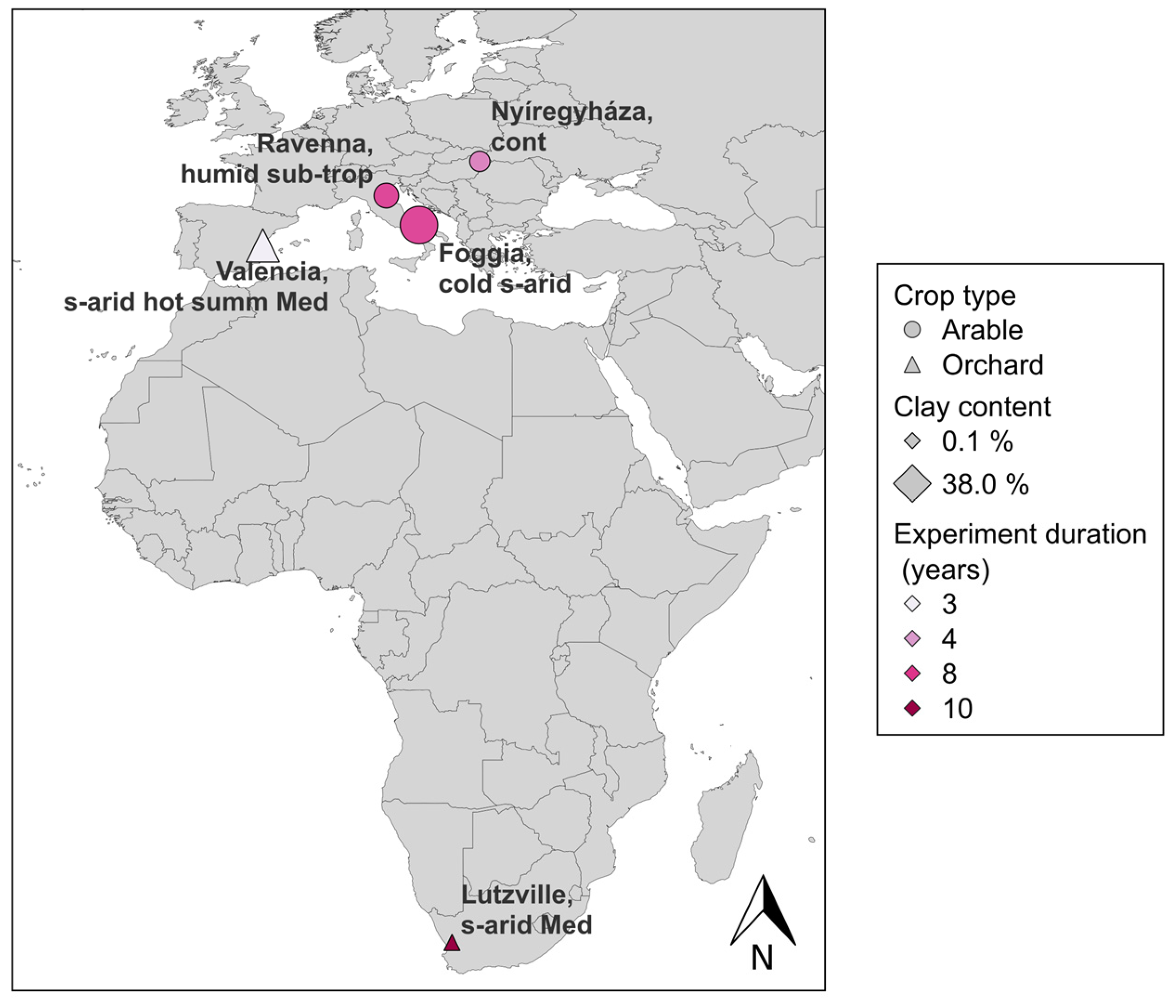
The integration of the AresC model into the agronomic DSS was tested and evaluated using four long-term studies from the literature, from six distinct sites, as shown in Table 2 and in Figure 3. We selected studies with long term datasets of SOC (3 years minimum, at least 3 SOC measurements, see Table 2) where the use of a certain practice (cover crop, intercropping, mulching) is tested against a control plot. We also included studies with both arable crops and orchards. The sites selected were: Foggia and Ravenna, Italy [55,56,57], Nyíregyháza, Hungary [58,59], Lutzville, South Africa [60,61,62], and Valencia, Spain [63,64]. Foggia and Ravenna were chosen to test model calibration, as described in the accompanying article “A tool for Carbon Farming combining Soil Organic Carbon modelling and Agricultural Decision Support Systems: adapting the RothC model to simulate DSS informed agricultural practices in a Mediterranean climate”. The two plots in Ravenna used for the calibration were excluded to ensure an independent validation. Nyíregyháza, Lutzville, and Valencia were chosen because they represent a range of climates, spanning from continental to arid climates, and have orchards and arable crops. All cover crops included in the experiments serve as green manure, and the resulting biomass is a C input into the soil.

2.2.1. Ravenna and Foggia, Italy [55,56,57]

The AresC model was tested in two locations in Italy: Foggia (41°29′27″ N, 15°30′14″ E) and Ravenna (44°29′15″ N, 12°10′44″ E). According to the Koppen–Geiger classification, the climate in Foggia is cold semi-arid [65]. The soil is classified as Vertisol under both WRB and USDA methodologies [66,67], with mainly silty clay loam texture. In Ravenna the climate is humid sub-tropical [68], and the soil is classified as Cambisol under WRB [65] or Inceptisol under USDA [67] with a silty clay loam texture.
The dataset includes 8 years (2018 to 2025) of experiment and compares two management systems with local intensive crop rotations. ECS treatments (Efficient Cropping System) apply agronomic advice from the DSS and include cover crops and N-fixing crops into the rotations, while CCS treatments (Conventional Cropping System) are managed by local farmers and practices. In every site, four ECS plots are alternated with four CCS plots, each 1 ha wide. Direct observations are available from comprehensive soil samplings, weather stations and crop samplings. Further trial description is in the accompanying paper under publication “A tool for Carbon Farming combining Soil Organic Carbon modelling and Agricultural Decision Support Systems: adapting the RothC model to simulate DSS informed agricultural practices in a Mediterranean climate”. In this paper, the SOC results from observations and simulations are averaged according to the management to detect the differences between ECS and CCS.

2.2.2. Nyíregyháza, Hungary [58,59]

The Hungarian experiment is located in Nyíregyháza (47°58′35″ N, 21°41′50″ E) at the Research Institute of Nyíregyháza Institutes for Agricultural Research and Educational Farm of the University of Debrecen. According to Koppen–Geiger weather classification [68], the climate is continental with hot summers and increasingly frequent summer drought periods due to climate change. The soil is humic sand, classified as Arenosol under WRB [66] and Entisol under USDA [67]. The experiment studied the impact of cover crops in a crop rotation system typical of Hungary, and the dataset spans four cropping seasons, from 2019 to 2023. The experiment included four rotations (R1 to R4) with common crops found in Hungary’s productive areas: triticale, oats, and maize. Additional soil coverage was implemented with four cover crop treatments: white lupine (Lupinus albus), common vetch (Vicia sativa), oil radish (Raphanus sativus convar. oleiferus), and buckwheat (Fagopyrum esculentum). The biomass of the cover crops was incorporated into the soil during the autumn period.
Control treatments were mineral-fertilized and unfertilized, without cover crop application. Direct observations were available from soil sampling, daily weather data, and the commercial yield or dry matter production of the cover crops. Each of the six treatments was simulated in all four rotations, and the resulting SOC was averaged according to the rotation.

2.2.3. Lutzville, South Africa [60,61,62]

The Lutzville experiment took place from 1993 to 2002 in the Olifant River Valley, South Africa (31°34′60″ S, 18°52′0″ E). The area has a semi-arid climate, according to Koppen–Geiger classification [68], and sandy soil classified as Cambisol under WRB [66] or Inceptisol under USDA [67]. The experiment monitored the effects of cover crop species and management practices on the soil of a Sauvignon Blanc/Ramsey vineyard. The cover crops used were Vicia dasycarpa Ten. (grazing vetch), Medicago truncatula Gaertn (“Parabinga” medic), Avena sativa L. (“Overberg” oats), Medicago truncatula Gaertn (“Paraggio” medic), Avena strigosa L. (“Saia” oats), Ornithopus sativus L. (pink Seradella), and Secale cereale L. (rye). The cover crops were terminated every year using chemical control in September (BB management) or in November, skipping years 1995, 1997 and 1999 (AB management). This study includes seven BB and seven AB treatments, for a total of fourteen treatments. We excluded mechanical control due to limited replications and datasets.
Direct observations of SOC [61] and dry matter production [60] of the cover crops were used as model inputs. Since rainfall and irrigation data were only available for the growing season, and there were no available weather stations in the area, we used meteorological data from Copernicus Climate Change Service [69]. The SOC resulting from the fourteen treatments was averaged according to the management applied (BB and AB) and according to the cover crop species.

2.2.4. Valencia, Spain [63,64]

The experiments in Valencia, Spain, are located within a 30 km radius in two citrus orchards, in Paiporta (P, 39°25′2″ N, 0°25′4″ W) and in Sueca (S, 39°12′36″ N, 0°18′23″ W). According to Koppen–Geiger classification [67], the climate is semi-arid hot summer Mediterranean. In Paiporta, the soil is classified as Typic Calcixerept under USDA [67] or Cambisol under WRB [66] with a clay loam texture, and in Sueca, it is classified as Oxyaquic Xerofluvent under USDA [67] or Fluvisol under WRB [66] with a silty clay loam texture. From 2019 to 2022, two plots at each site were covered with straw mulch (M), and two plots were left with bare soil as a control (B). The inputs for the simulations are the same as those used for the RothC simulations published in the dataset by Visconti et al. [64].

2.3. Setup of the AresC Simulations

Inputs for the AresC model and the DSS, including the soil water balance, were defined using data from soil samplings, weather station datasets, and crop samplings. The minimum weather inputs were precipitation and air temperature. The minimal soil data requirements include USDA texture, organic matter content, bulk density, and coarse fraction. For the crops, C inputs to soil are estimated with the allometric equations described in Section 2.1.2, using at minimum the crop species, dry weight of the yield, and an indication of the cover crop growth level.
All minimum information required by the DSS and the AresC model was available for the Foggia, Ravenna and Nyíregyháza sites. Dry weights of crop residues were also available for all experiments. In Ravenna and Foggia, biomass production and their C content were directly measured from crop samples. For the Lutzville case study, soil bulk density for the 0–30 cm soil layer, soil coarse fraction and weather trends were missing (only total water dosage was available for the growing season). These gaps were filled using the accredited ISRIC SOTER dataset [70] and Copernicus Climate Change Service [69]. For the Valencia case study, all inputs, including soil water content and C inputs, were obtained from RothC simulations, and no further data elaboration was required.
The simulations have been initialized using spin up runs to determine the relative relevance of each carbon pool. The initial SOC in the simulation was adjusted using the first measurement of SOC in the modelled study plot [63,71]. In Lutzville, the initial SOC corresponded without any adjustment. SOC data was converted to tC ha−1 using bulk density. The simulations considered the same soil layer of the soil samplings, which was 0–30 cm for all simulations, apart from the Valencia case study, where soil was sampled in a 0–20 cm soil layer.
AresC and RothC [18] simulations were run using the same inputs for both models, in each treatment–site combination. Once the model inputs had been defined, they were converted from daily to monthly, since the timestep is daily in AresC and monthly in RothC. The Supplementary Materials contain detailed data on soil and leafy C inputs used in all simulations.

2.4. Statistical Analysis

Since one of the objectives of this study is to test the ability of the AresC model to represent the effects of different cropping managements, SOC datasets are averaged according to the agronomic managements, as explained above. The exception is the Valencia experiment, where replicates of the management in the same field are not available.
We tested the ability of AresC and RothC models to represent the observed SOC using the root mean square error (RMSE) in percentage [72]. This statistic highlights the relative difference between observed and predicted values, weighted as a percentage of the mean value of observed data. The smaller the difference between observed and simulated values, the closer the value is to zero.
The simulations were grouped together and analyzed using the following statistics:
  • Model efficiency, EF [72], was estimated for each site, in order to increase the degrees of freedom and the robustness of the analysis. EF ranges from 1 to minus infinite. Positive values indicate that the model better estimates the trend in the measured values than the average of all observations. Negative values mean that the average of all observations is a better estimate of the trend.
  • Mean difference, MD [72], represents the bias of the model compared to the observations and can show over- or underestimation if positive or negative, respectively. MD is equal to zero when the observed and predicted values correspond.
  • Relative error, E [72], is the preferred bias measurement when replicates are available.
  • Normalized mean square error, NMSE [42], is similar to RMSE, but the normalization is added to compare different levels of soil C. This value is unbiased towards overestimation or underestimation.
  • Spearman rank correlation, rs [42], is an non-parametric measure of the correlation between two sets of variables (in this case observed and predicted), including non-linear associations. The maximum rs value is 1, indicating full positive correlations, and minimum value is −1, indicating full negative correlation. The worst value for a model is 0, indicating no correlation.
  • Student’s t-test is used to determine whether the RMSE and the bias (MD and E) are significant [72].
MD was applied to the Valencian site only since replications of SOC measurements are not available in the literature. In all other cases, we used E. We also compared the quality of AresC and RothC estimates, dividing the dataset into two groups, orchards and arable crops, and applying MD, E, NMSE, and rs. Since the SOC on the first soil observation was used to initialize the model, it was discarded from all statistical analysis.
Finally, we conducted a global sensitivity analysis on the AresC model to understand the effects of input variability on the variance of the results. A Monte Carlo simulation (10,000 simulations) was used to calculate the first-order variance-based Sensitivity Indices [73]. More information is included in Appendix A.

3. Results and Discussion

SOC observations and simulations of the AresC and RothC models are shown in Figure 4, Figure 5 and Figure 6. Results from the statistical analysis are shown in Table 3, Table 4 and Table 5. The Supplementary Materials contain the comprehensive dataset of measured SOC with the relative standard deviation, and the simulated SOC of the Lutzville site averaged for the cover crop applied.

3.1. Comparison Between AresC and Observations

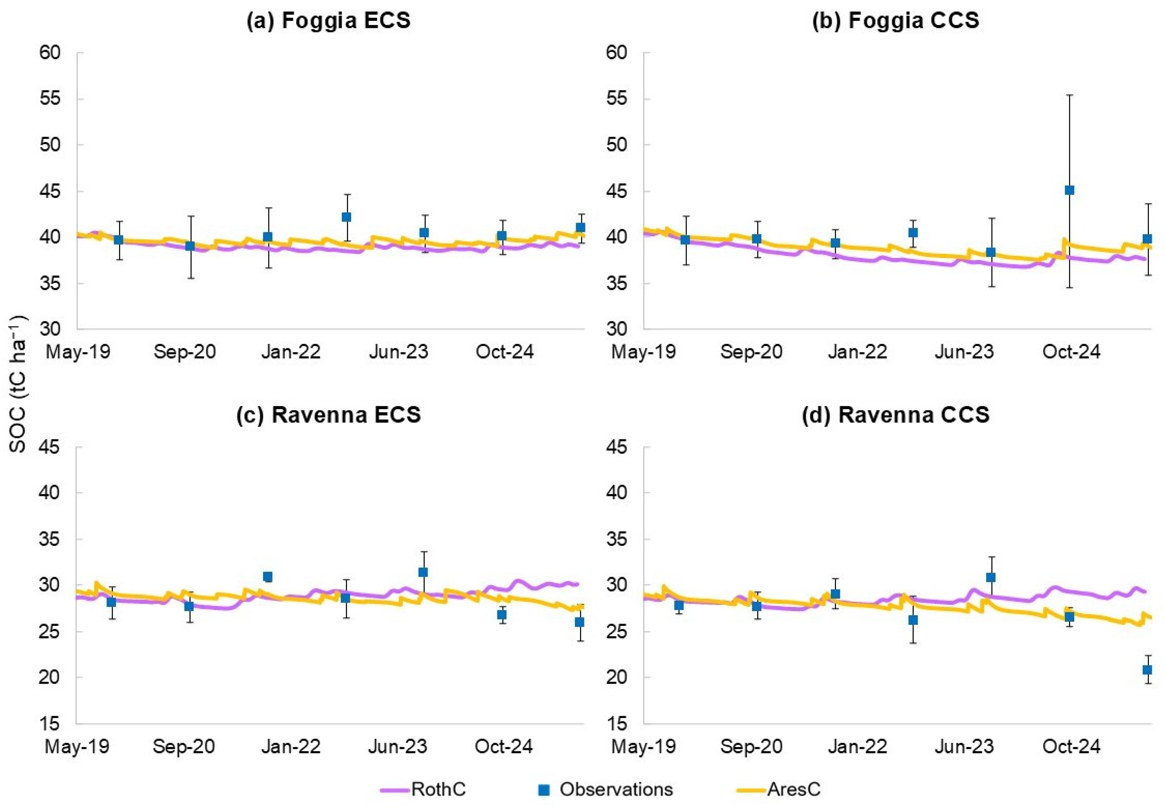
In Foggia site (Italy), the measured SOC trend is stable (Figure 4a,b). The changes over the 8-year period are 1.26 tC ha−1 in ECS and 0.08 tC ha−1 in CCS. The AresC model estimates follow the SOC trend in the observations. RMSE values shown in Table 3 are small, 3.2% and 6.2% in ECS and CCS respectively, and not significant according to Student’s t-test. In the Ravenna site (Italy, Figure 4c,d), SOC was mostly stable, with a slight decrease in the last two observations. The AresC model followed the observed trend, including the slight decrease in SOC in the last two years. Only the last measurement in CCS in Ravenna is clearly out of the observed standard deviation. Over the 8-year period, the observed SOC decreased by −2.11 tC ha−1 in ECS and −6.95 tC ha−1 in CCS, compared to −1.38 tC ha−1 and −2.04 tC ha−1, respectively, estimated by AresC. RMSE values are small, 5.0% and 11.0% respectively, and not significant.
Considering both Italian sites, EF shows that AresC simulations are a better SOC estimation than the average of all measures, with a slight overestimation indicated by the relative error E (2.7% in Foggia and 1.5% in Ravenna), which is not significant. Overall, RMSE in the Foggia plots (6.6%) is smaller compared to Ravenna (10.0%). We expected a better fit in Ravenna, since the calibration used for AresC’s soil dynamics was done on datasets from the Ravenna experiment (as mentioned above in Section 2.1.2 and Section 2.2.1); nevertheless, both bias and RMSE are not statistically significant.
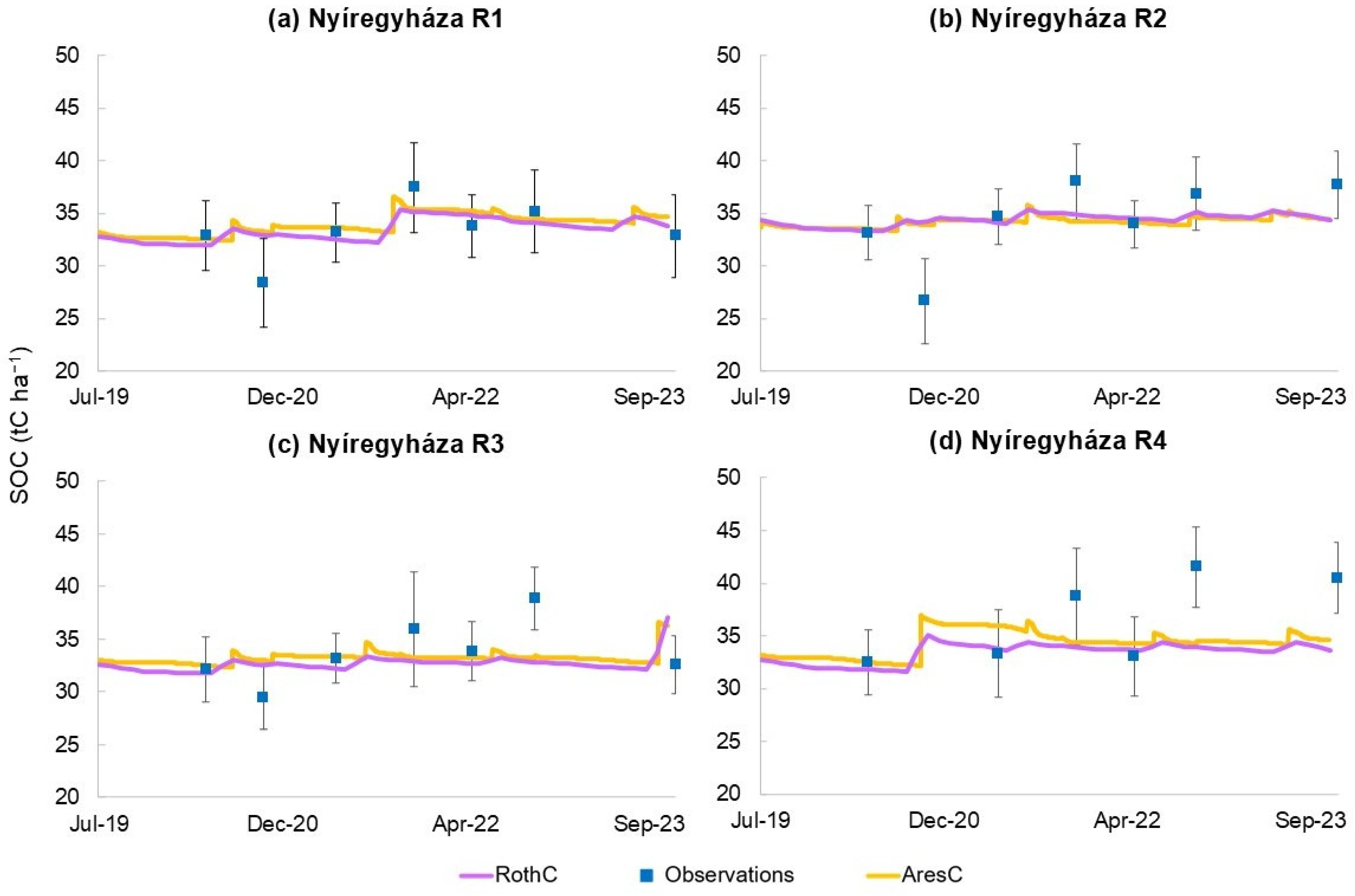
At the Nyíregyháza (Hungary) site, all measured SOC, shown in Figure 5, highlights an increase during the 4-year period that reaches the highest in rotation 4 with a +8 tC ha−1, and the lowest in rotation 1 with a more stable trend. Overall, AresC estimates follow the measured trend, but they overestimate SOC in the last soil sampling in rotation 1 and 3, while it underestimates SOC in rotations 2 and 4. In rotation 4, observations show a clearly increasing trend that could not be simulated. However, RMSE values remain minimal (Table 3), ranging from 6.9% in rotation 1 to 12.2% in rotation 4, and small bias (1.5%). Both RMSE and bias are not statistically significant. EF is positive (0.3).
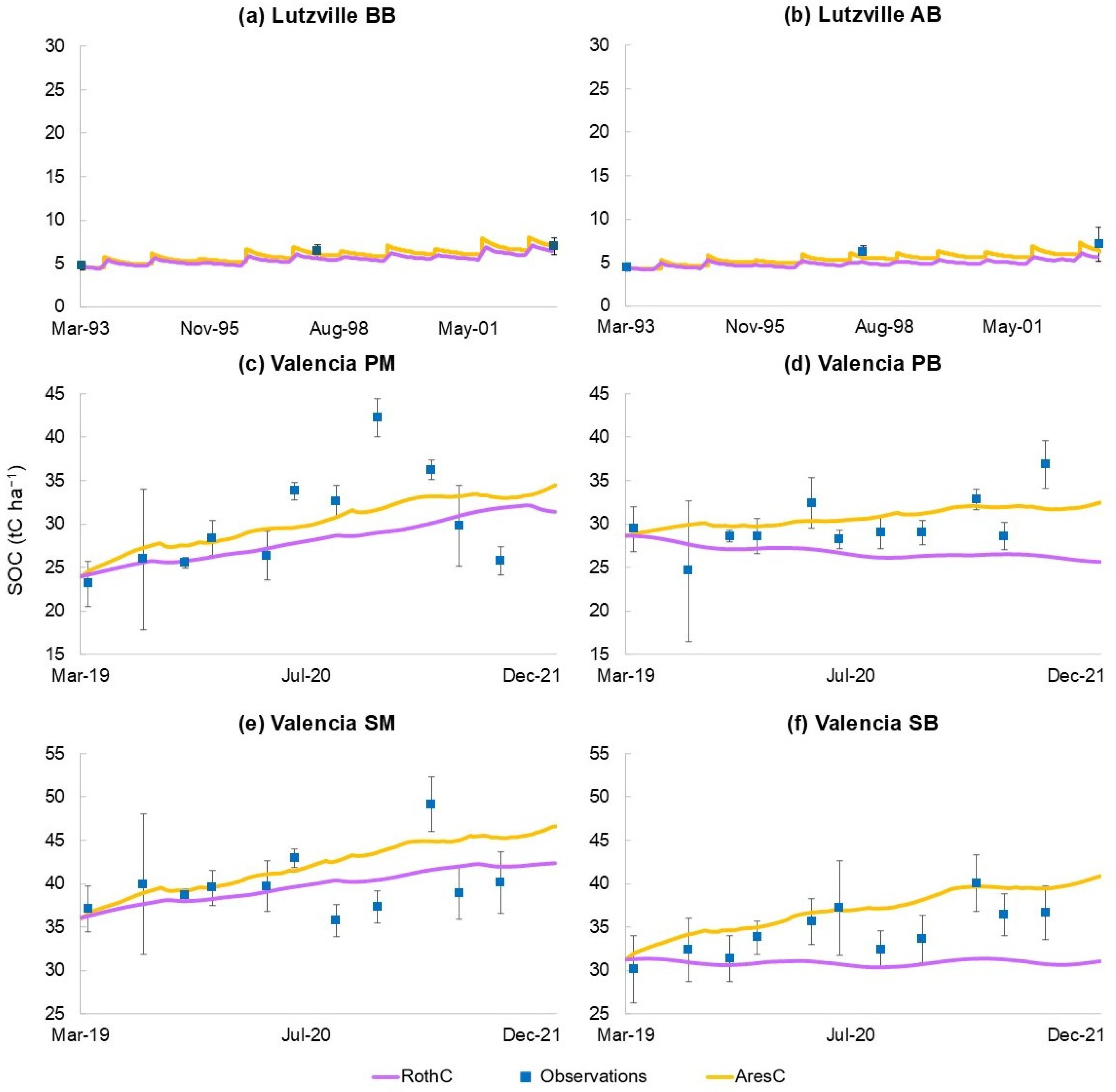
At Lutzville (South Africa, Figure 6a,b), the SOC observations show minor changes over the ten-year period, corresponding to an additional 2.35 tC ha−1 and 2.70 tC ha−1 in BB and AB, respectively. The AresC model follows this trend, showing low RMSE values of 3.5% and 10.1% in BB and AB respectively (Table 4), which are not statistically significant. The AresC model detects the effect of cover crop species, since the simulation follows the observed trend in Figure S1. The SOC measured in grazing vetch plots increased by 3.95 tC ha−1 over ten years, which is the highest compared to the other cover crop species. It is also about double the simulated amount, i.e., 1.85 tC ha−1. Nevertheless, this increase is not reflected in the biomass input (average of the yearly dry weight), which is below average at 2.29 t ha−1 for BB grazing vetch and 2.09 t ha−1 for AB grazing vetch compared to 2.41 t ha−1 for all cover crops. Uncontrolled factors could be involved.
The RMSE values are higher for cover crop average simulations compared to management average, ranging from 4.7% for pink Seradella to 22.8% for grazing vetch. However, none of the RMSE values are significant. The RMSE in percentage corresponds to minimal absolute values compared to the other case studies. Lutzville sandy soils are very poor in organic matter. The initial SOC in 1993 was only 4.43 tC ha−1 on average. The simulation overestimated SOC, with a bias of 6.3%, also not significant. Moreover, soil sampling in Lutzville consisted of three measurements for each of the 14 treatments, over the 10-year period. Since the first measurement was discarded in this statistical analysis, the dataset used in each plot included only two measurements for each treatment. This could seriously limit the study, affecting the detectability of SOC trends in this experiment despite the long period. To address this, we used averaged data that included seven replications each for BB and AB management and two replications each for cover crop species.
In the Paiporta and Sueca case studies (Figure 6c–f), the observed SOC increased in every plot during the three years under study. SOC in bare soil (PB, SB) had a stable growth, with a total change of 7.45 tC ha−1 and 6.47 tC ha−1 in PB and SB, respectively. The mulch plots (PM, SM) were more variable, with a dip in the last months, with a SOC change of 2.61 tC ha−1 and 3.01 tC ha−1 in PM and SM, respectively. In detail, the observations in PM show a peak in January 2021 followed by a decrease. AresC simulations show the increase in SOC, without detecting the measured peaks and dips. It overestimates the change in SOC over the three-year period, except in PB, where the estimated SOC changed by 2.86 tC ha−1. This inconsistency is mainly caused by the estimation of the C input as a continuous input every month in the original study. Overall, the AresC simulations follow the observed trends. RMSE (Table 4) varies from 7.9% to 15.4% in SB and PM respectively, and MD shows an underestimation (−1.2 tC ha−1). However, both statistics are not significant according to Student’s t test. EF is slightly above zero (2 × 10⁻²), showing high model efficiency. The period included in the Valencia SOC dataset is three years, which is a short period to have a detectable variation of SOC. However, the datasets include 11 SOC observations, which are an adequate density to capture the temporal variability within the 3-year window.
In all case studies shown in Table 3 and Table 4, EF values are positive, showing that the predicted values are better estimations of the measured trend compared to the average of all observations. EF values are higher in sites where a trend is clearly shown, like in the Hungary case study, while lower values are in case studies where the SOC trend was unclear, like in Valencia. This is due to the mathematical calculation of EF; when SOC does not show any trend in time, the mean of SOC observations is a better estimate with respect to when SOC does show a clear trend. Taking all sites into consideration (Table 5), AresC does not show any significant bias, even though MD values show a slight underestimation in orchards, and overestimation in arable crops. RMSE values were also found to be not significant. NMSE is low, and rs is very close to 1, with changes at the third or fourth digits, indicating a strong correlation between predicted and observed.
Overall, the AresC model has a good agreement with the measured values in both arable crops and orchards, and dry and humid climates. According to RMSE values, the worst performance was at the South African site, which presents a much smaller SOC magnitude, and the best performance is at the Foggia site. The AresC model was calibrated and tested mainly under Mediterranean conditions. Therefore, its applicability to different conditions, such as humid or tropical conditions, may be limited and require further investigation.

3.2. Global Sensitivity Analysis

A global sensitivity analysis was conducted using Monte Carlo simulation, with the calculation of the first-order variance-based Sensitivity Indices from 50-year-long simulations and 10-year-long simulations (Appendix A). Both time horizons show that SOC variations are most sensitive to the C input to soil, particularly woody type inputs, which explain 26% of the variations for 50-year-long simulations and 39% of the variation for 10-year-long simulations. It is followed by leafy C inputs (15% and 18% at 50 years and 10 years, respectively) and soil temperature (21% and 14% at 50 years and 10 years, respectively). The AresC model is also sensitive to the clay content (12% and 9% at 50 years and 10 years, respectively) and to the soil water content (7% and 6% at 50 years and 10 years, respectively). The soil cover parameter and the initial SOC have negligible effects on the SOC change. In general, with the longer time horizon, the sensitivity to the C inputs decreases, while the sensitivity to the soil conditions increases.
The sensitivity analysis confirms that the AresC model is robust across the range of tested conditions, with the total explained variation of 85%. C inputs are the dominant driver of SOC dynamics, consistent with the structure of process-based SOC models. The low sensitivity to the initial SOC suggests that uncertainties in this input will not significantly affect model predictions.
According to the sensitivity analysis, the greatest uncertainty in the estimation of model inputs comes from woody C inputs, which were absent in the case studies analyzed here. Model results are also sensitive to soil temperature, clay percentage and soil water content. The heat transfer model used, as shown in a similar application in APSIM, is conducive to better estimates than simply using air temperature, as in RothC. Clay content was directly measured in the case studies, with multiple samples taken over the study areas to characterize soil texture. Soil water balance was estimated using FAO guidelines [46], and often calibrated using direct measurements (in Ravenna, Foggia and Valencia).
Leafy C input is a high sensitivity factor, and it is estimated using direct measurements of dry matter production of the crops in the case studies. At the Ravenna, Foggia and Nyíregyháza sites, multiple dry matter samples were taken in each plot, and the average normalized variance was estimated as 29%. The C content of the dry matter was also measured (in Ravenna and Foggia), and its average normalized variance was 32%. At the Lutzville site, dry matter production was sampled without replicates. Therefore, the variance of the dry matter production was estimated for the whole 10-year period for each crop, resulting in a normalized variance of 47%. This estimate for the Lutzville site should be interpreted as an upper, conservative estimate, since dry matter productivity changed year by year depending on weather conditions. At the Valencia site, it is not possible to estimate the uncertainty of the leafy C inputs, since these were obtained using data from Mota et al., 2011 [74]. Further analysis is required to determine the model uncertainty in detail.

3.3. Comparison Between AresC and RothC

At the Foggia site, RothC simulated lower SOC compared to both AresC and the observations (Figure 4a,b), leading to higher RMSE values for RothC with respect to AresC (9.0% and 6.6%, respectively, Table 3). Conversely, at the Ravenna site (Figure 4c,d), RothC simulated higher SOC than the observations and AresC, leading to higher RMSE with respect to AresC (13.4% and 10.0% in RothC and AresC, respectively). In Nyíregyháza (Figure 5a–d, Table 3), RothC outputs are similar to AresC outputs, but RMSE values are slightly higher (13.2% and 12.9%, respectively). In this case, AresC simulations are slightly improving the SOC estimations, but they do not bring a clear upgrade. At the Lutzville site (Figure 6a,b, Table 4), RothC underestimated the SOC 10-year trend. RMSE values are consistently higher than AresC values, with overall values of 30.8% and 26.0% for RothC and AresC, respectively. The only exception is Saia oats, where RMSE values remain very similar (6.1% and 6.4% in RothC and AresC, respectively). At the Paiporta and Sueca sites (Figure 6c–f, Table 4), RothC underestimates the observed increasing trend, estimating C losses in PB and SB. RMSE values are generally higher than AresC (13.7% and 11.0% in RothC and AresC, respectively), except for SM (8.6% and 10.4% in RothC and AresC, respectively).
RothC simulations show negative EF in all cases, with the worst case in Foggia (−0.7). The only exception is in Nyíregyháza, where both models show EF values of 0.6. RothC and AresC perform very similarly in continental conditions. In drier conditions, RothC simulations are not a better estimation of the average of all measurements, and AresC brings some improvements. Both MD and E values show a higher positive bias for RothC compared to the AresC model at all sites. Furthermore, the bias was statistically significant only in Paiporta and Sueca for the RothC simulations. In the grouped evaluations (Table 5), NMSE values are higher for the RothC model compared to AresC considering all sites and arable crop sites. The comparison is inversed considering only orchard sites, where the difference is minimal (2.1 × 10⁻² and 2.2 × 10⁻² for RothC and AresC, respectively). The Spearman correlation coefficient is very close to 1 for both model simulations, with differences seen only at the third decimal number, and showing slightly higher values in AresC simulations (0.9990 and 0.9988 for AresC and RothC, respectively). Both AresC and RothC simulations show a high correlation with the observations, as expected. The calculation of the coefficient is unaffected by the initial SOC value, since the first soil analysis was excluded from the evaluation, and the AresC simulations are insensitive to the variation of the initial SOC. However, the high Spearman correlation coefficients could reflect the generally smooth SOC trends in both simulations and observations. In general, the SOC datasets show low temporal variability and a relatively clear trend over time. This is particularly evident when there are only two data, as in the Lutzville case study. The Spearman coefficient returns high values for monotonic trends.
Overall, AresC and RothC follow the observed trends similarly. In terms of total RMSE, bias (E and MD), and EF, the biggest differences between the models are shown for the Italian sites and for the Valencian sites, where the climate is drier, as we expected. AresC performs better than RothC in Mediterranean conditions. At sites further from the calibration conditions, AresC behaved similarly to the RothC model. All NMSE and MD values are in favor of the AresC model. Considering all datasets, the AresC model integrated with the DSS performs like RothC and enhances its performance in drier sites.

4. Conclusions

AresC is a process-based model of soil organic carbon (SOC) dynamics designed for integration into agronomic decision support systems (DSSes). It estimates the effects of sustainable agricultural management practices on SOC, while the DSS optimizes agronomic yield and greenhouse gas (GHG) emissions. The AresC model was calibrated using a long-term experiment in Italy and was adapted to drier conditions. In this study, the model was tested using four long-term experiments under different soil and climate conditions covering arable crops and orchards in dry and continental climates.
The results demonstrate the strong performance of the AresC model; the simulated SOC trends are similar to the observed. Root mean square errors and bias values are not significant. The simulated SOC is always better than the average of all observations, and the Spearman factor shows almost perfect correlation between simulated and observed. Compared to the widely used and validated RothC model, AresC shows better performance in orchards and arable crops under drier conditions, which are close to the calibration conditions for the AresC model. Moreover, no significant differences are observed between the two models in humid conditions and in South Africa. Further testing is needed to evaluate AresC’s ability to estimate SOC and CO2 emissions under more diverse conditions, such as humid and continental climates.
Because the AresC model provides information on SOC sequestration and emissions (i.e., soil respiration), it can support the assessment of agricultural ecosystem services and GHG emissions within the DSS. In addition, the soil organic matter modelling included in AresC can be extended to include other soil dynamics and processes, such as nitrogen transformations.
The AresC model has demonstrated its ability of representing the effects of various sustainable agricultural management practices, including carbon farming practices. This makes it well suited for agricultural carbon accounting applications. However, accredited carbon accounting standards, such as the Verra’s Verified Carbon Standard, still require case-by-case validation before widespread adoption. By incorporating SOC dynamics into the DSS, the system expands its functionalities for end-users while enabling experts to balance agricultural production and sustainability goals.

Supplementary Materials

The following supporting information can be downloaded at https://www.mdpi.com/article/10.3390/su18157879/s1, Figure S1. Lutzville simulations of RothC (pink) and AresC (yellow) and observed data (blue) averaged for the specie of cover crops; Table S1. Soil input data used for the AresC and RothC simulations in arable sites; Table S2. Soil input data used for the AresC and RothC simulations at the orchard sites; Table S3. Leafy C inputs (t ha−1) used in the Foggia simulations; Table S4. Leafy C inputs (t ha−1) used in the Ravenna simulations; Table S5. Leafy C inputs (t ha−1) used in the Nyíregyháza simulations; Table S6. Dry matter production (t ha−1) measured in the Lutzville simulations; Table S7. Leafy C inputs (t ha−1) used in the Lutzville simulations; Table S8. Leafy C inputs (t ha−1) used in the Valencia simulations; Table S9. SOC observations (t ha−1) from the Foggia and Ravenna sites with the relative standard deviation; Table S10. SOC observations (t ha−1) from the Nyíregyháza site with the relative standard deviation; Table S11. SOC observations (t ha−1) from the Lutzville site with the relative standard deviation; Table S12. SOC observations (t ha−1) from the Valencia site with the relative standard deviation.

Author Contributions

Conceptualization, A.C., E.B. and S.E.L.; Methodology, A.C., E.B. and D.M.; Software, A.C. and E.B.; Validation, A.C. and E.B.; Formal Analysis, A.C.; Investigation, A.C. and E.B.; Resources, A.C., E.B., V.P. and D.M.; Data Curation, A.C., E.B. and D.M.; Writing—Original Draft Preparation, A.C. and E.B.; Writing—Review and Editing, A.C., E.B., S.E.L. and V.P.; Visualization, A.C.; Supervision, S.E.L. and L.Z.; Project Administration, A.C.; Funding Acquisition, S.E.L. and L.Z. All authors have read and agreed to the published version of the manuscript.

Funding

This research was part of the projects “LIFE AGRESTIC”, grant number LIFE17 CCM/IT/000062, funded by the LIFE Programme of the European Union, and “AgriLiv Network” funded by CN AGRITECH code CN00000022 PNRR MUR M4C2 Investimento 1.4 CUP J33C22001150008 financed by the European Union—NextGeneration EU, and funded by Horta S.r.l.

Institutional Review Board Statement

Not applicable.

Informed Consent Statement

Not applicable.

Data Availability Statement

Relevant processed data and model outputs are reported in the manuscript. Detailed simulation inputs and outputs are available from the corresponding author upon reasonable request.

Acknowledgments

The authors thank Andrew David Beadle for assistance with English language editing and proofreading. Generated using Copernicus Climate Change Service information. Neither the European Commission nor ECMWF is responsible for any use that may be made of the Copernicus information or data it contains.

Conflicts of Interest

Authors Alessia Castellucci, Davide Meriggi, Sara Elisabetta Legler and Enrico Balugani were employed by the company Horta S.r.l. The remaining authors declare that the research was conducted in the absence of any commercial or financial relationships that could be construed as a potential conflict of interest. The authors declare that this study received funding from Horta S.r.l.

Appendix A

Sensitivity Analysis

We conducted a global sensitivity analysis on the AresC model to understand the effects of input variability on the variance of the results. More specifically, we considered the variability of seven input variables: the carbon input from leafy and woody materials, the soil water content (SWC), the soil temperature, the percentage of the clay fraction in the soil, the soil coverage (two possible conditions: bare and covered) and the initial conditions (the SOC at time zero). The sensitivity analysis was conducted on the change in SOC predicted by the model at two time intervals: 10 and 50 years. We decided to test two time intervals to study both long- and short-term effects on SOC.
The global sensitivity analysis was conducted with a Monte Carlo simulation (10,000 simulations) to calculate the first-order variance-based Sensitivity Indices, calculated following Saltelli et al. 2008 [73]. The results of the sensitivity analysis are shown in Table A1.
Table A1. Sensitivity Indices calculated for the input variables in 50 years and in 10 years.
Period of the Delta SOCWoody C InputLeafy
C Input
Soil
Temperature
SWCSoil Cover
Parameter
Clay
Percentage
Initial SOC
50 y simulation0.2640.1520.2050.0720.0170.1150.000
10 y simulation0.3900.1840.1420.0600.0130.0880.000
The SOC change is mostly sensitive to woody C input, especially after 10 years; the model is also sensitive to leafy C input and soil temperature, even though their combined effect is smaller than that of woody C input. The percentage of clay in soil appears also to be relevant, while the model is only slightly sensitive to SWC. The soil cover parameter and initial SOC have negligible effects on the SOC changes after 10 years of simulation.
The sensitivity of the model is only slightly different when considering 50 years of simulation: the woody C input has still the most relevant effect on the SOC change; however, the soil temperature is a close second. The leafy C input is the third most relevant variable, followed by the percentage of clay and by the SWC. The soil cover parameter and the initial SOC have negligible effects. In general, when the simulation is longer, the sensitivity to the C input variable decreases, and the sensitivity to the soil condition variables (soil temperature, SWC and clay percentage) increases.
Finally, the sum of the variance explained by the first-order index is always around 85% of the total variance, showing some, but limited, combined effects of the input variable.

References

  1. George, S.J.; Harper, R.J.; Hobbs, R.J.; Tibbett, M. A Sustainable Agricultural Landscape for Australia: A Review of Interlacing Carbon Sequestration, Biodiversity and Salinity Management in Agroforestry Systems. Agric. Ecosyst. Environ. 2012, 163, 28–36. [Google Scholar] [CrossRef] [Scilit]
  2. Gaba, S.; Alignier, A.; Aviron, S.; Barot, S.; Blouin, M.; Hedde, M.; Jabot, F.; Vergnes, A.; Bonis, A.; Bonthoux, S.; et al. Ecology for Sustainable and Multifunctional Agriculture. In Sustainable Agriculture Reviews 28: Ecology for Agriculture; Gaba, S., Smith, B., Lichtfouse, E., Eds.; Springer International Publishing: Cham, Switzerland, 2018; pp. 1–46. [Google Scholar]
  3. Sharma, M.; Kaushal, R.; Kaushik, P.; Ramakrishna, S. Carbon Farming: Prospects and Challenges. Sustainability 2021, 13, 11122. [Google Scholar] [CrossRef] [Scilit]
  4. Villarino, S.H.; Studdert, G.A.; Laterra, P. How Does Soil Organic Carbon Mediate Trade-Offs between Ecosystem Services and Agricultural Production? Ecol. Indic. 2019, 103, 280–288. [Google Scholar] [CrossRef] [Scilit]
  5. Lal, R. Soil Health and Carbon Management. Food Energy Secur. 2016, 5, 212–222. [Google Scholar] [CrossRef] [Scilit]
  6. Francaviglia, R.; Ledda, L.; Farina, R. Organic Carbon and Ecosystem Services in Agricultural Soils of the Mediterranean Basin. In Sustainable Agriculture Reviews 28: Ecology for Agriculture; Gaba, S., Smith, B., Lichtfouse, E., Eds.; Springer International Publishing: Cham, Switzerland, 2018; pp. 183–210. [Google Scholar]
  7. Lal, R. Societal Value of Soil Carbon. J. Soil Water Conserv. 2014, 69, 186A–192A. Available online: https://www.tandfonline.com/doi/abs/10.2489/jswc.69.6.186A (accessed on 20 May 2026). [CrossRef] [Scilit]
  8. Spotorno, S.; Gobin, A.; Arellano Vazquez, D.A.; Gagliano, E.; Del Borghi, A.; Gallo, M. From Soil Carbon towards System Sustainability: Integrating SOC Modelling and Life Cycle Assessment to Evaluate Environmental Trade-Offs in Carbon Farming. Farming Syst. 2026, 4, 100195. [Google Scholar] [CrossRef] [Scilit]
  9. Scopel, E.; Triomphe, B.; Affholder, F.; Da Silva, F.A.M.; Corbeels, M.; Xavier, J.H.V.; Lahmar, R.; Recous, S.; Bernoux, M.; Blanchart, E.; et al. Conservation Agriculture Cropping Systems in Temperate and Tropical Conditions, Performances and Impacts. A Review. Agron. Sustain. Dev. 2013, 33, 113–130. [Google Scholar] [CrossRef] [Scilit]
  10. Terribile, F.; Acutis, M.; Agrillo, A.; Anzalone, E.; Azam-Ali, S.; Bancheri, M.; Baumann, P.; Birli, B.; Bonfante, A.; Botta, M.; et al. The LANDSUPPORT Geospatial Decision Support System (S-DSS) Vision: Operational Tools to Implement Sustainability Policies in Land Planning and Management. Land Degrad. Dev. 2024, 35, 813–834. [Google Scholar] [CrossRef] [Scilit]
  11. Rossi, V.; Meriggi, P.; Caffi, T.; Giosue, S.; Bettati, T. A Web-Based Decision Support System for Managing Durum Wheat Crops. In Decision Support Systems, Advances in; IntechOpen: London, UK, 2010. [Google Scholar]
  12. Rossi, V.; Salinari, F.; Poni, S.; Caffi, T.; Bettati, T. Addressing the Implementation Problem in Agricultural Decision Support Systems: The Example of Vite.Net®. Comput. Electron. Agric. 2014, 100, 88–99. [Google Scholar] [CrossRef] [Scilit]
  13. Asemi, A.; Safari, A.; Zavareh, A.A. The Role of Management Information System (MIS) and Decision Support System (DSS) for Manager’s Decision Making Process. Int. J. Bus. Manag. 2011, 6, 164–173. [Google Scholar] [CrossRef] [Scilit]
  14. Porter, C.H.; Jones, J.W.; Adiku, S.; Gijsman, A.J.; Gargiulo, O.; Naab, J.B. Modeling Organic Carbon and Carbon-Mediated Soil Processes in DSSAT v4.5. Oper. Res. 2010, 10, 247–278. [Google Scholar] [CrossRef] [Scilit]
  15. Young, M.D.; Ros, G.H.; de Vries, W. A Decision Support Framework Assessing Management Impacts on Crop Yield, Soil Carbon Changes and Nitrogen Losses to the Environment. Eur. J. Soil Sci. 2021, 72, 1590–1606. [Google Scholar] [CrossRef] [Scilit]
  16. Smith, P.; Soussana, J.F.; Angers, D.; Schipper, L.; Chenu, C.; Rasse, D.P.; Batjes, N.H.; van Egmond, F.; McNeill, S.; Kuhnert, M.; et al. How to Measure, Report and Verify Soil Carbon Change to Realize the Potential of Soil Carbon Sequestration for Atmospheric Greenhouse Gas Removal. Glob. Change Biol. 2020, 26, 219–241. [Google Scholar] [CrossRef] [Scilit] [PubMed]
  17. Lal, R. Carbon Farming by Recarbonization of Agroecosystems. Pedosphere 2023, 33, 676–679. [Google Scholar] [CrossRef] [Scilit]
  18. Coleman, K.; Jenkinson, D.S. RothC-26.3—A Model for the Turnover of Carbon in Soil. In Evaluation of Soil Organic Matter Models Using Existing Long-Term Datasets; Powlson, D.S., Smith, P., Smith, J.U., Eds.; NATO ASI Series; Springer: Berlin/Heidelberg, Germany, 1996; pp. 237–246. [Google Scholar]
  19. Parton, W.J.; Schimel, D.S.; Cole, C.V.; Ojima, D.S. Analysis of Factors Controlling Soil Organic Matter Levels in Great Plains Grasslands. Soil Sci. Soc. Am. J. 1987, 51, 1173–1179. [Google Scholar] [CrossRef] [Scilit]
  20. McCown, R.L.; Hammer, G.L.; Hargreaves, J.N.G.; Holzworth, D.P.; Freebairn, D.M. APSIM: A Novel Software System for Model Development, Model Testing and Simulation in Agricultural Systems Research. Agric. Syst. 1996, 50, 255–271. [Google Scholar] [CrossRef] [Scilit]
  21. FAO. Soil Organic Carbon Mapping Cookbook, 2nd ed.; FAO: Rome, Italy, 2018. [Google Scholar]
  22. Ponce-Hernandez, R. Assessing Carbon Stocks and Modelling Win-Win Scenarios of Carbon Sequestration Though Land-Use Changes; FAO: Rome, Italy, 2004. [Google Scholar]
  23. Richards, G.P.; Evans, D.M.W. Development of a Carbon Accounting Model (FullCAM Vers. 1.0) for the Australian Continent. Aust. For. 2004, 67, 277–283. [Google Scholar] [CrossRef] [Scilit]
  24. Gijsman, A.J.; Hoogenboom, G.; Parton, W.J.; Kerridge, P.C. Modifying DSSAT Crop Models for Low-Input Agricultural Systems Using a Soil Organic Matter–Residue Module from CENTURY. Agron. J. 2002, 94, 462–474. [Google Scholar] [CrossRef] [Scilit]
  25. Holzworth, D.P.; Huth, N.I.; deVoil, P.G.; Zurcher, E.J.; Herrmann, N.I.; McLean, G.; Chenu, K.; van Oosterom, E.J.; Snow, V.; Murphy, C.; et al. APSIM—Evolution towards a New Generation of Agricultural Systems Simulation. Environ. Model. Softw. 2014, 62, 327–350. [Google Scholar] [CrossRef] [Scilit]
  26. Paustian, K.; Easter, M.; Brown, K.; Chambers, A.; Eve, M.; Huber, A.; Marx, E.; Layer, M.; Stermer, M.; Sutton, B.; et al. Field- and Farm-Scale Assessment of Soil Greenhouse Gas Mitigation Using COMET-Farm. In Precision Conservation: Geospatial Techniques for Agricultural and Natural Resources Conservation; John Wiley & Sons, Ltd.: Hoboken, NJ, USA, 2017; pp. 341–359. [Google Scholar]
  27. Keating, B.A.; Thorburn, P.J. Modelling Crops and Cropping Systems—Evolving Purpose, Practice and Prospects. Eur. J. Agron. 2018, 100, 163–176. [Google Scholar] [CrossRef] [Scilit]
  28. Skjemstad, J.O.; Spouncer, L.R.; Cowie, B.; Swift, R.S. Calibration of the Rothamsted Organic Carbon Turnover Model (RothC Ver. 26.3), Using Measurable Soil Organic Carbon Pools. Aust. J. Soil Res. 2004, 42, 79–88. [Google Scholar] [CrossRef] [Scilit]
  29. Jones, J.W.; Hoogenboom, G.; Porter, C.H.; Boote, K.J.; Batchelor, W.D.; Hunt, L.A.; Wilkens, P.W.; Singh, U.; Gijsman, A.J.; Ritchie, J.T. The DSSAT Cropping System Model. Eur. J. Agron. 2003, 18, 235–265. [Google Scholar] [CrossRef] [Scilit]
  30. Tapp, M.; Kate, M.; Zhang, S.; Sailunaz, K.; Neethirajan, S. Adapting the Cool Farm Tool for Achieving Net-Zero Emissions in Agriculture in Atlantic Canada. Sustainability 2025, 17, 9428. [Google Scholar] [CrossRef] [Scilit]
  31. Forrester, D.I.; England, J.R.; Paul, K.I.; Roxburgh, S.H. Sensitivity Analysis of the FullCAM Model: Context Dependency and Implications for Model Development to Predict Australia’s Forest Carbon Stocks. Ecol. Model. 2024, 489, 110631. [Google Scholar] [CrossRef] [Scilit]
  32. ISO 14040:2006; Environmental Management—Life Cycle Assessment—Principles and Framework. International Organization for Standardization: Geneva, Switzerland, 2006.
  33. ISO 14067:2018; Greenhouse Gases—Carbon Footprint of Products—Requirements and Guidelines for Quantification. International Organization for Standardization: Geneva, Switzerland, 2018.
  34. Damiani, M.; Ferrara, N.; Ardente, F. Understanding Product Environmental Footprint and Organisation Environmental Footprint Methods. Available online: https://publications.jrc.ec.europa.eu/repository/handle/JRC129907 (accessed on 8 January 2025).
  35. Zampori, L.; Pant, R. Suggestions for Updating the Product Environmental Footprint (PEF) Method. Available online: https://publications.jrc.ec.europa.eu/repository/handle/JRC115959 (accessed on 8 January 2025).
  36. Cagnarini, C.; Renella, G.; Mayer, J.; Hirte, J.; Schulin, R.; Costerousse, B.; Della Marta, A.; Orlandini, S.; Menichetti, L. Multi-objective Calibration of RothC Using Measured Carbon Stocks and Auxiliary Data of a Long-term Experiment in Switzerland. Eur. J. Soil Sci. 2019, 70, 819–832. [Google Scholar] [CrossRef] [Scilit]
  37. Ayaz, S.; McKenzie, B.A.; Hill, G.D.; McNeil, D.L. Variability in Yield of Four Grain Legume Species in a Subhumid Temperate Environment I. Yields and Harvest Index. J. Agric. Sci. 2004, 142, 9–19. [Google Scholar] [CrossRef] [Scilit]
  38. Bange, M.P.; Hammer, G.L.; Rickert, K.G. Temperature and Sowing Date Affect the Linear Increase of Sunflower Harvest Index. Agron. J. 1998, 90, 324–328. [Google Scholar] [CrossRef] [Scilit]
  39. Dai, J.; Bean, B.; Brown, B.; Bruening, W.; Edwards, J.; Flowers, M.; Karow, R.; Lee, C.; Morgan, G.; Ottman, M.; et al. Harvest Index and Straw Yield of Five Classes of Wheat. Biomass Bioenergy 2016, 85, 223–227. [Google Scholar] [CrossRef] [Scilit]
  40. Spaeth, S.C.; Randall, H.C.; Sinclair, T.R.; Vendeland, J.S. Stability of Soybean Harvest Index. Agron. J. 1984, 76, 482–486. [Google Scholar] [CrossRef] [Scilit]
  41. Wanic, M.; Żuk-Gołaszewska, K.; Wanic, M.; Orzech, K. Catch Crops and the Soil Environment—A Review of the Literature. J. Elem. 2018, 24, 31–45. [Google Scholar] [CrossRef] [Scilit]
  42. Farina, R.; Coleman, K.; Whitmore, A.P. Modification of the RothC Model for Simulations of Soil Organic C Dynamics in Dryland Regions. Geoderma 2013, 200–201, 18–30. [Google Scholar] [CrossRef] [Scilit]
  43. Mondini, C.; Cayuela, M.L.; Sinicco, T.; Fornasier, F.; Galvez, A.; Sánchez-Monedero, M.A. Modification of the RothC Model to Simulate Soil C Mineralization of Exogenous Organic Matter. Biogeosciences 2017, 14, 3253–3274. [Google Scholar] [CrossRef] [Scilit]
  44. Cong, R.; Wang, X.; Xu, M.; Ogle, S.M.; Parton, W.J. Evaluation of the CENTURY Model Using Long-Term Fertilization Trials under Corn-Wheat Cropping Systems in the Typical Croplands of China. PLoS ONE 2014, 9, e95142. [Google Scholar] [CrossRef] [Scilit] [PubMed]
  45. Li, C. The DNDC Model. In Evaluation of Soil Organic Matter Models; Powlson, D.S., Smith, P., Smith, J.U., Eds.; Springer: Berlin/Heidelberg, Germany, 1996; pp. 263–267. [Google Scholar]
  46. Allen, R.; Pereira, L.; Raes, D.; Smith, M. FAO Irrigation and Drainage Paper No. 56. Rome Food Agric. Organ. U. N. 1998, 56, 26–40. [Google Scholar]
  47. van Genuchten, M.T. A Closed-Form Equation for Predicting the Hydraulic Conductivity of Unsaturated Soils. Soil Sci. Soc. Am. J. 1980, 44, 892–898. [Google Scholar] [CrossRef] [Scilit]
  48. Bittelli, M.; Campbell, G.S.; Tomei, F. Soil Physics with Python: Transport in the Soil-Plant-Atmosphere System; OUP: Oxford, UK, 2015. [Google Scholar]
  49. Jabro, J.D.; Sainju, U.; Stevens, W.B.; Evans, R.G. Carbon Dioxide Flux as Affected by Tillage and Irrigation in Soil Converted from Perennial Forages to Annual Crops. J. Environ. Manag. 2008, 88, 1478–1484. [Google Scholar] [CrossRef] [Scilit] [PubMed]
  50. Dong, W.; Liu, E.; Wang, J.; Yan, C.; Li, J.; Zhang, Y. Impact of Tillage Management on the Short- and Long-Term Soil Carbon Dioxide Emissions in the Dryland of Loess Plateau in China. Geoderma 2017, 307, 38–45. [Google Scholar] [CrossRef] [Scilit]
  51. Probert, M.E.; Dimes, J.P.; Keating, B.A.; Dalal, R.C.; Strong, W.M. APSIM’s Water and Nitrogen Modules and Simulation of the Dynamics of Water and Nitrogen in Fallow Systems. Agric. Syst. 1998, 56, 1–28. [Google Scholar] [CrossRef] [Scilit]
  52. Williams, J.R.; Jones, C.A.; Dyke, P.T. A Modeling Approach to Determining the Relationship Between Erosion and Soil Productivity. Trans. ASAE 1984, 27, 129–144. [Google Scholar] [CrossRef] [Scilit]
  53. Campbell, G.S. Soil Physics with BASIC: Transport Models for Soil-Plant Systems; Elsevier: Amsterdam, The Netherlands, 1985. [Google Scholar]
  54. Parton, W.J. Predicting Soil Temperatures in a Shortgrass Steppe. Soil Sci. 1984, 138, 93–101. [Google Scholar] [CrossRef] [Scilit]
  55. Volpi, I.; Bosco, S.; Guidotti, D.; Mammini, M.; Neri, S.; Virgili, G.; Meriggi, P.; Mantino, A.; Laville, P.; Ragaglini, G. Improving GHG Flux Monitoring in Agricultural Soil through the AGRESTIC Prototype: A Focus on the Assessment of Data Quality. In Proceedings of the 2020 IEEE International Workshop on Metrology for Agriculture and Forestry (MetroAgriFor), Virtual, 4–6 November 2020; pp. 139–143. [Google Scholar]
  56. Gabbrielli, M.; Botta, M.; Perfetto, M.; Volpi, I.; Guidotti, D.; Tozzini, C.; Meriggi, P.; Perego, A.; Acutis, M.; Ragaglini, G. Simulating Soil Greenhouse Gases Emissions with the ARMOSA Model: Calibration with Continuous Field Measures of CO2 and N2O Soil Fluxes from the AGRESTIC Project. In Proceedings of the 2023 IEEE International Workshop on Metrology for Agriculture and Forestry (MetroAgriFor), Pisa, Italy, 6–8 November 2023; pp. 216–221. [Google Scholar]
  57. Gabbrielli, M.; Perfetto, M.; Botta, M.; Volpi, I.; Castellucci, A.; Ruggeri, M.; Allegrezza, M.; Alessi, N.; Vario, L.; Acutis, M.; et al. Optimization of Agronomic Management Positively Affects Soil GHG Emission: Viable Solutions of Mitigation in Moist and Dry Mediterranean Climate Zones. Eur. J. Agron. 2025, 168, 127668. [Google Scholar] [CrossRef] [Scilit]
  58. Pál, V.; Zsombik, L. Effect of Common Vetch (Vicia sativa L.) Green Manure on the Yield of Corn in Crop Rotation System. Agronomy 2023, 14, 19. [Google Scholar] [CrossRef] [Scilit]
  59. Pál, V.; Zsombik, L. Evaluation of the Role of Common Vetch (Vicia sativa L.) Green Manure in Crop Rotations. Acta Agrar. Debreceniensis 2022, 161–171. [Google Scholar] [CrossRef] [Scilit] [PubMed]
  60. Fourie, J.C.; Louw, P.J.E.; Agenbag, G.A. Cover Crop Management in a Sauvignon Blanc/Ramsey Vineyard in the Semiarid Olifants River Valley, South Africa. 1. Effect of Management Practices on Selected Grass and Broadleaf Species. S. Afr. J. Enol. Vitic. 2005, 26, 131–139. [Google Scholar] [CrossRef] [Scilit]
  61. Fourie, J.C.; Agenbag, G.A.; Louw, P.J.E. Cover Crop Management in a Sauvignon Blanc/Ramsey Vineyard in the Semi-Arid Olifants River Valley, South Africa. 3. Effect of Different Cover Crops and Cover Crop Management Practices on the Organic Matter and Macro-Nutrient Contents of a Sandy Soil. S. Afr. J. Enol. Vitic. 2007, 28, 92–100. [Google Scholar] [CrossRef] [Scilit]
  62. Fourie, J.C.; Louw, P.J.E.; Agenbag, G.A. Cover Crop Management in a Sauvignon Blanc/Ramsey Vineyard in the Semi-Arid Olifants River Valley, South Africa. 2. Effect of Different Cover Crops and Cover Crop Management Practices on Grapevine Performance. S. Afr. J. Enol. Vitic. 2007, 28, 81–91. [Google Scholar] [CrossRef] [Scilit]
  63. Pesce, S.; Balugani, E.; De Paz, J.M.; Marazza, D.; Visconti, F. A Modified Version of RothC to Model the Direct and Indirect Effects of Rice Straw Mulching on Soil Carbon Dynamics, Calibrated in Two Valencian Citrus Orchards. Soil Syst. 2024, 8, 12. [Google Scholar] [CrossRef] [Scilit]
  64. Visconti, F.; Peiró, E.; de Paz, J.M. Fertility Evolution in the Inter-Row Topsoil of Two Valencian Citrus Orchards under Bare-Kept and Straw-Mulched Treatments throughout 2019–2021—A Dataset. Mendeley Data 2023, 1, V1. [Google Scholar] [CrossRef]
  65. Baglivo, C.; Congedo, P.M.; Malatesta, N.A. Building Envelope Resilience to Climate Change under Italian Energy Policies. J. Clean. Prod. 2023, 411, 137345. [Google Scholar] [CrossRef] [Scilit]
  66. IUSS Working Group WRB. World Reference Base for Soil Resources 2022. International Soil Classification System for Naming Soils and Creating Legends for Soil Maps, 4th ed.; International Union of Soil Sciences (IUSS): Vienna, Austria, 2022. [Google Scholar]
  67. Soil Survey Staff. Keys to Soil Taxonomy, 13th ed.; USDA-Natural Resources Conservation Service: Washington, DC, USA, 2022. [Google Scholar]
  68. Beck, H.E.; McVicar, T.R.; Vergopolan, N.; Berg, A.; Lutsko, N.J.; Dufour, A.; Zeng, Z.; Jiang, X.; van Dijk, A.I.J.M.; Miralles, D.G. High-Resolution (1 km) Köppen-Geiger Maps for 1901–2099 Based on Constrained CMIP6 Projections. Sci. Data 2023, 10, 724. [Google Scholar] [CrossRef] [Scilit] [PubMed]
  69. Copernicus Climate Change Service ERA5 Hourly Time-Series Data on Single Levels from 1940 to Present 2025. Copernicus Climate Change Service (C3S) Climate Data Store (CDS). Available online: https://cloud.car-dat.org/index.php/apps/files/?dir=/Environment_General/Copernicus_Climate_Change_Service/ERA5_avg_daily_wind_1950_2020 (accessed on 22 April 2026).
  70. Dijkshoorn, K.; van Engelen, V.; Huting, J. Soil and Landform Properties for LADA Partner Countries (Argentina, China, Cuba, Senegal and The Gambia, South Africa and Tunisia); ISRIC—World Soil Information: Wageningen, The Netherlands; FAO: Rome, Italy, 2008; p. 23. [Google Scholar]
  71. Parton, W.J.; Rasmussen, P.E. Long-Term Effects of Crop Management in Wheat-Fallow: II. CENTURY Model Simulations. Soil Sci. Soc. Am. J. 1994, 58, 530–536. [Google Scholar] [CrossRef] [Scilit]
  72. Smith, J.; Smith, P. Environmental Modelling: An Introduction; OUP: Oxford, UK, 2007. [Google Scholar]
  73. Saltelli, A.; Ratto, M.; Andres, T.; Campolongo, F.; Cariboni, J.; Gatelli, D.; Saisana, M.; Tarantola, S. Global Sensitivity Analysis: The Primer; John Wiley & Sons: Hoboken, NJ, USA, 2008. [Google Scholar]
  74. Mota, C.; Alcaraz López, C.; Iglesias, M.; Martínez Ballesta, M.C.; Carvajal Alcaraz, M. Absorción de CO2 por los cultivos más representativos de la Región de Murcia. Hortic. Glob. 2011, 58–63. Available online: https://portalinvestigacion.upct.es/documentos/61ce98dac3865c0408af04cd (accessed on 28 May 2026).
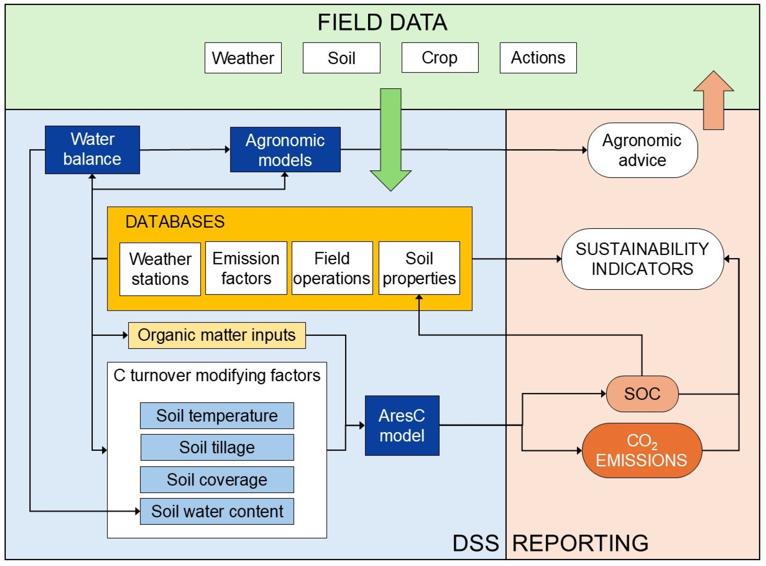
Figure 1. Data flow involved in the decision support system (DSS, light blue box), where the AresC model is integrated. The reporting outputs of the DSS are shown in light orange, while the field data used as inputs are in light green. The AresC model is then expanded in Figure 2.
Sustainability 18 07879 g001
Figure 2. Representation of carbon (C) fluxes in agricultural soils in the AresC model (blue box in Figure 1). The C pools are the light orange boxes, while the CO2 emissions are in the orange balloons. The turnover rates of the C pools are modified by factors estimated by the DSS: soil water content, soil temperature, live soil coverage and soil disturbance (see Figure 1).
Sustainability 18 07879 g002
Figure 3. Map of the case studies used for the validation of the AresC model. Critical information shown in Table 2 is included: site name, climate, type of crop, soil clay content, and duration of the experiment.
Sustainability 18 07879 g003
Figure 4. Soil C observations with standard deviation and AresC (yellow) and RothC (pink) predictions: ECS (a) and CCS (b) at Foggia site; ECS (c) and CCS (d) at Ravenna site.
Sustainability 18 07879 g004
Figure 5. Soil C observations with standard deviation and AresC (yellow) and RothC (pink) predictions: rotations 1 (a), 2 (b), 3 (c) and 4 (d) at Nyíregyháza site.
Sustainability 18 07879 g005
Figure 6. Soil C observations with standard deviation and AresC (yellow) and RothC (pink) predictions: BB (a) and AB (b) management at Lutzville; PM (c), PB (d), SM (e) and SB (f) at Valencia site.
Sustainability 18 07879 g006
Table 1. Comparison between the AresC model and other widely used SOC models: RothC, APSIM and Century.
AresCRothCAPSIMCentury
Type of modelSOC onlySOC onlyAgroecosystemAgroecosystem
Existing integration with agricultural DSSYesNoYesYes (COMET-Farm)
TimestepDailyMonthlyDailyMonthly
Soil layers115+2+
Data requirementsLowLowHighHigh
n° of pools4535
Soil water contentFAO bucket model [46]Simplified bucket modelSoilWat bucket model on different soil layers [51]Bucket models on different soil layers
Simulates water tableYesNoNoNo
Soil temperatureHeat transfer [48]Air temperatureHeat transfer [52,53]Soil surface temperature [54]
Soil tillage effectYesNoYesYes
Adapted to semi-arid conditionsYesNoYesYes
Table 2. Description of the datasets used for the case studies simulations.
SiteCoordinatesCropTreatmentsAnnual Rainfall (mm)Mean T (°C)Aridity IndexClimateUSDA Soil Texture WRB Soil Taxonomy and PropertiesYears of Experiment/Replicates n° Obs. n°/Soil Depth (cm)Ref.
Foggia, Italy41°29′27″ N, 15°30′14″ EArable crops:
Barley, wheat, sunflower in CCS, with additional lentil and cover crops in ECS
Efficient Cropping System (ECS) with cover crops, legumes and DSS use and Conventional Cropping System (CCS)55416.90.42Cold semi-aridSilty clay loamVertisol
Clay 38%
OC 2%
BD 1.1 g cm−3
8/47/
0–30
[55,56,57]
Ravenna, Italy44°29′15″ N, 12°10′44″ EArable crops:
Pea, wheat, tomato, wheat, soy in ECS, or corn, wheat, tomato, wheat in CCS
Efficient Cropping System (ECS) with cover crops, legumes and DSS use and Conventional Cropping System (CCS)65914.30.71Humid sub-tropicalSilty clay loamCambisol
Clay 29%
OC 1.4%
BD 1.1 g cm−3
8/37/
0–30
[55,56,57]
Nyíregyháza, Hungary47°58′35″ N, 21°41′50″ EArable crops:
Triticale, oat, maize and 4 cover crops
4 rotations (R1, R2, R3, R4) with unfertilized control, fertilized control, and green manures56211.90.70ContinentalSandArenosols
Clay 10%
OC 0.85%
BD 1.4 g cm−3
4/67, 6 **/
0–30
[58,59]
Lutzville, South Africa31°34′60″ S, 18°52′0″ EOrchard:
Vineyard with 8 cover crop species and control with weeds in the interrow
Full surface chemical control before bud break (BB), full surface chemical control at the end of November (AB)13918.10.09Semi-arid MediterraneanSandCambisol
Clay 0.01%
OC 0.13%
BD 1.3 g cm−3
10/73/
0–30
[60,61,62]
Valencia (Paiporta), Spain39°25′2″ N, 0°25′4″ WOrchard:
Citrus
Inter-row with bare soil (PB) or inter-row with straw mulch (PM)100418.90.50Semi-arid hot summer MediterraneanClay loamCambisol
Clay 36%
OC 0.83%
BD 1.6 g cm−3
3/111/
0–20
[63,64]
Valencia (Sueca), Spain39°12′36″ N, 0°18′23″ WOrchard:
Citrus
Inter-row with bare soil (SB) or inter-row with straw mulch (SM)100418.90.50Semi-arid hot summer MediterraneanSilty clay loamFluvisol
Clay 32%
OC 1.13%
BD 1.4 g cm−3
3/111/
0–20
[63,64]
** Nyíregyháza dataset include 7 soil samplings per treatment, except for R4 which include 6.
Table 3. Values of RMSE (%), EF, E (%) and MD (tC ha−1) for every treatment in the sites with arable crops. Values outside the brackets refer to the AresC model simulations, while values in the brackets refer to the RothC model simulations.
SiteTreatmentRMSEEFBias (E)Bias (MD)
FoggiaAll site6.6 (9.0)0.1 (−0.7)2.7 (5.1)
ECS3.2 (4.7)
CCS6.2 (8.3)
RavennaAll site10.0 (13.4)0.3 (−0.3)1.5 (3.3)
ECS5.0 (7.5)
CCS11.0 (13.1)
NyíregyházaAll site12.9 (13.2)0.6 (0.6)1.5 (3)
R16.9 (6.4)
R210.3 (10.5)
R39.6 (10.4)
R412.2 (13.0)
Table 4. Values of RMSE (%), EF, E (%) and MD (tC ha−1) for every treatment in the orchard sites. Values outside the brackets refer to the AresC model simulations, while values in the brackets refer to the RothC model simulations.
SiteTreatmentRMSEEFBias (E)Bias (MD)
LutzvilleAll sites26.0 (30.8)0.2 (−0.1)6.3 (14.7)
AB10.1 (19.9)
BB3.5 (10.0)
Grazing vetch22.8 (29.4)
Overberg oats10.8 (17.6)
Parabinga medic10.3 (15.2)
Paraggio medic5.8 (9.4)
Pink Seradella4.7 (12.7)
Rye9.3 (11.0)
Saia oats6.4 (6.1)
ValenciaAll site11.0 (13.7)2 × 10⁻² (−0.5)**−1.2 (2.5 1)
PM15.4 (18.0)
PB9.9 (15.6)
SM10.4 (8.6)
SB7.9 (13.6)
1 Significant bias; ** Relative error not determined for lack of replications.
Table 5. Values of E (%) and MD (tC ha−1), NMSE and rs for the sites grouped as orchards, arable crops and all sites. Values outside the brackets refer to the AresC model simulations, while values in the brackets refer to the RothC model simulations.
Site GroupBias (E)Bias (MD)NMSE (10−2)rs, Spearman
All sites2.9 (7.9)0.2 (1.2)1.3 (1.6)0.9990 (0.9988)
Orchard sites**−0.5 (1.8)2.2 (2.1)0.9991 (0.9986)
Arable crop sites1.9 (3.8)0.4 (1.0)1.2 (1.5)0.9982 (0.9978)
** Relative error not determined for lack of replications.
Disclaimer/Publisher’s Note: The statements, opinions and data contained in all publications are solely those of the individual author(s) and contributor(s) and not of MDPI and/or the editor(s). MDPI and/or the editor(s) disclaim responsibility for any injury to people or property resulting from any ideas, methods, instructions or products referred to in the content.