1. Introduction
As a critical node in the global supply chain, the operational efficiency of the road network in a port collection and distribution system impacts the competitiveness of the port and the sustainable development of road traffic [
1]. With the continuous growth of international trade volume, port motorways frequently experience severe congestion, leading to increased turnaround time for container trucks, higher carbon emissions, and even conflicts between port operations and urban communities [
2]. Therefore, achieving accurate and real-time traffic state information for port motorways is not only a technical necessity for smart ports but also a key enabler of sustainable intelligent transportation management. It can help reduce unnecessary truck waiting and detour, thereby lowering fuel consumption and emissions, and ultimately supporting more sustainable port traffic operations.
Due to the high costs associated sensor deployment and maintenance, it is infeasible to obtain traffic state parameters with high spatial resolution across the entire road network through detection alone. Traffic state estimation (TSE) addresses this limitation by inferring unknown traffic parameters from partially observed data [
3], thereby provides data support for network-wide traffic control and management [
4]. The effectiveness of TSE, however, is inherently constrained by the quality and distribution of the deployed sensors. This has motivated extensive research on the traffic sensor location problem (TSLP), which seeks to optimize sensor placement to maximize information gain under limited budgets. The joint consideration of sensor deployment and state estimation offers a promising pathway toward achieving accurate and cost-effective global traffic state monitoring across the entire network [
5,
6]. Existing TSE methods primarily focus on general motorways and pay attention to road traffic data itself [
7,
8]. Due to the specific characters of port motorways, corresponding TSE methods can be further developed, considering upstream port events, such as vessel arrival information.
Vessel arrivals are the fundamental drivers of demand in port collection and distribution systems. A large number of containers need to be transported by trucks in the days before and after the vessel arrives at the port. If vessel arrival information could be integrated into TSE methods, it would enable anticipation of potential traffic pressure, thereby improving estimation accuracy. However, trucks arrive in a few days before the Container Yard (CY) closing time, which means a significant spatial and temporal mismatch exists between vessel arrival information and road traffic data. Therefore, effectively fusing such heterogeneous and asynchronous multi-source data presents a major challenge for current research.
Therefore, the overall goal of this study is to develop a TSE method that can not only complete the unobserved traffic state information, but also integrate the vessel influence. To address this problem, this paper proposes a novel TSE method for port motorways named Heterogeneous Graph Convolutional Network with Vessel-aware Attention (HGCN-VA) based on graph neural networks (GNNs), aiming to integrate vessel arrival information as prior knowledge into traffic state modeling. Specifically, we first introduce an influence weight learning module based on an attention mechanism to adaptively model the spatiotemporal intensity of vessel events’ impact on the traffic state of the surrounding road network, thereby resolving the information asynchrony issue. Subsequently, we construct a heterogeneous graph convolutional network (HGCN) containing both road nodes and port nodes, where port nodes characterize features of vessel arrival events. Finally, this is combined with a multi-layer perceptron (MLP) to capture the temporal evolution patterns of traffic flow.
In summary, our main technical contributions are as follows:
- (1)
We propose a GNN-based approach for port motorway TSE. This approach integrates the vessel arrival information, providing a more event-informed modeling perspective for port collection and distribution systems, different from the traditional TSE that relies solely on traffic data.
- (2)
We design a heterogeneous diffusion graph convolutional network that uniformly models port models and road nodes, and learns the dynamic influence weights of vessel events using an attention mechanism, effectively addressing the spatiotemporal mismatch problem.
- (3)
Evaluations on a simulation-based port dataset demonstrate that our model benefits from vessel information, which provides better performance than other baselines.
The remainder of this article is organized as follows.
Section 2 briefly reviews the related works.
Section 3 presents the methodology.
Section 4 discusses the experiment results of the proposed model.
Section 5 concludes the paper and outlines potential future directions.
2. Literature Review
2.1. GNN-Based Traffic Kriging and State Estimation
Kriging is a geostatistical interpolation technique widely used for spatial prediction, while TSE refers to the process of inferring unobserved traffic variables from limited measurements. Both approaches aim to estimate traffic conditions at locations without direct observations. Ordinary Kriging (OKriging) [
9], the most widely used Kriging method, estimates unobserved values by modeling spatial dependence through covariance and variogram functions. These functions quantify how correlation decays with spatial distance.
In recent years, GNN-based inductive methods have emerged to conduct spatiotemporal Kriging. Appleby et al. [
10] proposed a Kriging model based on a graph convolutional network (GCN) to conduct estimation using neighbor observations. Wu et al. [
11] further designed a diffusion graph convolutional network (DGCN) model by means of training procedure for inductivity. Liang et al. [
12] developed a spatial–temporal-aware GNN model to handle random, segment and blockout missing tasks.
These methods are developed based on predefined adjacency matrices. However, spatial dependencies between nodes are complex, influenced not only by topological structures but also by potential implicit correlations, which predefined graph structures may fail to adequately capture. To address this issue, dynamic graph neural network techniques have emerged, enabling the generation and analysis of time-evolving graph structures. Nie et al. [
13] proposed a speed pattern adaptive graph neural network that leverages observed node speed measurements from floating car data to estimate traffic flow at unobserved locations. Pan et al. [
14] introduced a graph transformer model that enhances the model’s receptive field to mitigate the challenge of edge information aggregation, thereby effectively capturing spatiotemporal features. Wei et al. [
15] proposed an inductive framework that fuses learnable node embeddings for dynamic graphs with pre-defined static graph structures, while also adding an auxiliary objective to compensate for information loss due to random subgraph sampling. However, since the embedding learning relies on loss functions that require full node attributes, the resulting dynamic features cannot be easily transferred to unobserved nodes without those attributes. To tackle this problem, Wu et al. [
16] introduced a different strategy that employs multiple aggregation functions in spatial message passing, which captures richer spatial dependencies and ultimately boosts both generalization and estimation performance.
Most of the above studies rely solely on data collected from detectors. Given the limited capacity of single data sources, some research has begun exploring the integration of multi-source data into traffic state estimation models to improve estimation accuracy by fusing richer information. Yao et al. [
17] constructed a spatial interaction graph convolutional network using the location attributes and flow attributes of geographic units to impute missing origin–destination (OD) flow data. Zheng at al. [
18] incorporated multi-source data, including points of interest and OD information, to enhance model accuracy.
In addition to real-time state estimation, traffic prediction constitutes another important research direction in intelligent transportation systems. Leveraging the capability of graph neural networks to model complex spatial dependencies, they have also become a significant technical approach in traffic prediction, with representative models including Spatial–Temporal Graph Convolutional Networks (STGCNs) [
19], Diffusion Convolutional Recurrent Neural Networks (DCRNNs) [
20], and Attention-Based Spatial–Temporal Graph Convolutional Networks (ASTGCNs) [
21]. However, these methods typically assume the availability of observations at all locations and cannot be directly applied to unobserved locations lacking historical data. Therefore, many studies have further investigated traffic prediction for unobserved locations while accounting for real-time spatial interpolation. Roth and Liebig [
22] proposed an enhanced graph attention mechanism that adaptively assigns different weights to neighboring nodes based on node embeddings to model spatiotemporal correlations for global prediction. Mei et al. [
23] developed an uncertainty-aware framework based on a diffusion graph convolutional model to predict traffic states at locations without historical data, generating probabilistic predictions with uncertainty quantification. Zhou et al. [
24] introduced an inductive spatiotemporal graph model that incorporates a mixture of graph experts with a sparse gating mechanism to dynamically and efficiently capture heterogeneous spatial dependencies for global traffic prediction. Zhou et al. [
25] proposed the Directed Graph Autoencoder (DGAE) that tackles TSE under sparse sensors by introducing a Dirichlet energy-based feature propagation for directed graphs (DEFP4D), eliminating zero-filling bias while separately handling congested and free-flow patterns. Zhao et al. [
26] proposed a structure-inductive meta-learning scheme (SIML) to learn a mask-agnostic initialization via volatility-guided task curriculum, structure consistency regularization, and structure-aware replay.
However, the applicability of these GNN-based Kriging methods to port motorways is inherently limited. Most of these methods assume homogeneous node types and predefined road network topologies, treating all nodes as identical traffic sensors. Their graph structures are either fixed or updated purely based on traffic flow dynamics. These designs overlook cross-domain interactions from external entities such as port terminals, whose operational events are primary drivers of downstream truck demand.
2.2. Traffic Research on Roads Surrounding Ports
Much research focuses on roads surrounding ports due to their special traffic characteristics. About the bidirectional influence between road traffic systems and ports, Pope et al. [
27] identified that fluctuations in port cargo throughput and the carrying capacity of surrounding arterial roads significantly affect port operational efficiency, with port activities also inducing long-distance congestion effects on adjacent areas. Yang et al. [
28] developed a traffic demand model for container trucks based on ship operation schedules and truck arrival patterns, further incorporating external corrective factors. Focusing on the negative impacts of port activities on urban road networks. Ziemska-Osuch and Guze [
29] conducted a case study at the Port of Gdynia, revealing that even slight increases in heavy truck flows can substantially degrade road service levels during evening peak hours, and suggested that bypass roads could enhance network connectivity to mitigate port–city conflicts. Bernacki et al. [
30] decomposed the urban port transportation system into a road subsystem directly accessing the port transfer area and a mixed road subsystem, providing long-term traffic and freight flow predictions to support system planning. Caldeira et al. [
2] developed a dynamic road–port passage model and validated its applicability for evaluating port–city relationships at the Port of Santos. Bernacki et al. [
31] further quantified the sustainability benefits of road infrastructure improvements in local urban port transportation systems, demonstrating that such investments reduce congestion and increase truck speeds. Zhang et al. [
32] employed the traditional four-step method to plan a comprehensive transportation hub in the Mississippi port area based on cargo flow survey data.
In conclusion, the roads around the port area have their unique traffic characteristics, and these characteristics are closely interrelated with the port. Although there is still a lack of sufficient research specifically on the traffic state estimation of the port’s collection and distribution road network at present, many studies have focused on the prediction of road truck traffic. For instance, Xie and Huang [
33] established Gaussian processes and
-SVM (
-support vector machine based on the Sigmoid kernel function) to predict the daily arrival volume of pick-up and delivery trucks at container terminals. Kourounioti et al. [
34] used a fully connected neural network (FCNN) combined with auxiliary factors such as container and yard information to improve the fitting performance of the port container dwell time distribution and analyzed the influence of various forms of information. Gao et al. [
35] utilized the Long Short-Term Memory (LSTM) model to predict the daily number of containers entering the yard. Luo et al. [
36], based on the theory of cargo traffic flow induced by port vessel operations, constructed a short-term truck flow prediction model based on the remaining distribution weight of vessel cargo. Nadi et al. [
37] used operational logistics information among terminal operators, carriers and shippers, and adopted a feedforward neural network to predict the short-term arrival volume of trucks at major container terminals in seaports. Li et al. [
38] for the first time incorporated factors such as vessel-related information, working days of arrival and weather conditions into the long-term sequence of truck arrivals at the port, and applied a deep learning model to predict the daily arrival volume of trucks.
While these studies recognize the importance of interactions between port activities and road traffic, they predominantly concentrate on aggregate traffic demand forecasting rather than on estimating real-time, segment-level traffic states, which are more helpful for network-wide traffic control, ramp metering, and dynamic route guidance. Moreover, these studies rarely employ spatial interpolation to reconstruct unobserved locations from sparse detector data; they either rely on historical averages or require full coverage of observations, which is infeasible given the high cost of sensor deployment on extensive port motorway networks. Consequently, the critical link between vessel-induced demand generation and the resulting spatiotemporal evolution of road traffic states remains underexplored in the domain of state estimation, leaving a clear gap between port activity awareness and operational traffic management.
3. Methodology
In this section, we formally present the mathematical formulation of the traffic state estimation (TSE) problem. First, we outline the framework of the proposed model to illustrate how the estimation problem is solved through the organization and collaboration of the modular components. Subsequently, we detail three core modules designed to handle different types of correlation: feature generation, spatial, and temporal modules.
3.1. Problem Formulation
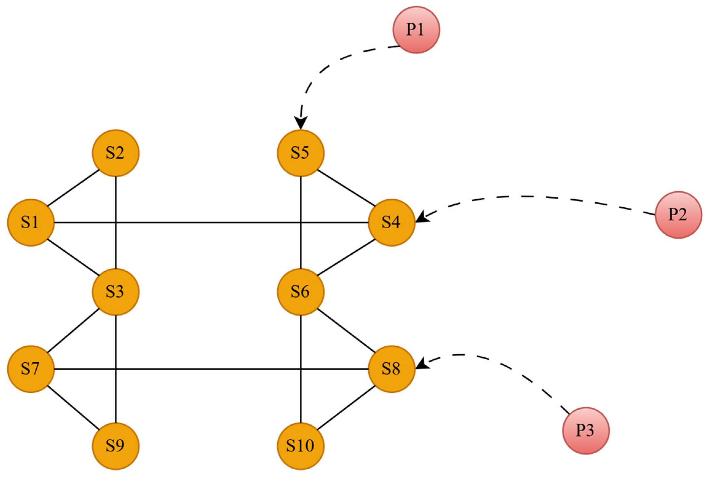
In our study, TSE is defined as the task of inferring continuous traffic variables over a road network from sparse observations. We formulate TSE as a spatial Kriging problem, which is a geostatistical interpolation technique. The topological constraints that regulate traffic state propagation make graph representations a natural choice for modeling transportation networks. Accordingly, as shown in
Figure 1, we represent the whole network as a directed heterogeneous graph
, with
being the node set and
the edge set. In this paper,
comprises two types of nodes, namely road nodes
and port nodes
. Let the set of sensor nodes be
and the set of port nodes be
, where
and
denote the numbers of sensors and ports, respectively. Correspondingly,
consists of two types of connections: edges between sensor nodes and edges between sensor nodes and port nodes. We define
as the weighted adjacency matrix whose elements storing the corresponding edge weights.
In the literature, a commonly used distance-based adjacency matrix
is computed as [
20]:
where
is the travel distance between two nodes which can be road sensors or port,
is a scaling parameter which can be selected as the standard deviation of distance, and
is the threshold. As shown in Equation (1),
is asymmetric because the traffic graph is directed.
Based on Equation (1), we define four types of adjacency matrices:
Sensor-sensor upstream adjacency matrix : each element indicates that sensor node is upstream of sensor node .
Sensor-sensor downstream adjacency matrix : each element indicates that sensor node is downstream of sensor node .
Port-sensor adjacency matrix : each element indicates that port node points to sensor node . It is computed as the travel distance between the two nodes via the road network, weighted by a Gaussian kernel. This captures the influence of port activities (e.g., truck departures from the port) propagating to downstream road sensors.
Sensor-port adjacency matrix , where each element indicates that sensor node points to port node . It is computed as the travel distance between the two nodes via the road network, weighted by a Gaussian kernel. This captures the influence of traffic conditions on road segments toward the port (e.g., trucks approaching the port).
Based on this heterogeneous graph, we formulate the TSE problem as follows. Road and port measurements operating on the graph can be recorded as graph signals. We define the following notations:
Road sensor features : is the number of sensor nodes and is the number of time intervals. Each element represents the traffic speed at sensor during time interval .
Port features : is the number of port nodes and is the number of days. Each element represents the vessel arrival count at port on day . The port feature matrix is defined over a ( + 30)-day window (15 days before and after the simulation days), where each entry represents the daily vessel arrival count for a given port.
The objective of TSE is to reconstruct the current traffic speeds at all sensor nodes given the incomplete observations and the heterogeneous graph structure. Formally, our task is to achieve a mapping function
parameterized by
that estimates the target traffic state
from the input
and the graph
as follows:
At the operational stage, the trained model consumes real-time measurements from arbitrary sensors and reconstructs the full-scale traffic states over the whole road network.
3.2. Framework of HGCN-VA
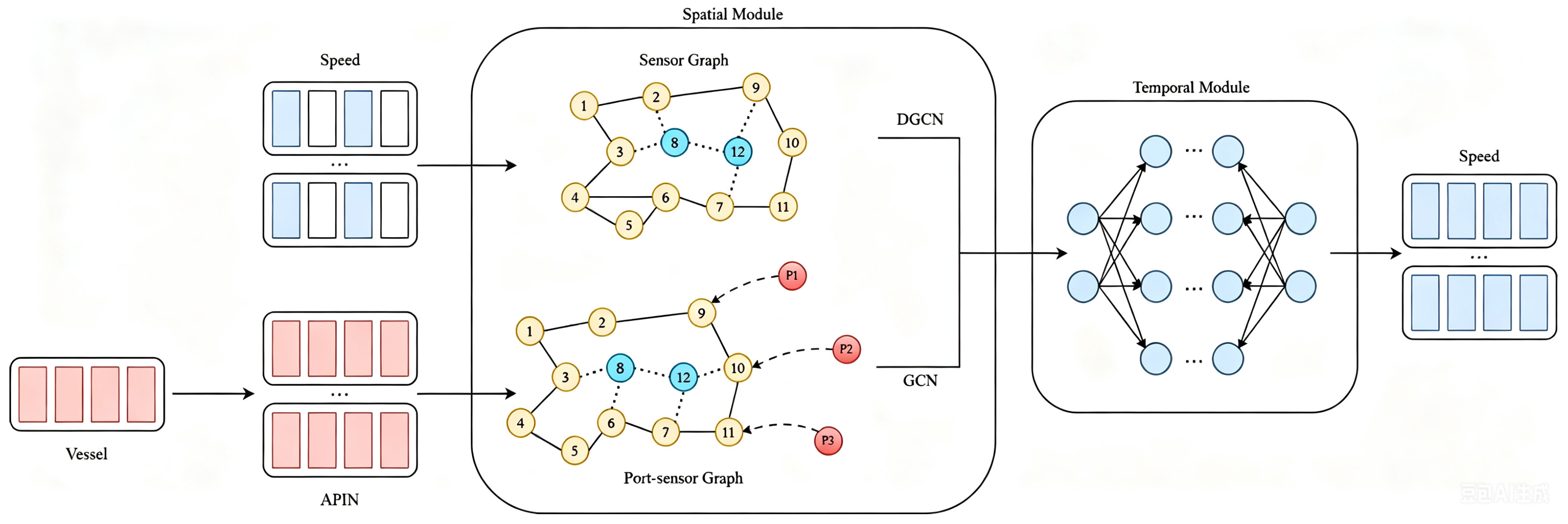
The overall framework of HGCN-VA is presented in
Figure 2, which consists of three core components: the influence weight learning module, the DGCN-based spatial module, and MLP-based temporal module. In the framework, port data need to be put into the influence factor learning module firstly in order to align with road traffic data. Then, incomplete traffic data and influence factor are put into the model, it can handle spatial and temporal dependencies through corresponding modules. Finally, we can get the reconstructed traffic data.
3.3. Influence Weight Learning Module
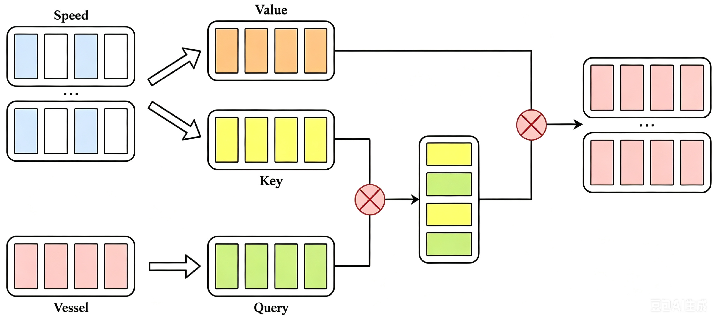
The heterogeneity between traffic flow data and vessel data makes direct alignment challenging. Simply concatenating vessel features with traffic speed observations fails to capture the dynamic influence of port activities on road traffic. To address this issue, we propose an Adaptive Port Influence Network (APIN) module based on the attention mechanism. APIN dynamically estimates the time-varying impact of each port on the surrounding road network, using the current speed state as contextual information, as shown in
Figure 3.
Specifically, the module takes as input the road speed tensor and the port feature matrix, and outputs a weight matrix that represents the influence intensity of each port at each time step. The computation proceeds as follows.
Firstly, we aggregate the observable road speed data along the spatial dimension to obtain a global speed pattern of the road network. The average speed at time
is computed as Equation (3):
Next, we project the aggregated speed and the port features into a common latent space via separate linear transformations, as shown in Equation (4):
where
and
are learnable parameters, and
is a nonlinear activation function (e.g., ReLU or sigmoid).
Then, we utilize attention mechanism to calculate the influence weights of ports. Here, the query is derived from the speed context, while the key is derived from the port features, as shown in Equation (5):
The attention score between each port and each time step is then computed as Equation (6) [
39]:
where
is a scaling factor to stabilize gradients.
The result matrix quantifies the influence of each port at each time step, conditioned on the current road speed pattern. This impact factor is then used to modulate the integration of port information into the downstream graph convolution layers.
In both training and inference, the average speed in Equation (3) is computed only over the set of currently observed sensor nodes. During training, this set corresponds to the unmasked nodes in the sampled subgraph; during inference, it corresponds to the actual available sensors in the deployment scenario.
3.4. HGCN-Based Spatial Module
To capture the complex bidirectional spatial dependencies within the port motorways, we propose a hierarchical spatial module based on homogeneous and heterogeneous DGCNs. As illustrated in the framework, this module consists of two stages: the first several layers employ heterogeneous DGCNs to model information propagation across different node types, while the subsequent layers employ standard DGCNs to capture the pure traffic flow dynamics within the road network. The hierarchical design allows the model to first integrate the exogenous influence of vessel events into the road network representation, and then refine the spatial dependencies among road segments using the learned contextualized features.
For any node on a sensor graph, both inflows and outflows decide its instant traffic state. Therefore, bidirectional traffic networks encourage a model that can deal with asymmetric adjacency matrix. We adopt DGCN model as the propagation layer to handle this directed graph. DGCN treats forward edges and backward edges separately by two adjacency matrices [
11]. We denote the diffusion steps as
, and the diffusion graph convolution layer can be written as
where
and
are the forward and backward transition matrix at the
th diffusion step,
is the total steps of diffusion, and
are learnable parameters of DGCN layer. The bidirectional transition matrices can be obtained from the adjacency matrix of sensor graphs as follows:
and are in fact the row-wise normalization of and , in order to sum the weights to one. This diffusion convolution operator can take into account the influence of inflows and out flows simultaneously.
The standard DGCN assumes homogeneous node types and uniform edge semantics, which is sufficient for our task where port nodes and sensor nodes have distinct feature spaces and interaction patterns. To address this, we propose a heterogeneous graph convolutional network (HGCN) model that explicitly accounts for node heterogeneity. The basic form is as follows:
In Equation (9), the HGCN performs forward and backward diffusion to capture spatial dependencies, while conducting single graph convolution to extract port correlations. In this way, we inject the port information into HGCN-VA adaptively and can capture multiresolution dependencies in a unified module. Graph convolution is performed on each time slot, which can be parallelized across time.
The overall spatial module stacks layers of the HGCN followed by layers of the standard DGCN. The initial layers focus on integrating cross-domain information from port events, learning the spatial influence patterns. The later layers then refine the representations by focusing on the traffic dynamics within the road network itself. By switching to standard convolution after the heterogeneous layers, we avoid the overhead of maintaining separate weight matrices for edge types in deeper layers, where the need for explicit heterogeneity diminishes.
We first customize the HGCN layer as follows:
where
is the output spatial features of the
th HGCN layer. By stacking several HGCN layers, the model can capture multi-hop spatial correlations on the graph and the features of each node contain information from neighbor nodes and port nodes.
The middle variable
is computed as follows:
After the initial layers of heterogeneous diffusion convolution, the port node representations have been effectively propagated into the road network nodes, enriching the sensor features with vessel event context. In subsequent layers, we transition to a standard diffusion graph convolution that operates exclusively on the sensor node subgraph, focusing on modeling the intrinsic traffic flow dynamics among road segments.
3.5. Temporal Module
After capturing spatial dependencies, we further extract the correlations in the time dimension. Some classical temporal models are applied to extract features of a sequence such as time series. It has been proven that MLP can also achieve satisfying performance in capturing temporal correlations, which is simpler and more efficient [
40,
41,
42]. The specific formulation is shown as follows:
For our real-time Kriging task, the recovery window is relatively short. Therefore, we simply assume that all time points in the recovery window are correlated with each other.
3.6. Training and Loss Function
As mentioned in
Section 3.1, our task is to reconstruct the missing sensor data. We set the loss function to the overall reconstruction error across all nodes, seen and unseen, to promote a message-passing process that is not biased toward any subset, expressed as Equation (14):
where
denotes the estimated value and
is the true value.
To learn generalized graph convolution and adapt to novel network structures, we employ a training strategy based on stochastic subgraph sampling. Algorithm 1 provides the pseudo code of training strategy. In this strategy, each training iteration randomly samples a subgraph from the full graph constructed by observable sensors. Within the sampled subgraph, a subset of sensor nodes is randomly masked to simulate missing observations. The model is then trained to reconstruct the masked node features from the remaining observed nodes and the subgraph structure. By repeatedly exposing the model to diverse subgraphs and different masking patterns, the spatial dependencies are learned in a way that does not rely on fixed node identities. Consequently, the trained model can achieve inductivity, which means it can be directly applied to unseen nodes as long as their connectivity and neighbor observations are available.
| Algorithm 1 HGCN-VA Training Procedure |
Input: Training speed data: , Port feature matrix: Adjacency matrices: Time window length , Hidden dimension , Diffusion steps , Batch size , Number of batches , Masked nodes per sample , Max iterations Output: Trained model Initialize the model as for iteration to do for batch to do Generate batch indices: Initialize for sample to do Extract time sequences: Generate node mask: end for Prepare masked input: Forward pass Compute loss computed by Equation (14) Backward pass & update Compute w.r.t parameters Update parameters with Adam end for end for Return
|
4. Experiments
In this section, we introduce the experiment environment, also evaluating the proposed model with an extensive number of experimentations.
4.1. Simulation Dataset
In this section, we validate the proposed TSE method on a traffic simulation example generated in Python. We conduct this simulation using a modified version of the Uxsim mesoscopic traffic simulation [
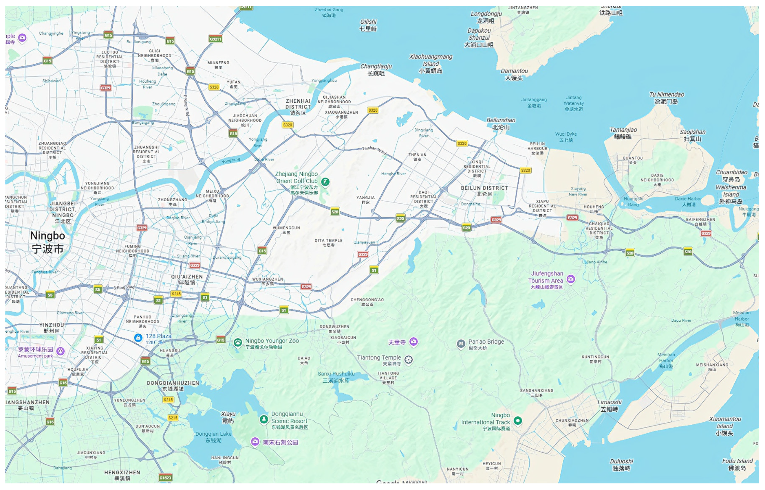
43], extended to support heterogeneous vehicle types (passenger cars and container trucks) and output data for different vehicle types. The simulated network is located in Ningbo, China, adjacent to three ports, namely Chuanshan, Beilun, and Meishan, as shown in
Figure 4. The network covers 330 km of bidirectional motorways with 658 virtual detectors placed every 500 m. the simulation time is 24 h with a time step of 5 s.
Passenger car demand follows a diurnal pattern with peak factors of 1.2–1.5 during morning (07:00–09:00) and evening (16:00–19:00) peaks, and a factor of 0.05–0.15 at night (00:00–06:00). Baseline flows are 720–1080 veh/h/ln on mainlines and 288–540 veh/h/ln on ramps.
Vessel arrivals are generated for three ports with daily frequencies of 13–15 (Chuanshan), 8–10 (Beilun), and 10–12 (Meishan), which are approximately in line with real conditions. Two vessel types are considered, large (8000–20,000 TEU, 40% of arrivals) generating 2300–5800 truck trips, and medium (2000–5000 TEU, 60%) generating 300–1450 truck trips.
The temporal pattern of truck demand differs fundamentally between export and import operations. For export containers, truck arrivals concentrate in the days prior to the vessel’s closing time, with an increasing intensity as the deadline approaches—a pattern known as the “deadline effect.” For import containers, trucks do not arrive immediately upon vessel arrival; rather, they begin arriving after customs clearance is completed and the container becomes available for pickup, typically 2–7 days after vessel arrival, and may continue over the subsequent free period (7–14 days). The total influence of a vessel event on port motorway traffic can thus span 10–20 days.
To incorporate these realistic patterns while maintaining computational tractability, the influence of vessel events on truck demand is modeled using a multi-window stepped function. For export containers, the truck generation multiplier β is set to 0.1 for the period 14–7 days before vessel arrival, 0.3 for 7–2 days before, and 0.6 for the final 48 h. For import containers, β is set to 0.15 for days 2–5 after arrival, 0.08 for days 5–10, and 0.03 for days 10–14. This stepped approximation captures the key temporal dynamics without introducing the complexity of continuous decay functions.
Detailed simulation settings—including node and link models, heterogeneous fundamental diagram derivations, route choice logic, and a qualitative plausibility check—are provided in
Appendix A.
4.2. Baselines
To comprehensively evaluate the performance of our proposed method, we compare it against several representative baseline methods from different types of techniques, which are widely adopted benchmarks in spatiotemporal Kriging tasks, including classical geostatistical interpolation OKriging, the distance-based nonparametric method k nearest neighboring (KNN), the classical GNN model graph convolutional network (GCN), inductive graph neural network Kriging (IGNNK), and tensor completion approaches such as Laplacian enhanced low-rank tensor completion (LETC). This multi-family selection enables us to assess the added value of our vessel-aware heterogeneous design relative to both traditional and modern learning-based baselines. The details are as follows:
OKriging: Ordinary Kriging interpolates the values at unmeasured locations by modeling spatial dependence through a semi variogram, assuming an unknown but constant mean. It serves as a baseline for traditional spatial interpolation without exploiting network topology.
KNN: KNN is a nonparametric spatial interpolation method that estimates unobserved traffic states as the arithmetic mean of the observed values from the k nearest neighboring sensors. It represents a simple distance-weighted approach commonly used in transportation.
GCN: GCN is a seminal graph neural network that performs convolution operations directly on graph-structured data. It learns node representations by iteratively aggregating and transforming feature information from local neighborhood of each node [
44]. GCN exploits the natural graph topology of road networks to capture spatial dependencies among sensors.
IGNNK: IGNNK is a representative inductive GNN designed for spatiotemporal Kriging tasks. By propagating information along both upstream and downstream directions, it captures the asymmetric spatial dependencies inherent in traffic flow, while its inductive design allows direct application to unseen sensor locations [
11].
LETC: LETC addresses the traffic speed imputation problem through tensor completion, where spatial correlations are regularized by a Laplacian penalty and temporal continuity is preserved via low-rank tensor approximation. It provides a complementary baseline that explicit message passing, offering a different perspective from graph neural networks [
45].
By comparing with OKriging and KNN, we evaluate the improvement brought by deep learning and graph-aware modelling. The inclusion of GCN and IGNNK allows us to benchmark against both basic and advanced GNN architectures, while LETC tests the effectiveness of our method against a powerful non-GNN alternative that also handles missing data. For fair comparison, we use the same training, validation and test splits and the same set of observed sensors as our model.
4.3. Settings
The experimental configuration is set as follows. All nodes are randomly split into two groups: monitored sensors and unmonitored points. For the baseline deep learning models, the temporal dataset is allocated into 70% for training, 10% for validation, and the remaining 20% for testing. Regarding the key hyperparameters of HGCN-VA, the number of diffusion steps is fixed to 1, while DGCN and HGCN are configured with 3 and 1 layers, respectively. The hidden dimension is set to 80, and we employ a batch size of 32 with the Adam optimizer and a fixed learning rate of 1 × 10⁻³. Initial experiments are conducted with a sensor coverage of 70%—specifically, 461 sensors are randomly chosen as observed locations for model training, 59 are held out for validation, and the remaining 138 serve as test points for evaluation.
To examine the feasibility of our approach in real-world scenarios, we record the training duration, inference latency, peak memory consumption, and computational complexity. All experiments run on a Windows 11 machine equipped with an Intel Core i5-12500H CPU and an NVIDIA GeForce RTX 3050 GPU, using Python 3.12.0 and PyTorch 2.3.0. The training phase consisted of 150 epochs and took a total of 303 s. During inference, processing a single test sample required an average of 20 milliseconds. The peak memory usage throughout the pipeline was approximately 1.5 GB.
4.4. Metrics
To quantify our model performance and compare with other baseline methods, we choose the following three metrics:
Mean Absolute Error (MAE) measures the average magnitude of absolute errors between ground truth and estimated values, defined as Equation (15):
where
and
denote the estimated value and the ground truth, respectively, and
is the total number of test samples.
Root Mean Square Error (RMSE) quantifies the square root of the mean squared error between the ground truth and the estimated values, calculated as Equation (16):
Mean Absolute Percentage Error (MAPE) is defined as the mean absolute percentage error with respect to the ground truth, as given in Equation (17):
In contrast to the training phase, the testing stage focuses exclusively on the performance at the target estimation locations, rather than encompassing all nodes within the study area. This targeted approach enables a direct and unambiguous evaluation of model effectiveness.
4.5. Imputation Performance
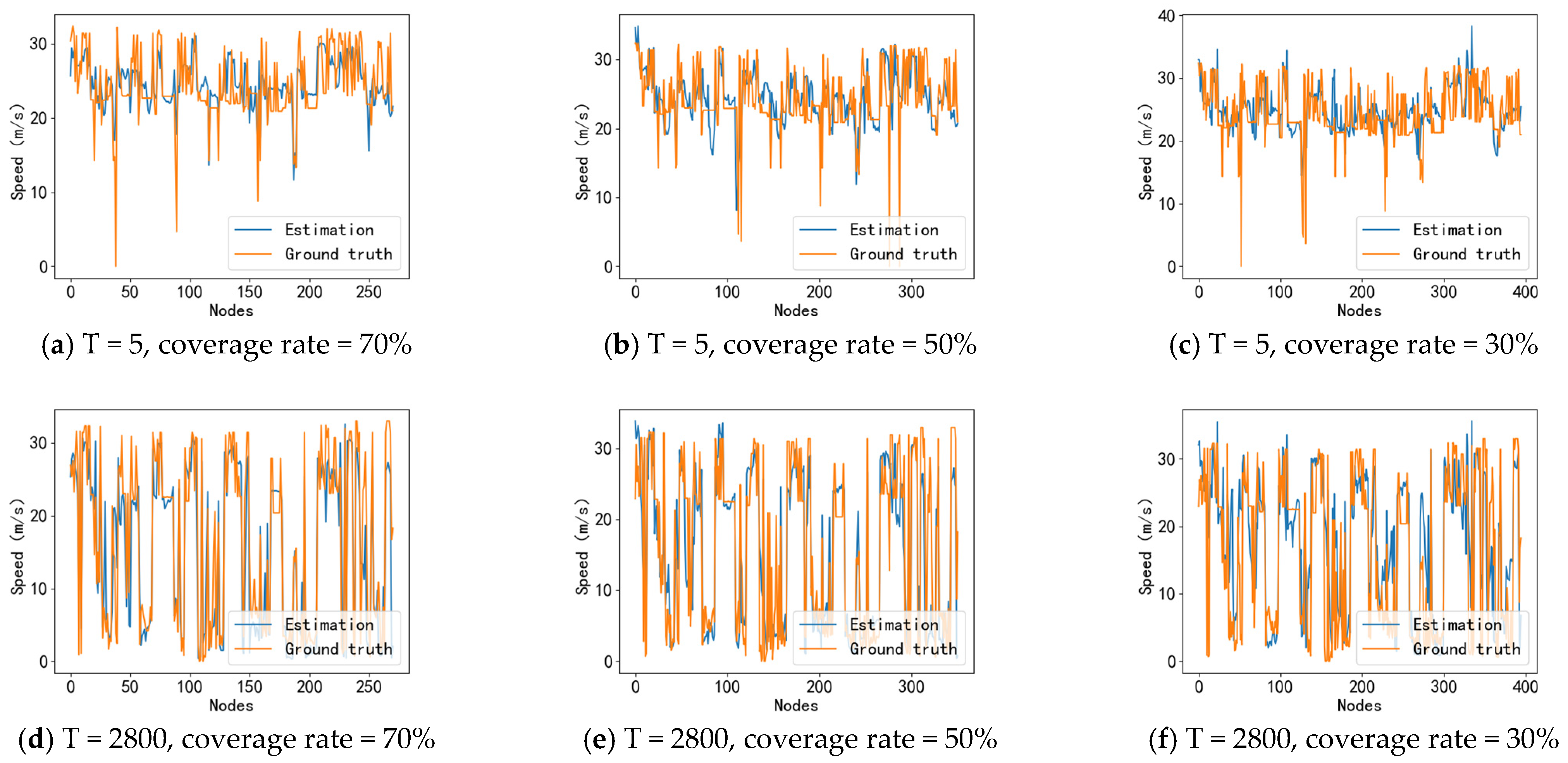
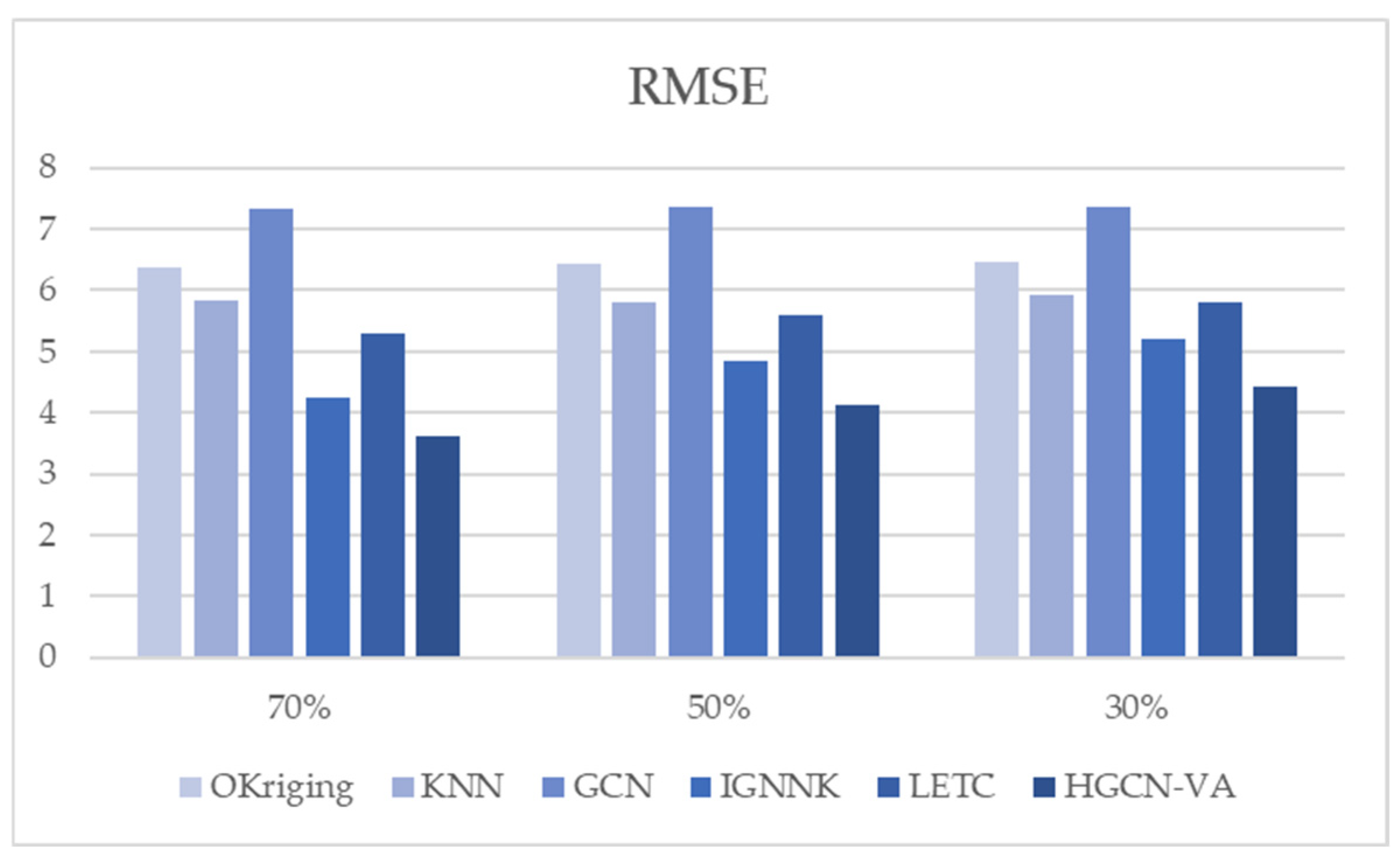
To demonstrate the superiority of our model, we compare it with baseline methods under missing-data conditions at 70%, 50%, and 30% sensor coverage. The results, summarized in
Table 1 and visualized in
Figure 5, show that HGCN-VA consistently outperforms the others;
Table 1 in particular gives a quantitative error comparison for speed estimation.
The experimental results demonstrate the strong performance of the proposed HGCN-VA model. As summarized in
Table 1, all compared methods achieve reasonably low estimation errors under the evaluated settings, with the proposed model consistently attaining the lowest error across all metrics. This indicates that HGCN-VA not only benefits from the expressive power of graph neural networks but also effectively leverages the heterogeneous graph structure and vessel-aware attention mechanism. To further illustrate the model’s estimation capability,
Figure 6 provides a detailed time series comparison between the estimated speeds and the ground-truth values at several representative locations. It can be observed that the estimates produced by HGCN-VA closely follow the ground-truth trajectories, accurately capturing both free-flow conditions and the onset, evolution, and recovery of congestion. These results confirm that the proposed approach preserves the temporal dynamics of traffic states while achieving high spatial interpolation accuracy.
To further explore the function of HGCN-VA, we compare the HGCN-VA with the ablated model in the two special scenarios, points near the ports and far away from the ports. The results are shown in
Table 2. Our proposed model performs better at points near ports, while the ablated model performs better at points far away from ports.
4.6. Ablation Study
To quantify the contributions of the port-related module in the proposed model, we conduct an ablation study at 70% coverage rate by removing the specific module.
HGCN-VA w/o MLP: We remove the MLP-based temporal module.
HGCN-VA w/o DGCN: We replace HGCN and DGCN with symmetric spectral convolution.
HGCN-VA w/o HGCN: We replace HGCN with a standard DGCN model.
HGCN-VA w/o APIN: We replace APIN with directly concentrating port features.
As reported in
Table 3, the full HGCN-VA outperforms all its ablated counterparts, confirming that each module contributes meaningfully. The removal of either spatial or temporal components considerably inflates estimation error, indicating that speed patterns rely on both spatial and temporal processes. Meanwhile, dropping the HGCN layer impairs accuracy, which points to the influence of port zones on roadway conditions, and omitting APIN uncovers the time-varying connections between ports and roads. Overall, these results reinforce the necessity of explicit port feature encoding.
4.7. Model Analysis
To investigate the impact intensity of ports on estimation accuracy, we conduct model sensitivity studies on the number of HGCN layers.
Table 4 shows the estimation results under the condition of 70% average rate. As shown in
Table 4, the model achieves optimal performance with a single heterogeneous graph convolution layer. Performance degrades progressively as the number of layers increases, suggesting diminishing returns from incorporating additional port area information. While port area features do exert a measurable influence on road traffic state characterization, their temporal and spatial relationship with road-level traffic dynamics is indirect, as evidenced by the operational characteristics of port areas. Excessive integration of such domain-specific information may therefore introduce noise and hinder model convergence during training. Consequently, this study concludes that port area information serves as a beneficial auxiliary signal for traffic state estimation, yet its contribution remains secondary and bounded. Road network topology and spatiotemporal correlations should remain the primary modeling focus; the heterogeneous graph convolution module designed for port area features functions most effectively as a complementary component, jointly enabling optimal estimation performance.
5. Conclusions
Port motorways suffer from sparse traffic detector coverage, and port activities add extra complexity, posing significant challenges to the acquisition of high-resolution spatiotemporal traffic information. The resulting data gaps pose serious obstacles to real-time operational control of port access and distribution networks. Most existing TSE methods focus on general motorways and urban roads, while few of them considering port motorways. To explore the novel TSE methods of this specific scenario, this paper introduces a novel GNN-based method named HGCN-VA which is characterized by its ability to integrate vessel arrival information into TSE.
For this purpose, we design an influence-weight learning module APIN that adaptively aligns asynchronous port features with road traffic data. We further propose a hierarchical spatial module consisting of HGCN layers to model cross-domain port–road interactions, followed by standard DGCN layers to capture intrinsic traffic propagation patterns. Extensive experiments on a simulated port motorway dataset demonstrate the effectiveness of HGCN-VA. The key findings are as follows:
- (1)
High accuracy in sparse-data scenarios: In contrast to competing approaches, HGCN-VA delivers consistently superior estimation precision under various levels of sensor sparsity, demonstrating both marked performance gains and strong resilience to missing observations. This robustness is particularly notable at low coverage rates, where traditional methods suffer from substantial performance degradation due to insufficient spatial information, whereas our model maintains reliable estimation by effectively leveraging vessel-aware prior knowledge and heterogeneous graph propagation.
- (2)
Effectiveness of port information integration: Ablation studies confirm that removing the HGCN or APIN module leads to notable performance degradation, especially in near-port areas. The proposed model achieves lower estimation errors near ports while maintaining comparable performance in far-port areas. This indicates that the vessel-aware attention mechanism successfully captures the spatiotemporal influence of port activities on surrounding road segments, and that the hierarchical spatial design, combining heterogeneous and standard diffusion convolutions, effectively balances cross-domain information integration with intrinsic traffic dynamics.
The proposed model uses existing detector data and vessel schedules to estimate network-wide traffic states in near real time. This reduces sensor deployment costs, enables proactive congestion management informed by vessel arrivals, and supports sustainable port operations by cutting truck fuel consumption and emissions. From a practical standpoint, the inductive nature of the framework further allows immediate application to newly installed sensors without retraining, offering flexibility for incremental network expansions in evolving port environments.
There are several limitations remaining. First, while initial validation is conducted using simulation data, it is essential to introduce more abundant real-world data into the evaluation process, in order to identify more realistic external factors, such as weather conditions, traffic accidents, road maintenance, and public holidays. Then, more physical law in port–road interactions need to be explored, including developing models with more physical significance, exploring vessel-to-traffic propagation delays and so forth. Integrating causal discovery or counterfactual reasoning into port motorway TSE is also a promising direction, for instance by using port closure events as natural interventions or employing structural causal models. What is more, sensor configuration should be considered together with TSE.
Author Contributions
Conceptualization, X.L., H.Y. and P.Z.; methodology, X.L., Y.W. and P.Z.; software, X.L.; validation, Z.H., M.P. and P.Z.; formal analysis, X.L. and H.Y.; investigation, X.L.; resources, P.Z.; data curation, X.L.; writing—original draft preparation, X.L.; writing—review and editing, Z.H. and H.Y.; visualization, X.L.; supervision, Y.W., M.P. and P.Z.; project administration, P.Z.; funding acquisition, P.Z. All authors have read and agreed to the published version of the manuscript.
Funding
The work was supported in part by the National Natural Science Foundation of China (52272334), the Key R&D Program of Zhejiang Province (2024C01180), EC H2020 Project (690713), the National Key Research and Development Program of China (2017YFE0194700), and the Fundamental Research Funds for the Provincial Universities of Zhejiang (SJLY2025006).
Institutional Review Board Statement
Not applicable.
Informed Consent Statement
Not applicable.
Data Availability Statement
The data are available from the corresponding author on reasonable request.
Acknowledgments
We would like to thank the National ‘111’ Centre on the Safety and Intelligent Operation of Sea Bridges (D21013) and the Zhejiang 2011 Collaborative Innovation Center for Port Economy for the support in providing academic and technical resources. The authors would like to thank the K.C. Wong Magna Fund at Ningbo University for their sponsorship.
Conflicts of Interest
The authors declare no conflicts of interest.
Appendix A. Simulation Platform for Port Motorway Network
The appendix provides a detailed description of the simulation platform used to generate the dataset for this study. The platform is built upon the UXSIM mesoscopic traffic simulator [
43] and is extended to handle heterogeneous traffic flows (passenger cars and container trucks).
Appendix A.1. Simulation Models
The entire simulation model contains node model, link model, and route choice model. The node model simulates the queuing and subsequent release of vehicles. Link model calculates the basic traffic parameters. And route choice model provides the movement routes for vehicles.
Appendix A.1.1. Node Model
Nodes represent intersections and origins/destinations. Vehicles arriving at a node enter a first-in-first-out (FIFO) queue. The node releases vehicles to downstream links only if their remaining capacity is sufficient. The maximum number of vehicles that can enter a downstream link during one time step is computed as:
where
denotes the equivalent jam density,
is the link length, and
is the time step of simulation. For heterogeneous traffic, the number of trucks is converted to passenger car unit (PCU) using a conversion factor (1 truck = 3 PCU) before checking against capacity.
Appendix A.1.2. Link Model with Heterogeneous Fundamental Diagram
The link model follows the triangle fundamental diagram extended to heterogeneous traffic flows. The following intermediate variables are first computed. The effective following length are shown as Equation (A2):
Car following car:
Truck following truck:
Car following truck:
Truck following car:
where is vehicle length and are safe gaps depending on leading/following vehicle types.
The average effective length under conditions of random mixed-model traffic composition is computed as Equation (A2):
where
and
are the proportions of cars and trucks, respectively.
Passenger car equivalent for trucks is as follows:
Equivalent density of the link is computed as
where
is the physical density.
Equivalent free-flow speed is computed as
Equivalent jam density is
Critical density is computed as
Maximum flow is computed as
The triangular diagram gives
Free-flow branch:
Congested branch:
Vehicle speeds are determined by the fundamental diagram and a car-following safety constraint. Position updates follow the discrete Newell car-following model.
Appendix A.1.3. Route Choice Model
A reactive dynamic user equilibrium model with inertia is adopted. Shortest paths are recomputed every
time steps. The attractiveness
of link
for destination
is updated via exponential smoothing as follows:
Ultimately, the exit section of vehicle is determined by the attractiveness ratio of each candidate section. That is, the probability that the vehicle chooses a certain section is the ratio of the attractiveness of that section to the total attractiveness of all candidate sections.
Appendix A.2. Simulation Results
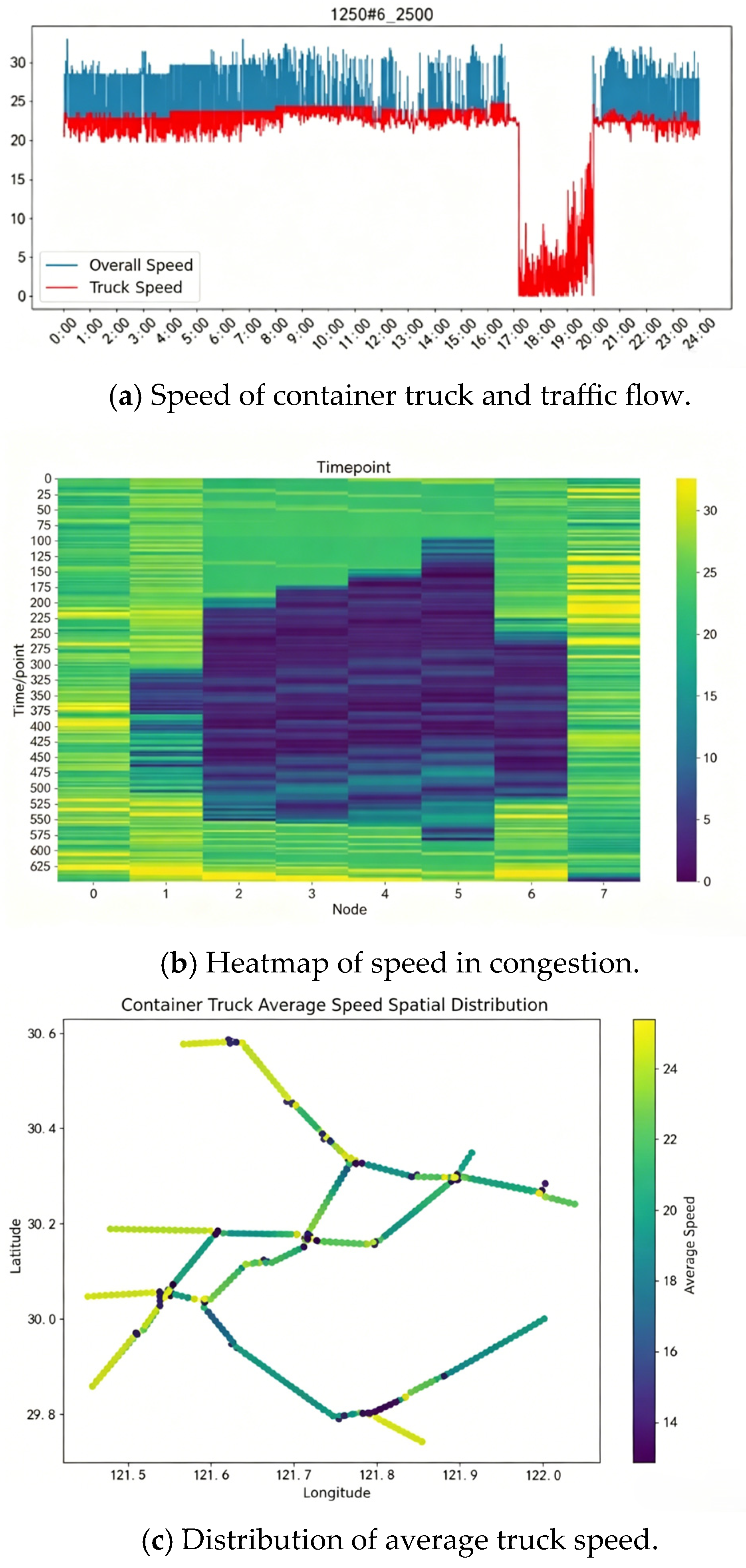
To evaluate the simulation’s usability, we conducted a comprehensive visual analysis of the simulation outputs to determine whether the generated traffic data accurately reflect real-world traffic patterns, as shown in
Figure A1.
Figure A1.
Some results of simulation.
Figure A1.
Some results of simulation.
As illustrated in
Figure A1a, container truck speeds are marginally lower than the overall average vehicle speed under free-flow conditions; during congestion, however, their speeds converge with those of other vehicle classes.
Figure A1b demonstrates the simulation’s capability to reproduce upstream propagation of congestion—a hallmark of empirically observed traffic breakdowns.
Figure A1c presents the spatial distribution of container truck speeds, revealing a clear gradient: speeds decrease proximal to the port area and increase with distance from the port, consistent with field observations.
References
- Lonza, L.; Marolda, M.C. Ports as Drivers of Urban and Regional Growth. Transp. Res. Procedia 2016, 14, 2507–2516. [Google Scholar] [CrossRef]
- Caldeira dos Santos, M.; Pereira, F.H. Development and application of a dynamic model for road port access and its impacts on port-city relationship indicators. J. Transp. Geogr. 2021, 96, 103189. [Google Scholar] [CrossRef]
- Wang, Y.; Papageorgiou, M. Real-time freeway traffic state estimation based on extended Kalman filter: A general approach. Transp. Res. Part B Methodol. 2005, 39, 141–167. [Google Scholar] [CrossRef]
- Aboudolas, K.; Geroliminis, N. Perimeter and boundary flow control in multi-reservoir heterogeneous networks. Transp. Res. Part B Methodol. 2013, 55, 265–281. [Google Scholar] [CrossRef]
- Owais, M.; Allam, A.A. Adaptive Optimization of Traffic Sensor Locations Under Uncertainty Using Flow-Constrained Inference. Appl. Sci. 2025, 15, 10257. [Google Scholar] [CrossRef]
- Owais, M.; Ahmed, A.S. Sensing the Road Ahead: Advanced Randomized Algorithm for Situational Awareness in Smart Transportation. Int. J. Comput. Intell. Appl. 2026, 25, 2641010. [Google Scholar] [CrossRef]
- Seo, T.; Bayen, A.M.; Kusakabe, T.; Asakura, Y. Traffic state estimation on highway: A comprehensive survey. Annu. Rev. Control 2017, 43, 128–151. [Google Scholar] [CrossRef]
- Xing, J.; Wu, W.; Cheng, Q.; Liu, R. Traffic state estimation of urban road networks by multi-source data fusion: Review and new insights. Phys. A Stat. Mech. Its Appl. 2022, 595, 127079. [Google Scholar] [CrossRef]
- Wackernagel, H. Ordinary Kriging. In Multivariate Geostatistics: An Introduction with Applications; Wackernagel, H., Ed.; Springer: Berlin/Heidelberg, Germany, 1995; pp. 74–81. [Google Scholar]
- Appleby, G.; Liu, L.; Liu, L.-P. Kriging convolutional networks. In Proceedings of the AAAI Conference on Artificial Intelligence, New York, NY, USA, 7–12 February 2020; Volume 34, pp. 3187–3194. [Google Scholar]
- Wu, Y.; Zhuang, D.; Labbe, A.; Sun, L. Inductive graph neural networks for spatiotemporal kriging. In Proceedings of the AAAI Conference on Artificial Intelligence, Online, 2–9 February 2021; Volume 35, pp. 4478–4485. [Google Scholar] [CrossRef]
- Liang, W.; Li, Y.; Xie, K.; Zhang, D.; Li, K.C.; Souri, A.; Li, K. Spatial-Temporal Aware Inductive Graph Neural Network for C-ITS Data Recovery. IEEE Trans. Intell. Transp. Syst. 2023, 24, 8431–8442. [Google Scholar] [CrossRef]
- Nie, T.; Qin, G.; Wang, Y.; Sun, J. Towards better traffic volume estimation: Jointly addressing the underdetermination and nonequilibrium problems with correlation-adaptive GNNs. Transp. Res. Part C Emerg. Technol. 2023, 157, 104402. [Google Scholar] [CrossRef]
- Pan, R.; Xiao, F.; Zhang, H.; Shen, M. Kriformer: A novel spatiotemporal kriging approach based on graph transformers. arXiv 2024, arXiv:2409.14906. [Google Scholar]
- Wei, T.; Lin, Y.; Guo, S.; Lin, Y.; Zhao, Y.; Jin, X.; Wu, Z.; Wan, H. Inductive and adaptive graph convolution networks equipped with constraint task for spatial–temporal traffic data kriging. Knowl.-Based Syst. 2024, 284, 111325. [Google Scholar] [CrossRef]
- Wu, Y.; Zhuang, D.; Lei, M.; Labbe, A.; Sun, L. Spatial aggregation and temporal convolution networks for real-time kriging. arXiv 2021, arXiv:2109.12144. [Google Scholar]
- Yao, X.; Gao, Y.; Zhu, D.; Manley, E.; Wang, J.; Liu, Y. Spatial Origin-Destination Flow Imputation Using Graph Convolutional Networks. IEEE Trans. Intell. Transp. Syst. 2021, 22, 7474–7484. [Google Scholar] [CrossRef]
- Zheng, C.; Fan, X.; Wang, C.; Qi, J.; Chen, C.; Chen, L. Increase: Inductive graph representation learning for spatio-temporal kriging. In Proceedings of the ACM Web Conference 2023, Austin, TX, USA, 30 April–4 May 2023; pp. 673–683. [Google Scholar]
- Yu, B.; Yin, H.; Zhu, Z. Spatio-Temporal Graph Convolutional Networks: A Deep Learning Framework for Traffic Forecasting. In Proceedings of the Twenty-Seventh International Joint Conference on Artificial Intelligence; International Joint Conferences on Artificial Intelligence Organization: Marina Del Rey, California, USA, 2018. [Google Scholar]
- Li, Y.; Yu, R.; Shahabi, C.; Liu, Y. Diffusion convolutional recurrent neural network: Data-driven traffic forecasting. arXiv 2017, arXiv:1707.01926. [Google Scholar]
- Guo, S.; Lin, Y.; Feng, N.; Song, C.; Wan, H. Attention based spatial-temporal graph convolutional networks for traffic flow forecasting. In Proceedings of the AAAI Conference on Artificial Intelligence, Honolulu, HI, USA, 27 January–1 February 2019; Volume 33, pp. 922–929. [Google Scholar]
- Roth, A.; Liebig, T. Forecasting Unobserved Node States with spatio-temporal Graph Neural Networks. In Proceedings of the 2022 IEEE International Conference on Data Mining Workshops (ICDMW), Orlando, FL, USA, 28 November–1 December 2022; IEEE: New York, NY, USA, 2022; pp. 740–747. [Google Scholar] [CrossRef]
- Mei, H.; Li, J.; Liang, Z.; Zheng, G.; Shi, B.; Wei, H. Uncertainty-aware Traffic Prediction under Missing Data. In Proceedings of the 2023 IEEE International Conference on Data Mining (ICDM), Shanghai, China, 1–4 December 2023; IEEE: New York, NY, USA, 2023; pp. 1223–1228. [Google Scholar] [CrossRef]
- Zhou, Q.; Zhang, Y.; Makridis, M.A.; Kouvelas, A.; Wang, Y.; Hu, S. MoGERNN: An inductive traffic predictor for unobserved locations. Transp. Res. Part C Emerg. Technol. 2025, 174, 105080. [Google Scholar] [CrossRef]
- Zhou, Q.; Zhang, Y.; Makridis, M.A.; Kouvelas, A.; Wang, Y.; Hu, S. Network-Wide Freeway Traffic Estimation Using Sparse Sensor Data: A Dirichlet Graph Auto-Encoder Approach. IEEE Trans. Intell. Transp. Syst. 2025, 26, 22161–22177. [Google Scholar] [CrossRef]
- Zhao, Y.; Wang, C.; Rui, Y.; Lu, W.; Ran, B. Structure-inductive meta-learning empowers partial-to-global traffic state forecasting in dynamic sensor networks. Transp. Res. Part C Emerg. Technol. 2026, 185, 105564. [Google Scholar] [CrossRef]
- Pope, J.A.; Rakes, T.R.; Rees, L.P.; Crouch, I.W.M. A Network Simulation of High-congestion Road-traffic Flows in Cities with Marine Container Terminals. J. Oper. Res. Soc. 1995, 46, 1090–1101. [Google Scholar] [CrossRef]
- Yang, Z.; Chen, G.; Moodie, D.R. Modeling road traffic demand of container consolidation in a Chinese port terminal. J. Transp. Eng. 2010, 136, 881–886. [Google Scholar] [CrossRef]
- Ziemska-Osuch, M.; Guze, S. Analysis of the Impact of Road Traffic Generated by Port Areas on the Urban Transport Network—Case Study of the Port of Gdynia. Appl. Sci. 2023, 13, 200. [Google Scholar] [CrossRef]
- Bernacki, D.; Lis, C. Traffic and freight flow predictions and effects of capacity expansion in the urban–port road interface: The case of a port city in Poland. Marit. Policy Manag. 2023, 50, 1005–1026. [Google Scholar] [CrossRef]
- Bernacki, D.; Lis, C. Exploring the Sustainable Effects of Urban-Port Road System Reconstruction. Energies 2021, 14, 6512. [Google Scholar] [CrossRef]
- Zhang, Y.; Bowden, R.; Allen, A.J. Intermodal Freight Transportation Planning Using Commodity Flow Data. 2004. Available online: https://rosap.ntl.bts.gov/view/dot/5505 (accessed on 7 July 2026).
- Xie, Y.; Huynh, N. Kernel-Based Machine Learning Models for Predicting Daily Truck Volume at Seaport Terminals. J. Transp. Eng. 2010, 136, 1145–1152. [Google Scholar] [CrossRef]
- Kourounioti, I.; Polydoropoulou, A.; Tsiklidis, C. Development of Models Predicting Dwell Time of Import Containers in Port Container Terminals—An Artificial Neural Networks Application. Transp. Res. Procedia 2016, 14, 243–252. [Google Scholar] [CrossRef]
- Gao, Y.; Chang, D.; Fang, T.; Fan, Y. The Daily Container Volumes Prediction of Storage Yard in Port with Long Short-Term Memory Recurrent Neural Network. J. Adv. Transp. 2019, 2019, 5764602. [Google Scholar] [CrossRef]
- Luo, Y.; Huang, L. Port Short-Term Truck Flow Forecasting Model Based on Wavelet Neural Network. In Proceedings of the 2020 International Conference on Intelligent Transportation, Big Data & Smart City (ICITBS), Vientiane, Laos, 11–12 January 2020; IEEE: New York, NY, USA, 2020; pp. 43–47. [Google Scholar] [CrossRef]
- Nadi, A.; Sharma, S.; Snelder, M.; Bakri, T.; van Lint, H.; Tavasszy, L. Short-term prediction of outbound truck traffic from the exchange of information in logistics hubs: A case study for the port of Rotterdam. Transp. Res. Part C Emerg. Technol. 2021, 127, 103111. [Google Scholar] [CrossRef]
- Li, N.; Sheng, H.; Wang, P.; Jia, Y.; Yang, Z.; Jin, Z. Modeling Categorized Truck Arrivals at Ports: Big Data for Traffic Prediction. IEEE Trans. Intell. Transp. Syst. 2023, 24, 2772–2788. [Google Scholar] [CrossRef]
- Vaswani, A.; Shazeer, N.; Parmar, N.; Uszkoreit, J.; Jones, L.; Gomez, A.N.; Kaiser, Ł.; Polosukhin, I. Attention is all you need. In Advances in Neural Information Processing Systems; AAAI Press: Menlo Park, CA, USA, 2017; Volume 30. [Google Scholar]
- Ekambaram, V.; Jati, A.; Nguyen, N.; Sinthong, P.; Kalagnanam, J. TSMixer: Lightweight MLP-Mixer Model for Multivariate Time Series Forecasting. In Proceedings of the 29th ACM SIGKDD Conference on Knowledge Discovery and Data Mining, Long Beach, CA, USA, 6–10 August 2023; pp. 459–469. [Google Scholar] [CrossRef]
- Fan, J.; Shen, Y. StockMixer: A simple yet strong MLP-based architecture for stock price forecasting. In Proceedings of the AAAI Conference on Artificial Intelligence, Vancouver, BC, Canada, 20–27 February 2024; Volume 38, pp. 8389–8397. [Google Scholar]
- Xie, Y.; Xiong, Y.; Gao, X.; Chen, J.; Zhang, Y.; Wu, X.; Chen, C. LAMEE: A light all-MLP framework for time series prediction empowering recommendations. World Wide Web 2024, 27, 13. [Google Scholar] [CrossRef]
- Seo, T. UXsim: Lightweight mesoscopic traffic flow simulator in pure Python. J. Open Source Softw. 2025, 10, 7617. [Google Scholar] [CrossRef]
- Kipf, T.N.; Welling, M. Semi-supervised classification with graph convolutional networks. arXiv 2016, arXiv:1609.02907. [Google Scholar]
- Nie, T.; Qin, G.; Wang, Y.; Sun, J. Correlating sparse sensing for large-scale traffic speed estimation: A Laplacian-enhanced low-rank tensor kriging approach. Transp. Res. Part C Emerg. Technol. 2023, 152, 104190. [Google Scholar] [CrossRef]
| Disclaimer/Publisher’s Note: The statements, opinions and data contained in all publications are solely those of the individual author(s) and contributor(s) and not of MDPI and/or the editor(s). MDPI and/or the editor(s) disclaim responsibility for any injury to people or property resulting from any ideas, methods, instructions or products referred to in the content. |




 and
and