Decoupling Economic Growth from CO₂ Emissions in Honduras: A Longitudinal Machine-Learning and Econometric Assessment of Low-Carbon Development, 1990–2023

Abstract

Decoupling economic growth from CO₂ emissions is a key challenge for developing economies, with limited evidence for small Central American economies. This study evaluates Honduras during 1990–2023 using GDP per capita, CO₂ emissions per capita, energy intensity, and renewable energy share from World Bank Indicators and the Global Carbon Project. The methodology integrates k-means clustering, PELT structural break detection, the Tapio decoupling index, Environmental Kuznets Curve (EKC) modelling, Granger causality, and Random Forest analysis. Since energy-intensity data are available only from 2000, a full GDP-CO₂ series (1990–2023, n = 34) is distinguished from a complete four-variable panel (2000–2021, n = 22). Clustering identifies two structural regimes rather than three (silhouette 0.490 vs. 0.476). EKC results support an inverted-U relationship (β₂ = −3.012, p < 0.001; adjusted R² = 0.766), with an estimated turning point of USD 2388 (95% CI: USD 2156–2644, delta method), near the upper boundary of the estimation sample, which Honduras’ 2023 GDP per capita (USD 2527) marginally exceeds as an out-of-sample extrapolation. However, Granger tests find no significant temporal precedence between GDP, renewable share, and CO₂ emissions (all p > 0.05), and Random Forest shows GDP per capita (%IncMSE = 31.47) vastly outweighs renewable share (%IncMSE = 0.16). Honduras has likely crossed the EKC threshold, but evidence does not support a renewable-driven decoupling.

1. Introduction

1.1. General Considerations

The tension between economic growth and environmental degradation remains one of the central challenges of contemporary sustainable development. Since the Brundtland Report by the World Commission on Environment and Development (WCED), sustainability debates have emphasized the need for development trajectories that allow economic progress without compromising environmental quality or the well-being of future generations [1].

In energy-dependent economies, this challenge is especially relevant because economic expansion has historically been associated with higher energy consumption, increased fossil-fuel use, and rising carbon dioxide (CO₂) emissions [2]. In this context, decoupling refers to the weakening or rupture of the proportional relationship between economic growth and environmental pressure. Relative decoupling occurs when emissions continue to increase but at a slower rate than gross domestic product (GDP), whereas absolute decoupling occurs when GDP grows while emissions decline. The Tapio decoupling index provides an elasticity-based framework to classify these relationships and has been widely applied in studies of economic growth and CO₂ emissions [3]. However, decoupling outcomes depend on the environmental indicator selected, the time horizon, and the territorial scale considered [4]. Therefore, country-specific assessments remain necessary, particularly for economies with distinctive energy transitions and limited empirical evidence.

Honduras provides a relevant case for evaluating economic growth–CO₂ emissions decoupling. It is a small, open, lower-middle-income economy in Central America whose energy system has undergone major structural changes during the last three decades. The country experienced a period of fossil-fuel thermal expansion, followed by a partial recovery of renewable electricity generation through hydropower, solar photovoltaic, wind, and biomass resources [5,6,7]. These changes occurred in a context marked by electricity losses, imported fuel dependence, financial constraints in the power sector, and the need for long-term energy planning, [8,9]. Understanding whether this historical transition has translated into measurable decoupling between GDP per capita and CO₂ emissions per capita is therefore relevant for climate-policy monitoring and low-carbon development planning.

The Environmental Kuznets Curve (EKC) hypothesis proposes an inverted-U relationship between income per capita and environmental degradation. According to this hypothesis, environmental pressure initially increases with economic growth but may decline after a certain income threshold [10,11]. Nevertheless, empirical evidence remains mixed and strongly dependent on the pollutant, country group, model specification, and time horizon considered [12,13]. For this reason, the EKC should not be interpreted as automatic evidence of sustainable development. In this study, the EKC is used as one component of a broader empirical framework that also includes decoupling analysis, structural break detection, clustering, temporal causality, and machine learning.

Machine learning (ML) methods can complement conventional econometric approaches by identifying nonlinear patterns, structural groupings, and variable importance in multidimensional datasets [14]. In this study, k-means clustering, Pruned Exact Linear Time (PELT) structural break detection, and Random Forest analysis are integrated with the Tapio index, EKC modelling, and Granger causality tests to evaluate Honduras’ trajectory during 1990–2023 [15,16]. The study addresses four research questions: (i) What structural regimes characterize Honduras’ 1990–2023 development trajectory? (ii) Is there evidence consistent with an EKC-type relationship between GDP per capita and CO₂ emissions per capita, and what is the estimated turning point? (iii) Do changes in renewable energy share or GDP per capita statistically precede changes in CO₂ emissions per capita? and (iv) Which variables best explain the trajectory of CO₂ emissions per capita under an exploratory machine-learning framework? Research question (i) is addressed descriptively using the long-run GDP-CO₂ series (Panel A, 1990–2023, n = 34); research questions (i)–(iv) are addressed in their multivariate form using the complete four-variable panel (Panel B, 2000–2021, n = 22).

1.2. State of the Art

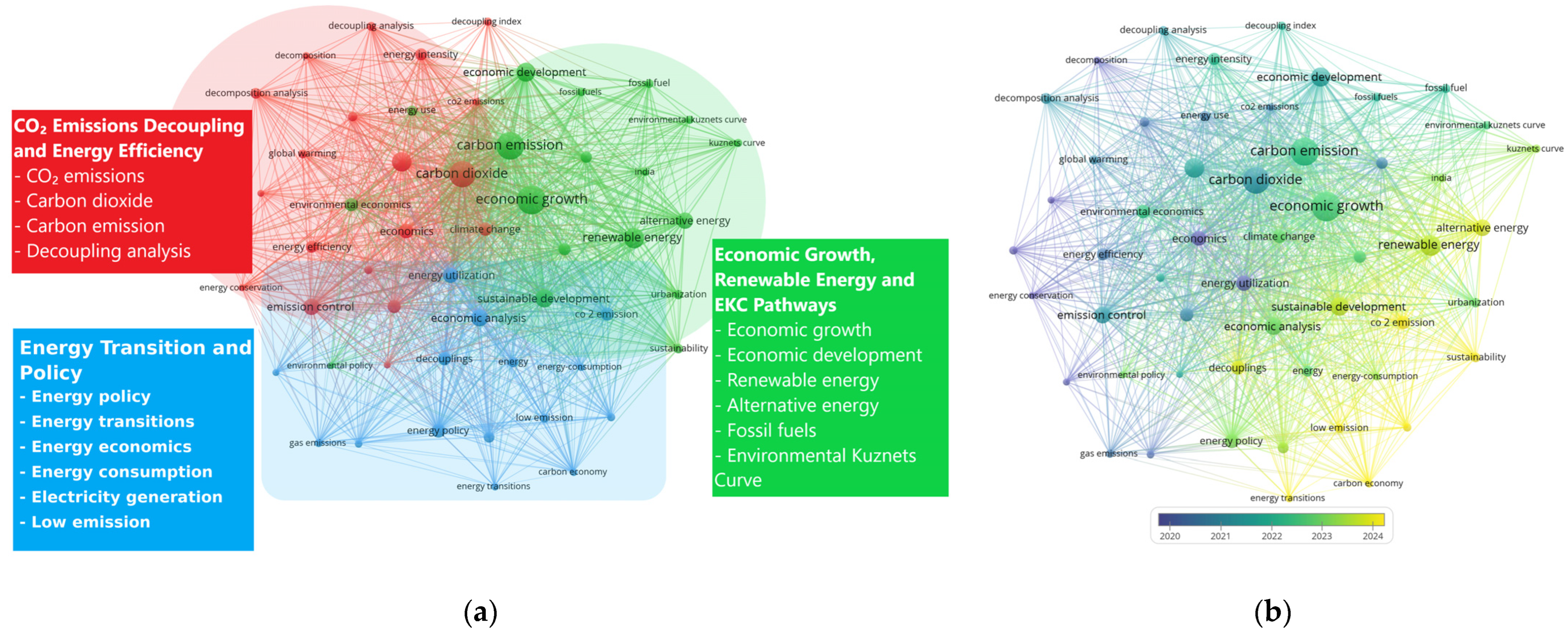
Before reviewing the literature in detail, a bibliometric analysis was conducted to contextualize the research field. Figure 1 presents a keyword mapping of the reviewed literature. Panel (a) identifies three main thematic areas: CO₂ emissions decoupling and energy efficiency, economic growth and renewable energy pathways, and energy policy and transition dynamics. Panel (b) shows the temporal evolution of keywords, indicating that recent studies, particularly those conducted close to 2024, are increasingly associated with renewable energy, sustainability, low-carbon development, and energy-transition pathways.

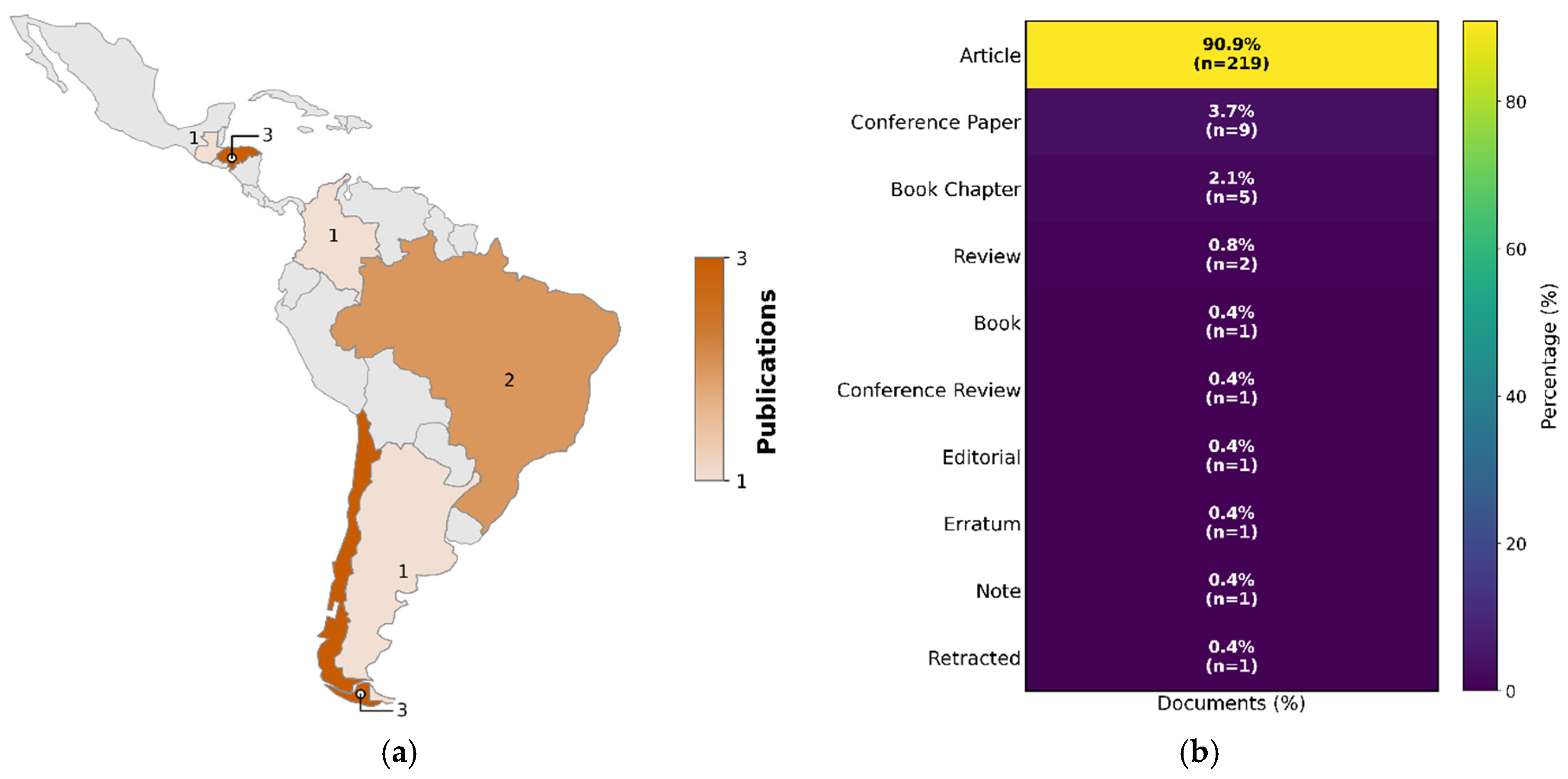
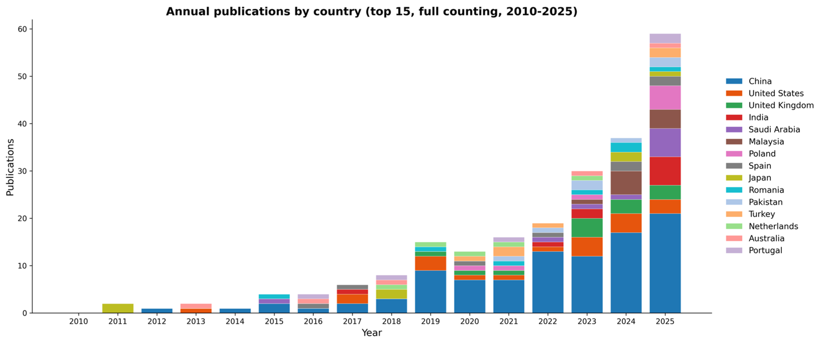
Figure 2 shows the annual publication trend for the top 15 contributing countries during 2010–2025. The results indicate a clear increase in scientific output after 2018, with stronger growth in the most recent years. China dominates the field, followed by the United States and the United Kingdom, while India, Saudi Arabia, Malaysia, Poland, Spain, Japan, Romania, Pakistan, Turkey, the Netherlands, Australia, and Portugal also contribute to the literature. Figure 3 summarizes the regional and document-type distribution. In Latin America, the contribution remains limited, with Chile and Honduras showing the highest representation, followed by Brazil, Argentina, Colombia, and Guatemala. The document-type classification shows that the reviewed literature is dominated by journal articles, supporting the academic consistency of the evidence base.

The literature on economic growth–CO₂ emissions decoupling has expanded substantially in recent years. The Tapio elasticity index has been widely used to classify decoupling states between economic activity and environmental pressure. Hao et al. [17] combined Tapio’s model with EKC analysis to examine whether carbon emissions and economic growth decouple across Chinese provinces. Tong and Sun [4] further showed that decoupling outcomes are sensitive to the selected indicator, analytical scale, and time window. These studies support the use of Tapio’s index in the present research and justify the focus on CO₂ emissions per capita as the primary environmental pressure variable, while carbon intensity is retained as a complementary indicator.

The EKC literature also provides relevant but inconclusive evidence. In Latin America and the Caribbean, Al-Mulali et al. [18] found evidence consistent with an inverted-U relationship between gross domestic product (GDP) and CO₂ emissions. Conversely, Zilio and Caraballo [19] rejected the existence of a Carbon Kuznets Curve in the region and argued that “grow first, clean later” is not a suitable strategy for Latin American economies. This contrast indicates that the EKC results should be interpreted cautiously and complemented with additional evidence on decoupling states, structural changes, and renewable energy dynamics.

Renewable energy has been identified as a key mechanism for reducing CO₂ emissions, although its impact varies across regions, institutions, and technologies [20]. Akram et al. [21] showed that renewable energy and energy efficiency reduce emissions in developing countries, while Yao et al. [22] argued that renewable energy adoption can accelerate the EKC turning point by changing the energy structure. However, Ahmed and Shimada [23] found that Latin American and Caribbean economies still rely strongly on non-renewable energy for economic growth. Therefore, the effect of renewable energy on emissions reduction should be empirically evaluated in each national context.

The energy–growth–emissions nexus is dynamic and may change over time. Shahbaz et al. [24] showed that causal relationships among economic growth, energy use, and CO₂ emissions are not necessarily stable, while Leiva and Rubio-Varas [25] found substantial heterogeneity in the energy–GDP relationship across Latin American countries. For Honduras, Amaya Sarmiento and Paredes Heller [26] analyzed GDP, electricity consumption, CO₂ emissions, financial development, and government expenditure using a vector autoregression model. Their study provides valuable national evidence, but it does not explicitly evaluate decoupling states, structural eras, or renewable-driven regime shifts.

The Honduran energy-policy literature also supports the need for a country-specific assessment. Flores et al. [27] identified fossil-fuel dependence, electricity losses, financial constraints, and weak long-term energy planning as key challenges for Honduras. Later, Flores [9] showed that after 2009 the Honduran electricity sector experienced reforms, photovoltaic incentives, increased renewable investment, and institutional restructuring. More recently, Pineda-Guzman et al. [28] evaluated future pathways for decarbonizing Honduras’ power sector. However, these studies focus mainly on policy diagnosis or prospective scenarios, while limited evidence exists on whether Honduras’ historical energy transition has already produced measurable economic growth–CO₂ emissions decoupling, and on the statistical robustness of such evidence given data constraints.

Three main gaps therefore remain. First, most growth–CO₂ decoupling studies focus on large economies, global panels, or regional aggregates, leaving small Central American economies underexplored. Second, Latin American evidence on the EKC and renewable energy remains mixed, requiring country-specific validation. Third, existing studies on Honduras have not integrated decoupling analysis, EKC modelling, structural break detection, clustering, Granger causality, and machine learning within a single longitudinal framework that also transparently addresses the limitations of short annual panels.

1.3. Motivation and Contributions

Honduras is a relevant case for studying economic growth–CO₂ emissions decoupling because its energy system has experienced both fossil-fuel thermal expansion and later renewable energy diversification. However, it remains unclear whether these structural changes have translated into measurable, statistically robust decoupling between GDP per capita and CO₂ emissions per capita. Addressing this question is important not only for Honduras, but also for comparable Central American economies seeking to reconcile economic development, renewable energy expansion, and climate-policy commitments. This study makes three main contributions. First, it provides a country-specific empirical assessment of economic growth–CO₂ emissions decoupling in Honduras using verified data from primary international sources (World Bank WDI and the Global Carbon Project), explicitly distinguishing the data coverage available for each variable rather than assuming a uniform panel. Second, it integrates the Tapio decoupling index, EKC modelling, PELT structural break detection, k-means clustering, Granger causality, and Random Forest analysis within a single longitudinal framework, with statistical safeguards appropriate for a short annual panel (n = 22 for the complete four-variable analysis). Third, it offers a methodologically transparent discussion of why structural-level predictors (GDP per capita) and temporal-precedence tests (Granger causality on renewable energy share) can yield seemingly contrasting conclusions, and what this implies for climate-policy design in Honduras.

By combining rigorous empirical analysis with energy-policy interpretation, this study contributes to the literature on sustainable development in small and climate-vulnerable economies. It also provides a methodological framework, including explicit documentation of data coverage limitations, that can be replicated in other Central American countries to compare decoupling trajectories and support evidence-based climate governance.

2. Materials and Methods

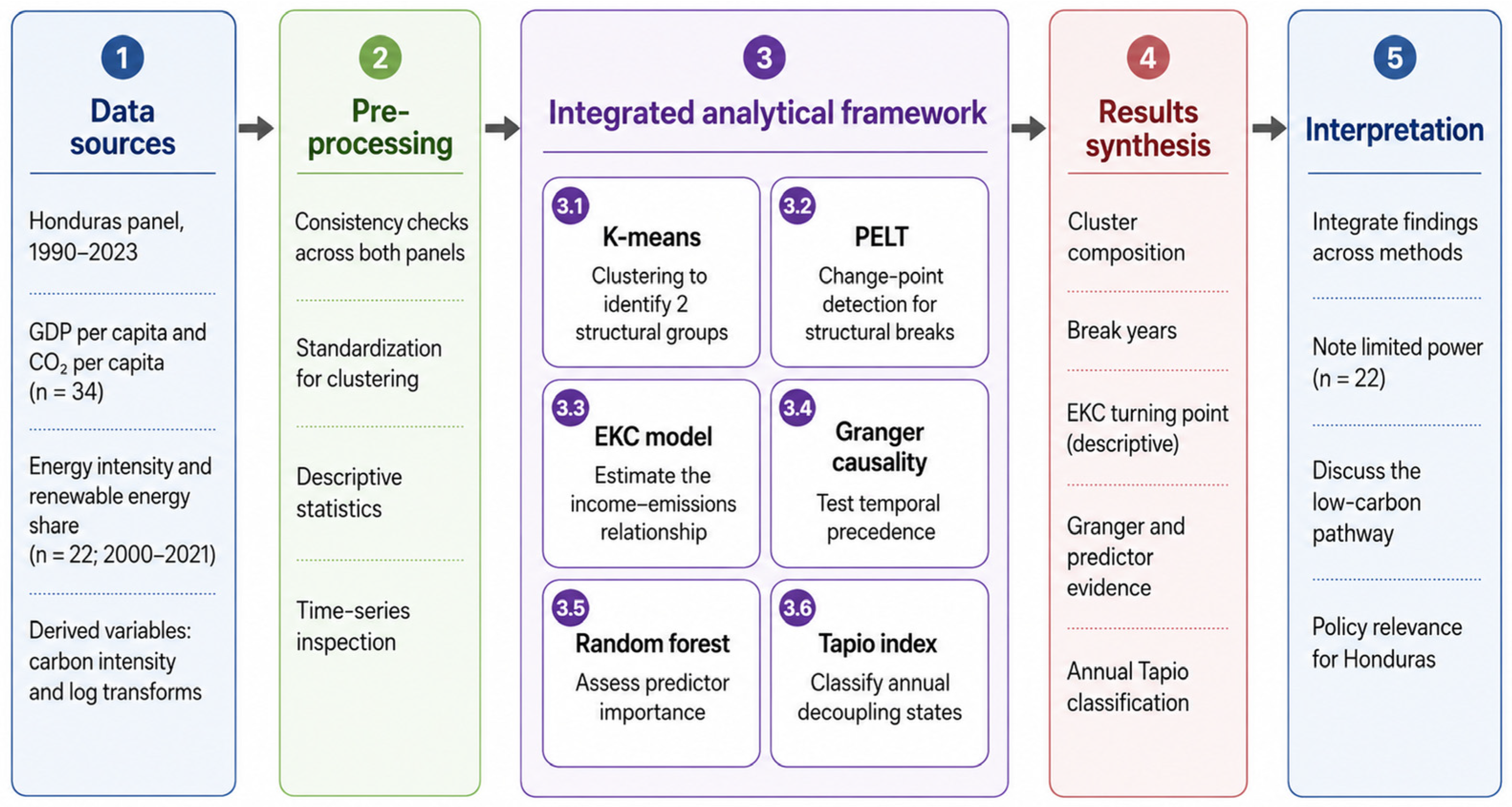
This section describes the methodological framework used to assess the relationship between economic growth, CO₂ emissions, energy intensity, and renewable energy deployment in Honduras during 1990–2023. The analysis followed a sequential workflow including data compilation, variable preprocessing, exploratory analysis, structural regime identification, structural break detection, econometric modelling, temporal precedence testing, machine-learning assessment, and decoupling classification. Because complete four-variable coverage is available only from 2000 onward, descriptive components of the workflow draw on the full 1990–2023 GDP–CO₂ series (Panel A, n = 34), while structural regime identification, structural break detection, econometric modelling, temporal precedence testing, machine-learning assessment, and decoupling classification are based on the complete four-variable panel (Panel B, 2000–2021, n = 22). Figure 4 summarizes the methodological workflow applied in this study.

2.1. Data Sources and Variables

An annual dataset was constructed for Honduras covering the period 1990–2023. Data were obtained directly from two verified primary sources: the World Bank World Development Indicators (WDI) database, accessed on 20 June 2026, for GDP per capita, energy intensity, and renewable energy share; and Our World in Data’s processed series of the Global Carbon Project’s Global Carbon Budget, accessed on 20 June 2026, for CO₂ emissions per capita [29,30].

Table 1. Variables used in the Honduras annual panel, 1990–2023.

Variable	Description	Unit	Source	Code/Reference
GDP per capita	Gross domestic product per inhabitant, constant 2015 USD	USD/inhabitant	World Bank WDI	NY.GDP.PCAP.KD
CO2 per capita	CO2 emissions per inhabitant	t CO2/inhabitant	OWID/Global Carbon Project	Emissions total per capita
Energy intensity	Primary energy use per unit of GDP (PPP)	MJ/USD	World Bank WDI	EG.EGY.PRIM.PP.KD
Renewable energy share	Renewable electricity output (share of total electricity generation)	%	World Bank WDI	EG.ELC.RNEW.ZS
Carbon intensity	CO2 emissions per unit of GDP	kg CO2/USD	Derived	CO2_pc/GDP_pc × 1000
ln(GDP pc)	Natural logarithm of GDP per capita	—	Derived	ln(NY.GDP.PCAP.KD)
[ln(GDP pc)]2	Quadratic term for EKC estimation	—	Derived	[ln(NY.GDP.PCAP.KD)]2

Variables used in the Honduras annual dataset, 1990–2023. WDI = World Development Indicators; OWID = Our World in Data. Source: Own elaboration based on data downloaded from https://databank.worldbank.org and https://ourworldindata.org/grapher/co-emissions-per-capita on 20 June 2026 [29,30].

presents the variables used in the analysis, including their description, units, sources, and reference codes.

Critically, data coverage differs across variables. GDP per capita and CO₂ per capita are available for the full 1990–2023 period (34 annual observations, no missing values). However, renewable energy share is available only for 1990–2021 (32 of 34 years; 2022–2023 missing), and energy intensity is available only from 2000 onward (22 of 34 years; 1990–1999 and 2022–2023 missing), reflecting the limited historical reporting of energy statistics for small Central American economies in international databases.

Table 2. Data coverage by variable, Honduras 1990–2023.

Variable	Years Available	Years Missing
GDP per capita	34 (1990–2023)	0
CO2 per capita	34 (1990–2023)	0
Renewable energy share	32 (1990–2021)	2 (2022–2023)
Energy intensity	22 (2000–2021)	12 (1990–1999, 2022–2023)

summarizes this coverage.

To address this asymmetric coverage, two analytical panels are defined. Panel A (1990–2023, n = 34) includes only GDP per capita and CO₂ per capita, both fully observed, and is used for descriptive trends and the annual Tapio decoupling index. Panel B (2000–2021, n = 22) includes all four variables with no missing values, and is used for k-means clustering, PELT structural break detection, EKC estimation, Granger causality testing, and Random Forest analysis, all of which require complete observations across variables. This dual-panel strategy avoids both data imputation and the silent exclusion of incomplete years, preserving the full 1990–2023 record where the underlying variables allow it.

Carbon intensity was calculated as

$${CI}_T={\displaystyle \frac{{CO}_{2pc,t}}{{GDP}_{pc,t}}}\times 1000$$

(1)

where $C{I}_t$ is carbon intensity in year $t$, $C{O}_{2pc,t}$ is CO₂ emissions per capita, and $GD{P}_{pc,t}$ is GDP per capita.

2.2. Methodological Workflow

All analyses were conducted in R version 4.5.3. Before applying the models, both panels were checked for consistency and inspected using descriptive statistics and time-series visualization. Variables used in the clustering stage (Panel B) were standardized using z-score normalization to ensure comparability across indicators with different units.

The standardization was performed as

$$z_{i,j}={\displaystyle \frac{x_{ij}-\overline{x_j}}{s_j}}$$

(2)

where $z_{ij}$ is the standardized value of observation $i$ for variable $j$, $x_{ij}$ is the original value, ${\bar{x}}_j$ is the mean of variable $j$, and $s_j$ is its standard deviation.

First, k-means clustering was applied to Panel B to identify structural regimes based on the joint behaviour of economic, energy, and environmental variables. The clustering algorithm minimizes the within-cluster sum of squares, defined as

$$J={\displaystyle \sum _{k=1}^K}\sum _{i\in C_k}{‖x_i-{\mu }_k‖}^2$$

(3)

where $J$ is the clustering objective function, $K$ is the number of clusters, $C_k$ is cluster $k$, $x_i$ is the standardized annual observation, and ${\mu }_k$ is the centroid of cluster $k$. The optimal number f clusters was evaluated using the elbow method and the average silhouette criterion across k = 2 to k = 7, where the maximum admissible was n = 22 [31].

Second, the Pruned Exact Linear Time (PELT) algorithm was applied to Panel B to detect structural breaks in CO₂ emissions per capita, energy intensity, and renewable energy share. The method identifies breakpoints by minimizing a penalized cost function:

$$min\left[{\displaystyle \sum _{m=0}^M}C\left(y_{{\tau }_m}+{1:}_{{\tau }_{m+1}}\right)+\beta \right]$$

(4)

where $C(\cdot )$ is the cost function for each segment, ${\tau }_m$ represents the detected breakpoint, $M$ is the number of breakpoints, and $\beta$ is the penalty term. A Bayesian Information Criterion penalty and a minimum segment length of three years were applied to avoid spurious breakpoints.

Third, the Environmental Kuznets Curve (EKC) model was estimated on Panel B to evaluate whether the relationship between income and emissions follows an inverted-U pattern. The model was specified as

$$\ln ({CO}_{2 pc})={\beta }_0+{\beta }_1\ln \left({GDP}_{pc}\right)+{\beta }_2{\left[\ln \left({GDP}_{pc}\right)\right]}^2+\epsilon$$

(5)

where $C{O}_{2pc}$ denotes CO₂ emissions per capita, $GD{P}_{pc}$ denotes GDP per capita, ${\beta }_0$ is the intercept, ${\beta }_1$ is the linear income coefficient, ${\beta }_2$ is the quadratic income coefficient, and $\epsilon$ is the error term. Evidence consistent with an EKC-type relationship is identified when ${\beta }_1>0$ and ${\beta }_2<0$.

As a separate diagnostic step, unit root and cointegration tests for the EKC relationship were additionally conducted using the longer Panel A series (GDP and CO₂ per capita only, 1990–2023, n = 34), which affords greater statistical power for these stationarity tests than Panel B; full results are reported in Table S1 of the Supplementary Material. This diagnostic use of Panel A is distinct from, and does not replace, the Panel B estimation of Equation (5) reported in Section 3.4.

The EKC turning point was calculated as

$${GDP}^{\ast }=\exp \left(-{\displaystyle \frac{{\beta }_1}{2{\beta }_2}}\right)$$

(6)

where $GD{P}^{\ast }$ represents the estimated income turning point. The model was estimated using ordinary least squares. Newey–West heteroscedasticity- and autocorrelation-consistent standard errors were computed throughout for robustness, and serial autocorrelation and heteroscedasticity were assessed using the Durbin–Watson and Breusch–Pagan tests, respectively (results reported in Section 3.4).

Fourth, Granger temporal precedence tests were applied to Panel B, using first-differenced series given non-stationarity in levels, to evaluate whether changes in GDP per capita or renewable energy share statistically precede changes in CO₂ emissions per capita (and vice versa). The general test equation was specified as

$${\Delta CO}_{2pc,t}={\alpha }_0+{\displaystyle \sum _{i=1}^p}{\alpha }_i{\Delta CO}_{2pc,t-i}+{\displaystyle \sum _{i=1}^p}{\gamma }_i{\Delta X}_{t-i}+u_t$$

(7)

where $\Delta C{O}_{2pc,t}$ is the first difference in CO₂ emissions per capita, X represents either GDP per capita or renewable energy share, p is the lag length selected by the Akaike Information Criterion (capped at lag.max = floor(n/5) to preserve degrees of freedom given the short panel), and u_t is the error term. Equation (7) was estimated bidirectionally for each variable pair, i.e., with CO₂ emissions per capita as the dependent variable and as the explanatory variable, in turn yielding the five temporal precedence relationships reported in Section 3.5 (GDP→CO₂, CO₂→GDP, renewables→CO₂, CO₂→renewables, and GDP→renewables). The tests were interpreted strictly as temporal precedence, not as structural or counterfactual causality.

Fifth, a Random Forest model was implemented in Panel B as an exploratory machine-learning approach to assess the relative importance of the explanatory variables in predicting CO₂ emissions per capita, following the ensemble learning framework proposed by Breiman [32]. The model used 500 trees, with the number of variables tried at each split selected via 5-fold cross-validation (which, with n = 22, allocates approximately four observations per fold; results should accordingly be interpreted as exploratory). As a robustness check, the model was re-estimated using a rolling-origin cross-validation scheme (caret time slice [33]: initial Window = 14; horizon = 2; expanding window) that respects temporal ordering. Under rolling-origin validation, out-of-fold performance is lower than under 5-fold CV (R² = 0.400; RMSE = 0.073; versus R² = 0.644; RMSE = 0.056), reflecting the added difficulty of predicting genuinely unseen years—particularly 2015, the historical peak in CO₂ per capita, which no prior-year training window could anticipate. GDP per capita nonetheless remains the dominant predictor under both schemes (%IncMSE = 28.71% under rolling-origin versus 31.47% under 5-fold CV), confirming that its dominance is not an artefact of the cross-validation scheme (Supplementary Table S5). Variable importance was measured using the percentage increase in mean squared error after permutation, following the standard permutation-importance procedure implemented in the random Forest package: for each predictor j, the values of that variable are randomly permuted across observations, the resulting increase in prediction error is computed for every tree in the forest, and the average increase is normalized by its standard deviation across trees to obtain %IncMSE_j [32]. Higher values of %IncMSE_j indicate greater importance of variable j for predicting CO₂ emissions per capita.

Finally, the Tapio decoupling index was calculated on Panel A (1990–2023) annually, and aggregated by structural regime and for the full period, to classify the relationship between GDP growth and changes in CO₂ emissions:

$$e=\left({\displaystyle \frac{{\%\Delta CO}_{2pc}}{{\%\Delta GDP}_{pc}}}\right)$$

(8)

where $e$ is the decoupling elasticity, $\%\Delta C{O}_{2pc}$ is the percentage change in CO₂ emissions per capita, and $\%\Delta GD{P}_{pc}$ is the percentage change in GDP per capita. The classification followed the standard Tapio taxonomy: strong decoupling when $e<0$, weak decoupling when $0\le e<0.8$, coupled growth when $0.8\le e\le 1.2$, and expansive coupling when $e>1.2$. Because the annual elasticity is undefined when %ΔGDPpc approaches zero, years in which the GDP growth rate fell below 0.1% in absolute value were flagged and are reported separately rather than allowed to distort the visual scale of the annual series (Section 3.7).

Together, these methods provide a complementary assessment of Honduras’ long-term economic growth–CO₂ emissions trajectory. The clustering identifies structural regimes, PELT detects temporal breakpoints, the EKC evaluates the nonlinear income–emissions relationship, Granger tests assess temporal precedence, Random Forest identifies relevant predictors, and the Tapio index formally classifies decoupling states.

3. Results

3.1. Descriptive Trends

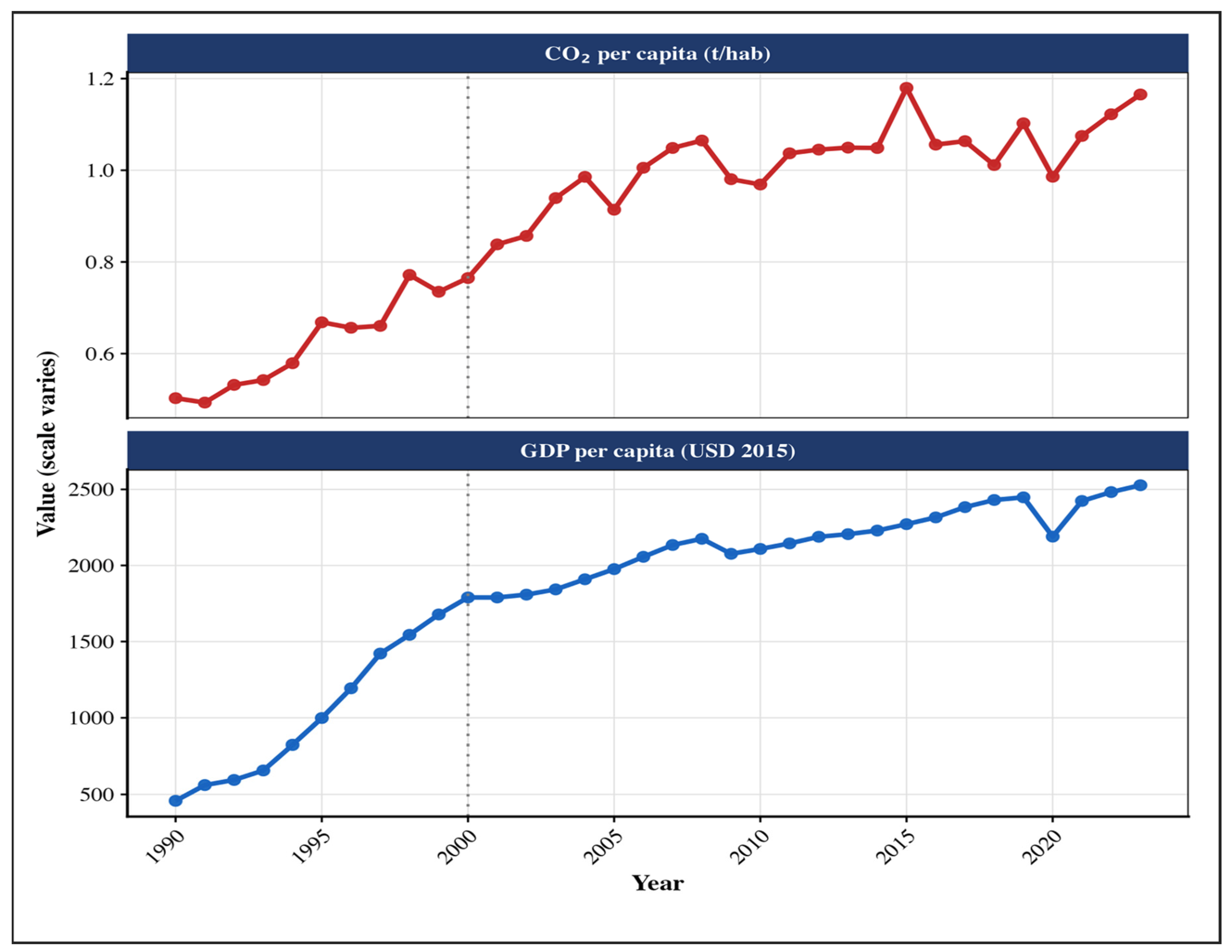
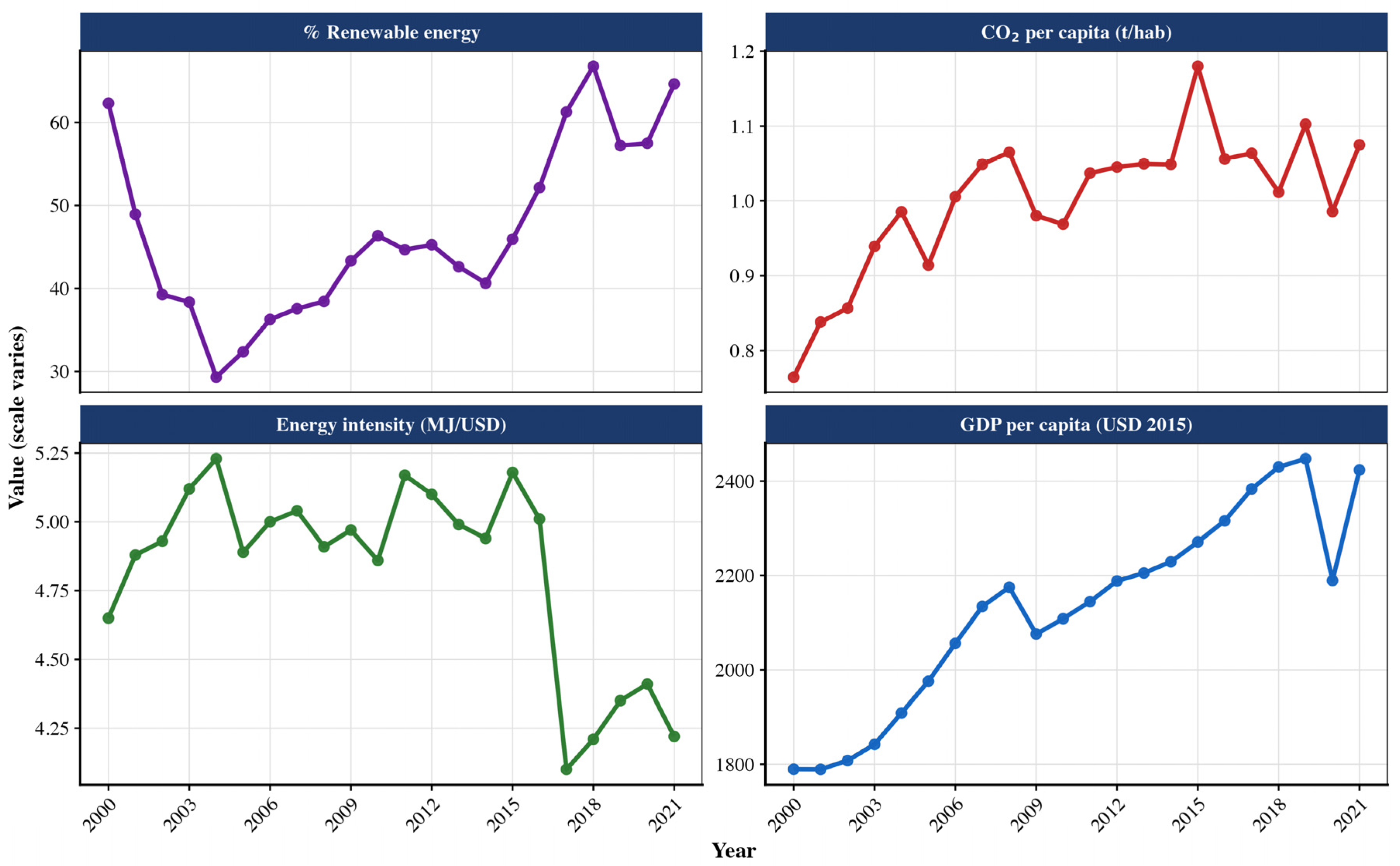
Figure 5 presents the long-run series of GDP per capita and CO₂ emissions per capita, Honduras, 1990–2023 (Panel A). The dotted vertical line marks the start of the complete four-variable panel used in subsequent analyses (2000). Figure 6 summarizes the complete four-variable panel, Honduras, 2000–2021 (Panel B): GDP per capita, CO₂ per capita, energy intensity, and renewable energy share.

GDP per capita rose from approximately USD 458 in 1990 to USD 2527 in 2023 (Panel A, n = 34), a sustained, near-monotonic increase interrupted mainly by the 2020 COVID-19 shock. CO₂ emissions per capita followed a broadly increasing but non-linear trajectory, rising from approximately 0.50 t CO₂/capita in 1990 to a first local high near 1.06 t CO₂/capita around 2007–2008, declining moderately during 2009–2010, then rising again to reach its overall peak of approximately 1.18 t CO₂/capita in 2015 and fluctuating thereafter to reach 1.17 t CO₂/capita in 2023.

Table 3. Descriptive statistics of the complete four-variable panel, Honduras 2000–2021 (Panel B).

Variable	n	Mean	SD	Min.	Max.
GDP per capita (constant 2015 USD)	22	2131.51	209.37	1789.19	2447.62
CO2 per capita (t CO2/capita)	22	1.00	0.09	0.76	1.18
Energy intensity (MJ/USD)	22	4.82	0.34	4.10	5.23
Renewable energy share (%)	22	46.85	10.70	29.31	66.76
Carbon intensity (kg CO2/USD)	22	0.47	0.03	0.42	0.52

Note: SD = standard deviation.

reports descriptive statistics for Panel B (2000–2021, n = 22), the dataset used in all subsequent multivariate analyses. GDP per capita averaged USD 2131.51 (SD = 209.37), CO₂ per capita averaged 1.00 t/capita (SD = 0.09), energy intensity averaged 4.82 MJ/USD (SD = 0.34), and renewable energy share averaged 46.85% (SD = 10.70).

3.2. Structural Regime Identification

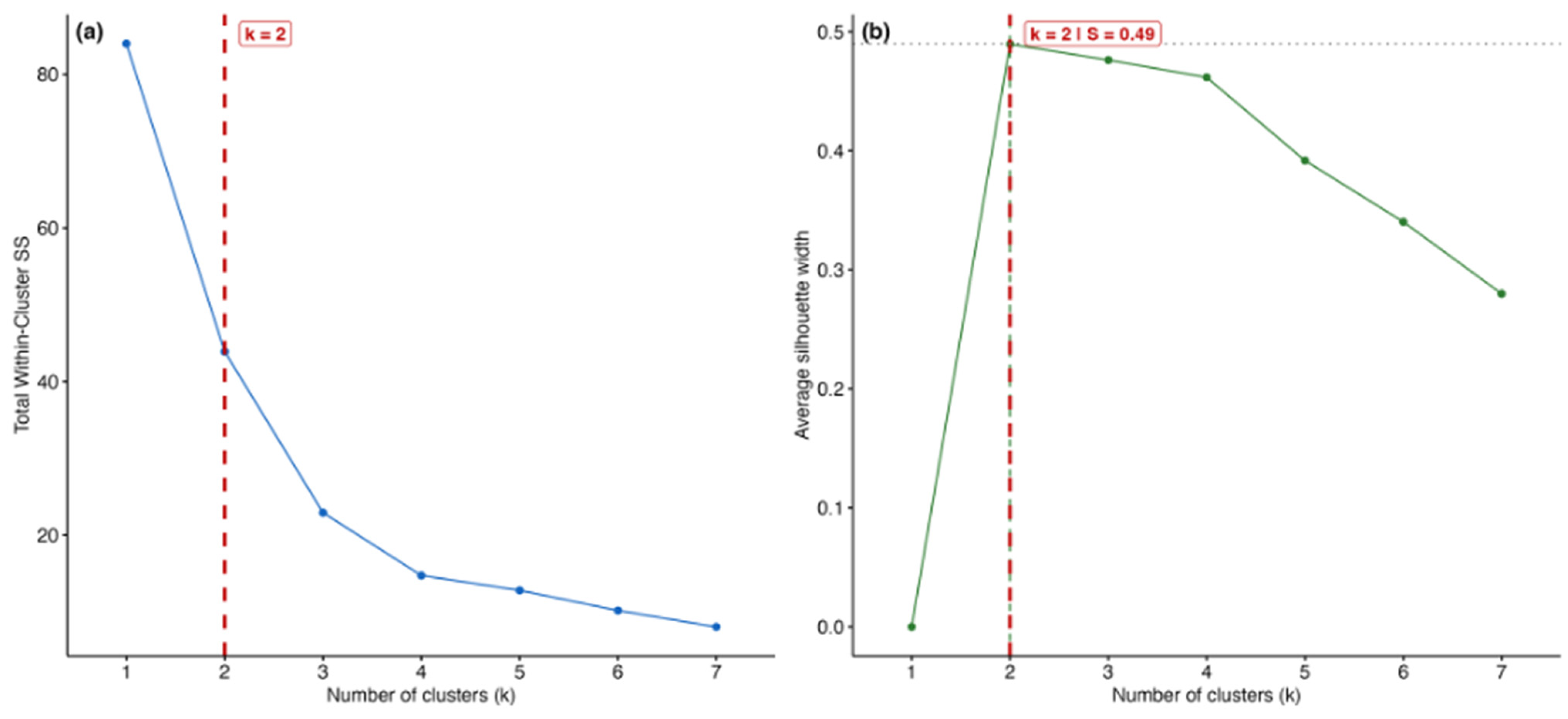
Figure 7 introduces the statistical basis for selecting the number of clusters. The elbow method and average silhouette criterion were evaluated for k = 2 to k = 7. The average silhouette width was highest at k = 2 (${\displaystyle {\mathrm{S}}^{¯}}$ = 0.490), followed closely by k = 3 (${\displaystyle {\mathrm{S}}^{¯}}$ = 0.476), with both values within a margin commonly regarded as a weak-to-moderate preference. Given that the silhouette criterion identified k = 2 as marginally superior, and consistent with avoiding the imposition of a pre-specified number of structural eras, the k = 2 solution was retained for the main analysis. This configuration explains 47.7% of the between-cluster variance (WCSS = 43.89 at k = 2).

Table 4. K-means cluster centroids (k = 2), Honduras 2000–2021 (Panel B).

Cluster	Period	n	GDP Per Capita (USD 2015)	CO2 Per Capita (t/Capita)	Renewable Share (%)	Energy Intensity
Cluster 1	2000–2016	17	2060	0.987	42.6	4.99
Cluster 2	2017–2021	5	2375	1.048	61.5	4.26

Note: Between-cluster variance explained = 47.7%; WCSS = 43.89; nstart = 25; seed = 42. As a robustness check addressing a potential circularity concern, the clustering was re-run using only energy intensity and renewable energy share (excluding GDP and CO₂ per capita, which are components of the Tapio ratio). The reduced specification yielded 95.5% agreement with the original assignment (21/22 years identical) and a higher average silhouette width (0.697 versus 0.490), confirming that the 2017 regime break is driven by energy-system dynamics rather than by the GDP–CO₂ trajectory. Results are reported in Table S2 of the Supplementary Material.

reports the resulting cluster centroids. Cluster 1 (2000–2016, n = 17) shows lower average GDP per capita (USD 2060), lower renewable energy share (42.6%), and higher energy intensity (4.99 MJ/USD), consistent with a period of comparatively limited renewable deployment. Cluster 2 (2017–2021, n = 5) shows higher average GDP per capita (USD 2375), a substantially higher renewable energy share (61.5%), and lower energy intensity (4.26 MJ/USD), consistent with the documented expansion of solar photovoltaic and wind capacity in Honduras after 2013–2017.

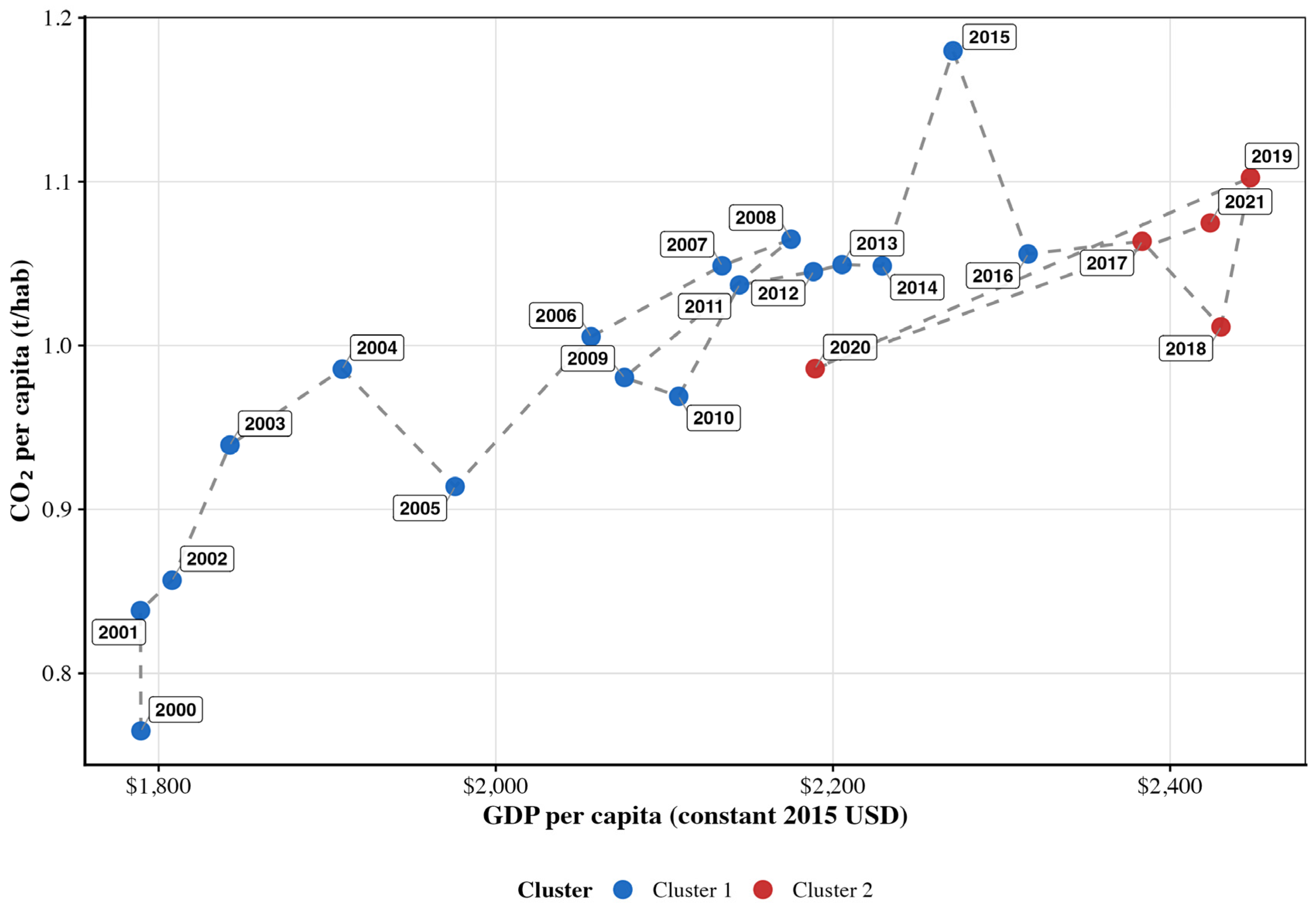
Figure 8 presents the structural development trajectory. GDP per capita versus CO₂ emissions per capita, classified by k-means cluster assignment (k = 2), Honduras 2000–2021. Each point represents one year, and the colours indicate the cluster assigned by k-means clustering. The trajectory reveals two clearly differentiated regimes. The analysis, based on verified primary data and a data-driven optimal-k procedure, identifies two statistically supported regimes.

3.3. Structural Breaks

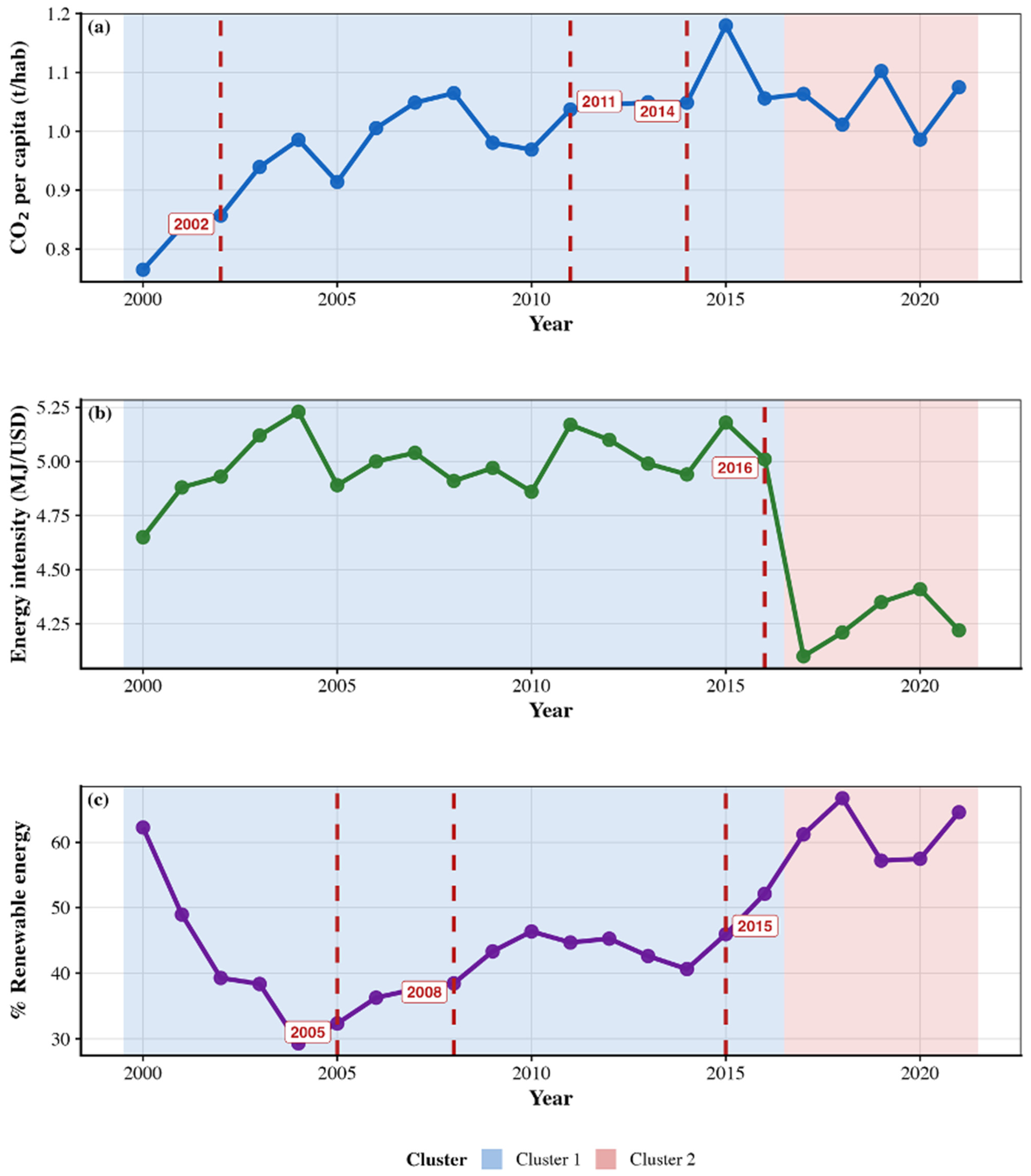
Figure 9 presents the structural break analysis obtained using the PELT algorithm for CO₂ emissions per capita, energy intensity, and renewable energy share. The PELT algorithm detected structural breaks in CO₂ emissions per capita in 2002, 2011, and 2014; in renewable energy share in 2005, 2008, and 2015; and a single break in energy intensity in 2016 (

Table 5. Structural breaks, Honduras 2000–2021.

Series	Detected Break Years	Number of Breaks
CO2 emissions per capita (t/capita)	2002, 2011, 2014	3
Renewable energy share (%)	2005, 2008, 2015	3
Energy intensity (MJ/USD)	2016	1

Note: PELT algorithm, (Panel B).

). These breakpoints provide an independent, model-based temporal signal that does not map neatly onto the two-cluster partition identified by k-means, suggesting that short-term volatility in the energy mix (captured by PELT) and the longer-run structural grouping (captured by k-means) reflect different, complementary aspects of the data.

3.4. Environmental Kuznets Curve

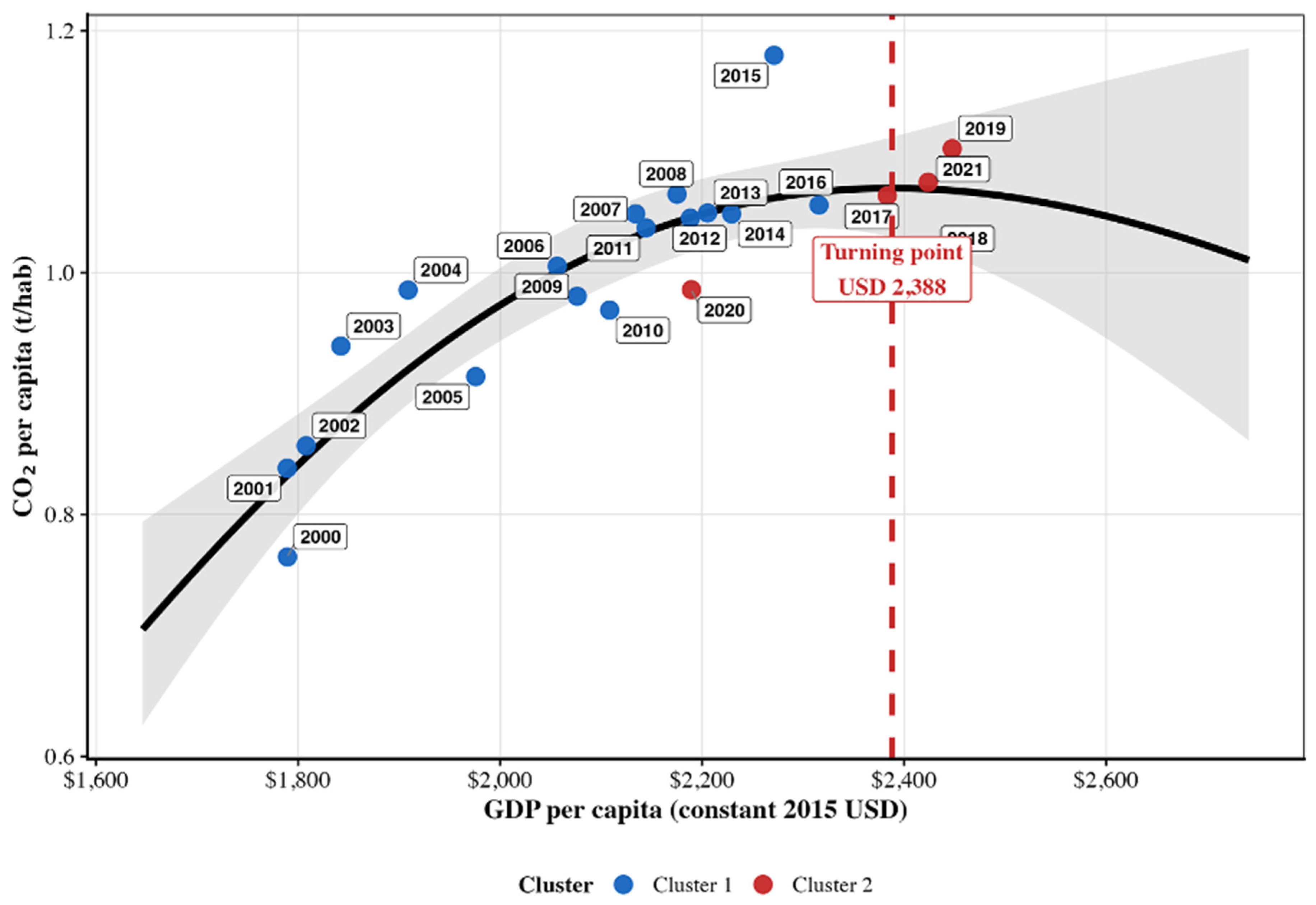
Figure 10 presents the fitted Environmental Kuznets Curve for Honduras during the estimated quadratic relationship between GDP per capita and CO₂ emissions per capita in Honduras, 2000–2021, with 95% confidence band and an estimated turning point. The estimated quadratic relationship between ln(GDP per capita) and ln(CO₂ emissions per capita) is consistent with an inverted-U pattern. As shown in

Table 6. OLS regression results for the EKC, Honduras 2000–2021 (Panel B).

Term	Coefficient (β)	Std. Error (OLS)	Std. Error (NW)	t-Value	p-Value	Sig.
Intercept (β0)	−182.167	63.186	44.368	−4.106	<0.001	***
ln(GDP pc)—β1	46.857	16.539	11.560	4.053	<0.001	***
[ln(GDP pc)]2—β2	−3.012	1.082	0.753	−4.000	<0.001	***
Adjusted R2	0.766	—	—	—	—	—
F-statistic	35.37 (df = 2, 19)	—	—	—	<0.001	***
EKC turning point	USD 2388 (2015 const.)	—	—	—	—	—
Durbin–Watson	1.947	—	—	—	0.290	no autocorrelation
Breusch–Pagan	1.145	—	—	—	0.564	n.s.

“—” indicates not applicable. n.s. = not significant (p ≥ 0.05). *** p < 0.001.

, the quadratic coefficient is negative and statistically significant (β₂ = −3.012, p < 0.001), while the linear coefficient is positive and significant (β₁ = 46.857, p < 0.001), jointly satisfying the EKC condition. The model explains a high proportion of the variance in emissions (adjusted R² = 0.766; F(2,19) = 35.37, p < 0.001). The estimated income turning point is USD 2388 per capita in constant 2015 prices (95% CI: USD 2156–2644, delta method [34]).

Diagnostic tests indicate no statistically significant serial autocorrelation (Durbin–Watson = 1.947, p = 0.290) and no statistically significant heteroscedasticity (Breusch–Pagan = 1.145, p = 0.564) in the OLS residuals. Newey–West standard errors, computed for robustness, are reported in Table 6 alongside the conventional OLS estimates; both yield identical significance conclusions given the absence of detected autocorrelation. Unit root tests (ADF lag = 1 and Phillips–Perron) [35,36] confirm that both ln(GDP per capita) and ln(CO₂ per capita) are integrated of order one, I(1). The Phillips–Perron test applied to the EKC regression residuals rejects the null of no cointegration at the 5% level (p = 0.022), supporting the levels-based OLS specification as an estimate of a long-run equilibrium relationship. This test uses the longer Panel A series (n = 34; see Section 2.2 and Table S1), which affords greater power than Panel B (n = 22) but for which the ADF test remains non-significant, reflecting limited power even at n = 34; cointegration evidence should be regarded as moderately supportive rather than conclusive. Full unit root and cointegration test results, including the KPSS stationarity test [37], are reported in Table S1 of the Supplementary Material. Dependent variable: ln(CO₂ per capita). NW = Newey–West corrected standard errors, reported for robustness; conclusions are unchanged given the absence of significant autocorrelation. *** p < 0.001. Conventional (non-robust) OLS standard errors are reported alongside the Newey–West standard errors for comparison; all three coefficients remain significant at the same level (p < 0.05) under both specifications, indicating that the Newey–West correction does not materially alter inference, consistent with the absence of detected autocorrelation.

Honduras’ GDP per capita was approximately USD 2527 in 2023, marginally exceeding the point estimate of USD 2388 (95% CI: USD 2156–2644) but remaining within the confidence interval; this comparison constitutes an out-of-sample extrapolation beyond the Panel B estimation window (maximum: USD 2448). This suggests that, descriptively, the country is located on the descending segment of the estimated EKC. However, this result should be interpreted cautiously: as shown in Section 3.5 and Section 3.6, this descriptive positioning relative to the EKC turning point does not, by itself, imply that income growth is the active mechanism driving any subsequent emissions decline, nor that renewable energy deployment is the temporal driver of such a decline. For this reason, the EKC result is interpreted together with the renewable energy, Granger causality, and Tapio decoupling findings. The EKC model above is estimated in levels by OLS, whereas the Granger causality tests in Section 3.5 use first-differenced series; this difference in specification is not contradictory but reflects the distinct purpose of each test. The cointegration evidence reported above (Phillips–Perron test on the EKC residuals, p = 0.022) supports treating the non-stationary GDP–CO₂ relationship in levels as a long-run equilibrium relationship, which justifies the levels-based EKC specification. The Granger tests, by contrast, require stationary series to satisfy the assumptions of the underlying vector autoregression and are therefore estimated in first differences, capturing short-run temporal precedence rather than the long-run relationship estimated by the EKC. An error-correction model (ECM), which would jointly estimate the long-run equilibrium and the short-run speed of adjustment within a single framework, is a natural extension for future work; the present study’s n = 34 annual observations are insufficient to estimate an ECM with adequate power, given the number of parameters such a specification requires, and this is noted as a direction for future research with longer or higher-frequency data.

3.5. Granger Temporal Precedence

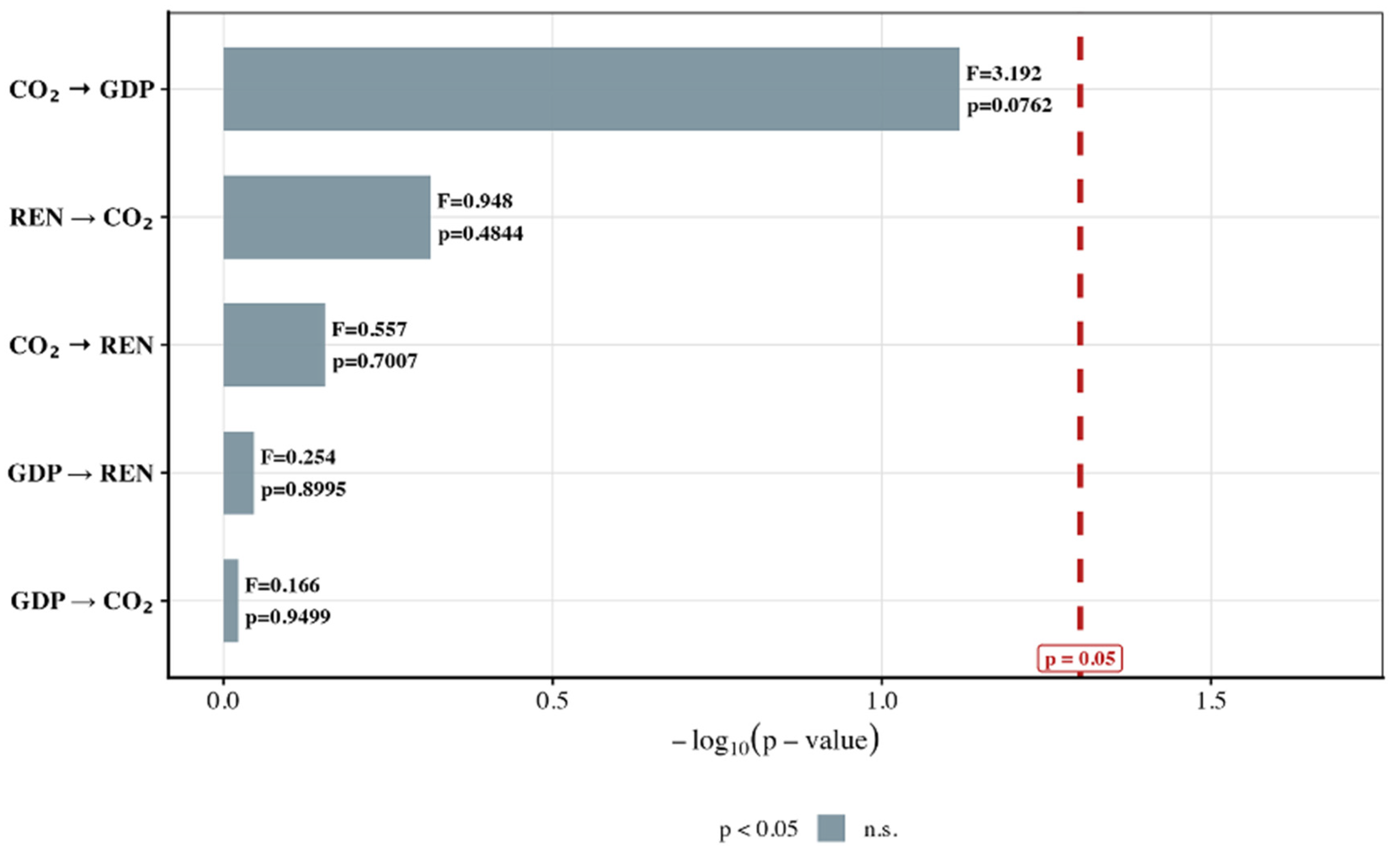
Figure 11 summarizes the Granger temporal precedence results. −log₁₀(p-value) representation of the five tested temporal relationships among GDP per capita, renewable energy share, and CO₂ emissions per capita, Honduras 2000–2021. The dashed line indicates the p = 0.05 significance threshold: no bar crosses it.

All variables were non-stationary in levels and were therefore first-differenced prior to testing. The Akaike Information Criterion, capped at a maximum lag of four to preserve degrees of freedom given n = 22, selected an optimal lag of four years.

Table 7. Granger causality test results, Honduras 2000–2021.

H0 (X Does Not Granger-Cause Y)	F-Statistic	p-Value	Conclusion
GDP pc does not cause CO2 pc	0.166	0.950	Do not reject H0
CO2 pc does not cause GDP pc	3.192	0.076	Do not reject H0 (marginal)
Renewables do not cause CO2 pc	0.948	0.484	Do not reject H0
CO2 pc does not cause renewables	0.557	0.701	Do not reject H0
GDP pc does not cause renewables	0.254	0.900	Do not reject H0

Note: first differences, optimal lag = 4 by AIC, capped given n = 22.

reports the five tested relationships.

None of the five tested relationships reached conventional statistical significance (α = 0.05). The strongest result, CO₂ per capita Granger-causing GDP per capita, approached but did not reach significance (F = 3.192, p = 0.076). Critically, renewable energy share did not show statistically significant temporal precedence over CO₂ emissions per capita (F = 0.948, p = 0.484), nor did GDP per capita (F = 0.166, p = 0.950). This result should be interpreted in light of the limited statistical power inherent to a 22-observation annual panel, and does not, by itself, rule out an economically meaningful relationship; rather, it indicates that the available data do not provide statistically robust evidence of temporal precedence in either direction.

These results should be interpreted with caution given the limited statistical power of Granger tests with n = 22 and up to four lags, which consume a substantial fraction of the available degrees of freedom. The non-significance of the renewable energy–emissions relationship reflects an absence of detectable temporal precedence in this short panel, not a theoretical claim that renewable energy deployment cannot reduce emissions.

3.6. Exploratory Machine-Learning Assessment

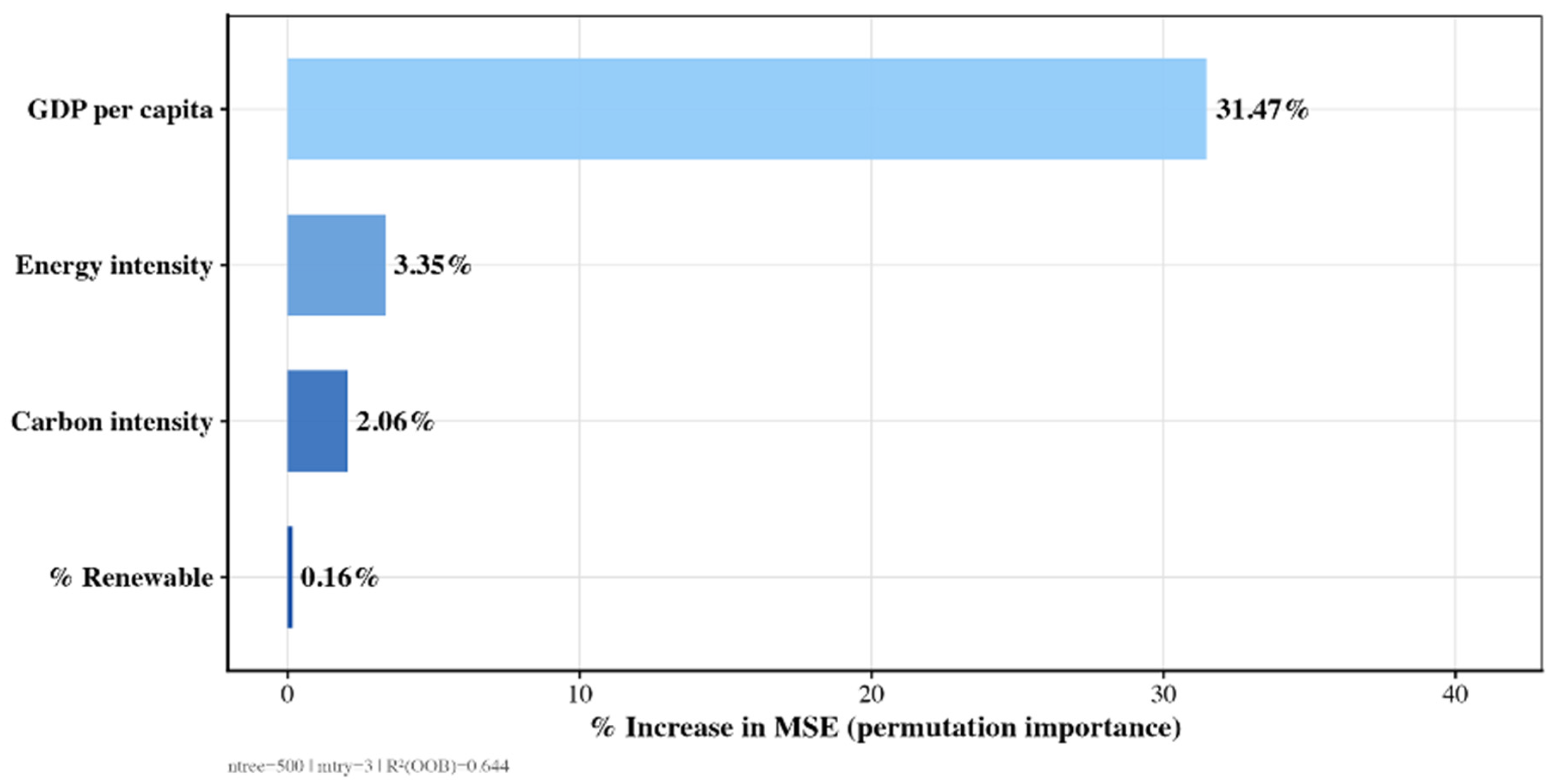
As an exploratory, descriptive complement to the econometric analyses, a Random Forest model was fitted on Panel B (n = 22) to assess the relative importance of the four explanatory variables. Given the small sample size, results should be interpreted as indicative of structural associations rather than as causal estimates or out-of-sample pre-dictions. Figure 12 presents the Random Forest variable importance results permutation-based importance (%IncMSE) of predictors used to estimate CO₂ emissions per capita, Honduras 2000–2021 (Panel B). The model achieved a moderate out-of-bag R² of 0.644 and an RMSE of 0.056 t CO₂/capita. Among the predictors, GDP per capita shows by far the highest permutation importance (%IncMSE = 31.47), followed by energy intensity (%IncMSE = 3.35), carbon intensity (%IncMSE = 2.06), and renewable energy share (%IncMSE = 0.16), as reported in

Table 8. Exploratory Random Forest variable importance, Honduras 2000–2021.

n	Rank	%IncMSE	IncNodePurity
GDP per capita	1st	31.47	0.124
Energy intensity	2nd	3.35	0.014
Carbon intensity	3rd	2.06	0.022
Renewable energy share	4th	0.16	0.008

. The Random Forest variable importance for prediction of CO₂ per capita, Honduras 2000–2021 (Panel B, n = 22). %IncMSE = percent increase in mean squared error when the variable is randomly permuted, normalized by its standard deviation across trees. ntree = 500; mtry = 3. R² (OOB) = 0.644; RMSE = 0.056. Results are exploratory given the small sample size.

These results indicate that GDP per capita is the dominant structural predictor of the level of CO₂ emissions, with renewable energy share contributing negligibly to predictive accuracy in this exploratory model. This finding is consistent with, and reinforces, the absence of statistically significant Granger causality from renewable energy share to emissions (Section 3.5): both the structural (Random Forest) and the temporal-precedence (Granger) analyses converge on the conclusion that income, not renewable energy deployment, is the variable most robustly associated with CO₂ emissions levels in this dataset. This contrasts with the hypothesis, common in parts of the decoupling literature, that renewable energy expansion is the proximate driver of emissions trajectories; in the Honduran case examined here, the data do not support that specific mechanism.

3.7. Tapio Decoupling Index

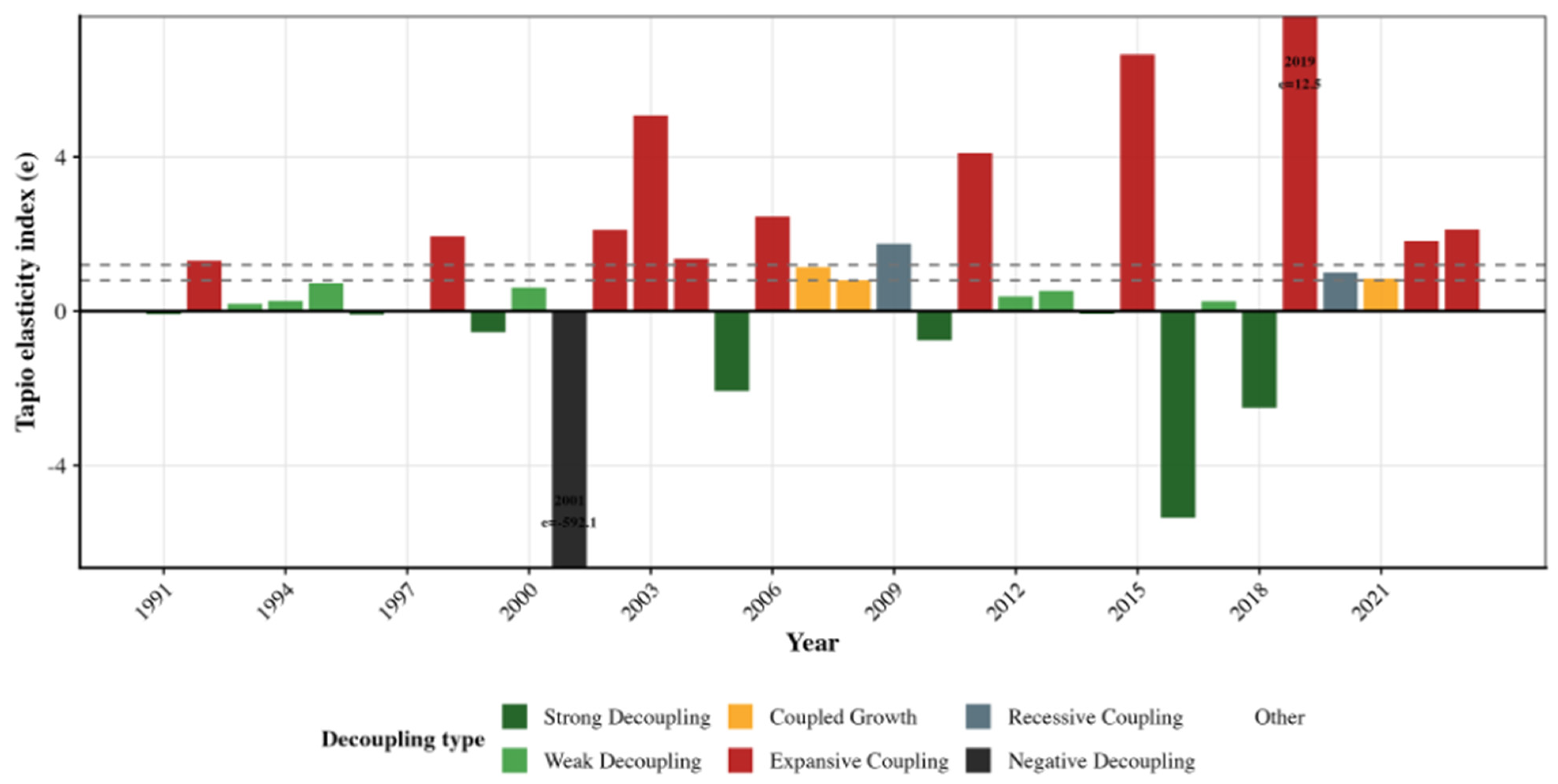
Figure 13 presents the annual Tapio decoupling elasticity index for 1991–2023. The annual Tapio elasticity index was calculated on Panel A (1990–2023, n = 33 annual transitions). Because the index divides the percentage change in CO₂ emissions by the percentage change in GDP, years in which GDP growth approached zero produce mathematically extreme elasticity values that do not reflect economically meaningful decoupling or coupling. This occurred most notably in 2001 (GDP growth ≈ −0.02%, yielding e ≈ −592.1) and, to a lesser extent, in 2019 (GDP growth ≈ 0.7%, yielding e ≈ 12.5). Both years are flagged explicitly in Figure 13 rather than allowed to distort the visual scale, and are excluded from the qualitative pattern description below; their underlying %ΔGDP and %ΔCO₂ values remain available in the full results table. Excluding these two flagged years, the annual classification shows a recurrent pattern of expansive coupling (e > 1.2) across multiple years scattered through the panel (e.g., 1992, 2002–2003, 2006, 2011, 2015, 2021–2023), interspersed with episodes of weak and strong decoupling (e.g., 1991, 1996–2000, 2005, 2010, 2014, 2017–2018) and isolated instances of recessive and coupled growth. No single multi-year period of sustained strong decoupling is evident in the annual series; rather, the year-to-year pattern is volatile, consistent with the absence of a statistically robust renewable-energy-driven decoupling signal identified in the Granger and Random Forest analyses (Section 3.5 and Section 3.6).

Table 9. Tapio (2005) [3] decoupling elasticity index by cluster and for the full period, Honduras.

Period	ΔGDP (%)	ΔCO2 (%)	Tapio e	Decoupling Type
Cluster 1 (2000–2016)	+29.41	+38.04	1.294	Expansive coupling
Cluster 2 (2017–2021)	+1.70	+1.05	0.621	Weak decoupling
Full period (1990–2023)	+451.83	+131.72	0.292	Weak decoupling

Note: Cluster period elasticities computed over Panel A using the first and last year within each cluster’s date range; the full-period elasticity uses 1990 and 2023 endpoints. Robustness check: CAGR-based elasticities (using compound annual growth rates) are 1.253 for Cluster 1 and 0.623 for Cluster 2, confirming identical Tapio classifications (expansive coupling and weak decoupling, respectively). Mean annual elasticities within each cluster (excluding flagged outlier years 2001 and 2019) are 1.168 (SD = 2.787) for Cluster 1 and −0.102 (SD = 1.632) for Cluster 2; the Cluster 2 mean is pulled toward zero by a COVID-related joint contraction in GDP and CO₂ in 2020, and the annual volatility in both clusters is documented in Figure 13.

reports the Tapio index aggregated by cluster and for the full 1990–2023 period. The apparent discrepancy between the frequency of annual expansive coupling episodes and the long-run weak decoupling result (e = 0.292) reflects the difference in temporal scale between the two metrics. Year-to-year elasticities are sensitive to supply-side shocks and macroeconomic volatility; the long-run aggregate elasticity averages across these fluctuations. The cumulative GDP and CO₂ growth differential—not the frequency of annual classifications—determines the long-run decoupling category. Cluster 1 (2000–2016) shows expansive coupling (e = 1.294: GDP grew 29.41% while CO₂ grew 38.04%). Cluster 2 (2017–2021) shows weak decoupling (e = 0.621: GDP grew 1.70% while CO₂ grew 1.05%), indicating that emissions grew more slowly than GDP, though not in absolute terms. Over the full 1990–2023 period, GDP per capita grew 451.83% while CO₂ per capita grew 131.72%, yielding an aggregate elasticity of e = 0.292, classified as weak decoupling over the long run.

A departmental eco-efficiency exercise was also conducted using estimated, non-official departmental GDP shares. Because these shares cannot be attributed to an official source, the full exercise—including the departmental map, the underlying proxy construction, and a sensitivity analysis under alternative share assumptions—is presented in the Supplementary Material (Figure S1 and Table S3) rather than as a main-text result.

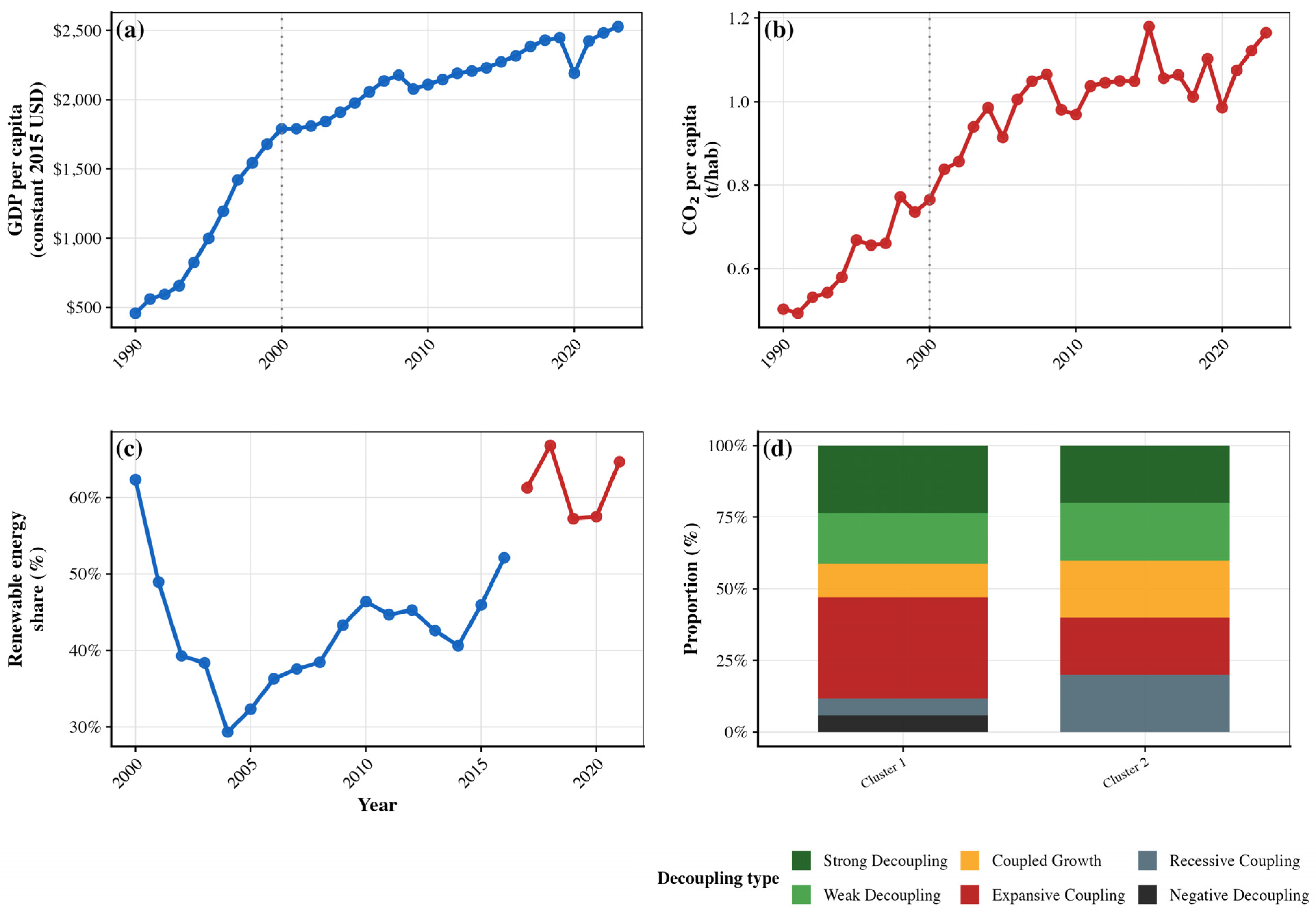
An integrated dashboard (Figure 14) summarizes the four key annual series and the cluster-level Tapio composition in a single visual synthesis, consolidating the descriptive trends (Section 3.1) and the decoupling classification (Section 3.7) for ease of reference. Honduras 1990–2023. Panel (a): GDP per capita (Panel A series, 1990–2023). Panel (b): CO₂ per capita (Panel A series, 1990–2023). Panel (c): renewable energy share (Panel B series, 2000–2021). Panel (d): percentage composition of annual Tapio decoupling classifications by k-means cluster (Cluster 1, 2000–2016; Cluster 2, 2017–2021). Panels (a) and (b) reproduce the series shown in Figure 5; panel (d) presents, in proportional form, the same annual classifications underlying Table 9 and Figure 13.

4. Discussion

The k-means results identify two, statistically supported structural regimes. This indicates that the energy–economy system has undergone meaningful structural change.

Cluster 1 (2000–2016) is characterized by lower renewable energy share (42.6%) and higher energy intensity (4.99 MJ/USD), while Cluster 2 (2017–2021) shows higher renewable energy share (61.5%) and lower energy intensity (4.26 MJ/USD), broadly consistent with the documented expansion of solar photovoltaic and wind generation in Honduras following the 2007 regulatory framework and subsequent project commissioning from 2013 onward [5,6,7]. The PELT-detected structural breaks (2002, 2005, 2008, 2011, 2014, 2015, 2016) do not map cleanly onto this two-cluster boundary, suggesting that shorter-term volatility in specific indicators (particularly renewable share and CO₂ per capita) and the longer-run structural grouping captured by clustering reflect different, complementary temporal scales of change rather than a single, sharply demarcated transition.

This two-to-three-year lag between the last PELT-detected break in CO₂ per capita (2014) and the k-means cluster boundary (2016/2017) is plausibly substantive rather than merely a methodological artefact. PELT identifies the point at which the mean and variance of a single series shift, which can register the initial effect of a specific policy or investment decision (e.g., the commissioning of individual renewable projects) as soon as it measurably alters the emissions series. Clustering, by contrast, groups years by their joint position across all four variables simultaneously, and will only reassign a year once renewable share, energy intensity, and the GDP–CO₂ relationship have jointly moved enough to dominate the multivariate distance metric. A 2–3-year gap is therefore consistent with a delay between the initial regulatory or investment decision and its full diffusion into system-wide energy intensity and renewable share, rather than indicating that the two methods are simply responding to noise. This interpretation is necessarily descriptive, since the annual panel is too short to formally test the mechanism.

The EKC results provide robust statistical support for an inverted-U relationship between GDP per capita and CO₂ emissions per capita (β₂ = −3.012, p < 0.001; adjusted R² = 0.766), with an estimated turning point of USD 2388 per capita (95% CI: USD 2156–2644, delta method). Honduras’ 2023 GDP per capita (USD 2527, Panel A) marginally exceeds the point estimate but falls within the 95% confidence interval, and this comparison constitutes an out-of-sample extrapolation beyond Panel B’s estimation window (maximum: USD 2448. Unlike in some prior illustrative analyses, the Durbin–Watson statistic here indicates no significant serial autocorrelation (DW = 1.947, p = 0.290), strengthening confidence in the validity of the standard errors underlying this result.

This levels-based EKC specification rests on the assumption that ln(GDP per capita) and ln(CO₂ per capita) are cointegrated; as reported in Section 3.4, this assumption receives only mixed support—the Phillips–Perron test on the regression residuals rejects the null of no cointegration (p = 0.022), but the ADF test on the same residuals does not (p = 0.188). Because this evidence is moderately rather than conclusively supportive, both the quadratic coefficient (β₂ = −3.012) and the derived turning point (USD 2388) should be read as consistent with, rather than definitively established by, a stable long-run equilibrium relationship. If the true data-generating process were instead a spurious levels regression, the standard errors reported in Table 6—already conservative given the Newey–West correction—could still understate the true uncertainty, and the turning point’s 95% confidence interval (USD 2156–2644) should accordingly be treated as a lower bound on the true estimation uncertainty rather than a complete accounting of it. This caveat does not overturn the EKC finding, since the Phillips–Perron test, generally preferred for short samples, does support cointegration, but it is a material qualification that should temper how confidently the turning point is used as a basis for policy inference.

However, descriptively crossing an EKC turning point is not equivalent to demonstrating that income growth is the active mechanism reducing emissions, nor that this positioning will translate into sustained absolute decoupling; the EKC is, at most, a necessary but not sufficient condition, and the temporal-precedence evidence presented below argues for caution in attributing any future emissions decline to income growth per se.

The Granger causality results are, in this respect, the most consequential. None of the five tested temporal relationships, including renewable energy share Granger-causing CO₂ emissions, reached statistical significance at conventional levels (all p > 0.05). This directly contradicts the renewable-energy-driven decoupling narrative that might otherwise be inferred from the EKC result alone, and underscores the methodological point raised by Zilio and Caraballo [19] that EKC evidence for Latin America should be interpreted cautiously and triangulated against other indicators. The absence of significant Granger causality should not, however, be over-interpreted as proof that no causal relationship exists; with n = 22 and first-differenced series, the statistical power of these tests is limited, and a Type II error (failing to detect a real but modest effect) cannot be ruled out. The appropriate interpretation is that the available data do not provide statistically robust evidence for temporal precedence in either direction, which is itself an informative and policy-relevant finding.

The Random Forest results corroborate and extend this picture. GDP per capita is overwhelmingly the dominant predictor of CO₂ emissions levels (%IncMSE = 31.47), while renewable energy share contributes negligibly (%IncMSE = 0.16) to out-of-sample predictive accuracy. Read alongside the Granger results, this suggests that income is both the structural determinant of emissions levels and shows no detected temporal precedence effect from renewable deployment on emissions changes, a combination that, taken together, offers little statistical support for the proposition that Honduras’ renewable energy expansion has, to date, been the proximate driver of any emissions moderation. This is an important corrective to narratives, common in policy and some academic discourse, that treat renewable energy capacity expansion as automatically equivalent to decoupling; the present evidence for Honduras does not support that equivalence.

The co-existence of an estimated EKC turning point and the absence of a renewable-energy-driven decoupling signal reflects two distinct mechanisms. The EKC captures income-driven structural change in the aggregate GDP–CO₂ relationship: as per capita income has grown, the emissions intensity of growth has declined—an income effect. The Granger and Random Forest analyses address whether the timing and scale of renewable deployment adds independent information about emissions, conditional on income. The absence of a significant signal is consistent with Honduras’ renewable expansion being dominated by large hydropower subject to hydrological variability, and intermittent capacity that does not generate a detectable monotonic emissions-displacement trajectory over a 22-year annual panel.

The annual Tapio index reinforces this more cautious reading. Once the two mathematically extreme years (2001 and 2019, driven by near-zero GDP growth denominators) are appropriately flagged rather than allowed to distort the analysis, the annual elasticity series shows a volatile, non-monotonic pattern with recurrent episodes of expansive coupling interspersed with weak and strong decoupling, rather than a clear secular trend toward decoupling. Cluster 2 (2017–2021) registers weak decoupling (e = 0.621), and the full 1990–2023 period registers weak decoupling overall (e = 0.292); a meaningfully different and more modest characterization than a narrative of strong, renewable-driven decoupling would suggest.

This classification for Cluster 2, however, warrants a specific caveat. The period comprises only five annual observations, one of which—2020—reflects an exogenous COVID-19 shock that produced a simultaneous contraction in both GDP and CO₂ emissions, qualitatively distinct from the endogenous energy-system transition that clustering is designed to capture. As a sensitivity check, we recomputed the elasticity using only the pre-pandemic sub-trend (2017–2019): GDP grew 2.70% and CO₂ grew 3.66%, yielding e = 1.357—expansive coupling, the opposite classification from the e = 0.621 (weak decoupling) obtained using the full 2017–2021 endpoints (Supplementary Table S4). Cluster 2’s decoupling classification is therefore highly sensitive to the inclusion of the pandemic year and should be treated as provisional rather than as evidence of a stable structural tendency. This sensitivity does not affect the study’s central full-period conclusion (weak decoupling, e = 0.292, 1990–2023), which averages across 34 years and is not driven by any single anomalous observation.

The spatial eco-efficiency exercise (Supplementary Figure S1 and Table S3), presented as an explicitly exploratory illustration given the absence of official departmental statistics, is consistent with the well-documented concentration of Honduran economic activity in Cortés and Francisco Morazán. This concentration implies that any future climate and energy policy aimed at improving eco-efficiency should consider territorial differentiation, though confirming this quantitatively requires official subnational GDP and emissions data that are not currently available.

Overall, the findings indicate that Honduras has likely crossed the EKC income turning point, and that its electricity mix has diversified toward renewable sources, particularly from the mid-2010s onward. However, the statistical evidence assembled here, specifically, the absence of significant Granger causality from renewable energy share to emissions, the overwhelming dominance of GDP per capita as a Random Forest predictor, and the volatile rather than monotonically improving annual Tapio series, does not support a confident claim that renewable energy deployment has, to date, produced robust, sustained decoupling in Honduras. This is a more conservative conclusion than might be drawn from the EKC result in isolation, and it illustrates the methodological value of triangulating multiple, complementary empirical approaches rather than relying on any single test.

This study also has limitations beyond those already noted. First, the complete four-variable panel is limited to 22 annual observations, substantially restricting the statistical power of the EKC, Granger, and Random Forest analyses; results from these methods should be regarded as indicative rather than conclusive, and replication with longer or higher-frequency series is strongly encouraged as data become available. Second, Granger causality identifies temporal precedence, not structural or counterfactual causality; failure to reject the null hypothesis does not establish the absence of a causal relationship. Third, Random Forest results are explicitly exploratory given the small sample. Fourth, the departmental eco-efficiency results rely on estimated proxies and must be validated using official subnational GDP and emissions inventories once available. Despite these limitations, the triangulation of clustering, structural breaks, EKC modelling, Granger tests, machine learning, and Tapio classification, each method’s strengths compensating for another’s weaknesses, provides a methodologically transparent and statistically grounded basis for assessing Honduras’ low-carbon development trajectory.

5. Conclusions

This study assessed whether Honduras has decoupled economic growth from CO₂ emissions during 1990–2023, using verified primary data from the World Bank and the Global Carbon Project and integrating k-means clustering, PELT structural break detection, EKC modelling, Granger temporal precedence tests, Random Forest analysis, and the Tapio decoupling index. Because complete four-variable coverage is available only from 2000 onward, the analysis explicitly distinguishes a 34-year GDP–CO₂ series from a 22-year complete panel used for the multivariate analyses, avoiding both data imputation and silent exclusion of incomplete years.

The main empirical findings are fourfold. First, cluster analysis identifies two statistically preferred structural regimes (2000–2016 and 2017–2021), reflecting lower renewable energy share and higher energy intensity in the earlier regime and the reverse pattern in the more recent one. Second, the Environmental Kuznets Curve hypothesis is empirically supported (β₂ = −3.012, p < 0.001; adjusted R² = 0.766), with an estimated turning point of USD 2388 per capita (95% CI: USD 2156–2644), which Honduras’ 2023 GDP per capita marginally exceeds as an out-of-sample extrapolation. Third, Granger causality tests find no statistically significant temporal precedence in either direction between GDP per capita, renewable energy share, and CO₂ emissions per capita (all p > 0.05), and Random Forest analysis confirms that GDP per capita (%IncMSE = 31.47) vastly outweighs renewable energy share (%IncMSE = 0.16) as a predictor of emissions levels. Fourth, the annual Tapio index reveals a volatile rather than monotonically improving decoupling pattern, with the full 1990–2023 period classified as weak decoupling (e = 0.292).

Taken together, these results indicate that while Honduras has likely surpassed the EKC income threshold and has diversified its electricity mix toward renewable sources, the available statistical evidence does not support a confident narrative that renewable energy expansion has been the proximate, temporally precedent driver of emissions moderation. GDP per capita remains the dominant structural determinant of emissions levels.

From a policy perspective, these findings require a stratified response that distinguishes between income-related decoupling mechanisms and the limited statistical evidence of renewable-driven emissions reduction. The specific instruments proposed below extend beyond what this study’s econometric and machine-learning results can directly test: only the general direction implied by the two central findings—that income-driven structural change appears underway, and that renewable capacity expansion alone has not been shown to drive an emissions reduction—follows from the results themselves. The specific instruments (time-of-use tariffs, electric-vehicle incentives, minimum energy performance standards) are grounded in the broader energy-policy literature rather than in this paper’s own estimates, and are presented as the authors’ policy judgement about how those two findings could be operationalized, not as conclusions that follow mechanically from the empirical analysis. The EKC result suggests that Honduras may be entering a stage in which economic growth can be accompanied by lower emissions intensity, but this outcome should not be interpreted as automatic. To prevent rebound effects, policy should prioritize end-use energy efficiency, demand-side management, and sector-specific standards. In the residential and commercial sectors, visible energy-efficiency labels for high-consumption equipment, particularly air-conditioning systems, should be strengthened because cooling demand is a major electricity load in warm regions of the country. Time-of-use tariffs, which are a widely documented instrument in developing-country electricity systems [38] and have been found in a survey of 15 experiments to reduce residential peak demand by roughly 3–6% [39], should also be evaluated as a promising instrument to shift consumption away from peak periods, reduce system stress, and support more efficient electricity use.

The absence of a robust renewable-energy-driven decoupling signal implies that renewable capacity expansion alone is insufficient. Renewable generation should be coupled with grid integration measures, electricity-loss reduction, battery storage, flexible demand, and electrification of final uses that currently depend on fossil fuels. In the transport sector, which represents the largest final energy use, policy should combine short-term measures such as eco-driving programmes with medium- and long-term incentives for hybrid and electric vehicles, renewable-powered charging infrastructure, and battery-supported charging systems. This would allow renewable electricity to displace oil consumption rather than merely increase installed capacity.

In the industrial sector, policy should move beyond regulation alone. Although Minimum Energy Performance Standards for electric motors have been established, their effectiveness will depend on implementation, enforcement, and economic incentives for replacing inefficient motor systems. Government-supported replacement programmes, concessional financing, or fiscal incentives for high-efficiency motors would help reduce electricity demand, improve industrial competitiveness, and reinforce the emissions-intensity reductions suggested by the EKC result. Overall, the evidence indicates that Honduras’ low-carbon strategy should not rely only on renewable electricity expansion, but on an integrated package of renewable energy, energy efficiency, transport electrification, tariff reform, and targeted end-use policies.

The study also highlights the importance of territorial differentiation and of further methodological work. The exploratory spatial eco-efficiency results, based on estimated proxies, suggest that national decoupling patterns are unlikely to be evenly distributed across departments, reinforcing the need for official subnational energy and emissions data. Future research should prioritize the construction of longer, higher-frequency, and sub nationally disaggregated datasets for Honduras and other Central American economies, both to confirm or revise the present findings and to support increasingly granular, evidence-based climate governance.

References

1. World Commission on Environment and Development. Our Common Future; Oxford University Press: Oxford, UK, 1987. [Google Scholar]
2. Intergovernmental Panel on Climate Change. Climate Change 2022: Mitigation of Climate Change. Contribution of Working Group III to the Sixth Assessment Report of the Intergovernmental Panel on Climate Change; Shukla, P.R., Skea, J., Slade, R., Al Khourdajie, A., van Diemen, R., McCollum, D., Pathak, M., Some, S., Vyas, P., Fradera, R., et al., Eds.; Cambridge University Press: Cambridge, UK; New York, NY, USA, 2022. [Google Scholar] [CrossRef] [Scilit]
3. Tapio, P. Towards a Theory of Decoupling: Degrees of Decoupling in the EU and the Case of Road Traffic in Finland between 1970 and 2001. Transp. Policy 2005, 12, 137–151. [Google Scholar] [CrossRef] [Scilit]
4. Tong, K.; Sun, S. Multi-Dimensional Decoupling Analysis in the Context of Energy Use: Dynamic Well-Being, Resource, and Impact Decoupling Relationships in China. Appl. Energy 2024, 359, 122726. [Google Scholar] [CrossRef] [Scilit]
5. Ramos-Gómez, J.I.; Molina-García, A.; Muñoz-Tabora, J. Power System Modeling and Simulation for Distributed Generation Integration: Honduras Power System as a Case Study. Energies 2025, 18, 4777. [Google Scholar] [CrossRef] [Scilit]
6. Tome-Amador, D.; Varela-Aguilera, C.; Rivera-López, D.A.; Muñoz Tabora, J. Application of Battery and Flywheel Energy Storage Systems for Frequency Regulation in the Honduran Power Grid. Energies 2025, 18, 6287. [Google Scholar] [CrossRef] [Scilit]
7. Fajardo, A.R.; Martinez, M.L.; Tabora, J.M.; Huaquisaca, J.C.; Rivera, D.A. Hosting Capacity: A Systematic Review from an Honduran Perspective. In Proceedings of the 2025 16th IEEE International Conference on Industry Applications (INDUSCON), São Sebastião, Brazil, 14–17 October 2025; pp. 1–8. [Google Scholar]
8. Flores, W.C.; Ojeda, O.A.; Flores, M.A.; Rivas, F.R. Sustainable Energy Policy in Honduras: Diagnosis and Challenges. Energy Policy 2011, 39, 551–562. [Google Scholar] [CrossRef] [Scilit]
9. Flores, W.C. Honduras’ Energy Policy: Post Coup d’état Energy Scenarios. Lat. Am. Policy 2018, 9, 331–348. [Google Scholar] [CrossRef] [Scilit]
10. Grossman, G.M.; Krueger, A.B. Environmental Impacts of a North American Free Trade Agreement; NBER Working Paper No. 3914; National Bureau of Economic Research, Inc.: Cambridge, MA, USA, 1991. [Google Scholar] [CrossRef] [Scilit]
11. Grossman, G.M.; Krueger, A.B. Economic Growth and the Environment. Q. J. Econ. 1995, 110, 353–377. [Google Scholar] [CrossRef] [Scilit]
12. Panayotou, T. Empirical Tests and Policy Analysis of Environmental Degradation at Different Stages of Economic Development; International Labour Organization: Geneva, Switzerland, 1993. [Google Scholar]
13. Stern, D.I. Environmental Kuznets Curve. In Encyclopedia of Energy; Cleveland, C.J., Ed.; Elsevier: Amsterdam, The Netherlands, 2004; Volume 2, pp. 517–525. [Google Scholar] [CrossRef] [Scilit]
14. Dinda, S. Environmental Kuznets Curve Hypothesis: A Survey. Ecol. Econ. 2004, 49, 431–455. [Google Scholar] [CrossRef] [Scilit]
15. Jordan, M.I.; Mitchell, T.M. Machine Learning: Trends, Perspectives, and Prospects. Science 2015, 349, 255–260. [Google Scholar] [CrossRef] [Scilit] [PubMed]
16. Killick, R.; Fearnhead, P.; Eckley, I.A. Optimal Detection of Changepoints with a Linear Computational Cost. J. Am. Stat. Assoc. 2012, 107, 1590–1598. [Google Scholar] [CrossRef] [Scilit]
17. Hao, Y.; Huang, Z.; Wu, H. Do Carbon Emissions and Economic Growth Decouple in China? An Empirical Analysis Based on Provincial Panel Data. Energies 2019, 12, 2411. [Google Scholar] [CrossRef] [Scilit]
18. Al-mulali, U.; Tang, C.F.; Ozturk, I. Estimating the Environment Kuznets Curve Hypothesis: Evidence from Latin America and the Caribbean Countries. Renew. Sustain. Energy Rev. 2015, 50, 918–924. [Google Scholar] [CrossRef] [Scilit]
19. Zilio, M.; Caraballo, M.Á.; Zilio, M.; Caraballo, M.Á. ¿El final de la curva de Kuznets de carbono? Un análisis semiparamétrico para la América Latina y el Caribe. EL Trimest. Económico 2014, 81, 241–270. [Google Scholar] [CrossRef] [Scilit]
20. Tabora, J.M.; Paixão Júnior, U.C.; Rodrigues, C.E.M.; Bezerra, U.H.; Tostes, M.E.d.L.; Albuquerque, B.S.d.; Matos, E.O.d.; Nascimento, A.A.d. Hybrid System Assessment in On-Grid and Off-Grid Conditions: A Technical and Economical Approach. Energies 2021, 14, 5284. [Google Scholar] [CrossRef] [Scilit]
21. Akram, R.; Chen, F.; Khalid, F.; Ye, Z.; Majeed, M.T. Heterogeneous Effects of Energy Efficiency and Renewable Energy on Carbon Emissions: Evidence from Developing Countries. J. Clean. Prod. 2020, 247, 119122. [Google Scholar] [CrossRef] [Scilit]
22. Yao, S.; Zhang, S.; Zhang, X. Renewable Energy, Carbon Emission and Economic Growth: A Revised Environmental Kuznets Curve Perspective. J. Clean. Prod. 2019, 235, 1338–1352. [Google Scholar] [CrossRef] [Scilit]
23. Ahmed, M.M.; Shimada, K. The Effect of Renewable Energy Consumption on Sustainable Economic Development: Evidence from Emerging and Developing Economies. Energies 2019, 12, 2954. [Google Scholar] [CrossRef] [Scilit]
24. Shahbaz, M.; Mahalik, M.K.; Shah, S.H.; Sato, J.R. Time-Varying Analysis of CO2 Emissions, Energy Consumption, and Economic Growth Nexus: Statistical Experience in next 11 Countries. Energy Policy 2016, 98, 33–48. [Google Scholar] [CrossRef] [Scilit]
25. Leiva, B.; Rubio-Varas, M. The Energy and Gross Domestic Product Causality Nexus in Latin America 1900–2010. Int. J. Energy Econ. Policy 2020, 10, 423–435. [Google Scholar] [CrossRef] [Scilit]
26. Sarmiento, C.R.A.; Heller, J.J.P. VAR Model Analysis of Energy Consumption, CO2 Emissions, Financial Development, and Economic Growth in Honduras (1980–2022). In Proceedings of the 23rd LACCEI International Multi-Conference for Engineering, Education and Technology (LACCEI): “Engineering, Artificial Intelligence, and Sustainable Technologies in Service of Society”; LACCEI: Boca Raton, FL, USA, 2025. [Google Scholar] [CrossRef] [Scilit]
27. Flores, W.C.; Pineda, G.M. Social Inclusion in Energy Regulation of Honduras: A Necessary Analysis. In Proceedings of the 2022 IEEE Biennial Congress of Argentina (ARGENCON), San Juan, Argentina, 7–9 September 2022; pp. 1–5. [Google Scholar]
28. Pineda-Guzman, R.; Acevedo Alvarado, P.S.; Sánchez-Pérez, P.A.; Castellanos, S. Pathways to Decarbonize Honduras’ Power Sector. Environ. Sci. Technol. 2025, 59, 4409–4417. [Google Scholar] [CrossRef] [Scilit] [PubMed]
29. World Bank. World Development Indicators; The World Bank Group: Washington, DC, USA. Available online: https://databank.worldbank.org/source/world-development-indicators (accessed on 20 June 2026).
30. Global Carbon Budget (2025); Population Based on Various Sources (2024)—With Major Processing by Our World in Data. “CO2 Emissions per Capita” [Dataset]. Global Carbon Project, “Global Carbon Budget V15”; Various Sources, “Population” [Original Data]. Available online: https://ourworldindata.org/grapher/co-emissions-per-capita (accessed on 20 June 2026).
31. Kaufman, L.; Rousseeuw, P.J. Finding Groups in Data: An Introduction to Cluster Analysis; John Wiley & Sons: Hoboken, NJ, USA, 1990. [Google Scholar]
32. Breiman, L. Random Forests. Mach. Learn. 2001, 45, 5–32. [Google Scholar] [CrossRef] [Scilit]
33. Kuhn, M. Building Predictive Models in R Using the Caret Package. J. Stat. Softw. 2008, 28, 1–26. [Google Scholar] [CrossRef] [Scilit]
34. Oehlert, G.W. A Note on the Delta Method. Am. Stat. 1992, 46, 27–29. [Google Scholar] [CrossRef] [Scilit]
35. Dickey, D.A.; Fuller, W.A. Distribution of the Estimators for Autoregressive Time Series with a Unit Root. J. Am. Stat. Assoc. 1979, 74, 427–431. [Google Scholar] [CrossRef] [Scilit]
36. Phillips, P.C.B.; Perron, P. Testing for a Unit Root in Time Series Regression. Biometrika 1988, 75, 335–346. [Google Scholar] [CrossRef]
37. Kwiatkowski, D.; Phillips, P.C.B.; Schmidt, P.; Shin, Y. Testing the Null Hypothesis of Stationarity against the Alternative of a Unit Root. J. Econom. 1992, 54, 159–178. [Google Scholar] [CrossRef] [Scilit]
38. World Bank. Falling Short: A Global Survey of Electricity Tariff Design; World Bank: Washington, DC, USA, 2020. [Google Scholar]
39. Faruqui, A.; Sergici, S. Household Response to Dynamic Pricing of Electricity: A Survey of 15 Experiments. J. Regul. Econ. 2010, 38, 193–225. [Google Scholar] [CrossRef] [Scilit]
Figure 1. Bibliometric keyword mapping: (a) main thematic clusters; (b) temporal evolution of keywords in the reviewed literature.
Sustainability 18 07726 g001
Figure 2. Annual publications by country. Stacked annual distribution of publications for the top 15 contributing countries from 2010 to 2025.
Sustainability 18 07726 g002
Figure 3. Regional and document-type distribution. (a) Latin American publication distribution by country; numbers indicate the count of publications per country on the color scale shown in the legend (1–3). (b) Document-type composition of the reviewed literature.
Sustainability 18 07726 g003
Figure 4. Methodological workflow used to assess the economic growth–CO2 emissions decoupling trajectory in Honduras. Descriptive steps use the full 1990–2023 GDP-CO2 series (Panel A, n = 34); steps 3.1–3.6 use the complete four-variable panel (Panel B, 2000–2021, n = 22).
Sustainability 18 07726 g004
Figure 5. Long-run series of GDP per capita and CO2 emissions per capita, Honduras, 1990–2023 (Panel A). Red: CO2 per capita; blue: GDP per capita. The grey dotted vertical line marks the year 2000, the start of Panel B coverage. Source: Own elaboration. Data from [29,30].
Sustainability 18 07726 g005
Figure 6. Complete four-variable panel, Honduras, 2000–2021 (Panel B). Each panel is labeled with its variable (purple: renewable energy share; red: CO2 per capita; green: energy intensity; blue: GDP per capita). Source: Own elaboration. Data from [29,30].
Sustainability 18 07726 g006
Figure 7. Optimal number of clusters, Honduras 2000–2021 (Panel B, n = 22). (a) Elbow plot (total within-cluster sum of squares); (b) average silhouette width. The red dashed line marks the selected k = 2.
Sustainability 18 07726 g007
Figure 8. Structural development trajectory, Honduras 2000–2021. Source: Own elaboration. Data from [29,30].
Sustainability 18 07726 g008
Figure 9. Structural break analysis. PELT-detected breakpoints in CO2 emissions per capita, renewable energy share, and energy intensity, Honduras 2000–2021 (Panel B). (a) CO2 per capita; (b) energy intensity; (c) renewable energy share. Red dashed vertical lines mark PELT-detected breakpoints (labeled by year); shaded bands indicate the k-means Cluster 1/Cluster 2 regimes (see legend).
Sustainability 18 07726 g009
Figure 10. Environmental Kuznets Curve. Blue points: Cluster 1 (2000–2016); red points: Cluster 2 (2017–2021); black curve: fitted quadratic EKC; grey band: 95% confidence interval; red dashed line: estimated turning point (USD 2388). Source: Own elaboration. Data from [29,30].
Sustainability 18 07726 g010
Figure 11. Granger temporal precedence results.
Sustainability 18 07726 g011
Figure 12. Random Forest variable importance. Permutation-based importance of predictors used to estimate CO2 emissions per capita.
Sustainability 18 07726 g012
Figure 13. Annual Tapio decoupling elasticity index, Honduras 1991–2023 (Panel A). Bar color indicates the decoupling type classification for that year (see legend); grey dashed horizontal lines mark the elasticity thresholds (e = 0.8 and e = 1.2) used to classify decoupling types.
Sustainability 18 07726 g013
Figure 14. Integrated summary dashboard, Honduras 1990–2023. (a) GDP per capita; (b) CO2 per capita; (c) renewable energy share; (d) proportion of years by decoupling type, by cluster (see legend). The grey dotted vertical line in (a,b) marks the year 2000.
Sustainability 18 07726 g014