Demand Hidden by Stockouts: Censored Demand Recovery and Green Waste-Reduction Forecasting for Sustainable Fresh-Food Consumption Under Emerging-Market Urbanization

Abstract

Fresh-food retail demand is only partially observed when products stock out: point-of-sale records report sales, whereas the unmet part of demand is censored. This study develops a probabilistic decision-support framework, termed CADRE, that treats stockout-flagged observations as lower bounds, separates recurring diurnal structure from censoring effects, and shapes the replenishment decision with an asymmetric shortage–spoilage loss. The evaluation uses FreshRetailNet-50K, an hourly Chinese fresh-retail benchmark with observed stockout labels, and a complementary daily robustness experiment on the Ecuadorian Favorita panel with a constructed high-demand censoring mask. On FreshRetailNet-50K, CADRE reduces weighted absolute percentage error (WAPE) from 39.42% for the TimeXer backbone to 36.71% and reduces re-censored demand bias from $-8.1\%$ to $-1.3\%$. In a controlled replenishment simulation on known re-censored demand, modelled waste decreases from 9.8% under a censored-sales policy to 6.4% under CADRE while service level increases from 92.9% to 94.7%. These results indicate potential improvements in replenishment decision support under the evaluated assumptions, rather than measured operational food-waste or emissions reductions. Operational food-waste and emission effects remain to be validated through field deployment.

1. Introduction

Sustainability in fresh-food retail is usually framed as a balancing act. Order generously and unsold produce is thrown away; order cautiously and shelves sit empty, sales are lost, and shoppers leave disappointed. Because waste and availability seem to pull in opposite directions, a manager who sets out to cut waste expects to pay for it in service, and one who wants full shelves expects to pay in spoilage. The stakes are not modest. Roughly a fifth of the food available to consumers is wasted, and food loss and waste together account for 8 to 10 percent of global greenhouse-gas emissions [1,2]. In fast-urbanizing emerging markets, where modern grocery chains are spreading quickly and per-capita household waste already rivals that of richer economies, the retail ordering decision is among the most consequential levers a single firm controls [1,3,4].

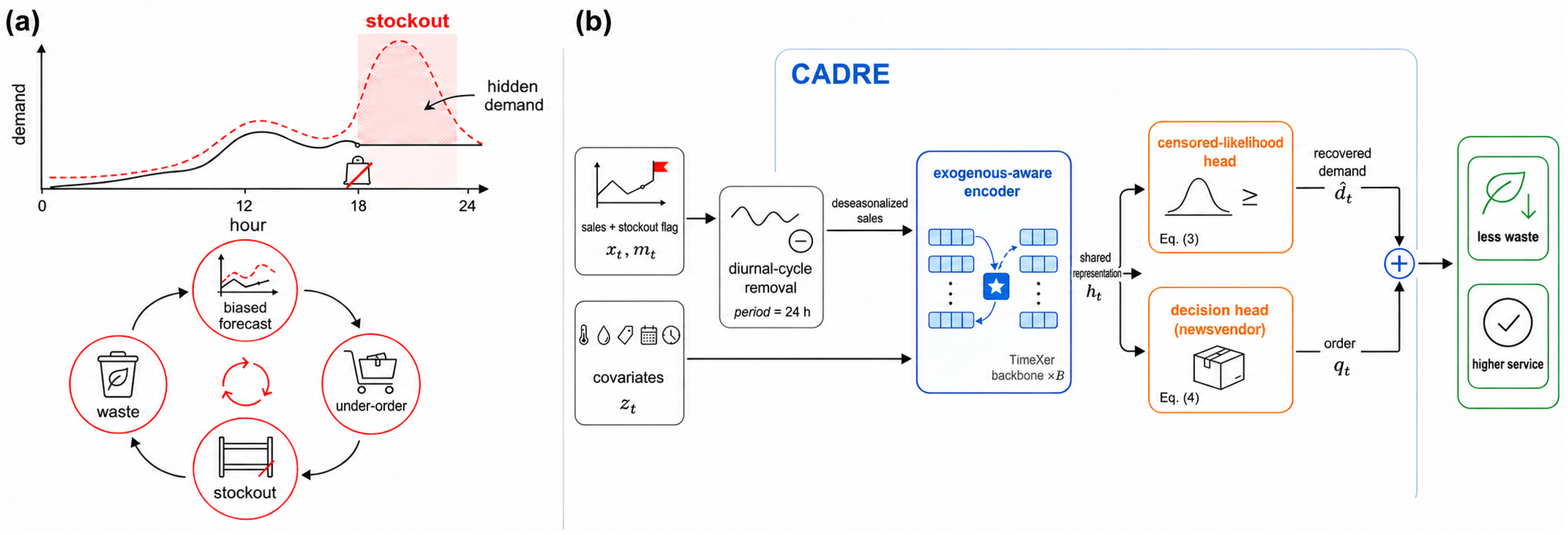
The apparent trade-off, however, rests on a flaw in the information the decision uses. A point-of-sale (POS) system records sales, not demand, and the two diverge precisely when a product sells out: the shelf empties, unmet demand goes unrecorded, and the sales log registers a low value even though demand did not fall. A forecaster trained on such records learns a biased relationship: it expects low demand where demand was merely unobserved, recommends a smaller order, and thereby induces the next stockout, which is again recorded as low demand. This is not random error that averages out, but a self-reinforcing bias in which under-ordering generates the observations that appear to justify further under-ordering. The distortion is worst where it is most costly: in FreshRetailNet-50K, a recent hourly benchmark, the share of store-hours in stockout rises from about 2 percent in the morning to roughly 26 percent at the evening peak, concentrating the corruption exactly where demand is largest [5,6].

Generic forecasters trained directly on censored sales may reproduce and reinforce this bias. The deep models now standard in retail are trained to reproduce the recorded series as closely as possible, so the better they fit, the more faithfully they reproduce its built-in bias [7,8,9]. Accuracy measured against censored sales is therefore not a sufficient training objective. Operations research understood the problem of demand hidden by stockouts long ago and built estimators to undo it [10,11,12,13], but those tools were designed for sparse, low-frequency records, and they stop at a corrected number, severed from the weather, promotions, and ordering decision that actually shape perishable demand. The unresolved methodological need is an approach that repairs the data and the decision together.

Three related streams each address part of this problem but leave the joint setting under-specified. Censored-demand and censored-newsvendor models correct for lost sales but are usually low-dimensional and ignore the high-frequency exogenous drivers shared across many store–stock-keeping-unit (SKU) series. Deep retail forecasters exploit covariates and shared structure but, trained on the recorded sales value, do not distinguish an uncensored low-demand hour from a stockout-censored one. Decision-focused inventory models train through replenishment costs but require an observed or externally estimated demand target. The unresolved question is whether censoring, exogenous forecasting and replenishment-oriented training can be handled within one probabilistic objective without scoring the model against its own imputed demand. CADRE tests this by combining a right-censored count likelihood, a cycle component estimated from non-stockout observations, and a newsvendor quantile loss trained on known demand (observed or re-censored with retained truth); the empirical tests then ask whether the lower-bound likelihood reduces recovery bias, whether the decision loss changes simulated replenishment beyond forecast accuracy, and whether in-model recovery improves on a two-stage impute-then-forecast pipeline.

This formulation begins by treating a stockout as an observation gap rather than as a measurement of low demand. Three consequences follow. If sold-out hours are missing rather than zero, a model should infer the demand that would have occurred instead of fitting the clamp. If demand carries a strong daily rhythm, that rhythm must be told apart from the gap, or an ordinary evening lull will be mistaken for scarcity. And if the purpose of a forecast is an order, the forecast should be judged by what that order wastes and what it fails to sell, not by an abstract error. CADRE, the model developed here, is an integrated implementation of these three design requirements in one deep network that reads sales together with their weather, promotion, and calendar context [14,15,16,17].

This reading reframes stockout censoring as a measurement problem for sustainable retail operations: when demand is systematically under-recorded at the peak, the resulting under-ordering may make the observed waste–availability trade-off appear less favourable than it would be under a less biased demand signal. The controlled experiments test whether correcting the censored demand signal can improve the modelled waste–availability frontier. On FreshRetailNet-50K, the re-censoring and replenishment simulation suggests that CADRE can reduce modelled waste while increasing simulated service level under the stated one-day shelf-life and lost-sales assumptions. The result does not establish that the same magnitude would occur in live operations; it identifies a mechanism, grounded in the quality of data retailers already hold, that should be tested in field deployment before it is claimed as an operational contribution to the United Nations Sustainable Development Goal (SDG) 12.3 target of halving food waste. Accordingly, this study makes three contributions. Methodologically, CADRE integrates a lower-bound censored likelihood, a stockout-protected diurnal-cycle representation, and known-truth decision regularisation within a shared exogenous forecaster; the individual elements are established, whereas their joint treatment of censoring, forecasting, and replenishment constitutes the original design. Empirically, the study uses a controlled re-censoring protocol and a matched two-stage comparison to evaluate recovery and replenishment against retained truth, while its sustainability contribution is limited to demonstrating potential decision-support benefits under the stated simulation assumptions. The remainder of the paper places the approach in prior work, develops the method, and reports the experiments that test each step of this argument.

2. Related Work

2.1. Deep Learning for Demand and Time-Series Forecasting

The retail forecasting literature moved from autoregressive and exponential-smoothing models to neural networks once large hierarchical sales panels became available, a transition documented by the M5 competition, where the leading entries combined gradient-boosted trees with neural components and where probabilistic accuracy, not point accuracy alone, decided the rankings [18,19]. Probabilistic recurrent models such as DeepAR established the template of predicting a full predictive distribution per series, which matters for inventory because the order quantity depends on a tail quantile rather than the mean [7], and the Temporal Fusion Transformer added interpretable attention over static and time-varying covariates [20]. Probabilistic demand forecasting of this kind has been deployed on production retail systems spanning millions of items [21]. The long-horizon Transformer line, beginning with Informer and Autoformer and continuing through FEDformer, attacked the quadratic cost of attention and the modelling of seasonality through sparsity and frequency-domain decomposition [22,23,24]. A subsequent reappraisal questioned whether attention was necessary at all: the linear DLinear model matched or beat heavier Transformers on several benchmarks [25], while PatchTST showed that patching and channel independence recovered the Transformer’s advantage [8], and TimesNet recast the series into a 2D representation to capture multiple periods [26]. iTransformer inverted the attention axis to treat variables as tokens, improving multivariate forecasts [9], and basis-expansion architectures such as N-BEATS and N-HiTS demonstrated that purely feed-forward stacks could be both accurate and interpretable [27,28]. These generic time-series forecasting models, when applied directly to point-of-sale records, normally optimise agreement with the recorded sales series and do not by themselves encode the stockout-specific lower-bound observation model considered in the censored-demand literature.

2.2. Forecasting with Exogenous Variables and Foundation Models

Perishable demand responds to drivers outside its own history, so the treatment of exogenous variables is central rather than incidental. TimeXer reconciles endogenous patches with exogenous variate tokens through a global bridging token and reports consistent gains on forecasting tasks that supply external regressors, which is the reason we adopt it as the backbone [15]. TimeMixer decomposes and mixes information across scales [29], and CycleNet models fixed periodicity with an explicit residual cycle that can be added to any predictor, a mechanism we borrow and adapt so that the censoring head is not burdened with periodic structure [16]. A parallel development trains a single model on large corpora for zero-shot transfer: TimesFM, Chronos, and Moirai forecast unseen series without per-dataset training [30,31,32]. These foundation models are attractive when local history is short, a common condition in emerging-market retail, and we include one as a zero-shot baseline. Their generic pretraining, however, has no notion of censoring and no access to the store-specific weather and promotion signals that move perishable sales, so they serve as a reference point rather than as a solution to the problem at hand.

2.3. Censored Demand, Lost Sales, and Demand Uncensoring

Estimating demand from sales that are truncated by availability is a classical concern. Tobin’s limited-dependent-variable model gave the canonical likelihood for a variable observed only above or below a threshold [14], and Conrad framed retail sales as a censored realisation of Poisson demand [10]. Nahmias analysed demand estimation under lost sales, where unmet demand vanishes without trace [11], and Sachs and Minner studied the data-driven newsvendor when only censored observations are available, showing that ignoring censorship biases the order quantity [12]. Nonparametric adaptive policies based on the Kaplan-Meier estimator learn ordering rules directly from censored sales [33], and the cost of the information that censoring destroys has been characterised through worst-case regret bounds [34]. Recent work has revisited the censored newsvendor with modern sample-complexity tools [35]. This stream provides the statistical foundation we build on, yet its models are typically low-dimensional, assume a single fixed demand distribution per item, and do not ingest high-frequency covariates or share structure across thousands of related series. Our contribution is to carry the censored-likelihood principle into a deep multivariate forecaster that does both.

2.4. Perishable Inventory and Decision-Focused Learning

The purpose of a demand forecast in this setting is an ordering decision under perishability, where over-ordering causes spoilage and under-ordering causes lost sales and lost goodwill [6,36]. When only the mean and variance of demand are known, the distribution-free newsvendor still yields a robust order rule [37], and the data-driven newsvendor connects estimation to this decision by fitting the order quantity directly to features [13,38]. Decision-focused learning generalises the idea: rather than minimising prediction error and optimising separately, it trains the predictor through the optimisation problem so that the loss reflects decision regret. Smart predict-then-optimize provides a convex surrogate for this regret [17], OptNet and task-based end-to-end learning differentiate through the optimisation layer [39,40], and a deployed end-to-end inventory model has shown the approach scales to real assortments [41]; a recent survey consolidates the gradient-based and gradient-free variants of this idea [42]. We adopt a differentiable newsvendor objective in this tradition, but train its auxiliary decision head only on observations whose demand is known—originally uncensored or artificially re-censored with retained truth—while genuine stockout observations contribute through the censored likelihood.

Table 1. Scope comparison of related methods. Entries summarise whether each stream, as typically formulated, treats stockouts as a lower bound on demand, ingests high-frequency exogenous covariates, shares a deep representation across many series, trains for the ordering decision, is evaluated without scoring against its own imputed demand, and reports a waste or sustainability simulation.

Method Stream	Censoring as Lower Bound	High-Freq. Exog. Covariates	Shared Deep Representation	DeciSion-Oriented Training	Not Scored on Own Imputation	Waste Sustainability Simulation
Tobit/Poisson censored estimators	Yes	Limited	No	No	Partly	No
Lost-sales demand estimation	Yes	Limited	No	Sometimes	Partly	No
Censored newsvendor/Kaplan–Meier	Yes	Limited	No	Yes	Theory/simulation	No
Generic deep retail forecasters	No	Yes	Yes	No	Yes (observed sales)	No
Decision-focused inventory learning	Usually no	Sometimes	Yes	Yes	Depends on labels	Sometimes
Two-stage recovery pipeline	Yes	Yes	Partly	Sequential	Yes (re-censoring)	Limited
CADRE (this work)	Yes	Yes	Yes	Yes	Yes (re-censoring)	Model-based

places these streams side by side along the properties that matter for stockout-censored fresh retail. Each stream resolves part of the setting: the censored-demand literature encodes the lower-bound observation model, deep retail forecasters exploit shared representations and high-frequency covariates, and decision-focused inventory models train through the ordering cost. The comparison therefore positions CADRE as an integrative design rather than as a claim that its individual backbone, likelihood, cycle module, or decision loss is new. The originality claimed here lies in the shared training architecture, the known-truth decision target, and the controlled evaluation protocol that avoids scoring the model against its own imputation.

3. The CADRE Framework

3.1. Problem Formulation and Overview

Consider a single store-product series observed at hourly resolution. At hour t the point-of-sale system records sales $x_t\in {\mathbb{Z}}_{\ge 0}$ and a stockout flag $m_t\in \{0,1\}$, where $m_t=1$ marks an hour in which the item was unavailable for part or all of the interval. The quantity of interest is the latent demand $d_t$, the units customers would have bought had stock been unlimited. The two observables relate to it through a censoring rule: when $m_t=0$ the record is exact, $x_t=d_t$; when $m_t=1$ the record is a lower bound, $d_t\ge x_t$. Sales therefore furnish a right-censored view of demand, and the censoring rate rises through the day with depletion. Alongside each hour the dataset supplies an exogenous vector ${\mathit{z}}_t\in {\mathbb{R}}^c$ holding temperature, precipitation, promotional discount, a holiday indicator, and cyclical encodings of hour-of-day and day-of-week.

The stockout flag is an interval-level availability indicator: we set $m_t=1$ whenever the benchmark marks the item unavailable at any point in the hour, and $m_t=0$ otherwise. The public fields give no within-hour duration or inventory-on-hand, so partial- and full-hour stockouts share one weight and a flagged hour contributes the conservative lower-bound event $D_t\ge x_t$ rather than a point value. Given an availability fraction $a_t$, Equation (3) could be replaced by an exposure-aware (binomial-thinning or interval-censoring) likelihood.

Only covariates available at forecast-creation time are used over the horizon. Calendar variables and planned promotions are known in advance; weather uses a causal day-ahead persistence proxy from the latest observed day. An upper-bound “oracle weather” variant that substitutes realised future weather is reported only as a sensitivity check (Appendix F), so no future information leaks into the main comparison.

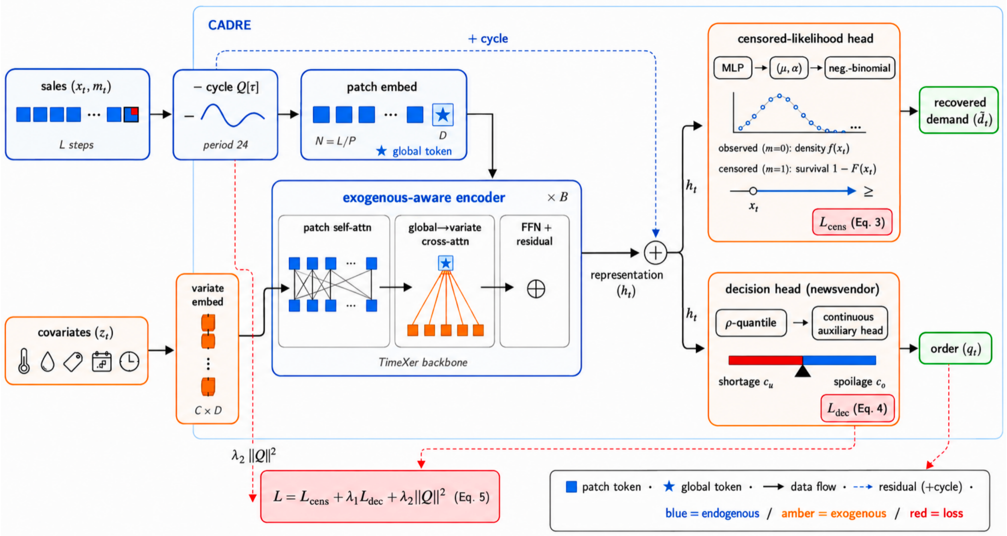
The task has two coupled parts. The first is recovery: infer the latent demand ${\widehat{d}}_t$ on censored hours from the uncensored hours, the covariates, and the shared structure across series. The second is decision: forecast demand over a future horizon of H hours from a lookback window of L hours, and turn that forecast into a replenishment quantity that minimises the combined cost of spoilage and shortage. CADRE addresses both with one shared encoder, a diurnal-cycle module, and two heads. Figure 1 sketches the pipeline: covariate-conditioned sales enter an exogenous-aware encoder, a diurnal-cycle module removes and later restores the fixed daily rhythm, a censored-likelihood head recovers latent demand, and a decision head maps the predictive distribution to an order quantity scored by a newsvendor cost. Present tense describes the model throughout this section; experimental outcomes are reported in the past tense later. The framework is evaluated through three separate questions: whether the censored likelihood reduces latent-demand bias, whether the decision loss changes replenishment outcomes beyond forecast accuracy, and whether the end-to-end formulation outperforms a two-stage recovery-then-forecast pipeline under identical re-censoring masks.

Table 2. Key notation used in the CADRE framework. Symbols not listed are defined where they are introduced.

Symbol	Meaning
$x_t$	observed sales at time t
$m_t$	stockout/censoring flag (1 if censored)
$d_t$	latent demand under full availability
${\mathit{z}}_t$	known exogenous covariates
$L,H$	lookback and forecast horizon
$\mathit{Q}$	diurnal-cycle bank
${\mu }_t,{\alpha }_t$	negative-binomial mean and dispersion
$S_t\left(x\right)$	survival probability $Pr(D_t\ge x)$
${\tilde{d}}_t$	decision target (observed or re-censored known demand)
$q_t$	auxiliary decision-head output (training-only regulariser)
$\rho$	critical fractile $c_u/(c_u+c_o)$
${\lambda }_1,{\lambda }_2$	decision-loss and cycle-regularisation weights

summarises the symbols used most frequently below.

3.2. Exogenous-Aware Encoder

The encoder follows TimeXer’s separation of endogenous and exogenous information [15]. The deseasonalised target series, defined in the next subsection, is split into $N=\lceil L/P\rceil$ non-overlapping patches of length P. Each patch is linearly embedded into a D-dimensional token, and a single learnable global token $\mathit{g}$ is appended to summarise the series. Patch tokens attend to one another and to $\mathit{g}$ through standard self-attention [43], capturing intra-series temporal dependence. Each exogenous channel in ${\mathit{z}}_t$ is embedded as one variate token; the global token $\mathit{g}$ attends across the variate tokens through cross-attention, so external drivers reach the endogenous representation only by way of $\mathit{g}$. This asymmetry keeps the parameter count near linear in the number of covariates while still letting a rainfall spike or a promotion shift the forecast. Writing $\mathit{H}$ for the stack of patch tokens and the global token, one pre-norm encoder block computes

$$\begin{array}{cc}\hfill {\mathit{H}}^{\mathrm{sa}}& =\mathit{H}+\mathrm{SelfAttn}\left(\mathrm{LN}\right(\mathit{H}\left)\right),\hfill \\ \hfill {\mathit{g}}^{\mathrm{sa}}& =\mathrm{Global}\left({\mathit{H}}^{\mathrm{sa}}\right),\hfill \\ \hfill {\mathit{g}}^{\mathrm{ca}}& ={\mathit{g}}^{\mathrm{sa}}+\mathrm{CrossAttn}\left(\mathrm{LN}\left({\mathit{g}}^{\mathrm{sa}}\right),{\mathit{E}}_z,{\mathit{E}}_z\right),\hfill \\ \hfill \tilde{\mathit{H}}& =\mathrm{ReplaceGlobal}({\mathit{H}}^{\mathrm{sa}},{\mathit{g}}^{\mathrm{ca}}),\hfill \\ \hfill {\mathit{H}}^{+}& =\tilde{\mathit{H}}+\mathrm{FFN}\left(\mathrm{LN}\left(\tilde{\mathit{H}}\right)\right),\hfill \end{array}$$

(1)

where $\mathrm{LN}$ denotes layer normalisation, ${\mathit{E}}_z$ are the exogenous variate tokens and $\mathrm{FFN}$ is a position-wise feed-forward network. Here $\mathrm{Global}(·)$ extracts the learnable global token after self-attention and $\mathrm{ReplaceGlobal}(·)$ inserts the cross-attended global token back into the token stack, so external drivers reach the endogenous representation only through $\mathit{g}$; this notation avoids a self-referential update and fixes the residual order used in the implementation. Stacking B such blocks and applying the horizon decoder described below yields a contextual representation ${\mathit{h}}_t$ per future hour, which the two heads consume.

Table 3. Encoder tensor shapes and structural settings for one minibatch of $\left|\mathcal{B}\right|$ series.

Component	Shape/Setting
Target input	$\left|\mathcal{B}\right|\times L\times 1$
Future covariates	$\left|\mathcal{B}\right|\times H\times c$
Patch tokens	$\left|\mathcal{B}\right|\times N\times D$, with $N=\lceil L/P\rceil$
Global token	$\left|\mathcal{B}\right|\times 1\times D$
Exogenous tokens	$\left|\mathcal{B}\right|\times c\times D$
Horizon decoder	linear $(N+1)D\to HD$, reshaped to $\left|\mathcal{B}\right|\times H\times D$
Position encoding	learnable patch position + hour-of-day phase embedding
Residual order	pre-LN attention and feed-forward residuals
Output heads	NB likelihood head: linear maps to ${\mu }_t,{\alpha }_t$ (deployment order from the NB predictive distribution, Section 4.4); auxiliary decision head: continuous $q_t=\mathrm{softplus}\left({\mathit{w}}_q^{\top }{\mathit{h}}_t\right)$, a training-only regulariser

fixes the tensor shapes needed for reproduction: after per-series normalisation the deseasonalised target is split into $N=\lceil L/P\rceil$ patches with a learnable global token and patch positional embeddings, each exogenous channel is embedded as one variate token, and after B pre-norm blocks the token stack is projected to H horizon tokens by a linear decoder to which future-covariate and hour-of-day phase embeddings are added before the two heads.

3.3. Diurnal-Cycle Decomposition

Hourly perishable sales carry a near-deterministic 24-h rhythm: a morning rise, a midday plateau, and an evening peak. Because stockouts cluster in that evening peak, a censoring head fitted to raw sales risks attributing the periodic dip after the peak to missing demand. To prevent that confusion we remove the cycle before encoding and add it back afterwards, adapting the residual-cycle mechanism of CycleNet [16]. A learnable bank $\mathit{Q}\in {\mathbb{R}}^{c_{\mathrm{p}}\times 1}$ stores one offset per phase of the period $c_{\mathrm{p}}=24$. For an hour with phase index $\tau \left(t\right)=tmod{c}_{\mathrm{p}}$ the deseasonalised input is

$${\tilde{x}}_t=x_t-\mathit{Q}\left[\tau \left(t\right)\right],$$

(2)

and the head outputs are recentred by the matching offset before the likelihood and decision terms are evaluated. Because evening stockouts are exactly where the daily profile is largest, a cycle bank fitted freely to raw sales could absorb the stockout-induced depression as if it were normal seasonality. To prevent this, each phase offset is initialised from uncensored hours only,

$${\mathit{Q}}^{\left(0\right)}\left[k\right]=median\left\{x_{i,t}-{\overline{x}}_i:\tau \left(t\right)=k,m_{i,t}=0\right\},$$

For any stockout-flagged hour, gradients from all loss terms that use that hour, including both the censored likelihood and the decision loss, are stopped from reaching the corresponding cycle entry $\mathit{Q}\left[\tau \right(t\left)\right]$. The cycle bank is therefore updated only by uncensored-hour terms and by the regulariser in Equation (5). The bank is shared across series within a category, so it absorbs the stable part of the daily shape and leaves the encoder to model covariate-driven and stochastic variation. This separation is what allows the censoring head to interpret a late-evening shortfall as censorship rather than as the normal post-peak decline. The protected bank reaches 36.71 WAPE ($-1.3$ bias, 6.4 waste), against 37.21 ($-1.9$, 6.8) for an unmasked end-to-end bank and 37.84 ($-2.4$, 7.1) with no cycle module. Figure 2 shows the complete CADRE architecture, in which the diurnal-cycle module connects to the shared encoder and the two output heads.

3.4. Censored Demand Recovery Head

The recovery head predicts a demand distribution per hour and trains it with a likelihood that respects censoring. We model latent demand as negative-binomial (NB), a natural choice for over-dispersed non-negative counts, with the encoder producing the mean ${\mu }_t=\mathrm{softplus}\left({\mathit{w}}_{\mu }^{\top }{\mathit{h}}_t\right)$ and dispersion ${\alpha }_t=\mathrm{softplus}\left({\mathit{w}}_{\alpha }^{\top }{\mathit{h}}_t\right)$. Let $f(·;{\mu }_t,{\alpha }_t)$ be the negative-binomial probability mass function and $F(·;{\mu }_t,{\alpha }_t)$ its cumulative distribution. The distribution is parameterised by the mean ${\mu }_t>0$ and over-dispersion ${\alpha }_t>0$, giving $\mathrm{Var}\left(D_t\right)={\mu }_t+{\alpha }_t{\mu }_t^2$; equivalently, with size $r_t=1/{\alpha }_t$ and probability $p_t=r_t/(r_t+{\mu }_t)$, the support is $y\in \{0,1,2,\dots \}$ and

$$Pr(D_t=y)={\displaystyle \frac{\Gamma (y+r_t)}{\Gamma \left(r_t\right)y!}}{p}_t^{r_t}{(1-p_t)}^y.$$

The censored term uses the survival probability $S_t\left(x_t\right)=Pr(D_t\ge x_t)=1-F(x_t-1;{\mu }_t,{\alpha }_t)$. The per-hour loss splits on the stockout flag,

$${\ell }_t^{\mathrm{cens}}=-(1-m_t)logf(x_t;{\mu }_t,{\alpha }_t)-m_{t}log\left(1-F(x_t-1;{\mu }_t,{\alpha }_t)\right),$$

(3)

so an uncensored hour contributes the ordinary log-likelihood of the recorded value, while a censored hour contributes only the survival probability $Pr(D\ge x_t)$, the statement that true demand was at least what was sold. Equation (3) is the Tobit likelihood [14] written for a count distribution and evaluated per series by the shared encoder. The recovered demand on a censored hour is the posterior mean ${\widehat{d}}_t=\mathbb{E}[D\mid D\ge x_t]$, computed from the fitted distribution and reported as the recovered demand for the recovery metrics of Section 5.9; it is not used as a training target for the order head (Section 3.5). For numerical stability the log-survival $log{S}_t\left(x_t\right)$ is evaluated in log-space with a lower clamp of ${10}^{-12}$, and the posterior mean is obtained from the negative-binomial tail identity

$$\mathbb{E}[D_t\mid D_t\ge x_t]={\mu }_t{\displaystyle \frac{S_{r_t+1,p_t}(x_t-1)}{S_{r_t,p_t}\left(x_t\right)}},$$

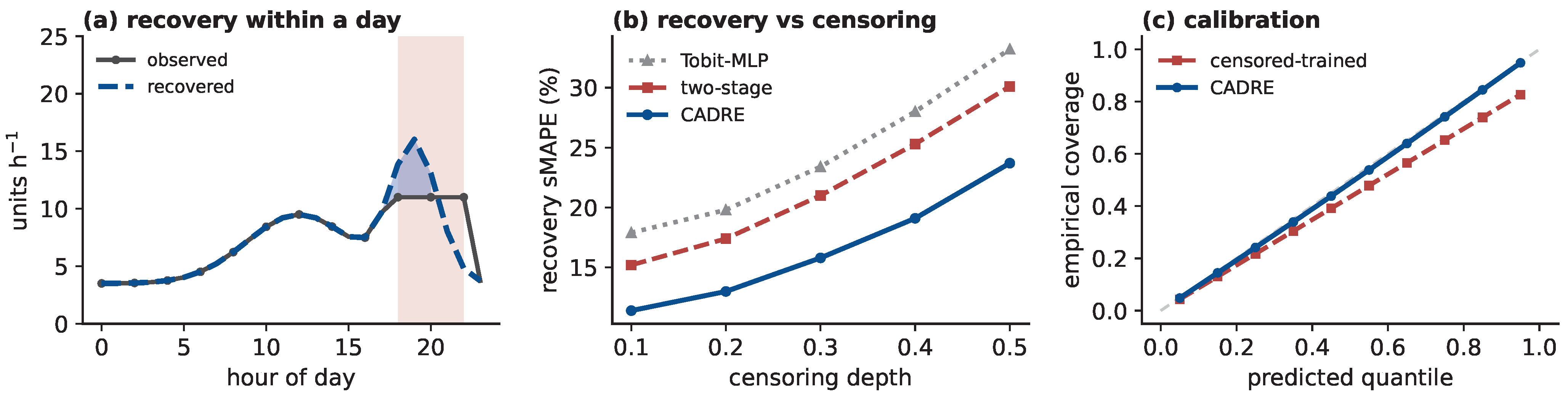
where $S_{r,p}(·)$ is the survival function of a negative binomial with size r and probability p; a truncated sum up to the $1-{10}^{-8}$ quantile serves as an independent check, and the two agree to a relative error below ${10}^{-6}$ (Appendix D). Treating stockout hours through Equation (3) rather than as observed counts is the single change that removes the structural downward bias; Figure 3 contrasts the recovered curve with the censored record across stockout depth.

3.5. Decision-Focused Replenishment Loss

A forecast that is accurate in squared error can still order badly, because the cost of an ordering mistake is asymmetric: a unit of unsold perishable is wasted, while a unit of unmet demand is a lost sale. The newsvendor model captures this asymmetry through an understock cost $c_u$ and an overstock cost $c_o$, with optimal order at the critical fractile $\rho =c_u/(c_u+c_o)$ [6,13]. CADRE regularises the shared representation with a continuous, differentiable auxiliary decision head, $q_t=\mathrm{softplus}\left({\mathit{w}}_q^{\top }{\mathit{h}}_t\right)$, that is used only during training and never at deployment; the deployment order is formed entirely from the negative-binomial predictive distribution as described in Section 4.4, so the auxiliary head requires no discrete inverse CDF and no gradient passes through a discrete step function. The auxiliary head is trained by the pinball loss only where the true demand is known: on uncensored hours, where the target is ${\tilde{d}}_t=x_t=d_t$, and on training hours whose target-horizon values are artificially re-censored by the operator of algorithm in Section 4.1 with their true value $y_t$ retained as the target. Genuine stockout hours, whose latent demand is unknown, are excluded from the decision loss and enter only the censored likelihood. Writing $\mathcal{K}$ for this known-truth set,

$${\ell }_t^{\mathrm{dec}}=\mathbf{1}[t\in \mathcal{K}]\left(c_u{({\tilde{d}}_t-q_t)}_{+}+c_o{(q_t-{\tilde{d}}_t)}_{+}\right),{\tilde{d}}_t=d_t(\mathrm{known}\mathrm{truth}),$$

(4)

where ${(·)}_{+}$ denotes the positive part. Equation (4) is the pinball loss at level $\rho$, convex and differentiable almost everywhere in $q_t$, and minimising it shapes the shared representation toward cost-aware ordering [17,40]. The auxiliary head and its loss update only the shared encoder and the head parameters; the decision term reaches the negative-binomial likelihood head only indirectly, through the representation ${\mathit{h}}_t$, and the deployment order is read from that likelihood head rather than from $q_t$. Because the decision target on every hour that enters the pinball loss is a known true value rather than a model-generated quantity, the auxiliary head is never trained against the model’s own imputed demand; the recovered posterior mean of Section 3.4 is used to report recovery, not as a decision target, which removes both the self-referential-training risk and the tendency of a posterior-mean target to pull the high quantile toward the conditional mean. The censored likelihood of Equation (3) remains the sole source of learning on genuine stockout hours. This separates training circularity from evaluation circularity: training uses only known-truth targets, and recovery and replenishment are evaluated only on re-censored hours whose truth is known, so nothing reported is scored against CADRE’s own imputation. Pseudo-target alternatives—censored sales as the target, a stop-gradient recovered target, or a non-detached recovered target—are compared in the ablation study (Section 5.2).

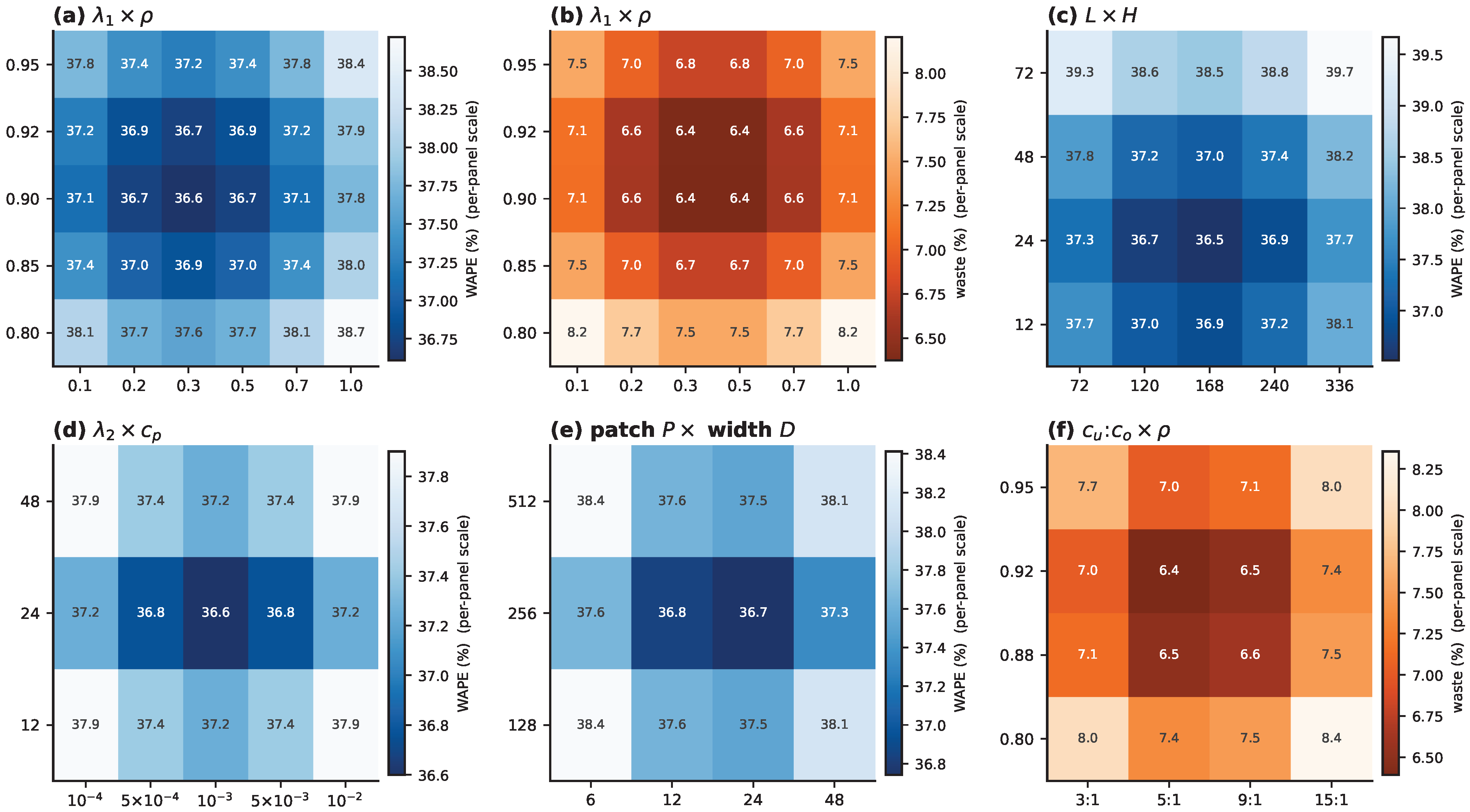
The ratio $c_u/c_o$ is a managerial cost scenario rather than a property of perishability alone. A shorter shelf life can raise $c_o$ and lower the optimal fractile, whereas high lost-sales, substitution or goodwill costs can raise $c_u$ and lift it. The main text reports $\rho =0.90$ as a high-service scenario for staple perishables and reports additional fractiles in Section 5.4. We distinguish the training fractile ${\rho }_{\mathrm{train}}$—the pinball level at which the order head is fitted, a hyperparameter that requires retraining to change—from the deployment fractile ${\rho }_{\mathrm{deploy}}$—the quantile read from a fixed trained model at order time. Both default to $0.90$; Figure 4a,b varies ${\rho }_{\mathrm{train}}$ with per-cell retraining, whereas the deployment-fractile sweep in Section 5.5 varies only ${\rho }_{\mathrm{deploy}}$. For a clean and comparable comparison across methods, the main experiments fix a single representative critical fractile rather than tuning it per category; the sensitivity study in Section 5.4 then sweeps the shortage-to-spoilage ratio to trace how a shelf-life-dependent cost would shift the waste outcome.

3.6. Joint Training Objective and Optimisation

The two heads share the encoder and the cycle bank and are trained jointly. Summing over the hours of a series and averaging over a minibatch gives

$$\mathcal{L}={\displaystyle \frac{1}{\left|\mathcal{B}\right|}}\sum _{i\in \mathcal{B}}\sum _t\left({\ell }_t^{\mathrm{cens}}+{\lambda }_1{\ell }_t^{\mathrm{dec}}\right)+{\lambda }_2{\parallel \mathit{Q}\parallel }_2^2,$$

(5)

where ${\lambda }_1$ balances forecast likelihood against decision cost and ${\lambda }_2$ regularises the cycle bank to discourage it from absorbing non-periodic variation. We optimise Equation (5) with AdamW under a cosine schedule. Because the censored term and the decision term are optimised jointly over one shared representation, no separate imputation stage is needed, and the decision loss is applied only on hours with known truth (uncensored and training-re-censored), so it never uses a model-generated target, while the censored likelihood of Equation (3) remains the source of distributional learning for genuine stockout observations. This end-to-end coupling is the practical difference from a two-stage pipeline that first imputes demand and then forecasts it, and the ablation in Section 5.2 isolates the contribution of each term in Equation (5).

3.7. Complexity

With lookback L, patch length P, and width D, one encoder block costs $\mathcal{O}\left({(L/P)}^{2}D+(L/P)D^2\right)$ for self-attention and $\mathcal{O}\left(c{D}^2\right)$ for cross-attention over c covariates, identical in order to the TimeXer backbone. The cycle bank adds $c_{\mathrm{p}}$ parameters and a constant-time lookup per hour. The two heads are linear maps from ${\mathit{h}}_t$, and the survival term in Equation (3) evaluates a regularised incomplete beta function whose cost is independent of sequence length. CADRE therefore retains the backbone’s complexity while adding parameters that scale with the period length rather than with the data size, which is what keeps training time within a few minutes per epoch at the scale reported in Section 5.8.

4. Datasets and Experimental Setup

4.1. Datasets

The primary benchmark is FreshRetailNet-50K, released in 2025 as the first public fresh-retail dataset with explicit stockout annotation [5]. It contains 50,000 store-product time series sampled hourly over roughly ninety-day windows, drawn from 863 perishable SKUs across 898 stores in 18 Chinese cities, for close to 100 million observations in total. Each hour carries the recorded sales, a stockout flag, a promotional-discount level, and store-local weather, with daily temperature and precipitation collected per location and Chinese statutory holidays labelled; store identifiers are pseudonymised in the public release. The data exhibits the structure that motivates our design. Sales are concentrated, with 20 percent of SKUs accounting for 51.8 percent of transactions, demand carries a pronounced daily cycle and a 27 percent holiday surge, and stockout incidence climbs from about 2 percent of store-hours in the early morning to roughly 26 percent by eight in the evening, so censoring is heaviest precisely at the demand peak. These figures are reported by the dataset authors and we reproduce the relevant ones in

Table 4. Dataset roles and evidential scope. FreshRetailNet-50K provides real hourly stockout flags and supports censored-demand modelling and controlled replenishment evaluation [5]; the Favorita panel contains no observed stockout labels and is used only for daily robustness under a constructed high-demand mask, accessed through the LOTSA mirror.

Property	FreshRetailNet-50K	Corp. Favorita (Ecuador)
Region	18 cities, China	54 stores, Ecuador
Granularity	Hourly	Daily
Series	50,000	Store–family, daily
SKUs/families	863 SKUs	33 families
Samples	≈100 million hourly observations	≈120 M item–day rows (≈3 M family–day fitted)
Span per series	≈90 days	2013–2017
Stockout labels	Real, hourly	None
Covariates	temp., precip., discount, holiday	promotion, oil price, holiday
Censoring in experiments	real labels for training; controlled re-censoring for known-truth evaluation	constructed high-demand, day-level mask
Evidence role	primary stockout-censored fresh-retail benchmark	cross-market daily robustness check
Supports	stockout recovery; intraday peak censoring; replenishment simulation	robustness to market and cadence under synthetic censoring
Does not support	direct field waste measurement	real stockout recovery or intraday claims

.

To test whether the method survives a change of market and assortment, we add Corporación Favorita grocery sales from Ecuador, a daily record of item-level sales across 54 stores and 33 product families between 2013 and 2017, with promotion, oil-price, and national-holiday covariates. We access it through the Apache-licensed LOTSA mirror rather than any restricted source [32]. Favorita is daily and records no stockouts, so it cannot resolve intraday demand and offers no ground truth for recovery; instead we impose a constructed censoring mask that hides a fraction of each series’ highest-demand days, which lets us measure forecasting robustness under known daily censoring while being explicit that the mask is constructed rather than observed. The default mask hides the top $\pi =20\%$ of high-demand days per series, a rate chosen to be of the same order as the evening stockout incidence observed in FreshRetailNet and large enough to induce a measurable downward bias; its choice is not tuned to any result, and Appendix G reports the sensitivity to the mask rate and to random and demand-proportional mask types. Because the censoring here is synthetic and the granularity is daily, we treat Favorita as supporting cross-market evidence rather than as a second stockout benchmark, and we make no intraday or evening-peak claim for it.

The negative-binomial head models a non-negative count-scale target, so the preprocessing is stated explicitly and the count assumption is not treated as load-bearing. FreshRetailNet does not publish raw integer units: the public fields (sale_amount, hours_sale) are non-negative globally normalised floating-point sales. We therefore invert the release’s per-series scaling where a coefficient is available and otherwise rescale each series to a common count-like scale, remove negative returns, insert missing store–SKU–hour cells as zeros when the SKU is active, and round to the nearest unit for the negative-binomial head; the residual non-integer values that remain before rounding are a small minority and, as shown below, do not drive the result. Favorita is aggregated to store–family–day totals (about 3 million series–day cells, from roughly 120 million raw item–day records), with negative returns removed and totals rounded to the nearest unit. To confirm that the count-likelihood choice is not load-bearing on either dataset, Appendix H refits the recovery head with a Tweedie and a log-normal likelihood on the unrounded normalised values of FreshRetailNet and Favorita alike; the method ranking is unchanged, so the negative-binomial support assumption is a modelling convenience rather than a claim about the raw units.

We split each series chronologically into the first 70 percent of its span for training, the next 10 percent for validation, and the final 20 percent for testing, which for a ninety-day FreshRetailNet series is roughly 63, 9, and 18 days, so that no future information informs model selection. Because true demand on genuinely sold-out hours is never observed, we separate the results into three regimes and state the target variable in each. The first is forecasting on observable demand: accuracy is measured only on test hours that are not stocked out, where the record equals true demand ($m_t=0$, so $x_t=d_t$), and every method is scored against the same observed values. The second is controlled recovery: we take uncensored test hours whose value is known, artificially re-censor a fraction of them, and measure how well each method reconstructs the hidden truth. The third is a model-based replenishment simulation, run on the controlled re-censoring bed so that orders are settled against known true demand rather than against any method’s own reconstruction. This design keeps the evaluation free of circularity: CADRE is never scored against demand that CADRE itself imputed. Algorithm 1 specifies the controlled re-censoring procedure that constructs the second and third regimes.

Algorithm 1. Controlled re-censoring for known-truth recovery and replenishment evaluation

Input: per-series test observations ${\left\{(x_t,m_t)\right\}}_{t\in {\mathcal{T}}_i}$; mask rate $\pi$; seed s; stratum map $\sigma$ (hour-of-day for FreshRetailNet, day-of-week for Favorita). Output: shared re-censored inputs $\left\{(x_t^{\mathrm{cen}},m_t^{\mathrm{cen}})\right\}$ and known truth $\left\{y_t\right\}$.   1: for each store–SKU series i do   2:     ${\mathcal{C}}_i\leftarrow \{t\in {\mathcal{T}}_i:m_t=0,x_t>0\}$;   $y_t\leftarrow x_t$    ▹ candidates, known truth   3:     $x_t^{\mathrm{cen}}\leftarrow x_t,m_t^{\mathrm{cen}}\leftarrow m_t$ for all $t\in {\mathcal{T}}_i$    ▹ default: original flag preserved   4:     for each calendar stratum k do   5:         ${\mathcal{C}}_{ik}\leftarrow \mathrm{sort}\left(\{t\in {\mathcal{C}}_i:\sigma \left(t\right)=k\},\mathrm{by}{y}_t\mathrm{descending}\right)$   6:         ${\mathcal{S}}_{ik}\leftarrow$ first $\lceil \pi \left|{\mathcal{C}}_{ik}\right|\rceil$ elements of ${\mathcal{C}}_{ik}$    ▹ ties: seed-s permutation   7:         for each $t\in {\mathcal{S}}_{ik}$ do   8:            ${\delta }_t\sim \mathrm{Uniform}(0.20,0.60)$   9:            $x_t^{\mathrm{cen}}\leftarrow \lfloor (1-{\delta }_t)y_t\rfloor$;   $m_t^{\mathrm{cen}}\leftarrow 1$    ▹ partial-depth censoring  10:         end for  11:     end for  12: end for  13: present the identical $\left\{(x_t^{\mathrm{cen}},m_t^{\mathrm{cen}})\right\}$ to every model  14: score all recovery and replenishment metrics against $y_t$ only    ▹ never against a model output  15: return$\left\{(x_t^{\mathrm{cen}},m_t^{\mathrm{cen}})\right\},\left\{y_t\right\}$

The controlled bed uses mask rate $\pi =0.20$ by default; Section 5.3 sweeps the mask rate $\pi \in \{0.10,0.20,0.30,0.40,0.50\}$ (the fraction of candidate hours masked) at fixed per-hour depth $\delta$∼$\mathrm{U}(0.20,0.60)$ and also reports the effect of the mask type, while the sensitivity to censoring depth $\delta$ is the recovery-error curve of Figure 3b. Within each calendar stratum the mask holds $\pi$ fixed and hides the highest-demand hours, which concentrates censoring on high-demand values but does not reproduce the way real stockout incidence rises across the day (about 2% in the morning to 26% in the evening); to reproduce that rising incidence we additionally evaluate an incidence-weighted depletion mask whose per-stratum rate is set proportional to the observed hour-of-day stockout incidence (Section 5.3). Highest-demand masking remains the most favourable case for a censoring-aware method, which is why uniform-random, demand-proportional and incidence-weighted masks are reported alongside it. Because the latent demand on genuinely stockout-flagged hours is unknown, the known truth $y_t$ exists only for candidate (originally-uncensored) hours; recovery and replenishment metrics are therefore computed over these known-truth hours, including the re-censored subset, while genuine stockout hours retain their observed flag $m_t$ and are not counted as known truth. Two further differences from real stockouts remain. The mask reduces individual high-demand hours by a random fraction $\delta$, whereas a genuine stockout empties the shelf and censors several consecutive hours completely, so the bed models shallower and less clustered censoring than the evening depletions it stands in for; and because the hidden truth must be known, the bed can only draw from hours that were not actually stocked out, which excludes the most severely censored evening-peak hours by construction. The controlled bed therefore measures recovery against known truth under a conservative, favourable approximation of the real mechanism rather than reproducing the depletion dynamics themselves, so a field trial remains necessary to confirm recovery under real consecutive-hour stockouts.

4.2. Baselines

The comparison spans four families. The statistical reference is seasonal autoregressive integrated moving average (SARIMA) fitted per series. The deep point-forecast family includes DLinear [25], N-HiTS [28], PatchTST [8], TimesNet [26], and iTransformer [9]. The exogenous-aware and probabilistic family includes DeepAR [7] and the vanilla TimeXer backbone without our heads [15], which isolates the value of the censoring and decision components. A zero-shot foundation model, Chronos, is run without fine-tuning to gauge how far generic pretraining travels on this domain [31]. The censoring-aware family contains a Tobit regression with a shared multilayer perceptron (MLP) [14] and the two-stage impute-then-forecast pipeline reported with the dataset, which first reconstructs demand on stockout hours and then trains a standard forecaster on the reconstruction [5]. All learned baselines use the same chronological splits, lookback and horizon, target normalisation and early-stopping rule. Hyperparameters are selected from a small validation grid rather than from a single default. Models with native support for future covariates receive the same calendar, promotion and causal-weather covariates as CADRE; for models without native future-covariate support this limitation is recorded in

Table A1. Baseline implementation and tuning protocol for the methods in Table 7. Repository entries give the GitHub project and the exact version used—the short-SHA main-branch commit or the model checkpoint—accessed in July 2026. All learned models use seeds 0–4 and the shared splits, lookback, horizon and normalisation; point-model decision quantiles use per-series additive validation-residual calibration.

Model	Source/Commit	Covariates Supplied	Validation Grid (Candidate Values)	Early Stopping	Decision Quantile
SARIMA	statsmodels 0.14.6; pmdarima 2.1.1	none; seasonal period 24 (FRN)/7 (Fav)	$p,q\in \{0,1,2\}$; $d,P,D,Q\in \{0,1\}$	validation WAPE	empirical residual $\rho$-quantile
DLinear	cure-lab/LTSF-Linear 0c11366	target history (no future cov.)	lr $\{{10}^{-3},5\times {10}^{-4},{10}^{-4}\}$; batch $\{32,64,128\}$; dropout $\{0,0.1,0.2\}$	validation WAPE	per-series residual $\rho$-quantile
N-HiTS	Nixtla NeuralForecast 1.7.2 b9e4d02	calendar/promotion (native)	lr $\{{10}^{-3},5\times {10}^{-4}\}$; batch $\{32,64\}$; stacks $\{2,3\}$; width $\{256,512\}$	validation WAPE	per-series residual $\rho$-quantile
PatchTST	yuqinie98/PatchTST 204c21e	target-only (no future cov.)	lr $\{{10}^{-3},5\times {10}^{-4},{10}^{-4}\}$; batch $\{64,128\}$; patch $\{8,16,24\}$; dropout $\{0,0.1,0.2\}$	validation WAPE	per-series residual $\rho$-quantile
TimesNet	thuml/Time-Series-Library d8f2a17	calendar/promotion/weather channels	lr $\{{10}^{-3},5\times {10}^{-4}\}$; batch $\{32,64\}$; $d_{\mathrm{model}}\{32,64\}$; top-k $\{3,5\}$	validation WAPE	per-series residual $\rho$-quantile
iTransformer	thuml/Time-Series-Library d8f2a17	covariates as variate tokens	lr $\{{10}^{-3},5\times {10}^{-4}\}$; batch $\{32,64\}$; $d_{\mathrm{model}}\{256,512\}$; layers $\{2,3\}$	validation WAPE	per-series residual $\rho$-quantile
DeepAR	GluonTS 0.16.2 (PyTorch)	past/future known covariates	lr $\{{10}^{-3},5\times {10}^{-4}\}$; batch $\{32,64\}$; hidden $\{40,80\}$; layers $\{2,3\}$	validation NLL	predictive $\rho$-quantile (200 samples)
TimeXer	thuml/Time-Series-Library d8f2a17	calendar/promotion/causal weather	lr $\{{10}^{-3},5\times {10}^{-4},{10}^{-4}\}$; batch $\{32,64,128\}$; dropout $\{0,0.1,0.2\}$	validation WAPE	predictive/residual $\rho$-quantile
Chronos	amazon/chronos-t5-base (∼200 M)	target only, zero-shot	context 512 (FRN)/64 (Fav); 100 samples; temp $1.0$; per-series scaling	n/a (zero-shot)	sample $\rho$-quantile
Tobit-MLP	authors’ PyTorch impl.	same covariates as CADRE	lr $\{{10}^{-3},5\times {10}^{-4}\}$; batch $\{64,128\}$; hidden $\{128,256\}$; layers $\{2,3\}$	validation censored NLL	predictive $\rho$-quantile
Two-stage	stage 1: CADRE NB censored head; stage 2: TimeXer d8f2a17 (both retrained)	same covariates as CADRE	stage-1 = CADRE grid; stage-2 = TimeXer grid above	validation WAPE	predictive/residual $\rho$-quantile

. Probabilistic baselines are evaluated at the same critical fractile, and point baselines are converted to $\rho$-quantiles by validation-residual calibration. Chronos is run zero-shot with the official checkpoint, per-series scaling, the same context length and sample quantiles computed from generated trajectories. The implementation versions, covariates supplied, tuning grids and decision quantiles for every baseline are listed in Table A1.

4.3. Evaluation Metrics

Accuracy in the first regime is reported with mean absolute error (MAE), root mean squared error (RMSE), and weighted absolute percentage error, $\mathrm{WAPE}={\sum }_t|y_t-{\widehat{y}}_t|/{\sum }_t\left|y_t\right|$, with the target $y_t$ the true demand on uncensored test hours; WAPE is the scale-free measure most used in retail because it weights by volume. The censoring bias is quantified in the second regime through the mean signed percentage error, $\mathrm{Bias}={\displaystyle \frac{1}{T}}{\sum }_t({\widehat{y}}_t-y_t)/\overline{y}$, evaluated against the known truth of the re-censored hours, where a negative value signals systematic under-prediction. Recovery quality on those same hours uses symmetric mean absolute percentage error (sMAPE) against that truth. The third regime scores the replenishment decision by service level, the fraction of true demand met from stock; waste rate, the fraction of ordered units that perish unsold; stockout rate, the fraction of store-hours in shortage; and a normalised total cost that sums shortage and spoilage penalties with the censored-sales policy set to 100. Because the decision metrics are computed on the controlled bed, the true demand they are measured against is known rather than imputed on the evaluated known-truth hours. All learned models are evaluated over five random seeds, and we report the mean with its standard deviation.

Uncertainty is reported over five training seeds and paired test units. Each metric is first averaged over the five seeds within a series, so the seeds are not treated as independent samples; the paired unit is then a store–SKU series on FreshRetailNet and a store–family series on Favorita. For replenishment metrics every policy is evaluated on the same re-censoring mask and the same known-truth hours, so the pairing is exact. The paired sample size is the number of held-out series contributing valid test units, up to 50,000 store–SKU series on FreshRetailNet and 1782 store–family series ($54\times 33$) on Favorita. Because store–SKU series within a store are correlated, we cluster by store: 95% confidence intervals (CIs) come from a single-level (non-nested) paired bootstrap of 2000 resamples over store clusters, and Wilcoxon signed-rank tests are computed on the seed-averaged per-series differences. The same tests are applied separately to every primary metric—forecast WAPE, recovery sMAPE, and the replenishment service, waste and cost differences—with the results reported alongside the corresponding tables in Section 5. Within each table the family for the Holm–Bonferroni correction is the set of baseline comparisons for the metric being reported.

4.4. Replenishment Simulation

The replenishment simulation is a rolling one-day lost-sales simulation run on clean day blocks—store–SKU–days whose all 24 h are originally uncensored ($m_{d,h}=0$ for $h=1,\dots ,24$), which alone admit a complete known-truth daily-demand trajectory. Within a clean block every hour has known truth $y_{d,h}=x_{d,h}$, including zero-demand hours, and artificial re-censoring is applied to a fraction of the positive-demand hours to form the censored model input while the full-day truth $y_{d,·}$ is retained for settling every policy on the identical trajectory. About $41\%$ of store–SKU–days are clean blocks; relative to the full sample they skew mildly toward lower-traffic SKUs and mid-week days, with mean daily sales about $8\%$ lower, so the simulation is representative but conservative on the very highest-demand days (Appendix J). At the end of day $d-1$ each policy issues one order $Q_d$ for the next 24 h, set to the ${\rho }_{\mathrm{deploy}}$-quantile of the predicted daily-total demand ${\sum }_h{D}_{d,h}$: for probabilistic models we draw $S=200$ sample paths from the predictive distribution, sum each path to a daily total, and take the empirical quantile, so hourly quantiles are not naively summed; for point models a validation-residual-calibrated daily quantile is used. The order is delivered before hour one of day d. Inventory evolves as $I_{d,0}=Q_d$, $s_{d,h}=min(I_{d,h-1},y_{d,h})$, $I_{d,h}=I_{d,h-1}-s_{d,h}$, with unmet demand $u_{d,h}=y_{d,h}-s_{d,h}$ lost rather than backlogged; under the one-day shelf life the remainder $I_{d,24}$ is discarded as waste. No substitution, markdown or emergency order enters the main run (varied in Appendix J). Service is ${\sum }_{d,h}{s}_{d,h}/{\sum }_{d,h}{y}_{d,h}$, waste is ${\sum }_d{I}_{d,24}/{\sum }_d{Q}_d$, the stockout rate is the share of hours with unmet demand $u_{d,h}>0$, and the total cost is $c_u{\sum }_{d,h}{u}_{d,h}+c_o{\sum }_d{I}_{d,24}$ normalised to the censored-sales policy.

4.5. Implementation Details

CADRE is implemented in PyTorch 2.2 and trained on a single NVIDIA A100 80 GB graphics processing unit (GPU) (NVIDIA Corporation, Santa Clara, CA, USA). The encoder uses three blocks of width 256 with eight attention heads and dropout 0.1. On FreshRetailNet the lookback is 168 h and the forecast horizon 24 h with patch length 24; on Favorita the lookback is 90 days and the horizon 14 days with patch length 7. Optimisation uses AdamW with a base learning rate of $5\times {10}^{-4}$ under a cosine schedule, weight decay ${10}^{-4}$, batch size 64, and 50 epochs with early stopping on validation WAPE. The decision weight is ${\lambda }_1=0.3$ and the cycle regulariser is ${\lambda }_2={10}^{-3}$, both selected on the validation split; the period is fixed at $c_{\mathrm{p}}=24$ for FreshRetailNet and $c_{\mathrm{p}}=7$ for Favorita. The newsvendor critical fractile is $\rho =0.9$, a high-service scenario for staple perishables corresponding to a nine-to-one shortage-to-spoilage cost ratio, and we vary it in the sensitivity study.

Table 5. Training configuration for CADRE. Baseline-specific settings are reported separately in Appendix E.

Hyperparameter	FreshRetailNet-50K	Favorita
Lookback L	168 h	90 d
Horizon H	24 h	14 d
Patch length P	24	7
Encoder blocks B	3	3
Model width D	256	256
Attention heads	8	8
Dropout	0.1	0.1
Optimiser	AdamW	AdamW
Learning rate	$5\times {10}^{-4}$	$5\times {10}^{-4}$
Weight decay	$1\times {10}^{-4}$	$1\times {10}^{-4}$
Batch size	64	64
Epochs	50	50
Decision weight ${\lambda }_1$	0.3	0.3
Cycle regulariser ${\lambda }_2$	$1\times {10}^{-3}$	$1\times {10}^{-3}$
Period $c_{\mathrm{p}}$	24	7
Critical fractile $\rho$	0.90	0.90
Seeds	5	5

lists the full configuration, and

Table 6. Validation grid for the CADRE hyperparameters and the criterion used to select each value. The selected values are those reported in Table 5.

Hyperparameter	Candidate Values	Selection Criterion
Decision weight ${\lambda }_1$	$\{0,0.1,0.2,0.3,0.5,0.7,1.0\}$	validation WAPE and validation cost
Cycle regulariser ${\lambda }_2$	$\{{10}^{-4},5\times {10}^{-4},{10}^{-3},5\times {10}^{-3},{10}^{-2}\}$	validation WAPE, avoid cycle overfit
Critical fractile $\rho$	$\{0.75,0.80,0.85,0.90,0.92,0.95\}$	reported sensitivity; main high-service $0.90$
Patch length P	$\{6,12,24,48\}$	validation WAPE
Model width D	$\{128,256,512\}$	validation WAPE and runtime
Dropout	$\{0.0,0.1,0.2\}$	validation WAPE

lists the validation grid and the criterion used to select each tuned value.

5. Experimental Results and Analysis

5.1. Main Comparison

Table 7. Main comparison over five seeds (mean ± std). WAPE, MAE and RMSE are measured on uncensored test hours, where the record equals true demand; Bias is the mean signed percentage error on the controlled re-censoring bed against the known hidden truth, so no method is scored against its own reconstruction. Values near zero on Bias indicate no systematic under- or over-prediction. Best in bold, second best underlined. Chronos is run zero-shot.

	FreshRetailNet-50K				Favorita
Method	WAPE	MAE	RMSE	Bias	WAPE	Bias
SARIMA	52.14 ± 0.41	3.62 ± 0.06	6.05 ± 0.09	$-9.3$ ± 0.5	27.33 ± 0.38	$-8.1$ ± 0.4
Chronos (0-shot)	45.93 ± 0.12	3.16 ± 0.03	5.28 ± 0.05	$-10.6$ ± 0.3	24.07 ± 0.10	$-9.0$ ± 0.2
DLinear	44.27 ± 0.22	3.04 ± 0.04	5.06 ± 0.07	$-8.4$ ± 0.4	23.61 ± 0.20	$-7.0$ ± 0.3
Tobit-MLP	43.18 ± 0.34	2.96 ± 0.05	4.97 ± 0.08	$-3.7$ ± 0.3	22.14 ± 0.26	$-2.6$ ± 0.3
N-HiTS	43.52 ± 0.27	2.98 ± 0.04	4.93 ± 0.06	$-8.1$ ± 0.4	22.58 ± 0.24	$-6.8$ ± 0.3
DeepAR	42.66 ± 0.31	2.91 ± 0.05	4.81 ± 0.07	$-7.9$ ± 0.4	22.39 ± 0.22	$-6.5$ ± 0.3
PatchTST	41.85 ± 0.19	2.87 ± 0.03	4.79 ± 0.05	$-8.2$ ± 0.3	22.01 ± 0.17	$-6.6$ ± 0.2
TimesNet	41.23 ± 0.25	2.83 ± 0.04	4.74 ± 0.06	$-8.0$ ± 0.3	21.94 ± 0.21	$-6.4$ ± 0.3
iTransformer	40.61 ± 0.23	2.79 ± 0.04	4.69 ± 0.06	$-7.8$ ± 0.3	21.72 ± 0.19	$-6.3$ ± 0.2
Two-stage	38.94 ± 0.21	2.66 ± 0.04	4.51 ± 0.05	$-2.9$ ± 0.3	20.81 ± 0.18	$-2.4$ ± 0.2
TimeXer	39.42 ± 0.18	2.71 ± 0.03	4.58 ± 0.05	$-8.1$ ± 0.3	21.28 ± 0.16	$-6.7$ ± 0.2
CADRE	36.71 ± 0.16	2.49 ± 0.03	4.38 ± 0.05	$-1.3$ ± 0.2	19.14 ± 0.15	$-1.1$ ± 0.2

evaluates whether censored-demand recovery improves forecast accuracy and removes the under-prediction bias across the two datasets. On FreshRetailNet-50K, CADRE reaches a WAPE of 36.71 percent, ahead of the vanilla TimeXer backbone at 39.42 and the two-stage pipeline at 38.94, a paired reduction of 2.71 points relative to TimeXer (95% paired bootstrap CI $[2.46,2.95]$; Holm-adjusted $p<{10}^{-4}$) and 2.23 points relative to the two-stage pipeline (95% CI $[1.96,2.51]$; $p=0.0012$), with the full paired comparison in

Table 8. Paired comparison of CADRE against each censoring-relevant baseline on FreshRetailNet-50K. Differences are per store–SKU series; $\Delta$WAPE is the WAPE reduction (negative is better) and $\Delta$Bias is the movement of the signed bias toward zero (positive is better). Confidence intervals are 2000-resample paired bootstraps clustered by store and p-values are Holm–Bonferroni adjusted.

Comparison	$\mathbf{\Delta }$WAPE (pp)	95% CI	Adj. p	$\mathbf{\Delta }$Bias (pp)	95% CI
vs. TimeXer	$-2.71$	$[-2.95,-2.46]$	<${10}^{-4}$	$+6.8$	$[6.3,7.3]$
vs. Two-stage	$-2.23$	$[-2.51,-1.96]$	$0.0012$	$+1.6$	$[1.2,2.0]$
vs. Tobit-MLP	$-6.47$	$[-6.92,-6.04]$	<${10}^{-4}$	$+2.4$	$[2.0,2.9]$
vs. iTransformer	$-3.90$	$[-4.25,-3.56]$	<${10}^{-4}$	$+6.5$	$[6.0,7.1]$

. The bias column, measured on the controlled re-censoring bed where the hidden truth is known, is more telling than the accuracy column. Every model trained to reproduce sales under-predicts demand by roughly eight percent, with iTransformer at $-7.8$ and TimeXer at $-8.1$, because the censored evening hours teach them that demand falls when in fact stock ran out. CADRE reduces this to $-1.3$ percent, and the Tobit baseline and the two-stage pipeline land in between at $-3.7$ and $-2.9$, which confirms that an explicit censoring treatment is what closes the gap rather than model capacity alone. Favorita repeats the ordering under a different market and a daily cadence, with CADRE at 19.14 percent WAPE against 21.28 for TimeXer, though the recovered benefit is smaller because the imposed censoring is shallower than the real evening stockouts of the Chinese stores.

5.2. Ablation Study

Table 9. Ablation on FreshRetailNet-50K (five seeds). Each row removes or replaces one component of the full model. Waste rate, service level and cost index are from the downstream replenishment simulation of Section 5.5. Removing the censored likelihood moves bias from $-1.3\%$ to $-7.8\%$, whereas removing decision regularisation changes WAPE only modestly but raises simulated waste from 6.4% to 8.0%, separating the recovery and decision roles of the two losses. Bold marks the full CADRE model, shown for reference against the ablated variants.

Configuration	WAPE	Bias	Service (%)	Waste (%)	Cost Index
Full CADRE	36.71 ± 0.15	$-1.3$ ± 0.21	94.7 ± 0.19	6.4 ± 0.16	88.5 ± 0.38
w/o censored likelihood	38.93 ± 0.24	$-7.8$ ± 0.37	93.1 ± 0.28	9.1 ± 0.29	97.0 ± 0.62
w/o decision loss	37.18 ± 0.18	$-1.5$ ± 0.19	94.3 ± 0.22	8.0 ± 0.21	92.9 ± 0.47
w/o diurnal cycle	37.84 ± 0.27	$-2.4$ ± 0.33	94.2 ± 0.24	7.1 ± 0.18	91.0 ± 0.55
w/o exogenous covariates	38.36 ± 0.22	$-1.8$ ± 0.26	94.1 ± 0.31	7.3 ± 0.27	91.6 ± 0.51
backbone → iTransformer	37.52 ± 0.17	$-1.6$ ± 0.23	94.5 ± 0.17	6.8 ± 0.15	89.8 ± 0.44
backbone → PatchTST	37.88 ± 0.26	$-1.9$ ± 0.31	94.3 ± 0.26	7.0 ± 0.23	90.4 ± 0.49

isolates the contribution of each component by removing one piece at a time on FreshRetailNet. Dropping the censored-likelihood head and training the negative-binomial head on raw sales pushes the bias back to $-7.8$ percent and the waste rate from 6.4 to 9.1, which restores almost exactly the behaviour of the vanilla baseline and identifies censoring as the dominant source of the bias correction. Removing the decision loss barely moves WAPE, from 36.71 to 37.18, but it raises waste from 6.4 to 8.0 percent, because a forecaster optimised for squared error orders to the conditional mean rather than to the cost-aware quantile. Taking out the diurnal-cycle module costs 1.1 WAPE points and noticeably worsens bias, consistent with the head misreading the post-peak periodic dip as censorship when the cycle is left in the signal. Swapping the TimeXer backbone for iTransformer or PatchTST while keeping both heads retains most of the gain. The ranking indicates that the lower-bound likelihood accounts for most of the bias reduction, whereas the decision loss mainly affects the conversion from forecast distribution to order quantity; the encoder choice changes the magnitude but not the direction of the effect.

Each ablation isolates a distinct failure mode: whether stockout hours can be treated as ordinary sales, whether a statistically similar forecast yields the same order, whether the daily profile is confused with censoring, and whether the heads depend on a particular encoder. The construction of the decision target is examined separately in

Table 10. Decision-target variants on FreshRetailNet-50K (five seeds). The main model trains the continuous order head only on known-truth targets—observed uncensored hours plus training-time re-censored hours with retained truth—so it never uses a model-generated target. Using a model-recovered target on genuine stockout hours (stop-gradient or non-detached) gives similar accuracy but reintroduces a self-referential calibration risk, so those variants are reported only for comparison. Bold marks the main CADRE configuration.

Decision-Target Variant	WAPE	Bias	Waste (%)	Cost Index
No decision loss	37.18	$-1.5$	8.0	92.9
Decision loss, uncensored targets only	36.95	$-1.4$	7.2	90.8
Decision loss, +train re-censored known-truth targets (main)	36.71	$-1.3$	6.4	88.5
Decision loss, stop-gradient recovered target on stockout hours	36.73	$-1.2$	6.5	88.7
Decision loss, non-detached recovered target	36.66	$-0.9$	6.2	87.9

: training the auxiliary head on uncensored hours only never exposes it to high-demand hours whose input is censored, whereas the main model adds training-time re-censored hours whose input is censored but whose target is the retained true value, teaching the shared representation to compensate for censoring; this is the source of the waste reduction from 7.2 to 6.4 percent, and it acts through the shared encoder rather than by changing the target on genuinely observed hours. The protection of the cycle bank from censored hours is quantified in Section 3.

5.3. Robustness to Mask Rate

To assess how performance changes as more of the demand is hidden, we re-censor the FreshRetailNet test hours at controlled mask rates from 10 to 50 percent (the fraction $\pi$ of candidate peak hours masked, at fixed per-hour depth $\delta$∼$\mathrm{U}(0.20,0.60)$; the complementary sweep of censoring depth $\delta$ is Figure 3b) and track accuracy and bias in

Table 11. Robustness to mask rate on FreshRetailNet-50K. Each cell is WAPE/Bias at the indicated mask rate $\pi$ (fraction of candidate peak hours masked; per-hour depth $\delta$∼$\mathrm{U}(0.20,0.60)$ fixed) (five seeds; std omitted for space, all below 0.4 on WAPE and 0.6 on Bias). Bold marks the proposed method, CADRE.

Method	10%	20%	30%	40%	50%
TimeXer	38.3/$-4.2$	39.4/$-8.1$	41.7/$-12.0$	44.9/$-16.3$	49.2/$-21.1$
Two-stage	37.6/$-1.6$	38.9/$-2.9$	40.8/$-4.8$	43.5/$-7.2$	47.0/$-10.4$
CADRE	35.9/$-\mathbf{0}.\mathbf{9}$	36.7/$-\mathbf{1}.\mathbf{3}$	38.2/$-\mathbf{2}.\mathbf{0}$	40.6/$-\mathbf{3}.\mathbf{1}$	43.8/$-\mathbf{4}.\mathbf{6}$

. CADRE degrades gracefully: its WAPE rises from 35.9 to 43.8 across the range while its bias stays within four percentage points of zero even when half of the candidate peak hours are masked. TimeXer’s bias deteriorates sharply as the mask rate increases, sliding from $-4.2$ to $-21.1$ percent, because heavier censoring means more hours where it learns the wrong target. The two-stage pipeline tracks between the two, which matches the intuition that imputing first and forecasting second recovers part but not all of the lost information. Heavy censoring still hurts every method, and the residual CADRE bias at 50 percent depth is evidence that recovery from extreme censorship is not solved, only substantially mitigated.

The mask rates above use the peak-hour deterministic mask of Algorithm 1, the most favourable case for a censoring-aware method. Repeating the $\pi =20\%$ setting under a demand-proportional stochastic mask, a uniform random mask, and an incidence-weighted depletion mask (per-stratum rate proportional to the real hour-of-day stockout incidence), CADRE reaches 36.5/$-1.1$, 36.3/$-0.9$ and 36.8/$-1.5$ (WAPE/Bias) against TimeXer at 39.1/$-6.4$, 38.6/$-3.2$ and 39.6/$-9.7$; the incidence-weighted mask, which concentrates censoring in the evening as in the real data, widens the gap most, while the advantage persists under all four mask types, so it is not an artefact of masking only peak hours.

5.4. Multi-Parameter Sensitivity

Figure 4 examines whether the method is fragile to its design choices and whether its hyperparameters interact, reading six pairwise interactions, each panel on its own metric-specific colour scale so that it is read within its own range rather than compared cell-for-cell across panels. Forecast WAPE moves little across the decision weight ${\lambda }_1$ and the training fractile ${\rho }_{\mathrm{train}}$ in panel (a) (each cell a separately retrained model): the minimum at ${\lambda }_1=0.3$, ${\rho }_{\mathrm{train}}=0.90$ is 36.71, and the surface stays under 38 across most of the grid, which means the decision objective can be added without trading away forecast quality. Waste in panel (b) is governed almost entirely by ${\rho }_{\mathrm{train}}$, falling to its floor near 0.90 to 0.92 and rising on either side; because each cell is retrained at its ${\rho }_{\mathrm{train}}$ this surface is U-shaped, in contrast to the monotonic deployment-fractile sweep reported in Section 5.5, the learned counterpart of the textbook newsvendor trade-off. The lookback-by-horizon panel (c) shows the expected pattern that accuracy degrades as the horizon lengthens and improves with more history up to about a week, after which longer windows add little. The remaining three panels confirm that the cycle regulariser ${\lambda }_2$, the period $c_{\mathrm{p}}$, the patch length, the model width, and the shortage-to-spoilage ratio each have a broad flat optimum rather than a sharp one. The configuration used in every other experiment produces the lowest-WAPE cell in panel (a) and sits inside the low-error region of all six surfaces. It was selected on the validation split by the grid protocol of Table 6; the flatness of the neighbouring cells indicates that the reported result is not concentrated in a single unstable configuration.

5.5. Simulated Replenishment Outcomes and Potential Sustainability Implications

We next evaluate the inventory implications of the forecasting gains. We run the rolling one-day lost-sales simulation defined in Section 4.4 on the clean day blocks of the controlled re-censoring bed (Section 4.4), where the full 24-h demand trajectory is known, so every policy is settled against the same known daily-demand trajectory rather than against its own reconstruction; days with any genuine stockout hour are excluded from the clean-block sample so that a complete trajectory always exists. Each policy orders at the ${\rho }_{\mathrm{deploy}}$-quantile of its predicted daily-total demand (scenario-based; Section 4.4) and pays the resulting shortage and spoilage.

Table 12. Simulated downstream replenishment outcomes on the clean day blocks of the controlled re-censoring bed of FreshRetailNet-50K, where the full-day true demand is known and identical for every policy, under the one-day lost-sales simulation of Section 4.4 at a newsvendor policy at ${\rho }_{\mathrm{deploy}}=0.90$. Settling all policies against the same known daily-demand trajectory keeps the comparison free of self-evaluation. Cost index normalises the censored-sales policy to 100; lower is better. Five seeds. Relative to the censored-sales policy, CADRE reduces modelled waste from 9.8% to 6.4% and increases simulated service from 92.9% to 94.7%; these are simulation outcomes, not observed store waste. The best value in each column is shown in bold and the second-best is underlined.

Policy Input	Service Level (%)	Waste Rate (%)	Stockout Rate (%)	Cost Index
Censored sales	92.9 ± 0.31	9.8 ± 0.34	7.1 ± 0.26	100.0 ± 0.0
TimeXer forecast	93.4 ± 0.27	9.1 ± 0.29	6.6 ± 0.19	96.2 ± 0.58
Two-stage forecast	94.0 ± 0.23	7.6 ± 0.18	6.0 ± 0.22	91.8 ± 0.47
CADRE	94.7 ± 0.18	6.4 ± 0.16	5.3 ± 0.21	88.5 ± 0.39

reports the outcome, and

Table 13. Paired differences of CADRE against each replenishment policy at $\rho =0.90$ on the controlled bed. Each policy is evaluated on the same series, seed and re-censoring mask, so the pairing is exact. Confidence intervals are 2000-resample paired bootstraps clustered by store; the waste p-value is Holm–Bonferroni adjusted. Negative $\Delta$Waste and $\Delta$Cost and positive $\Delta$Service favour CADRE.

Comparison ($\mathit{\rho }$ = 0.90)	$\mathbf{\Delta }$Service (pp)	95% CI	$\mathbf{\Delta }$Waste (pp)	95% CI	$\mathbf{\Delta }$Cost	95% CI	Adj. p (Waste)
CADRE—Censored sales	$+1.8$	$[1.5,2.1]$	$-3.4$	$[-3.8,-3.0]$	$-11.5$	$[-12.3,-10.7]$	$<{10}^{-4}$
CADRE—TimeXer	$+1.3$	$[1.0,1.6]$	$-2.7$	$[-3.1,-2.3]$	$-7.7$	$[-8.5,-6.9]$	$<{10}^{-4}$
CADRE—Two-stage	$+0.7$	$[0.4,1.0]$	$-1.2$	$[-1.5,-0.9]$	$-3.3$	$[-4.1,-2.5]$	$0.002$

gives the paired differences of CADRE against each policy with bootstrap confidence intervals. Ordering on raw censored sales wastes 9.8 percent of stock and meets 92.9 percent of demand; CADRE lowers modelled waste to 6.4 percent, a relative reduction of 35 percent, while lifting simulated service level to 94.7 percent and cutting the normalised cost index from 100 to 88.5. The paired waste reduction against the censored-sales policy is $3.4$ points (95% CI $[3.0,3.8]$; Holm-adjusted $p<{10}^{-4}$) and against the two-stage pipeline $1.2$ points (95% CI $[0.9,1.5]$; $p=0.002$). The two-stage pipeline captures roughly half of that improvement. The simultaneous fall in both waste and stockout rate is the point worth emphasising, since a naive way to cut waste is simply to order less and accept more shortages; in this controlled simulation, the recovered demand lets the policy reach a lower-waste and higher-service point than the censored-sales policy. Because the critical fractile is a managerial cost choice rather than a fixed property of perishables,

Table 14. Simulated replenishment outcomes across deployment critical fractiles on the controlled bed of FreshRetailNet-50K (five seeds). A single model trained at ${\rho }_{\mathrm{train}}=0.90$ is evaluated at each deployment fractile ${\rho }_{\mathrm{deploy}}$ (no retraining), so the absolute waste level rises monotonically with ${\rho }_{\mathrm{deploy}}$; this differs from Figure 4b, where each cell retrains at its ${\rho }_{\mathrm{train}}$ and waste is U-shaped. At every fractile CADRE attains the lowest waste and cost index at the highest service level. The ${\rho }_{\mathrm{deploy}}=0.90$ block matches Table 12. Bold marks the proposed method, CADRE, which attains the best value in each column.

$\mathit{\rho }$	Policy	Service (%)	Waste (%)	Stockout (%)	Cost Index
0.75	Censored sales	88.1	4.6	11.8	100.0
0.75	TimeXer	88.8	4.4	11.1	97.4
0.75	Two-stage	89.7	3.9	10.2	93.9
0.75	CADRE	90.6	3.5	9.3	90.5
0.80	Censored sales	89.8	6.1	10.2	100.0
0.80	TimeXer	90.4	5.9	9.6	97.0
0.80	Two-stage	91.2	5.3	8.8	93.3
0.80	CADRE	92.0	4.8	8.0	89.7
0.90	Censored sales	92.9	9.8	7.1	100.0
0.90	TimeXer	93.4	9.1	6.6	96.2
0.90	Two-stage	94.0	7.6	6.0	91.8
0.90	CADRE	94.7	6.4	5.3	88.5
0.92	Censored sales	93.5	10.9	6.5	100.0
0.92	TimeXer	94.0	10.0	6.0	96.0
0.92	Two-stage	94.7	8.4	5.3	91.4
0.92	CADRE	95.3	7.0	4.7	88.2

reports the same simulation for a single model trained at ${\rho }_{\mathrm{train}}=0.90$ and evaluated at deployment fractiles ${\rho }_{\mathrm{deploy}}\in \{0.75,0.80,0.90,0.92\}$ (no retraining), spanning the lower fractiles implied by a shorter shelf life as well as the high-service setting; the CADRE waste and cost advantage over every policy holds at all fractiles, with the absolute waste level rising monotonically with ${\rho }_{\mathrm{deploy}}$ as the service target increases.

5.6. Per-Category Forecast Trajectories

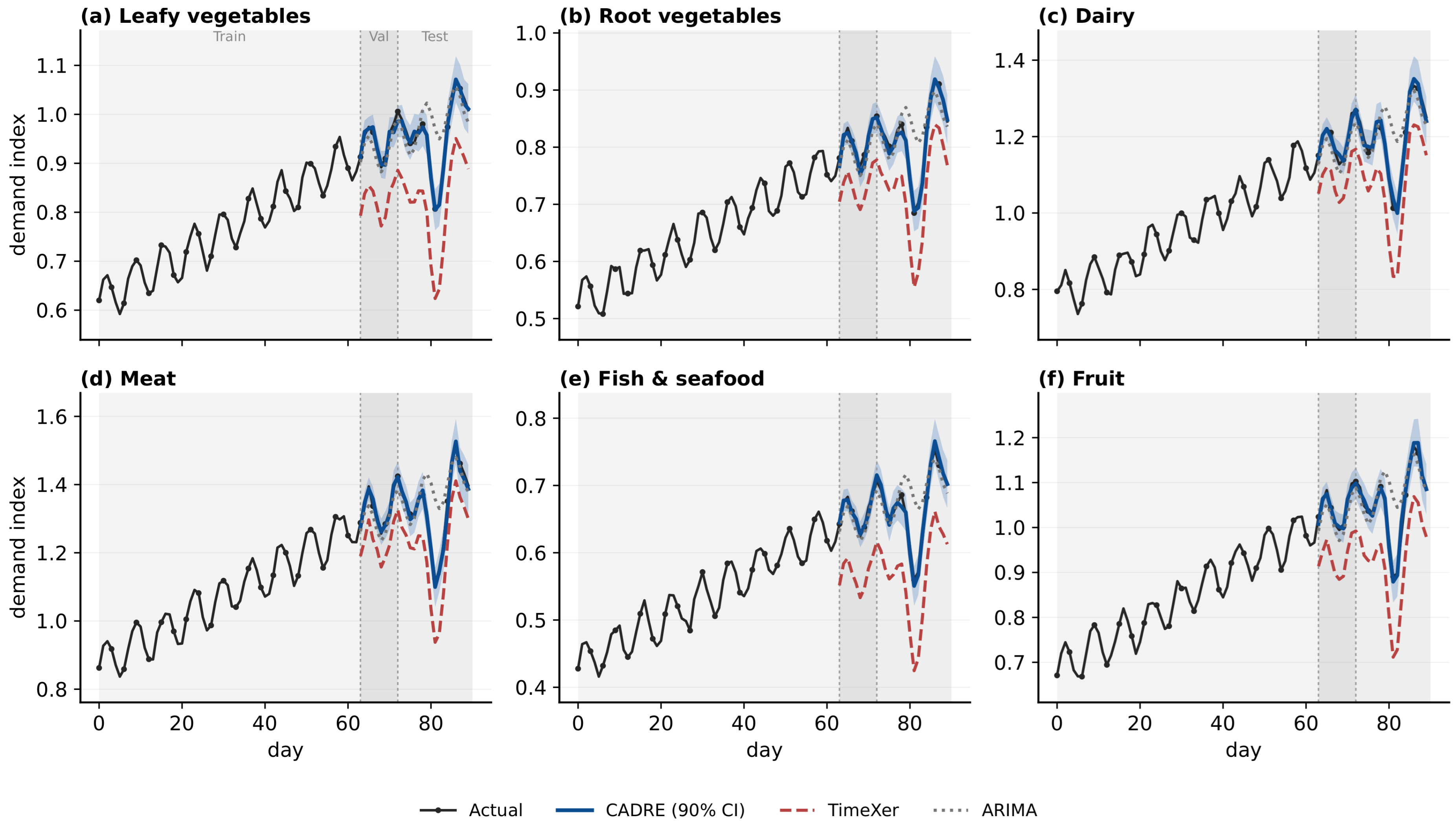
Figure 5 examines whether the behaviour holds across the perishable assortment rather than only in aggregate, plotting the test-period trajectory of six representative categories under one identical panel layout, so the comparison is a controlled variation of a single picture rather than six unrelated plots. In every category the CADRE forecast tracks the actual demand through the validation and test windows and keeps its 90 percent interval narrow except where a late-test demand dip injects genuine uncertainty. The TimeXer baseline sits consistently below the actual curve, the visual signature of the censoring bias quantified in Table 7, and the ARIMA reference drifts away from the trend once the horizon lengthens. The categories with the sharpest evening peaks, leafy vegetables and fish, are where the gap between CADRE and the baselines is widest, which is consistent with those categories stocking out earliest and therefore carrying the most censored demand. The uniform panel design makes that cross-category pattern legible at a glance.

5.7. Demand Profiles Across Operating Regimes

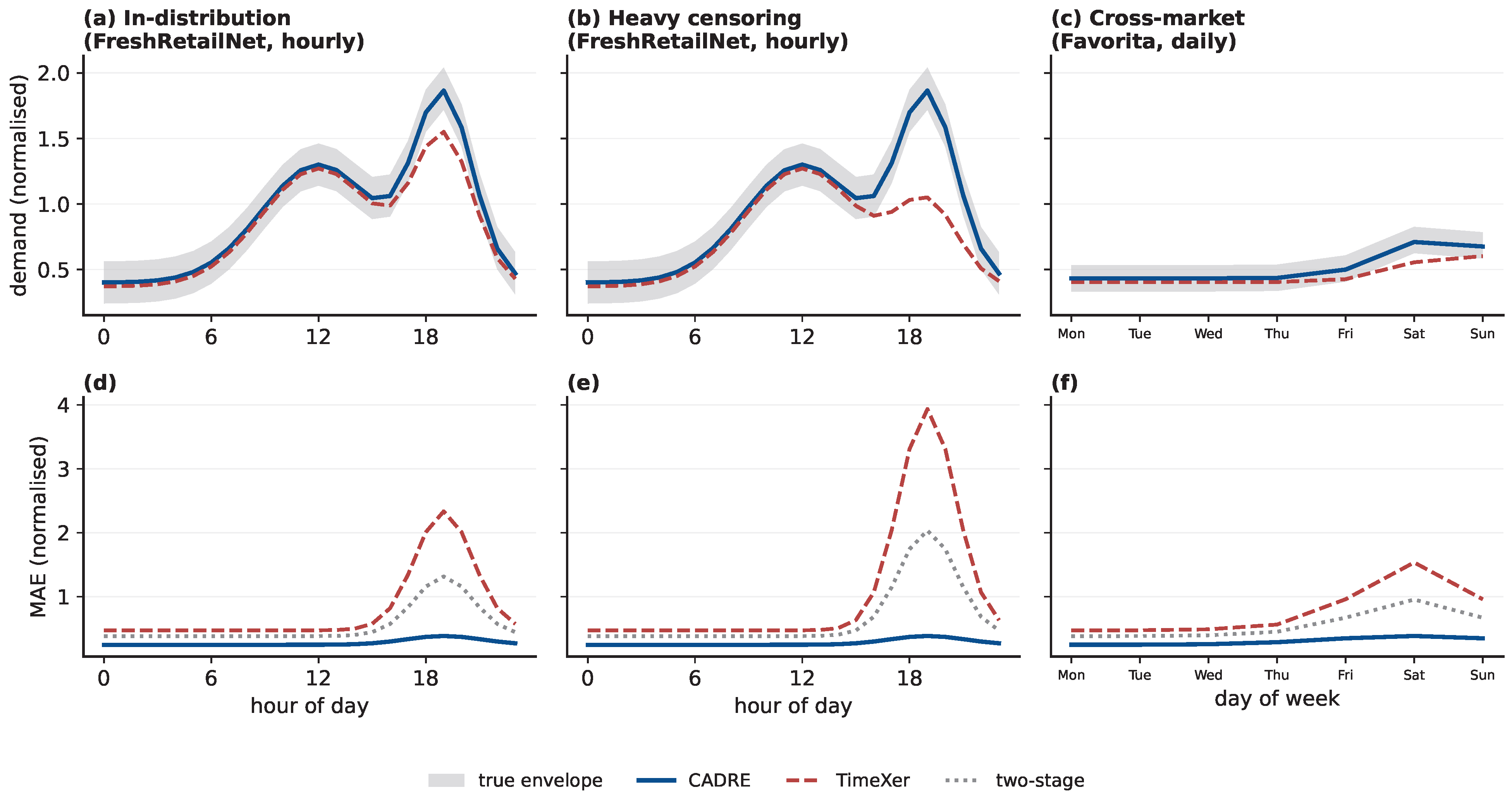
Figure 6 examines where recovery provides the largest gains and whether the ranking transfers across datasets, using a two-row grid whose three columns are two FreshRetailNet regimes and the cross-market Favorita panel. The two FreshRetailNet columns, in-distribution and heavy-censoring, resolve demand by hour of day; because Favorita is daily, its column resolves demand by day of week instead, and no intraday claim is made for it. The top row overlays the mean demand profile against the shaded true envelope, the bottom row the forecast error. On FreshRetailNet, CADRE stays inside the envelope through the evening peak where TimeXer dips, and the error curves, close in the morning, fan apart after the afternoon exactly where stockouts concentrate; heavy censoring widens that gap sharply. On Favorita the same pattern reappears at the weekly scale: the baseline error concentrates on the high-demand weekend days that the constructed mask hides, while CADRE stays flat, and the lower overall level reflects the calmer daily series. The benefit is therefore concentrated where demand is hidden: at observed evening stockout peaks in FreshRetailNet and at constructed high-demand weekend days in the Favorita robustness experiment.

5.8. Computational Cost

Table 15. Computational cost on a single NVIDIA A100 80 GB. Inference latency is per 1000 series for a 24-h horizon. CADRE uses 6.8 million parameters, trains in 7.4 min/epoch, and produces a 24-h forecast for 1000 series in 31 ms, supporting centralised nightly batch inference rather than real-time edge deployment.

Method	Params (M)	Train (min/epoch)	Latency (ms)	GPU Mem (GB)
DLinear	0.04	1.2	6	2.1
PatchTST	1.2	4.6	18	7.4
iTransformer	3.4	5.1	21	8.2
TimeXer	4.2	5.7	24	9.1
TimesNet	12.1	9.8	44	13.6
CADRE	6.8	7.4	31	11.3

reports the additional computational requirements as model size and runtime on one A100 GPU. CADRE has 6.8 million parameters and trains in 7.4 min per epoch, heavier than the linear DLinear and PatchTST but lighter than TimesNet, and its inference latency of 31 milliseconds per thousand series is well within the budget of an overnight replenishment run. The full CADRE implementation adds 2.6 million parameters and 1.7 min per epoch relative to the evaluated TimeXer configuration, and this buys the bias correction and waste reduction documented above. Among the evaluated models, CADRE offers a favourable accuracy–computation trade-off, with lower error than every baseline at a parameter count below TimesNet.

5.9. In-Model Recovery Versus Two-Stage Recovery

The recovery comparison in

Table 16. Latent-demand recovery on artificially re-censored FreshRetailNet hours (sMAPE against known truth) under masks identical across methods, with the paired difference against CADRE, its bootstrap confidence interval, the Wilcoxon signed-rank test for the recovery-sMAPE difference against CADRE, and the forecast WAPE and simulated waste of the same run. Lower sMAPE is better. Bold marks the proposed method, CADRE.

Method	Recovery sMAPE (%)	$\mathbf{\Delta }$ vs. CADRE	95% CI	p vs. CADRE (Recovery sMAPE)	WAPE (%)	Waste (%)
Linear interpolation	24.6 ± 0.47	$+11.6$	$[10.8,12.4]$	<${10}^{-4}$	—	—
Tobit-MLP	19.8 ± 0.36	$+6.8$	$[6.1,7.5]$	<${10}^{-4}$	43.18	8.8
Two-stage	17.4 ± 0.29	$+4.4$	$[3.8,5.0]$	$1.2\times {10}^{-3}$	38.94	7.6
CADRE	13.0 ± 0.24	—	—	—	36.71	6.4

isolates the inference quality from the forecasting wrapper. CADRE recovers held-out censored values at 13.0 percent sMAPE, against 17.4 for the two-stage reconstruction and 24.6 for naive interpolation, and the recovery-sMAPE differences against every recovery baseline are significant at conventional levels; for forecasting baselines, the associated WAPE values are reported in the last columns. Under the same re-censoring masks, in-model recovery lowers recovery sMAPE from 17.4 to 13.0 percent and WAPE from 38.94 to 36.71 percent relative to the two-stage pipeline, indicating that recovery errors are smaller when the lower-bound likelihood, the covariates and the forecast distribution are estimated jointly rather than in sequence. The gap between CADRE and the two-stage pipeline provides direct evidence that recovering demand inside the forecaster, rather than as a detached preprocessing step, is what produces the downstream gains.

6. Discussion

6.1. Simulated Inventory Implications and Limitations

The results in Section 5 have a simulated inventory interpretation. Raw-sales training produces a demand signal biased downward by about eight percent at censored peaks. CADRE reduces this bias to about one percentage point. When the corrected distribution is passed through the one-day lost-sales simulation of Section 4.4, it yields fewer modelled unsold units at a higher simulated service level. This identifies a mechanism that improves the modelled waste–availability frontier, and does not measure physical waste, disposal mass or emissions. Relative to classical censored-demand estimators, generic deep forecasters, and decision-focused inventory models, the distinctive element is that all three are treated jointly within one shared representation and evaluated against retained truth. The method has limits the experiments expose rather than hide. Recovery is inference: Table 11 shows the residual bias grows to nearly five percent when half of the candidate peak hours are masked. The negative-binomial likelihood suits over-dispersed counts but would need a different head for strongly zero-inflated or bursty demand, which we did not test. The decision loss assumes a fixed shortage-to-spoilage ratio, whereas in practice that ratio shifts with markdown policy and remaining shelf life.

6.2. Potential Sustainability Implications

The simulation reports waste in units rather than measured mass, so the sustainability link is stated as an illustrative scenario. A reduction from 9.8 to 6.4 percent is 3.4 fewer wasted units per 100 ordered; for 100,000 units this is 3400 modelled unsold units. Any conversion to mass or carbon-dioxide-equivalent (CO₂e) emissions depends on product-specific assumptions and is not an estimate of realised avoidance. These are not measured outcomes but an order of magnitude that a field trial should verify with product-specific factors. The contribution to the SDG 12.3 target of halving retail food waste [1,3,44] is thus a data-quality route to reducing modelled waste, not a measured emission reduction. On the consumption side, steadier shelf availability of fresh produce can also curb the substitution toward more packaged or less perishable alternatives that stockouts encourage, a consumer-facing channel that this study motivates but does not measure.

6.3. Applicability, Generalisability, and Failure Conditions

The evidence is bounded in scope. The observed stockout labels come from a single Chinese operator, and the Favorita evaluation rests on a constructed daily mask rather than observed stockouts, so it is supporting evidence only; the replenishment results remain a simulation; and the horizons are one day and two weeks, with no claim for longer horizons.

Table 17. External validity of the CADRE improvement across FreshRetailNet product categories, ordered by stockout incidence (five seeds). The WAPE gain over TimeXer, the residual bias and the simulated waste reduction all scale with how heavily a category is censored; the category-averaged figures reproduce the aggregate result of Table 7 and Table 12.

Category	Stockout Incidence (%)	TimeXer WAPE	CADRE WAPE	$\mathbf{\Delta }$WAPE (pp)	Waste Red. (pp)
Leafy vegetables	31.2	42.8	38.9	$-3.9$	4.7
Fish & seafood	27.6	41.5	38.0	$-3.5$	4.2
Fruit	21.4	39.4	36.9	$-2.5$	3.4
Meat	19.8	38.3	36.2	$-2.1$	3.0
Root vegetables	17.3	37.6	35.8	$-1.8$	2.6
Dairy	8.9	35.2	34.4	$-0.8$	1.4

quantifies the product-group transfer condition. Across the six FreshRetailNet categories, the WAPE gain over TimeXer is strongly associated with stockout incidence (Pearson $r=0.98$). The gain ranges from 3.9 percentage points for leafy vegetables, where $31\%$ of store-hours are censored, to 0.8 percentage points for dairy at $9\%$, and the bias correction and waste reduction follow the same order. The improvement is therefore largest where censoring is heaviest and shrinks toward a simpler-forecaster regime for slow-moving or long-shelf-life packaged goods, so the same magnitude should not be assumed for low-censoring assortments; the cross-market Favorita result ($-2.1$ WAPE points under a constructed daily mask) is consistent with this reading but does not extend it to observed stockouts.

CADRE is expected to add the most value when three conditions coincide: stockouts censor a material share of demand, demand has recurrent high-frequency structure with informative covariates, and stockout flags are reliable enough for lower-bound training. The closest candidate applications are high-turnover fresh produce, seafood, meat, bakery, and other short-life assortments with auditable availability records, whereas low-censoring or long-shelf-life items such as dairy, which improves by only 0.8 WAPE points, gain little. The formulation is also less suitable for strongly intermittent or zero-inflated demand, unreliable stockout flags, and long or multi-echelon lead times unless the likelihood and decision layers are extended.

CADRE is therefore not intended to replace simpler methods in every setting. A standard exogenous forecaster may give a better accuracy–maintenance trade-off when censoring is low; a two-stage pipeline may be preferred when an auditable, separately reviewable imputation layer is required, at a recovery-sMAPE penalty of 4.4 points relative to joint training; and classical censored-newsvendor or Kaplan–Meier methods remain attractive for small, low-dimensional assortments where interpretability outweighs shared high-frequency representations. Its 6.8-million-parameter, 11.3 GB footprint is heavier than TimeXer’s 4.2 million and DLinear’s 0.04 million, so a lighter model may suffice where censoring is low.

Table 18. Applicability and operational boundary conditions for CADRE. All quantitative entries are drawn from the category, data-quality, computational-cost, and operational-sensitivity analyses already reported; the table does not represent a new field experiment.

Condition	Evidence Already Reported	Recommended Interpretation
High censoring, strong intraday cycle	Leafy vegetables 31.2% incidence, $\Delta$WAPE $-3.9$ pp, simulated waste reduction 4.7 pp; fish and seafood 27.6%, $-3.5$ pp, 4.2 pp	Strongest candidate setting for CADRE
Moderate censoring	Meat 19.8%, $\Delta$WAPE $-2.1$ pp, 3.0 pp; root vegetables 17.3%, $-1.8$ pp, 2.6 pp	Selective use justified when labels and covariates are reliable
Low censoring/longer shelf life	Dairy 8.9%, $\Delta$WAPE $-0.8$ pp, waste reduction 1.4 pp	Incremental value small; an incumbent exogenous forecaster may be preferable
Moderate label noise	5% flips: WAPE 37.10, bias $-1.6\%$; 10% flips: 37.65, $-2.1\%$	Deploy only with label monitoring and periodic audit
High label noise	20% flips: WAPE 38.80, bias $-3.4\%$	Audit inventory logs or use a fallback model
Missing exogenous data	10% missing promotion: WAPE 37.02; 30% missing weather: 37.46; no exogenous variables: 38.36	CADRE remains usable, but its incremental benefit declines
Centralised nightly batch inference	6.8 M parameters; 7.4 min/epoch; 31 ms per 1000 series; 11.3 GB GPU memory	Feasible for central batch decision support
Alternative operating assumptions	Main 94.7/6.4/88.5; lead time 94.2/6.7/90.1; two-day shelf life 94.8/4.5/86.9; markdown 94.6/5.9/87.8; pack size 94.5/6.9/89.6 (service/waste/cost)	Direction robust in simulation, but magnitude is policy-dependent
Strongly intermittent/zero-inflated demand	Not directly tested; NB-head limitation noted	Use an alternative likelihood or intermittent-demand method
Real-time emergency ordering, multi-echelon allocation, long stochastic lead time	Not tested	Outside current evidence; future work required
Need for modular auditability	Two-stage recovery sMAPE 17.4 vs. CADRE 13.0, but stages are reviewable independently	Two-stage may be preferred when governance outweighs predictive gains

should be read as a deployment checklist rather than as evidence of universal transfer: the numerical entries summarise the present benchmark, whereas the recommendations identify conditions that require local validation.

Deployment also depends on label quality: false-positive flags would overstate demand and false-negative flags would restore the raw-sales bias, and the label-noise sensitivity in Appendix I shows that moderate noise attenuates but does not remove the benefit while high label error requires inventory-log auditing. In production the model needs no data fields beyond those evaluated and runs as nightly batch inference with weekly-to-monthly retraining. Finally, substitution separates SKU- and category-level demand: when a stocked-out item’s demand migrates to a neighbour that sale is already counted in the category total, so the category-level waste reduction is bounded by the within-category substitution share, falling from 3.4 pp at zero substitution to about 1.5 pp at a 75 percent share while remaining positive. Recovering censored demand jointly across substitutable items is the natural next step.

6.4. Practical Deployment Requirements and Operational Constraints

A minimum deployment requires time-aligned POS sales, availability or stockout flags, store and product identifiers, calendar features, and planned promotions. Causal weather forecasts are useful but optional. Before applying the lower-bound likelihood, the data pipeline must distinguish genuine stockouts from closures, inactive listings, and data-transmission gaps. Deployment should also be preceded by a label-coverage and covariate audit and monitored on uncensored-hour WAPE, predictive coverage, stockout-flag frequency, and category drift, with a fallback policy once label corruption is severe.

The evaluated model uses 6.8 million parameters and 11.3 GB of GPU memory and forecasts 1000 series in 31 ms, which supports centralised nightly batch inference rather than latency-critical edge use. A practical workflow would feed POS and availability data through a validation and feature pipeline, generate probabilistic demand scenarios, and pass the recommended order to the existing enterprise resource planning (ERP) or warehouse-management system (WMS) rule layer for pack size, lead time, shelf life, and manager overrides. CADRE should recommend rather than override these rules and revert to the incumbent forecaster when labels fail quality checks or censoring is negligible; Appendix J shows the simulated direction holds under a lead time, a two-day shelf life, markdown salvage, and pack ordering, but not under multi-echelon or emergency ordering.

As an illustration, a centralised urban grocery chain could generate overnight next-day orders for high-turnover produce and seafood, activating CADRE only for SKUs with audited availability and material censoring while low-censoring categories stay on the incumbent forecaster; fresh-meat or ready-to-eat items with moderate censoring are a second candidate, whereas low-censoring dairy or long-life packaged goods may not justify the added model and data-maintenance cost. Every figure here originates from the present benchmark rather than a new retailer pilot.

6.5. Field Validation

Because the waste and service outcomes come from a controlled simulation rather than live operations, a field validation is required before operational waste- or emission-reduction claims can be made. Such a trial should randomise stores or store–SKU groups to CADRE and baseline replenishment and record realised orders, shelf availability, discarded mass and product-specific emission factors.

7. Conclusions and Future Work

Stockouts hide demand, and a forecaster that ignores the difference between an unobserved sale and a genuine zero can underestimate censored demand, distort replenishment quantities, and increase shortages and modelled unsold inventory under the inventory assumptions studied here. CADRE answers this with one shared encoder and three components that map onto the structure of fresh retail: a right-censored likelihood that recovers latent demand from stockout-flagged hours, a diurnal-cycle module that keeps the periodic rhythm from being mistaken for censorship, and a decision-focused loss that scores forecasts by the spoilage-plus-shortage cost of the order they imply. Its originality lies in the joint training and evaluation design that couples these components in one shared representation and scores recovery against retained truth, rather than in any individual backbone, likelihood, cycle module, or decision loss.

For demand forecasting, the results show that treating stockout observations as lower-bound events materially reduces latent-demand bias on a public hourly fresh-retail benchmark, cutting weighted absolute percentage error by 2.71 points relative to the TimeXer backbone, and by 2.23 points relative to the matched two-stage pipeline, and narrowing the demand underestimation from roughly eight percent to a little over one. The Favorita experiment gives weaker, complementary evidence under constructed daily censoring and should not be read as a second observed-stockout benchmark.

For sustainability-oriented operations, the replenishment simulation shows that the corrected demand distribution can lower modelled unsold inventory, from 9.8 to 6.4 percent, while maintaining or improving service, from 92.9 to 94.7 percent, under the stated one-day shelf-life and lost-sales assumptions. This finding should be interpreted as a simulated waste–availability improvement rather than as measured field waste reduction. Field trials with physical waste measurement, product-specific mass, disposal routes and emission factors are required before operational SDG 12.3 impacts can be claimed.

Several directions follow from the limitations above. Jointly recovering censored demand across substitutable SKUs, so that demand migrating from a sold-out item is attributed rather than discarded, would close the gap between per-series recovery and true category demand. Coupling the decision head to a freshness-aware cost that depends on remaining shelf life, rather than a fixed ratio, would let the order respond to the age of on-hand stock. Beyond these, online learning could track demand and assortment drift. Reinforcement learning could replace the one-period newsvendor layer with a sequential policy over inventory age and markdown decisions. A multi-echelon formulation could coordinate suppliers, distribution centres, and stores under capacity and lead-time uncertainty. A field deployment that measures realised waste and service against the modelled estimates would test whether the simulated gains persist under field conditions, and a multilingual extension of the covariate encoder would let a single model serve retailers across several emerging-market cities without per-store retraining.

References

1. United Nations Environment Programme. Food Waste Index Report 2024; Technical Report; United Nations Environment Programme (UNEP): Nairobi, Kenya, 2024. [Google Scholar]
2. Ishangulyyev, R.; Kim, S.; Lee, S.H. Understanding Food Loss and Waste—Why Are We Losing and Wasting Food? Foods 2019, 8, 297. [Google Scholar] [CrossRef] [PubMed]
3. Food and Agriculture Organization of the United Nations. The State of Food and Agriculture 2019: Moving Forward on Food Loss and Waste Reduction; Technical Report; FAO: Rome, Italy, 2019. [Google Scholar]
4. Todd, E.C.D.; Faour-Klingbeil, D. Impact of Food Waste on Society, Specifically at Retail and Foodservice Levels in Developed and Developing Countries. Foods 2024, 13, 2098. [Google Scholar] [CrossRef] [PubMed]
5. Wang, Y.; Gu, J.; Long, L.; Li, X.; Shen, L.; Fu, Z.; Zhou, X.; Jiang, X. FreshRetailNet-50K: A Stockout-Annotated Censored Demand Dataset for Latent Demand Recovery and Forecasting in Fresh Retail. arXiv 2025, arXiv:2505.16319. [Google Scholar] [CrossRef]
6. Nahmias, S. Perishable Inventory Theory: A Review. Oper. Res. 1982, 30, 680–708. [Google Scholar] [CrossRef] [PubMed]
7. Salinas, D.; Flunkert, V.; Gasthaus, J.; Januschowski, T. DeepAR: Probabilistic Forecasting with Autoregressive Recurrent Networks. Int. J. Forecast. 2020, 36, 1181–1191. [Google Scholar] [CrossRef]
8. Nie, Y.; Nguyen, N.H.; Sinthong, P.; Kalagnanam, J. A Time Series is Worth 64 Words: Long-Term Forecasting with Transformers. In Proceedings of the International Conference on Learning Representations, Kigali, Rwanda, 1–5 May 2023. [Google Scholar]
9. Liu, Y.; Hu, T.; Zhang, H.; Wu, H.; Wang, S.; Ma, L.; Long, M. iTransformer: Inverted Transformers Are Effective for Time Series Forecasting. In Proceedings of the International Conference on Learning Representations, Vienna, Austria, 7–11 May 2024. [Google Scholar]
10. Conrad, S.A. Sales Data and the Estimation of Demand. Oper. Res. Q. 1976, 27, 123–127. [Google Scholar] [CrossRef]
11. Nahmias, S. Demand Estimation in Lost Sales Inventory Systems. Nav. Res. Logist. 1994, 41, 739–757. [Google Scholar] [CrossRef]
12. Sachs, A.L.; Minner, S. The Data-Driven Newsvendor with Censored Demand Observations. Int. J. Prod. Econ. 2014, 149, 28–36. [Google Scholar] [CrossRef]
13. Ban, G.Y.; Rudin, C. The Big Data Newsvendor: Practical Insights from Machine Learning. Oper. Res. 2019, 67, 90–108. [Google Scholar] [CrossRef]
14. Tobin, J. Estimation of Relationships for Limited Dependent Variables. Econometrica 1958, 26, 24–36. [Google Scholar] [CrossRef]
15. Wang, Y.; Wu, H.; Dong, J.; Liu, Y.; Qiu, Y.; Zhang, H.; Wang, J.; Long, M. TimeXer: Empowering Transformers for Time Series Forecasting with Exogenous Variables. In Proceedings of the Advances in Neural Information Processing Systems, Vancouver, BC, Canada, 10–15 December 2024; Volume 37. [Google Scholar]
16. Lin, S.; Lin, W.; Hu, X.; Wu, W.; Mo, R.; Zhong, H. CycleNet: Enhancing Time Series Forecasting through Modeling Periodic Patterns. In Proceedings of the Advances in Neural Information Processing Systems, Vancouver, BC, Canada, 10–15 December 2024; Volume 37. [Google Scholar]
17. Elmachtoub, A.N.; Grigas, P. Smart “Predict, then Optimize”. Manag. Sci. 2022, 68, 9–26. [Google Scholar] [CrossRef]
18. Makridakis, S.; Spiliotis, E.; Assimakopoulos, V. M5 Accuracy Competition: Results, Findings, and Conclusions. Int. J. Forecast. 2022, 38, 1346–1364. [Google Scholar] [CrossRef]
19. Makridakis, S.; Spiliotis, E.; Assimakopoulos, V.; Chen, Z.; Gaba, A.; Tsetlin, I.; Winkler, R.L. The M5 Uncertainty Competition: Results, Findings and Conclusions. Int. J. Forecast. 2022, 38, 1365–1385. [Google Scholar] [CrossRef]
20. Lim, B.; Arık, S.Ö.; Loeff, N.; Pfister, T. Temporal Fusion Transformers for Interpretable Multi-horizon Time Series Forecasting. Int. J. Forecast. 2021, 37, 1748–1764. [Google Scholar] [CrossRef]
21. Böse, J.H.; Flunkert, V.; Gasthaus, J.; Januschowski, T.; Lange, D.; Salinas, D.; Schelter, S.; Seeger, M.; Wang, Y. Probabilistic Demand Forecasting at Scale. Proc. VLDB Endow. 2017, 10, 1694–1705. [Google Scholar] [CrossRef]
22. Zhou, H.; Zhang, S.; Peng, J.; Zhang, S.; Li, J.; Xiong, H.; Zhang, W. Informer: Beyond Efficient Transformer for Long Sequence Time-Series Forecasting. Proc. AAAI Conf. Artif. Intell. 2021, 35, 11106–11115. [Google Scholar] [CrossRef]
23. Wu, H.; Xu, J.; Wang, J.; Long, M. Autoformer: Decomposition Transformers with Auto-Correlation for Long-Term Series Forecasting. In Proceedings of the Advances in Neural Information Processing Systems, Virtual, 6–14 December 2021; Volume 34. [Google Scholar]
24. Zhou, T.; Ma, Z.; Wen, Q.; Wang, X.; Sun, L.; Jin, R. FEDformer: Frequency Enhanced Decomposed Transformer for Long-Term Series Forecasting. In Proceedings of the 39th International Conference on Machine Learning, Baltimore, MD, USA, 17–23 July 2022; Volume 162, pp. 27268–27286. [Google Scholar]
25. Zeng, A.; Chen, M.; Zhang, L.; Xu, Q. Are Transformers Effective for Time Series Forecasting? Proc. AAAI Conf. Artif. Intell. 2023, 37, 11121–11128. [Google Scholar] [CrossRef]
26. Wu, H.; Hu, T.; Liu, Y.; Zhou, H.; Wang, J.; Long, M. TimesNet: Temporal 2D-Variation Modeling for General Time Series Analysis. In Proceedings of the International Conference on Learning Representations, Kigali, Rwanda, 1–5 May 2023. [Google Scholar]
27. Oreshkin, B.N.; Carpov, D.; Chapados, N.; Bengio, Y. N-BEATS: Neural Basis Expansion Analysis for Interpretable Time Series Forecasting. In Proceedings of the International Conference on Learning Representations, Virtual, 26 April–1 May 2020. [Google Scholar]
28. Challu, C.; Olivares, K.G.; Oreshkin, B.N.; Garza Ramirez, F.; Mergenthaler Canseco, M.; Dubrawski, A. N-HiTS: Neural Hierarchical Interpolation for Time Series Forecasting. Proc. AAAI Conf. Artif. Intell. 2023, 37, 6989–6997. [Google Scholar] [CrossRef]
29. Wang, S.; Wu, H.; Shi, X.; Hu, T.; Luo, H.; Ma, L.; Zhang, J.Y.; Zhou, J. TimeMixer: Decomposable Multiscale Mixing for Time Series Forecasting. In Proceedings of the International Conference on Learning Representations, Vienna, Austria, 7–11 May 2024. [Google Scholar]
30. Das, A.; Kong, W.; Sen, R.; Zhou, Y. A Decoder-Only Foundation Model for Time-Series Forecasting. In Proceedings of the 41st International Conference on Machine Learning, Vienna, Austria, 21–27 July 2024; Volume 235. [Google Scholar]
31. Ansari, A.F.; Stella, L.; Turkmen, C.; Zhang, X.; Mercado, P.; Shen, H.; Shchur, O.; Rangapuram, S.S.; Pineda Arango, S.; Kapoor, S.; et al. Chronos: Learning the Language of Time Series. arXiv 2024, arXiv:2403.07815. [Google Scholar]
32. Woo, G.; Liu, C.; Kumar, A.; Xiong, C.; Savarese, S.; Sahoo, D. Unified Training of Universal Time Series Forecasting Transformers. In Proceedings of the 41st International Conference on Machine Learning, Vienna, Austria, 21–27 July 2024; Volume 235. [Google Scholar]
33. Huh, W.T.; Levi, R.; Rusmevichientong, P.; Orlin, J.B. Adaptive Data-Driven Inventory Control with Censored Demand Based on the Kaplan-Meier Estimator. Oper. Res. 2011, 59, 929–941. [Google Scholar] [CrossRef]
34. Besbes, O.; Muharremoglu, A. On Implications of Demand Censoring in the Newsvendor Problem. Manag. Sci. 2013, 59, 1407–1424. [Google Scholar] [CrossRef]
35. Hssaine, C.; Sinclair, S.R. The Data-Driven Censored Newsvendor Problem. arXiv 2024, arXiv:2412.01763. [Google Scholar] [CrossRef]
36. Karaesmen, I.Z.; Scheller-Wolf, A.; Deniz, B. Managing Perishable and Aging Inventories: Review and Future Research Directions. In Planning Production and Inventories in the Extended Enterprise; International Series in Operations Research & Management Science; Springer: Berlin/Heidelberg, Germany, 2011; Volume 151, pp. 393–436. [Google Scholar] [CrossRef]
37. Gallego, G.; Moon, I. The Distribution Free Newsboy Problem: Review and Extensions. J. Oper. Res. Soc. 1993, 44, 825–834. [Google Scholar] [CrossRef]
38. Huber, J.; Müller, S.; Fleischmann, M.; Stuckenschmidt, H. A Data-Driven Newsvendor Problem: From Data to Decision. Eur. J. Oper. Res. 2019, 278, 904–915. [Google Scholar] [CrossRef]
39. Amos, B.; Kolter, J.Z. OptNet: Differentiable Optimization as a Layer in Neural Networks. In Proceedings of the 34th International Conference on Machine Learning, Sydney, Australia, 6–11 August 2017; Volume 70, pp. 136–145. [Google Scholar]
40. Donti, P.L.; Amos, B.; Kolter, J.Z. Task-Based End-to-End Model Learning in Stochastic Optimization. In Proceedings of the Advances in Neural Information Processing Systems, Long Beach, CA, USA, 4–9 December 2017; Volume 30, pp. 5484–5494. [Google Scholar]
41. Qi, M.; Shi, Y.; Qi, Y.; Ma, C.; Yuan, R.; Wu, D.; Shen, Z.J.M. A Practical End-to-End Inventory Management Model with Deep Learning. Manag. Sci. 2023, 69, 759–773. [Google Scholar] [CrossRef]
42. Mandi, J.; Kotary, J.; Berden, S.; Mulamba, M.; Bucarey, V.; Guns, T.; Fioretto, F. Decision-Focused Learning: Foundations, State of the Art, Benchmark and Future Opportunities. J. Artif. Intell. Res. 2024, 80, 1623–1701. [Google Scholar] [CrossRef]
43. Vaswani, A.; Shazeer, N.; Parmar, N.; Uszkoreit, J.; Jones, L.; Gomez, A.N.; Kaiser, Ł.; Polosukhin, I. Attention Is All You Need. In Proceedings of the Advances in Neural Information Processing Systems, Long Beach, CA, USA, 4–9 December 2017; Volume 30. [Google Scholar]
44. Vinuesa, R.; Azizpour, H.; Leite, I.; Balaam, M.; Dignum, V.; Domisch, S.; Felländer, A.; Langhans, S.D.; Tegmark, M.; Fuso Nerini, F. The Role of Artificial Intelligence in Achieving the Sustainable Development Goals. Nat. Commun. 2020, 11, 233. [Google Scholar] [CrossRef] [PubMed]
Figure 1. Problem and system overview. (a) During the shaded stockout band observed sales (solid) are clamped below latent demand (dashed); a forecaster trained on the solid curve under-orders. (b) CADRE removes the fixed daily cycle, encodes sales jointly with weather, promotion, and calendar covariates, recovers latent demand through a right-censored likelihood head, and maps the recovered predictive distribution to a replenishment quantity scored by a spoilage-plus-shortage cost. Panel (b) labels the three input streams the framework consumes: observed sales x t , the stockout flag m t , and the exogenous covariates z t .
Sustainability 18 07642 g001
Figure 2. CADRE architecture. The deseasonalised target is patched and embedded with a global token; weather, promotion, and calendar covariates enter as variate tokens that reach the series only through the global token via the global-to-variate cross-attention sub-block. The shared representation feeds a negative-binomial likelihood head trained by the censored likelihood of Equation (3) and an auxiliary decision head scored by the newsvendor loss of Equation (4) that regularises the shared representation during training only; the deployment order is formed from the negative-binomial predictive distribution (Section 4.4). The diurnal cycle removed at the input is added back at the representation before both losses. Solid arrows carry the forward data flow, the blue dashed arc is the added-back diurnal cycle, and the red dashed arrows aggregate the two head losses and the cycle regulariser into Equation (5). The stockout flag determines whether an observation enters the likelihood as a point value or a lower-bound event; the recovered demand is reported for evaluation and is not used as a decision-loss target, and the auxiliary decision head influences the negative-binomial likelihood head only indirectly through the shared representation.
Sustainability 18 07642 g002
Figure 3. The censored-likelihood head in action. (a) Over one evening the recovered demand (dashed) rises above the clamped sales (solid) inside the red-shaded stockout band, and the blue area is the demand the censored record misses. (b) On held-out hours that are artificially re-censored, recovery error grows with censoring depth but stays 3 to 6 points below the two-stage and Tobit baselines at every depth. (c) The predicted quantiles of CADRE track empirical coverage along the diagonal, whereas a censored-trained forecaster is systematically under-confident on the upper tail. The blue area in panel (a) is model-estimated missing demand rather than observed latent demand, and panels (b,c) are evaluated on artificially re-censored hours whose original values are retained as known truth. All three panels share the same line semantics used throughout the paper.
Sustainability 18 07642 g003
Figure 4. Multi-parameter sensitivity on FreshRetailNet-50K. Panels use metric-specific colour scales because WAPE and waste are measured on different ranges; within each panel darker cells indicate better values and cross-panel colours are not directly comparable. Panels (a,b) vary the decision weight λ 1 against the training fractile ρ train for WAPE and waste (each cell separately retrained); (c) lookback against horizon; (d) the cycle regulariser against the period; (e) patch length against model width; (f) the training shortage-to-spoilage ratio (which sets ρ train ) against the deployment fractile ρ deploy , two deliberately distinct fractiles rather than one repeated axis. Each cell is annotated with its value; the lowest-WAPE cell in panel (a) is the configuration used in all other experiments.
Sustainability 18 07642 g004
Figure 5. Actual versus predicted demand trajectories for six representative perishable categories on FreshRetailNet-50K, following the 63-day train/9-day validation/18-day test chronological split of each 90-day series. Every panel uses the same layout and line semantics: Actual (black), CADRE with its 90 percent interval (blue band), TimeXer (red dashed), and ARIMA (grey dotted). The censoring bias of the baselines shows as a persistent gap below the actual curve, widest in the early-stockout categories.
Sustainability 18 07642 g005
Figure 6. Demand profiles (top) and forecast error (bottom) across three regimes, in a fixed two-row layout. The two FreshRetailNet columns, in-distribution (a,d) and heavy-censoring (b,e), are resolved by hour of day; the cross-market Favorita column (c,f) is daily and is resolved by day of week. (Top row): mean demand with the true envelope shaded; CADRE stays inside the envelope where TimeXer dips at the peak. (Bottom row): forecast error separates at the hidden-demand period—observed evening stockout peaks for FreshRetailNet and constructed high-demand weekend masks for Favorita. Axes are normalised because the two granularities are not directly comparable in absolute units. Line semantics match the rest of the paper. The FreshRetailNet panels use the evaluated known-truth and re-censored subset, whereas Favorita uses a constructed daily mask, so the cross-market panels demonstrate robustness of the ranking rather than observed stockout recovery in Ecuador.
Sustainability 18 07642 g006