Article

Compound Drought Identification and Driving Force Analysis in the Chushandian Irrigation Area Based on a Copula Function

1
Henan Chushandian Reservoir Irrigation Project Co., Ltd., Xinyang 464043, China
2
China Institute of Water Resources and Hydropower Research, Beijing 100080, China
3
School of Water Conservancy, North China University of Water Resources and Electric Power, Zhengzhou 450046, China
*
Authors to whom correspondence should be addressed.
Sustainability 2026, 18(15), 7598; https://doi.org/10.3390/su18157598 (registering DOI)
Submission received: 20 April 2026 / Revised: 3 July 2026 / Accepted: 23 July 2026 / Published: 26 July 2026
(This article belongs to the Section Sustainable Agriculture)

Abstract

The Chushandian Irrigation Area (CSDIA) lacks a comprehensive drought index integrating meteorological and hydrological information, hindering accurate drought assessment and sustainable water resource management under changing climatic conditions. To address this, a multivariate standardized drought index (MSDI) based on a Copula function was developed, combining precipitation and runoff. Optimized run theory identified compound drought events, and cross-wavelet power spectrum explored large-scale climate drivers. Results show that MSDI correlates strongly with both the Standardized Precipitation Index (SPI) and Standardized Runoff Index (SRI) (Pearson’s r > 0.75, p < 0.01) at the monthly scale, effectively capturing drought onset, duration, and termination. From 1960 to 2018, 110 compound drought events were identified, characterized by short durations (mean 3.82 months) and low intensities (mean 4.43). The most severe event (August 1960–October 1961, duration 15 months, intensity 22.72) has a return period of about 40 years. Among nine teleconnection factors, ENSO is the dominant driver, followed by sunspot activity (SSI). BEAST change-point detection revealed a shift toward drought intensification after 1990, underscoring the need for adaptive water management strategies. These findings provide scientific support for sustainable drought monitoring, climate-resilient agricultural planning, and adaptive water management in CSDIA, contributing to the broader goal of ensuring food security and water sustainability in monsoon-dependent irrigation systems.

1. Introduction

Drought is a recurring and persistent natural hazard that has intensified in frequency, extent, and severity under global warming [1,2]. The IPCC Sixth Assessment Report projects continued warming and an enhanced hydrological cycle, leading to a higher probability of extreme hydroclimatic events [3]. In China, the monsoon climate results in complex spatiotemporal drought patterns. While northern regions face severe drought conditions, southern China has also experienced increasing drought frequency [4]. Recent extreme events—such as the severe drought in the middle-lower Yangtze River during the summer of 2024 [5] and the spring–summer drought in North China [6]—highlight the urgent need for effective drought monitoring and early warning. Nevertheless, drought formation and evolution are driven by both natural variability and human activities, making their mechanisms complex [7]. Understanding the compound nature of drought and its driving mechanisms is therefore essential for developing sustainable water management strategies that can adapt to accelerating climate change, particularly in agricultural regions where water security underpins food production and rural livelihoods.
Drought indices are fundamental tools for quantifying drought severity and play a critical role in supporting sustainable water resource management by providing early warning signals that enable proactive allocation of limited water supplies. Numerous single indices have been developed for meteorological, hydrological, and agricultural droughts, including the Standardized Precipitation Index (SPI) [8], Standardized Runoff Index (SRI) [9], and Palmer Drought Severity Index (PDSI) [10]. However, single indices typically focus on one type of drought and cannot capture the propagation and co-evolution among different drought types [11]. Recently, composite drought indices that integrate multi-source information have become a research frontier [12].
Existing methods for constructing composite drought indices fall into two categories: weighting or dimension-reduction approaches, and joint distribution methods based on Copula functions. The first category includes techniques such as the Analytic Hierarchy Process (AHP), entropy weighting, and principal component analysis (PCA), which construct composite indices by linearly combining multiple hydrometeorological variables. While widely applied, these methods share inherent limitations: AHP introduces subjectivity through expert-assigned weights; entropy weighting is sensitive to sample characteristics; and PCA seeks directions of maximum variance under linear projections, potentially discarding drought signals from variables that exhibit weak linear associations yet contribute meaningfully to the overall drought state [13]. More fundamentally, these approaches assume that the contribution of each variable is additive and proportional, thereby failing to capture the nonlinear, compound nature of drought, where the joint deficit of multiple variables can produce impacts that exceed the sum of individual deficits.
The second category is grounded in joint distribution theory, where Copula functions have demonstrated exceptional applicability. The theoretical foundation was laid by Sklar [14], who proved that any multivariate joint distribution can be decomposed into its marginal distributions and a Copula function capturing the dependence structure among variables. This is profoundly relevant to drought analysis because hydrometeorological variables such as precipitation and runoff typically follow different marginal distributions (e.g., Gamma, Lognormal, and GEV), yet are coupled through complex, nonlinear dependence mechanisms. Shiau and Modarres [15,16] were among the first to apply Copula-based drought severity–duration–frequency analysis, demonstrating that Copulas could flexibly model the joint behavior of drought characteristics without requiring identical marginal distributions. Kao and Govindaraju [17] subsequently constructed a joint deficit index using Copulas to combine precipitation and runoff, and Hao and AghaKouchak [18] proposed a parametric multivariate standardized drought index (MSDI), which has since become one of the most widely adopted frameworks for compound drought assessment.
The methodological evolution of Copula-based drought indices has continued along several important directions. First, the scope of integrated variables has expanded significantly to include soil moisture, evapotranspiration, groundwater storage, and vegetation indices. For example, Zhao et al. [19] developed an Ecological Comprehensive Drought Index using three-dimensional Copula functions to jointly model multiple ecohydrological variables, while Yu et al. [20] proposed a Copula-based index integrating surface water and groundwater for drought assessment in arid basins. Second, beyond classical Archimedean Copulas, elliptical and nested Copula structures have been explored to better capture asymmetric and tail-dependent relationships [21]; Wang et al. [22] advanced the field with the SPESI index integrating SPEI and SSI through Copula functions. Third, time-varying Copula models have been introduced to address non-stationarity under changing climatic conditions [23], and Copula-based assessments of drought propagation have further broadened the analytical scope. Given these advantages over linear weighting methods—especially in capturing nonlinear dependence and preserving multi-variable drought information—the Copula framework has become the preferred approach for compound drought assessment.
The Chushandian Irrigation Area (CSDIA) is located in the upper Huaihe River Basin in southern Henan Province. It is a large (Type II) irrigation project with a design irrigation area of 527,000 mu (≈35,133 ha). In recent years, frequent short-duration, high-intensity droughts have threatened water supply and agricultural production. For instance, during the 2024 heatwave and drought, the Chushandian Reservoir supplied 81 million m3 of water to support summer sowing. However, no comprehensive drought index integrating both meteorological and hydrological information has been developed for this area, limiting our understanding of drought evolution and its drivers. This gap poses a significant challenge to the sustainable management of water resources in the CSDIA, where agricultural productivity, ecological baseflow maintenance, and domestic water supply must be balanced under increasing climate uncertainty.
Therefore, this study aims to (1) construct a multivariate standardized drought index (MSDI) based on a Copula function that combines precipitation and runoff; (2) characterize the temporal evolution and return periods of compound drought events in CSDIA from 1960 to 2018; (3) detect abrupt changes in MSDI using the Bayesian Estimator of Abrupt change, Seasonal change, and Trend (BEAST) algorithm; and (4) quantify the contributions of large-scale climate drivers via cross-wavelet transform and SHapley Additive exPlanations (SHAP) analysis. The results will provide scientific support for drought monitoring and sustainable water resource management in the study area, contribute to the development of climate-adaptive irrigation strategies that enhance regional water security and food sustainability, and serve as a methodological reference for similar irrigated regions worldwide that face compound drought risks under global warming.

2. Materials and Methods

2.1. Study Area

The Chushandian Irrigation Area (CSDIA) is situated in the upper Huaihe River Basin in southern Henan Province, China (Figure 1). It stretches from downstream of the Chushandian Reservoir in the west to Zhengyang County in the east, and from Shihe District in the south to Queshan County in the north, covering a geographic range of 113°58′–114°35′ E and 32°15′–32°48′ N [24,25]. As a critical component of the upper Huaihe agricultural system, the CSDIA plays a vital role in agricultural irrigation, domestic and industrial water supply, and ecological flow regulation. Frequent drought events in recent decades have severely threatened water availability and agricultural production, highlighting the urgent need to understand the area’s compound drought characteristics and their underlying drivers [26,27].
The Changtaiguan (CTG) hydrological station is situated on the main stream of the Huaihe River, 14 km downstream of the Chushandian Reservoir. Its drainage basin covers the entire CSDIA. In practice, water allocation, drought mitigation, and reservoir operation decisions in the CSDIA have long relied on the observed runoff data from CTG station. Therefore, CTG station is considered a representative gauging station for the irrigation area.

2.2. Data Sources and Processing

2.2.1. Hydrometeorological Data and Quality Control

Daily runoff data from 1960 to 2018 were obtained from the CTG hydrological station, provided by the Huaihe River Water Resources Commission. The CTG station is located at the outlet of the Chushandian Reservoir with a drainage area of 3090 km2, which closely approximates the dam site catchment area (2900 km2). To eliminate the influence of upstream human interventions on runoff variability, we derived monthly naturalized runoff series from the Preliminary Design Report of the Chushandian Reservoir Project, which provides naturalized annual runoff at the dam site based on a water balance approach accounting for all upstream human activities. The annual naturalized-to-observed ratios were applied to the monthly observed series, with an area correction factor (2900/3090) to convert from the CTG station scale to the dam site scale. The study period was restricted to 1960–2018 to avoid uncertainties introduced by the Chushandian Reservoir impoundment, which began on 23 May 2019 and caused severe truncation of downstream observed runoff thereafter.
Daily precipitation records for the same period were collected from five national meteorological stations around the CSDIA (Tongbai, Zhumadian, Xinyang, Fuyang, and Gushi). The data source is the National Climate Center of the China Meteorological Administration (https://data.cma.cn/data/detail/dataCode/A.0012.0001.html, accessed on 1 March 2026). The data type is daily precipitation (unit: mm) with daily temporal resolution and point-station spatial resolution. To validate the spatial representativeness of the station-interpolated precipitation, we compared it with the TRMM 3B42 satellite precipitation product (0.25° spatial resolution, January 1998–December 2018) on a pixel-by-pixel basis. In the core area of the CSDIA, the average correlation coefficient reached 0.68 and passed the significance test at the p < 0.05 level. The CSDIA is situated in relatively flat terrain (40–140 m elevation) where orographic precipitation enhancement is negligible, and the MSDI framework employs rank-based transformation that is insensitive to systematic precipitation biases, further ensuring the robustness of the results.
To ensure data quality, erroneous runoff records (e.g., format errors or non-numeric values) were removed, and the resulting gaps were filled by linear interpolation. For precipitation, a threshold method (≥3000 mm considered anomalous) was used to identify and remove outliers; both these removed records and any originally missing values were subsequently filled by linear interpolation at the daily scale. Given that the proportion of affected daily records is minimal relative to the total sample size, the interpolated values have negligible impact on the aggregated monthly series used in subsequent analysis. After quality control, the precipitation data from the five stations were interpolated to the CTG station using inverse distance weighting (IDW). The power parameter of the IDW interpolation was determined through leave-one-out cross-validation across six candidate values (p = 0.5, 1.0, 1.5, 2.0, 2.5, and 3.0). Results show that p = 1.5 yields the best overall performance, with the highest Pearson correlation coefficient (r = 0.85), the lowest RMSE (50.21 mm), and the highest Nash–Sutcliffe efficiency (NSE = 0.72). The interpolation performance is robust within the range of p = 1.0–2.0, with variations less than 0.3% across all metrics. The final precipitation series for the CTG station was therefore generated using p = 1.5.

2.2.2. Large-Scale Climate Indices

Nine large-scale climate indices for 1960–2018 were selected: El Niño-Southern Oscillation (ENSO), Pacific Decadal Oscillation (PDO), North Atlantic Oscillation (NAO), Arctic Oscillation (AO), Atlantic Multidecadal Oscillation (AMO), Dipole Mode Index (DMI), North Pacific Index (NPI), Pacific-North American Pattern (PNA), and Sunspot Number (SSI) [28,29,30]. Data were obtained from the NOAA National Centers for Environmental Information (NCEI) climate monitoring page (https://www.ncei.noaa.gov/products/climate-indices, accessed on 1 March 2026). These are monthly climate index data with global spatial coverage and are publicly accessible at the above NOAA NCEI link.

2.3. Construction of the Multivariate Standardized Drought Index (MSDI) Using a Copula Function

A Copula is a multivariate joint distribution function defined on the unit cube [0,1]d that links marginal distributions to form a joint distribution [31,32]. To construct the bivariate joint distribution of precipitation and runoff, we first fitted six three parameter distributions (Lognormal, GP, P III, Log Logistic, GEV, and Weibull) to the marginal distributions of precipitation and runoff at the CTG station. Parameters were estimated by maximum likelihood, and goodness of fit was assessed using the Kolmogorov–Smirnov (K S) test, Anderson–Darling (A D) test, and Akaike Information Criterion (AIC). Five Copula functions (Clayton, Gumbel, Frank, Normal, and t) were then employed to model the joint distribution [33]. The optimal Copula was selected based on the root mean square error (RMSE), AIC, and Bayesian Information Criterion (BIC) [34,35].
Let X and Y denote precipitation and runoff, with marginal distributions F(x) and G(y), respectively. The joint distribution P is obtained through the Copula function:
P x X , y Y = C F x , G y = p
where C(·,·) is the selected Copula function that captures the dependence structure between precipitation and runoff. Unlike the independence assumption under which p = F(x) × G(y), the Copula function explicitly models the non-independent relationship between the two variables through its dependence parameter θ, thereby accounting for the tendency of precipitation and runoff deficits to co-occur. When both variables are simultaneously in deficit, the Copula-based joint probability p is generally less than or equal to min(F(x), G(y)), reflecting the compounding effect of concurrent meteorological and hydrological drought.
The MSDI is then defined as:
M S D I = ϕ 1 p
where φ is the standard normal distribution function.
The drought classification follows the SPI classification (Table 1). The interval boundaries inherit the internationally accepted SPI grading standard to guarantee result comparability, avoid subjective threshold setting, and maintain consistency with conventional drought assessment practices in hydrometeorological research.

2.4. Detection of Abrupt Changes in MSDI Using BEAST

To address the insufficient quantification of abrupt change characteristics in compound drought, this study employs the Bayesian Estimator of Abrupt change, Seasonal change, and Trend (BEAST) for time series diagnosis. BEAST is based on Bayesian statistical theory. Its core principle assumes the existence of a time series and performs offline change-point detection on the entire dataset, focusing on accurately identifying the timing of feature changes using advanced detection techniques [36,37]. The algorithm optimizes the prior distribution through a Bayesian updating mechanism and quantifies change-point uncertainty in a probabilistic manner, overcoming the deterministic limitations of traditional threshold methods. Compared with existing studies, BEAST has three advantages: (1) it provides probabilistic diagnosis of change points; (2) it simultaneously resolves interactions between trend and seasonal signals; and (3) it supports robust detection over long time series [38].

2.5. Identification of Compound Drought Events Using Optimized Run Theory

Run theory identifies drought duration and intensity by setting threshold levels. Traditional run theory uses a single threshold, which may split a continuous drought event into multiple events, underestimating severity [39,40,41]. We applied an optimized run theory with three thresholds: X0 = 0, X1 = −0.3, and X2 = −0.5. The rules are:
(1)
A month is preliminarily considered drought when MSDI < X1.
(2)
A one month drought event is discarded if MSDI > X2.
(3)
Two drought events separated by a single non-drought month are merged if the MSDI of that month is < X0; the merged event’s duration is the sum of the two events plus 1, and intensity is the sum of intensities.

2.6. Driving Force Analysis of Compound Drought

2.6.1. Cross-Wavelet Transform for Driving Force Analysis

The cross-wavelet transform (XWT) is a multi-signal, multi-scale time–frequency analysis technique that integrates cross-spectral analysis with wavelet transform [42,43]. It is used to explore the correlation between two time series in the time–frequency domain. This technique possesses strong signal coupling and decomposition capabilities, enabling the identification of common high-energy regions and phase relationships between the two series, as well as regions with identical spectral characteristics, thereby revealing significant interactions across different time–frequency domains. Specifically, the cross-wavelet power spectrum characterizes the overall common features and phase relationships of the two series in the high-energy region, while the wavelet coherence spectrum measures the local correlation strength in the low-energy region, compensating for the lack of information in the low-energy region that the power spectrum cannot capture. The combination of these two approaches allows for a comprehensive characterization of the multi-scale coupling mechanisms between driving factors and the target variable.

2.6.2. SHAP Analysis for Contribution Quantification

SHapley Additive exPlanations (SHAP) is a game-theoretic approach to interpret machine learning models [44,45]. We trained a random forest model with the nine climate factors as inputs and MSDI as the target. The SHAP value for each factor represents its marginal contribution to the prediction of drought severity. Positive SHAP values indicate a drought-enhancing effect, while negative values indicate a mitigating effect.
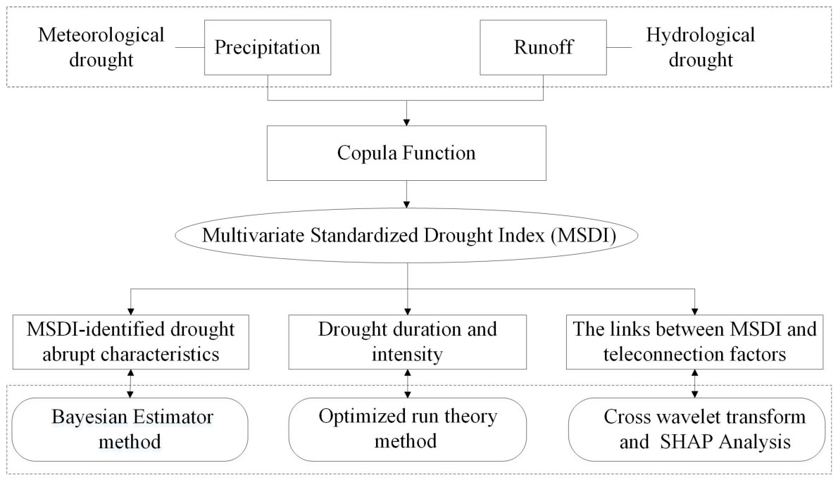
In this study, we developed a comprehensive analytical framework to construct a multivariate standardized drought index (MSDI) that integrates meteorological (precipitation) and hydrological (runoff) information. First, optimal marginal distributions and a Copula function were selected through goodness-of-fit tests to build the joint distribution of precipitation and runoff, from which the MSDI was derived. Based on the MSDI, the BEAST method was applied to detect abrupt changes in drought characteristics at the CTG hydrological station in the CSDIA. Optimized run theory was then employed to identify the duration and intensity of compound drought events. Finally, the possible driving forces of drought evolution were explored by linking the MSDI with large-scale teleconnection factors using cross-wavelet transform and SHAP analysis. The complete methodological workflow is illustrated in Figure 2.

2.7. Software and Programming Languages

All numerical calculations and statistical analyses were performed using Python 3.9 and MATLAB R2019b. Python was employed for fitting the optimal marginal distributions (Section 3.1.1) and for the SHAP contribution analysis (Section 3.4.2), utilizing the scipy (v1.13.1), numpy (v2.0.2), scikit-learn (v1.6.1), and shap libraries(v0.49.1). MATLAB was used for Copula fitting (Section 3.1.1), construction of the multivariate standardized drought index (MSDI) (Section 3.1.2), abrupt change detection using the BEAST toolbox (Section 3.2), joint return period analysis of drought duration and intensity (Section 3.3), and cross-wavelet analysis (Section 3.4.1), with the help of the Statistics and Machine Learning Toolbox (v11.6), the BEAST toolbox (v1.0), and the Wavelet toolbox (v5.3).

3. Results

3.1. Construction of the MSDI

3.1.1. Marginal Distributions and Copula Selection

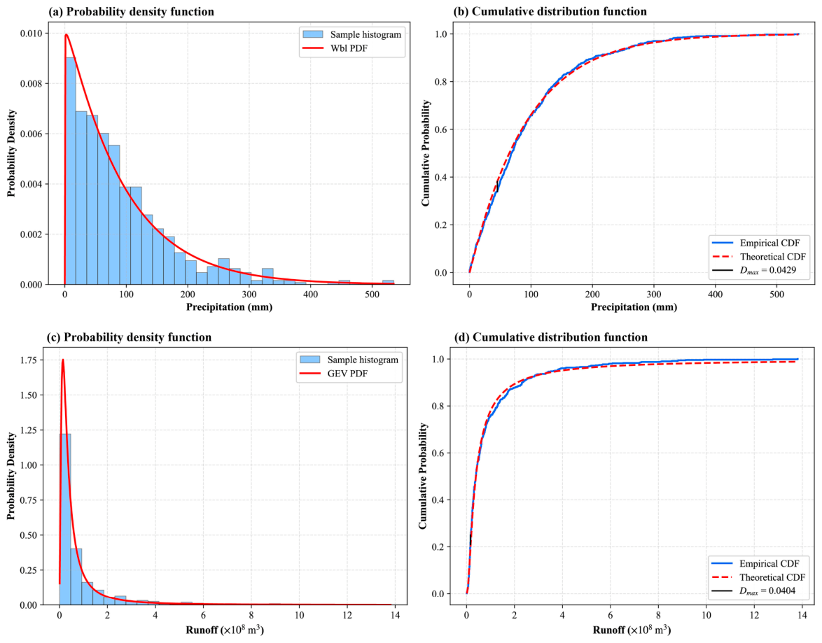
At a significance level of α = 0.05, six candidate distributions were evaluated for each variable using the K-S test. Three distributions passed the K-S test for precipitation (Wbl, GEV, and Log-L), and two passed for runoff (GEV and Log-L). Among the passing candidates, the optimal marginal distribution was selected as the one with the smallest A-D statistic, which is more sensitive to deviations in the tails of the distribution. This yielded Wbl (A-D = 1.385) for precipitation and GEV (A-D = 1.420) for runoff as the optimal marginal distributions (Table 2), both indicating no significant deviation from the theoretical distributions.
Figure 3 shows the fitted theoretical probability density functions (PDFs) and cumulative distribution function (CDF) against empirical frequencies. The precipitation PDF exhibits a unimodal right-skewed shape, peaking at approximately 50 mm and then declining slowly, reflecting the frequent occurrence of moderate rainfall events in the region. The runoff PDF shows a sharp peak at low flow values, followed by a rapid decay, indicating that low-flow conditions dominate the hydrological regime. The CDF for both variables align closely with empirical points, confirming that the selected distributions adequately capture the statistical characteristics. The excellent goodness of fit shown in Figure 3 is attributed to several factors. First, the fitting is based on monthly precipitation and runoff series from 1960 to 2018, comprising 708 data points, which provides a sufficiently large sample size for reliable distribution fitting. Second, monthly aggregated data are inherently smoother than daily data, as high-frequency noise has been filtered out. Third, both the Wbl (for precipitation) and GEV (for runoff) distributions are highly flexible and have been widely proven effective for modeling skewed hydrological variables over long time series. Fourth, the K-S test p-values (0.144 for precipitation and 0.192 for runoff) indicate no significant deviation between the theoretical and empirical distributions, statistically validating the fits. Therefore, the smooth and high-quality fits in Figure 3 are realistic and consistent with the statistical characteristics of the data.
Among the five Copula candidates, the Gumbel Copula consistently outperformed all others across multiple goodness-of-fit criteria (Table 3), yielding the highest NSE (0.9957) and log-likelihood (291.08), as well as the lowest RMSE (0.5271), AIC (−580.16), and BIC (−575.60). The margins over the second-best candidate (Frank Copula) are substantial, with a log-likelihood difference of 57.36 and a BIC difference of 114.72, leaving no ambiguity in the selection. Therefore, the Gumbel Copula was used to construct the joint distribution of precipitation and runoff.

3.1.2. Applicability of the MSDI

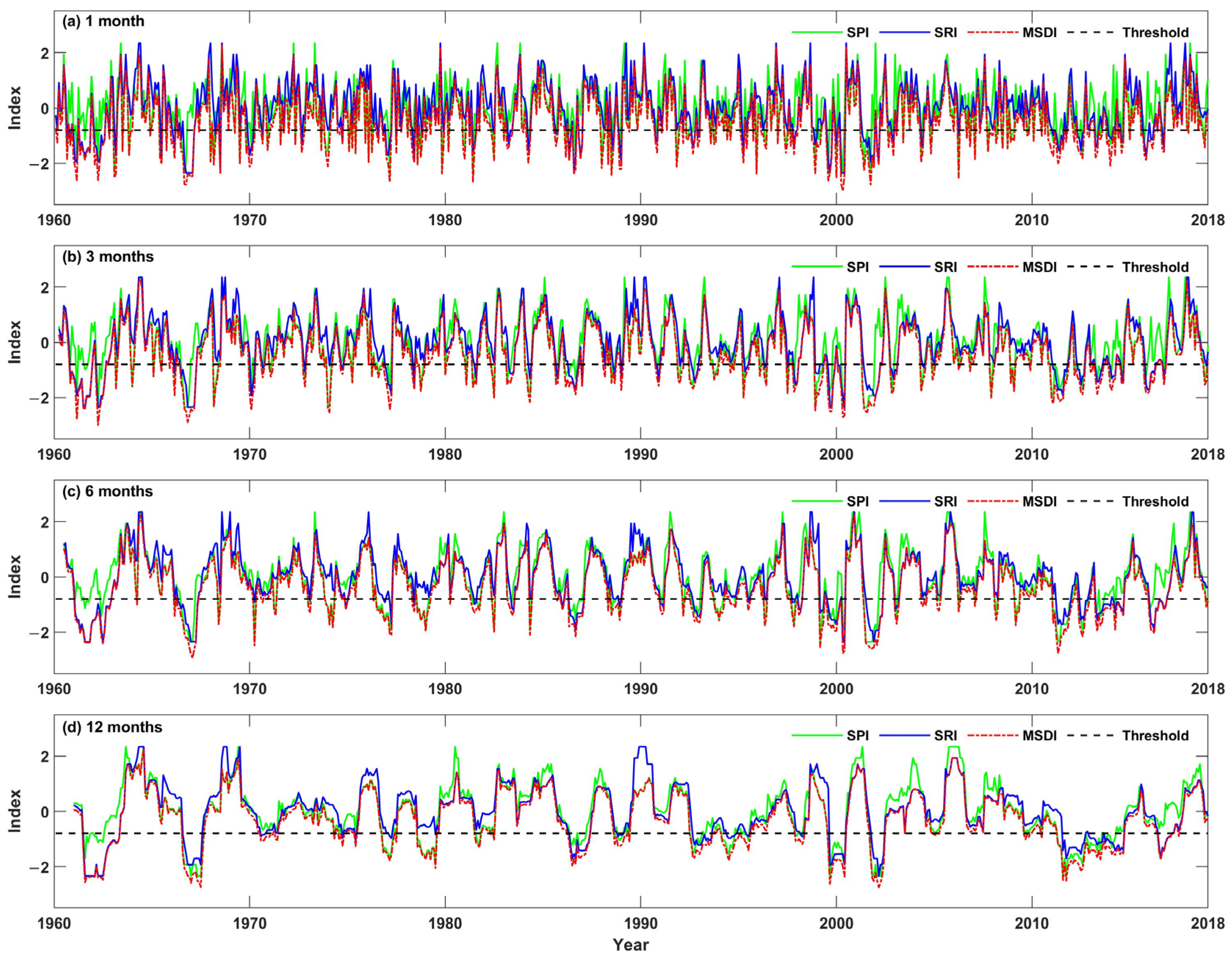
Figure 4 presents the monthly SPI, SRI, and MSDI at different time scales (1–24 months) from 1960 to 2018. The three indices show strong visual coherence, with peaks and troughs occurring simultaneously in most periods. Quantitative analysis reveals Pearson correlation coefficients of 0.76 between MSDI and SPI and 0.92 between MSDI and SRI, both exceeding 0.75 and significant at the 1% level (p < 0.01). These high correlations confirm that MSDI reliably captures the combined signal of meteorological and hydrological drought.
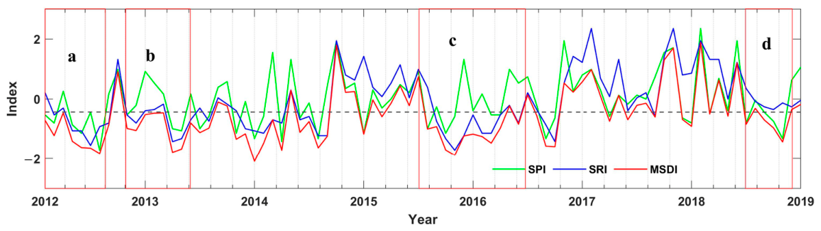
To provide a more intuitive comparison, the monthly SPI, SRI, and MSDI at the CTG station from 2012 to 2018 are extracted and shown in Figure 5, and the drought events identified by each index during four representative periods are summarized in Table 4. It is generally accepted that drought onset is usually triggered by reduced precipitation, so SPI is more sensitive to the beginning of drought. In contrast, due to the influence of runoff generation and concentration processes, hydrological drought responds to meteorological drought with a certain lag, making SRI more effective at reflecting the duration and termination of drought. As shown in Table 4, during Events a (2012) and b (2012–2013), MSDI detected drought onset in January 2012 and October 2012, respectively, which were 3 and 5 months earlier than the corresponding SPI onsets (April 2012 and March 2013), demonstrating MSDI’s superior sensitivity in capturing drought initiation through the integration of both meteorological and hydrological information. During Events c (2015–2016) and d (2018), MSDI captured drought termination in June 2016 and November 2018, respectively, which were 1 and 2 months later than the corresponding SRI terminations (May 2016 and September 2018), reflecting MSDI’s ability to track the prolonged impact of compound water deficits beyond the recovery of a single variable. These results indicate that MSDI combines the strengths of SPI and SRI and can sensitively and effectively capture the onset, duration, and termination of drought.
It should be noted that MSDI is not a simple linear average of SPI and SRI. Instead, it is derived from the joint cumulative probability P = C ( F prec ( x ) , F runoff ( y ) ) via a Copula function. When both precipitation and runoff are simultaneously dry, the joint probability P is generally less than or equal to each marginal probability (i.e., P m i n ( F prec , F runoff ) ). Consequently, the transformed MSDI becomes more negative (drier) than both SPI and SRI. This behavior reflects the aggravating effect of compound drought: the combined water deficit from both meteorological and hydrological sources is more severe than either individual drought. In periods where only one variable is dry (e.g., hydrological drought without meteorological drought, or vice versa), MSDI typically falls between SPI and SRI or close to the drier one. Thus, the observation in Figure 4 that MSDI is sometimes the lowest is fully consistent with its mathematical definition and is indeed a desirable property for capturing compound drought severity.
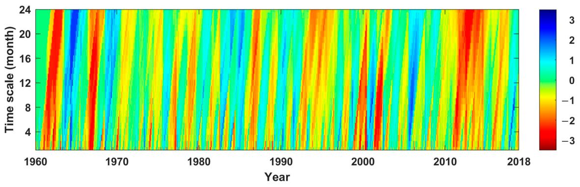
Figure 6 shows the time evolution of MSDI at scales of 1 to 24 months. Blue indicates wet conditions (less drought); red indicates dry conditions (more drought). Short time scales (1–3 months) exhibit high-frequency variability, reflecting rapid atmospheric fluctuations. As the time scale increases, the series becomes smoother, revealing longer-term trends. A notable shift occurs after the 1980s: from 1980 to 2018, red tones (drought) appear more frequently and with greater intensity compared to 1960–1980. The most severe drought periods identified by MSDI include 1960–1964, 1966–1967, 2001–2002, and 2010–2011, consistent with historical records of major droughts in the Huaihe River Basin.

3.2. Abrupt Change Detection of MSDI Using BEAST

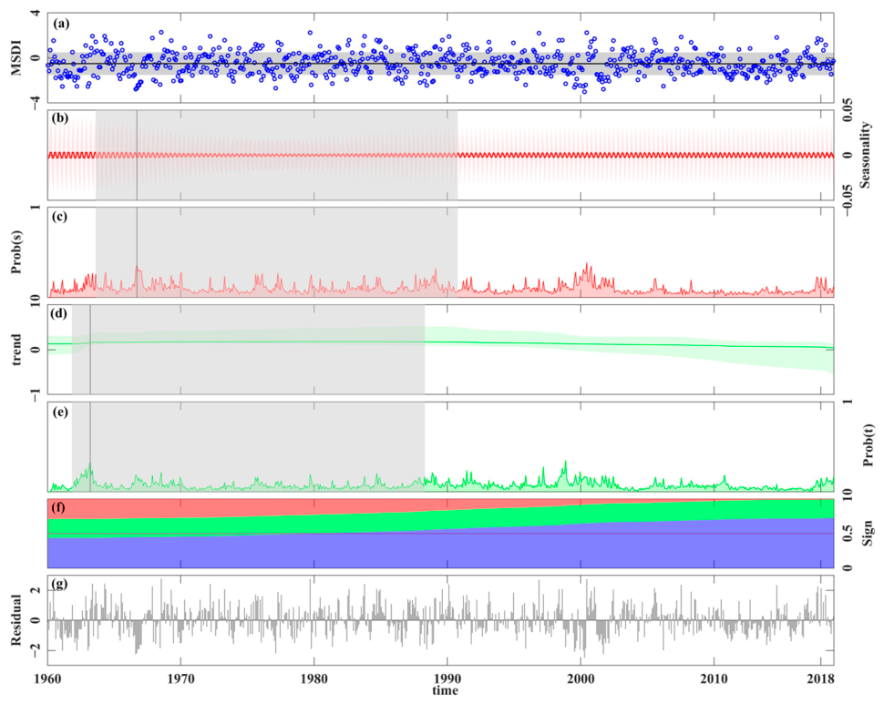
Figure 7 presents the BEAST decomposition of the MSDI series into trend, seasonal, and residual components, along with 75% confidence intervals. The seasonal component shows regular annual cycles, with positive anomalies (wetter) in winter–spring and negative anomalies (drier) in summer–autumn. The peak seasonal amplitude reaches approximately 0.6 in January–February. The Bayesian change-point analysis detects a seasonal change point in September 1966 with a probability of 56.70% (95% credible interval: August 1966–September 1990), suggesting a shift in the timing or amplitude of seasonal drought patterns around that period.
The trend component exhibits a two-phase evolution: from 1960 to 1990, the trend shows a slight positive slope (0.003 per year, p = 0.12, not significant), indicating a weak tendency toward wetter conditions. After 1990, the trend reverses to a negative slope (−0.007 per year, p = 0.04, significant), indicating a gradual intensification of drought. The change point in the trend occurs in March 1963 with 47.52% probability (95% CI: November 1961–April 1988). However, the overall magnitude of the trend change is modest (from +0.1 to −0.2 over 60 years), suggesting that while drought has become more frequent and severe, the signal is not extremely strong. The residual component is stationary with no obvious patterns, confirming that the decomposition has effectively captured the deterministic components.

3.3. Joint Distribution and Return Period of Drought Duration and Intensity

3.3.1. Sensitivity Analysis of Run Theory Thresholds

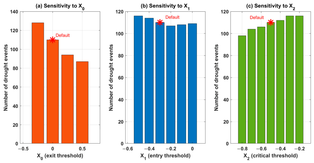
The three thresholds employed in the optimized run theory are selected based on established conventions in the standardized drought index literature. The exit threshold (X0 = 0) corresponds to the median of the standardized distribution; when the MSDI value recovers to zero or above, the drought episode is considered terminated, following the universal convention for standardized drought indices [46,47]. The entry threshold (X1 = −0.3) defines the boundary for identifying incipient dry months (MSDI ≤ −0.3), distinguishing normal variability from genuine drought onset. The critical threshold (X2 = −0.5) filters isolated dry months that do not meet moderate drought intensity, aligning with the classification standard of the U.S. National Drought Mitigation Center (NDMC), where SPI/MSDI values below −0.5 indicate moderate drought or worse. Using these thresholds, a total of 110 compound drought events were identified over the 1960–2018 study period.
As shown in Table 5 and Figure 8, the sensitivity of the three thresholds varied considerably. The critical threshold X2 was the most robust parameter: across all tested values (−0.80 to −0.20), the most severe event (1960.04–1961.06) was consistently identified with an invariant severity of 22.72 and a consistent longest drought duration of 15 months (core drought period), while event counts varied within a narrow range (99–115). The entry threshold X1 showed moderate sensitivity: event counts ranged from 106 to 115, and the longest event duration increased from 15 months (at X1 ≤ −0.3) to 18 months (at X1 ≥ −0.2), though the most severe event remained consistently identified at 1960.04–1961.06 across all tested values. The exit threshold X0 exhibited the greatest sensitivity, with event counts varying widely from 86 to 131 and the identified most severe event shifting from the 1960.04–1961.06 period (severity 22.72, 15 months) at X0 ≤ 0.00 to the 1960.04–1962.06 period (severity 37.01, 27 months) at X0 = 0.50. This heightened sensitivity arises because X0 directly governs the termination timing of drought episodes: a higher exit threshold delays drought recovery recognition, thereby merging consecutive dry spells into longer, more severe compound events. Detailed event counts and maximum durations for each tested value of all three thresholds are provided in Table 6. Figure 8 illustrates the sensitivity of identified drought event counts and key severity metrics to variations in each threshold, confirming that X2 produces the most stable results while X0 introduces the greatest variability. These results collectively confirm that the default threshold combination (X0 = 0, X1 = −0.3, and X2 = −0.5) provides a balanced and robust identification of compound drought events.

3.3.2. Identification and Statistical Characteristics of Drought Events

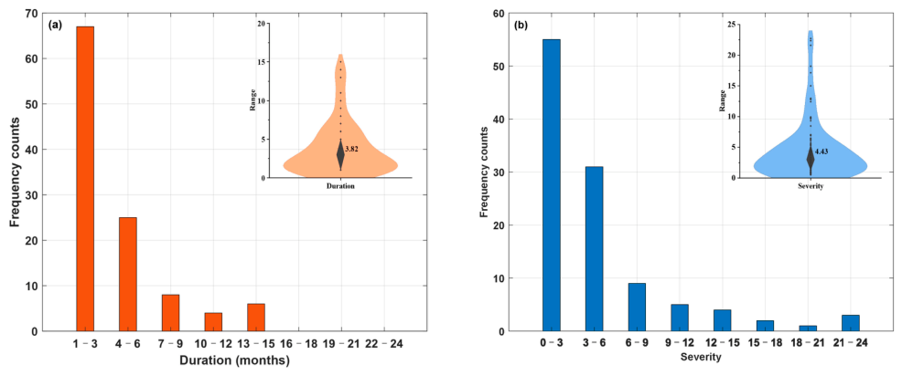
Using the optimized run theory, 110 compound drought events were identified from 1960 to 2018. Figure 9 shows the frequency distribution of event duration and intensity. The histogram for duration is strongly right-skewed: 67 events (61%) have a duration of 1–3 months, 25 events (23%) last 4–6 months, 8 events (7%) last 7–9 months, and only 10 events (9%) exceed 9 months. Similarly, the intensity distribution shows that 95 events (86%) have intensity values below 9, while only 15 events (14%) exceed 9. The average duration is 3.82 months, and the average intensity is 4.43. These statistics confirm that compound droughts in the CSDIA are predominantly short and mild, which is consistent with the general drought climatology of the Huaihe River Basin where droughts are often interrupted by frequent rainfall events.
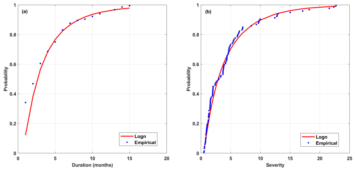
Figure 10 presents the optimal univariate marginal distributions for duration and intensity. The Logn distribution for duration (K-S statistic = 0.052, p = 0.64) provides an excellent fit, with the theoretical CDF closely tracking empirical points. For intensity, the Logn distribution (K-S statistic = 0.042, p = 0.72) is optimal, capturing the heavy-tailed nature of extreme intensities. The Pearson correlation between duration and intensity is 0.91 (p < 0.005), indicating a near-linear positive relationship: longer droughts tend to be more intense. This strong dependence justifies the use of a bivariate Copula model.
Among the five Copula candidates, the Clayton Copula consistently outperformed all others across multiple goodness-of-fit criteria (Table 6), yielding the highest NSE (0.9437), highest log-likelihood (101.27), and lowest AIC (−200.53) and BIC (−197.83). Although the Gaussian Copula achieved comparable NSE and RMSE values (0.9437 and 0.7056, respectively), the Clayton Copula was substantially superior in terms of log-likelihood and information-theoretic criteria, providing unambiguous support for its selection. Moreover, the Clayton Copula is particularly suitable for modeling lower-tail dependence, which effectively captures the predominant pattern in the data where both drought duration and intensity are simultaneously at their lower values—an observation consistent with the finding that 61% of compound drought events have durations of 1–3 months and 86% have intensity values below 9 (Figure 9).
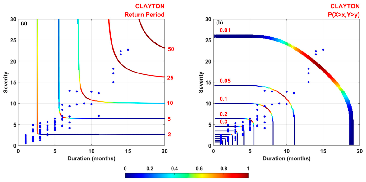
Figure 11 shows the joint return period isolines (in years) for combined events exceeding given duration and intensity thresholds. The red dots represent the 110 historical drought events. Most dots fall within the region of return periods less than 10 months, confirming that common droughts are frequent. As duration and intensity increase, the return period increases exponentially. For example, a drought with duration = 12 months and intensity = 15 has a return period of about 20 years. The most severe event identified in the entire record occurred from August 1960 to October 1961, with a duration of 15 months and an intensity of 22.72. This event lies very close to the 40-year return period isoline, with an estimated joint exceedance probability of approximately 0.025 (2.5%).

3.4. Driving Forces of Compound Drought

3.4.1. Cross-Wavelet Analysis

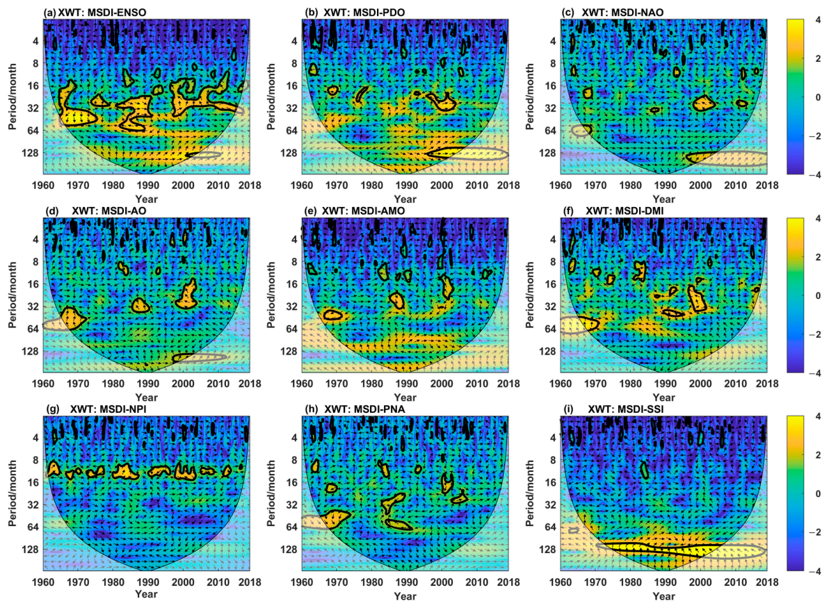
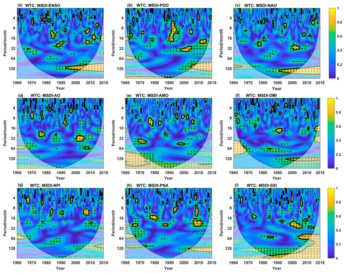
Figure 12 shows the cross-wavelet power spectra between monthly MSDI and the nine teleconnection factors. MSDI exhibits three significant resonance periods with ENSO: a positive correlation at 32–60 months (1966–1975), a positive correlation at 24–64 months (1986–1992), and a negative correlation at 15–35 months (1995–2010). MSDI also shows positive correlations with PDO and NAO at 25–32 months (1995–2005). With AO, there are three significant periods: a positive correlation at 32–64 months (1965–1972) and two negative correlations at 30–40 months (1985–1990) and 16–38 months (1995–2005). PNA shows a positive correlation at 48–64 months (1965–1975). Intermittent oscillations are observed for AMO and DMI (8–32 months), NPI (8–16 months), and PNA (16–64 months). SSI shows a significant negative correlation at 120–130 months (1972–2008). Overall, ENSO is the most influential driver, followed by SSI. In the low-energy region (Figure 13), MSDI exhibits intermittent 8–16 month oscillations with all factors, but no persistent significant coherence, indicating that deterministic forcing is weak at low power levels.
Previous studies have shown that ENSO events have a significant impact on drought and flood anomalies in the Yangtze-Huai River region, with different phases of ENSO corresponding to distinct spatial patterns of precipitation anomalies: the El Niño developing phase and the La Niña decaying phase are often associated with increased summer precipitation over the region, whereas the El Niño decaying phase and the La Niña developing phase correspond to decreased precipitation. Furthermore, ENSO often interacts synergistically with other climate factors such as DMI and NAO to influence drought evolution in the Huaihe River Basin.

3.4.2. SHAP Contribution Analysis

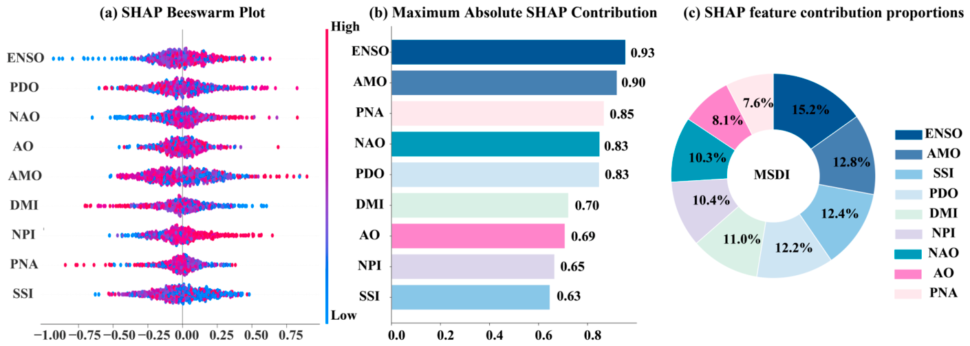
Figure 14 presents the explainability analysis results of the quantitative driving mechanisms of multi-scale climate factors on the Multi-Scale Drought Index (MSDI). Specifically, Figure 14a characterizes the directionality and dispersion features of each factor’s influence on drought, where positive SHAP values indicate an aggravating effect on drought severity, whereas negative values denote a mitigating effect. Figure 14b further quantifies the maximum absolute contribution intensity of each factor under extreme conditions, and Figure 14c reveals the overall feature contribution proportions of each factor across the full dataset.
Based on the comprehensive analysis of the three subfigures, ENSO exhibits a prominent dual-driven effect in the evolution of MSDI: its local extreme contribution value (0.93) and global feature contribution proportion (15.2%) are both the highest among all teleconnection factors, indicating that ENSO not only exerts a significant instantaneous triggering effect on regional extreme drought–flood abrupt events but also continuously modulates the overall drought evolution pattern over longer time scales. The driving modes of individual factors demonstrate a pronounced temporal differentiation between “high-frequency pulse type” and “low-frequency gradual type.” Specifically, PNA exhibits a typical short-term triggering characteristic, with a local extreme value of 0.85 but a global contribution of only 7.6%, suggesting that its influence is predominantly concentrated in the triggering phase of extreme events. In contrast, SSI displays an opposite pattern: although its local extreme value is relatively low (0.63), its global contribution proportion reaches 12.5%, reflecting the sustained and steady-state regulatory effect of long-period external forcings on regional hydrological cycles. AMO and PDO possess both strong extreme driving capabilities (with extreme values of 0.90 and 0.83, respectively) and robust global explanatory power (with contribution proportions of 12.8% and 12.2%, respectively), exerting substantial impacts on the drought system across multiple time scales. Further analysis reveals that ENSO not only directly drives the onset of extreme events through its own vigorous phase transitions but also maintains cross-scale synergistic regulatory relationships with low-frequency oscillations such as AMO and PDO, as well as external forcing signals like SSI, thereby playing a comprehensive regulatory role that spans both high-frequency and low-frequency processes within the regional multi-scale drought driving network. These explainable analysis results mutually corroborate the findings derived from cross-wavelet coherence analysis, further validating the robustness and reliability of the identified driving mechanisms.

4. Discussion

4.1. Advantages

4.1.1. Comparisons with Previous Studies in Other Regions Worldwide

The compound drought characteristics identified in the CSDIA are generally consistent with drought patterns reported in monsoon irrigation regions across China and other global catchments. Similarly to the Huaihe River Basin [48,49] and other East Asian monsoon basins [50], drought events in the CSDIA are dominated by short durations (average 3.82 months) and low-to-moderate intensities, with extreme droughts occurring at multidecadal to centennial return intervals [51]. This feature is also comparable to irrigation areas in the middle and lower Yangtze River Basin, where frequent intermittent rainfall interrupts drought development and restricts prolonged severe droughts [52].
Globally, droughts in Mediterranean agricultural regions and semi-humid subtropical irrigation basins also exhibit similar right-skewed distributions in drought duration and intensity, with most events concentrated in short-term and low-magnitude categories [53]. The dominant driving role of ENSO identified in this study further agrees with findings from many Asian, Australian, and American river basins, confirming that ENSO acts as a critical large-scale teleconnection modulating interannual drought variability across monsoon and subtropical climate zones [54,55]. The most severe drought event detected in the CSDIA (August 1960–October 1961, duration 15 months, intensity 22.72, return period approximately 40 years) is consistent with historical drought records in the Huaihe River Basin, which documented severe and prolonged drought conditions during this period [56].

4.1.2. Advantages of the Proposed Methodology over Conventional Approaches

The methodological framework adopted in this study shows clear improvements over traditional drought evaluation methods. First, conventional drought indices such as SPI and SRI only reflect meteorological or hydrological drought individually and cannot capture the interactive propagation between rainfall deficit and runoff reduction [57]. By constructing the Copula-based multivariate standardized drought index (MSDI), this study integrates precipitation and runoff, effectively characterizing compound drought processes and accurately capturing drought onset, development, and termination [58]. Correlation results (Pearson’s r > 0.75) further verify the reliability and superiority of MSDI over single indices [59].
Second, traditional composite drought indices mostly rely on linear weighting or dimension-reduction methods (e.g., principal component analysis and entropy weight method), which assume linear dependence and cannot describe the nonlinear correlation between hydrometeorological variables. In contrast, Copula functions flexibly fit different marginal distributions and depict complex nonlinear joint relationships, providing higher fitting accuracy and stronger applicability for drought index construction [60].
Third, the combination of BEAST abrupt change detection, cross-wavelet transform, and SHAP contribution analysis is superior to conventional trend tests and simple correlation analysis. BEAST can probabilistically detect trend and seasonal abrupt changes without deterministic threshold constraints; cross-wavelet transform reveals multi-scale time-frequency resonance between drought and climate factors [61,62]; SHAP further quantitatively ranks the marginal contribution of each teleconnection factor. This integrated framework provides more robust, comprehensive, and interpretable driving force quantification than traditional single-method analysis [63].

4.1.3. Implications for Sustainable Water Management

The findings of this study carry direct implications for the sustainable management of water resources in the CSDIA and comparable irrigation systems. The identification of 110 compound drought events over 59 years, with a notable intensification trend after 1990, signals an escalating threat to long-term water availability. The dominance of ENSO as a driving force suggests that seasonal climate forecasting—leveraging ENSO phase information—could be integrated into reservoir operation rules to enable anticipatory water allocation, thereby reducing vulnerability to compound drought. Furthermore, the approximately 40-year return period of the most severe drought event provides a quantitative basis for designing drought contingency plans and infrastructure resilience standards. These insights support the transition from reactive to proactive drought management, which is a cornerstone of sustainable water governance.

4.2. Limitations

Several limitations should be acknowledged. First, the BEAST algorithm’s change-point detection depends on prior settings; different configurations might lead to different locations or probabilities. Second, this study relies on a single hydrological station and five meteorological stations. Although the CSDIA terrain is relatively flat (40–140 m elevation) and we have validated the station-interpolated precipitation against TRMM satellite data, the limited station network may still introduce some uncertainty in capturing localized precipitation variability, particularly near the basin boundaries. Third, although the use of naturalized runoff (Section 2.2.1) effectively removes the long-term influence of upstream human interventions on the runoff series, the naturalization procedure relies on annual water balance ratios and does not explicitly resolve sub-annual processes such as reservoir filling rules, irrigation scheduling, or inter-basin water transfers. This limitation is unlikely to affect the identification of major drought events or their long-term trends, as confirmed by the high consistency between observed and naturalized series (Pearson’s r = 0.99). However, for monthly-scale drought propagation analysis—particularly the lag between meteorological and hydrological drought onset—the absence of dynamically modeled human interventions may introduce some uncertainty. Future studies should integrate real-time reservoir operation records, irrigation demand models, and physically based hydrological simulations to separately quantify the contributions of climate variability and human activities to compound drought evolution.

5. Conclusions

Based on the comprehensive construction of the multivariate drought index, identification of compound drought events, analysis of evolution characteristics, and investigation of driving mechanisms, the following main conclusions are drawn:
(1)
A multivariate standardized drought index (MSDI) was developed based on the Copula function, integrating precipitation and runoff. MSDI correlates strongly with SPI and SRI (r > 0.75, p < 0.01) and effectively captures the onset, duration, and termination of drought events.
(2)
From 1960 to 2018, 110 compound drought events were identified in the CSDIA, characterized predominantly by short duration (mean 3.82 months) and low intensity (mean 4.43). The most severe event (August 1960–October 1961) has a return period of approximately 40 years.
(3)
BEAST change-point detection revealed a slight drought alleviation trend before 1990 and a mild intensification after 1990. The seasonal component peaks in winter–spring, with a change point in September 1966 (probability 56.7%).
(4)
Cross-wavelet and SHAP analyses consistently identified ENSO as the dominant driver of compound drought in the area, followed by SSI and PDO. These results provide a scientific basis for drought monitoring and water resource management.
Overall, this study contributes to the sustainability science of water resources by providing a robust, multi-variable framework for compound drought assessment. The identified drought characteristics and dominant climate drivers offer actionable information for designing adaptive water allocation policies, improving irrigation scheduling, and enhancing drought preparedness in the CSDIA. The methodological framework is transferable to other monsoon-dependent irrigation systems worldwide, supporting the United Nations Sustainable Development Goal 6 (Clean Water and Sanitation) and Goal 13 (Climate Action) by strengthening the evidence base for sustainable water management under climate variability.

Author Contributions

J.T.: Conceptualization, Methodology, Software, Writing—original draft, Validation. Z.X.: Methodology, Software, Investigation, Data curation, Visualization, Validation. Y.T.: Formal analysis, Resources, Writing—review and editing, Validation. Q.T.: Supervision, Project administration, Funding acquisition, Writing—review and editing, Conceptualization. All authors have read and agreed to the published version of the manuscript.

Funding

This research was funded by the Key R&D Program of Henan Province (project number: 251111210700, “Research and Application of Key Technologies for the Whole-Process Fine Regulation of Water Resources in Irrigation Districts Based on Digital Twins”) and the Zhongyuan Science and Technology Innovation Leading Talent Program (project number: 254200510037, “Key Technologies for Joint Regulation of Multiple Valves in Long-distance Water Diversion Projects”.

Institutional Review Board Statement

Not applicable.

Informed Consent Statement

Not applicable.

Data Availability Statement

Data available on request due to restrictions as the project is still under implementation.

Conflicts of Interest

Authors Junyue Tian and Zheng Xu was employed by the company Henan Chushandian Reservoir Irrigation Project Co., Ltd. The remaining authors declare that the research was conducted in the absence of any commercial or financial relationships that could be construed as a potential conflict of interest.

References

  1. Zhao, R.; Wang, H.; Hu, S.; Zhan, C.; Guo, J. Joint probability of drought encounter among three major grain production zones of China under nonstationary climate. J. Hydrol. 2021, 603, 126995. [Google Scholar] [CrossRef]
  2. Bevacqua, E.; Zappa, G.; Lehner, F.; Zscheischler, J. Precipitation trends determine future occurrences of compound hot-dry events. Nat. Clim. Change 2022, 12, 350–355. [Google Scholar] [CrossRef]
  3. Masson-Delmotte, V.; Zhai, P.; Pirani, A.; Connors, S.L.; Péan, C.; Berger, S.; Caud, N.; Chen, Y.; Goldfarb, L.; Gomis, M.I.; et al. Climate change 2021: The physical science basis. In Contribution of Working Group I to the Sixth Assessment Report of the Intergovernmental Panel on Climate Change; Cambridge University Press: Cambridge, UK, 2021; Volume 2, p. 2391. [Google Scholar]
  4. Liu, M.; Shen, Y.; Qi, Y.; Wang, Y.; Geng, X. Changes in precipitation and drought extremes over the past half century in China. Atmosphere 2019, 10, 203. [Google Scholar] [CrossRef]
  5. Asadnabizadeh, M. Critical findings of the sixth assessment report (AR6) of working Group I of the intergovernmental panel on climate change (IPCC) for global climate change policymaking a summary for policymakers (SPM) analysis. Int. J. Clim. Change Strateg. Manag. 2023, 15, 652–670. [Google Scholar]
  6. Yue, Y.; Liu, H.; Mu, X.; Qin, M.; Wang, T.; Wang, Q.; Yan, Y. Spatial and temporal characteristics of drought and its correlation with climate indices in Northeast China. PLoS ONE 2021, 16, e0259774. [Google Scholar] [CrossRef] [PubMed]
  7. Hao, Z.; Singh, V.P. Drought characterization from a multivariate perspective: A review. J. Hydrol. 2015, 527, 668–678. [Google Scholar] [CrossRef]
  8. McKee, T.B.; Doesken, N.J.; Kleist, J. The relationship of drought frequency and duration to time scales. In Proceedings of the 8th Conference on Applied Climatology, Anaheim, CA, USA, 17–22 January 1993; Volume 17, pp. 179–183. [Google Scholar]
  9. Shukla, S.; Wood, A.W. Use of a standardized runoff index for characterizing hydrologic drought. Geophys. Res. Lett. 2008, 35, L02405. [Google Scholar] [CrossRef]
  10. Palmer, W.C. Meteorological Drought; US Department of Commerce, Weather Bureau: Silver Spring, MD, USA, 1965. [Google Scholar]
  11. Rajsekhar, D.; Singh, V.P.; Mishra, A.K. Integrated drought causality, hazard, and vulnerability assessment for future socioeconomic scenarios: An information theory perspective. J. Geophys. Res. Atmos. 2015, 120, 6346–6378. [Google Scholar] [CrossRef]
  12. Hao, Z.; AghaKouchak, A.; Nakhjiri, N.; Farahmand, A. Global integrated drought monitoring and prediction system. Sci. Data 2014, 1, 140001. [Google Scholar] [CrossRef] [PubMed]
  13. Wang, J.; Wang, W.; Cheng, H.; Wang, H.; Zhu, Y. Propagation from meteorological to hydrological drought and its influencing factors in the Huaihe River Basin. Water 2021, 13, 1985. [Google Scholar] [CrossRef]
  14. Sklar, M. Fonctions de répartition à n dimensions et leurs marges. Ann. l’ISUP 1959, 8, 229–231. [Google Scholar]
  15. Shiau, J.T.; Modarres, R. Copula-based drought severity-duration-frequency analysis in Iran. Meteorol. Appl. A J. Forecast. Pract. Appl. Train. Tech. Model. 2009, 16, 481–489. [Google Scholar] [CrossRef]
  16. Li, Z.; Shao, Q.; Tian, Q.; Zhang, L. Copula-based drought severity-area-frequency curve and its uncertainty, a case study of Heihe River basin, China. Hydrol. Res. 2020, 51, 867–881. [Google Scholar] [CrossRef]
  17. Kao, S.C.; Govindaraju, R.S. A copula-based joint deficit index for droughts. J. Hydrol. 2010, 380, 121–134. [Google Scholar] [CrossRef]
  18. Hao, Z.; AghaKouchak, A. Multivariate standardized drought index: A parametric multi-index model. Adv. Water Resour. 2013, 57, 12–18. [Google Scholar] [CrossRef]
  19. Zhao, Q.; Zhang, X.; Li, C.; Xu, Y.; Fei, J. Compound ecological drought assessment of China using a Copula-based drought index. Ecol. Indic. 2024, 164, 112141. [Google Scholar] [CrossRef]
  20. Yu, X.; Zeng, X.; Brocca, L.; Gui, D.; Wang, D.; Wu, J. A copula-based composite drought index for enhanced drought monitoring and analysis. J. Geophys. Res. Atmos. 2025, 130, E2024JD041867. [Google Scholar] [CrossRef]
  21. Terzi, T.B.; Önöz, B. Advanced drought analysis using a novel copula-based multivariate index: A case study of the Ceyhan River Basin. Sustain. Water Resour. Manag. 2025, 11, 11. [Google Scholar] [CrossRef]
  22. Wang, F.; Wang, Z.; Yang, H.; Di, D.; Zhao, Y.; Liang, Q. A new copula-based standardized precipitation evapotranspiration streamflow index for drought monitoring. J. Hydrol. 2020, 585, 124793. [Google Scholar] [CrossRef]
  23. Das, S.; Das, J.; Umamahesh, N.V. Copula-based drought risk analysis on rainfed agriculture under stationary and non-stationary settings. Hydrol. Sci. J. 2022, 67, 1683–1701. [Google Scholar] [CrossRef]
  24. Qi, J.; Ma, D.; Chen, Z.; Tian, Q.; Tian, Y.; He, Z.; Ma, Q.; Ma, Y.; Guo, L. Runoff evolution characteristics and predictive analysis of Chushandian reservoir. Water 2025, 17, 2015. [Google Scholar] [CrossRef]
  25. Guo, X.; Cao, L.; Fang, Y.; Xu, J.; Li, C.; Ji, H. Integrating the AE-AM model and the SMI-P framework for water environmental security assessment: A case study of the Chushandian Reservoir basin. Ecol. Indic. 2025, 179, 114275. [Google Scholar] [CrossRef]
  26. Gan, R.; Li, D.; Chen, C.; Yang, F.; Ma, X. Impacts of climate change on extreme precipitation in the upstream of Chushandian Reservoir, China. Hydrol. Res. 2022, 53, 504–518. [Google Scholar] [CrossRef]
  27. Fang, Y.; Cao, L.; Guo, X.; Liang, T.; Wang, J.; Wang, N.; Chao, Y. Spatio-temporal heterogeneity of the ecological environment and its response to land use change in the Chushandian Reservoir Basin. Sustainability 2024, 16, 1385. [Google Scholar] [CrossRef]
  28. Ogunrinde, A.T.; Adigun, P.; Xian, X.; Yu, H.; Koji, D.; Adebiyi, A.; Sabo, A.A. Multi-scale drought variability over West Africa and the associated large-scale circulation patterns. Geomat. Nat. Hazards Risk 2024, 15, 2409199. [Google Scholar] [CrossRef]
  29. Liu, W.; Zhu, S.; Huang, Y.; Wan, Y.; Wu, B.; Liu, L. Spatiotemporal variations of drought and their teleconnections with large-scale climate indices over the Poyang Lake Basin, China. Sustainability 2020, 12, 3526. [Google Scholar] [CrossRef]
  30. Xiao, L.; Chen, X.; Zhang, R.; Zhang, Z. Spatiotemporal evolution of droughts and their teleconnections with large-scale climate indices over Guizhou province in southwest China. Water 2019, 11, 2104. [Google Scholar] [CrossRef]
  31. Varol, T.; Atesoglu, A.; Ozel, H.B.; Cetin, M. Copula-based multivariate standardized drought index (MSDI) and length, severity, and frequency of hydrological drought in the Upper Sakarya Basin, Turkey. Nat. Hazards 2023, 116, 3669–3683. [Google Scholar] [CrossRef]
  32. Zavareh, M.M.; Mahjouri, N.; Rahimzadegan, M.; Rahimpour, M. A drought index based on groundwater quantity and quality: Application of multivariate copula analysis. J. Clean. Prod. 2023, 417, 137959. [Google Scholar] [CrossRef]
  33. Li, C.; Singh, V.P.; Mishra, A.K. A bivariate mixed distribution with a heavy-tailed component and its application to single-site daily rainfall simulation. Water Resour. Res. 2013, 49, 767–789. [Google Scholar] [CrossRef]
  34. Wen, Y.; Yang, A.; Kong, X.; Su, Y. A Bayesian-model-averaging copula method for bivariate hydrologic correlation analysis. Front. Environ. Sci. 2022, 9, 744462. [Google Scholar] [CrossRef]
  35. Naderi, K.; Moghaddasi, M.; Shokri, A. Drought occurrence probability analysis using multivariate standardized drought index and copula function under climate change. Water Resour. Manag. 2022, 36, 2865–2888. [Google Scholar] [CrossRef]
  36. Jamali, S.; Jönsson, P.; Eklundh, L.; Ardö, J.; Seaquist, J. Detecting changes in vegetation trends using time series segmentation. Remote Sens. Environ. 2015, 156, 182–195. [Google Scholar] [CrossRef]
  37. Dan’azumi, S.; Mamudu, L.; Aldrees, A. Climate change detection and attribution: Bayesian estimation of abrupt change, seasonality and trend model, and Mann-Kendall trend test approaches. J. Water Clim. Change 2025, 16, 1895–1911. [Google Scholar] [CrossRef]
  38. Abubakar, M.L.; Tanko, A.S.; Richifa, K.I.; Ahmed, M.S.; Abdussalam, A.F.; Mohammed, S. Analysis of trends and abrupt changes in streamflow via innovative polygon trend analysis and BEAST changepoint detection. World Water Policy 2025, 11, 820–835. [Google Scholar] [CrossRef]
  39. Palagiri, H.; Pal, M. Agricultural drought risk assessment in Southern Plateau and Hills using multi threshold run theory. Results Eng. 2024, 22, 102022. [Google Scholar] [CrossRef]
  40. Ma, Q.; Li, Y.; Liu, F.; Feng, H.; Biswas, A.; Zhang, Q. SPEI and multi-threshold run theory based drought analysis using multi-source products in China. J. Hydrol. 2023, 616, 128737. [Google Scholar] [CrossRef]
  41. Wang, J.; Li, J. Multi-threshold structural equation model. J. Bus. Amp Econ. Stat. 2023, 41, 377–387. [Google Scholar]
  42. Grinsted, A.; Moore, J.C.; Jevrejeva, S. Application of the cross wavelet transform and wavelet coherence to geophysical time series. Nonlinear Process. Geophys. 2004, 11, 561–566. [Google Scholar] [CrossRef]
  43. Souza, E.M.; Félix, V.B. Wavelet cross-correlation in bivariate time-series analysis. TEMA 2018, 19, 391–403. [Google Scholar] [CrossRef]
  44. Štrumbelj, E.; Kononenko, I. Explaining prediction models and individual predictions with feature contributions. Knowl. Inf. Syst. 2014, 41, 647–665. [Google Scholar]
  45. Slack, D.; Hilgard, S.; Jia, E.; Singh, S.; Lakkaraju, H. Fooling lime and shap: Adversarial attacks on post hoc explanation methods. In Proceedings of the AAAI/ACM Conference on AI, Ethics, and Society, New York City, New York, USA, 7–8 February 2020; pp. 180–186. [Google Scholar]
  46. Mukhawana, M.B.; Kanyerere, T.; Kahler, D.; Masilela, N.S.; Lalumbe, L.; Umunezero, A.A. Hydrological drought assessment using the standardized groundwater index and the standardized precipitation index in the Berg River Catchment, South Africa. J. Hydrol. Reg. Stud. 2024, 53, 101779. [Google Scholar] [CrossRef]
  47. Svoboda, M.; Hayes, M.; Wood, D. Standardized Precipitation Index: User Guide; World Meteorological Organization: Geneva, Switzerland, 2012. [Google Scholar]
  48. Yuqian, H.U.; Lei, H.U.; Peng, S.U.N.; Qingzhi, W.E.N.; Anlan, F.E.N.G.; Wei, L.I.U. Spatio-temporal evolution of drought events in Huaihe River Basin: A non-stationary standardized precipitation evapotranspiration index study. J. Beijing Norm. Univ. 2022, 58, 116–124. [Google Scholar]
  49. Yao, H.; Li, Q.; Zhao, L.; Wu, X.; Shen, X.; Duan, C.; Li, C. Evolution characteristics of compound drought and heat events during the warm season in the Huaihe River Basin and their relationship with climate and vegetation. Acta Ecol. Sin. 2024, 44, 5596–5608. [Google Scholar] [CrossRef]
  50. Huang, L.; Du, H.; Dang, Y.; He, H.S.; Wang, L.; Na, R.; Li, N.; Wu, Z. Observed and projected changes in wet and dry spells for the major river basins in East Asia. Int. J. Climatol. 2023, 43, 5369–5386. [Google Scholar] [CrossRef]
  51. Muthuvel, D.K.; Qin, X.S. Probabilistic analysis of future drought propagation, persistence, and spatial concurrence in monsoon-dominant Asian regions under climate change. Hydrol. Earth Syst. Sci. 2025, 29, 3203–3225. [Google Scholar] [CrossRef]
  52. Yang, P.; Zhang, S.; Xia, J.; Zhan, C.; Cai, W. Analysis of drought and flood alternation and its driving factors in the Yangtze River Basin under climate change. Atmos. Res. 2022, 270, 106087. [Google Scholar] [CrossRef]
  53. Raut, A.; Ganguli, P. Onset seasonality controls compound streamflow drought risk at a global scale. npj Nat. Hazards 2026. [Google Scholar] [CrossRef]
  54. Bhatia, U.; Poonia, H.; Tantary, D.M.; Mishra, V.; Kumar, R. Regional responses to oceanic variability constrain global drought synchrony. Commun. Earth Environ. 2026, 7, 86. [Google Scholar] [CrossRef]
  55. Lieber, R.; Brown, J.; King, A.; Freund, M. Historical and future asymmetry of ENSO teleconnections with extremes. J. Clim. 2024, 37, 5909–5924. [Google Scholar] [CrossRef]
  56. Li, X.; Fang, G.; Wen, X.; Xu, M.; Zhang, Y. Characteristics analysis of drought at multiple spatiotemporal scale and assessment of CMIP6 performance over the Huaihe River Basin. J. Hydrol. Reg. Stud. 2022, 41, 101103. [Google Scholar] [CrossRef]
  57. Kanthavel, P.; Saxena, C.K.; Singh, R.K. Integrated drought index based on vine copula modelling. Int. J. Clim. 2022, 42, 9510–9529. [Google Scholar] [CrossRef]
  58. Terzi, T.B.; Üçüncü, O. A novel statistical framework for constructing multivariate standardized drought indices. Theor. Appl. Climatol. 2025, 156, 539. [Google Scholar] [CrossRef]
  59. Terzi, T.B.; Önöz, B. Drought analysis based on nonparametric multivariate standardized drought index in the Seyhan River Basin. Nat. Hazards 2025, 121, 11051–11078. [Google Scholar] [CrossRef]
  60. Zhang, G.; Zhang, S.; Wang, H.; Gan, T.Y.; Su, X.; Wu, H.; Shi, L.; Xu, P.; Fu, X. Evaluating vegetation vulnerability under compound dry and hot conditions using vine copula across global lands. J. Hydrol. 2024, 631, 130775. [Google Scholar] [CrossRef]
  61. Di Nunno, F.; Granata, F. Analysis of trends and abrupt changes in groundwater and meteorological droughts in the United Kingdom. J. Hydrol. 2024, 637, 131430. [Google Scholar] [CrossRef]
  62. Di Nunno, F.; de Marinis, G.; Granata, F. Analysis of SPI index trend variations in the United Kingdom-A cluster-based and bayesian ensemble algorithms approach. J. Hydrol. Reg. Stud. 2024, 52, 101717. [Google Scholar] [CrossRef]
  63. Fang, G.; Li, X.; Xu, M.; Wen, X.; Huang, X. Spatiotemporal variability of drought and its multi-scale linkages with climate indices in the huaihe river basin, central china and east China. Atmosphere 2021, 12, 1446. [Google Scholar] [CrossRef]
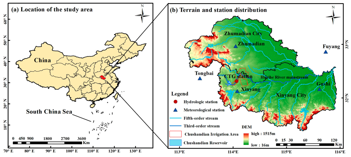
Figure 1. Location map of the CSDIA.
Sustainability 18 07598 g001
Figure 2. Flowchart of the research methodology.
Sustainability 18 07598 g002
Figure 3. Fitting of optimal marginal distributions for precipitation and runoff.
Sustainability 18 07598 g003
Figure 4. Comparison of SPI, SRI, and MSDI at monthly scale from 1960 to 2018. Pearson correlation coefficients between MSDI and SPI (0.76) and between MSDI and SRI (0.92) are both significant at p < 0.01.
Sustainability 18 07598 g004
Figure 5. Comparison of SPI, SRI, and MSDI during selected periods.
Sustainability 18 07598 g005
Figure 6. Multi-scale (1–24 months) time evolution of MSDI.
Sustainability 18 07598 g006
Figure 7. BEAST-based decomposition of MSDI (1960–2018): (a) Original MSDI observations; (b) seasonal component, with the red line representing the seasonal term; (c) posterior probability of a change in the trend component; (d) trend component, with the line representing the trend term; (e) posterior probability of a trend change; (f) posterior probabilities of the signs of the trend components; and (g) residual component. The gray-shaded areas in the relevant subfigures indicate the confidence intervals.
Sustainability 18 07598 g007
Figure 8. Sensitivity analysis of optimized run theory thresholds showing the number of identified compound drought events under varying (a) exit thresholds X0 (with X1 = −0.3 and X2 = −0.5 fixed), (b) entry thresholds X1 (with X0 = 0 and X2 = −0.5 fixed), and (c) critical thresholds X2 (with X0 = 0 and X1 = −0.3 fixed). Red asterisks indicate default threshold values.
Sustainability 18 07598 g008
Figure 9. Frequency distribution of duration and intensity of compound drought events: (a) Frequency distribution of event duration, with the inset violin plot showing the overall distribution and a central value of 3.82; (b) frequency distribution of event intensity, with the inset violin plot showing the overall distribution and a central value of 4.43.
Sustainability 18 07598 g009
Figure 10. Optimal univariate distribution fitting for drought duration and intensity.(a) Empirical and fitted cumulative distribution functions of drought duration; (b) empirical and fitted cumulative distribution functions of drought severity.
Sustainability 18 07598 g010
Figure 11. Joint return period of drought duration and intensity based on the Clayton Copula. Colors indicate joint density (blue = low, red = high). (a) Joint return-period contours (2–50 years); (b) joint exceedance-probability contours (0.01–0.30). Blue dots indicate observed drought events, and colors represent joint density from low (blue) to high (red).
Sustainability 18 07598 g011
Figure 12. Cross-wavelet transform between monthly MSDI and teleconnection factors in the high-energy region. Thick contours indicate regions significant at the 95% confidence level, and arrows indicate phase relationships: rightward arrows represent positive correlation, whereas leftward arrows represent negative correlation.
Sustainability 18 07598 g012
Figure 13. Wavelet coherence between MSDI and teleconnection factors in the low-energy region. Thick contours indicate regions significant at the 95% confidence level, while arrows indicate phase relationships: rightward arrows represent positive correlation, whereas leftward arrows represent negative correlation.
Sustainability 18 07598 g013
Figure 14. SHAP feature importance evaluation of the impacts of climate factors on MSDI. (a) Beeswarm plot of local feature contributions; (b) maximum absolute SHAP contributions; (c) total feature contribution percentage.
Sustainability 18 07598 g014
Table 1. Drought classification based on MSDI.
Drought ClassificationMSDI Value
ExtremeMSDI ≤ −2.0
Severe−2.0 < MSDI ≤ −1.5
Moderate−1.5 < MSDI ≤ −1.0
Abnormally−1.0 < MSDI ≤ −0.5
No droughtMSDI > −0.5
Table 2. Optimal marginal distributions for precipitation and runoff at CTG station.
VariableOptimal DistributionDistributed Parameter
(Shape, Scale, Location)
A-D StatisticK-S StatisticK-S p-Value
PrecipitationWbl α = 1.02 , γ = 0 , β = 92.47 1.3850.0430.144
P-III α = 2.01 , γ = 90.87 , β = 91.37 2.8380.0550.027
GEV α = 0.35 , γ = 46.99 , β = 45.32 2.7710.0420.167
Log-L α = 1.84 , γ = 6.76 , β = 70.77 3.7340.0470.087
Logn α = 1.50 , γ = 0 , β = 51.05 23.7970.1290.000
GP α = 4.43 , γ = 0 , β = 2.27 193.980.4030.000
RunoffGEV α = 0.84 , γ = 0.27 , β = 0.28 1.4200.0400.192
Log-L α = 1.41 , γ = 0 , β = 0.41 2.9300.0470.084
Logn α = 1.20 , γ = 0 , β = 0.44 3.2830.0580.015
GP α = 0.46 , γ = 0.01 , β = 0.52 6.8940.0860.000
Wbl α = 0.81 , γ = 0 , β = 0.81 15.9770.1010.000
P-III α = 2.04 , γ = 0.71 , β = 0.72 18.6800.0910.000
Note: Bold values indicate the optimal distribution (best-fitting result).
Table 3. Goodness of fit of Copula functions for precipitation runoff joint distribution.
CopulaNSERMSELog-LikelihoodAICBICθ
Gaussian0.99350.6447220.48−438.09−433.530.680
T0.98340.9915246.34−488.67−479.554.425
Clayton0.98480.986997.69−193.38−188.810.881
Frank0.99370.6368233.72−465.44−460.885.991
Gumbel0.99570.5271291.08−580.16−575.602.103
Note: Bold values indicate the optimal Copula function (best-fitting result).
Table 4. Comparison of drought events identified by SPI, SRI, and MSDI during the four representative periods shown in Figure 5.
Drought EventsIndicatorDrought OnsetDrought TerminationDuration (Months)
Event a (2012)MSDIJanuary 2012August 20128
SPIApril 2012July 20124
SRIFebruary 2012August 20127
Event b (2012–2013)MSDIOctober 2012July 201310
SPIMarch 2013April 20132
SRIOctober 2012July 201310
Event c (2015–2016)MSDIJuly 2015June 201612
SPIJuly 2015October 20154
SRIAugust 2015May 201610
Event d (2018)MSDIJune 2018November 20186
SPIJune 2018October 20185
SRISeptember 2018September 20181
Table 5. Sensitivity analysis of optimized run theory thresholds for compound drought identification.
ParameterRange TestedDefaultEvent Count RangeLongest Event Duration
X0−0.25 to 0.50086–13115–27 months
X1−0.50 to 0.00−0.3106–11515–18 months
X2−0.80 to −0.20−0.599–11515 months (all values)
Table 6. Goodness of fit of Copula functions for drought duration intensity joint distribution.
CopulaNSERMSELog-LikelihoodAICBICθ
Gaussian0.94340.705688.223−174.45−171.750.9117
T0.93160.765489.055−174.11−168.711.1268
Clayton0.94370.7037101.270200.53−197.832.6631
Frank0.94260.710987.151−172.30−169.6012.1022
Gumbel0.94330.706849.977−97.95−95.253.5721
Note: Bold values indicate the optimal Copula function (best-fitting result).
Disclaimer/Publisher’s Note: The statements, opinions and data contained in all publications are solely those of the individual author(s) and contributor(s) and not of MDPI and/or the editor(s). MDPI and/or the editor(s) disclaim responsibility for any injury to people or property resulting from any ideas, methods, instructions or products referred to in the content.