Climate-Adaptive Passive Solar Shading Optimization for Building Retrofits and New Construction in Hot Low-Latitude and Cold High-Latitude Regions

Abstract

Passive solar shading must balance energy saving, daylight availability, glare control, and thermal comfort under contrasting climates. This study develops and validates a lightweight, interpretable light-thermal-energy coupling framework for early-stage shading optimization in building retrofits and new construction. It addresses two questions: how shading geometry, envelope performance, and thermal inertia should adapt to hot low-latitude and cold high-latitude regions, and how their coupled performance can be quantified. The framework combines solar geometry, the Perez radiation model, surface irradiance calculation, indoor ray tracing/voxel illuminance simulation, daylight glare probability (DGP) assessment, and a 6R3C (6-Resistance, 3-Capacitance) transient thermal network. A full-factorial matrix of 120 design combinations was evaluated using shading scale, glazing performance, envelope thermal resistance, and thermal mass as variables, with energy use, thermal response, daylight availability, and DGP as objectives. Results show climate-dependent thermal inertia: it stabilizes indoor temperature in cold regions but increases heat accumulation in hot regions. The optimal schemes satisfy visual comfort (DGP < 0.40) and achieve energy savings up to 44.2% for retrofits and 50.0% for new buildings in hot regions, and 14.6% in cold regions. The framework provides transparent decision support for climate-adaptive, low-carbon building design and complements EnergyPlus, TRNSYS, and Radiance. By supporting energy-efficient retrofits and climate-responsive new construction, the proposed approach contributes to sustainability by reducing dependence on mechanical heating and cooling, improving operational resource efficiency, and maintaining indoor thermal and visual comfort.

1. Introduction

Building operation is a major source of energy use and carbon emissions, making the improvement of building energy performance a key pathway toward sustainable development and carbon neutrality. Among various passive design strategies, climate-adaptive passive envelope solutions are widely recognized as cost-effective approaches because they reduce operational energy demand, maintain indoor environmental quality, and enhance long-term building sustainability without increasing mechanical energy consumption. 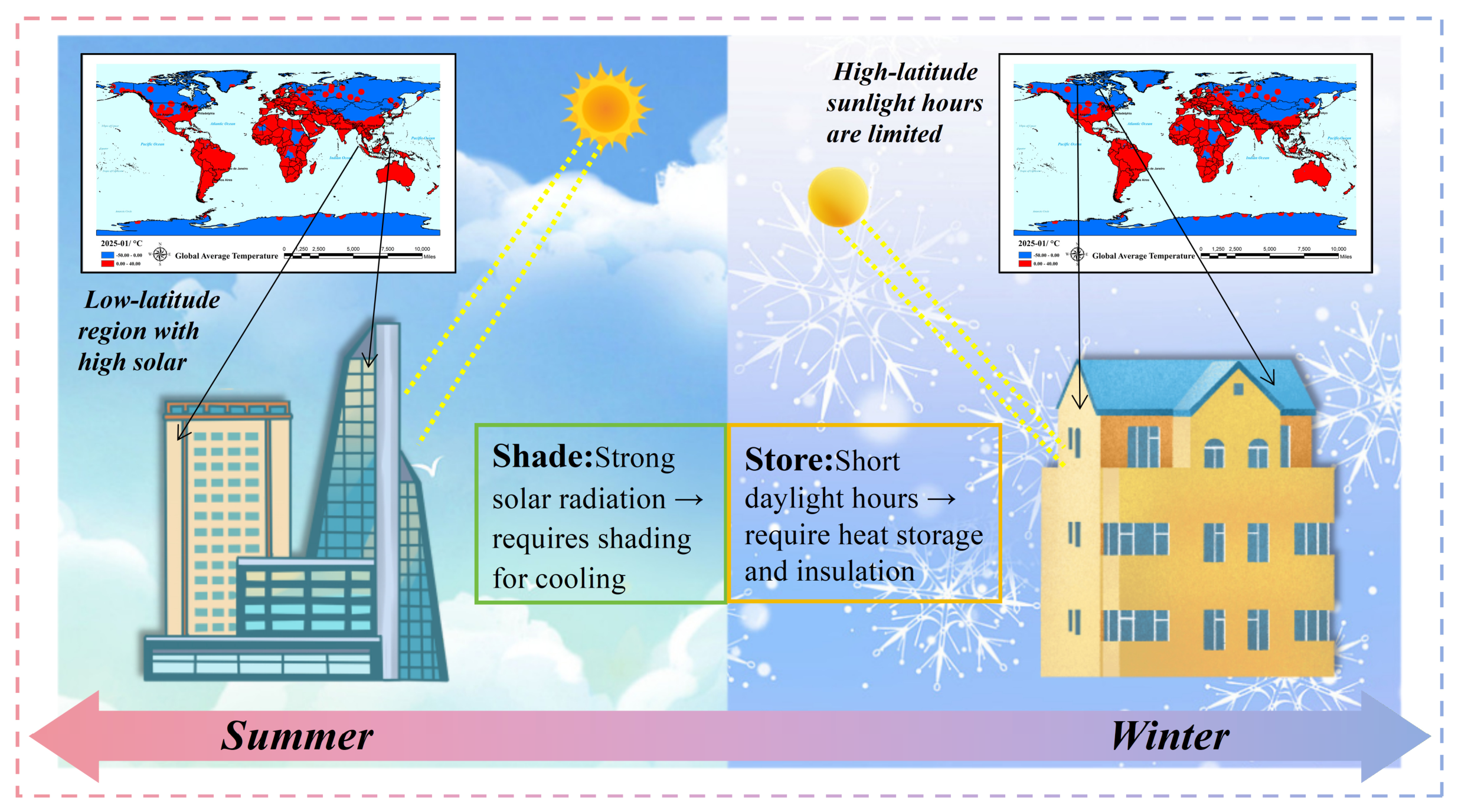The building envelope is the interface where solar heat gain, daylighting, glare risk, and heating/cooling loads interact most directly [1,2,3,4,5]. In hot, low-latitude regions, high solar elevation angles and sustained radiation increase cooling demand and overheating risk; in cold, high-latitude regions, low solar altitude, oblique radiation, and long heating seasons require a balance between winter solar gain, summer overheating prevention, and visual comfort. As illustrated in Figure 1, these contrasting solar-geometry and radiation conditions make passive shading a climate-specific design problem involving latitude, climate, orientation, window-to-wall ratio, envelope performance, and thermal inertia [6,7,8]. Consequently, optimizing passive solar shading is not only an effective energy-saving approach but also an important sustainable building strategy that supports low-carbon operation, climate adaptation, and occupant well-being.

Passive solar shading regulates direct, diffuse, and reflected solar radiation entering buildings, thereby reducing cooling loads, improving daylight uniformity, and limiting glare without additional active energy use [9,10,11,12,13,14]. It is increasingly regarded as a fundamental sustainable building technology that simultaneously improves energy efficiency, indoor environmental quality, and long-term building resilience under different climatic conditions. Recent studies have expanded from fixed overhangs and fins to louvers, grilles, egg-crate systems, vegetated and photovoltaic-integrated shading, smart glazing, thermally responsive envelopes, and dynamic/adaptive shading systems [15,16,17,18,19]. Existing reviews emphasize that shading components should be evaluated together with window-to-wall ratio, orientation, interior function, daylight use, artificial lighting demand, winter solar gain, and visual comfort [20,21,22].

Methodologically, passive shading research has moved from empirical rules based on solar altitude to year-round simulation, parametric modeling, and multi-objective optimization. Established platforms such as EnergyPlus, TRNSYS, Radiance, DAYSIM, DesignBuilder, Honeybee/Ladybug, and ClimateStudio support whole-building energy analysis, solar access, daylighting, glare, thermal comfort, and system-control studies [23,24,25,26,27]. Combined workflows and recent optimization methods further integrate day-lighting, lighting, HVAC energy, comfort, glare, and view-related objectives [24,28,29]. However, these tools often require detailed modeling, cross-platform data exchange, and specialist expertise, and their outputs do not always directly explain how specific shading parameters influence solar paths, indoor light distribution, thermal-mass response, and energy use.

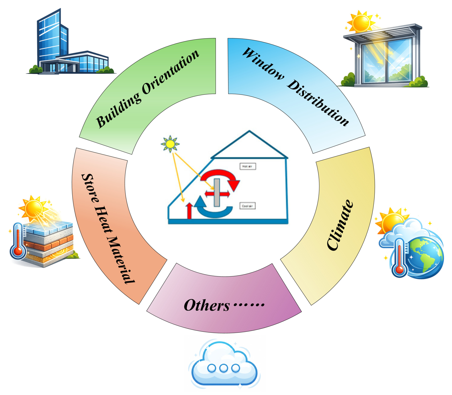
As summarized in Figure 2, passive shading performance is not determined by shading length alone. It results from the combined effects of building orientation, window distribution, regional climate, thermal mass, envelope thermal performance, indoor functional requirements, and control/evaluation boundaries. Therefore, shading design should be assessed through multiple objectives, including solar-heat-gain reduction, overheating mitigation, mechanical cooling reduction, daylight availability, and glare control [20,21,30].

Despite these advances, several gaps remain. Many conventional designs still rely on summer or winter solstice noon solar angles and therefore cannot represent annual and daily variations in solar path or dynamic meteorological boundaries. Some studies treat daylighting, glare, thermal response, and operational energy use separately, while cross-climatic comparisons between hot low-latitude and cold high-latitude contexts remain limited. In addition, the role of thermal inertia may reverse across climates: it can stabilize indoor temperature in cold regions but may intensify heat accumulation in hot regions [31,32]. These gaps indicate the need for an early-stage passive shading optimization framework that is physically transparent, parameter-efficient, and transferable across climatic contexts as a complement to established simulation platforms.

To address these challenges and strengthen the role of passive solar shading as an integrated sustainable building strategy, this study develops and validates a lightweight, interpretable light–thermal–energy coupling framework for passive solar shading optimization in both existing-building retrofits and new construction. The framework integrates solar geometry, the Perez anisotropic sky model, building-surface irradiance calculation, indoor ray tracing and voxel-based illuminance distribution, DGP assessment, and a 6R3C (6-Resistance, 3-Capacitance) transient thermal network into a continuous computational chain linking outdoor solar radiation, indoor daylighting, thermal-mass heat storage/release, and operational energy consumption [33,34,35]. It evaluates 120 design combinations by varying shading scale, glazing performance, envelope thermal resistance, and thermal mass, with energy use, thermal response, daylight availability, and DGP control as measurable objectives.

The main contribution of this paper is not to replace EnergyPlus, TRNSYS, Radiance, or their combined workflows, but to provide a transparent decision-support method for early-stage design. Specifically, the framework (1) traces the causal relationship between shading geometry, solar path, indoor light spots, thermal-mass response, and energy use; (2) integrates daylighting, glare, transient thermal behavior, and operational energy in one modeling chain; (3) compares retrofit and new-construction strategies in hot low-latitude and cold high-latitude regions under the same evaluation logic; and (4) identifies the climate-dependent, and sometimes opposite, effects of thermal mass, thereby providing actionable guidance for passive shading, envelope retrofits, and low-carbon operation.

From a sustainability perspective, climate-adaptive passive shading can reduce operational energy demand and support reductions in associated carbon emissions, while targeted retrofit improves the performance of existing building envelopes without requiring complete replacement. By jointly considering energy use, daylight availability, glare, and thermal response, the framework also ensures that environmental benefits are not pursued at the expense of occupant comfort and well-being.

2. Theoretical Basis and Research Framework

This study is grounded in passive solar design, solar-radiation transfer, daylighting assessment, photothermal decoupling, transient thermal-network modeling, and multi-objective building-performance optimization [31,32,33,34,36]. The framework explains how outdoor solar radiation enters the building envelope, is redistributed indoors as daylight and solar heat gain, is stored or released by thermal mass, and is ultimately reflected in heating and cooling energy demand. Unlike simplified solstice-based shading rules, it supports full-day and full-year performance prediction under dynamic climatic boundary conditions.

The modeling chain first uses solar-geometry calculations and the Perez anisotropic sky model to characterize solar elevation, azimuth, direct normal irradiance (DNI), diffuse horizontal irradiance (DHI), and global horizontal irradiance (GHI). Building-surface irradiance is then converted into indoor daylight and solar-heat inputs through ray tracing and voxel-based illuminance mapping, while glare is quantified by DGP. Finally, a 6R3C transient resistance-capacitance network simulates indoor air temperature, envelope temperature, and internal thermal-mass response. This chain integrates shading geometry, glazing performance, envelope thermal resistance, and thermal mass into a unified optimization framework.

Two contrasting climatic boundary cases were selected to test the framework. Phoenix Sky Harbor International Airport, AZ, USA (approximately 33.43° N, 112.00° W; elevation 339–346 m), represents a hot, dry, cooling-dominated low-latitude case and corresponds to ASHRAE Climate Zone 2B. Its July average maximum temperature is approximately 41 °C, the December average minimum is approximately 8 °C, and average daily shortwave solar radiation ranges from about 3.2 to 8.4 kWh/m²/day, with an annual total of approximately 2128 kWh/m². These features make it suitable for examining defensive shading strategies that suppress excessive solar heat gain.

Fort Wainwright–Ladd Army Airfield, Alaska, USA (approximately 64.84° N, 147.60° W; elevation about 137 m), represents a cold inland high-latitude case with a long heating season, low winter solar altitude, large seasonal daylight variation, and substantial heating demand. The January average minimum temperature is approximately −27 °C, while the June–July average maximum is approximately 24 °C. In this context, passive shading must control summer overheating and glare without excessively reducing useful winter solar heat gain and daylight.

These sites are used as contrasting physical boundary cases rather than as statistical representatives of all hot and cold climates. Accordingly, the numerical optima reported in this paper are site-specific, whereas the underlying mechanisms and optimization logic are intended to be transferable. For other cities, the same framework can be applied by replacing the local EPW/TMY meteorological file, latitude, ground albedo, envelope properties, and building-use assumptions.

The Typical Meteorological Year (TMY) data were obtained from publicly available EPW databases, including the Ladybug Tools EPW Map and Climate.OneBuilding.org. The files provide 8760 hourly records of dry-bulb temperature, relative humidity, wind speed and direction, DNI, DHI, GHI, ground reflectance, and sky-condition information. These data define the dynamic outdoor boundary conditions for solar-radiation modeling, daylighting calculation, surface irradiance estimation, and transient thermal simulation; seasonal ground reflectance was additionally considered in the cold high-latitude case to represent snow effects.

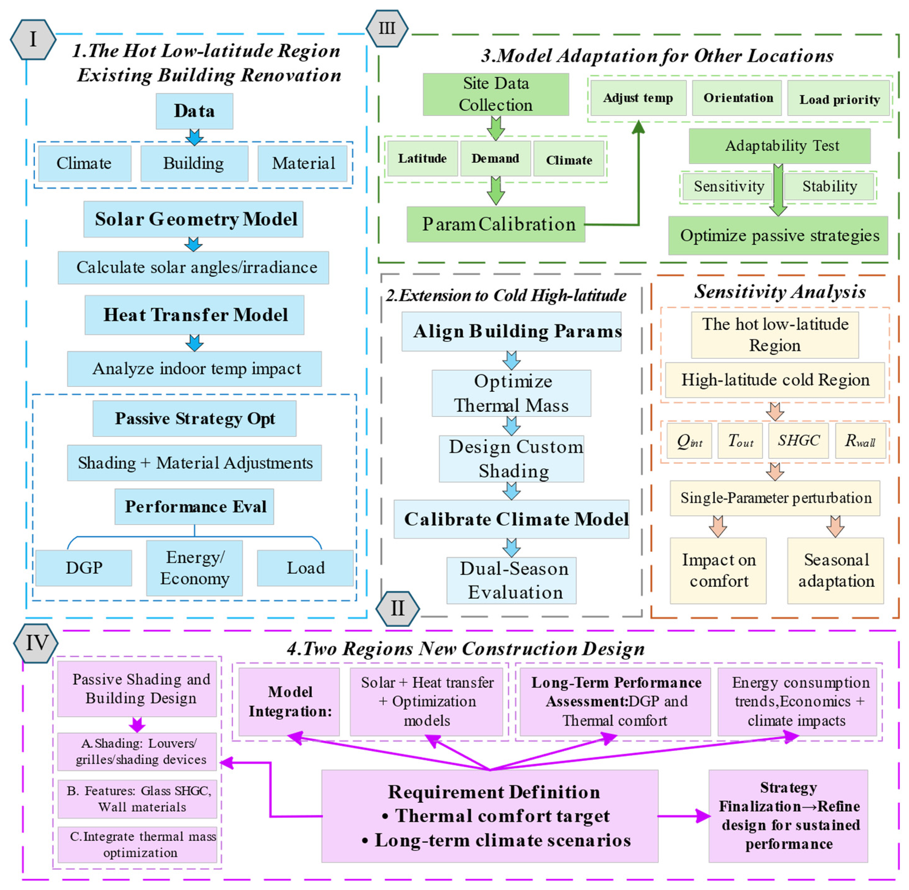
As shown in Figure 3, the framework contains four connected modules. Module I optimizes existing-building retrofits in hot low-latitude regions; Module II transfers the same logic to cold high-latitude regions by adjusting climatic, thermal-mass, and seasonal-evaluation settings; Module III tests adaptability through key parameters such as latitude, outdoor temperature, building orientation, internal heat load, solar heat gain coefficient (SHGC), and wall thermal resistance; and Module IV applies the calibrated framework to new-building design. Together, the modules connect retrofit analysis, climatic adaptation, sensitivity verification, and new-construction optimization within the same light–thermal–energy coupling logic.

Based on the above theoretical foundation and research framework, this study addresses the following research questions:

RQ1: What differences exist between hot, low-latitude regions and cold, high-latitude regions in terms of solar geometry, seasonal radiation characteristics, and climatic boundary conditions? How do these differences influence passive shading design?

RQ2: How can solar radiation, indoor daylighting, glare risk, the transient response of thermal mass, and building energy consumption be integrated into a coherent and interpretable light–thermal–energy coupling framework?

RQ3: Under substantially different climatic conditions, how should shading scale, glazing performance, building envelope thermal resistance, and thermal mass be jointly optimized for the retrofitting of existing buildings and the design of new buildings?

RQ4: Does thermal mass play different, or even opposite, roles in hot and cold regions? How does this influence the selection of passive shading and building envelope strategies?

RQ5: To what extent can the proposed framework be generalized to other climatic regions by substituting local TMY meteorological data and adjusting key physical parameters?

3. Methods and Data

3.1. Passive Solar Shading Illuminance Model

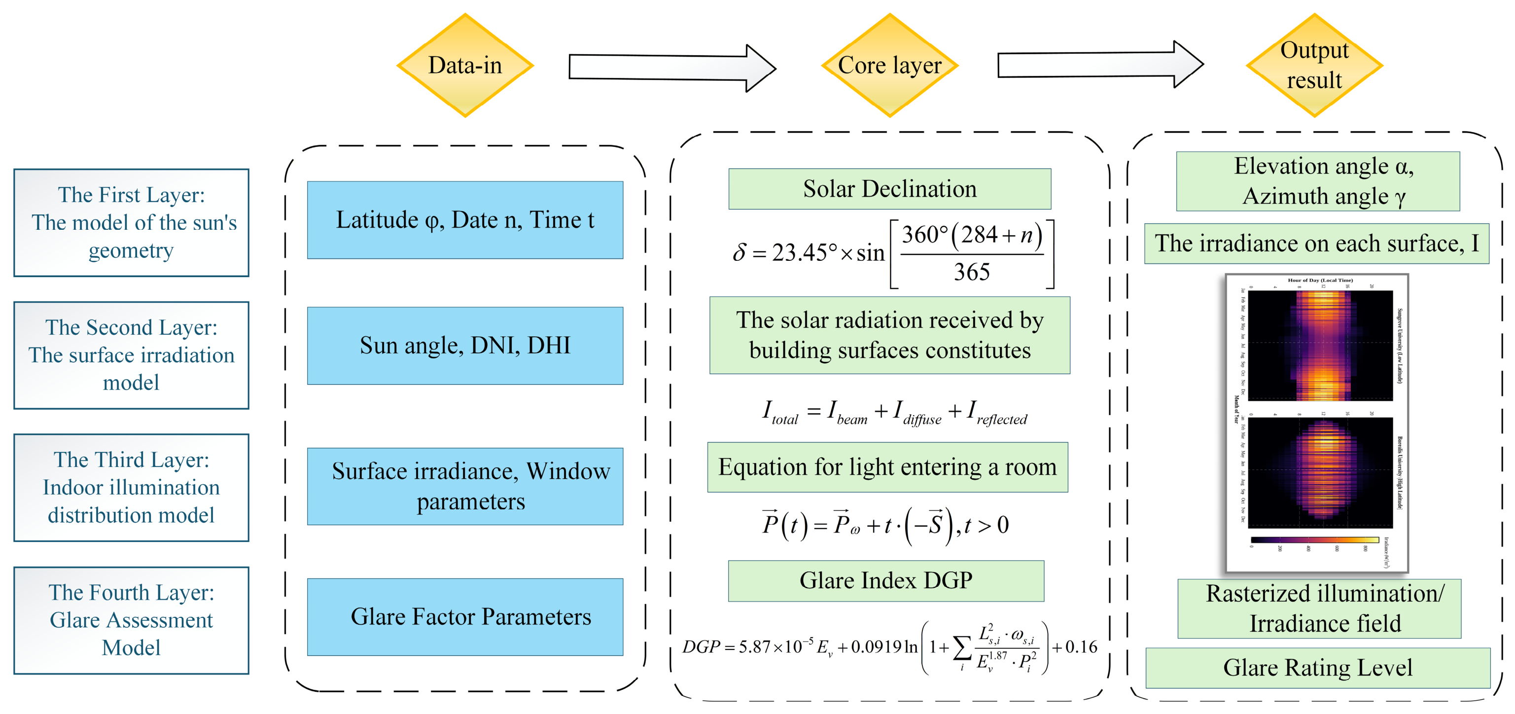
Due to the limitations of traditional shading strategies, which are based solely on the solar altitude angles at noon during the winter and summer solstices. This study developed a hierarchical solar radiation modeling system to characterize building features (Figure 4), with a core focus on accurately predicting the spatiotemporal distribution of solar radiation within buildings. The model employs a layered coupled architecture to calculate solar radiation intensity on building surfaces, spatial distribution of indoor illumination, glare risk metrics, and data required for thermal conduction modeling—providing critical basic data for subsequent shading strategy optimization.

Specifically, the model is divided into four layers. The first layer calculates solar geometric parameters based on latitude, date, and time. The second layer converts meteorological radiation data, including DNI and DHI, into irradiance received by different building surfaces. The third layer combines surface irradiance with window parameters to simulate indoor light transmission and gridded illuminance distribution. The fourth layer uses DGP-related parameters to evaluate glare risk. Together, these four layers provide a clear visual summary of the complete computational chain, from data input and core optical modelling to the final output results.

In this workflow, the “Data Input” section provides key input variables, including latitude, time, solar radiation, surface irradiance, window parameters, and glare-related coefficients. The “Core Layer” then calculates solar declination, solar altitude and azimuth angles, building surface irradiance, transmitted indoor light, and the DGP index. The “Output Results” section includes solar elevation and azimuth angles, irradiance on each building surface, gridded indoor illuminance/irradiance fields, and glare-rating levels. Therefore, Figure 4 serves as a methodological schematic of the daylighting model and provides the optical boundary conditions for the subsequent 6R3C transient thermal model and passive shading optimization.

Given the significant differences in solar paths between hot low-latitude regions and cold high-latitude regions, this hierarchical model achieves cross-scenario transferability by simply modifying latitude $\varphi$ and climate parameters ${\rho }_g$. This scalability enables the model to address current renovation challenges while providing robust design guidance and performance evaluation for future buildings.

3.1.1. Coordinate Systems and Spatial Discretization

Before establishing the coordinate system and spatial discretization, this study defines a representative classroom-type educational building as the geometric prototype for the optical and thermal simulations. The building is simplified as a two-storey rectangular teaching block with an east–west length of 60 m, a north–south width of 24 m, a floor height of 3.5 m, and a baseline orientation angle of 0°. A typical classroom module is defined as 10 m × 8 m. The south-facing window-to-wall ratio is set to 45%, while the window-to-wall ratio for the other orientations is set to 30%. The baseline glazing is represented by double low-emissivity glazing, with visible transmittance ${\tau }_{vis}$ = 0.65, solar heat gain coefficient SHGC = 0.45, and thermal transmittance $U_g$ = 2.0 W/m²∙K. These parameters are used as the reference optical and thermal boundary conditions for the subsequent solar radiation, daylighting, and transient thermal simulations.

These dimensions are not intended to reproduce a specific school building, but rather to provide a controllable and representative educational-building prototype. The selection of the two-storey layout, elongated plan form, floor height, orientation, and classroom module is informed by common commercial reference-building modelling practices, including the U.S. DOE Commercial Reference Building Models developed by NREL, PNNL, and LBNL. In these reference models, school buildings are included as representative commercial building types, and building-form parameters such as floor area, number of storeys, aspect ratio, floor height, orientation, window fraction, and internal mass are used as standard model inputs.

Therefore, the adopted geometric setting balances educational-building representativeness, modelling simplicity, and computational efficiency, while supporting the comparative analysis of solar penetration, glare risk, thermal response, and passive shading performance under hot, low-latitude and cold, high-latitude climatic conditions.

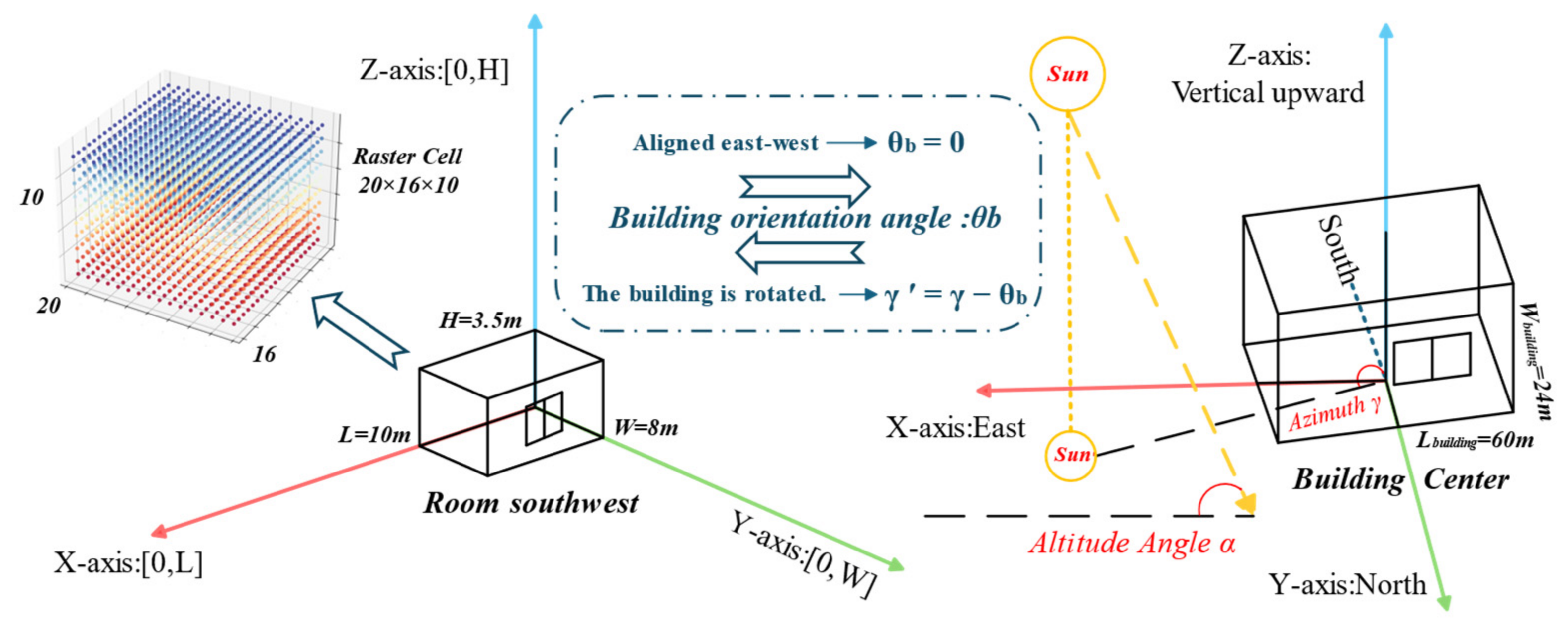
To establish a geometric relationship between solar motion and internal energy distribution within buildings, this study constructs a dual-coordinate coupling system, as shown in Figure 5.

Global Celestial Coordinate System: With the building center as origin, a right-handed coordinate system is established comprising true east (x-axis), true north (y-axis), and vertical upward (z-axis), defining solar altitude angle $\alpha$ and azimuth angle $\gamma$.

Building Interior Coordinate System: Using the southwest corner of a typical room ($10 \mathrm{m}\times 8 \mathrm{m}\times 3.5 \mathrm{m}$) as the origin, transformations are achieved through the building’s orientation ${\theta }_b$ angle (${\gamma }^{\prime }=\gamma -{\theta }_b$).

To obtain high-resolution indoor optical and thermal data, the interior space is discretized into $20\times 16\times 10$ grid cells using the voxel method, with each cell measuring $0.5 \mathrm{m}\times 0.5 \mathrm{m}\times 0.35 \mathrm{m}$. The center point of each grid cell stores the illuminance $E_{ijk}$, irradiance $G_{ijk}$, and glare probability $DG{P}_{ij}$ at that moment, providing refined spatial parameters for subsequent transient thermal conduction calculation and performance analysis.

3.1.2. Solar Geometric Position Model

To address the challenges of temporal variation and geographical disparity, this model calculates the dynamic relationship between solar position and building energy performance. It first employs Spencer’s method to compute the solar declination angle, reflecting the annual cyclical movement of the sun’s zenith point between the Tropics of Cancer and Capricorn:

$$\delta =23.45°\times \sin \left[{\displaystyle \frac{360°\left(284+n\right)}{365}}\right]$$

(1)

Calculate the solar hour $t_{solar}$ (Formula (3)) incorporating the longitude correction $\omega$:

$$\omega =15°\times \left(t_{solar}-12\right)$$

(2)

$$t_{solar}=t_{s\tan dard}+{\displaystyle \frac{\left(\lambda -{\lambda }_{ref}\right)}{15°}}+E_t$$

(3)

Subsequently, the solar altitude angle $\alpha$ (Formula (4)) and azimuth angle $\gamma$ (Formula (5)) are calculated using spherical trigonometry, and the direction of the solar path is corrected based on the sign of the hour angle $\omega$ (Formula (6)).

$$\sin \alpha =\sin \varphi \cdot \sin \delta +\cos \delta \cdot \cos \omega$$

(4)

$$\cos \gamma ={\displaystyle \frac{\sin \delta \cdot \cos \varphi -\cos \delta \cdot \sin \varphi \cdot \cos \omega }{\cos \alpha }}$$

(5)

$$\gamma =\left\{\begin{array}{l}-\left|\gamma \right|,\omega <0\left(\mathrm{In} \mathrm{the} \mathrm{morning}, \mathrm{the} \mathrm{sun} \mathrm{is} \mathrm{low} \mathrm{in} \mathrm{the} \mathrm{east}\right)\\ +\left|\gamma \right|,\omega >0\left(\mathrm{In} \mathrm{the} \mathrm{afternoon}, \mathrm{the} \mathrm{sun} \mathrm{was} \mathrm{setting}\right)\end{array}\right.$$

(6)

Finally, it is converted into a unit direction vector pointing toward the sun (Formula (7)), serving as the basis for subsequent calculations of surface irradiance and direct sunlight spot tracking:

$$\overrightarrow{S}=\left(\begin{array}{c}-\cos \alpha \cdot \sin \gamma \\ -\cos \alpha \cdot \cos \gamma \\ \sin \alpha \end{array}\right)$$

(7)

The model fully adapts to the solar motion characteristics of extreme climatic regions: $\alpha \le 0$ at night, there is no direct solar radiation. For hot low-latitude regions, the solar altitude angle at summer noon can approach 90°; for cold high-latitude regions, even at summer noon, the altitude angle remains relatively low, with long-duration oblique solar radiation, forming completely different solar radiation boundary conditions for building shading design.

3.1.3. Building Surface Irradiance Model

This layer implements the conversion from “solar radiation” to “building heat gain,” serving as a critical input for thermal load assessment.

Each exterior surface of the building is described by its normal vector $\overrightarrow{n}$: ${\overrightarrow{n}}_{south}=\left(0,-1,0\right)$ is the south wall, ${\overrightarrow{n}}_{north}=\left(0,+1,0\right)$ is the north wall, ${\overrightarrow{n}}_{east}=\left(+1,0,0\right)$ is the east wall, ${\overrightarrow{n}}_{west}=\left(-1,0,0\right)$ is the west wall, and ${\overrightarrow{n}}_{roof}=\left(0,0,+1\right)$ is the roof. The angle between the solar ray and the surface normal $\theta$ is the angle of incidence. Since the solar direction vector $\overrightarrow{S}$ is defined as pointing from the ground toward the sun, the ray propagation direction is $-\overrightarrow{S}$, and the cosine of the angle of incidence is:

$$\cos \theta =\overrightarrow{S}\cdot \overrightarrow{n}$$

(8)

The surface normal vector points outward from the building. When $\cos \theta >0$, the surface faces the sun and receives direct solar radiation; otherwise, no direct solar radiation is present.

Solar radiation received on building surfaces consists of three components: direct irradiance $I_{beam}$, diffuse irradiance $I_{diffuse}$, and ground-reflected irradiance $I_{reflected}$.

$$I_{total}=I_{beam}+I_{diffuse}+I_{reflected}$$

(9)

(1)

Direct irradiance is the projection of direct sunlight onto an inclined surface:

$$I_{beam}=\left\{\begin{array}{l}DNI\cdot \cos \theta ,\mathrm{if} \cos \theta >0 \mathrm{and} \alpha >0\\ 0, \mathrm{otherwise}\end{array}\right.$$

(10)

DNI represents direct normal irradiance, obtained from TMY meteorological data [29].

(2)

Diffuse irradiance employs the Perez anisotropic sky model, which accounts for the non-uniform distribution of sky brightness, including the annular region around the Sun and the brightening effect near the horizon:

$$I_{diffuse}=DHI\cdot \left[\left(1-F_1\right)\cdot {\displaystyle \frac{1+\cos \beta }{2}}+F_1\cdot {\displaystyle \frac{a}{b}}+F_2\cdot \sin \beta \right]$$

(11)

The meanings of the parameters in Equation (11) are presented in

Table 1. The meaning of each parameter in Equation (11).

Parameters	Description	Parameters	Description
DHI	Diffuse horizontal irradiance	$\beta$	Surface inclination angle
F1	Ring Brightness Coefficient	$a=\max \left(0,\cos \theta \right)$	Angle factor for facing the sun
F2	Horizon Brightness Coefficient	$b=\max \left(0.087,\cos \alpha \right)$	Horizontal Sun Angle Factor

.

The Perez model precisely simulates the distribution of diffuse light during cloudy $\epsilon$ or overcast conditions $\mathrm{\Delta }$ in the cold high-latitude region through parameters of sky clarity and sky brightness [37]. It defines eight sky types based on these parameters [35], as shown in

Table 2. Perez sky scattering radiation model coefficient table.

Sky Type	Parameter Vector V
Overcast with thick clouds	[−0.008, 0.588, −0.062, −0.060, 0.072, −0.022]
Overcast with thin clouds	[0.130, 0.683, −0.151, −0.019, 0.066, −0.029]
Cloudy	[0.330, 0.487, −0.221, 0.055, −0.064, −0.026]
Partly cloudy	[0.568, 0.187, −0.295, 0.109, −0.152, −0.014]
Partly Cloudy	[0.873, −0.392, −0.362, 0.226, −0.462, 0.001]
Clear	[1.132, −1.237, −0.412, 0.288, −0.823, 0.056]
Very clear	[1.060, −1.600, −0.359, 0.264, −1.127, 0.131]
Extremely clear	[0.678, −0.327, −0.250, −0.156, −1.377, 0.251]

, and performs calculations using the corresponding Perez coefficients:

$$\epsilon ={\displaystyle \frac{\left(DHI+DNI\right)/DHI+5.535\times {10}^{-6}\cdot {\theta }_z^3}{1+5.535\times {10}^{-6}\cdot {\theta }_z^3}}$$

(12)

$$\mathrm{\Delta }=DHI\cdot {\displaystyle \frac{m}{I_0}}$$

(13)

$$F_1=\max \left(0,f_{11}+f_{12}\mathrm{\Delta }+f_{13}{\theta }_z\right)$$

(14)

$$F_2=f_{21}+f_{22}\mathrm{\Delta }+f_{23}{\theta }_z$$

(15)

where ${\theta }_z=90°-\alpha$ is the solar zenith angle, m is the optical air mass, and I₀ is the normal irradiance outside the atmosphere (approximately 1367 W/m²). Let the sky brightness distribution parameter vector be denoted as $V=\left[f_{11},f_{12},f_{13},f_{21},f_{22},f_{23}\right]$.

(3)

Ground-reflected irradiance: For colder regions at higher latitudes across the globe, the model incorporates seasonal ground reflectance ${\rho }_g\left(m\right)$ (Equation (16)), with the ground-reflected component calculated as per Equation (17):

$${\rho }_g\left(m\right)=\left\{\begin{array}{l}0.75,m\in \mathrm{Snow} \mathrm{Months}\left(\mathrm{Nov}\text{-}\mathrm{Apr} \mathrm{for} \mathrm{Borealis}\right)\\ 0.20,\mathrm{otherwise}\end{array}\right.$$

(16)

$$I_{reflected}=GHI\cdot {\rho }_g\left(m\right)\cdot {\displaystyle \frac{1-\cos \beta }{2}}$$

(17)

GHI represents the global horizontal irradiance. This dynamic model captures the additional radiative gain from snow accumulation on building facades during winter, which is crucial for assessing indoor daylighting in cold high-latitude regions during the winter season.

3.1.4. Indoor Light Distribution Model

This layer bridges the transition from the “building envelope” to the “interior space,” tracking the projection location of each direct sunlight beam onto thermal mass. It provides the foundation for analyzing the “thermal flywheel” effect of floor thermal storage.

Windows serve as the primary pathway for solar radiation entering the interior. This study is based on the typical building envelope parameters of hot and cold regions; for windows located on walls $\omega$, they are parameterized, defining a set of parameters:

$$Windo{w}_j=\left\{\omega ,x_1,x_2,z_1,z_2,{\tau }_{vis}\right.,SHGC,\left.U_g\right\}$$

(18)

where $\omega \in \left\{\left.south,north,east,west\right\}\right.$ is the wall surface where the window is located; $\left(x_1,x_2\right)$ and $\left(z_1,z_2\right)$ represent the horizontal and vertical ranges, respectively; ${\tau }_{vis}$ is the visible light transmittance (0.6–0.75); SHGC is the solar heat gain coefficient (0.25–0.70); $U_g$ is the thermal transmittance coefficient of the glass (W/m²·K); and $A_w=\left(x_2-x_1\right)\times \left(z_2-z_1\right)$ is the window area [38,39,40].

The south-facing window-to-wall ratio of the building’s North is 45%, while other orientations are 30%. Taking the south-facing orientation as an example, the single-story height is 3.5 m and the wall length is 60 m, then:

$$A_{window,south}=0.45\times 60\times 3.5=94.5 {\mathrm{m}}^2$$

(19)

When sunlight enters a room, it forms light spots on the floor or interior walls. To track the distribution of direct light indoors, we employ a ray tracing algorithm to determine the position of these light spots. Light rays enter the room from any point $P_{\omega }=\left(x_{\omega },y_{\omega },z_{\omega }\right)$ on the window along the $-\overrightarrow{S}$ direction:

$$\overrightarrow{P}\left(t\right)={\overrightarrow{P}}_{\omega }+t\cdot \left(-\overrightarrow{S}\right),t>0$$

(20)

The intersection parameters and coordinates with the ground at z = 0 are given by Equations (21) and (22):

$$t_{floor}={\displaystyle \frac{z_{\omega }}{\sin \alpha }}$$

(21)

$${\overrightarrow{P}}_{floor}={\overrightarrow{P}}_{\omega }+t_{floor}\cdot \left(-\overrightarrow{S}\right)$$

(22)

If the point ${\overrightarrow{P}}_{floor}$ is within the indoor area $\left[0,L\right]\times \left[0,W\right]$, it receives direct light and maps it to the grid $\left(i,j,k\right)$$i=\left[P_{floor,x}/\mathrm{\Delta }x\right],j=\left[P_{floor,y}/\mathrm{\Delta }y\right]$. The direct irradiance of this grid is accumulated as:

$$G_{ij0}+=I_{beam}\cdot {\tau }_{vis}\cdot {\displaystyle \frac{\delta A_{\omega }}{A_{cell}}}$$

(23)

where $\delta A_{\omega }$ represents the window sampling element and $A_{cell}=\mathrm{\Delta }x\cdot \mathrm{\Delta }y$ denotes the grid area. Each grid cell stores illuminance, temperature, and glare probability. This high-resolution data preserves sufficient illuminance for analysis while the sunshade blocks heat.

Diffuse light enters from all directions and spreads nearly uniformly indoors, though it attenuates with distance. Using the split flux method, the diffuse light flux transmitted through windows is calculated as:

$${\mathsf{\Phi }}_{diffuse}=I_{diffuse}\cdot A_{\omega }\cdot {\tau }_{vis}$$

(24)

The diffuse illuminance at an indoor point $\left(x,y,z\right)$ is proportional to the visible solid angle from that point to the window. A distance attenuation model is employed:

$$E_{diffuse}\left(x,y,z\right)={\displaystyle \sum _j{E}_{0,j}\cdot f_{decay}\left(d_j\right)}$$

(25)

The reference illuminance directly in front of the window $j$ is denoted by $E_{0,j}$, the distance from this point to the window $j$ is denoted by $d_j$, the attenuation function is denoted by $f_{decay}\left(d\right)={\displaystyle \frac{1}{1+{\left(d/d_0\right)}^2}}$, and the characteristic attenuation distance is denoted by $d_0$.

Indoor illuminance arises not only from direct transmission but also includes contributions from multiple reflections off various interior surfaces. A simplified form of the radiometric method is employed for estimation. The reflectance values for each interior surface are listed in

Table 3. Reflectance of various surfaces indoors.

Ceiling (Light-Colored Paint)	Floor (Dark Tiles or Carpet)	Wall Surface (Medium Brightness)
${\rho }_c=0.8$	${\rho }_f=0.3$	${\rho }_{\omega }=0.5$

, while the average reflectance is given by Equation (26).

$$\overrightarrow{\rho }={\displaystyle \frac{{\rho }_c{A}_c+{\rho }_f{A}_f+{\rho }_{\omega }{A}_{\omega }}{A_c+A_f+A_{\omega }}}$$

(26)

Considering infinite reflections, the enhancement factor and final illuminance of indoor lighting are given by Equations (27) and (28).

$${\eta }_{reflection}={\displaystyle \frac{1}{1-\overrightarrow{\rho }}}$$

(27)

$$E_{total}=\left(E_{direct}+E_{diffuse}\right)\cdot {\eta }_{reflection}$$

(28)

For typical classroom parameters, $\overrightarrow{\rho }\approx 0.5$ then ${\eta }_{reflection}\approx 2$, meaning that interior surface reflections approximately double the illuminance, which is an indispensable factor for daylighting performance evaluation [39].

3.1.5. Glare Assessment Model

This layer focuses on “human perception,” employing the DGP metric [41] to ensure that optimizing sunshade length simultaneously satisfies three hard constraints: energy efficiency, thermal comfort, and visual comfort (DGP < 0.35). Proposed by Wienold and Christoffersen [42], DGP represents the probability of an observer experiencing uncomfortable glare, with values ranging from 0 to 1.

$$DGP=5.87\times {10}^{-5}{E}_v+0.0919\ln \left(1+{\displaystyle \sum _i\frac{L_{s,i}^2\cdot {\omega }_{s,i}}{E_v^{1.87}\cdot P_i^2}}\right)+0.16$$

(29)

where $E_v$ is the vertical illuminance (lux) at the observer’s eye position; $L_{s,i}$ is the Luminance (cd/m²) of the i-th glare source; ${\omega }_{s,i}$ is the solid angle (sr) corresponding to the glare source; $P_i$ is the position index, representing the glare source’s position within the field of view.

To achieve a more accurate evaluation, the model distinguishes between two types of glare sources. Window background brightness is calculated using diffuse reflection:

$$L_s={\displaystyle \frac{E_{window}\cdot {\tau }_{vis}}{\pi }}$$

(30)

When the sun is directly overhead, the solar photosphere’s luminance $L_s=L_{sun}\approx 1.6\times {10}^9 {\mathrm{cd}/\mathrm{m}}^2$ and solid angle ${\omega }_s={\omega }_{sun}\approx 6.8\times {10}^{-5}\mathrm{sr}$ are employed. Through ray tracing $R\left(t\right)=P_{eye}+t{\overrightarrow{V}}_{sun}$, the mechanism determines whether the sun is visible within the field of view, ensuring the DGP accurately reflects the saturated glare level (DGP = 1.00) [43].

Calculation of the solid angle formed by the window relative to the observer’s eye position:

$${\omega }_s={\displaystyle \frac{A_{window}\cdot \cos {\theta }_{view}}{d^2}}$$

(31)

where $A_{window}$ is the window area, ${\theta }_{view}$ is the angle between the line of sight and the window normal, and d is the viewing distance.

The position index P reflects the influence of a glare source’s position within the field of view on glare perception, calculated according to the Guth position index model:

$$P=e^{\left(35.2-0.31889\tau -1.22e^{-2\tau /9}\right)\sigma \times {10}^{-3}+21+0.26667-0.002963{\tau }^2}$$

(32)

where $\tau$ and $\sigma$ represent the horizontal and vertical angles of the glare source relative to the line of sight, respectively.

Glare levels are classified based on DGP values, as shown in

Table 4. DGP glare classification.

DGP Scope	Glare Level	Subjective Experience
<0.35	A	Imperceptible glare
0.35–0.40	B	Perceptible and acceptable
0.40–0.45	C	Disturbing
>0.45	D	Unbearable

. This model calculates grid DGP values at the working surface elevation and uses the area where DGP > 0.40 as the glare evaluation metric.

3.2. Non-Steady-State Thermal Environment Model

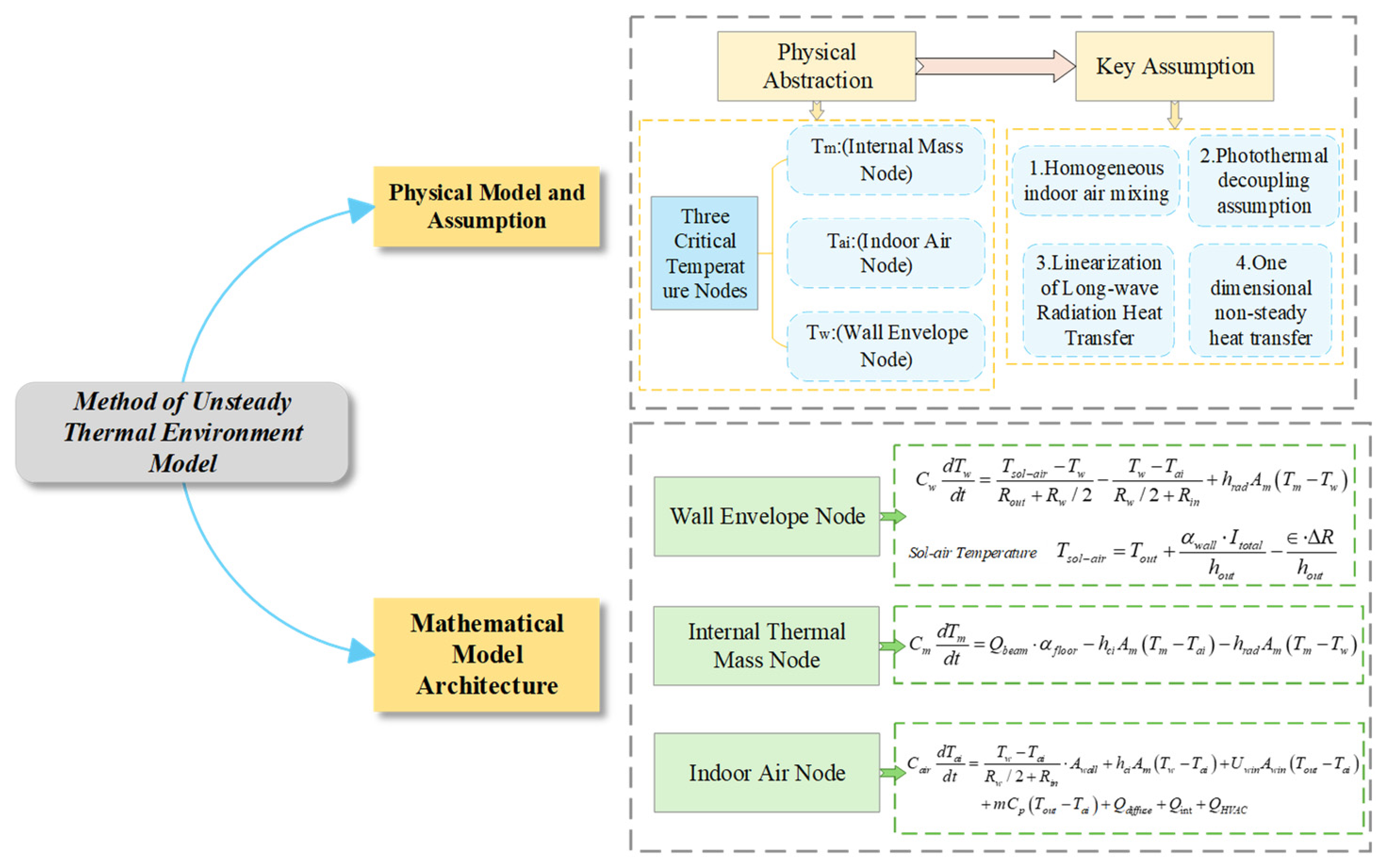
The above optical model realizes the refined simulation of solar radiation transmission and indoor light spot distribution. To further reveal the thermal regulation mechanism of passive shading and building thermal mass under different climatic conditions, especially to solve the seasonal contradiction between winter solar heat gain and summer overheating prevention in cold high-latitude buildings, this study constructs a transient indoor thermal environment model based on a 6R3C thermal resistance–thermal capacitance network. As illustrated in the framework of Figure 6, A 6R3C third-order dynamic thermal network model has been designed. Different from traditional steady-state thermal simulation models, this model regards building floors, walls, and other components as thermal mass carriers with obvious thermal inertia and quantifies the dynamic temperature regulation effect of thermal mass. It can accurately simulate the transient response of indoor temperature to external meteorological changes, envelope thermal inertia, and indoor heat sources, realizing refined evaluation of building thermal environmental performance under dynamic climatic conditions [44].

This framework consists of two main parts: the physical models and assumptions, and the mathematical model architecture. In the physical abstraction, the building thermal system is simplified into three key temperature nodes: the indoor air node ($T_{ai}$), the wall envelope node ($T_w$), and the internal thermal mass node ($T_m$). These nodes respectively represent the rapid thermal response of indoor air, the heat storage and heat transfer processes of the building envelope, and the heat storage and release behaviour of floor slabs, interior walls, and other internal thermal mass components.

The key assumptions include uniform mixing of indoor air, photothermal decoupling of solar radiation and heat transfer, linearization of long-wave radiation heat transfer, and one-dimensional transient heat transfer through the building envelope. Based on these assumptions, the mathematical model architecture establishes three coupled energy-balance equations for the wall envelope node, the internal thermal mass node, and the indoor air node. The wall envelope node receives an outdoor thermal driving force represented by the outdoor composite temperature, namely the Sol-air Temperature. The internal thermal mass node absorbs part of the transmitted direct solar radiation and exchanges heat with the indoor air and wall surfaces. The indoor air node comprehensively accounts for convective heat transfer, window heat transfer, ventilation and infiltration, diffuse solar gain, internal heat gain, and heating, ventilation, and air-conditioning (HVAC) loads. Therefore, Figure 6 visually illustrates how the optical output obtained from the previous solar radiation and daylighting model is converted into the transient indoor thermal response. It serves as a methodological bridge between the illuminance model and the subsequent energy-consumption optimization model.

3.2.1. 6R3C Thermal Network and Assumptions

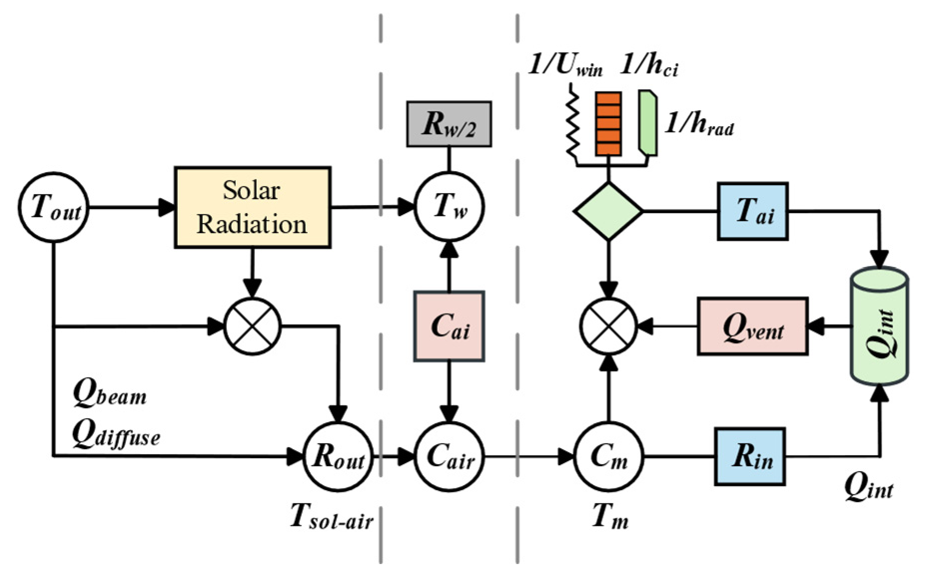
The building thermal system is abstracted into a lumped parameter network comprising thermal resistance (R) and thermal mass (C), as shown in Figure 7, including three core temperature nodes: $T_{ai}$, $T_w$, and $T_m$. The indoor air node has low thermal mass $C_{air}$ and responds rapidly to ventilation and indoor heat source changes; the wall envelope node has large thermal mass $C_w$, which can provides significant thermal inertia, buffering outdoor temperature fluctuations and solar radiation impacts; the internal mass node represented by floors and interior walls has moderate thermal $C_m$ storage capacity, and realizes heat exchange with indoor air and envelopes through radiation and convection, forming the core “thermal flywheel” effect of passive solar buildings.

Combined with the research objectives, the model adopts reasonable physical simplifications: indoor air is uniformly mixed in a single room; envelope heat transfer is simplified to one-dimensional unsteady heat transfer; long-wave radiation heat transfer is linearly processed; solar radiation is decoupled into direct and diffuse components; the photothermal decoupling assumption is adopted to simplify the different physical pathways through which transmitted solar radiation affects indoor thermal response. This assumption is supported by the solar-distribution logic used in established building simulation methods. In EnergyPlus, solar radiation entering a thermal zone through windows is explicitly divided into beam and diffuse components. For a simplified solar distribution, transmitted beam solar radiation is assumed to fall primarily on the floor, where it is absorbed according to the floor solar absorptance, while diffuse solar radiation is treated as a more spatially distributed short-wave gain over interior surfaces. Under more detailed solar-distribution settings, the beam component can be ray-traced onto different interior surfaces according to solar geometry and room configuration. Therefore, assigning the direct component mainly to the internal thermal mass node and treating the diffuse component as a distributed indoor heat gain is a reasonable reduced-order approximation for the 6R3C thermal network.

This treatment is also consistent with thermal-network modelling studies in which solar and internal heat gains are lumped into different thermal nodes, and heat storage is represented by thermal capacitances. Previous dynamic thermal-circuit models have shown that beam, diffuse, and reflected solar radiation can be distributed to interior zone surfaces according to solar geometry, façade orientation, and view-factor relationships. Since the present study aims to develop a lightweight and interpretable model for early-stage passive shading optimization, the direct solar component is assigned to the internal thermal mass node $T_m$, representing floors, interior walls, and other heat-storage surfaces, whereas the diffuse component is assigned to the indoor air node $T_{ai}$ as a spatially distributed gain after multiple reflections. which act on different thermal nodes respectively to realize refined photothermal coupling simulation.

3.2.2. Mathematical Model Architecture

The dynamic evolution of the model is described by the following three coupled ordinary differential equations (ODEs), corresponding to the conservation of energy at three nodes.

Figure 7 further illustrates the detailed energy-flow structure of the 6R3C thermal resistance–thermal capacitance network used in the transient indoor thermal model. In this network, the building thermal system is represented by three dynamic temperature nodes: $T_w$, $T_m$, and $T_{ai}$. Thermal resistances describe the heat-transfer paths between the outdoor environment, the building envelope, the internal thermal mass, and the indoor air, while thermal capacitances represent the heat-storage capacities of the wall envelope, indoor air, and internal thermal mass.

The left side of Figure 7 shows the outdoor thermal boundary, where the outdoor air temperature ($T_{out}$) and solar radiation are combined into the outdoor composite temperature, namely the Sol-air Temperature ($T_{sol-air}$), which serves as the external thermal driving force for the wall envelope node. Solar radiation entering the interior is decomposed into direct radiation ($Q_{beam}$) and diffuse radiation ($Q_{diffuse}$). The direct radiation component primarily acts on the $T_m$, while the diffuse radiation component contributes to the thermal balance of the $T_{ai}$. The right side of the figure represents the indoor heat-exchange processes, including window heat transfer, convective heat transfer, long-wave radiative heat transfer, ventilation/infiltration heat exchange ($Q_{vent}$), internal heat gain ($Q_{\mathrm{int}}$), and HVAC load ($Q_{HVAC}$). Therefore, Figure 7 visually demonstrates how solar radiation, envelope heat transfer, thermal storage and release by internal thermal mass, ventilation, internal heat gains, and HVAC control are coupled within the proposed transient thermal model. This provides the physical basis for subsequent energy-consumption calculation and passive shading optimization.

The wall absorbs the combined outdoor heat and transfers it indoors, while simultaneously exchanging long-wave radiation with the internal thermal mass:

$$C_w{\displaystyle \frac{d{T}_w}{dt}}={\displaystyle \frac{T_{sol-air}-T_w}{R_{out}+R_w/2}}-{\displaystyle \frac{T_w-T_{ai}}{R_w/2+R_{in}}}+h_{rad}{A}_m\left(T_m-T_w\right)$$

(33)

$$T_{sol-air}=T_{out}+{\displaystyle \frac{\alpha \cdot I_{total}}{h_{out}}}-{\displaystyle \frac{\in \cdot \mathrm{\Delta }R}{h_{out}}}$$

(34)

where $T_{sol-air}$ is outdoor composite temperature (Sol-air Temperature) combines the thermal effects of outdoor air temperature and solar radiation into a single equivalent temperature parameter, as shown in Formula (34).

This is the core carrier of passive solar heat utilization. Layers of material with a specific thickness and density, whose energy balance equations incorporate convective heat transfer and the absorbed heat from direct sunlight calculated in Section 3.1.4. This node absorbs direct solar radiation passing through the window, releases heat via convection and radiation, and simulates the absorption and release of heat by thermal mass:

$$C_m{\displaystyle \frac{d{T}_m}{dt}}=Q_{beam}\cdot {\alpha }_{floor}-h_{ci}{A}_m\left(T_m-T_{ai}\right)-h_{rad}{A}_m\left(T_m-T_w\right)$$

(35)

The energy balance for indoor air nodes includes wall convection, internal thermal mass convection, window conduction, ventilation air exchange, and internal heat sources:

$$C_{air}{\displaystyle \frac{d{T}_{ai}}{dt}}={\displaystyle \frac{T_w-T_{ai}}{R_w/2+R_{in}}}\cdot A_{wall}+h_{ci}{A}_m\left(T_w-T_{ai}\right)+U_{win}{A}_{win}\left(T_{out}-T_{ai}\right)+m{C}_p\left(T_{out}-T_{ai}\right)+Q_{diffuse}+Q_{\mathrm{int}}+Q_{HVAC}$$

(36)

The $Q_{diffuse}$ portion of diffuse solar radiation absorbed by the air, $Q_{\mathrm{int}}$ heat generated by occupants and equipment, and $Q_{HVAC}$ representing the thermal load of the temperature control system (positive values indicate heating, negative values indicate cooling). System energy consumption will be calculated by accumulating these values $Q_{HVAC}$ and dividing by the corresponding energy efficiency ratio.

3.2.3. Key Physical Mechanisms and Parameters

To accurately characterize the photothermal coupling difference of solar radiation in indoor thermal regulation, this study innovatively adopts a photothermal decoupling strategy:

$Q_{beam}$: Directional radiation assumed to pass through windows and strike the floor ($T_m$), causing floor heating followed by gradual air heating via convection. This simulates the thermal storage principle of passive solar rooms.

$Q_{diffuse}$: Non-directional, assumed to be absorbed by suspended particles or multiple reflections, directly contributing to thermal gains at the $T_{ai}$.

Combined with the rasterized solar spot data generated in Section 3.1, the model enables spatially localized heating rather than uniform heating. This addresses considerations regarding the impact of “solar prediction paths” on energy storage.

To evaluate a building’s passive thermal regulation capacity under extreme climates and the impact of active $Q_{HVAC}$ loads, this study sets the natural infiltration rate at 1.0 ACH. This simulates natural air leakage with doors and windows closed, preventing high ventilation rates from masking the thermal insulation properties of the building envelope. This approach accurately reflects heat accumulation effects within the interior. Additionally, the model accounts for occupant activity patterns, setting a 1200 W thermal load between 08:00 and 18:00 and 0 W during other hours to accurately track nighttime cooling processes.

3.3. Integrated Energy Conservation Optimization Model

Based on the above optical illuminance model and transient thermal environment model, this study constructs a multi-objective collaborative optimization model for passive shading strategies. In the selection of optimization technologies, considering the maintenance difficulty of louver dynamic adjustment and the instability of vegetation shading performance affected by growth cycles, four low-maintenance and high-reliability passive shading and envelope optimization technologies are selected. A total of 120 groups of design parameter combinations are traversed through the global grid search algorithm to obtain the optimal design schemes for existing building retrofits and new building constructions in different climatic regions.

The optimization objectives and constraints are as follows:

$$\min \left(E_{heating}+E_{cooling}+E_{lighting}\right)$$

(37)

$$DGP<0.45 \& Lux>Minimum$$

(38)

The baseline annual energy consumption was calculated using the proposed light–thermal–energy coupling model under the no-shading baseline scenario. Taking this baseline case as the internal reference, the energy-saving rate of each optimized design combination was then calculated and used as a benchmark for comparing the performance of the 120 design combinations.

3.3.1. Design Variables and Optimization Matrix

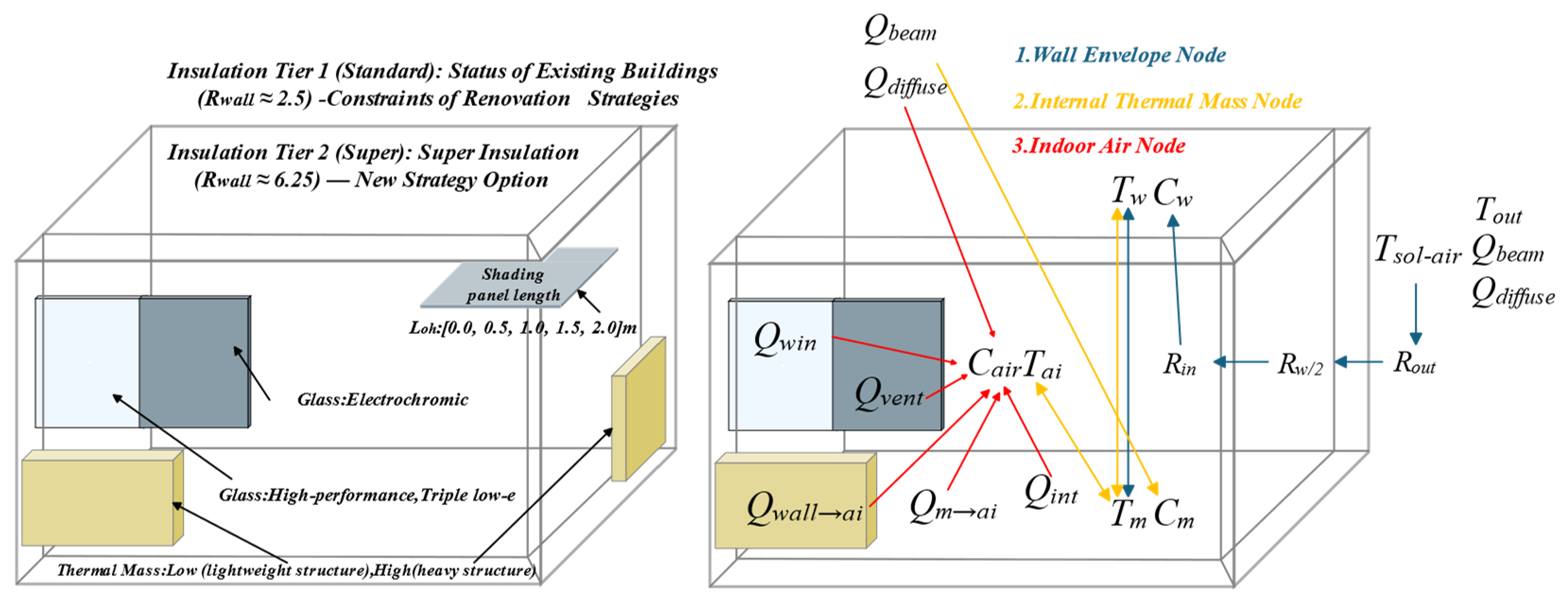
Figure 8 defines the physical decision space and energy transfer logic. The left diagram clarifies the physical constraint differences between “renovation” and “new construction” in Model 3. To distinguish the parameter differences and design restriction characteristics of existing building retrofits and new building constructions, this study expands the design decision space to 120 groups of parameter combinations, covering four core design variables: shading device length, glazing type, thermal mass grade, and envelope thermal insulation level.

The 120 design combinations were generated using a full-factorial experimental matrix rather than random sampling. Four design variables were included in this matrix: shading device length, glazing type, thermal mass level, and envelope insulation level. Among these variables:

Sunshade length $L_{oh}$ [0.0, 0.5, 1.0, 1.5, 2.0] m, balancing summer heat protection and winter daylight gain.

Glass types include standard, low-emissivity, tinted glass, plus high-tech electrochromic technology, high-performance double-silver low-emissivity glass, and triple-silver low-emissivity glass.

Thermal mass levels encompass lightweight structures like low-thermal-mass timber frames, gypsum board, and wooden floors, alongside heavyweight structures such as high-thermal-mass reinforced concrete slabs and solid clay.

Thermal insulation levels are categorized into two options: existing buildings retain their original brick facades with mineral wool cavity fill, achieving thermal resistance of $R_{wall}\approx 2.5$. New constructions feature super insulation using high-performance aerogel and vacuum insulated panels, requiring only 50 mm thickness to elevate thermal resistance to $R_{wall}\approx 6.25$.

Thus, the total number of combinations was calculated as (5 × 6 × 2 × 2 = 120). Each combination represents a possible passive shading and building envelope design strategy and was evaluated using the same light–thermal–energy coupling workflow. This full-factorial structure ensures that the effects of shading depth, glazing performance, thermal mass, and envelope insulation level, as well as their interactions, can be compared consistently. The use of such a parameter matrix is consistent with previous shading optimization studies, in which geometric shading variables, glazing properties, and building envelope parameters are commonly adjusted through parametric simulation and multi-objective evaluation to identify trade-offs among energy consumption, daylighting performance, glare control, and thermal comfort.

The section on the right of Figure 8 links these design variables to the transient thermal equilibrium model. It illustrates how outdoor temperature, Sol-air Temperature, $Q_{beam}$, $Q_{diffuse}$, window heat transfer ($Q_{win}$), $Q_{vent}$, $Q_{\mathrm{int}}$, and heat conduction between nodes are coupled through the wall envelope node, internal thermal mass node, and indoor air node. In this way, Figure 8 demonstrates how the abstract design variables in the optimization matrix are transformed into physical input parameters for the light–thermal–energy coupling model. The figure also clarifies the mechanisms through which shading devices, glazing systems, envelope insulation, and thermal mass jointly influence indoor thermal balance, HVAC loads, daylighting conditions, and glare control.

The glazing performance parameters include the SHGC, visible light transmittance (${\tau }_{vis}$), and thermal transmittance ($U_g$). These parameters are commonly used to characterise window energy performance. The thermal transmittance represents heat transfer through the glazing under non-solar temperature-driven conditions, while the SHGC describes the fraction of incident solar radiation transmitted into the indoor space through the window system.

The glazing performance parameters used in this study were selected based on typical values for low-emissivity (Low-E), tinted, electrochromic, and high-performance glazing systems, and were used as representative modelling inputs. The LBNL WINDOW program is widely used to calculate the U-value, SHGC, and visible light transmittance of complete window systems based on the properties of glazing layers and frame components. Its calculation algorithms are consistent with the procedures specified in ISO 15099 [45], NFRC 100 [46], and NFRC 200 [47]. Electrochromic glazing was modelled as a variable-transmittance system because electrochromic materials can dynamically adjust visible light transmittance, typically varying over a broad range between a low-tint state and a high-transmittance state.

The values in

Table 5. Key parameters for different types of glass.

Glazing Type	(Ug) W/m2·K	SHGC	(τvis)	Modelling Role
Standard double glazing	2.70	0.70	0.78	Conventional reference glazing
Double low-e glazing	2.00	0.45	0.65	Baseline reference glazing
Tinted glazing	2.40	0.35	0.40	Solar-control glazing with reduced daylight
Electrochromic glazing	1.80	0.14–0.47	0.15–0.60	Dynamic solar and glare control
High-performance double-silver low-e glazing	1.50	0.28	0.60	High-performance solar-control glazing
Triple-silver low-e glazing	1.20	0.22	0.50	High-insulation and low-solar-gain option

are representative modelling values rather than manufacturer-specific product data. They are used to distinguish the relative optical and thermal performance levels of the glazing alternatives in the full-factorial experimental matrix.

As shown in

Table 6. Specific heat capacity and thermal conductivity per unit volume for different levels of thermal mass.

Thermal Mass Level	Representative Construction	Thermal Conductivity (k) W/(m·K)	Density (ρ) kg/m3	Specific Heat (cp) J/(kg·K)	Volumetric Heat Capacity (ρcp) MJ/(m3·K)
Low thermal mass	Timber frame, gypsum board, lightweight floor	0.13–0.25	500–950	840–2000	0.8–1.0
High thermal mass	Reinforced concrete slab, clay brick, solid masonry	0.70–1.70	1700–2400	840–900	1.4–2.2

, the thermal mass parameters were defined according to typical material thermal-property ranges. The low-mass category represents lightweight assemblies such as timber framing and gypsum board, while the high-mass category represents concrete, brick, and masonry assemblies with greater heat storage capacity. The volumetric heat capacity ρc_p was used to represent the ability of each construction type to absorb and release heat. Typical material property databases report, for example, gypsum plasterboard with thermal conductivity around 0.16 W/(m·K), specific heat around 840 J/(kg·K), and density around 950 kg/m³; CIBSE guidance also gives representative conductivity values for gypsum plasterboard and timber.

3.3.2. Lighting Energy Consumption and Thermal Capacity Performance

Initial optimization favored 2.0 m sunshades. To correct this bias, we introduced seasonal lighting energy consumption: when winter indoor illuminance drops below 500 lux due to excessive shading, artificial lighting must be activated. This generates approximately 600 kWh/yr of additional energy. This constraint adjusted Fort Wainwright’s optimal shading length from 2.0 m to 1.5 m.

In addition, the model reveals the climate-dependent boundary of thermal-mass performance. In conventional passive solar design, high thermal mass is often considered beneficial because materials such as concrete, brick, and masonry can absorb daytime solar heat and release it later, thereby reducing indoor temperature fluctuation and potentially lowering heating demand. However, this mechanism depends on whether the thermal mass can receive sufficient useful solar gain during the day and whether the stored heat can be retained within a well-insulated envelope during the night. In the present cold high-latitude case, the winter solstice period provides only approximately 4 h of daylight and nearly 20 h of nighttime. Under such an extremely short-day condition, the available solar energy is insufficient to fully charge heavyweight internal mass, while the long night-time period increases the duration of heat dissipation and the morning preheating demand of massive components. As a result, the simulation indicates that, for this specific high-latitude winter boundary condition, high insulation combined with lightweight construction can outperform heavyweight high-thermal-mass construction in terms of annual energy use.

This finding should not be interpreted as a universal contradiction of passive solar design theory. Rather, it defines an applicable boundary: high thermal mass is beneficial when sufficient solar gain, appropriate exposure of mass, strong envelope insulation, and a compatible occupancy/heating schedule are available; however, in extremely high-latitude cold regions with very short winter daylight, low solar altitude, long night-time heat-loss periods, and limited winter solar charging, excessive thermal mass may increase heating energy demand. Therefore, the present result refines the conventional empirical design logic by identifying the conditions under which the benefit of thermal mass may be weakened or reversed.

4. Results

4.1. Solar Irradiance Characteristics and Passive Shading Implications

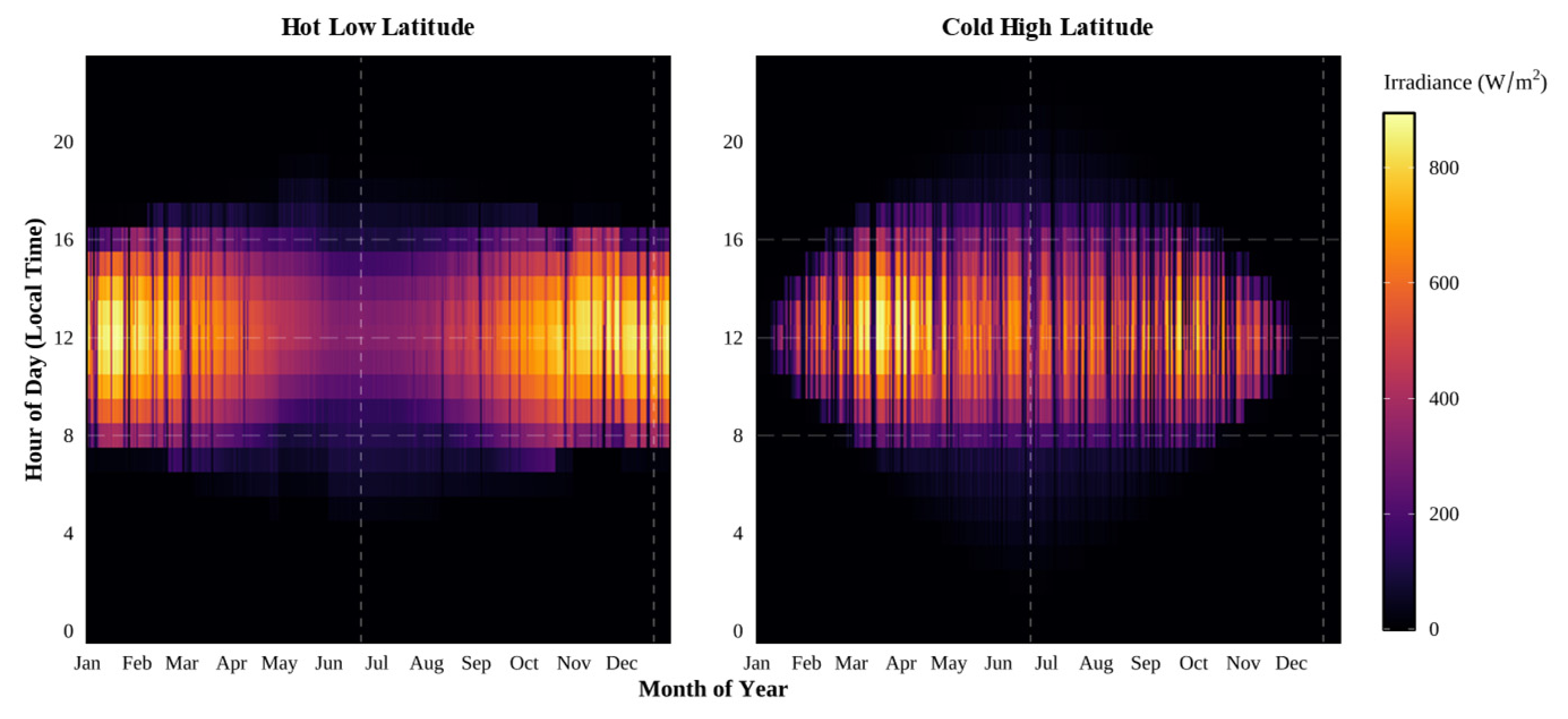
Figure 9 presents the annual vertical-plane solar irradiance heat maps for the hot low-latitude and cold high-latitude cases. The two dashed vertical lines indicate the summer and winter solstice periods, allowing the seasonal distribution of solar exposure to be compared directly. In the hot low-latitude case, vertical irradiance remains high and relatively continuous throughout the year. This indicates that the façade is exposed to persistent solar thermal stress and that passive shading must operate as a year-round solar-gain control strategy rather than as a seasonal accessory. Therefore, for this climatic condition, the primary function of shading is to reduce excessive direct solar penetration, suppress indoor overheating, and lower cooling demand.

In contrast, the cold high-latitude case shows a strongly seasonal irradiance pattern. The irradiance distribution is concentrated around the summer period, while winter irradiance and daylight duration are substantially reduced. This means that a shading device that performs well in summer may become detrimental in winter if it excessively blocks useful solar heat gain and daylight. Therefore, the cold high-latitude case requires a selective shading strategy: solar radiation should be controlled during summer and shoulder seasons, but useful winter solar gain should be preserved as much as possible.

These results indicate that the two regions should not be treated using a uniform shading rule. In the hot low-latitude case, the annual irradiance pattern supports a defensive strategy based on persistent solar exclusion and heat-gain suppression. In the cold high-latitude case, the seasonal irradiance pattern supports a selective strategy that balances summer overheating prevention, winter solar admission, glare control, and heating-energy reduction. This result provides the climatic basis for the subsequent optimization of shading length, glazing performance, envelope insulation, and thermal mass.

4.2. Transient Thermal Response and Model Validation

The transient thermal environment model was solved using the explicit fourth-order Runge–Kutta method. The hourly meteorological boundary conditions were linearly interpolated to generate continuous time-varying inputs, and a one-week pre-operation period was introduced to reduce the influence of initial thermal-state deviation. This numerical setup ensures that the simulated indoor air temperature, wall envelope temperature, internal thermal-mass temperature, and HVAC load can reach a quasi-periodic operating condition before formal evaluation.

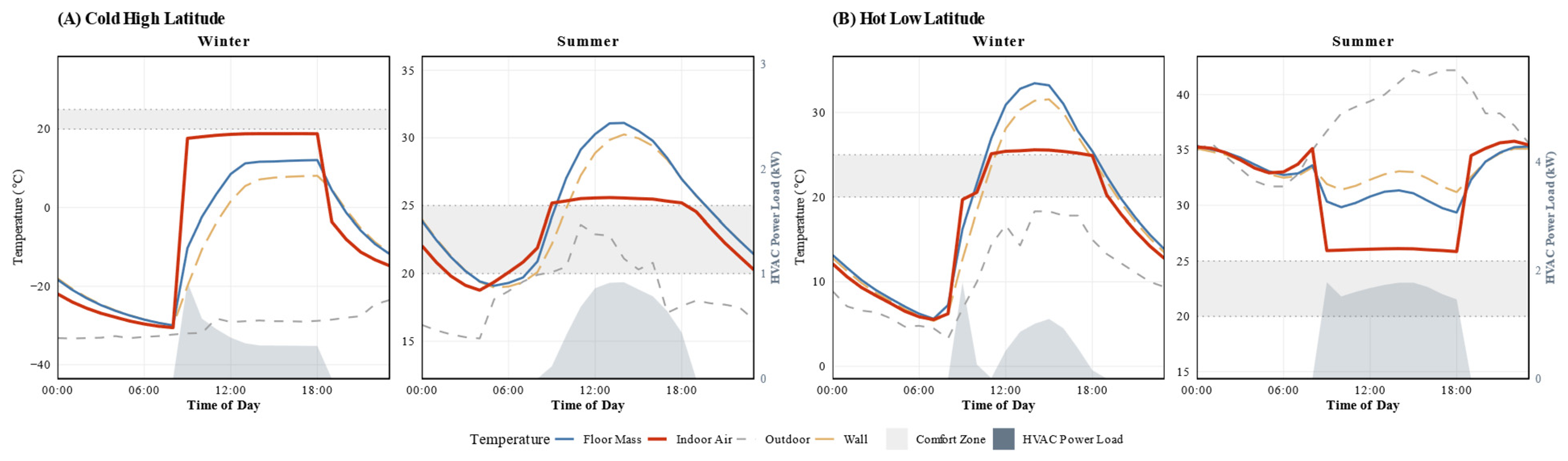
Figure 10 compares the dynamic evolution of indoor air temperature, wall temperature, internal thermal-mass temperature, outdoor temperature, comfort range, and HVAC load on representative winter and summer solstice days. In the cold high-latitude winter case, the outdoor temperature remains far below the comfort range, and the indoor thermal state is strongly dependent on envelope heat retention and limited daytime solar gain. The internal thermal-mass temperature rises during the daytime solar period and then decreases more slowly after sunset, indicating that the thermal-mass node can delay indoor temperature decline. However, the magnitude of this beneficial effect is limited by the short winter daylight duration.

In the hot low-latitude summer case, the indoor thermal-mass temperature remains higher than the indoor air temperature for an extended period. This indicates that part of the absorbed solar heat is stored in internal surfaces and later released back into the room, prolonging the cooling demand. The HVAC load curve follows the delayed release of stored heat, suggesting that excessive heat storage can become a secondary cooling burden under persistent high-temperature conditions. Therefore, Figure 10 confirms that the same thermal-mass mechanism can produce different outcomes under different climatic boundaries: it can buffer temperature decline in cold regions, but it can also extend heat accumulation in hot regions.

These results validate the physical consistency of the 6R3C transient thermal network. The model captures the delayed response between outdoor solar forcing, envelope heat transfer, internal thermal-mass storage, indoor air temperature, and HVAC load. This provides the thermal-response basis for the subsequent global grid-search optimization.

4.3. Optimization Results for Retrofit and New-Construction Strategies

4.3.1. Optimal Solution from Global Grid Search

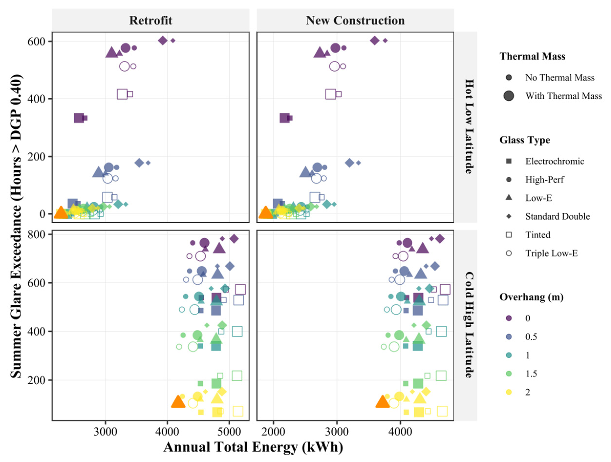
Through the full-factorial grid search of 120 design combinations and Pareto-frontier screening, the optimal passive shading and envelope strategies were identified for both retrofit and new-construction scenarios in the two climatic regions. The optimization considered annual energy consumption, glare control, daylight availability, and transient thermal response. As shown in Figure 11 and

Table 7. Optimal design strategy configuration table for existing building retrofits and new construction in different climate scenarios.

Location	Scene	Sun Visor Length	Glass Type	Thermal Mass
hot low-latitude	Renovation	2.0 m	low-Emissivity	Lightweight structure
	New	2.0 m	Triple-Silver Low-E	Heavy-duty structure
cold high-latitude	Renovation	1.5 m	Double-Silver Low-E	Lightweight structure
	New	2.0 m	Triple-Silver Low-E	Heavy-duty structure

, the optimal schemes are not determined by shading length alone, but by the coordinated effects of shading depth, glazing performance, envelope insulation, and thermal mass.

In the hot low-latitude retrofit scenario, the optimal strategy combines a 2.0 m external shading device, low-emissivity glazing, and a lightweight thermal-mass configuration. This shows that, under persistent high solar radiation, reducing transmitted solar heat gain is more important than increasing heat-storage capacity. Practical measures include adding high-reflectance external shading, using low-emissivity or electrochromic glazing, and avoiding heavy internal finishes that may store unwanted heat. In the hot low-latitude new-construction scenario, the optimal design combines 2.0 m external shading, triple-silver low-emissivity glazing, a high-performance envelope, and controlled heavyweight components. Deep shading and low-SHGC glazing should first suppress excessive solar gain, while heavyweight slabs or masonry should only be used after solar input has been effectively controlled.

In the cold high-latitude retrofit scenario, the optimal solution combines a 1.5 m shading device, double-silver low-emissivity glazing, and a lightweight structural system. The shorter shading depth helps preserve low-angle winter solar radiation; therefore, retrofit design should prioritize glazing insulation, glare control, reduced thermal bridging, and useful winter solar gain rather than maximum shading depth. In the cold high-latitude new-construction scenario, the optimal solution combines triple-silver low-emissivity glazing, a 2.0 m shading device, and heavyweight thermal mass within an improved envelope. High-performance glazing and super-insulated walls reduce heat loss, while protected internal thermal mass stores useful daytime solar heat; however, shading should be seasonally optimized to avoid blocking winter sunlight.

Overall, the global grid-search results indicate that passive shading should not follow a universal rule. Hot low-latitude regions require a defensive strategy based on deep shading, low-SHGC glazing, and heat-gain suppression, whereas cold high-latitude regions require a selective strategy that balances glare control, winter solar admission, envelope heat retention, and controlled thermal mass use [48].

4.3.2. Energy, Glare, and Daylighting Performance

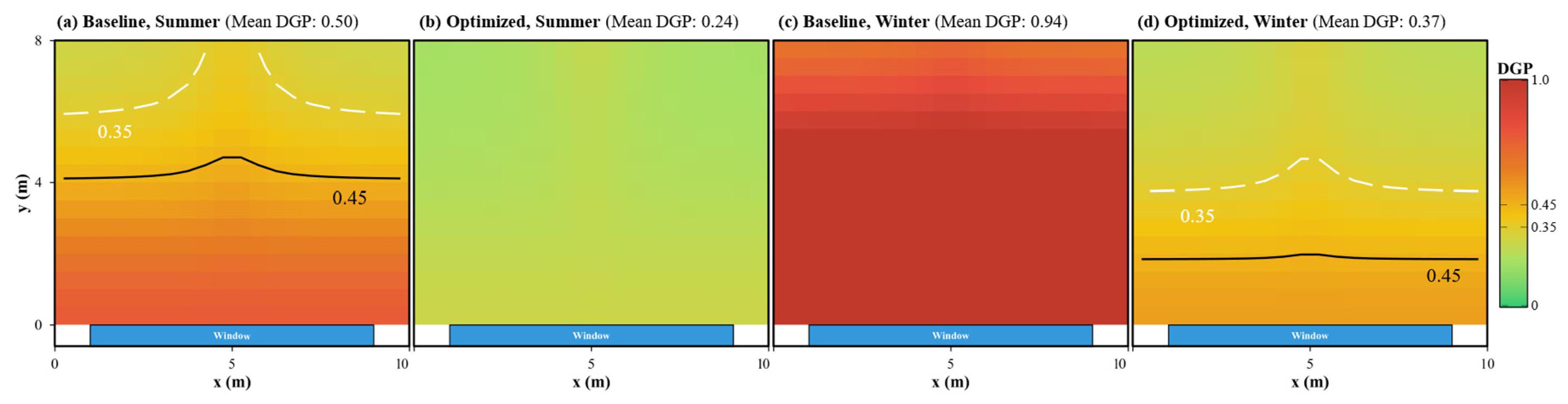
Figure 12 compares the indoor DGP distribution at the working-plane height of z = 0.75 m before and after optimization in the hot low-latitude case. Under the baseline condition, direct solar penetration produces severe glare. The mean summer DGP reaches 0.50, while the mean winter DGP reaches 0.94, indicating that glare risk is not limited to summer. In winter, the lower solar altitude allows direct sunlight to penetrate deeper into the room, producing extensive high-glare zones. After optimization, the mean summer DGP decreases to 0.24, and the mean winter DGP decreases to 0.37. This indicates that the optimized shading–glazing combination can suppress intolerable glare while still allowing useful daylight and winter solar gain.

Table 8. Two regions: design type-specific glare duration data table.

Hot Low-Latitude	Design Type	Glare Duration	Cold High-Latitude	Design Type	Glare Duration
Retrofit	Baseline	603 h	Retrofit	Baseline	782 h
	Optimized	0 h		Optimized	105 h
New	Baseline	603 h	New	Baseline	782 h
	Optimized	0 h		Optimized	105 h

further quantifies the annual glare-duration reduction. In the hot low-latitude case, annual glare duration decreases from 603 h in the baseline condition to 0 h after optimization. In the cold high-latitude case, glare duration decreases from 782 h to 105 h, corresponding to an 86% reduction. The remaining glare hours in the cold region mainly reflect the difficulty of controlling low-angle sunlight without sacrificing useful winter solar heat gain. Therefore, complete glare elimination is easier to achieve in hot regions, where solar exclusion is consistent with cooling-energy reduction, whereas cold regions require a more careful balance between glare reduction and winter solar availability.

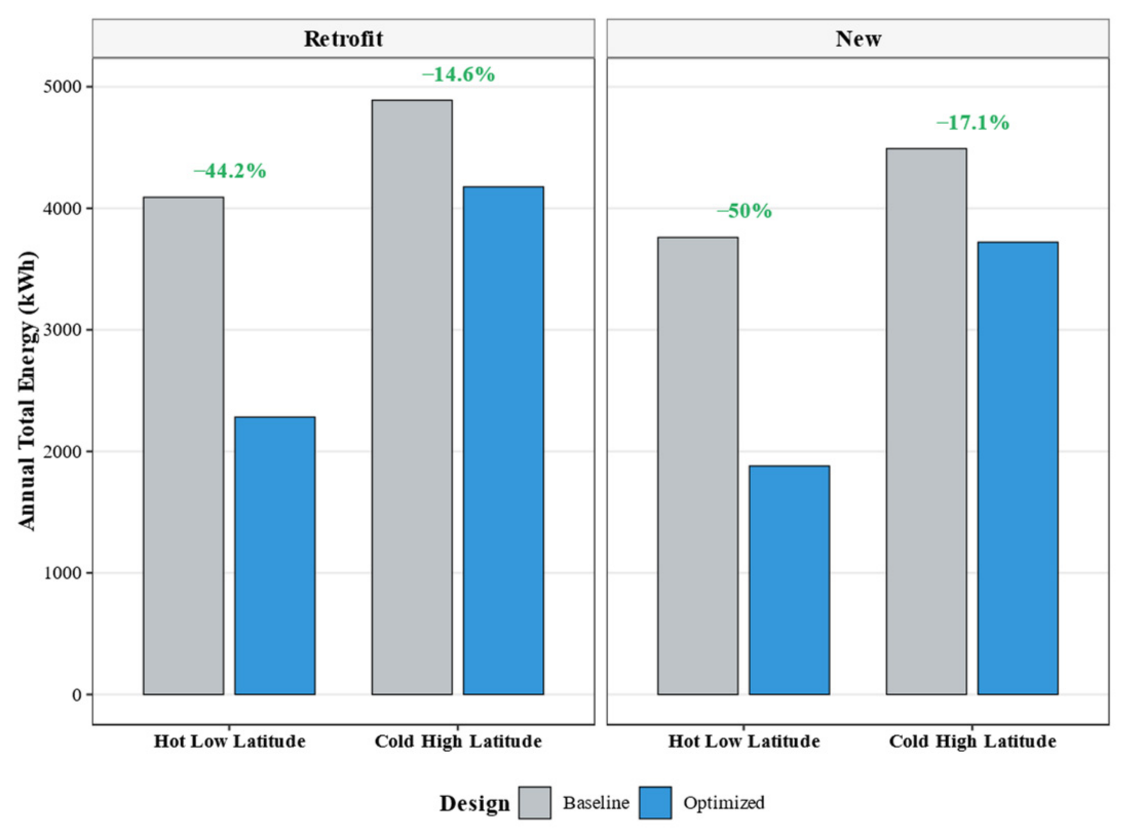
Figure 13 presents the annual energy consumption and energy-saving rates before and after optimization. In the hot low-latitude retrofit scenario, annual energy consumption decreases from 4091 kWh to 2282 kWh, corresponding to an energy-saving rate of 44.2%. This reduction is mainly caused by the combined effect of deep external shading and low-emissivity glazing, which reduces direct solar heat gain and lowers cooling demand. In the hot low-latitude new-construction scenario, the integrated use of deep shading, triple-silver low-emissivity glazing, and an improved envelope achieves an energy-saving rate of up to 50.0%.

In contrast, the energy-saving rate in the cold high-latitude region is lower, with 14.6% for retrofit and 17.1% for new construction. This does not indicate poor performance of passive shading. Rather, it reflects the fact that heating demand dominates in cold high-latitude climates, and excessive solar exclusion may reduce useful winter heat gain. Therefore, in cold regions, the optimized strategy contributes not only through energy reduction but also through glare control, daylight protection, and stabilization of indoor thermal response.

This regional difference fully reflects the climate adaptability characteristics of passive shading strategies and verifies the rationality of differentiated optimization design.

4.3.3. Temperature Optimization Analysis

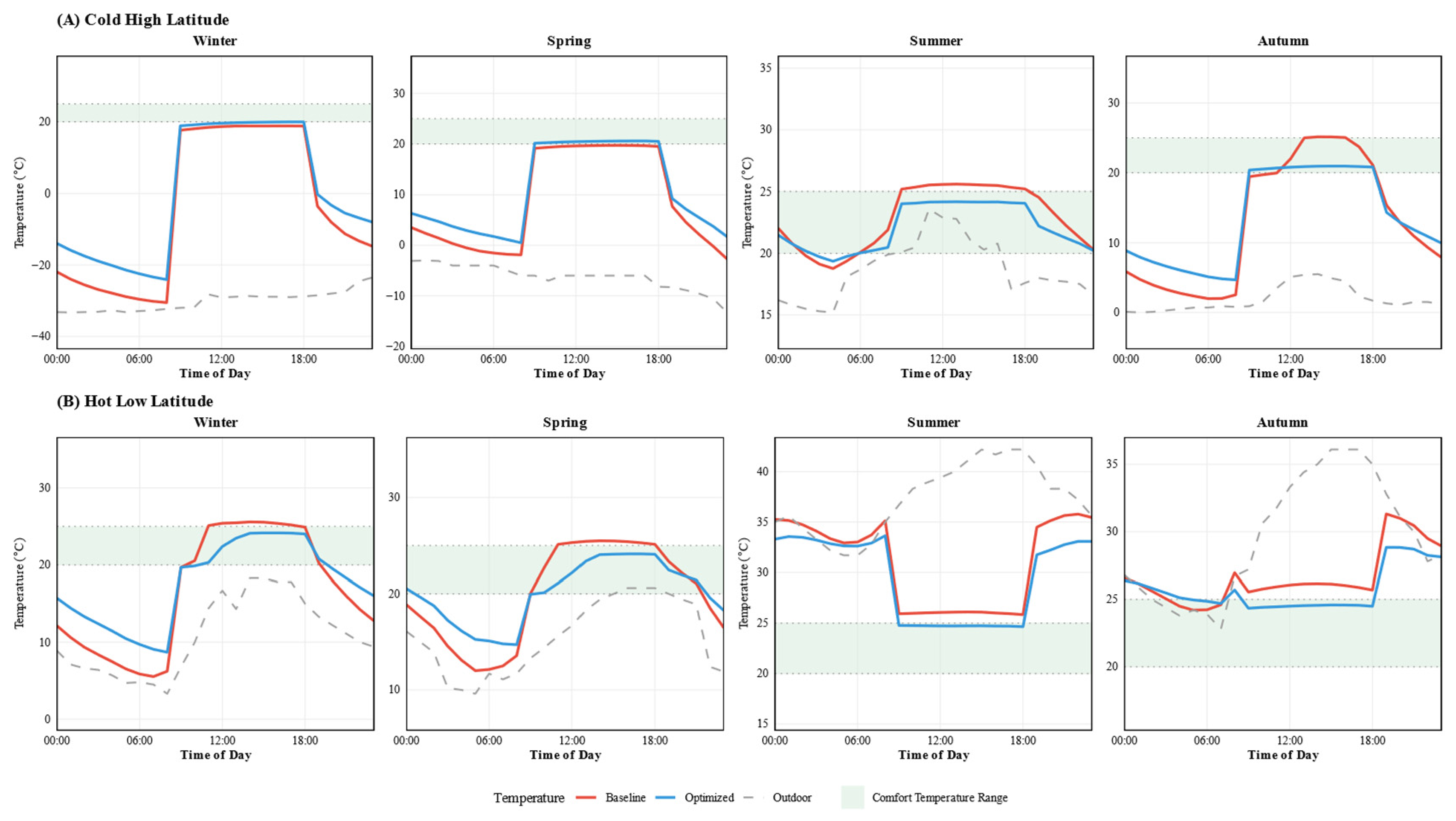
Figure 14 further compares the seasonal indoor temperature evolution before and after optimization. In the hot low-latitude region, the optimized configuration suppresses indoor overheating by reducing direct solar heat gain before it reaches the internal thermal mass. The indoor air temperature remains closer to the target comfort range during summer and autumn, while unnecessary solar heat accumulation in spring and winter is also reduced. This confirms that, for hot regions, the most effective passive strategy is not to increase heat storage capacity, but to reduce the amount of unwanted solar heat entering the room.

In the cold high-latitude region, the optimized solution shows a different mechanism. The super-insulated envelope reduces long-night heat loss, while controlled solar admission allows limited winter solar radiation to contribute to indoor heating. The thermal mass can delay temperature decline after sunset, but its benefit depends strongly on whether sufficient solar energy is available for charging during the short daytime period. Therefore, thermal mass in cold regions should be combined with high insulation and controlled solar access; otherwise, heavyweight walls may require additional preheating energy and increase total heating demand.

These temperature results clarify the climate-dependent role of thermal mass. Thermal mass acts as a thermal buffer only when its charging and discharging cycle matches the local solar and temperature rhythm. In hot low-latitude regions, where outdoor temperature and solar radiation remain high, stored heat is difficult to dissipate and may increase cooling load. In cold high-latitude regions, thermal mass can stabilize indoor temperature, but only if the envelope is sufficiently insulated and if winter solar gain is not excessively blocked. This finding refines the conventional assumption that “more thermal mass is always beneficial” in passive solar design.

5. Discussion

5.1. Climate-Dependent Mechanism of Passive Shading

The results confirm that passive shading performance is governed by climatic boundary conditions. In the hot low-latitude case, the annual vertical-irradiance pattern in Figure 9 indicates persistent solar exposure; therefore, deep external shading and low-SHGC glazing reduce cooling demand by preventing solar heat from entering the room. This explains why the 2.0 m shading solution appears in the Pareto-optimal set for both hot-region retrofit and new-construction scenarios. In the cold high-latitude case, irradiance is strongly seasonal, and winter solar availability is limited by short daylight duration and low solar altitude. Thus, excessive shading may block useful winter heat gain, which explains why the cold-region retrofit uses a shorter 1.5 m shading depth, while deeper shading is feasible in new construction only when combined with high-performance glazing, super insulation, and controlled façade design. This finding is consistent with shading-device reviews showing that performance depends on geometry, glazing, control strategy, climate, and multiple evaluation objectives rather than on a single energy metric.

5.2. Appropriate Model Transfer

Model transfer should be based on climatic thermal characteristics rather than latitude alone. Buildings at similar latitudes may have different energy and comfort needs because of humidity, cloudiness, diurnal temperature range, ground reflectance, wind exposure, and occupancy schedules. The proposed framework therefore uses location-specific EPW/TMY inputs and adjustable parameters, including DNI/DHI/GHI, albedo or snow reflectance, outdoor temperature, envelope properties, internal heat load, SHGC, wall thermal resistance, and thermal-mass level. By recalibrating these variables, the same modeling logic can support different climatic contexts, such as continental, maritime, high-altitude, arid, or humid coastal regions [49].

In this sense, the framework shifts passive shading design from simple geographic classification to climate-mechanism-based optimization. Hot regions generally prioritize full-year suppression of unwanted solar heat gain, while cold regions require a Pareto trade-off between heat-loss reduction, winter solar admission, daylight availability, and glare control.

5.3. Critical Interpretation of Thermal-Mass Effects

The most important physical insight of this study is that thermal mass is not universally beneficial. Conventional passive solar design often regards high thermal mass as advantageous because it can absorb daytime solar heat and release it later. The present results refine this assumption: thermal mass is helpful only when it can be sufficiently charged by useful solar gain and discharged during periods when heating is needed; it becomes problematic when it stores unwanted heat and releases it during cooling periods.

In hot low-latitude regions, persistent outdoor heat and strong radiation reduce the opportunity for night-time heat dissipation. Even with shading, internal mass may absorb transmitted solar heat and release it later, extending cooling demand. Therefore, the hot-region retrofit solution favors lightweight construction combined with deep shading and low-emissivity glazing. The priority is to prevent unnecessary solar heat from reaching the indoor thermal-mass node rather than to increase heat-storage capacity.

In cold high-latitude regions, thermal mass has a conditional role. It can delay temperature decline when winter solar gain is available, but at Fort Wainwright the very low solar altitude, approximately 4 h of winter daylight, and long nighttime heat-loss period limit solar charging and may increase preheating demand for heavyweight components. Thus, the cold-region retrofit favors lightweight construction and improved insulation, while heavyweight internal mass is more appropriate in new construction only when placed inside a high-performance envelope and supplied with controlled solar gain. This conclusion does not reject the value of thermal mass in all cold climates; instead, it identifies the boundary conditions under which its benefits may weaken or reverse.

5.4. Role of Building Orientation and Applicability to Other Orientations

Building orientation is an important boundary condition of the reported optima. The baseline model adopts an orientation angle of 0°, with a south-facing window-to-wall ratio of 45% and 30% on other façades. Orientation was not included as an independent variable in the 120-combination matrix because it is usually fixed in retrofit projects. Therefore, the reported shading depths and glazing strategies should be interpreted as reference-orientation results, while practical application to other orientations requires façade-specific adjustment.

South-facing façades are suited to horizontal overhangs because high-angle summer radiation can be blocked while part of low-angle winter radiation is admitted. East- and west-facing façades are more affected by low-angle morning and afternoon sun; therefore, vertical fins or wing panels are more suitable. For hot low-latitude cases, 0.5 m vertical louvers with low-emissivity glazing can reduce afternoon heat gain, whereas in cold high-latitude cases, 1.0 m vertical louvers with triple-silver low-emissivity glazing can combine glare control with heat-loss reduction.

5.5. Comparison with Existing Studies and Added Value of the Framework

The proposed framework is intended to complement, not replace, detailed platforms such as EnergyPlus, TRNSYS, and Radiance. These tools provide high-precision modeling of whole-building energy performance, daylighting, glare, and transient thermal processes, but they often require detailed model preparation, cross-platform exchange, and specialized expertise. The added value of this study lies in its lightweight and interpretable structure, which links solar geometry, indoor light distribution, DGP, thermal-mass response, and annual energy consumption in one transparent calculation chain.

Compared with existing shading-optimization studies, the framework adds value in two ways. First, the same 120-combination matrix is applied to both hot low-latitude and cold high-latitude cases, enabling direct comparison between contrasting climate mechanisms. Second, the optimal solutions are explained through physical processes such as direct solar penetration, internal heat storage, delayed heat release, glare risk, and heating/cooling demand. The framework therefore supports early-stage parameter screening and design interpretation before more detailed simulation is conducted.

The annual energy savings obtained from the simulations can also support preliminary economic screening when combined with local energy prices. However, feasibility depends on the costs of shading devices, high-performance glazing, envelope insulation, installation labor, structural reinforcement, maintenance, façade access, anchorage capacity, planning or aesthetic constraints, occupant disturbance, and long-term cleaning. Therefore, project-specific cost estimation and life-cycle economic assessment remain necessary before implementation.

These findings indicate that a sustainable shading strategy should not be selected on the basis of operational energy alone, but through an integrated balance among energy-saving and carbon-reduction potential, indoor environmental quality, technical feasibility, and life-cycle cost. The proposed framework can therefore function as an early-stage sustainability screening tool for identifying climate-appropriate solutions, although embodied carbon and full life-cycle impacts require further assessment.

5.6. Limitations and Broader Scientific Significance

Several limitations should be acknowledged. First, the 6R3C transient thermal network uses a single-node indoor air assumption. This reduced-order approach is appropriate for early-stage assessment of overall heating/cooling demand and average thermal response, but it cannot fully capture vertical air stratification, local thermal gradients, natural ventilation, infiltration, furniture layout, non-uniform solar patches, or occupant distribution. Future studies should couple the model with multi-zone airflow models, CFD simulations, or measured indoor temperature data. Second, the meteorological boundary conditions are primarily derived from historical TMY data. Although 8760-h TMY files are more representative than single design days or solstice assumptions, they cannot fully describe future extremes such as more frequent heat waves, cold spells, abnormal solar-radiation events, or prolonged still-air periods. Future work should therefore include climate-change scenario files, stochastic weather generators, and extreme-event stress tests. Despite these limitations, the study connects passive shading optimization with climate resilience through a transparent light–thermal–energy modeling chain. The results show that passive design should not be treated as a universal rule set; its effectiveness depends on the match among solar path, climate severity, orientation, glazing, insulation, thermal mass, and internal heat gains. The framework therefore extends passive shading research from energy-saving optimization toward climate-adaptive and low-carbon building design.

6. Sensitivity Analysis

To verify the reliability and parameter tolerance of the proposed optimization framework under multi-climate conditions and new building scenarios, single-factor sensitivity tests are carried out for four key parameters including outdoor temperature, indoor heat load, wall thermal resistance, and glass SHGC. The baseline values and fluctuation ranges for each parameter are shown in

Table 9. Sensitivity input parameters and variation range.

Parameter Name	Symbol	Reference Value	Low −	High +	Range of Variation
Internal heat load	$Q_{\mathrm{int}}$	1200 W	840 W (30%)	1560 W (+30%)	$\pm 30\%$
Temperature	$T_{out}$	EPW Data	−2 °C	+2 °C	$\left|\pm 2 °\mathrm{C}\right|$
Glass SHGC	$SHGC$	0.40	0.34 (−15%)	0.46 (+15%)	$\pm 15\%$
Wall R-value	$R_{wall}$	1.72 m2K/W	1.38 (−20%)	2.06 (+20%)	$\pm 20\%$

.

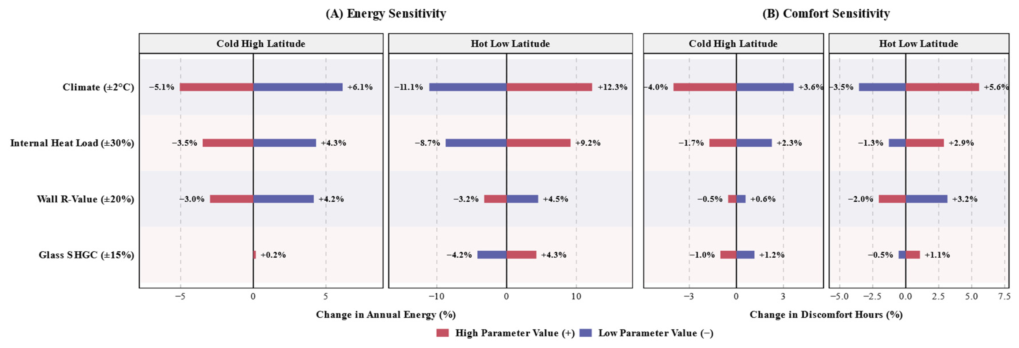
According to the energy sensitivity tornado diagram analysis in Figure 15A, a 2 °C temperature increase in the hot low-latitude region leads to a 12.3% surge in energy consumption, while a 2 °C decrease reduces energy consumption by 11.1%, demonstrating high sensitivity to temperature. In the cold high-latitude region, this sensitivity drops to 6.1%, indicating that colder regions exhibit more robust defense boundaries against extreme temperature fluctuations. Energy consumption fluctuations in the hot low-latitude region range from −8.7% to +9.2%. Internal heat dissipation significantly offsets passive shading benefits. In contrast, both glass SHGC and wall R-value impacts on energy consumption remain below 5%. This validates the proposed optimization strategy’s robustness, ensuring performance does not significantly degrade due to minor material aging or construction tolerances.

Analysis of discomfort hours (Figure 15B) reveals that in high-latitude regions, outdoor temperature exerts a greater influence on comfort levels (−4.0% to +3.6%) than in low-latitude areas. This indicates that passive design under extreme cold conditions must possess stronger seasonal adaptability. Glass SHGC exerts the least impact on comfort levels (fluctuating by approximately $\pm 1\%$). This demonstrates that physical solutions for geometric shading offer greater stability than chemical solutions involving glass coatings.

The four parameters selected for the sensitivity analysis were not intended to replace the main optimization variables, but to examine the robustness of the optimized passive solar shading strategies under representative climatic, operational, and envelope-performance perturbations. Outdoor temperature was selected because it directly represents the climatic driving force for heating and cooling loads. Internal heat load reflects variations in occupancy, equipment use, and other indoor heat gains, which may alter the transient thermal response of the room and the effectiveness of thermal mass. Wall thermal resistance represents the heat-transfer capacity of the opaque building envelope, while glass SHGC determines the amount of solar heat gain transmitted through the transparent envelope after the shading device has regulated incident solar radiation. Therefore, these four parameters are physically connected to the main design variables considered in this study, namely shading scale, glazing performance, thermal resistance of building envelopes, and thermal mass.

Full meteorological files, detailed material properties, infiltration rates, and occupant behaviour were not selected as independent sensitivity variables because the present framework is intended for early-stage, climate-adaptive design evaluation rather than field-calibrated operational prediction. The EPW/TMY meteorological file has already been used as the annual dynamic climatic boundary condition, including hourly temperature, solar radiation, humidity, wind, and sky-condition data. Detailed infiltration and occupant behaviour, by contrast, involve stochastic operational uncertainties and airflow interactions that are more appropriately addressed through field measurements, multi-zone airflow models, or CFD-based validation in future work. Thus, the selected sensitivity parameters provide a focused and interpretable way to test whether the optimized passive shading strategies remain stable under key climate, internal-load, and envelope-performance variations.

7. Conclusions

This study developed a lightweight and interpretable light–thermal–energy coupling framework for passive solar shading optimization in both existing-building retrofits and new-building design. The framework integrates solar geometry, the Perez radiation model, building surface irradiance calculation, indoor ray-tracing and voxel-based illuminance simulation, DGP glare assessment, and a 6R3C transient thermal network. By evaluating 120 design combinations, this study addressed two core questions: how shading geometry, glazing performance, envelope insulation, and thermal inertia should be adapted to hot low-latitude and cold high-latitude regions; and how their coupled energy, daylighting, glare, and thermal performance can be quantitatively evaluated.

The results show that passive shading strategies must be differentiated according to climatic boundary conditions. In the hot low-latitude region, persistent high solar radiation makes solar-heat-gain suppression the dominant design priority. The optimal retrofit solution combines 2.0 m external shading, low-emissivity glazing, and a lightweight structure, reducing annual energy consumption from 4091 kWh to 2282 kWh and achieving an energy-saving rate of 44.2%. For new construction in the same region, the combination of deep external shading, triple-silver low-emissivity glazing, improved envelope insulation, and controlled internal mass achieves an energy-saving rate of up to 50.0%.

In the cold high-latitude region, the design objective shifts from solar exclusion to selective solar control. Excessive shading may reduce useful winter solar gain and daylight availability; therefore, retrofit strategies should prioritize improved glazing, heat retention, and moderate shading. The optimized cold-region retrofit solution achieves an energy-saving rate of 14.6%, while the new-construction solution achieves 17.1% by combining high-performance glazing, super insulation, controlled thermal mass, and seasonally appropriate shading.

The visual-comfort results further demonstrate the effectiveness of the proposed framework. In the hot low-latitude case, the optimized strategy reduces mean summer DGP from 0.50 to 0.24 and mean winter DGP from 0.94 to 0.37. Annual glare duration decreases from 603 h to 0 h. In the cold high-latitude case, glare duration decreases from 782 h to 105 h, corresponding to an 86% reduction. These results show that the proposed method can reduce glare risk while maintaining useful daylight access, although cold high-latitude regions require a more careful balance between glare control and winter solar heat gain.

A key conclusion of this study is that thermal mass has a climate-dependent and conditional effect. In hot low-latitude regions, thermal mass may absorb excessive solar heat during the day and release it during evening or night periods, thereby increasing cooling demand. In cold high-latitude regions, thermal mass can stabilize indoor temperature only when sufficient solar gain is available and when the envelope is well insulated. Otherwise, heavyweight construction may increase preheating energy consumption and become an energy burden. Therefore, thermal mass should not be treated as universally beneficial; it must be matched with solar availability, envelope insulation, building-use schedule, and night-time heat-loss conditions.

Overall, this study provides a transparent decision-support method for early-stage passive shading and envelope design. Its contribution lies not in replacing established simulation platforms such as EnergyPlus, TRNSYS, and Radiance, but in offering an interpretable parametric framework that links shading geometry, solar path, indoor light distribution, thermal-mass behaviour, and operational energy consumption. Accordingly, this study contributes to sustainable development by providing a quantifiable decision-support tool for selecting passive measures that reduce operational energy demand, preserve indoor environmental quality, and enhance climate adaptability in both retrofits and new construction. Integrating this framework with future life-cycle carbon and cost assessments could further support environmentally and socio-economically informed low-carbon building decisions. Future work should further validate the model using measured data, include occupant behaviour and adaptive controls, and extend the framework to life-cycle carbon, construction cost, and stochastic future climate scenarios.