Climate-Sensitive Staged Predictive Framework for Sustainable Residential Retrofit Assessment Using Adaptable Base Model Templates

Abstract

Residential building retrofit requires reliable building energy simulation and efficient performance prediction. This research presents an adaptable workflow for establishing two residential base model templates, namely corner space (CS) and intermediate space (IS). The models were assessed through National Construction Code of Australia-based verification, comparison with a documented Melbourne residential reference model, and Morris index convergence analysis. These models were coupled with an AI-assisted three-stage prediction framework and evaluated across seven additional Australian climates, with Melbourne as the primary case, to examine cross-climate applicability. Stage 1 developed a two-variable analytical model to predict annual energy consumption. Stage 2 extended this to a three-variable relation and compared its energy predictions with support vector machine (SVM). Stage 3 examined multivariable cases using four machine learning (ML) models—artificial neural network (ANN), SVM, random forest (RF), and decision tree (DT)—to predict performance metrics and identify the best model. For the primary Melbourne case, the two-variable relation reproduced the simulated response with mean absolute percentage errors (MAPEs) of 0.27% and 0.62% for CS and IS, respectively. In Stage 2, the analytical model achieved a MAPE of 8.38%, while SVM reduced the error to 0.75%. Cross-climate results confirmed that the staged workflow remained robust across different climates. In Stage 3, SVM was robust with limited data, while the ANN and RF became more competitive with larger samples. DT was prone to overfitting. The proposed framework supports early-stage residential retrofit assessment by enabling retrofit hotspot screening and suitable surrogate model selection before detailed optimization.

1. Introduction

Buildings are responsible for approximately 36–40% of global energy usage and emissions [1,2]. Since existing buildings far exceed newly constructed ones, retrofitting is a crucial strategy that can reduce energy consumption by 30–72% [3,4]. Most retrofit studies utilized advanced physics-based simulations such as TRANSYS, jEPlus, IDA-ICE and EnergyPlus. These tools are largely applied to evaluate the performance of individual homes or established housing archetypes. Using these simulations, researchers can analyze how different retrofit strategies affect key factors, including energy consumption patterns, heating load, cooling load requirements, cost efficiency, and overall occupant comfort across various scenarios [5,6,7,8]. A recent study on a two-story house implemented retrofits such as wall and roof insulation, improved glazing, infiltration control, and shading, achieving a 38.8% reduction in energy consumption. Another study showed that similar retrofits combined with photovoltaic (PV) panels reduced thermal discomfort hours by 46% [2,9]. Furthermore, replacing the HVAC system alongside these strategies proved to be both effective and economical in lowering annual energy consumption [10]. In addition, retrofitting the building envelope and replacing lighting with LED lamps reduced operational energy use. Supplying electricity via PV panels further contributed to energy savings and lowered costs [11]. Recent studies also represent that retrofit assessment should consider indoor environmental quality. Ventilation strategies can affect indoor air quality, while climate responsive envelope solutions such as PCM can improve energy performance and thermal comfort [12,13].

Although physics-based simulations support retrofit analysis, they are computationally demanding, require detailed inputs and involve assumptions that add uncertainty. Therefore, many studies adopted statistical and machine learning (ML) techniques to improve the effectiveness of evaluations. These approaches, known as metamodels or surrogate models, can swiftly predict outcomes by learning from existing data [14,15]. A variety of metamodels, such as artificial neural networks (ANNs), support vector machines (SVMs), random forest (RF), Gaussian processes (GPs) and decision trees (DTs), are often employed to predict key energy-related metrics [16,17,18]. ANNs have been utilized prominently for modeling building energy and ensuring reliable predictions. It can effectively capture the nonlinear patterns of building energy data but requires adequate sampling to achieve reliable accuracy [19,20]. Moreover, an optimization framework has been employed recently on a case study building in northern China, with the help of a robust ANN model to identify optimal design schemes, and it was found that the workflow ran 38 times faster than the conventional approach [21]. Additionally, SVM and GP demonstrate satisfactory performance with the advantage of being supervised using fewer parameters. Nevertheless, SVM faces limitations when it comes to handling large-scale building energy analysis and high granularity [22]. Researchers have also implemented Latin hypercube sampling (LHS) to train an interpretable surrogate model like XGBoost, which helped to identify heating setpoint, airtightness, and equipment power density as dominant retrofit options of a Canadian single-detached house [23]. Furthermore, recent works have developed some data-driven frameworks where XGBoost, RF, and GBDT were utilized as the main predictors in the context of retrofitting, and the accuracy was reported as around R² ≈ 0.94 up to 0.98 [24,25,26].

However, the above discussed data-driven model reduce computation, yet multi-objective optimization (MOO) often handles the selection of retrofit measures. It is often considered as a way of choosing retrofit packages, balancing energy, comfort, and cost through Pareto searching [27,28]. Surrogate and metamodel-based approaches provided a fast performance, which enabled MOO techniques like NSGA-II/III to efficiently explore Pareto trade-offs over many retrofit options [29,30,31]. In contrast, the MOO process helped to generate a diverse design space that made the surrogate models more robust [32,33,34,35]. Although MOO and metamodels complement each other, there is a lack of a well-structured predictive pathway to guide practitioners in choosing a suitable prediction strategy based on problem complexity. Despite the above advances, residential retrofit applications remain limited to case-specific modeling [36]. Residential retrofit requires particular attention because the decisions are made under budget constraints, as the homeowners usually prefer a few retrofit options [37,38]. Since envelope-related parameters such as glazing, insulation, shading, etc., strongly affect building performance, representative residential spaces applicable across different housing forms can be used to identify retrofit hotspots [39].

Against this background, the present study addresses two research questions: (1) Can generic residential reference spaces be developed to represent common habitable spaces and support early identification of retrofit hotspots? (2) How should a staged prediction strategy guide the selection between analytical methods and machine learning surrogates when the number of retrofit variables increases? The underlying hypothesis is that generic base spaces can provide a generalizable foundation for residential retrofit analysis and enable early screening of retrofit hotspots across different climate conditions. Analytical relations may be sufficient and preferable when a small number of retrofit variables are considered, whereas a larger number of retrofit variables requires ML surrogates, selected through systematic comparison. However, modern simulation tools and AI platforms can assist retrofit analysis; they usually operate as application tools for a particular project or dataset. They do not, by themselves, resolve the two methodological issues identified above. Therefore, the aim of this study is to develop adaptable residential base model templates and to propose a three-stage prediction framework for pre-optimization of retrofit analysis, with additional cross-climate testing across multiple climate conditions. The next section identifies the key research gaps and clarifies the specific contributions of this study.

2. Research Gaps and Innovations

Upon reviewing the literature, it is evident that most retrofit studies are case-specific and their findings are difficult to transfer across residential space types, geometries, orientations and climatic conditions. Many recent studies have used ML models as surrogates for prediction, but they rarely explain whether a simpler analytical model may be sufficient for a small number of retrofit variables. They also do not clarify how to choose a suitable predictor when the number of variables increases. However, optimization studies often explore large combinations of retrofit measures, whereas real residential retrofit decisions are commonly limited to one or two interventions due to budget and implementation constraints. This means that complex predictive tools are not always necessary at the early decision stage. Therefore, this reality highlights the need for a fast, simple, and interpretable prediction framework that aligns with how retrofits are implemented.

To address the above gaps, this research developed two generic residential space templates, such as corner space (CS) and intermediate space (IS), representing common habitable spaces across detached houses, townhouses, and apartments. The study provides a commonly applicable space-level baseline that supports early screening of retrofit-sensitive zones. This space-level approach is important because retrofit-sensitive envelope features, such as windows, insulation, and many others, strongly influence building performance. Improving these features in a typical habitable space can provide a reasonable estimate of the energy use [40,41]. These spaces are also analyzed across eight orientations (0–315° at 45° steps), ensuring they cover all typical exposures and keeping the results widely applicable across various residential typologies. This study also proposes a three-stage predictive framework for retrofit analysis. Stage 1 shows that, when only two retrofit variables are considered, an analytical method can accurately predict annual energy consumption. Stage 2 extends this logic to a three-variable case and compares the analytical formulation with an ML model. In Stage 3, for more than three variables, an ML prediction strategy has been employed using several prominent ML models, providing a transferable prediction pathway when interactions are complex. Subsequently, the best-performing model is also identified. In addition, the proposed framework was examined across multiple Australian climate conditions to assess whether the prediction trends remained consistent beyond the primary Melbourne case.

The novelty of this work is that it introduces generic residential base model templates applicable beyond specific case studies and that can support early screening of retrofit hotspot zones. It also proposes an AI-assisted staged predictive strategy that selects the prediction method based on problem complexity, using interpretable analytical relations for simple retrofit decisions and ML surrogates for more complex scenarios. The framework is further evaluated across multiple climatic conditions, strengthening its applicability beyond a single case. Together, these contributions provide a reproducible pre-optimization framework for residential retrofit analysis. Accordingly, the purpose of this work is not to replace existing simulation or AI tools, but to provide a transferable framework for effective use in residential retrofit analysis. This reduces early modeling effort by helping practitioners quickly identify retrofit hotspots and prioritize cost-effective retrofit actions before detailed whole building analysis. It also provides a systematic pathway toward surrogate-based optimization.

3. Methodology

Residential buildings such as apartments and houses typically have spaces with one or two walls facing the exterior, while other surfaces are adjacent to other interior surfaces [42]. In building science, these spaces can be classified as corner rooms (two external walls) and intermediate rooms (one exterior wall). Moreover, the ceiling or roof also acts as an external boundary for single-story houses and upper floors of apartments. However, walls that are shared with other conditioned rooms are typically treated as surfaces with no heat transfer (adiabatic) [43,44,45]. Also, the literature indicated that an adaptable base model framework is necessary to quickly pinpoint the energy hot spots where retrofitting is essential [39,40]. Nevertheless, key envelope parameters, such as insulation levels, shading and window properties, significantly drive the results. Retrofitting these elements in a representative zone can effectively provide a good indication of building performance trends [41].

Based on the above criteria, we have modeled two generic residential spaces (Figure 1). The first one is a corner space (CS), where two walls (dark blue) and the roof (dark brown) are exposed to outside conditions and other walls are assumed as adiabatic (red). The second one is intermediate space (IS), with one wall (dark blue) and the roof (dark brown) exposed to outdoor conditions, and the remaining walls are considered adiabatic (red). For both CS and IS, the floor (light brown) is modeled as a ground-contact slab with constant ground temperature (annual average = 20 °C). The constant ground temperature of 20 °C was adopted following the NCC guidelines [46]. These spaces also represent common habitable rooms, such as bedrooms and living rooms in a residential space [42]. The room dimension for CS is 4 m in length, 4 m in width, and 2.7 m in height, while for the IS, the length and height are identical, while the width is 3 m. The green axis represents that both spaces are facing the north direction, and the window (light blue) is placed on the north-facing wall, where the window-to-wall ratio is taken as 30% (Figure 1). However, these base models were later analyzed for different orientations from 0° to 315° with 45° increments during the simulations. Therefore, the building rotates relative to true north, adjusting the window façade’s direction at each step. The role of these reference templates is to support rapid screening of retrofit sensitive zones before more detailed whole building simulation is conducted. Melbourne was presented as the primary climate case for detailed framework development, and to examine the broader applicability, these models were also evaluated under seven additional climate conditions of Australia.

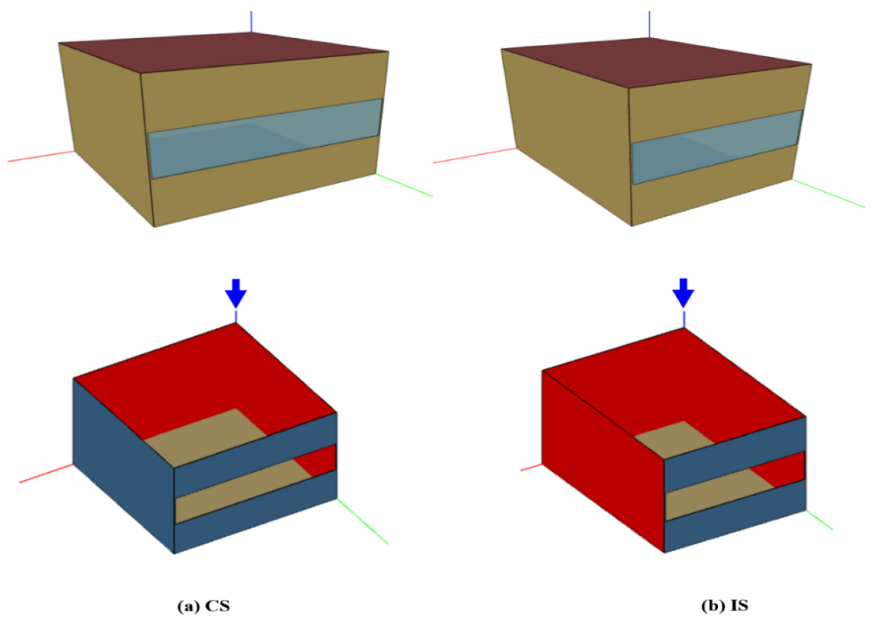
3.1. Modeling and Simulation Platforms

The building models were established in OpenStudio (v1.8.0), following the floor plan and using the key parameters listed in

Table 1. Base models’ characteristics.

Parameter	Description
Total floor area	16 m2 (CS), 12 m2 (IS)
Orientation	0°
Roof construction R-value	5.34 m2·K/W.
Wall construction R-value	3.40 m2·K/W
Floor construction R-value	2.46 m2·K/W
Glazing specification	U = 2.0 W/m2·K, solar heat gain coefficient (SHGC) = 0.25, visible transmittance (VT) = 0.50
Window-to-wall ratio (WWR)	30%
Heating setpoint	20 °C
Cooling setpoint	24 °C
Infiltration	Air changes/hour (ACH) = 0.75
Lighting	Lighting power density (LPD) = 4 W/m2
Equipment	Laptop = 2.5 W/m2
Occupancy	1 person (space/space-type)

. The input information and characteristics of the materials for the base models have been derived by following the guidelines provided by the National Construction Code (NCC) of Australia [46].

NCC suggests minimum total R-values for walls, roofs and floors based on the climate zone [46,47]. Accordingly, the base models were developed to satisfy the minimum NCC requirements for each corresponding climate condition. Australia has eight climate zones, ranging from Zone 1 tropical to Zone 8 alpine. The primary case, Melbourne, is situated in Climate Zone 6 and represents a temperate climate with warm summers and cool winters. The weather files of all climate conditions were used for simulation, as obtained from the repository of Climate.onebuilding.org [48]. Moreover, internal loads (lighting, occupancy and equipment) and their schedules of the base models were also assigned based on NCC guidelines to reflect realistic residential use patterns [46,47]. OpenStudio is an advanced modeling platform often implemented as the graphical interface for EnergyPlus, which has a limited graphical user interface and requires advanced expertise [8]. However, EnergyPlus is a highly validated and dependable tool for accurately simulating building energy performance. Therefore, jEPlus (v2.2.0) was employed as the simulation engine, as it is another powerful interface of EnergyPlus, which involves automated parametric runs and efficient dataset management [5,49]. Moreover, in this work, ideal air loads have been used to provide efficient heating and cooling in the designed space, which is a convenient feature that exists in EnergyPlus. In practice, this means the system will remove or add thermal energy to meet the zone’s setpoint conditions. It has been found that the predicted annual energy consumption of a building by the ideal air loads can be very similar to that of a real HVAC system [50,51,52].

3.2. Base Models’ Verification and Output Reliability Assessment

The reliability of base models were evaluated in three steps. As mentioned in Section 3.1, NCC guidelines were followed to develop the base models, which also recommend comparing simulation outcomes with the prescribed regulatory limits for verification [46]. Therefore, at first, the simulated outcomes such as heating load (HL) and cooling load (CL) were compared against the uniform national standard of NCC [46] for all climatic conditions. Secondly, since Melbourne was the primary climate condition, the outputs of Melbourne were compared with a residential reference model to examine the thermal response consistency. Lastly, Morris sensitivity analysis was also conducted across multiple sample sizes and climates. This approach is commonly utilized to represent that the model does not produce unreliable or random outputs [50,53]. It should be noted that the base models are generic reference templates, not monitored real buildings. Therefore, direct measured data validation was not applicable in this study.

According to NCC Clause S44C2, the maximum allowable HL and CL for a habitable space should be measured in MJ/m².annum and calculated by using the following formulas [46],

Heating load limit (HLL) = max (4, (0.0044 × HDH − 5.9) × F_H)

(1)

Cooling load limit (CLL) = (5.4 + 0.00617 × (CDH + 1.85 × DGH)) × F_C

(2)

Here, HDH = total annual heating degree hours for the building location, CDH = total annual cooling degree hours of the location, DGH = total annual dehumidification gram hours of the location, F_H = area adjustment factor of the HL, F_C = area adjustment factor of the CL.

The HDH, CDH, and DGH were calculated separately for each climate condition, using the corresponding hourly weather data from the weather files and the setpoints suggested by NCC (see Table 1). Moreover, if the habitable space in the model is ≤50 m² the values of F_H and F_C should be considered as 1.37 and 1.34 [46]. The calculated limits and simulated loads for the CS and IS are summarized in

Table 2. Validation of base models against NCC standards across different climates.

Climate	CS-HL (MJ/m2·a)	CS-CL (MJ/m2·a)	IS-HL (MJ/m2·a)	IS-CL (MJ/m2·a)	NCC HLL (MJ/m2·a)	NCC CLL (MJ/m2·a)	Status
Melbourne	39.48	2.88	16.80	4.20	318.00	44.90	Compliant
Adelaide	6.95	23.53	0.90	24.30	233.50	70.70	Compliant
Brisbane	2.95	51.37	1.25	58.20	77.76	283.67	Compliant
Canberra	56.22	7.46	28.20	8.40	403.51	75.83	Compliant
Darwin	0.45	234.22	0.23	236.70	4	1127.78	Compliant
Hobart	45.59	0.55	20.70	0.90	381.38	14.58	Compliant
Perth	1.06	42.83	0.95	45	155.22	113.50	Compliant
Sydney	0.74	24.38	0.67	31.80	143.02	156.73	Compliant

Note: CS—corner space, IS—intermediate space, HL—heating load, CL—cooling load, HLL—heating load limit, CLL—cooling load limit. The dimensions of the CS and IS are 16 m² and 12 m² respectively.

across the considered Australian climates, demonstrating that both base models comply with the NCC requirements.

To strengthen model verification, the outputs of Melbourne CS and IS were assessed against a well-documented Melbourne detached residential reference model reported in the recent literature [54]. The comparison was conducted to evaluate whether the proposed reference space templates reproduced a similar broad thermal response pattern observed in the documented Melbourne residential model.

The comparison in

Table 3. Consistency comparison with a documented Melbourne residential reference model [54].

Comparison Item	Melbourne Residential Reference Model	Proposed CS/IS Models	Consistency Observation
Model scale	Whole detached residential house	Space-level CS and IS templates	Different scales, but both represent residential thermal behavior.
Weather file	Melbourne	Melbourne	Same primary climate context.
Energy assessment basis	FirstRate5/NatHERS	OpenStudio/EnergyPlus	Different simulation platforms used for residential thermal assessment.
Heating/cooling behavior	Heating = 411.0 MJ/m2; Cooling = 81.9 MJ/m2	CS: HL = 39.48 MJ/m2, CL = 2.88 MJ/m2; IS: HL = 16.80 MJ/m2, CL = 4.20 MJ/m2	All cases present heating dominated behavior under Melbourne conditions.
Orientation effect	Total load varies from 492.9 to 517.7 MJ/m2 across 0–315° orientations	CS total load varies from 60.53 to 111.83 MJ/m2; IS total load varies from 39.30 to 87.60 MJ/m2 across 0–315° orientations	Both demonstrate orientation dependent thermal response.
Improved envelope response	At 0°, total load reduces from 492.9 to 109.8 MJ/m2 in the improved/insulated case	At 0°, CS total load reduces from 109.35 to 60.53 MJ/m2 and IS total load reduces from 71.70 to 39.30 MJ/m2 in the improved/insulated case	Both cases represent that improved envelope performance reduces the total energy load.

demonstrates that the proposed CS/IS base models reproduce the main thermal response pattern observed in the documented Melbourne residential reference model. For both cases, heating demand is higher than the cooling demand under the mentioned climate conditions, while orientation and the improved insulation affect the thermal load.

Moreover, in the next step, a sensitivity analysis (SA) was conducted in the platform of jEplus+EA with the help of the Morris method to demonstrate the robustness of the model outputs [55]. Additionally, this method also helps to identify the most influential parameters on the respective outputs [56]. In the Morris method, μ* is a commonly reported sensitivity indices, while a higher μ* value represents a more substantial influence of a parameter. However, it is also necessary to vary the sample size (s) systematically to achieve stable outcomes. A small sample size like s = 10 can be insufficient to achieve reliable results while larger sample size like s = 100–200 can stabilize the output [57]. Furthermore, the μ* values are often compared between consecutive sample sizes by using the following relation,

$$\Delta {\mathrm{\mu }}^{*}={\displaystyle \frac{{\mathrm{\mu }}_{\mathrm{new}}^{*}-{\mathrm{\mu }}_{\mathrm{o}\mathrm{l}\mathrm{d}}^{*}}{{\mathrm{\mu }}_{\mathrm{o}\mathrm{l}\mathrm{d}}^{*}}}\times 100$$

(3)

Here, Δμ* represents the fluctuations, and the stability is defined when the average changes in the value of |Δμ*| remain between 10% and 15% [57,58,59].

The above-discussed technique was applied for both of our CS and IS models with sample sizes of 100, 200, 300, 400 and 500 on four different simulation outputs: annual energy consumption (AEC), heating load (HL), cooling load (CL), and thermal discomfort Hours (TDH). Correspondingly, the six input factors were orientation (P0), heating setpoint, HSP (P1), cooling setpoint, CSP (P2), roof insulation R-value (P3), wall insulation R-value (P4), and window U-value (P5). Morris design usually uses the relation s × (d + 1) to represent the original sample size, where d represents the number of variables. Therefore, a total of 10,500 simulations were conducted for values of s ranging from 100 to 500 for each model. Considering both CS and IS models across eight Australian climates, the Morris convergence assessment involved 168,000 cumulative simulations.

Figure 2 and Figure 3 demonstrate the convergence behavior of Morris μ* for the primary Melbourne case. The stepwise stabilization procedure is illustrated in these figures, while the same convergence assessment was repeated for the remaining climatic conditions, and it is summarized in

Table 4. Cross-climate convergence summary for corner space (CS) and intermediate space (IS) across climates.

Climate	Model	First Stable Interval	Avg |Δμ*| AEC (%)	Avg |Δμ*| HL (%)	Avg |Δμ*| CL (%)	Avg |Δμ*| TDH (%)	Stability Criterion	Meets Criterion?
Melbourne	CS	300 → 400	4.55	7.09	6.96	6.84	≤10–15%	Yes
Melbourne	IS	100 → 200	3.19	5.03	7.29	6.33	≤10–15%	Yes
Adelaide	CS	300 → 400	1.79	4.06	5.10	10.08	≤10–15%	Yes
Adelaide	IS	300 → 400	3.10	4.66	6.83	5.10	≤10–15%	Yes
Brisbane	CS	200 → 300	5.35	10.17	4.63	9.49	≤10–15%	Yes
Brisbane	IS	200 → 300	5.76	9.91	8.43	3.93	≤10–15%	Yes
Canberra	CS	100 → 200	3.81	5.55	6.56	6.40	≤10–15%	Yes
Canberra	IS	200 → 300	2.59	2.94	10.13	8.32	≤10–15%	Yes
Darwin	CS	400 → 500	4.25	12.95	6.19	4.86	≤10–15%	Yes
Darwin	IS	400 → 500	3.39	20.16	6.34	3.99	≤10–15%	Partial
Hobart	CS	300 → 400	2.91	5.98	9.35	7.99	≤10–15%	Yes
Hobart	IS	200 → 300	5.36	4.54	11.35	10.95	≤10–15%	Yes
Perth	CS	300 → 400	4.12	8.98	6.33	3.69	≤10–15%	Yes
Perth	IS	200 → 300	3.15	3.14	9.98	3.82	≤10–15%	Yes
Sydney	CS	200 → 300	3.51	2.91	7.72	7.97	≤10–15%	Yes
Sydney	IS	100 → 200	4.80	8.52	9.01	4.91	≤10–15%	Yes

.

It is visible from Figure 2 and Figure 3 that the curves for both CS and IS stabilize by s ≥ 300 for all outputs. However, AEC and HL are stable beyond 300 while CL and TDH represent initial oscillations but settle by s = 300. Therefore, the ranking of influential input variables on the output is settled by s = 300. Across CS and IS, P1 and P5 dominate AEC and HL, while CL is primarily driven by P0, followed by P2. Additionally, TDH is predominantly influenced by P1, with P5 as the secondary contributor in CS and P0 in IS.

In Table 4, all the cases were simulated up to s = 500. However, the reported interval represent the first sample size interval from which the Morris μ* values meet the stability criterion and remained stable in the subsequent sample sizes. The outcomes of Table 4 exhibit that both models satisfied the stability criterion for AEC, HL, CL and TDH. The first stable interval varied for different climates and space types. This indicates that the convergence depends on both local weather conditions and exposure characteristics of CS and IS. Darwin IS was the only exceptional case, where the HL exceeded the criterion. The heating demand is nearly zero in a hot climate like Darwin. Therefore, the convergence of Darwin remains acceptable. Overall, the table confirms that the Morris sensitivity indices reached stable behavior across climates.

Therefore, the base models were assessed using NCC compliance assessment, comparison with a well-documented residential reference model and convergence testing through the Morris sensitivity. These checks confirm that the CS and IS models are compliant with NCC limits, consistent with the expected Melbourne residential thermal response pattern, and numerically stable across sample sizes and climates. This establishes their credibility for subsequent analysis.

3.3. Predictive Modeling Strategy

Following the verification and consistency assessment of the base models, a three-stage strategy has been developed to predict the performance metrics such as AEC, HL, CL and TDH of residential spaces. Stage 1 and Stage 2 were developed to examine geometry adaptive prediction using length (x), aspect ratio (r), and orientation (z). Although sensitivity analysis identified influential retrofit inputs, these variables (x, r and z) represent fundamental geometry and external exposure, which are fixed for a building. By including them, the framework can be generalized. Therefore, if another building uses the same retrofit package but has a different orientation or dimension, the results can be adapted to their situation. These stages can also be extended to conventional retrofit strategies by fixing the geometry and orientation and then assessing the effect of selected retrofit measures. Stage 3 then focuses on retrofit related prediction using variables identified from the Morris analysis, including heating setpoint (HSP), cooling setpoint (CSP), roof R values, wall R values, and window U values. These are the decision variables and their ranges are reported in

Table 5. Decision variables and their ranges.

Decision Variables	Range	Step
Orientation	0–315°	45
HSP	18–23	1
CSP	24–28	1
Roof R values	1–6	1
Wall R values	1–4	1
Window U values	1–6	1

. All variables, except for orientation, are deemed retrofit options.

The analytical models in Stages 1 and 2 were developed by using the deterministic fitting procedures. Therefore, k-fold cross-validation and random seed were not applicable. The reported mean absolute percentage error (MAPE) values indicate how accurately the analytical equations reproduced the simulated results within the selected ranges of length, aspect ratio, and orientation. MAPE was used for Stages 1 and 2 because these stages predict AEC, where the actual values are not close to zero, and the metric provides a compact relative comparison across climates and orientations. However, when HL or CL is used as a prediction target, additional error metrics such as MAE or RMSE are recommended because heating or cooling demand can be zero or very small in heating or cooling dominated climates. Moreover, extra validation cases were used to test intermediate geometry combinations, and the analysis was repeated for each climate condition.

3.3.1. Stage 1 (Two-Variable Case)

In Stage 1, a generic workflow was developed to predict AEC across all orientations, using space length (x) and aspect ratio (r = width/length) as the two variables, while keeping all other variables fixed. However, in Stage 2, this was extended to a unified three-variable relation for predicting energy consumption, with x, r, and orientation (z) as the variables. The values of x varied from 3 to 6 in increments of 1, while r changed between 0.4 and 1 in steps of 0.2. Moreover, the workflow summarized in Figure 4 is equally applicable to other performance metrics and can be adapted to any base model or building typology. The workflow development procedure is discussed below.

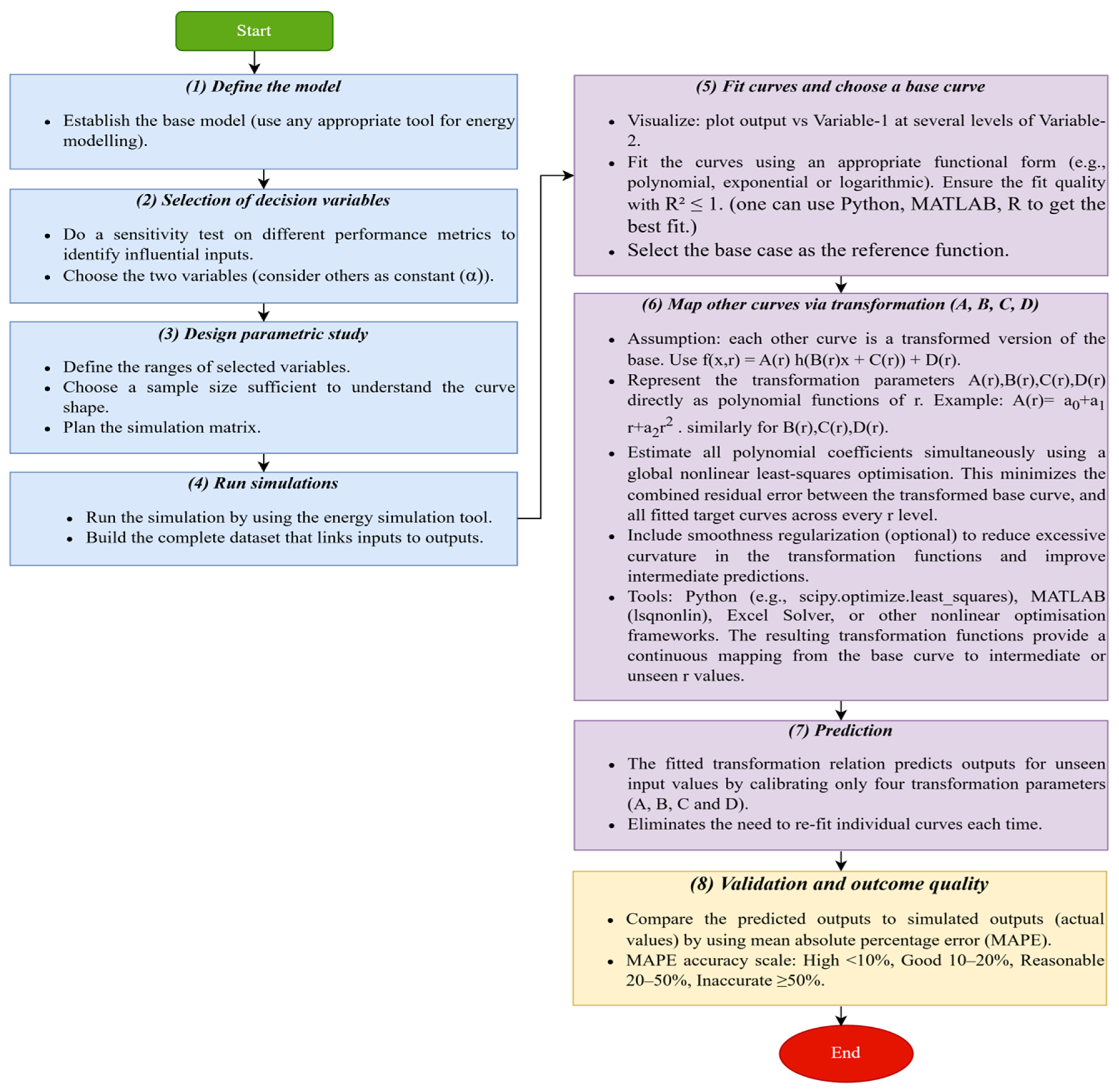
• Establishment of Base Model: At first, it is necessary to establish a base model/case study in a building energy modeling environment (the procedure of establishing our base cases has been discussed in Section 3.1).
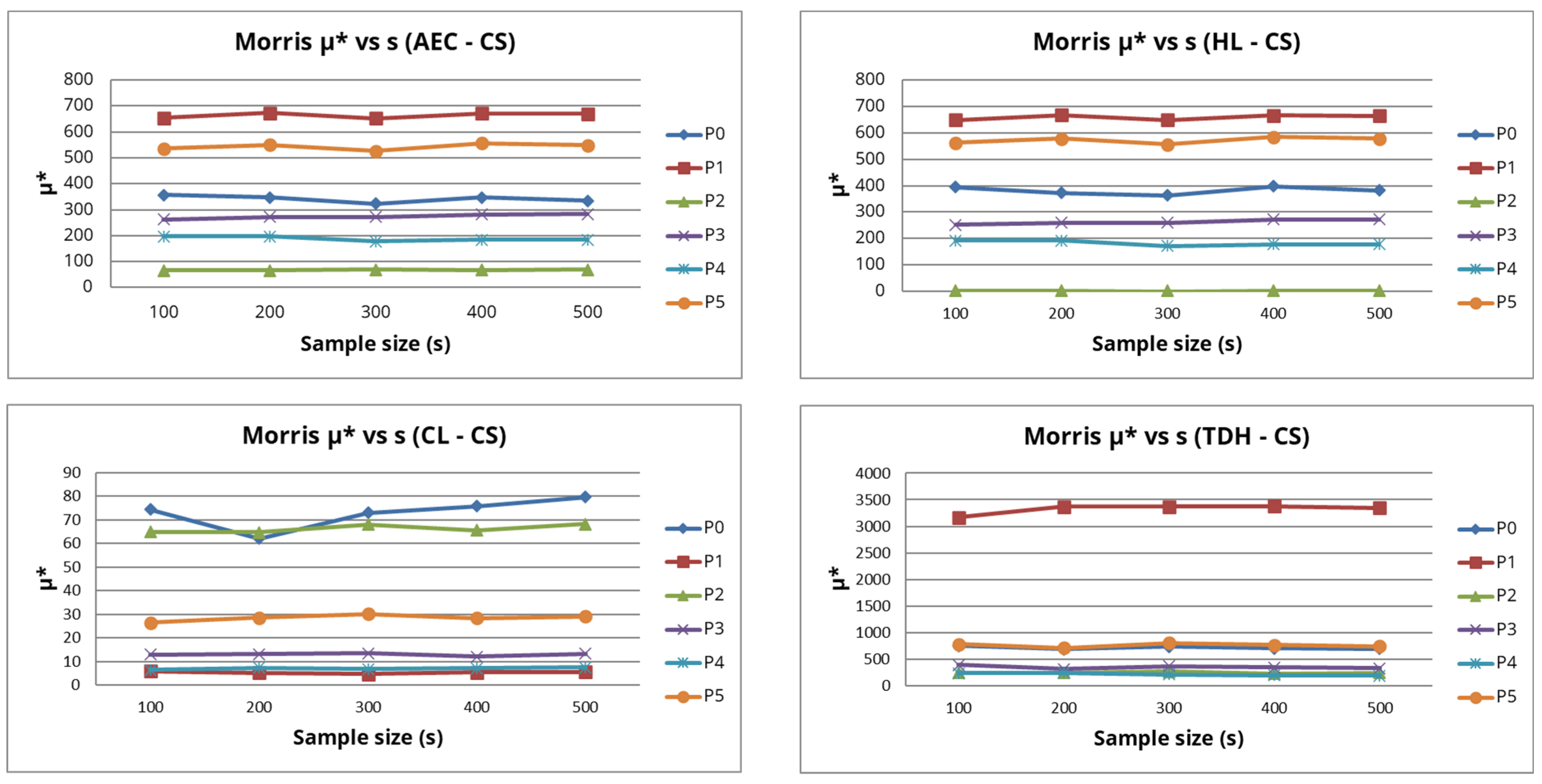
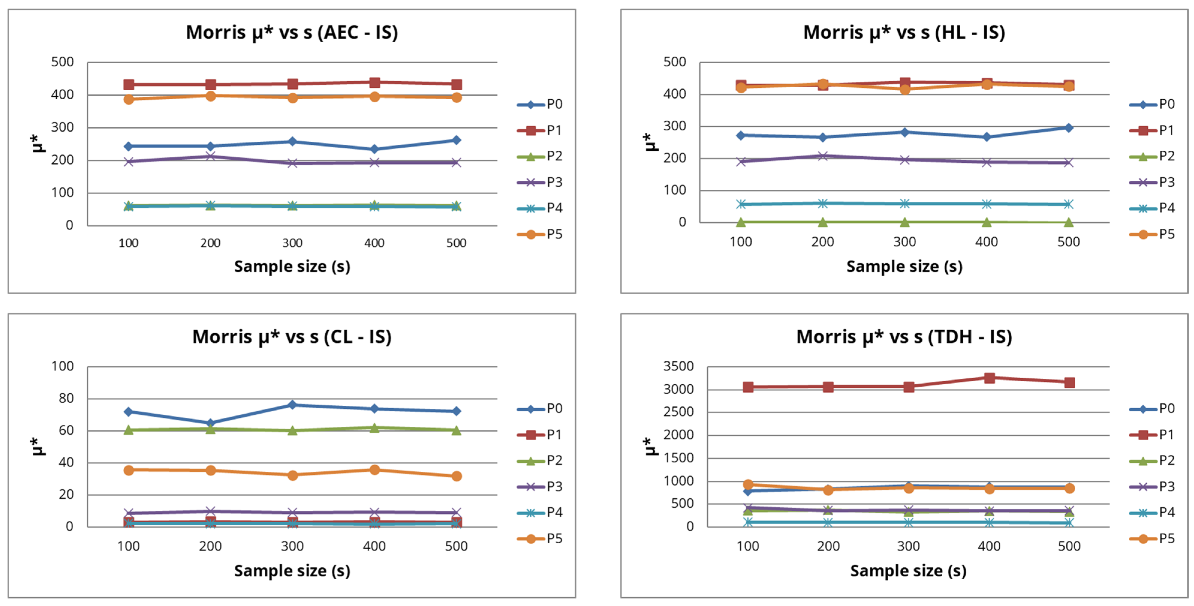
• Selection of Decision Variables: Instead of choosing the decision variables arbitrarily, a sensitivity analysis is needed to evaluate the influence of the input parameters on different performance metrics. After that, the two most influential parameters can be selected for analysis on the chosen performance metrics, such as AEC, HL, CL and TDH.
• Design the Parametric Study: In this step, the ranges of the two selected input variables were defined. The sample size was chosen to adequately capture the shape of the curve. A total of 16 unique input combinations (4 values of length × 4 values of aspect ratio) were considered for each orientation, resulting in 128 samples across all eight orientations. Mathematically, the rationale is that the number of points must meet or exceed the number of independent parameters in the function’s formula [60]. Moreover, at least four points are recommended per curve to understand the shape of the curve [61].
• Run Simulations: After the preparation of the sample size, the parametric cases were simulated with the help of an energy simulation tool called jEPlus. Therefore, a complete dataset was established that links inputs to outputs.
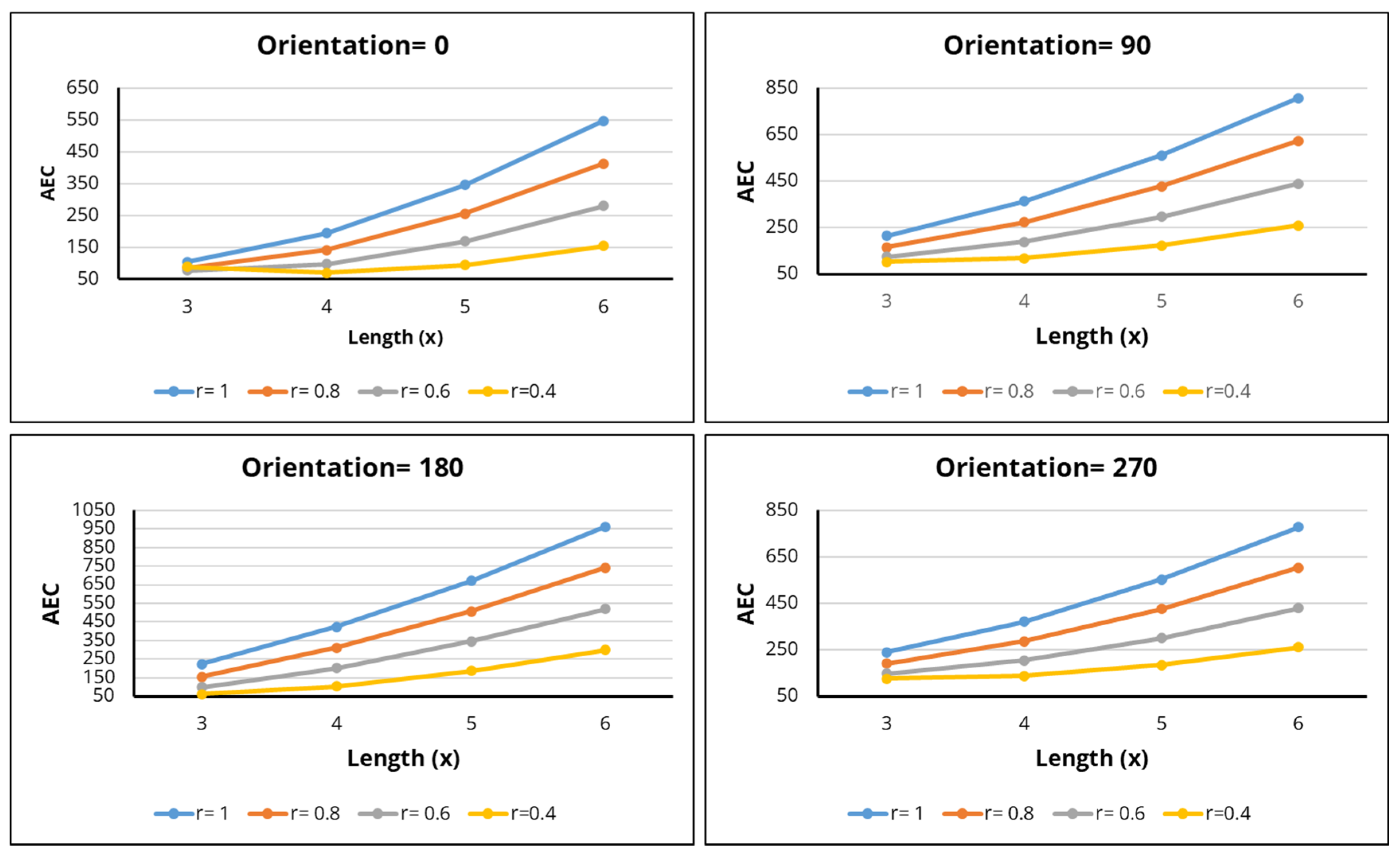
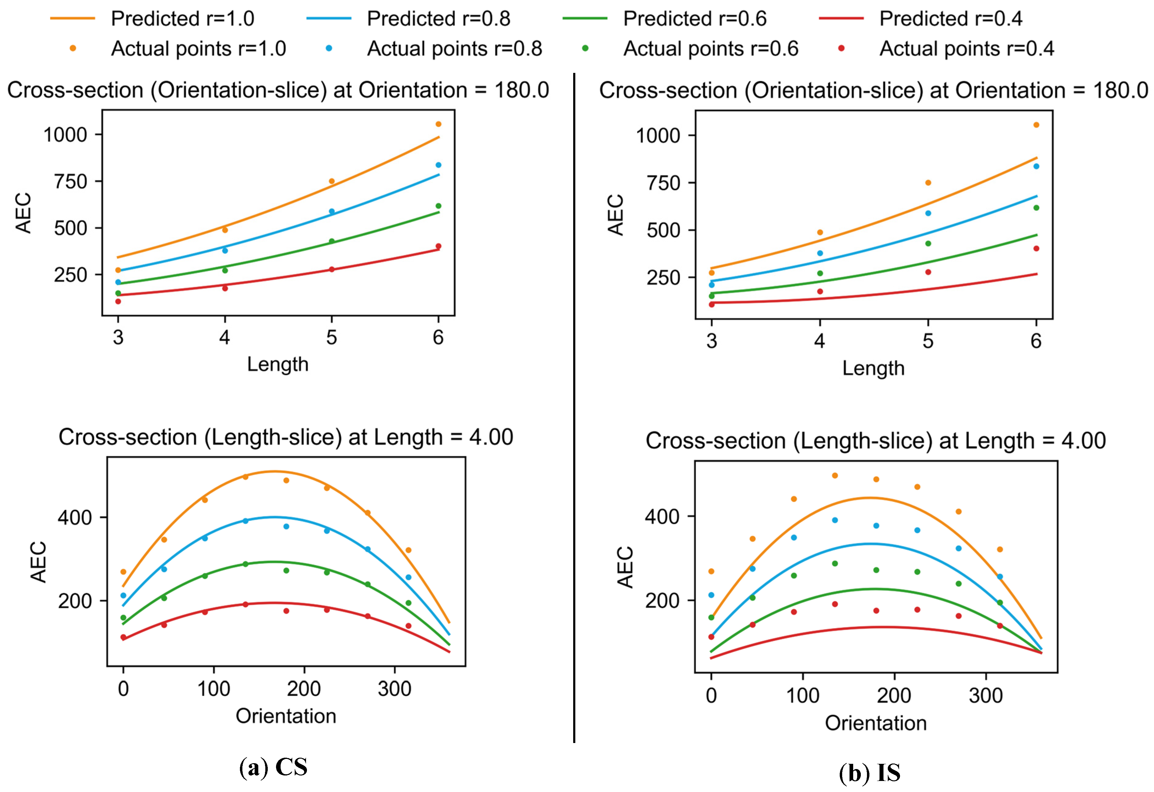
• Fit the Curves and Choose a Base Function: At this stage, graphs were plotted by using the dataset to visualize the output trends, with one variable examined across the levels of the other. Each curve was fitted using an appropriate functional form (e.g., polynomial, exponential, or logarithmic). Among these, a quadratic polynomial h(x) = ax² + bx + c provided the best fit across all curves. A satisfactory fit quality was ensured, with R² values close to 1 for the fitted quadratic curves. From these fitted curves, a base case (r = 1) was selected as the reference function. A Python (v3.13.5)routine was used to derive the best fit in this study, but any equivalent mathematical environment can also be used.
• Transformation of Other Curves: The idea was to represent each target curve as a transformed version of the selected base curve. Therefore, the transformation equation was defined as $\mathrm{f}\left(\mathrm{\alpha },\mathrm{r},\mathrm{x}\right)=\mathrm{A}\left(\mathrm{r}\right)\left[\mathrm{h}\left(\mathrm{B}\left(\mathrm{r}\right).\mathrm{x}+\mathrm{C}\left(\mathrm{r}\right)\right)\right]+\mathrm{D}\left(\mathrm{r}\right)$, where h(x) = f(α, 1, x) is the base function for r = 1. Here, α represents the fixed variable, while A(r), B(r), C(r) and D(r) are the transformation parameters. Specifically, A(r) controls vertical stretching/compression, B(r) controls horizontal stretching/compression, C(r) controls horizontal shifting, and D(r) controls the vertical shifting. Instead of estimating the transformation parameters separately for each (r) and then fitting them afterward, the coefficients of A(r), B(r), C(r), and D(r) were optimized simultaneously using a global nonlinear least-squares approach. In this formulation, each transformation function was represented as a quadratic function of r (ar² + br + c), and the optimization minimized the combined error between all transformed base curves and the corresponding fitted target curves within the selected fitting region. A smoothness regularization term was also included to reduce excessive curvature in the transformation functions and improve interpolation stability for intermediate (r) values.
• Prediction: Once fitted, the transformation relation allows the prediction of AEC for unseen input values. By calibrating only four transformation parameters, the need to re-fit individual curves each time was eliminated, making the approach generic and function-independent.
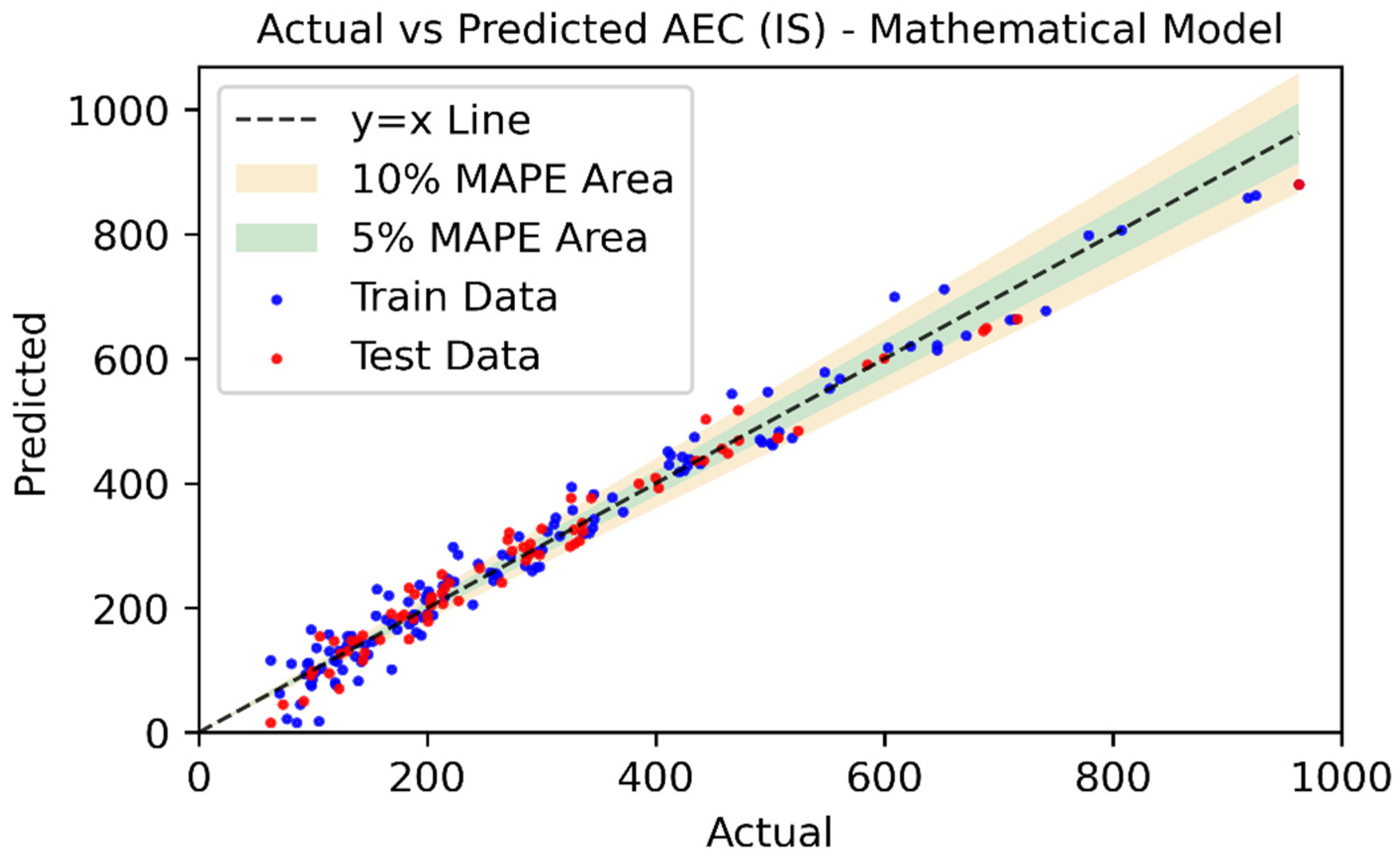
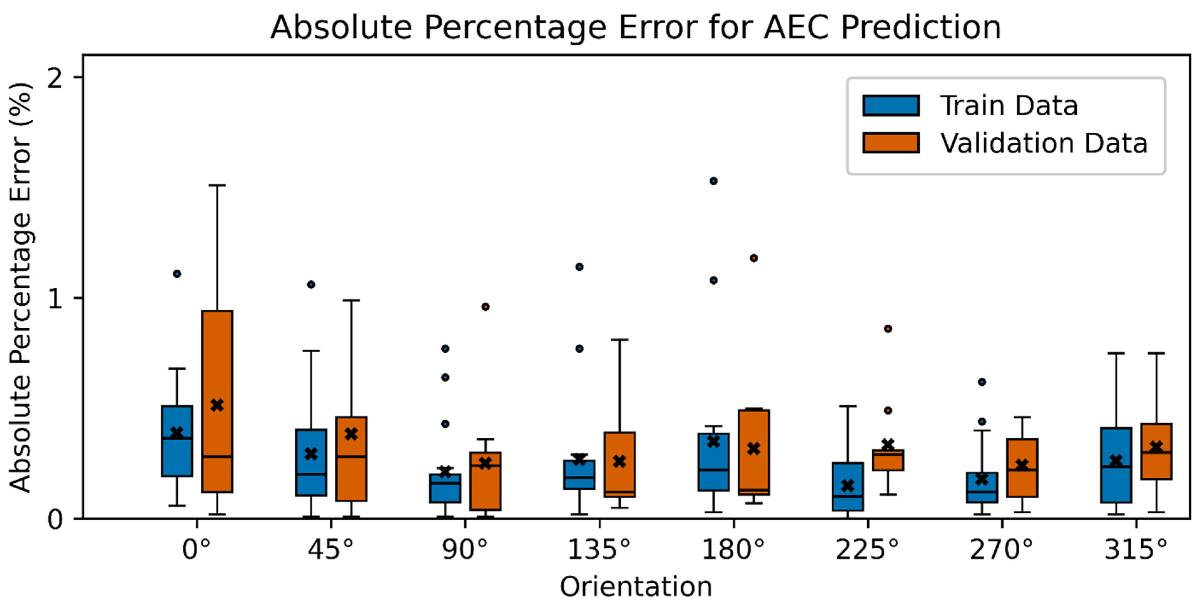
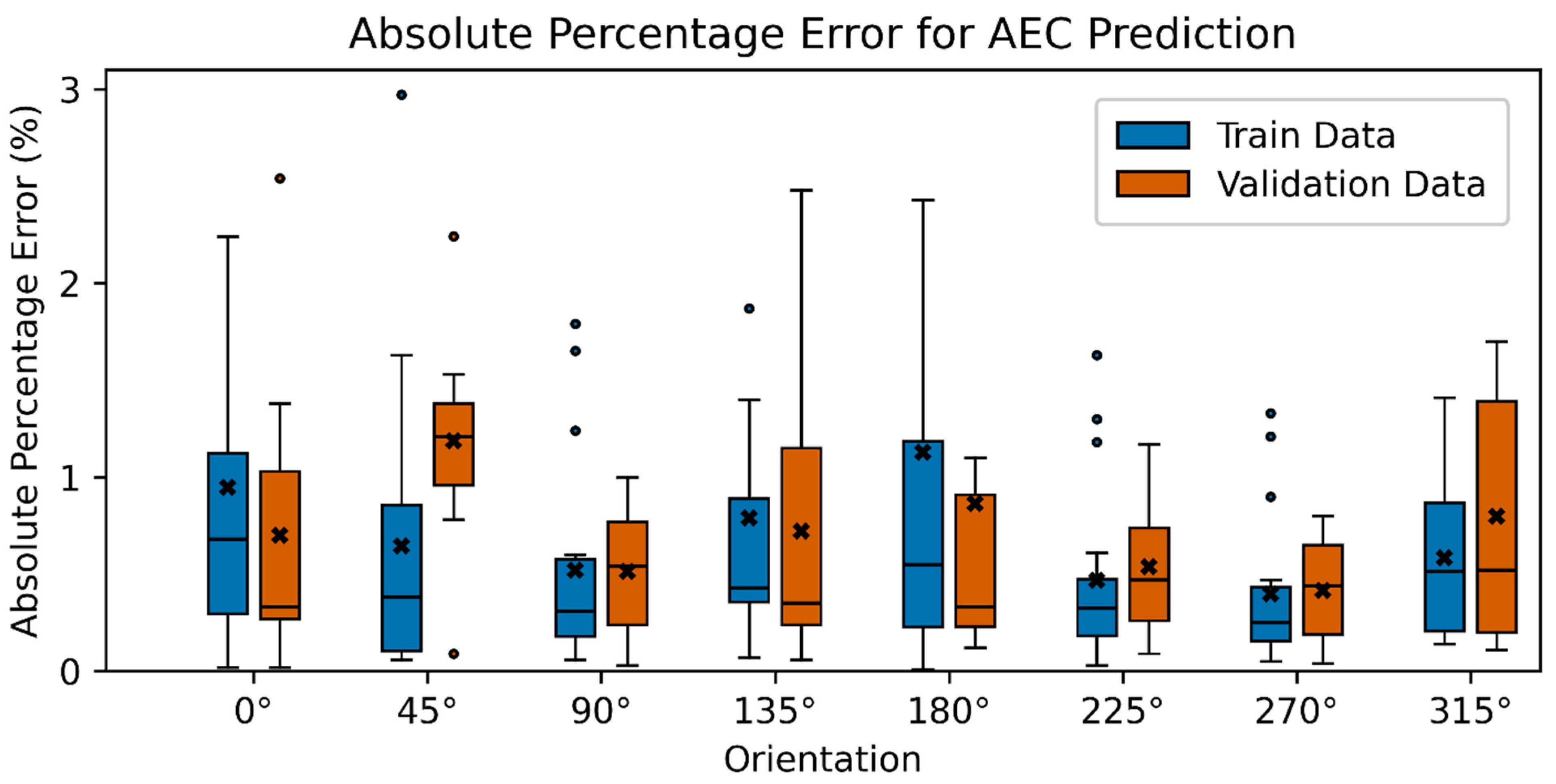
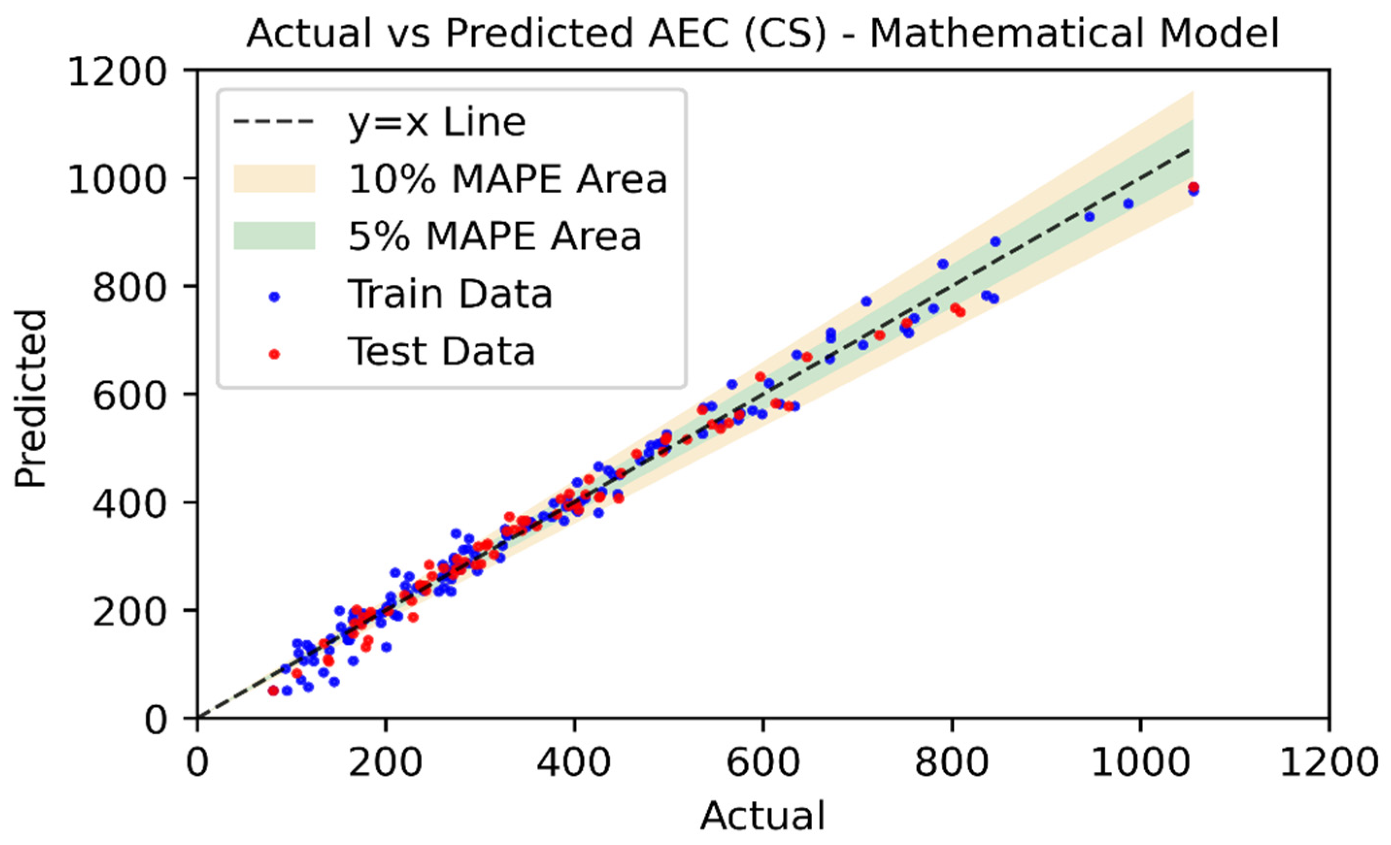
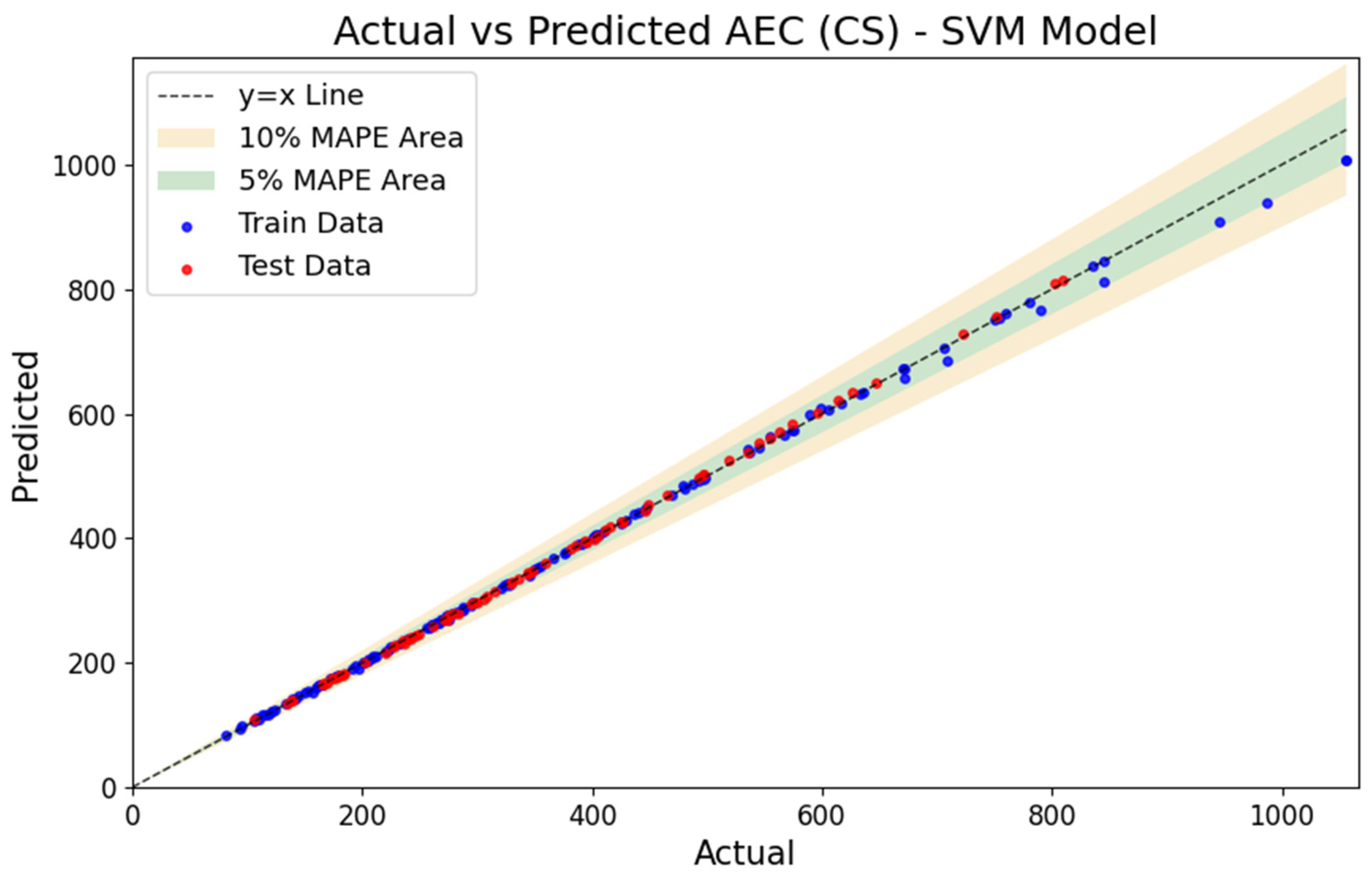
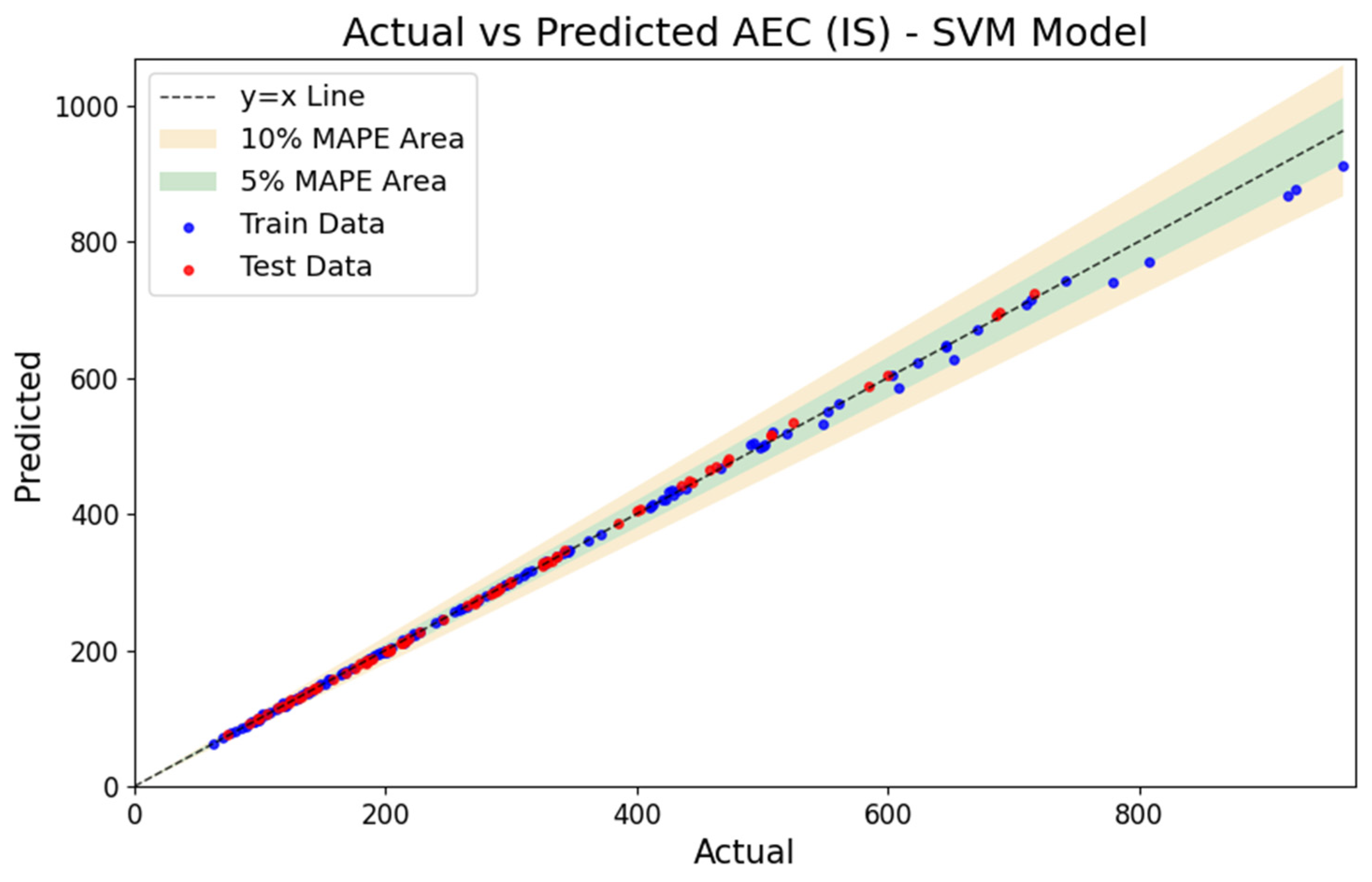
• Validation and Quality Classification: Model accuracy is assessed by comparing predicted and simulated values using MAPE,

  $$\mathrm{M}\mathrm{A}\mathrm{P}\mathrm{E}={\displaystyle \frac{1}{\mathrm{n}}}{\displaystyle \sum _{\mathrm{i}=1}^{\mathrm{n}}\frac{\left|{\mathrm{o}}_{\mathrm{i}}-{\mathrm{p}}_{\mathrm{i}}\right|}{{\mathrm{o}}_{\mathrm{i}}}}\times 100.$$

Here, n = sample size, o_i = observed (actual) value at the i-th data point and p_i = predicted value at the i-th data point. Nevertheless, Accuracy is categorized as high if MAPE < 10%, good if 10% < MAPE < 20%, reasonable if 20% < MAPE < 50%, and inaccurate if MAPE > 50% [62,63,64].

3.3.2. Stage 2 (Three-Variable Case)

As mentioned in Section 3.3.1, the two-variable approach has been extended to three variables by considering orientation (z) as a third input. With the inclusion of z, this is no longer a set of curves but becomes a surface in (z, x) for each r. The idea has been kept similar: consider a base surface at a specific r value, then express all the surfaces as the transformed version of this base case. The workflow has been summarized in Figure 5, where only steps 5–7 are presented, as steps 1–4 and 8 are unchanged from Figure 4. This workflow is also applicable to other building models with any chosen set of three variables. The procedure for developing steps 5–7 is discussed below.

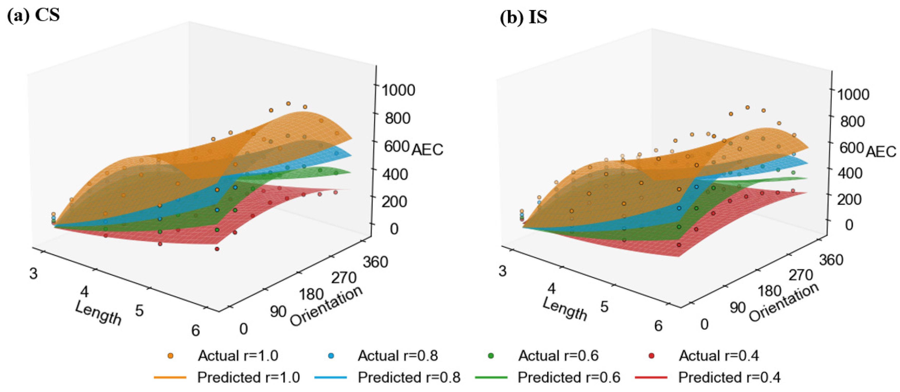
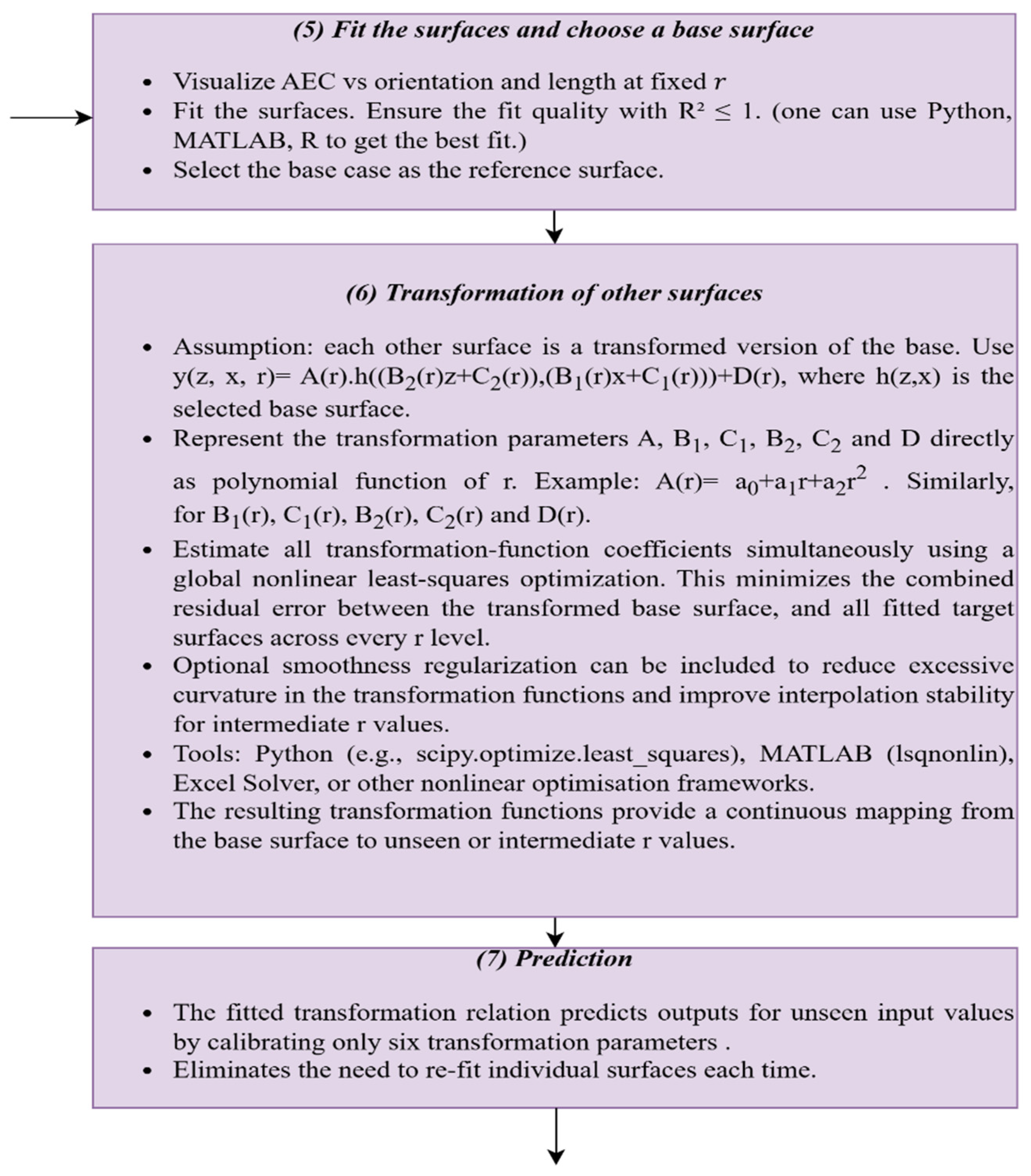
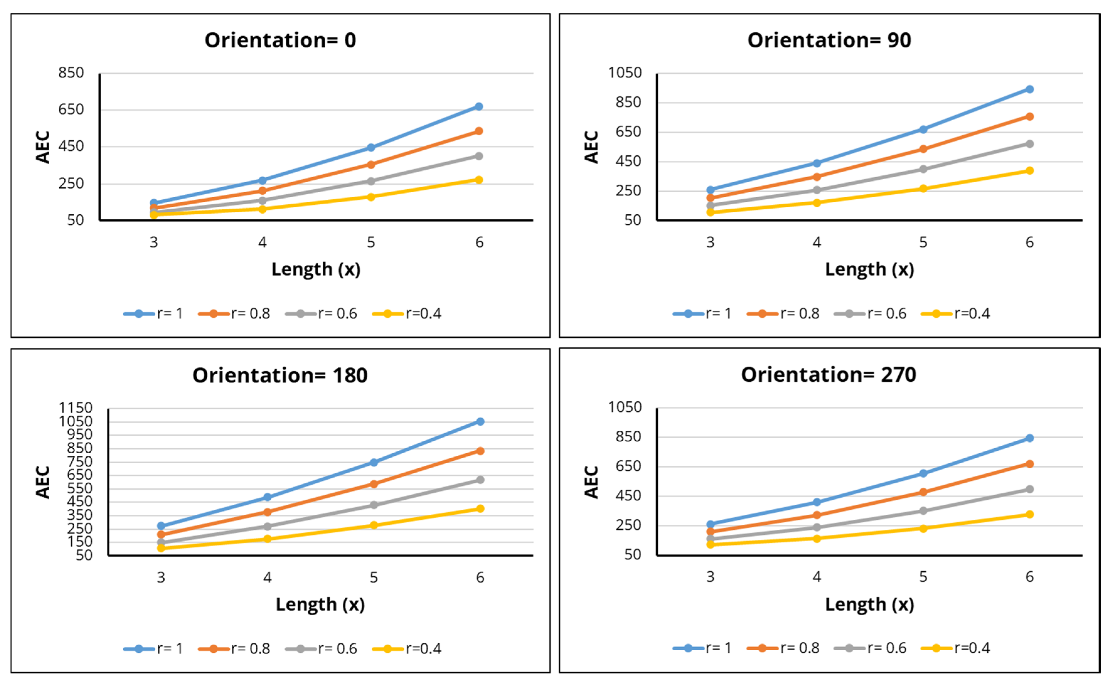
• Fit the Surfaces and Choose a Base Function: The outputs were visualized in three dimensions by plotting AEC as a function of orientation (z) and length (x) at a fixed aspect ratio (r). The quadratic surface $\mathrm{h}\left(\mathrm{z},\mathrm{x}\right)={\mathrm{a}}_0+{\mathrm{a}}_1\mathrm{z}+{\mathrm{a}}_2\mathrm{x}+{\mathrm{a}}_3{\mathrm{z}}^2+{\mathrm{a}}_4\mathrm{z}\mathrm{x}+{\mathrm{a}}_5{\mathrm{x}}^2$ provided the best fit for all the surfaces with R² = 0.98. This is the simplest polynomial that can effectively represent curvature in both directions and their interrelation. Moreover, r = 1 was selected as the base surface among the surfaces.
• Transformation of Other Surfaces: The transformation function in this case was formulated as $\mathrm{y}\left(\mathrm{z},\mathrm{x},\mathrm{r}\right)=\mathrm{A}\left(\mathrm{r}\right)\cdot \mathrm{h}\left(\left({\mathrm{B}}_2\left(\mathrm{r}\right)\mathrm{z}+{\mathrm{C}}_2\left(\mathrm{r}\right)\right),\left({\mathrm{B}}_1\left(\mathrm{r}\right)\mathrm{x}+{\mathrm{C}}_1\left(\mathrm{r}\right)\right)\right)+\mathrm{D}\left(\mathrm{r}\right)$. Here, A and D depict vertical scaling and shifting. Moreover, B₁ and C₁ are horizontal scaling and shifting along the x axis, while B₂ and C₂ do the same along the z axis. Instead of estimating these transformation parameters separately for each (r) and then fitting them afterward, the coefficients of A(r), B₁(r), C₁(r), B₂(r), C₂(r), and D(r) were optimized simultaneously using a global nonlinear least-squares approach. Each transformation function was represented as a quadratic function of r (a₀ + a₁r + a₂r²), and the optimization minimized the combined error between all transformed base surfaces and the corresponding fitted target surfaces across the selected fitting region. A smoothness regularization term was also included to reduce excessive curvature in the transformation functions and improve interpolation stability for intermediate r values.
• Prediction: In this step, the transformation relation predicts the AEC for any unseen combination of orientation, length and aspect ratio. Therefore, calibrating six transformation parameters (A, B₁, C₁, B₂, C₂ and D) eliminates the need to re-fit individual surfaces, making the workflow generic and computationally efficient.

As the next step, the same three-variable dataset was also examined using an ML approach. The motivation for introducing ML is that purely mathematical curve or surface fitting assumes a predetermined functional form (e.g., quadratic), which may not fully capture nonlinear or interaction effects among multiple variables. In contrast, ML models can learn complex and nonlinear relationships directly from data without requiring an explicit equation. However, this flexibility comes at the cost of interpretability and the need for a sufficiently large and well-distributed dataset to avoid overfitting.

For this stage, the SVM with a radial basis function (RBF) kernel was adopted, as it has been consistently demonstrated to achieve high accuracy and stability in building energy prediction tasks involving limited datasets and nonlinear relationships [22]. The RBF kernel provides strong generalization by mapping input variables into an infinite-dimensional feature space through localized Gaussian functions, enabling the model to represent nonlinear variations in energy performance that cannot be easily captured by polynomial functions. In this analysis, 128 samples were used for training, and 72 independent simulation samples were used for testing within the same predefined parameter space. A fixed random seed of 42 was used to ensure reproducibility.

The SVM model was implemented within a pipeline structure to ensure a reproducible and standardized workflow. First, the input features were normalized using a StandardScaler to eliminate the effect of variable magnitude differences. The regression model with the RBF kernel was then trained within a grid-search cross-validation framework to identify the optimal hyperparameters. The search space included penalty parameter C (1, 10, 100, 1000), kernel width (0.1, 0.01, 0.001), and ε-insensitive loss margin (0.1, 0.5, 1.0, 2.0), while model performance was evaluated using repeated k-fold cross-validation (5 splits × 5 repeats) to ensure statistical reliability. The optimal configuration was determined by minimizing the mean absolute error (MAE), and the final trained model was subsequently used to predict the annual energy consumption (AEC) for unseen data.

This approach enables a data-driven and flexible predictive framework that complements the earlier mathematical fitting by effectively capturing nonlinear relationships between building geometry and energy performance.

3.3.3. Stage 3 (Multi-Variable Case)

In the final stage, the predictive modeling framework was extended to a comprehensive multi-variable (more than 3) analysis by training and evaluating four ML models such as artificial neural network (ANN), support vector machine (SVM), random forest (RF) and decision tree (DT). These four ML models were selected from the available ML algorithms because they are frequently used in building energy prediction studies [65]. Also, these models provide a balanced comparison of kernel-based, neural network, ensemble and tree-based modeling approaches. The objective of this stage was to establish a robust comparative framework for predicting the four key energy performance indicators: AEC, HL, CL, and TDH, using the decision variables/retrofit options listed in Table 5.

To capture variability in sample size and assess model stability, LHS [66] was employed to generate five distinct datasets containing 100, 200, 300, 400, and 500 samples, respectively. Each dataset was created separately for both the CS and IS base models, resulting in ten unique data groups. This design enabled systematic evaluation of model performance as a function of data size and spatial configuration.

For each dataset, all four ML algorithms were trained independently for the four output variables (AEC, HL, CL, and TDH). Prior to model training, input features were standardized using a StandardScaler to ensure uniform scaling and improve numerical stability. Model training and hyperparameter optimization were conducted within a grid search cross-validation framework, using a repeated k-fold cross-validation strategy to ensure statistical robustness and mitigate overfitting. The performance of the above-mentioned four ML models was evaluated using R², mean absolute error (MAE), and root mean square error (RMSE).

I. ANN: A feed-forward neural network was implemented using three hidden layers (64-128-64 neurons) with ReLU activation functions and dropout regularization (0.2) to prevent overfitting. The network was trained using the Adam optimizer and mean squared error loss function with an early-stopping criterion (patience = 50) based on validation loss.

II. SVM: The SVM regression model employed an RBF kernel, with hyperparameter tuning over penalty parameter C (1, 10, 100, 1000), ε-insensitive loss margin (0.1, 0.5, 1.0, 2.0), and kernel width γ (scale, 0.1, 0.01, 0.001). A 5-fold × 5-repeat cross-validation setup ensured consistent evaluation across datasets.

III. RF: The ensemble RF model used 100, 200, 500 estimators with varied tree depths (None, 10, 20, 30) and node-splitting parameters (min_samples_split = 2, 5, 10, min_samples_leaf = 1, 2, 4). The max_features parameter was also tuned to [sqrt, log2, None]. Repeated 5 × 3 cross-validation was applied to balance bias and variance trade-offs.

IV. DT: A standalone decision-tree regressor was trained using multiple split criteria (squared_error, friedman_mse, absolute_error) and depths (5, 10, 20, 30). Additional parameters, including min_samples_split (2, 5, 10), min_samples_leaf (1, 2, 4), and max_features (None, sqrt, log2), were optimized using the same repeated 5 × 3 cross-validation.

For all Stage 3 ML models, an 80:20 train–test split with a fixed random seed of 42 was used. Each output variable was trained separately. The training time and final hyperparameters were recorded for each model, sample size, and space type to support the comparison in Section 4.6. The final tuned models for each configuration (space type × sample size × algorithm × output) were stored for subsequent performance analysis. This structured approach allows for a quantitative comparison of model accuracy, convergence behavior, and scalability across different data resolutions and spatial boundary conditions, thereby providing a generalized and reproducible methodology for multi-variable energy-performance prediction in residential retrofits.

4. Results and Discussions

4.1. Two-Variable Analysis: Patterns and Fitting

As mentioned in Section 3.3.1, after establishing the complete dataset, it is necessary to plot the graphs and examine the resulting curve patterns to establish the required mathematical relationships.

For the CS model, Figure 6 presents AEC against the length x across different r values at 0°, 90°, 180°, and 270°. It has been observed that AEC increased with increasing values of x and r, respectively. The highest AEC occurred at r = 1, while the lowest was at r = 0.4. However, the magnitude of AEC varied with orientation, while the shape of the curve family remained consistent. The curves for different r did not cross, and their spacing changed gradually with x. Therefore, r = 1 was considered as the base case for subsequent curve fitting and transformation due to the curves’ consistent behavior. Moreover, Figure 7 exhibits the IS model for the same four orientations, and the qualitative behavior matched the CS. The family of the curves remained orderly and well separated, and thus r = 1 was also taken as the base for the IS model as well. However, the remaining four orientations (45°, 135°, 225°, 315°) display the same qualitative pattern for both CS and IS and are provided in the Supplementary Materials (Figures S1 and S2). Therefore, these results provide the foundation for the curve-fitting method introduced next.

As stated in step 6 of Section 3.3.1, the other three curves are considered as the transformed version of the base case r = 1, using the transformation equation f = A(r)[h(B(r)x + C(r))] + D(r). For each orientation, this yields five equations (one base fit plus four transformations), totaling forty equations across eight orientations. These five equations enable AEC prediction for a given orientation.

For example, in case of the CS model, at orientation 0°, for r = 1, the best fit equation with R² = 1 was obtained as

$$\mathrm{h}\left(\mathrm{x}\right)=25.185{\mathrm{x}}^2-50.899\mathrm{x}+70.788$$

(4)

The transformation parameters A, B, C and D were then represented as quadratic functions of r, which provided the best fit. The resulting equations are

$$\mathrm{A}(\mathrm{r})=-0.15794{\mathrm{r}}^2+0.625057\mathrm{r}+0.54445$$

(5)

$$\mathrm{B}(\mathrm{r})=-0.03633{\mathrm{r}}^2+0.238807\mathrm{r}+0.79165$$

(6)

$$\mathrm{C}(\mathrm{r})=-1.60911{\mathrm{r}}^2+4.041759\mathrm{r}-2.42889$$

(7)

$$\mathrm{D}(\mathrm{r})=14.10948{\mathrm{r}}^2-86.4375\mathrm{r}+71.83398$$

(8)

Therefore, the predicted AEC at any (x, r) is obtained by substituting A(r), B(r), C(r) and D(r) from Equations (5)–(8) into the transformation f = A(r)[h(B(r)x + C(r))] + D(r) and computing h(B(r)x + C(r)) using the base function in (4). The same procedure is applied to all other orientations. Moreover, the IS model also followed the same transformation framework. In a similar manner, at 0°, the IS model’s best-fit equation for r = 1 was attained with R² = 1 as

$$\mathrm{h}\left(\mathrm{x}\right)=22.665{\mathrm{x}}^2+42.949\mathrm{x}-110.618$$

(9)

The IS model utilized the same quadratic formulation in r as the CS model, and the equations are

$$\mathrm{A}\left(\mathrm{r}\right)=2.667417{\mathrm{r}}^2-3.49423\mathrm{r}+1.790844$$

(10)

$$\mathrm{B}(\mathrm{r})=-1.43742{\mathrm{r}}^2+2.108894\mathrm{r}+0.357144$$

(11)

$$\mathrm{C}(\mathrm{r})=-7.99594{\mathrm{r}}^2+16.58949\mathrm{r}-8.58462$$

(12)

$$\mathrm{D}(\mathrm{r})=404.0972{\mathrm{r}}^2-845.218\mathrm{r}+434.8422$$

(13)

The IS case followed the same transformation procedure as CS, with its own base curve, and fitted A(r), B(r), C(r), D(r) to predict AEC across (x, r) and orientations.

4.2. Prediction Accuracy and Agreement Across Orientations (Two-Variable Case)

After completing the above steps, graphs comparing simulation (actual) outputs with model predictions were produced to assess agreement. The results for both CS and IS are depicted in Figure 8 and Figure 9. For both models, all 128 combinations were evaluated on a grid defined by x = {3, 4, 5, 6}, r = {0.4, 0.6, 0.8, 1.0} and z = 0° to 315° with 45° steps. Moreover, to test the generalization beyond these selected points, unseen intermediate combinations such as x = {3.5, 4.5, 5.5} and r = {0.5, 0.7 and 0.9} were introduced at the same orientations, and we repeated the comparison. This served as an extra-point validation step.

Figure 8 shows the absolute percentage error of different orientations for the CS model. The blue and orange color box plots represent variation in the absolute error percentage of the training and validation data based on different orientations. Here, data used to fit the mathematical model is considered as the training data. Plots show a similar variation for training and validation data, confirming that mathematical equations are not overfitted and have an error less than 1%.

For the eight orientations, the MAPE accuracy of the training set was achieved as 0.38%, 0.29%, 0.21%, 0.26%, 0.35%, 0.15%, 0.18%, and 0.26%, respectively, which falls in the high-accuracy category (MAPE < 10%). Moreover, the MAPE values remained within the high-accuracy band (MAPE < 10%) for both training and validation cases. For the validation case, the MAPE values are 0.51%, 0.38%, 0.25%, 0.26%, 0.32%, 0.34%, 0.24%, and 0.32%, respectively.

Following the CS results, the IS model demonstrated the same qualitative agreement, with the MAPE accuracy less than 10% (Figure 9). Orientation-wise MAPE for the 128 training points spans 0.40–1.13% (median 0.62%), and for the validation points spans 0.42–1.19% (median 0.71%), indicating high accuracy.

The above results clearly demonstrate that a straightforward analytical relation can be highly effective for rapid performance assessment when retrofit decisions focus on one or two variables. Although this type of analytical relation was developed in this study, their high accuracy can be interpreted in relation to commonly used ML surrogate models in building energy prediction. The low MAPE values of this two-variable analytical relation can achieve high accuracy comparable to data-driven models with better interpretability and lower computational complexity. This agrees with recent studies showing that simple analytical models can achieve useful accuracy while being easier to interpret and less computationally demanding than complex ML models [67,68]. Moreover, the approach is particularly valuable in residential retrofits, where budget constraints typically limit decision-makers to select a small number of retrofit measures.

4.3. Three-Variable Analysis: Patterns and Fitting

After assembling the full (z, x, r) dataset, the 3D surfaces were inspected for both CS and IS models (Figure 10). Each surface plotted predicted AEC over orientation z and length x for several aspect-ratio levels r along with the actual data points. It was observed that AEC escalated smoothly with x, while variations in z primarily shift the overall level without abrupt changes. For any (x, z), the layers of r remained well-ordered, with r = 1 the highest and r = 0.4 the lowest, and the surfaces did not cross.

These patterns justify adopting a single base surface at r = 1 and expressing the remaining r levels as the transformed version of the base surface. According to Section 3.3.2, the transformation equation for this case has been formulated as

$$\mathrm{y}\left(\mathrm{z},\mathrm{x},\mathrm{r}\right)=\mathrm{A}\left(\mathrm{r}\right)\cdot \mathrm{h}\left(\left({\mathrm{B}}_2\left(\mathrm{r}\right)\mathrm{z}+{\mathrm{C}}_2\left(\mathrm{r}\right)\right),\left({\mathrm{B}}_1\left(\mathrm{r}\right)\mathrm{x}+{\mathrm{C}}_1\left(\mathrm{r}\right)\right)\right)+\mathrm{D}\left(\mathrm{r}\right)$$

(14)

Now, the following quadratic surfaces were obtained as the best fit at r = 1 for the CS and IS models respectively.

$$\mathrm{h}(\mathrm{z}, \mathrm{x})=-155.688+3.313\mathrm{z}+3.325\mathrm{x}-0.01{\mathrm{z}}^2-0.009\mathrm{z}\mathrm{x}+23.661{\mathrm{x}}^2$$

(15)

$$\mathrm{h}(\mathrm{z}, \mathrm{x})=-93.035+3.16\mathrm{z}-37.446\mathrm{x}-0.01{\mathrm{z}}^2+0.04\mathrm{z}\mathrm{x}+24.91{\mathrm{x}}^2$$

(16)

Moreover, the transformation parameters A, B₁, B₂, C₁, C₂ and D were fitted as the quadratic function of r that provided the best fit and also consistent with the cross-section of the surface in either direction (orientation-slice or length-slice) (see Figure 11).

Therefore, the equations for the transformation parameters for the CS and IS models are depicted in Equations (17) and (18) as

$$\left.\begin{array}{l}\mathrm{A}(\mathrm{r})=-0.159+1.964\mathrm{r}-0.83{\mathrm{r}}^2\\ {\mathrm{B}}_1\left(\mathrm{r}\right)=1.515-1.376\mathrm{r}+0.879{\mathrm{r}}^2\\ {\mathrm{C}}_1\left(\mathrm{r}\right)=-4.571+9.006\mathrm{r}-4.459{\mathrm{r}}^2\\ {\mathrm{C}}_2\left(\mathrm{r}\right)=29.625+5.335\mathrm{r}-36.238{\mathrm{r}}^2\\ \mathrm{D}\left(\mathrm{r}\right)=148.11-303.225\mathrm{r}+155.414{\mathrm{r}}^2\end{array}\right\}$$

(17)

$$\left.\begin{array}{l}\mathrm{A}(\mathrm{r})=-1.02+4.52\mathrm{r}-2.492{\mathrm{r}}^2\\ {\mathrm{B}}_1\left(\mathrm{r}\right)=2.547-4.027\mathrm{r}+2.484{\mathrm{r}}^2\\ {\mathrm{C}}_1\left(\mathrm{r}\right)=-10.488+21.916\mathrm{r}-11.47{\mathrm{r}}^2\\ {\mathrm{C}}_2\left(\mathrm{r}\right)=29.625+5.335\mathrm{r}-36.238{\mathrm{r}}^2\\ \mathrm{D}\left(\mathrm{r}\right)=189.244-405.393\mathrm{r}+217.212{\mathrm{r}}^2\end{array}\right\}$$

(18)

Now, the values of A, B₁, B₂, C₁, C₂, and D are obtained from Equation (17) for CS and Equation (18) for IS, and they are substituted into Equation (14). However, in Equation (14), the term h is computed using the base function in Equation (15) for CS and Equation (16) for IS. This process enables the prediction of the AEC at any given (z, x, r).

4.4. Prediction Accuracy and Agreement in Three-Variable Case

In the three-variable case, the predictive performance of the mathematical models developed for the CS and IS categories (Figure 12 and Figure 13) was evaluated using scatter plots of actual AEC versus predicted AEC. The plots include both the training samples (x = {3, 4, 5, 6}, r = {0.4, 0.6, 0.8, 1.0}, z = 0° to 315° in 45° steps) and the test samples (x = {3.5, 4.5, 5.5}, r = {0.5, 0.7, 0.9}), together with the 5% and 10% MAPE envelopes, providing a visual reference for the expected accuracy range.

Across both CS and IS scenarios, the predicted values align closely with the y = x reference line, reflecting strong agreement between predicted and actual AEC values. The majority of the points fall within the 10% MAPE band, and a considerable proportion also lie within the more stricter 5% band, indicating that the models capture the main relationships among x, r, and z with good fidelity. The overlap between training and test distributions further suggests that the models generalize well to unseen parameter combinations. The error metrics reinforce this visual interpretation. For the CS model, the MAPE values were 8.38% for the training set and 5.82% for the extra-validation set. For the IS model, MAPE was 13.37% for the training set and 9.33% for the extra-validation set.

According to conventional thresholds, where MAPE < 10% indicates high accuracy and 10–20% indicates good accuracy, the CS model demonstrates high accuracy across both datasets. The IS model shows good accuracy for the training set and high accuracy for the extra-validation set.

Beyond overall accuracy, several critical observations emerge from the scatter distributions. A noticeable widening of the prediction scatter occurs at higher AEC values, particularly in the IS case. This indicates a mild proportional error effect, where prediction deviations increase with magnitude. Despite this, the majority of the points remain contained within the 10% envelope, suggesting that this proportionality does not undermine the overall reliability of predictions.

At lower AEC values, some points fall outside the preferred MAPE region. This is likely due to the narrowing of the MAPE tolerance bands at small magnitudes rather than an actual deterioration in model performance. Because MAPE is a relative metric, even small absolute differences can appear as large percentage errors when the denominator (actual AEC) is small.

Importantly, no systematic bias is evident in either model. The scatter does not preferentially shift above or below the y = x line, indicating that the mathematical formulation does not exhibit consistent over-prediction or under-prediction across the parameter space. This absence of directional bias, combined with the contained error-spread and strong clustering around the diagonal, demonstrates that the models achieve stable and balanced prediction behavior across both CS and IS configurations.

4.5. Prediction Accuracy and Agreement in Three-Variable Case Using Support Vector Machine (SVM)

Following the analytical modeling, the SVM with the RBF kernel was trained on the same three-variable dataset to evaluate its predictive performance for the AEC in both CS and IS configurations. The resulting scatter plots of actual versus predicted AEC (Figure 14 and Figure 15) again include the full training and test set, overlaid with 5% and 10% MAPE envelopes for consistent comparison.

Across both cases, the SVM predictions demonstrate a remarkably close alignment around the y = x reference line. Almost all data points in both training and test sets fall within the 5% MAPE band, indicating a remarkably high degree of predictive agreement. The overlap between training and test points further suggests that the SVM generalizes smoothly across previously unseen geometric and directional combinations.

Quantitatively, a direct comparison with the mathematical transformation approach further emphasizes the advantage of the SVM approach. For the CS model, the SVM achieved an average MAPE of 0.75% (min 0.01%, max 4.85%), compared with 8.04% (min 0.02%, max 54.51%) from the mathematical fitting. Similarly, for the IS, the SVM model yielded an average error of 0.91% (min 0.01%, max 5.47%), while the analytical model produced 18.47% (min 0.04%, max 626.73%). In addition to the reduced average error, the SVM also substantially limits extreme deviations, indicating much lower variance and far better stability across all parameter combinations.

Overall, the SVM model demonstrated superior predictive precision and robustness for the three-variable case, effectively reproducing the physical trends represented in the EnergyPlus simulations. While the analytical formulation offers interpretability and a closed-form mathematical structure, the SVM provides greater flexibility, scalability, and numerical accuracy, making it a more practical solution for complex multi-variable prediction tasks in retrofit energy modeling. Recent studies also demonstrate that ML models like SVM can achieve high accuracy while remaining much faster for complex multi-variable prediction tasks in retrofit energy modeling [69,70].

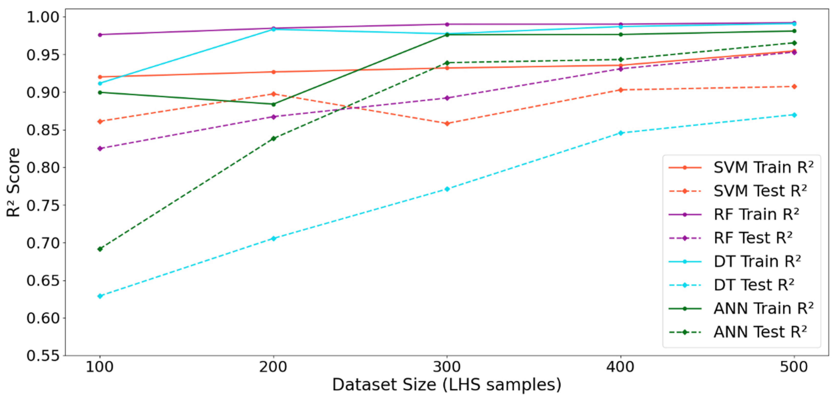
4.6. Prediction Accuracy and Agreement in Multi-Variable Case with ANN, SVM, RF, and DT

Figure 16 and Figure 17 represent the comparison of mean R² values for both training and testing splits of four ML models (ANN, SVM, RF, DT) across dataset sizes of 100, 200, 300, 400, and 500 samples for the CS and IS, respectively. All models demonstrated a clear positive correlation between dataset size and prediction accuracy, confirming that the learning process improved as the number of samples increased. In both figures, the overall pattern was consistent, and the R² values for training and testing splits progressively increased, while the gap between them narrowed, indicating better generalization and reduced overfitting with larger datasets.

Both RF and DT achieved the highest training R² across all dataset sizes, but their behavior differed substantially in generalization. RF showed a consistent improvement in testing R² with an increasing sample size, reaching around 0.95 for larger datasets. However, its training time was considerably higher than the other models, primarily due to the ensemble structure that builds multiple DTs and performs extensive averaging, leading to higher computational complexity.

In contrast, DT exhibited the lowest R² on the testing split, reflecting severe overfitting caused by its single-tree structure that partitions data greedily without ensemble averaging, making it highly sensitive to noise and small variations in the input space.

The SVM model maintained a consistent and narrow train–test gap in R², highlighting its robust generalization capability and strong performance even with limited data. The RBF kernel’s ability to model localized nonlinear relationships allowed SVM to perform reliably across all dataset sizes.

Meanwhile, the ANN displayed a continuous upward trend in both training and testing R² values, with the train–test gap diminishing as the dataset size increased. This behavior underscores the scalability and adaptability of the ANN. While the ANN requires more data to converge compared to SVM, its predictive accuracy and stability improve significantly once sufficient training samples are available.

Collectively, these results reaffirm that for multivariable cases (more than two variables), the proposed ML-based framework outperforms the analytical transformation approach discussed earlier in Stage 2. The machine learning models, particularly SVM and ANN, offer superior predictive accuracy, lower variance, and stronger scalability for multi-variable retrofit performance prediction. SVM is the most suitable choice when data availability is limited, while the ANN becomes the optimal model when larger and more diverse datasets are available, making the combined approach versatile and well-suited for complex building energy modeling tasks. The above findings are consistent with recent building energy prediction studies [71,72], where model performance has also been shown to depend on the data availability, variable complexity and prediction target. Therefore, the present framework provides not only predictive results but also actionable guidance for selecting a suitable surrogate according to data availability, computational effort, and problem complexity.

4.7. Cross-Climate Applicability of the Proposed Framework

After evaluating the staged predictive framework under the primary climate condition of Melbourne, the analysis was extended to seven additional climate conditions: Adelaide, Brisbane, Canberra, Darwin, Hobart, Perth and Sydney. The presented results were obtained by implementing the previously discussed predictive framework under these different climatic conditions. This analysis was conducted to examine whether the prediction trends observed in the primary case remained valid under various climatic scenarios.

Table 6. Cross-climate summary of Stage 1 (two-variable case) prediction accuracy.

Climate	Corner Space (CS) Train MAPE, Median (Range) (%)	Corner Space (CS) Extra-Validation MAPE, Median (Range) (%)	Intermediate Space (IS) Train MAPE, Median (Range) (%)	Intermediate Space (IS) Extra-Validation MAPE, Median (Range) (%)
Melbourne	0.27 (0.15–0.39)	0.32 (0.24–0.51)	0.62 (0.40–1.13)	0.71 (0.42–1.19)
Adelaide	0.20 (0.15–0.29)	0.25 (0.14–0.56)	0.36 (0.28–0.56)	0.35 (0.25–1.21)
Brisbane	0.12 (0.08–0.20)	0.15 (0.10–0.23)	0.16 (0.10–0.57)	0.15 (0.12–0.51)
Canberra	0.12 (0.09–0.22)	0.17 (0.12–0.35)	0.30 (0.20–0.63)	0.36 (0.22–0.77)
Darwin	0.04 (0.02–0.06)	0.09 (0.03–0.56)	0.05 (0.03–0.07)	0.83 (0.17–2.07)
Hobart	0.32 (0.27–0.52)	0.40 (0.24–0.69)	1.08 (0.63–1.18)	0.82 (0.50–1.15)
Perth	0.12 (0.04–0.19)	0.14 (0.06–0.20)	0.23 (0.15–0.39)	0.25 (0.10–0.45)
Sydney	0.13 (0.07–0.31)	0.19 (0.09–0.40)	0.33 (0.23–0.46)	0.29 (0.23–0.59)

Note: Median MAPE values and corresponding ranges were calculated from the eight analyzed orientations (0–315° at 45° intervals) for each climate and space type.

demonstrates that, across all climate conditions, the analytical method of Stage 1 maintained high prediction accuracy for both CS and IS. The indicated values were calculated from the eight analyzed orientations for each climate and space type. The values are expressed as the median MAPE with the corresponding ranges. For the CS model, the median train MAPE value remained between 0.04% and 0.40%, while the extra-validation median MAPE varied from 0.09% to 0.40%. Similarly, the train median MAPE ranged from 0.05% to 1.08% for the IS model, while the extra-validation median MAPE value stayed between 0.15% and 0.83%. It can be observed that for both CS and IS models, the MAPE values remained very low for different climate conditions, indicating that the two-variable analytical relation generalized well beyond the fitted points. Nevertheless, the corresponding errors for the IS model were slightly higher than the CS, suggesting that the IS case is more sensitive to climate variation. The results also highlight that higher IS error in Melbourne and Hobart may reflect the greater sensitivity of the analytical relation under heating-dominant conditions. However, the continued low errors in Perth, Brisbane and Darwin indicate that the same framework also remained stable for warmer climates where cooling demand dominates. Although different orientations and climates demonstrate some variability in the accuracy level, the analytical approach mentioned in Stage 1 remained robust and eventually provides a transferable pathway for various climatic conditions.

For both CS and IS,

Table 7. Cross-climate comparison of Stage 2 analytical (three-variable case) and support vector machine (SVM) accuracy.

Climate	(CS) A-Tr MAPE (%)	(CS) A-EV MAPE (%)	(CS) S-Tr MAPE (%)	(CS) S-EV MAPE (%)	(IS) A-Tr MAPE (%)	(IS) A-EV MAPE (%)	(IS) S-Tr MAPE (%)	(IS) S-EV MAPE (%)
Melbourne	8.38	5.82	0.75	0.77	13.37	9.33	0.89	0.94
Adelaide	9.56	7.75	0.27	0.63	14.94	12.72	0.94	0.81
Brisbane	9.15	8.67	0.31	0.45	15.54	15.57	0.36	0.51
Canberra	7.68	5.51	1.03	1.10	11.09	7.72	0.97	1.25
Darwin	6.72	6.74	0.27	0.38	10.20	10.57	0.31	1.75
Hobart	11.84	8.26	0.77	1.02	17.07	11.94	1.10	1.51
Perth	9.19	8.58	0.30	0.50	16.14	15.01	0.35	0.55
Sydney	11.51	10.02	0.25	0.62	16.91	14.80	0.39	0.73

Note: A = analytical, CS = corner space, EV = extra-validation, IS = intermediate space, S = SVM, Tr = train.

exhibited that SVM performed better compared to the three-variable analytical model across all climates. The analytical model provided acceptable outcomes for the CS and mostly remained in the range of high accuracy, while Sydney and Hobart moved to a good accuracy range. However, for IS, the analytical model was acceptable, but the error percentage is consistently higher compared to CS. The error percentage was affected by the climatic conditions, as the analytical model showed relatively better performance in Darwin, Canberra and Melbourne, but represented higher error in Sydney, Perth and Hobart. In contrast, SVM demonstrated very high accuracy, with lower MAPE values in every possible scenario, while the magnitude of SVM’s performance was affected by the climate. The improvement from the analytical model to SVM was more significant for IS than for CS, indicating that IS involves more intricate three-variable interactions.

Table 8. Cross-climate summary of best performing Stage 3 model for CS and IS.

Climate	Sample Sizes
	100		200		300		400		500
	CS	IS	CS	IS	CS	IS	CS	IS	CS	IS
Melbourne	SVM	SVM	SVM	SVM	ANN	ANN	RF	ANN/RF	ANN	ANN/RF
Adelaide	SVM	SVM	SVM	SVM	ANN	ANN/RF	ANN/RF	ANN/RF	ANN/RF	ANN/RF
Brisbane	SVM/RF	RF	SVM/RF	RF	ANN	RF	ANN/RF/SVM	RF	ANN/RF	ANN/RF
Canberra	SVM	SVM	SVM	SVM	ANN/RF/SVM	ANN/RF/SVM	RF/ SVM	ANN	ANN/RF/SVM	ANN/RF
Darwin	RF	RF	RF	SVM	RF/DT	RF/DT	RF *	RF *	RF *	RF *
Hobart	SVM	SVM	SVM	SVM	SVM/RF	ANN	RF	ANN/RF	ANN/RF	ANN/RF
Perth	SVM	RF	SVM	RF	ANN/RF/SVM	ANN/RF	ANN	ANN/RF	ANN	ANN/RF
Sydney	SVM	SVM	SVM	SVM	ANN/SVM	ANN	ANN/RF	ANN/RF/SVM	ANN/RF	ANN/RF

Note: Model selection is based on the highest average test R² across AEC, HL, CL, and TDH for each climate, space type, and dataset size. ANN: artificial neural network, DT: decision tree, RF: random forest, SVM: support vector machine. * = Both ANN and RF showed high accuracy when the mean R² was calculated by excluding HL.

analyzes the best performing Stage 3 ML models across space types, sample sizes and climates based on the mean test R² values of AEC, HL, CL and TDH. SVM appeared as the most suitable option when smaller datasets were considered, particularly at 100 and 200 samples. To further support the Stage 3 model selection results, the corresponding mean test R², MAE and RMSE values across AEC, HL, CL and TDH are provided in Supplementary Materials Tables S1 and S2 for CS and IS, respectively. RF also showed good results in smaller cases, especially in Brisbane, Darwin, and Perth, suggesting that models can work well when the available samples accurately represent the response pattern. Additionally, the ANN and RF demonstrated a good performance jointly in most climate conditions when the datasets were larger. However, considering the relatively longer training time of RF, the ANN may be a good practical option when both models provide similar accuracy. DT rarely appeared as the best performing model except in limited cases, such as Darwin at 300 samples. This suggests that DT was generally less suitable for this multi-variable prediction task. Moreover, the HL values for Darwin were often zero or very small due to the cooling dominant climate condition. This likely weakened the ANN’s ability to learn a stable HL pattern. Therefore, the supplementary MAE and RMSE values provide additional support for interpreting model performance where percentage-based errors may be less reliable (see Supplementary Materials Tables S1 and S2). However, RF performance was more reliable when mean R² values were assessed by including and excluding HL data. These results confirm that the general Stage 3 model selection logic was broadly consistent, but not identical, across climates. The variation across climates shows that the best model should be selected through an appropriate selection pathway rather than assumed in advance.

The above cross-climate results indicate that the proposed predictive framework is not limited to a single climate condition. Stage 1 remained highly accurate across different climates, while the analytical model for the three variables in Stage 2 presented reasonable to good accuracy. However, in Stage 2, SVM provided a more stable alternative when variable interaction increased. Furthermore, Stage 3 demonstrated that the best ML model can vary with sample size, climate and space types. These prediction results are interpreted within the intended space-level screening scope of the CS and IS templates.

5. Conclusions

The current research has developed a reproducible base-model methodology for early-stage residential retrofit assessment using two generic reference spaces (corner and intermediate). The models were assessed through NCC compliance checking, comparison with a documented Melbourne residential reference model, and Morris index convergence analysis under different climate conditions. In addition, the developed models are also coupled with an adaptable three stage prediction framework and further evaluated across multiple Australian climatic conditions. Stage 1 established a two-variable analytical relation capable of predicting any performance indicators for two selected decision variables, while Stage 2 extended this relation to a unified three-variable case. Moreover, Stage 3 has benchmarked four ML models (ANN, SVM, RF, DT) for multi-variable prediction of AEC/HL/CL/TDH, enabling the methodology to be widely applicable for complex scenarios. The key findings are depicted below.

Across orientations, predictions from the two-variable relation closely matched the simulated results for both CS and IS, which falls within the high-accuracy band (MAPE < 10%). In the three-variable case, the analytical model still performed reasonably well but SVM produced lower error and better robustness, showing that machine learning models become more suitable as variable interactions increase. However, if interpretability is a priority, the analytical approach remains as a useful option. The ML evaluation revealed consistent accuracy improvements as the sample size increased and clarified the roles of different models. The SVM performed well with limited data, while the ANN showed an enhanced performance for larger dataset. However, the RF achieved high training scores but required longer runtimes, and DT often tended to overfit the data.

These findings have practical value for residential retrofit studies. The proposed base model methodology is reproducible and can be applied by other researchers and practitioners to their own residential cases to pinpoint retrofit sensitive zones. Moreover, the predictive framework provides the pathway for selecting an appropriate prediction strategy based on the retrofit problem. Considering that homeowners typically tend to choose one or two cost-limited retrofit measures, the analytical method was found to be a practical, fast, and efficient choice in two-variable scenario. On the other hand, ML surrogates are recommended when the retrofit problem becomes complex and involves multiple variables, and the proposed predictive framework provides a systematic basis for selecting the best-performing ML model for surrogate based optimization. In this way, the framework supports early-stage retrofit assessment and provides a structured pathway toward subsequent optimization. The cross-climate analysis strengthened the methodological contribution by demonstrating that the proposed framework can be re-applied under different climatic conditions without changing its structure. Although the preferred prediction method varied with sample size, space type and climate, the staged workflow remained useful for guiding when analytical relations are sufficient and when ML surrogates are more appropriate. Overall, these findings provide a practical basis for selecting the prediction method according to model complexity, data availability, interpretability, and computational effort.

The current work is limited to space level retrofit assessment. The simulations used ideal air loads. Therefore, the reported outcomes represent ideal zone-level heating and cooling demand, not actual HVAC energy consumption. The framework also considered a selected set of geometry, envelope, and setpoint variables. Cost and carbon indicators were not included in the current framework.

Future work can be expanded to whole-building interactions with an explicit HVAC system and integrate the selected surrogates into full multi-objective optimization workflows. One can also refine the ground temperature assumption by using climate-specific ground temperature profiles. Furthermore, the approach is not confined to the current residential spaces, and it is also recommended to extend the framework for other building typologies.

References

- Pan, Y.; Zhu, M.; Lv, Y.; Yang, Y.; Liang, Y.; Yin, R.; Yang, Y.; Jia, X.; Wang, X.; Zeng, F.; et al. Building energy simulation and its application for building performance optimization: A review of methods, tools, and case studies. Adv. Appl. Energy 2023, 10, 100135. [Google Scholar] [CrossRef] [Scilit]
- Abdeen, A.; Mushtaha, E.; Hussien, A.; Ghenai, C.; Maksoud, A.; Belpoliti, V. Simulation-based multi-objective genetic optimization for promoting energy efficiency and thermal comfort in existing buildings of hot climate. Results Eng. 2024, 21, 101815. [Google Scholar] [CrossRef] [Scilit]
- Liu, C.; Sharples, S.; Mohammadpourkarbasi, H. A Review of Building Energy Retrofit Measures, Passive Design Strategies and Building Regulation for the Low Carbon Development of Existing Dwellings in the Hot Summer–Cold Winter Region of China. Energies 2023, 16, 4115. [Google Scholar] [CrossRef] [Scilit]
- Razzaq, I.; Amjad, M.; Qamar, A.; Asim, M.; Ishfaq, K.; Razzaq, A.; Mawra, K. Reduction in energy consumption and CO2 emissions by retrofitting an existing building to a net zero energy building for the implementation of SDGs 7 and 13. Front. Environ. Sci. 2023, 10, 1028793. [Google Scholar] [CrossRef] [Scilit]
- Costa-Carrapiço, I.; Raslan, R.; González, J.N. A systematic review of genetic algorithm-based multi-objective optimisation for building retrofitting strategies towards energy efficiency. Energy Build. 2020, 210, 109690. [Google Scholar] [CrossRef] [Scilit]
- Sharif, S.A.; Hammad, A. Simulation-Based Optimization of Building Renovation Considering Energy Consumption and Life-Cycle Assessment. In Computing in Civil Engineering; American Society of Civil Engineers: Reston, VA, USA, 2017; pp. 288–295. [Google Scholar] [CrossRef] [Scilit]
- Shadram, F.; Bhattacharjee, S.; Lidelöw, S.; Mukkavaara, J.; Olofsson, T. Exploring the trade-off in life cycle energy of building retrofit through optimization. Appl. Energy 2020, 269, 115083. [Google Scholar] [CrossRef] [Scilit]
- Harshalatha, S.P.; Kini, P.G. A review on simulation based multi-objective optimization of space layout design parameters on building energy performance. J. Build. Pathol. Rehabil. 2024, 9, 69. [Google Scholar] [CrossRef] [Scilit]
- Mostafazadeh, F.; Eirdmousa, S.J.; Tavakolan, M. Energy, economic and comfort optimization of building retrofits considering climate change: A simulation-based NSGA-III approach. Energy Build. 2023, 280, 112721. [Google Scholar] [CrossRef] [Scilit]
- Alimohamadi, R.; Jahangir, M.H. Multi-Objective optimization of energy consumption pattern in order to provide thermal comfort and reduce costs in a residential building. Energy Convers. Manag. 2024, 305, 118214. [Google Scholar] [CrossRef] [Scilit]
- Tokede, O.; Boggavarapu, M.K.; Wamuziri, S. Assessment of building retrofit scenarios using embodied energy and life cycle impact assessment. Built Environ. Proj. Asset Manag. 2023, 13, 666–681. [Google Scholar] [CrossRef] [Scilit]
- Zhan, H.; Mahyuddin, N.; Sulaiman, R.; Khayatian, F. Phase change material (PCM) integrations into buildings in hot climates with simulation access for energy performance and thermal comfort: A review. Constr. Build. Mater. 2023, 397, 132312. [Google Scholar] [CrossRef] [Scilit]
- Han, X.; Qin, M.; Li, J.; Zhan, H.; Yuan, X.; Mahyuddin, N. Mitigation of Airborne Disease Transmission and Particle Capture by Ceiling Fan Ventilation in Street Stores. Urban Build. Sci. 2026, 2, 1. [Google Scholar] [CrossRef] [Scilit]
- Bre, F.; Roman, N.; Fachinotti, V.D. An efficient metamodel-based method to carry out multi-objective building performance optimizations. Energy Build. 2020, 206, 109576. [Google Scholar] [CrossRef] [Scilit]
- Huo, H.; Deng, X.; Wei, Y.; Liu, Z.; Liu, M.; Tang, L. Optimization of energy-saving renovation technology for existing buildings in a hot summer and cold winter area. J. Build. Eng. 2024, 86, 108597. [Google Scholar] [CrossRef] [Scilit]
- Amasyali, K.; El-Gohary, N.M. A review of data-driven building energy consumption prediction studies. Renew. Sustain. Energy Rev. 2018, 81, 1192–1205. [Google Scholar] [CrossRef] [Scilit]
- Bourdeau, M.; Zhai, X.Q.; Nefzaoui, E.; Guo, X.; Chatellier, P. Modeling and forecasting building energy consumption: A review of data-driven techniques. Sustain. Cities Soc. 2019, 48, 101533. [Google Scholar] [CrossRef] [Scilit]
- Hernández, G.; Cetina-Quiñones, A.J.; Bassam, A.; Carrillo, J.G. Passive strategies towards energy efficient social housing: A parametric case study and decision-making framework in the Mexican tropical climate. J. Build. Eng. 2024, 82, 108282. [Google Scholar] [CrossRef] [Scilit]
- Wei, Y.; Zhang, X.; Shi, Y.; Xia, L.; Pan, S.; Wu, J.; Han, M.; Zhao, X. A review of data-driven approaches for prediction and classification of building energy consumption. Renew. Sustain. Energy Rev. 2018, 82, 1027–1047. [Google Scholar] [CrossRef] [Scilit]
- Biswas, M.A.R.; Robinson, M.D.; Fumo, N. Prediction of residential building energy consumption: A neural network approach. Energy 2016, 117, 84–92. [Google Scholar] [CrossRef] [Scilit]
- Zhan, J.; He, W.; Huang, J. Dual-objective building retrofit optimization under competing priorities using Artificial Neural Network. J. Build. Eng. 2023, 70, 106376. [Google Scholar] [CrossRef] [Scilit]
- Seyedzadeh, S.; Rahimian, F.P.; Glesk, I.; Roper, M. Machine learning for estimation of building energy consumption and performance: A review. Vis. Eng. 2018, 6, 5. [Google Scholar] [CrossRef] [Scilit]
- Zhang, H.; Hewage, K.; Bakhtavar, E.; Sun, Q.; Sadiq, R. Robust building energy retrofit evaluation under uncertainty: An interpretable machine learning approach. Energy Convers. Manag. 2025, 345, 120362. [Google Scholar] [CrossRef] [Scilit]
- Eshraghi, P.; Zomorodian, Z.S.; Asl, B.M. A data-driven framework for urban morphology optimization: Integrating energy efficiency and environmental quality. Energy Build. 2025, 347, 116241. [Google Scholar] [CrossRef] [Scilit]
- Luo, S.; Yuan, P.F.; Zhao, M.; Yao, J.; Yang, F. Developing a framework for sustainable retrofit of residential buildings based on ensemble learning algorithm: A case study of Shanghai. Build. Environ. 2025, 282, 113311. [Google Scholar] [CrossRef] [Scilit]
- Seraj, H.; Abbaspour, A.; Bahadori-Jahromi, A. Towards a hybrid retrofit planning framework: A data-driven tool for energy retrofit in residential buildings. Energy Built Environ. 2025, 7, 962–975. [Google Scholar] [CrossRef] [Scilit]
- Tian, Z.C.; Chen, W.Q.; Tang, P.; Wang, J.G.; Shi, X. Building Energy Optimization Tools and Their Applicability in Architectural Conceptual Design Stage. Energy Procedia 2015, 78, 2572–2577. [Google Scholar] [CrossRef] [Scilit]
- Nguyen, A.-T.; Reiter, S.; Rigo, P. A review on simulation-based optimization methods applied to building performance analysis. Appl. Energy 2014, 113, 1043–1058. [Google Scholar] [CrossRef] [Scilit]
- Hey, J.; Siebers, P.-O.; Nathanail, P.; Ozcan, E.; Robinson, D. Surrogate optimization of energy retrofits in domestic building stocks using household carbon valuations. J. Build. Perform. Simul. 2023, 16, 16–37. [Google Scholar] [CrossRef] [Scilit]
- Van Gelder, L.; Das, P.; Janssen, H.; Roels, S. Comparative study of metamodelling techniques in building energy simulation: Guidelines for practitioners. Simul. Model. Pract. Theory 2014, 49, 245–257. [Google Scholar] [CrossRef] [Scilit]
- Markarian, E.; Qiblawi, S.; Krishnan, S.; Divakaran, A.; Rethnam, O.R.; Thomas, A.; Azar, E. Informing building retrofits at low computational costs: A multi-objective optimisation using machine learning surrogates of building performance simulation models. J. Build. Perform. Simul. 2024, 1–17. [Google Scholar] [CrossRef] [Scilit]
- Ibrahim, M.; Harkouss, F.; Biwole, P.; Fardoun, F.; Ouldboukhitine, S.-E. Multi-objective hyperparameter optimization of artificial neural network in emulating building energy simulation. Energy Build. 2025, 337, 115643. [Google Scholar] [CrossRef] [Scilit]
- Mehraban, M.H.; Sepasgozar, S.M.; Ghomimoghadam, A.; Zafari, B. AI-enhanced automation of building energy optimization using a hybrid stacked model and genetic algorithms: Experiments with seven machine learning techniques and a deep neural network. Results Eng. 2025, 26, 104994. [Google Scholar] [CrossRef] [Scilit]
- Ding, Z.; Li, J.; Wang, Z.; Xiong, Z. Multi-Objective Optimization of Building Envelope Retrofits Considering Future Climate Scenarios: An Integrated Approach Using Machine Learning and Climate Models. Sustainability 2024, 16, 8217. [Google Scholar] [CrossRef] [Scilit]
- Luo, L.; Wei, H.; Lin, Z.; Wu, J.; Wang, W.; Sun, Y. Multi-objective optimal energy-efficient retrofit determination using hybrid urban building energy model: Considering uncertainties between models. Build. Simul. 2025, 18, 183–206. [Google Scholar] [CrossRef] [Scilit]
- Shan, R.; Jia, X.; Su, X.; Xu, Q.; Ning, H.; Zhang, J. AI-Driven Multi-Objective Optimization and Decision-Making for Urban Building Energy Retrofit: Advances, Challenges, and Systematic Review. Appl. Sci. 2025, 15, 8944. [Google Scholar] [CrossRef] [Scilit]
- Cluett, R.; Amann, J. Residential Deep Energy Retrofits; American Council for an Energy-Efficient Economy: Washington, DC, USA, 2014; p. A1401. [Google Scholar]
- Curtis, J.; Grilli, G.; Lynch, M. Residential renovations: Understanding cost-disruption trade-offs. Energy Policy 2024, 192, 114207. [Google Scholar] [CrossRef] [Scilit]
- Johari, F.; Munkhammar, J.; Shadram, F.; Widén, J. Evaluation of simplified building energy models for urban-scale energy analysis of buildings. Build. Environ. 2022, 211, 108684. [Google Scholar] [CrossRef] [Scilit]
- Johari, F.; Peronato, G.; Sadeghian, P.; Zhao, X.; Widén, J. Urban building energy modeling: State of the art and future prospects. Renew. Sustain. Energy Rev. 2020, 128, 109902. [Google Scholar] [CrossRef] [Scilit]
- Castro, W.; Barrelas, J.; Mendes, M.P.; Reinhart, C.; Silva, A. Towards optimal energy efficiency: Analysing generalized and tailored retrofitting decisions. Discov. Appl. Sci. 2025, 7, 773. [Google Scholar] [CrossRef] [Scilit]
- Basińska, M.; Kaczorek, D.; Koczyk, H. Economic and Energy Analysis of Building Retrofitting Using Internal Insulations. Energies 2021, 14, 2446. [Google Scholar] [CrossRef] [Scilit]
- Fiorentini, M.; Gomis, L.L.; Chen, D.; Cooper, P. On the impact of internal gains and comfort band on the effectiveness of building thermal zoning. Energy Build. 2020, 225, 110320. [Google Scholar] [CrossRef] [Scilit]
- Murphy, M.D.; O’Sullivan, P.D.; Carrilho da Graça, G.; O’Donovan, A. Development, Calibration and Validation of an Internal Air Temperature Model for a Naturally Ventilated Nearly Zero Energy Building: Comparison of Model Types and Calibration Methods. Energies 2021, 14, 871. [Google Scholar] [CrossRef] [Scilit]
- Brambilla, A.; Gasparri, E.; Aitchison, M. Building with timber across Australian climatic contexts: An hygrothermal analysis. In International Conference of the Architectural Science Association 2018; The Architectural Science Association: Sydney, Australia, 2018. [Google Scholar]
- National Construction Code: Building Code of Australia, Vol. 2. Australian Buildings Code Board. 2022. Available online: https://ncc.abcb.gov.au/editions/ncc-2022/adopted/volume-two (accessed on 27 August 2025).
- Understanding NCC Insulation Requirements for Australian Homes|BUILD. Available online: https://build.com.au/understanding-ncc-insulation-requirements-for-australian-homes/ (accessed on 4 September 2025).
- Climate.onebuilding.org. Available online: https://climate.onebuilding.org/ (accessed on 4 September 2025).
- Ghiai, M.; Niknia, S. Energy and Sustainability Impacts of U.S. Buildings Under Future Climate Scenarios. Sustainability 2025, 17, 6179. [Google Scholar] [CrossRef] [Scilit]
- Duan, Z.; Wang, L.; Li, B.; Yao, G. Research on multi-objective energy optimization design for multi-story residential buildings in Suzhou region based on artificial neural networks. Case Stud. Therm. Eng. 2025, 73, 106721. [Google Scholar] [CrossRef] [Scilit]
- Guerrero Ramírez, K.; Pachano, J.E.; Santamaría Ulecia, J.M.; Fernández Bandera, C. Single-Stage Calibration of Building Energy Models: Overcoming Data Limitations for Energy Performance Contracts Using an Ideal Loads Air System. Buildings 2025, 15, 879. [Google Scholar] [CrossRef] [Scilit]
- Ioannou, A.; Itard, L.C.M. Energy performance and comfort in residential buildings: Sensitivity for building parameters and occupancy. Energy Build. 2015, 92, 216–233. [Google Scholar] [CrossRef] [Scilit]
- Nouri, A.; van Treeck, C.; Frisch, J. Sensitivity Assessment of Building Energy Performance Simulations Using MARS Meta-Modeling in Combination with Sobol’ Method. Energies 2024, 17, 695. [Google Scholar] [CrossRef] [Scilit]
- Tushar, Q. Optimization of Building Façade from a Life Cycle Perspective: An Integration of BIM-Enabled LCA and Energy Simulation Tool; RMIT University: Melbourne, Australia, 2021. [Google Scholar] [CrossRef]
- Duan, Z.; Zhang, R.; Zhao, Y.; Xie, C.; Ma, Q. Optimizing rural building design with an intelligent framework integrating BES ANN and MCDM. Sci. Rep. 2025, 15, 31562. [Google Scholar] [CrossRef] [Scilit] [PubMed]
- Kalogeras, G.; Rastegarpour, S.; Koulamas, C.; Kalogeras, A.P.; Casillas, J.; Ferrarini, L. Predictive capability testing and sensitivity analysis of a model for building energy efficiency. Build. Simul. 2020, 13, 33–50. [Google Scholar] [CrossRef] [Scilit]
- Gervaz, S.; Favre, F. Identifying Key Parameters in Building Energy Models: Sensitivity Analysis Applied to Residential Typologies. Buildings 2024, 14, 2804. [Google Scholar] [CrossRef] [Scilit]
- Petersen, S.; Kristensen, M.H.; Knudsen, M.D. Prerequisites for reliable sensitivity analysis of a high fidelity building energy model. Energy Build. 2019, 183, 1–16. [Google Scholar] [CrossRef] [Scilit]
- Menberg, K.; Heo, Y.; Augenbroe, G.; Choudhary, R. New extension of Morris method for sensitivity analysis of building energy models. In Proceedings of the Building Simulation & Optimization, Newcastle, UK, 12–14 September 2016. [Google Scholar]
- Brown, C.; Nelson, R. Fitting Experimental Data; University of Rochester: Rochester, NY, USA, 2010. [Google Scholar]
- Archontoulis, S.V.; Miguez, F.E. Nonlinear Regression Models and Applications in Agricultural Research. Agron. J. 2015, 107, 786–798. [Google Scholar] [CrossRef] [Scilit]
- Despotovic, M.; Nedic, V.; Despotovic, D.; Cvetanovic, S. Evaluation of empirical models for predicting monthly mean horizontal diffuse solar radiation. Renew. Sustain. Energy Rev. 2016, 56, 246–260. [Google Scholar] [CrossRef] [Scilit]
- Li, M.-F.; Tang, X.-P.; Wu, W.; Liu, H.-B. General models for estimating daily global solar radiation for different solar radiation zones in mainland China. Energy Convers. Manag. 2013, 70, 139–148. [Google Scholar] [CrossRef] [Scilit]
- Dai, T.; Maher, K.; Perzan, Z. Machine learning surrogates for efficient hydrologic modeling: Insights from stochastic simulations of managed aquifer recharge. J. Hydrol. 2025, 652, 132606. [Google Scholar] [CrossRef] [Scilit]
- Reza-E-Rabbi, S.; Bhuiyan, M.A.; Zhang, G.; Dodampegama, S.; Atapattu, K. Simulation- and Metamodel-Based Multi-Objective Optimization for Sustainable Building Retrofit Across Climatic Conditions. Materials 2026, 19, 1649. [Google Scholar] [CrossRef] [Scilit] [PubMed]
- Asadi, E.; da Silva, M.G.; Antunes, C.H.; Dias, L.; Glicksman, L. Multi-objective optimization for building retrofit: A model using genetic algorithm and artificial neural network and an application. Energy Build. 2014, 81, 444–456. [Google Scholar] [CrossRef] [Scilit]
- Chen, S.; Zhou, X.; Zhou, G.; Fan, C.; Ding, P.; Chen, Q. An online physical-based multiple linear regression model for building’s hourly cooling load prediction. Energy Build. 2022, 254, 111574. [Google Scholar] [CrossRef] [Scilit]
- Álvarez-Sanz, M.; Villanueva-Díaz, C.; Campos-Celador, Á.; Terés-Zubiaga, J.; Larrinaga, P. Combining heating degree days method and machine learning techniques: Implementation of a new model for mapping buildings heating demand at urban scale. Energy Convers. Manag. X 2026, 29, 101503. [Google Scholar] [CrossRef] [Scilit]
- Li, X.; Rodrigues, E.; Du, C. Building energy prediction in a changing climate: An interpretable machine learning approach. Build. Environ. 2025, 283, 113420. [Google Scholar] [CrossRef] [Scilit]
- Yang, Y.; Duan, Q.; Samadi, F. A systematic review of building energy performance forecasting approaches. Renew. Sustain. Energy Rev. 2025, 223, 116061. [Google Scholar] [CrossRef] [Scilit]
- Rizo-Maestre, C.; Sempere-Tortosa, M.; Saura-Hernández, P.; Andújar-Montoya, M.D. Bibliographic Review of Data-Driven Methods for Building Energy Optimisation. Buildings 2025, 15, 3992. [Google Scholar] [CrossRef] [Scilit]
- Wang, X.; Yu, Y.; Teigland, R.; Hollberg, A. Size or diversity? Synthetic dataset recommendations for machine learning heating energy prediction models in early design stages for residential buildings. Energy AI 2025, 21, 100557. [Google Scholar] [CrossRef] [Scilit]