Article

Structural Evolution and Driving Mechanisms of the Logistics Resilience Spatial Correlation Network in the New Western Land–Sea Corridor


1
School of Economics and Management, Chongqing Jiatong University, Chongqing 400074, China
2
Andrew Yong School of Policy Studies, Georgia State University, Atlanta, GA 30324, USA
*
Author to whom correspondence should be addressed.
Sustainability 2026, 18(14), 7215; https://doi.org/10.3390/su18147215
Submission received: 8 June 2026 / Revised: 10 July 2026 / Accepted: 10 July 2026 / Published: 15 July 2026

Abstract

The New Western Land–Sea Corridor (NWLSC), a key logistics initiative of China, serves as a strategic passage connecting Eurasia. This study establishes an indicator system to evaluate its logistics resilience, and explores the structural evolution and corresponding driving mechanisms of the logistics resilience spatial correlation network. With the panel data of 13 provincial-level regions along the corridor, this study adopts the standard deviational ellipse and centroid migration model to examine the spatial distribution of logistics resilience and the migration trajectory of its gravity center, respectively. It also employs the modified gravity model and social network analysis (SNA) to investigate the structural configuration of the logistics resilience spatial correlation network, and applies the QAP (Quadratic Assignment Procedure) model to reveal the relevant driving mechanisms. The findings are concluded as follows. (1) The overall logistics resilience level of the NWLSC has been continuously improving, with a prominent regional imbalance; its spatial gravity center has long been located within Sichuan Province and has begun to shift toward the northeast. Meanwhile, the logistics resilience spatial correlation network has gradually evolved from a relatively dispersed and loose pattern to a mature, hierarchical, and integrated network system with a clear core–periphery structure, presenting the evolutionary trends of agglomerative morphology, stable connection direction, and orderly centroid migration. (2) The logistics resilience spatial correlation network features high accessibility with no isolated nodes, but the overall scale and density of network connections remain relatively fragmented. It has displayed a tendency of phased contraction under external shocks, followed by restoration and further enhancement. (3) Each block has a clear functional division, forming a pattern of “net beneficiary absorption, broker connection, net spillover supply, and bidirectional spillover linkage”. The network has formed a mature tributary system with distinct functional division of blocks: the core cluster plays the role of a sink for resilience resources, the peripheral blocks serve as resource supply sources, and some provinces have evolved into pivotal broker nodes, with inter-block spillovers becoming the core of the correlation network. (4) The QAP analysis confirms that the structural evolution of the logistics resilience spatial correlation network is significantly and positively driven by the economic development, educational advancement, and geographical proximity, which together form a hierarchical and synergistic driving mechanism, while the effects of inclusive finance and informatization are not significant due to the relevant conditional constraints. Robustness tests confirm the reliability of the aforementioned findings. Therefore, this study provides an important academic basis and practical enlightenment for optimizing the spatial network structure and enhancing the development quality of logistics resilience in the NWLSC.

1. Introduction

1.1. Background and Practical Context

As a flagship comprehensive international logistics passage initiated by China, the New Western Land–Sea Corridor (NWLSC) is interconnected with the Silk Road Economic Belt northward to reach Central Asia and Europe, and linked to the 21st Century Maritime Silk Road southward to establish sound logistic connections with Southeast Asia, South Asia and Europe. The construction of the NWLSC constitutes a national strategic arrangement aimed at enhancing logistics resilience and safeguarding the stability and security of regional industrial chain systems. The NWLSC spans the 12 western provincial-level regions such as Chongqing and Guangxi, additionally covering Hainan Province, Zhanjiang City of Guangdong Province, and Huaihua City of Hunan Province. By 2025, the annual freight volume of rail–sea intermodal trains along the corridor surpassed 1 million TEUs, with the transport network extending to 593 ports across 127 countries and regions. This has fostered a fully covered logistics system featuring integrated land and sea coordination. In the coming 15th Five-Year Plan period, China will accelerate the construction of the NWLSC to boost its logistics scale and operational performance. In line with the requirement of a cross-regional coordinated layout of transportation set forth in the State Council’s Opinions on Accelerating the Development of a Unified and Open Transportation Market, cultivating logistics resilience is essential for the NWLSC to serve national development strategies.
However, the corridor’s inherent complexity, spanning multiple administrative jurisdictions and integrating diverse transport modalities, has precipitated a structural impediment to resilience enhancement. On the side of inter-regional coordination, while the “13 + 2” Provincial Joint Conference Mechanism provides a top-tier institutional framework, path dependency on territorial management and homogeneous low-price competition still persists. Official disclosures indicate that these maladaptive behaviors occasionally trigger cross-regional resource misallocation and efficiency losses. Critically, the downward transmission of this mechanism remains constrained by insufficient horizontal coordination. Specifically, the spatial adjacency and industrial homogeneity of Chongqing and Chengdu have historically fueled predatory pricing wars within the China–Europe Railway Express market. This subsidy-centric competition induced significant market distortion, wherein export firms prioritized financial incentives over logistical efficiency, selectively opting for longer, indirect routes over optimal corridors to maximize local subsidy capture. At the side of multimodal transport, legislative proposals from the Chongqing delegation (March 2026) and subsequent policy interviews with the Ministry of Transport (June 2026) underscore that there still are deficiencies in the digitalization and standardization of transport documents to some extent, which impede the substantive implementation of the Single-Document System. Specifically, this institutional friction is physically manifested in redundant container reloading at Qinzhou Port, where rail-borne cargo sometime has to be transshipped into maritime containers. Therefore, given the corridor’s vast geographic scope and organizational sophistication, it is urgent to promote logistics resilience through a systemic collaborative governance paradigm. However, few existing policy studies are grounded in quantitative characterizations of the structural features of logistics resilience networks.

1.2. Research Questions and Contributions

To fill this gap and lay the groundwork for one of the most basic preconditions of such collaborative governance, this study aims to unpack the topological structure of the corridor’s logistics resilience spatial correlation network and identify the core driving factors behind its spatiotemporal evolution mechanisms. In concrete terms, this paper explores the following research questions.
(1)
What is the overall structure of the logistics resilience spatial correlation network?
(2)
What is the status and positioning of each province within the entire network?
(3)
What factors drive the structural evolution of functional blocks and the spatial network?
To answer those questions, this paper establishes an original five-dimensional indicator system, which includes Operationality, Withstandability, Adaptability, Recoverability, and Transitability. Adopting a combined weighting method integrating the CRITIC approach and the improved entropy method, it quantitatively evaluates the logistics resilience of 13 provincial-level regions along the NWLSC. Furthermore, this study employs the standard deviation ellipse and centroid migration model to reveal the spatiotemporal differentiation and centroid evolution trajectory of logistics resilience. On this basis, the gravity-based adjacency matrix and social network analysis are applied to deconstruct the overall network structure, nodal functional status, and block clustering features of the logistics resilience spatial network. Ultimately, the QAP (Quadratic Assignment Procedure) model is utilized to uncover the core mechanisms propelling the development and evolution of the spatial network. This study clarifies the current state of logistics resilience in the NWLSC, reveals the functional positioning of each province within the network, and disentangles the key factors driving network evolution, thereby offering solid decision-making support for the high-quality development of the NWLSC in the 15th Five-Year Plan period.
The marginal contributions are summarized as the following three points.
First, in terms of research object, this paper takes the logistics resilience of the NWLSC as the entry point, responding to the national strategic demand for building a diversified and shock-resistant international logistics corridor system in the coming 15th Five-Year Plan period. The previous literature on the NWLSC mainly focuses on qualitative analysis of logistics policy, infrastructure layout, trade economy and so on, while largely neglecting the quantitative exploration of logistics resilience and its spatial network structural characteristics. This paper fills this research vacancy by embedding logistics resilience into the empirical framework of the NWLSC.
Second, in terms of research content, this paper systematically reveals the spatiotemporal differentiation of logistics resilience, the overall evolution law of spatial network structure, the individual nodal functional positioning of each province, the block spillover effects across the NWLSC, and the core driving factors and their hierarchical synergistic effects with the quantitative method. These findings on structural and mechanism characteristics enrich the empirical evidence for the spatial network structure evolution of regional logistics resilience with the decision support for coordinated high-quality development of the NWLSC.
Third, in terms of research methodology, this paper constructs a five-dimensional indicator system, covering Operationality, Withstandability, Adaptability, Recoverability, and Transitability, which extends the previous evaluation systems. Then, it develops a unified framework from what to why by adopting the standard deviation ellipse, gravity center migration model, modified gravity model, gravity-based adjacency matrix and social network analysis to identify the characteristics of the logistics resilience spatial network, and by adopting the QAP model to examine why the spatial network has evolved into its current state.

1.3. Nomenclature

To facilitate navigation of the technical notations throughout this manuscript, a nomenclature of key symbols is provided in Table 1 below.
The remainder of this paper is structured as follows. Section 2 presents a literature review to identify research gaps. Section 3 elaborates on the research methodologies and data sources. Section 4 reports the analytical results, illustrating the characteristics of the logistics resilience spatial correlation network and its core driving factors. Section 5 serves as the discussion section, interpreting the causes underlying the spatial differentiation of logistics resilience as well as the formation and evolution of network structures, uncovering the internal mechanisms through which various factors drive the evolution of spatial structures, and performing robustness checks on the empirical findings. Section 6 concludes the paper, puts forward targeted policy implications, acknowledges the limitations, and proposes avenues for future investigation.

2. Literature Review

The existing relevant literature can be primarily categorized into the following two streams: regional logistics resilience (encompassing its statistical measurement and influencing factors) and spatial correlation networks (focusing on their applications in regional sustainable development and economic resilience).

2.1. Research on Regional Logistics Resilience

The related studies mainly focused on two core aspects: the measurement of logistics resilience and the identification of its influencing factors.

2.1.1. Statistical Measurement of Regional Logistics Resilience

A large number of empirical studies have measured the logistics resilience of various regions and industries, and further analyzed its spatiotemporal evolution characteristics and regional differences. For example, ref. [1] developed an evaluation indicator system and used the entropy weighting method to assess the provincial logistics resilience along China’s Belt and Road with panel data from 2014 to 2023. They discovered that the logistics resilience improved to varying degrees, with a spatial distribution that declined progressively from the southeastern coastal zone toward the northwestern hinterland. Using provincial panel data, previous research revealed that the overall rural logistics capacity was enhanced, but there were still prominent regional imbalances, with obvious underdeveloped digital infrastructure and constrained operational capabilities [2]. In addition, a comprehensive resilience analysis framework was built to explore the timber supply chain resilience of China [3], verifying that the overall resilience level presented three obvious cyclical fluctuations of growth and decline; meanwhile, ref. [4] took Nanjing as a typical case to study the resilience evaluation of urban underground logistics systems.
While the aforementioned studies have provided rich empirical evidence, others focused on the theoretical construction of logistics resilience, including defining its connotation and building analytical frameworks. Specifically, ref. [5] defined the connotation of low-altitude logistics resilience from four dimensions of robustness, Adaptability, Recoverability and redundancy, and clarified the fundamental components supporting low-altitude logistics resilience, and hence filled the theoretical gap in evaluating low-altitude logistics resilience.
Although existing studies have measured the logistics resilience in different fields and spatial scales, such as the regions along the Belt and Road, there has been no study specifically aiming at the NWLSC.

2.1.2. Influencing Factors of Regional Logistics Resilience

Many elements such as infrastructure, digital technology, human capital, governmental policy support and geopolitical conditions have influenced regional logistics resilience. For example, ref. [6] adopted the integrated fuzzy DEMATEL-ISM-MICMAC method to pinpoint 17 determinants shaping the operational resilience of the emergency logistics supply chain, and further confirmed that infrastructure construction, soundness of emergency plans, talent training systems, financial guarantee mechanisms and regulatory policy support were the pivotal core elements. Similarly, the N-WINGS-ISM analytical framework was adopted to sort out 16 factors influencing agricultural product logistics resilience, and these factors were classified into four types, that is, the priority type, contingency type, autonomous type and long-term type [7].
Firstly, infrastructure and digital technology have constituted the core driving forces of logistics resilience. Ref. [8] demonstrated that digital technology could substantially elevate logistics resilience with empirical observations from 275 prefecture-level cities across China during 2011 to 2020. Furthermore, the empirical evidence from the 31 provincial-level panel data during 2011–2021 illustrated that the digital economy was able to remarkably promote the robustness of industrial and supply chains [9], while the digital economy plays a strong positive role in reinforcing food supply chain resilience with empirical evidence from provincial data (2008–2023) in China [10].
Secondly, human capital and government policy exhibited substantial weight, too. Ref. [11] argued that efficient human resource management could enhance the adaptive capacity and transformative development of logistics firms. The empirical evidence from the panel data showed that innovative human capital could effectively promote supply chain resilience and government policies served as a regulating factor [12]. Ref. [13] summarized seven pivotal factors affecting the resilience of pig supply chains, including government digital network support.
Thirdly, geopolitical uncertainty, industrial layout, spatial spillover and other variables also exerted effects on logistics resilience. The geopolitical risk imposed a prominent negative influence on shipping supply chain resilience with cross-border panel data extracted from global shipping network statistics [14]. For cities in the Yangtze River Economic Belt, the economic foundation and urban development could promote their logistics resilience [15].
Although existing studies identified multiple influencing factors of logistics resilience, most of them focused on the national or other regional scales; few targeted those in the NWLSC.

2.2. Applications of Spatial Correlation Network

The spatial correlation network has been mainly adopted to illustrate the spatial association structure and evolution pattern of regional development, such as green transformation, carbon emissions, financial risk, and energy–economy–environment coordination. In recent years, it has been applied to economic resilience.

2.2.1. Applications in Regional Sustainable Development

Relevant studies covered a wide range of geographical scopes.
At the national scale, ref. [16] explored the evolutionary spatial correlation within China’s energy–economy–environment system from 2004 to 2022. The results indicated that spatial correlation gradually strengthened, with obvious features: eastern coastal areas acted as major net beneficiary regions, while western areas functioned as net spillover regions. Eastern coastal provinces became the major agglomeration areas for the spatial association of financial risks across provinces, whereas the northeastern and western regions occupied marginal statuses [17]. The empirical evidence based on data (2010–2020) from 262 cities of China indicates that the spatial network of the digital industry facilitates inter-city manufacturing industry transfer [18], whereas evidence from data (2007–2021) spanning 284 cities illustrates that urban construction land arrangement, carbon reduction and high-quality development are mutually coupled, creating an interwoven network with multidirectional connections [19].
At the regional scale, ref. e [20] adopted methods of social network analysis and random forest to compare the spatial correlation networks of municipal solid waste management efficiency in the three main urban agglomerations of the Yangtze River Delta, Beijing–Tianjin–Hebei and Pearl River Delta. The findings show that the network underwent continuous evolution, which boosted polycentric interactions and drove the system from a fragmented state to integrated development. Empirical evidence based on panel data (2008–2022) of 11 coastal provinces of China reveals that the spatial correlation network of marine fisheries maintained an upward trend [21]. In contrast, research data (2012–2023) from Yellow River Ji-shaped bend cities verifies that the connection strength of the spatial correlation network for new agricultural productive forces exhibits a pattern of central polarization and peripheral decline [22]. Focusing specifically on carbon emissions, ref. [23] found mutual interaction between carbon emissions and spatial spillover with empirical support from the logistics industry across 19 provinces in the Yangtze River Economic Belt and Yellow River Basin during 2010–2021, while the spatial correlation network of carbon emissions from cultivated land use in the Yellow River Basin shifted from dispersion to agglomeration before entering a transitional adjustment stage over 2008–2022 [24]. By contrast, the low-carbon development spatial correlation network of 14 prefectures in Xinjiang evolved from scattered isolated nodes to an axis-driven structure from 2000 to 2023 [25].
Although previous studies have investigated the spatial correlation network across diverse geographical scopes, including the national level, urban agglomerations, river basins and coastal provinces, relevant research rarely focused on the sustainable development of the NWLSC.

2.2.2. Applications in Regional Economic Resilience

Responding to global integration and frequent risk disruptions, the previous literature has examined the geographical pattern of regional economic resilience across regions.
At the regional level, ref. [26] identified a hierarchical structure of core and periphery in the spatial network of the Beijing–Tianjin–Hebei urban agglomeration during the period 2014–2022, which indicated strong connectivity, a non-equilibrium, and hierarchical differentiation.
At the national level, the empirical findings on the economic resilience network of shrinking cities across China (2010–2021) revealed that urban shrinkage might facilitate the transmission and dissemination of economic resilience [27]. Meanwhile, relevant data covering 31 Chinese provinces (2012–2020) show geographic adjacency and human resources serve as major factors influencing how spatial networks evolve [28].
At the international scale, the empirical evidence (2008–2019) about economic resilience from 52 African countries found that as spatial connections became tighter, three clustering blocks had formed [29].
However, little attention has been paid to the spatial configuration of logistics resilience and its role in boosting the logistics industry. Although ref. [30] recently made strides by linking smart logistics networks to green total factor productivity via industrial chain resilience, the literature is scarce regarding the spatial structure of logistics resilience itself. Crucially, no research has yet investigated the economic or logistics resilience of the NWLSC through a spatial network lens.

2.3. Research Gaps

By sorting out the literature on regional logistics resilience measurement, influencing factors, and the application of spatial correlation network analysis, it is clear that relevant theoretical and empirical achievements are abundant, but there still exist obvious research gaps when focusing on the NWLSC, which are specifically reflected in three aspects.
First, targeted measurement of logistics resilience oriented to the corridor’s actual attributes is insufficient. Most existing studies adopt universal index systems to assess provincial or urban logistics resilience, without considering the multimodal transport characteristics, cross-regional linkage attributes, and land–sea coordination positioning of the NWLSC. They mostly stay in static individual-region evaluation and fail to construct an evaluation system adapted to the corridor’s operational characteristics, making it difficult to reflect the real level and spatial imbalance of logistics resilience along the corridor.
Second, the existing research lacks a systematic exploration of the structural evolution of the logistics resilience spatial network. Spatial correlation network methods have been widely applied in carbon emission, economic resilience, and regional sustainable development research, but few focus on logistics resilience, let alone track the dynamic evolution of the network density, centrality, and block structure of the NWLSC logistics resilience network from a long-term perspective. The spatial correlation pattern, core–periphery hierarchy, and inter-provincial spillover mechanism of corridor logistics resilience remain unclear.
Third, the dynamic mechanisms underlying the development and changes of the logistics resilience spatial network are not quantitatively clarified. The current literature has identified various single influencing factors of the development levels instead of the network structure of logistics resilience, and mostly regards them as independent variables affecting individual regions, ignoring the spatial relational attribute of network linkage. Few studies adopt relational matrix analysis to identify the collaborative driving effect of multiple factors. The hierarchical influence and synergistic mechanism of economic, geographical, human capital, and technological factors on the network structure evolution of the NWLSC are still ambiguous.
In summary, the existing studies lack targeted measurement system construction, spatial network evolutionary analysis, and quantitative identification of the driving mechanisms for structural evolution. This paper precisely fills the above three research gaps and lays a solid theoretical and empirical foundation for capturing the characteristics of the logistics resilience spatial correlation network and the internal driving logic of the structural evolution in the NWLSC.

3. Methods and Data

3.1. Indicator System Construction

Logistics resilience is usually interpreted as the capability for a logistics system to accommodate shocks and disturbances through persistent adjustment so as to achieve sustainable development. A variety of factors, such as regional economies, infrastructure construction and technological development, jointly form this comprehensive indicator. Some typical dimension classifications of indicator systems in the previous literature are summarized in Table 2. Additionally, ref. [31] constructs an index system of Resistance and Recovery Capability, etc., similar to the three dimensions of [8]. Essentially, those indicator systems all are actually expansions and refinements of the widely adopted classic framework of Absorb–Adapt–Recover, which is proposed by [32] and extended by [33].
It is clear that each type of classification follows its own logical framework. A greater number of dimensions corresponds to a narrower coverage scope for each dimension with more secondary indicators, while fewer dimensions lead to broader coverage with fewer secondary indicators.
For the purpose of quantifying logistics resilience in the NWLSC rationally, this paper integrates and extends the evaluation frameworks in previous explorations, and then develops an original indicator system of five dimensions, which include Operationality, Withstandability, Adaptability, Recoverability, and Transitability. This logic structure is illustrated systematically in Figure 1.
Operationality refers to the current stable and efficient functioning level of regional logistics systems in routine operation, reflecting their regular service capacity and normal performance under undisturbed ordinary circumstances. It corresponds to the normal performance level before the shock appears in Figure 1; the higher the current ordinary level, the stronger Operationality.
Withstandability represents the ability of regional logistics systems to defend against various external shocks and disturbances, maintain essential logistics functions, and avoid severe functional collapse when faced with unexpected disruptions. It corresponds to the minimum performance level after the shock in Figure 1, a bottom line denoting the lowest attainable level amid shocks, where a higher baseline indicates a stronger Withstandability.
Adaptability describes the capacity of regional logistics systems to adjust their operational modes, resource allocation, and organizational structure in response to changed environments following the shocks spontaneously, so as to maintain continuous and effective operation instinctively. It characterizes the endogenous responsive adjustment and short-term recovery extent of performance following the shock in Figure 1, where a higher extent indicates a stronger Adaptability.
Recoverability indicates the capacity of regional logistics systems to restore their infrastructure, service flow, and overall performance to a normal operational state after being affected by external disruptions. It aligns with the Operational Recovery dimension in [1] and the Resistance and Recovery Capacity in [8]. Within our proposed evaluation framework, Recoverability is measured by five sub-indicators: status of freight transport, status of express delivery, status of freight turnover, pressure on freight routes, and pressure on express routes. For the first three sub-indicators—status of freight transport, express delivery, and freight turnover—the gap between the indicator value and the normal level represents the strength of the dimensional capacity. Counter-intuitively, lower values of those sub-indicators mean larger deviations from the normal level, implying greater Recoverability as they reflect a stronger capacity to return to the ordinary state by closing these bigger gaps. Some similar specifications were adopted in [8,15,34,35]. Conversely, for the remaining two sub-indicators, the higher pressures on freight and express routes constrain the restoration capacity or prolong the recovery time, a mechanism widely acknowledged in the DPSIR framework [36]. Consistent with this logic, lower values for these pressure sub-indicators likewise denote stronger Recoverability. Thus, across all five sub-indicators, smaller values consistently reflect a greater capacity for recovery, as illustrated in Figure 1.
Transitability embodies the potential development and advancement of regional logistics systems to learn from shocks, optimize their mechanisms, enhance overall strength, and evolve toward a more resilient, efficient, and advanced operational level through continuous improvement. It characterizes the further potential growth of performance beyond returning to the steady ordinary state before disruptions in Figure 1, where this potential growth is plotted as dotted lines, and a higher potential indicates a stronger Transitability.
The detailed indicators across the five dimensions are defined and listed in Table 3 one by one. The sub-indicators in the dimension of Recoverability are negative because lower values of its secondary indicators mean larger deviations from the normal level and hence reflect a stronger capacity to restore the system to the ordinary state by closing these bigger gaps, while all the other dimensions are positive.

3.2. Data Sources and Standardization

The 13 provincial-level regions along the NWLSC are taken as the research objects, which lay a foundation for analyzing the logistics resilience spatial correlation network. According to the National Master Plan for the NWLSC, these regions are divided into three parts: the Main Channel includes 3 provincial-level regions: Chongqing, Sichuan and Guizhou; the Core Area includes 4 provincial-level regions: Guangxi, Yunnan, Hainan and Xizang; and the Extended Belt includes 6 provincial-level regions: Xinjiang, Inner Mongolia, Gansu, Ningxia, Shaanxi and Qinghai.
Given that the NWLSC originated from exploration of Chongqing as early as 2013, and in consideration of data availability, the period 2013–2024 is selected as the research period, which is conducive to fully reflecting the temporal evolution pattern of the logistics resilience spatial correlation network.
All data are obtained from the National Bureau of Statistics, China Statistical Yearbooks, China Science and Technology Yearbooks, and provincial statistical yearbooks, and thus are accurate and reliable. Then, all data are standardized by the range method based on their positive or negative indicator attributes. The standardized data are presented in [37].
For range normalization, the raw data are standardized using the following formulas, where Formulas (1) and (2) correspond to positive and negative indicators, respectively.
x i j t = x i j t min i , t   x i j t max i , t   x i j t min i , t   x i j t + 0.001
x i j t = max i , t   x i j t x i j t max i , t   x i j t min i , t   x i j t + 0.001
Subscripts i , j , and t stand for the province identifier, indicator identifier, and year identifier, respectively, and the constant 0.001 is added to avoid the occurrence of extreme zero values.
All indicators are weighted by adopting the CRITIC method and improved entropy method on the basis of the standardized data. The CRITIC method considers both the dispersion degree of indicators and the correlation between indicators, which avoids the problem that the traditional entropy method ignores information conflicts and redundancy among indicators. The improved entropy method standardizes panel data from a global vertical and horizontal perspective, reducing the interference caused by differences in statistical calibers across years on weight identification. Using the CRITIC method and the improved entropy method for combined weighting can make the evaluation more scientific and reasonable. With the game theory combined weighting method, the distribution coefficient of the results from the CRITIC method is 0.213, while that from the improved entropy weight method is 0.787. The final weights obtained via combined weighting are presented in the above Table 2.
The combined weighting framework integrating the CRITIC method and improved entropy weight method is presented as follows.
Step 1. Weight calculation by the CRITIC method.
w j C R I T I C = I C j j = 1 n I C j = σ j R j j = 1 n σ j R j = σ j k = 1 , k j n ( 1 r j k ) j = 1 n σ j k = 1 , k j n ( 1 r j k )
In the above formula, I C j represents the information content of indicator j across all the provinces during the study period, and n is the total number of evaluation indicators. σ j denotes the standard deviation of standardized indicator j and is calculated as σ j = i = m t = 1 T ( x i j t x ¯ j ) 2 m T 1 , in which x ¯ j = 1 m T i = 1 m t = 1 T x i j t and is the mean standardized value of indicator j across all provinces and sample years. Subscript i represents the province identifier, t stands for the year identifier, m stands for the total number of provinces, and T denotes the total number of years during the study period. C C j denotes the conflict coefficient between indicator j and all other indicators. r j k represents the Pearson correlation coefficient of indicator j and k , and is calculated as r j k = i = m t = 1 T u = 1 m v = 1 T ( x i j t x ¯ j ) ( x u k v x ¯ k ) i = m t = 1 T ( x i j t x ¯ j ) 2 u = 1 m v = 1 T ( x u k v x ¯ k ) 2 where the mean value of indicator k is x ¯ k = 1 m T u = 1 m v = 1 T x u k v , subscript u represents the number of provinces and v stands for the number of years, too, which distinguish them from the case of province i and indicator j .
Step 2. Weight calculation by the entropy method.
w j e n t r o p y = I U j j = 1 n I U j = 1 I E j j = 1 n ( 1 I E j ) = 1 + ln ( m T ) i = 1 m t = 1 T p i j t ln p i j t j = 1 n [ 1 + ln ( m T ) i = 1 m t = 1 T p i j t ln p i j t ]
In the above formula, I U j represents the information utility value of indicator j across all the provinces over the study period; I E j = ln ( m T ) i = 1 m t = 1 T p i j t ln p i j t denotes the information entropy of indicator j , where p i j t represents the proportion of the standardized sample of indicator j of province i covering all provinces across the study period and is calculated as p i j t = x i j t i = 1 m t = 1 T x i j t .
Step 3. Final weight calculation by the game theory combined weighting method.
The CRITIC weight vector is denoted as W 1 , while the improved entropy weight vector is denoted as W 2 . To balance the information from two objective weighting systems, they are integrated via game theory with the distribution coefficients α 1 and α 2 subjected to the following optimization problem, where 2 denotes the Euclidean 2-norm.
min α 1 , α 2 α 1 W 1 + α 2 W 2 W 1 2 2 + α 1 W 1 + α 2 W 2 W 2 2 2 s . t . α 1 + α 2 = 1 0 α 1 1 0 α 2 1
The above model is solved to obtain the optimal distribution coefficients α 1 = 0.213 and α 2 = 0.787 , respectively. Therefore, the final combined weight vector is calculated as W = α 1 W 1 + α 2 W 2 = 0.213 W 1 + 0.787 W 2 .

3.3. Empirical Methods

3.3.1. Standard Deviation Ellipse and Centroid Migration Model

The standard deviational ellipse and centroid migration models are widely adopted to analyze the spatiotemporal dynamics and evolutionary patterns of regional institutional and operational systems [38]. In this study, these models are used to measure the spatial distribution and dominant shifting direction of logistics resilience in the NWLSC. The standard deviational ellipse characterizes the spatial distribution features of logistics resilience through multiple ellipse indicators. Its centroid and migration trajectory further reflect the dynamic evolution of the spatial pattern.
The centroid, azimuth angle, major axis, minor axis, flattening ratio, and area of the standard deviational ellipse are calculated as follows:
X ¯ , Y ¯ = i = 1 m w i x i i = 1 m w i , i = 1 m w i y i i = 1 m w i
θ = arctan ( i = 1 m w i 2 x ˜ i 2 i = 1 m w i 2 y ˜ i 2 ) + ( i = 1 m w i 2 x ˜ i 2 i = 1 m w i 2 y ˜ i 2 ) + 4 i = 1 m w i 2 x ˜ i y ˜ i 2 i = 1 m w i 2 x ˜ i y ˜ i
a = σ x = i = 1 m ( w i x ˜ i cos θ w i y ˜ i sin θ ) 2 i = 1 m w i 2
b = σ y = i = 1 n ( w i x ˜ i sin θ w i y ˜ i cos θ ) 2 i = 1 n w i 2
f = a b a
S E = π σ x σ y
In the above formulas, m denotes the total number of provinces along the NWLSC, with a value of 13; i represents an arbitrary province within the corridor; ( x i , y i ) are the geographic coordinates, longitude and latitude, respectively; w i represents the spatial weight of province i , characterized by its logistics resilience; ( X ¯ , Y ¯ ) is the centroid coordinate obtained via weighted averaging; θ denotes the azimuth angle; σ x and σ y are the major axis and minor axis standard deviation, respectively; x ˜ i and y ˜ i are the coordinate deviations of province i from the ellipse centroid ( X ¯ , Y ¯ ) , namely, x ˜ i = x i X ¯ and y ˜ i = y i Y ¯ ; f is the flattening ratio; and S E denotes the ellipse area.

3.3.2. Modified Gravity Model and Gravity Matrix

The modified gravity model has been widely adopted in regional studies to quantify spatial correlation intensity and construct spatial association networks [39]. This study applies it to evaluate the spatial correlation intensity of logistics resilience in the NWLSC. Unlike the traditional gravity model, our approach incorporates population and economic factors alongside spatial distance and logistics resilience. Specifically, economic factors include regional GDP and per capita GDP. The spatial correlation intensity between provincial-level node i and u is calculated as follows:
F i u = L R i L R i + L R u P i L R i G i 3 P u L R u G u 3 d i u g i g u 2
Mass terms P i R i G i 3 and P u R u G u 3 comprehensively measure three factors—the regional population ( P i , P u ) , logistics resilience level ( L R i , L R u ) , and GDP ( G i , G u ) —reflecting the influence of regional population and economic development on logistics resilience. Distance term d i u g i g u 2 is not a simple spatial geographic distance d i u 2 , but the square of the ratio of geographic distance d i u to the gap of per capita GDP g i g u between the two provincial-level nodes. This reflects the combined obstructive effect of geographic distance and economic development disparity. A higher per capita GDP in a region typically corresponds to stronger technological, capital, and market capacity, generating greater gravitational pull that offsets geographic frictions and reduces the effective spatial distance. Conversely, similar per capita GDP or a narrow gap weakens this pull, potentially approaching zero because trade and logistics activities predominantly occur between regions with large economic disparities. Statistically, completely equal economic levels between two provinces are rare, making this adjustment empirically reasonable. Directional coefficient L R i L R i + L R u is a pure coefficient term that uses directional weights to describe the contribution of provincial-level node i to the gravitational force, reflecting its dominance in the spatial correlation between the two provincial-level regions. In this way, it corrects the symmetry assumption of the traditional gravity model.
Then, based on the above spatial correlation intensity F i u , a gravity matrix is constructed to describe the spatial relationship of logistics resilience in the NWLSC.

3.3.3. Gravity-Based Adjacency Matrix and Social Network Analysis

The gravity-based adjacency matrix is converted and derived from the gravity matrix [40]. For each column in every row of the gravity matrix, if the gravity value of the column is bigger than the average of the corresponding row, the gravity-based adjacency should be designated as 1, illustrating the existence of spatial spillover; otherwise, it should be assigned as 0, denoting no spatial spillover effect. Each row of the gravity matrix corresponds to a provincial-level region within the corridor. Given the substantial disparities in economic scale, logistics volume, and transport endowments across provinces, gravity values vary drastically. Therefore, the row mean threshold establishes a context-specific benchmark for each provincial-level region, aligning with the heterogeneous practical conditions of different regions and yielding a more reasonable gravity-based adjacency matrix. Conversely, adopting a uniform global mean across all provinces as the binarization threshold would overlook these heterogeneous characteristics and lead to biased network identification. In this way, the gravity-based adjacency matrix can be obtained.
To unravel the complex topological structure and evolutionary pattern of the spatial correlation network, social network analysis has been extensively employed in the literature such as [41]. Then, based on the gravity-based adjacency matrix, social network analysis is adopted to characterize the logistics resilience structure among provinces along the NWLSC, which includes three aspects: overall network structure, individual functional status, and spatial clustering configurations.
(1)
Overall Network Structure
Specific indicators including network density, network connectedness, network hierarchy and network efficiency are adopted to depict the connectivity, robustness and stability of the overall network structure, respectively.
Network density characterizes the interconnectedness degree among nodes in the network. A higher value indicates a stronger spatial correlation of logistics resilience among provinces, and vice versa. Network connectedness characterizes the impact of the number of unreachable dyads on network robustness. When this indicator equals 1, no unreachable dyads exist in the network, meaning the network possesses high robustness. Network hierarchy characterizes the asymmetric reachability, reflecting the control and dominance of a few nodes over the entire network. A higher hierarchy indicates stronger dominance by a few nodes and weaker network stability. Network efficiency characterizes the redundancy of connections between nodes. Lower efficiency corresponds to higher redundant connections and stronger network stability.
The network density and network connectedness are calculated as N D = A m ( m 1 ) and N C = 1 2 V m ( m 1 ) , respectively, where A represents the number of actual relationships within the network; m represents the total number of provinces in the NWLSC, which is 13; and V denotes the number of unreachable nodes.
The network hierarchy and network efficiency are calculated as N H = 1 K max ( K ) and N E = 1 M max ( M ) , respectively, where K represents the number of symmetrically reachable member pairs and max ( K ) represents the maximum possible number of symmetrically reachable member pairs; and M represents the number of redundant lines and max ( M ) represents the maximum potential number of redundant lines.
(2)
Individual Functional Status
Three indicators, namely degree centrality, closeness centrality and betweenness centrality, are adopted to depict the individual functional status of each node in the network.
Degree centrality reflects nodes’ direct connections and core status in the network. Closeness centrality measures the total geodesic distances to other nodes, representing node independence. Shorter average distances raise the efficiency of logistics resilience, information transmission and collaboration. Betweenness centrality captures the intermediary function of nodes based on their occurrence on the shortest logistics routes across provincial nodes of the NWLSC. A higher value means stronger capabilities of the node in resource allocation, information conduction, and control and regulation of logistics resilience within the network.
For a provincial node i in the NWLSC, the degree centrality and closeness centrality are calculated as D R i = r i m 1 and C L i = u = 1 m d i m , respectively, where r i denotes the number of direct relationships correlated to province i ; and d i u represents the geodesic distance between provincial nodes i and u .
The betweenness centrality is calculated as B R i = 2 u = 1 m h = 1 m L u h ( i ) ( m 1 ) ( m 2 ) , where G L u h ( i ) denotes the probability that province i lies on the geodesic between u and h , defined as G L u h ( i ) = l u h ( i ) l u h ( t o t a l ) ; l u h ( i ) denotes the number of geodesics between u and h that include province i ; l u h ( t o t a l ) denotes the total number of geodesics between u and h ; and ( m 1 ) ( m 2 ) represents the number of node pairs except self in the network.
(3)
Spatial Clustering Configurations
A block model is employed to analyze the positional characteristics of the network nodes, revealing spatial clustering patterns, depicting the internal structure of the correlation network, and identifying the functional role and status of nodes.
Nodes with the same role and status are grouped into the same block. Using the iterative convergence method in the UCINET software 6.2 and referring to the widely adopted classification criteria, the logistics resilience spatial correlation network in the NWLSC is divided into four major blocks: net beneficiary, net spillover, bidirectional spillover, and broker. In the net beneficiary block, provinces receive a relatively large absolute number of internal block relationships, have few spillover relationships to outside the block, and receive many beneficiary relationships from outside the block. In the net spillover block, the opposite is true: provinces receive a relatively small absolute number of internal block relationships, have many spillover relationships to outside the block, and receive few beneficiary relationships from outside the block. In the bidirectional spillover block, provinces have a high proportion of internal relationships and also a large number of spillover relationships both within and outside the block. In the broker block, provinces have spillover relationships both within and outside the block simultaneously, but the proportion of internal relationships is relatively low. The specific criteria for block classification are shown in Table 4.
For the absolute number of received internal block relationships, the threshold is set to 0. For the proportion of internal relationships, the threshold is set to the average level 1 4 q = 1 4 t q 1 m 1 , in which t q denotes the number of provincial nodes in block q .

3.3.4. Quadratic Assignment Procedure (QAP) Model

The Quadratic Assignment Procedure can effectively mitigate these endogenous problems by performing random permutations of matrix elements [42]. The following employs QAP to characterize the multiple driving factors of the logistics resilience spatial correlation network in the NWLSC.
QAP correlation analysis is used to test the statistical significance of correlations between two network matrices. QAP regression is applied to examine the influence of multiple sets of matrix data on the target matrix. It analyzes inter-matrix correlations by comparing the similarity of corresponding elements in different square matrices. Its core lies in evaluating the independent explanatory power of independent variable matrices on the dependent variable matrix through matrix permutation tests. The model is expressed as:
L R = β 0 + β X + E
L R is the dependent variable matrix composed of the logistics resilience values of each province in the NWLSC; X is the independent variable matrix corresponding to the driving factors; E is the random disturbance term; β 0 is the constant term; and β is the influence coefficient vector to be estimated via regression. The statistical significance of each coefficient is determined through matrix permutation tests.

4. Results

4.1. Spatiotemporal Differentiation of Logistics Resilience

This subsection evaluates the logistics resilience using the above indicator system and data, and then employs the standard deviation ellipse and centroid migration model to systematically explore the spatial distribution patterns and centroid migration trajectory of logistics resilience in the NWLSC.

4.1.1. Evaluation Results of Logistics Resilience

Based on the above indicator system and the combined weighting of the CRITIC and improved entropy methods, the logistics resilience of 13 provinces along the corridor from 2013 to 2024 is comprehensively measured, and the results are listed in Table 5.
From an overall perspective, the logistics resilience of the corridor has shown a steady rising tendency. The global average level increased from 0.237 to 0.390 during 2013 and 2024, where the average annual growth rate reaches 4.61%. The growth rate was relatively large during 2018–2019, 2020–2021, and 2023–2024.
From a provincial perspective, the gradient differentiation pattern is quite obvious, where leading provinces continue to take the lead. Chongqing, Sichuan, and Shaanxi are in the leading position, while Ningxia, Gansu, Qinghai, and Xizang are in the low echelon. The common characteristics of leading provinces are reflected in two aspects. First, they have stronger corridor organization and hub distribution capabilities, and can maintain higher Network Connectivity and resource allocation efficiency under impact scenarios. For example, Chongqing is clearly designated as the logistics operation and organization center of the NWLSC, undertaking the core central functions of cargo source organization, capacity coordination, route coordination, and multi-party collaboration. Second, industrial and population scales have built a more stable demand base, supporting the rapid recovery of the logistics system in fluctuations. For example, as a populous province, Sichuan has a stronger ability to recover from logistics disruptions. In contrast, underdeveloped provinces are often constrained by market size, infrastructure conditions, and the natural environment, and their resilience improvement relies more on external investment and institutional linkage mechanisms.
Furthermore, regional disparities are decomposed via the widely adopted Gini coefficient in detail [1,3]. Specifically, the intra-regional Gini coefficient reflects disparities among provinces within a single region, the inter-regional Gini coefficient depicts differences across distinct regions, and transvariation density captures disparities stemming from mismatches between functional regional divisions and actual development conditions. The total Gini coefficient, intra-regional Gini coefficient, inter-regional Gini coefficient, and transvariation density are presented in Table 6, which records all coefficient values and their corresponding contribution rates. The total Gini coefficient stays at a relatively low level, ranging only from 0.129 to 0.209 throughout 2013–2024, with an average annual growth rate of 5.64%. This reveals a clear and rapidly widening trend in the overall disparities of logistics resilience along the corridor. Inter-regional disparities act as the dominant source, with a fluctuating contribution rate averaging 50.57%. Intra-regional disparities rank second at an average contribution rate of 24.81%, while transvariation density makes the smallest average contribution at 24.62%. Although the contribution rates of intra-regional disparities and transvariation density are relatively low, they remain stable. Three underlying reasons explain this pattern. First, long-term accumulation of human and economic factors has created obvious cross-regional gaps, which continue to expand owing to divergent policy positioning and resource endowments across regions. Second, provinces within the same region are geographically adjacent and closely linked in economic patterns and industrial structures, resulting in unremarkable variations in inter-provincial gaps within regions. Third, functional regional zoning is generally aligned with local practical development features, and sporadic mismatches cannot become the core driving factor of overall disparities in logistics resilience.

4.1.2. Spatial Distribution Patterns

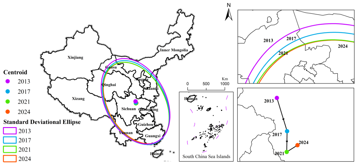
The standard deviational ellipse and centroid migration trajectory of logistics resilience in the NWLSC are shown in Figure 2.
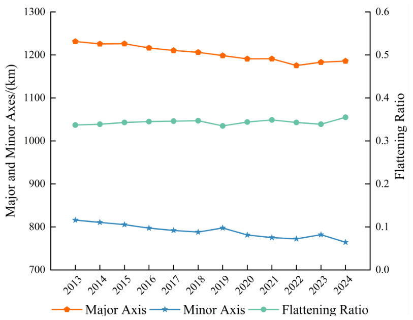
Moreover, Figure 3 presents the changes in the major axis, minor axis, and flattening ratio of the standard deviational ellipse, while Table 7 quantitatively lists the centroid coordinates, area, major axis, minor axis, flattening ratio, and other indicators of the standard deviational ellipse.
According to Figure 2 and Figure 3, the spatial distribution of logistics resilience in the NWLSC exhibits an evolutionary trend of a strengthened agglomeration, stable direction, and reinforced main axis. The spatial pattern has been continuously optimized under the guidance of core hubs and key corridors, yet regional imbalance still exists.
From the perspective of the distribution scope and agglomeration–dispersion, the ellipse area declined from 3.15581 million km2 to 2.84728 million km2 from 2013 to 2024, illustrated in Table 7. The major axis declined from 1231.325 km to 1185.786 km, and the minor axis dropped from 815.862 km to 764.368 km, as shown in Table 7, indicating that logistics resilience exhibits a certain degree of spatial convergence and agglomeration.
From the perspective of directional change and morphological stability, the azimuth angle of the standard deviational ellipse varied slightly, adjusting from 151.836° to 150.071°, illustrated in Table 7. The overall spatial distribution maintained a northwest–southeast direction with only minor optimization. Meanwhile, the flattening ratio rose from 0.337 to 0.355, shown in Table 7. This indicates that the logistics resilience still exhibits a certain degree of directional agglomeration, and this directionality has not been weakened.

4.1.3. Centroid Migration Trajectory

As shown in Figure 2, the centroid of logistics resilience has successively displayed a phased migration trend of southeastward deviation–northeastward extension.
From the perspective of the centroid location and migration characteristics, the spatial centroid of logistics resilience in the NWLSC has always been located within Sichuan Province, shifting continuously southeastward from 2013 to 2021 and then turning to northeastward migration from 2021 to 2024.
From the perspective of the migration distance and direction of the logistics resilience centroid, the centroid moved a total of 67.988 km, with an average annual migration of approximately 5.665 km. Among them, the centroid migration speed was the fastest from 2013 to 2017, with a migration distance of 34.659 km.

4.2. Structural Evolution of the Spatial Correlation Network

This subsection applies the inter-provincial spatial correlation intensity to visually illustrate the structure of the logistics resilience spatial correlation network in the NWLSC. Then, using the UCINET software, empirical analyses are conducted across three hierarchical dimensions, the overall network properties, individual node functional status, and block clustering configurations, which reveal the network evolutionary patterns, nodal functional heterogeneity, and inter-block spillover effects.

4.2.1. Structure of Spatial Correlation Network

According to the measured logistics resilience of the NWLSC, the modified gravity model is adopted to calculate the inter-provincial spatial correlation intensity of the logistics resilience. Binary discretization is then conducted to obtain the spatial adjacency matrix, with which the logistics resilience spatial correlation network is established.
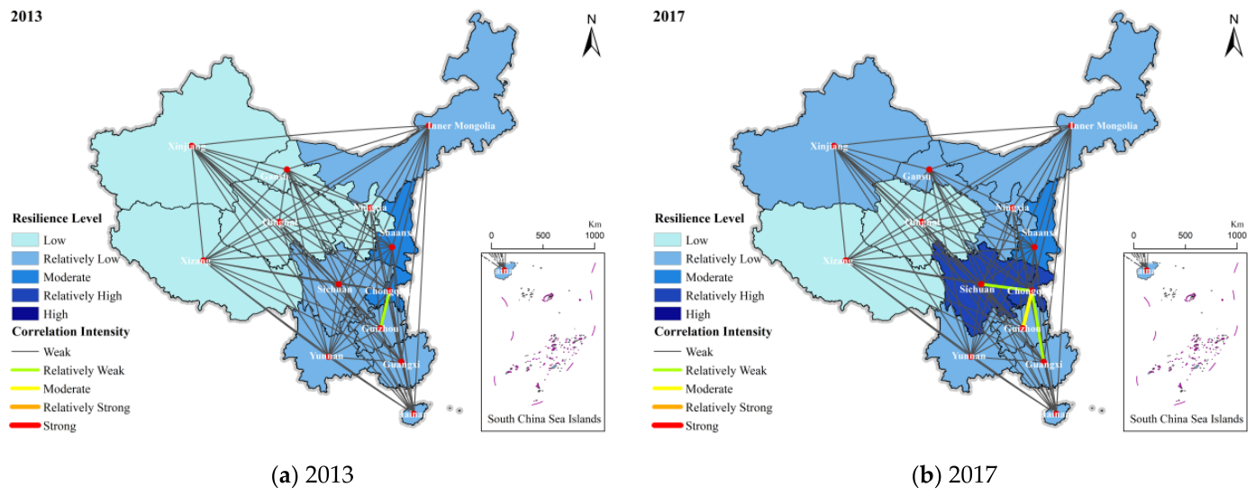
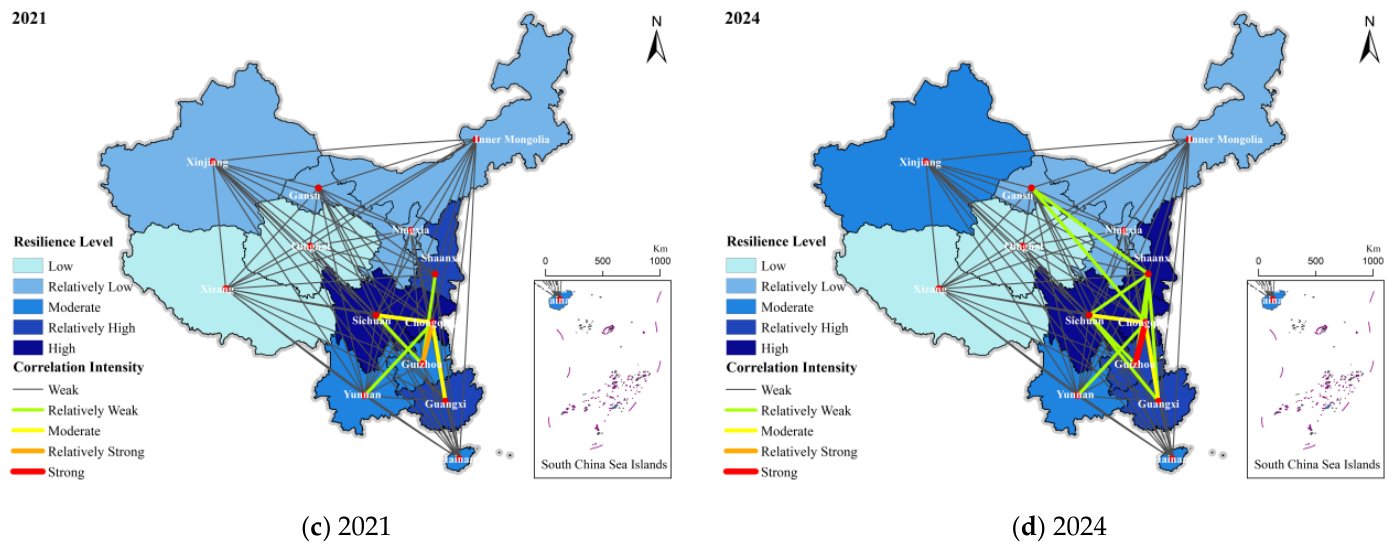
The natural breaks method is used for classification, and ArcGIS 10.8 is employed to depict the spatial network structure graph of logistics resilience and spatial correlation intensity, as shown in Figure 4.
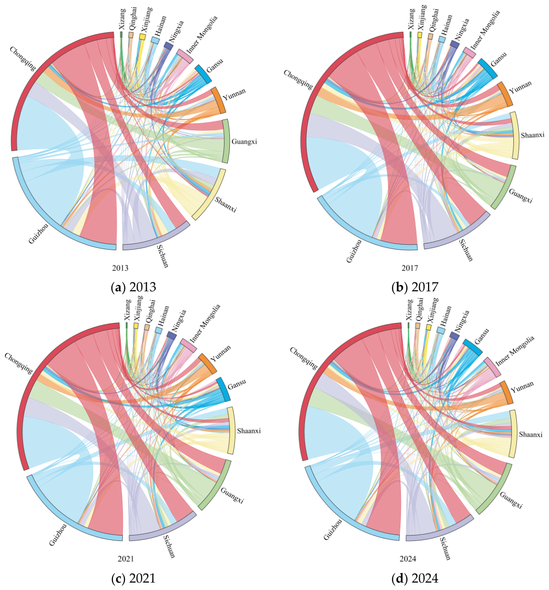
According to the gravity matrix, a chord diagram is further plotted by Origin to demonstrate the intensity and direction of the spatial correlation among provinces, as illustrated in Figure 5.
From Table 5 and Table 7, it is clear that, since the issuance and implementation of the Master Plan for the New Western Land–Sea Corridor in 2019, the logistics resilience has improved significantly, with substantial spatial disparities. Chongqing, Sichuan and Shaanxi enjoy distinct advantages, whereas Qinghai and Xizang are relatively underdeveloped. Chongqing is positioned as the logistics operational center of the NWLSC, and is also a newly planned national central city, the first national five-type logistics hub and the shipping center in the upper reaches of the Yangtze River, supported by multiple policy advantages. As one of the dual cores of the Chengyu Twin-City Economic Circle, Sichuan is also part of the cores of the NWLSC, with prominent locational advantages supported by developed industries and a concentrated population. Shaanxi is a traditional distribution hub in western China, with access to Europe and Asia toward the north and west, access to the sea via Chongqing, Guizhou and Guangxi toward the south, and access to the sea via North China toward the east, featuring high traffic accessibility. Qinghai and Xizang are located on the plateau, where underdeveloped economies and industries lead to a relatively low level of logistics resilience.
From the natural breaks classification of correlation intensity in Figure 4 and the visualization of the correlation direction in Figure 5, the logistics resilience in the NWLSC presents significant spatial correlation. Inter-provincial spatial correlation has broken through geographical adjacency and formed a stable hierarchical structure of operation center–corridor hub–trade gateway. Even the relatively underdeveloped Qinghai and Xizang maintain various connections with other provinces, though the intensity is relatively weak. The correlation intensity centered on Chongqing is particularly prominent, and strong linkages exist between Chongqing and Guizhou, Sichuan and Guangxi, reflecting the typical organizational chain of inland hub–communication artery–southbound maritime gateway. As an upstream supply and industrial hinterland, Sichuan agglomerates toward Chongqing, is conveyed through corridor sections such as Guizhou, and then is distributed intensively to maritime gateways such as Guangxi, forming a high-frequency and strongly coupled resilience linkage in the network. In addition, Chongqing, as the logistics operational center of the NWLSC, has continuously improved its status in the general spatial network, while Guangxi, as the southbound maritime gateway, has also achieved remarkable enhancement.

4.2.2. Evolution of Overall Network Properties

Five indicators, including network density, network relationship count, network connectedness, network hierarchy, and network efficiency, are adopted to depict the overall structural properties and evolutionary characteristics of the spatial correlation network, whose specific values are calculated with UCINET and then listed in Table 8.
According to Table 8, three key findings emerge from the evolution tendency of the overall network. First, the overall network accessibility is strong with no isolated nodes. From 2013 to 2024, the network connectedness maintained a value of one, illustrating that there were not any isolated and unreachable nodes in the network. All provinces were embedded in the same connected system, providing a solid structural foundation for inter-provincial coordination. Second, the network scale and density generally show an evolutionary trend of recovery amid fluctuations and enhancement during recovery. The number of network relationships fluctuated slightly around 50. Affected by external shocks, the number dropped significantly to 45 in 2020, then gradually rebounded and reached a peak of 53 in 2024. Meanwhile, the network density changed synchronously and reached its maximum value of 0.340 in 2024. Third, the network stability has undergone an adjustment from a rigid hierarchy to redundant backup. The network hierarchy remained unchanged at 0.500 from 2021 to 2022, and dropped to 0.400 in 2023 and 2024. Network efficiency hit its overall peak at 0.652 in 2020, while falling to 0.576 in 2024. Then, the alternative channels and shock-resisting buffer had strengthened.

4.2.3. Evolution of Individual Nodal Functional Status

The three core centrality indicators of degree centrality, closeness centrality, and betweenness centrality are adopted to identify the individual functional status of each provincial node. The standardized percentages are listed in Table 9, where the four years of 2013, 2017, 2021, and 2024 help illustrate the dynamic trends.
(1)
Degree Centrality: Direct Connectivity and Core Status
From Table 9, the average degree centrality for the four selected years is 51.282, 48.718, 48.718, and 51.282, respectively. Clearly, the Main Channel provinces are always significantly above average, which verifies their central statuses within the spatial network.
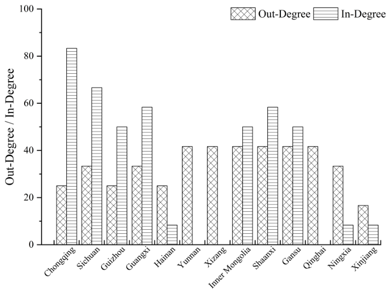
Furthermore, the specific out-degree and in-degree of each provincial region in 2024 are listed in Figure 6 in detail. Chongqing has the highest degree centrality. Sichuan, Shaanxi, Gansu and Inner Mongolia maintain strong connectivity. Thus, they have direct correlations with more nodes and possess stronger capabilities in receiving and spilling over production factors within the network. As the operational center of the corridor and a key national logistics hub, Chongqing undertakes functions such as train schedule arrangement, multimodal transport connection and resource coordination, thus establishing stable bidirectional correlations. Supported by developed industries and a large population, Sichuan continuously supplies cargo sources and logistics demands, enabling it to maintain a high level of connectivity in the spatial network. On the contrary, Ningxia, Xinjiang and Hainan show relatively low degree centrality, which means they have limited direct connections with others. Restricted by natural conditions, economic foundation and geographical location, they mostly act as terminal undertakers and peripheral nodes in the network.
(2)
Closeness Centrality: Accessibility and Network Position
From Table 9, the mean values of closeness centrality in the selected four years are 68.035, 67.577, 67.430, and 68.012, respectively. Analogous to the above case of degree centrality, the Main Channel provinces are always significantly above average. They have distinct locational advantages within the spatial network. Comparatively, they can connect more nodes via fewer intermediaries because of shorter path lengths, which facilitates trans-regional cooperation.
In terms of provincial-level regions, Chongqing, Inner Mongolia, Sichuan, Shaanxi, Gansu, and Guangxi rank sequentially in 2024. Chongqing and Sichuan connect the hinterland and outward systems, boasting stronger linkage and resource coordination capabilities, thus achieving shorter reachable distances in the network. Inner Mongolia functions as a pivotal hub in the north with a relatively compact connection structure with multiple regions, hence presenting high overall accessibility. Shaanxi and Gansu are located in the segments linking northwest, southwest, inland and border areas, and undertake corridor-type connecting functions for cross-sector and cross-regional ties, enabling them to maintain high reach efficiency in numerous shortest paths. As a sea outlet gateway facing ASEAN, Guangxi acts as a node for inland distribution and maritime external linkage, maintaining frequent interactive connections with many nodes, which facilitates it to occupy highly accessible positions in the network. In contrast, Hainan and Xinjiang exhibit relatively low closeness centrality. Their connections with other regions require traversing multiple intermediate nodes, resulting in longer average shortest paths. This positions them as classic peripheral nodes within the network.
(3)
Betweenness Centrality: Intermediary Power and Bridge Function
From Table 9, the average betweenness centrality for the four selected years is 5.711, 6.469, 5.420, and 5.944, respectively. Different from the previous two indicators, it is the Extended Belt instead of the Main Channel provinces that are above average, demonstrating their important roles as intermediaries and bridges.
In terms of provincial-level regions, Gansu, Shaanxi, Inner Mongolia, and Guangxi rank sequentially in 2024. Gansu is endowed with formidable intermediary control power since the Hexi Corridor serves as an irreplaceable overland passage linking China’s interior with Xinjiang and Central Asia. Shaanxi relies on the national comprehensive transportation status of hubs such as Xi’an to connect multidirectional flows to the northwest, central and eastern regions. Inner Mongolia links up with Eurasia to the north and west, and gains maritime access via Northeast and North China in the east and through Shaanxi, Chongqing, Guizhou and Guangxi in the south, acting as a key transit hub for inter-regional connections. Guangxi undertakes the transit function of converting inland distribution and transportation into cross-border maritime operations. Conversely, Yunnan, Xizang, Qinghai, and Xinjiang show low betweenness centrality, meaning they are rarely situated on the shortest paths between pairs of other provincial nodes. This indicates their limited capacity to mediate inter-provincial logistics flows, which is consistent with their edge-node positioning concluded from centrality analysis.

4.2.4. Evolution of Block Clustering Configurations

Block modeling with the CONCOR algorithm in UCINET was applied to further explore the network’s spatial clustering configurations and inter-block functional division. The 13 provinces were divided into four blocks. The following analyzes the clustered blocks, role evolution, spillover effects, and visualized spillover relationships, with a focus on temporal changes and 2024 cross-sectional characteristics.
(1)
Clustered Blocks
Table 10 presents the results of block clustering in 2013, 2017, 2021, and 2024, including the received, spilled, and intra-block relations and block type classification.
In 2024, the total number of network relationships in the logistics resilience spatial correlation network is 53, with 10 intra-block relationships and 43 inter-block relationships. The functional characteristics of each block are as follows:
Block I (Bidirectional Spillover Block: Inner Mongolia and Xinjiang): Balanced incoming (six) and outgoing (six) inter-block relations, with one intra-block relation (actual internal ratio = 14.29% > expected 8.33%).
Block II (Net Spillover Block: Ningxia, Qinghai, Xizang, Gansu, and Yunnan): Few incoming inter-block relations (four) but abundant outgoing relations (21), with three intra-block relations (actual internal ratio = 12.50% < expected 33.33%).
Block III (Broker Block: Guangxi and Guizhou): More incoming inter-block relations (13) than outgoing (seven), with zero intra-block relations (actual internal ratio = 0.00% < expected 8.33%).
Block IV (Net Beneficiary Block: Hainan, Chongqing, Shaanxi, and Sichuan): Abundant incoming inter-block relations (20) but few outgoing (nine), with six intra-block relations (actual internal ratio = 40.00% > expected 25.00%).
(2)
Role Evolution
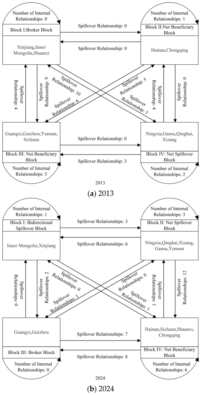
The clustering blocks evolved sharply from 2013 to 2024, shifting from the pattern of “brokers supporting multiple beneficiaries” to the pattern where net beneficiaries act as core absorbing nodes, brokers serve as key links, net spillovers function as major supply ends, and bidirectional spillovers engage in two-way connections. For example, this can be seen in Xinjiang and Inner Mongolia (2013: broker → 2024: bidirectional spillover); Shaanxi (2013: broker → 2024: net beneficiary); Guangxi and Guizhou (2013: net beneficiary → 2024: broker); and Yunnan (2013: net beneficiary → 2024: net spillover).
(3)
Spillover Effects
On the basis of block clustering, both the density matrix and corresponding image matrix of the above four blocks are calculated to reveal the spillover relationships among blocks. First, the density matrix is obtained via the CONCOR module, adopting the iterative convergence method in the UCINET software. Then, taking the overall annual network density in Table 8 as the threshold, the density matrix is binarized to acquire the corresponding image matrix, as summarized in the following Table 11.
In 2013, the spillover pattern was dispersed: Block I exerted spillover to Block III; Block II maintained both internal self-cycles and spillover to Block III; Block III had internal self-cycles and exerted spillover to Block II; and Block IV generated spillover to both Block I and Block II.
By 2024, a clear, hierarchical spillover structure emerged: Block I maintained internal self-cycles and exerted spillover to Block III; Block II exerted spillover to both Block I and Block IV; Block III generated spillover to Block IV; and Block IV sustained both internal self-cycles and exerted spillover to Block III.
(4)
Visualized Spillovers
To intuitively illustrate the directional spillover flows, the inter-block spillover relationships in 2013 and 2024 are visualized in Figure 7 with relational counts quantifying the intensity of each linkage.
In 2013, Block I is not endowed with internal relations and receives 14 incoming spillover relations (4 from Block III and 10 from Block IV). It generates 12 outgoing spillover relations (9 to Block III and 3 to Block IV). Block II has only one internal relation and receives nine incoming spillover relations (five from Block III and four from Block IV). It generates six outgoing spillover relations (all to Block III). Block III has five internal relations and receives 18 incoming spillover relations (9 from Block I, 6 from Block II, and 3 from Block IV). It generates nine outgoing spillover relations (four to Block I and five to Block II). Block IV has two internal relations and receives three incoming spillover relations (all from Block I). It generates 17 outgoing spillover relations (10 to Block I, 4 to Block II, and 3 to Block III).
In 2024, Block I is endowed with only one internal relation and receives six incoming spillover relations (all from Block II). It generates six outgoing spillover relations (three to Block II, two to Block III, and one to Block IV). Block II has three internal relations and receives four incoming spillover relations (three from Block I and one from Block IV). It generates 21 outgoing spillover relations (6 to Block I, 3 to Block III, and 12 to Block IV). Block III has no internal relations and receives 13 incoming spillover relations (2 from Block I, 3 from Block II, and 8 from Block IV). It generates seven outgoing spillover relations (all to Block IV). Block IV has six internal relations and receives 20 incoming spillover relations (1 from Block I, 12 from Block II, and 7 from Block III). It generates nine outgoing spillover relations (one to Block II and eight to Block III).

4.3. Driving Mechanism of the Network Structure Evolution

4.3.1. Variable Selection

In order to identify the driving mechanism for the structural evolution of the spatial correlation network with the QAP model, the following potential factors are selected as possible explanatory variables:
Economic development (X1), characterized by the difference matrix of per capita regional GDP; inclusive finance (X2), characterized by the difference matrix of the Inclusive Finance Index released by Peking University; environmental pollution governance (X3), characterized by the difference matrix of the ratio of fiscal environmental protection expenditure to fiscal budget; educational advancement (X4), characterized by the difference matrix of the ratio of the number of students in regular institutions of higher education to the total population; industrial structure rationalization (X5), characterized by the difference matrix of the industrial Theil index; urbanization level (X6), characterized by the difference matrix of the ratio of urban population to permanent population; technological innovation (X7), characterized by the difference matrix of the ratio of the number of three types of patent authorizations to the permanent population; informatization level (X8), characterized by the difference matrix of the number of websites per 100 enterprises; and geospatial proximity (X9), characterized by the geographic adjacency matrix between provincial capitals.
We convert the above eight difference matrices into binary form using row mean differences as the threshold. A value of one is assigned when the inter-provincial difference is above the row mean, indicating a large disparity, and zero otherwise. These binary matrices and the geographic adjacency matrix are the relational matrices used as independent variables in the QAP model. Actually, constructing attribute-difference matrices as QAP independent variables follows the standard dyadic-regression practice established by references [43,44,45]. Furthermore, the choice to binarize these difference matrices by focusing on whether the gap between two units exceeds the typical disparity observed across the network—rather than on the precise magnitude of the gap—is widely adopted. For instance, several urban and regional network studies define relational ties by whether a dyad exceeds a systemic norm [46,47]. In particular, the row mean is used as the threshold in [48,49] to convert continuous attribute matrices into binary ones, whereas median and fixed-percentile thresholds, by ignoring within-row value heterogeneity, may bias the dyadic relational structure embedded in permuted matrices and thus distort the QAP inference. Accordingly, we adopt the row-mean thresholding procedure for binarization.

4.3.2. QAP Correlation Analysis

The logistics resilience spatial correlation network is presented in matrix form. Therefore, it is difficult to effectively analyze the relationships between such matrices with traditional statistical analysis methods because high correlation exists among explanatory variables. To avoid multicollinearity, the non-parametric QAP model is adopted to identify the driving factors of the logistics resilience spatial correlation network in the NWLSC.
The correlations between the explanatory and explained variables are obtained through 5000 random permutations, and the final results are illustrated in Table 12.
The QAP correlation analysis results illustrate that the structure of the logistics resilience spatial correlation network in the NWLSC is significantly influenced by factors such as economy, geography, education, and technology. Specifically, both economic development and educational advancement reach significance at the 1% statistical level; geospatial proximity and technological innovation reach it at the 5% statistical level; and urbanization level reaches it at the 10% statistical level; all five variables exhibit a positive correlation. In contrast, the inclusive finance, environmental pollution governance, industrial structure rationalization, and informatization level all show no statistical significance.

4.3.3. QAP Regression Analysis

The QAP regression model is employed to identify the driving factors behind the structural evolution of the logistics resilience spatial correlation network in the NWLSC. According to Equation (13), the econometric model is:
L R = β 0 + β 1 X 1 + β 2 X 2 + β 3 X 3 + β 4 X 4 + β 5 X 5 + β 6 X 6 + β 7 X 7 + β 8 X 8 + β 9 X 9 + E
L R represents the gravity-based adjacency matrix of logistics resilience across provinces in the NWLSC; X denotes the relational matrix corresponding to each explanatory variable; β denotes the regression coefficient of each explanatory variable; and E represents the random error term.
Then, this model is adopted to identify the driving effects of various factors while controlling for other variables, and the regression results are achieved through 5000 random permutations, as illustrated in Table 13.
In terms of model specification, the adjusted R2 is 0.384 at a significance level of 0.001, indicating that the model setting is reliable. These nine influencing factors can totally explain 38.4% of the variation in the spatial linkages of logistics resilience in the NWLSC.
In terms of specific influencing factors, there is significant heterogeneity in the regression results across different variables. Economic development (X1) and geospatial proximity (X9) both reach the 1% statistical significance level, and educational advancement (X4) reaches the 5% statistical significance level. Each of the three statistically significant variables carries a positive regression coefficient. In detail, the standardized regression coefficient of economic development (X1) is 0.523, while those of geospatial proximity (X9) and educational advancement (X4) stand at 0.299 and 0.150, respectively. However, inclusive finance (X2), environmental pollution governance (X3), industrial structure rationalization (X5), urbanization level (X6), technological innovation (X7), and informatization level (X8) all lack statistical significance, as they do not pass the significance test.

5. Discussions

5.1. Decoding the Spatial Logic of Logistics Resilience Growth

5.1.1. Policy Cycles: Accelerating Resilience and Gradient Differentiation

On one front, a pronounced policy-driven effect emerges in the process of the consistent improvement of logistics resilience. Three distinct growth peaks appear in 2019, 2021 and 2024, closely matching the rollout of core institutional policies. In 2019, the Master Plan for the NWLSC was released, which established the overarching framework of delineating strategic directives regarding positioning, hub network layouts, key project construction, and collaborative operational mechanisms. In 2020, the outbreak of COVID-19 disrupted logistics networks, and the inherent vulnerabilities within the logistics system were fully exposed. In 2021, the Implementation Plan for High-Quality Development of the NWLSC during the 14th Five-Year Plan Period outlined concrete measures focusing on infrastructure upgrades, efficiency optimization, and enhancement of multimodal transport coordination. The Regional Comprehensive Economic Partnership (RCEP), effective in 2022, incorporated the corridor into global value chains and boosted China–ASEAN economic links and freight volumes, whose dividends became fully evident by 2024.
On the other front, the policy-driven effect shows prominent regional heterogeneity. The improvement of logistics resilience varies across provincial-level regions, and the Main Channel provinces serve as the growth pole driving sequential resilience elevation along the whole corridor. Such spatial differentiation results from the integration of national strategic plans, geographical resource endowments, and locational conditions. National strategies offer long-term guidance and an institutional guarantee for the evolution of logistics resilience, while such evolution is also restricted by geographical endowments and location advantages. Developed regions including Chongqing and Shaanxi maintain robust logistics resilience thanks to mature corridor operation systems, well-planned hub distribution and stable large-scale market demand supported by population agglomeration and economies of scale. By contrast, the underdeveloped regions such as Qinghai and Gansu are restricted by a small market scale, backward infrastructure and inferior geographical conditions, whose improvement of logistics resilience thus depends largely on external resource input.
Summarily, although the logistics resilience has kept a steady increasing tendency, the growth is driven mostly by top-down policy incentives instead of spontaneous endogenous engines. Furthermore, such policy-driven dynamics have a typical character of regional heterogeneity, which manifests as a distinct pattern of gradient differentiation across provincial-level regions.

5.1.2. Geographic Inequality: Hub Dominance with Peripheral Dependence

The long-term gradient disparity in logistics resilience displays a distinct core–periphery spatial hierarchy. Core regions have been accumulating development dividends, whereas peripheral regions still continuously rely heavily on external support, which greatly deviates from the goal of balanced development. Chongqing, Sichuan and Shaanxi, as typical—key regions, maintain strong logistics resilience and rapid growth because of their advantages in superior hub locations, solid industrial foundations and scale economies, which actually have formed a self-reinforcing virtuous cycle. In contrast, Gansu, Qinghai and Xizang, as typical peripheral areas, have been stuck in a low-development and low-growth pattern, and their resilience improvement is dominated by external capital investment rather than endogenous driving forces. However, current policies have solidified the spatial hierarchical structure and have not effectively narrowed regional gaps. The spatial agglomeration effect of logistics resilience keeps strengthening, while the trend of agglomeration becomes stable, and the main axis becomes increasingly distinct, which reflects an evolutionary regional imbalance.
On the one hand, variations in the coverage scope and principal axes of the standard deviational ellipse verify that the spatial hierarchy of logistics resilience evolves from a dispersed state to an agglomerated pattern. With the shrinking elliptical coverage and the shortening of both major and minor axes, the overall spatial layout tends to be increasingly consolidated. Such spatial contraction is attributed to the leading driving effect of core hub regions because of their prominent advantages in operational efficiency and infrastructure network construction, which aligns with the practical development logic that prioritizes resource allocation and key construction investment in core nodes.
On the other hand, variations in the azimuth angle and oblateness ratio of the standard deviational ellipse illustrate a stable northwest–southeast agglomeration trend. Slight fluctuations occur in the azimuth while the oblateness ratio remains stable, which maintains a solid spatial layout along the axis without any diffusive tendency. This spatial differentiation reflects a non-equilibrium expansion mode that mainly relies on existing hub cities. Therefore, it is unnecessary to change the established agglomeration orientation to mitigate regional imbalances within the corridor. Instead, emphasis should be placed on improving the spillover transmission mechanisms of core hubs and strengthening their horizontal linkages with the corridor’s primary axis.

5.1.3. Centroid Dynamics: From Concentration to Diffusion

The empirical results on the spatial gravity center migration of logistics resilience show that the gravity center has long been situated in Sichuan Province, and there is a clear trajectory that it was initially concentrated in the Chengdu–Chongqing Area and then gradually extended northeastward.
This migration trajectory is highly consistent with the policy cycles. From 2013 to 2021, the orientation of the gravity center’s southeastward movement verifies that the Chengdu–Chongqing Twin-City Economic Circle steadily consolidated itself as the growth pole because of sound manufacturing foundations and integrated transportation facilities. After 2021, the northeastward shift indicates that Chongqing and Sichuan have strengthened spatial radiation effects and factor diffusion enough to spill over to the primary axes such as Shaanxi.
In particular, the migration develops with high speed at the early stage, which is also propelled by multiple major policies. For example, in 2013, the Belt and Road Initiative was launched, which built a strategic framework for cross-regional connectivity; in 2014, the Medium and Long-Term Logistics Development Plan was released, which clarified the modernization objectives of logistics infrastructure and multimodal transportation; and in 2015, the implementation effect of the China–Singapore Connectivity Initiative was manifested. The combined effects of these policies granted advantages to core hub cities, facilitated the directional agglomeration of logistics resilience, and further promoted the spatial shift of its gravity center.
Overall, the spatial configuration of logistics resilience within the NWLSC features concentrated distribution, stable evolutionary trends and orderly gravity center migration. Despite the ongoing optimization of the spatial structure, there are still prominent regional imbalances. Accordingly, it is essential to reinforce horizontal inter-regional connections and factor spillover mechanisms, so as to guide the evolution of corridor logistics resilience toward more coordinated, equitable, efficient and high-quality development.

5.2. Unpacking the Spatial Architecture of the Logistics Resilience Network

5.2.1. Hierarchy and Specialization in Network Topology

The above network topology and chord diagram analyses demonstrate that logistics resilience within the NWLSC presents prominent spatial network linkages, which have formed a robust hierarchical system composed of operational nodes, corridor hubs, and outward-facing gateways. Notably, these inter-provincial interactive correlations extend beyond simple geographical adjacency.
Provincial-level regions show clear functional differentiation with dominant core nodes and loosely connected peripheral ones. For example, Chongqing, which is designated as the corridor’s core operational center and national comprehensive logistics hub, lies at the network core nexus, coordinates regional logistics operations and shapes a prominent spatial Chongqing-centered agglomeration pattern. Sichuan, as part of the Chengdu–Chongqing Twin-City Economic Circle, builds an inland-sea-linked logistics framework by conducting logistics transshipment via Guizhou and connecting global markets through Guangxi. Shaanxi, as a traditional northwest distribution hub, facilitates multidirectional connectivity, which extends westward to Eurasia and southward to maritime routes linking Asia, America, and Europe. Qinghai and Xizang still present weak network links amid expanding overall network scales and tighter connections. However, tangible infrastructure connectivity has not yet been fully translated into effective functional integration because physical infrastructure cannot achieve spontaneous functional synergy without effective policy guidance and institutional guarantees.
In summary, driven by policy guidance and functional positioning, the structural configuration of the logistics resilience network within the NWLSC has been steadily optimizing. In particular, Chongqing remains in a leading position in network centrality while Guangxi further solidifies its status as a maritime gateway.

5.2.2. Overall Resilience as a Function of Network Redundancy

In terms of Network Connectivity, the corresponding indicator remained stable at one throughout 2013–2024. Such saturation means there are no any isolated nodes in the spatial correlation network. It also demonstrates a high level of integration, where all provincial-level regions are embedded within the single system of the NWLSC to support the functional synergy and spillover diffusion of resilience elements.
In terms of the network relationships and density, both indicators show a trend of fluctuating adjustment followed by steady recovery, verifying the strong risk resistance of the corridor. The decline in network relationships in 2020, caused by external shocks including the pandemic, was a normal response to external pressures rather than a systemic breakdown. It achieved continuous recovery in subsequent years and reached its highest level in 2024, fully reflecting its powerful self-recovery ability and structural optimization potential. Consistent with this trend, the network density changed in step with network relationships, which enhanced the overall compactness of the logistics network by deepening regional connections and expanding the radiation scope.
In terms of the network hierarchy and efficiency, the spatial correlation network has achieved transformative upgrading, evolving from a rigid hierarchical subordinate structure to an optimized framework with redundant backup functions. In 2020, affected by the pandemic, network efficiency rose sharply to 0.652, which exposed the structural fragility and excessive dependence on core pivotal nodes. By 2024, network efficiency dropped to 0.576, signifying a sound evolutionary trend toward the gradual formation of diversified alternative transportation routes and multi-level backup routes. Accordingly, the network has shifted from the traditional mode, emphasizing lean efficiency while neglecting risk resistance, to a resilient pattern featuring redundant risk buffering capacities. With diverse redundant connections, a long-term mechanism for the steady improvement of logistics resilience can be established by building multi-dimensional transportation paths, improving risk response buffers, and boosting operational stability and environmental adaptability effectively.
Nevertheless, the current level still remains relatively low. To remedy such structural defects, it is urgent to construct a network with multi-path connectivity and sufficient redundancy, so as to comprehensively enhance the risk resistance and sustainable development capacity of the logistics system in the NWLSC.

5.2.3. Node Heterogeneity Beyond Simple Centrality

There are significant disparities in various network centrality indicators, which reflect an obvious divergence in functional positioning within the network. The Main Channel provinces have prominent advantages in degree centrality, while the Extended Belt provinces enjoy betweenness centrality. Thus, targeted and differentiated risk prevention and governance policies should be formulated in accordance with functional positions. For example, Chongqing and Sichuan, as the representatives of core regions, should consolidate foundational supporting and leading roles, while Shaanxi and Gansu, as the representatives of transit-dominant regions, should reinforce peripheral safeguards.
(1)
Degree Centrality
The geographical conditions, industrial foundations, and resource endowments collectively shape the spatial distribution of degree centrality. The core regions dominate the direct linkages within the network and have consistently maintained prominent advantages in degree centrality. Chongqing, benefiting from its dual strategic status as the operational center of the corridor and a national comprehensive logistics hub, has enabled efficient two-way logistics coordination via the China–Europe Railway Express, the organization of multimodal transportation, and cross-regional resource integration. Sichuan, based on the robust and stable logistics demand stemming from its solid industrial foundation and large population, boasts prominent strength in network interconnectivity. In contrast, peripheral regions register relatively low degree centrality and occupy marginal and terminal positions within the network. For example, Ningxia, Xinjiang and Hainan act as typical peripheral nodes with weak capabilities in direct inter-regional logistics connectivity because of their remote geographical locations, simplistic economic structures or insufficient resource endowments, which collectively impose substantial constraints on their logistics resilience.
(2)
Closeness Centrality
The positional status of a single node in the spatial network is characterized by the indicator of closeness centrality. Hub nodes boast prominent advantages and occupy favorable network positions that support efficient inter-regional cooperation via fewer transit links. Chongqing and Sichuan, relying on the national policy of the Chengdu–Chongqing Twin-City Economic Circle, actually have built a logistics network connecting inland hinterlands with global markets. Shaanxi and Gansu, driven by the Belt and Road Initiative, act as pivotal channels that strengthen the connectivity between inland and border areas. Guangxi, as the southern maritime gateway, facilitates unobstructed cargo transportation from inland China to ASEAN. Inner Mongolia, endowed with multidimensional transportation passages, promotes the integrated development of the spatial network. In comparison, peripheral nodes are constrained by redundant intermediate connections and thus exhibit relatively low efficiency. For example, Hainan and Xinjiang record relatively low closeness centrality. Their logistics transportation features longer shortest paths and heavy dependence on multi-level intermediate node connections, which further demonstrates their peripheral positioning within the spatial network.
(3)
Betweenness Centrality
Reflecting the bridging intermediary role of nodes, betweenness centrality highlights the core significance of transit hubs. The Extended Belt provinces score highly in this indicator, which demonstrates their irreplaceable function in facilitating factor mobility and linking different parts of the network. Specifically, Shaanxi, Gansu and Inner Mongolia stand out as key transit hubs. Shaanxi coordinates cross-regional factor flows heading north, west and south. Gansu, with the Hexi Corridor, acts as a vital overland transportation channel, while Inner Mongolia provides omnidirectional transport passages. Additionally, Guangxi enables efficient consolidation of inland goods and maritime foreign trade shipment, and hence registers a relatively high betweenness centrality, too. Conversely, Yunnan, Xizang, Qinghai and Xinjiang, with a limited capacity to coordinate cargo transshipment, record notably lower betweenness centrality, which is consistent with their peripheral roles in the network.

5.2.4. Block Dynamics of a Tributary System

Block configuration analysis reveals a marked evolution from basic point-to-point connections to a stable complex spatially correlated system. Notably, inter-block factor spillover links total 43 pairs, far exceeding the 10 intra-block pairs. Such disparity indicates that the network has entered a highly integrated development phase.
(1)
Clustered Blocks
Inter-block connections dominate spatial correlation in the logistics resilience network. A distinct functional division among blocks greatly improves network resource allocation efficiency. In 2024, inter-block linkages amounted to 43 pairs, taking up 81.13% of the overall 53 connections. This reflects high network integration, with cross-block factor spillover and transmission serving as the main spatial correlation pattern. Additionally, each block’s functional position matches its development orientation. Block I presents bidirectional spillover, featuring balanced factor absorption and outward diffusion. Block II shows net spillover, acting mainly as a factor supplier. Block III possesses broker properties, acting as an interconnection bridge. Block IV shows net beneficiary characteristics, functioning primarily as a center for factor convergence and absorption.
(2)
Role Evolution
The evolving roles of network blocks manifest the steady optimization of node functions amid changing policy orientations and development requirements in each development stage of the NWLSC. Changes in block agglomeration from 2013 to 2024 mirror the corridor’s remarkable advancement from strategic layout to mature operational status. Specifically, Xinjiang and Inner Mongolia have realized their transition to bidirectional spillover blocks, which reflects improved integration of cross-regional factor flows and the gradual maturation of the northbound channel construction. Shaanxi has achieved the shift toward a net beneficiary block, which is driven by the Belt and Road Initiative, the construction of the Xi’an–Xianyang Metropolitan Area, and the layout of national logistics hubs. The evolution of Guangxi and Guizhou into broker blocks corresponds to the gradual improvement of their maritime gateway and corridor segment functions. Yunnan’s transformation into a net spillover block is closely linked to its outward opening strategy toward Southeast Asia. These evolutionary changes collectively reflect the continuous optimization of the functional positioning of all regional nodes within the network.
(3)
Spillover Effects
The network’s transition from a dispersed spillover pattern in 2013 to a hierarchical spillover structure in 2024 reveals the increasing rationalization of the spatial correlation system. The clear cross-block spillover chains formed in 2024 further highlight the leading role of inter-block linkages in shaping logistics resilience. The shift from parallel multi-block connections to convergence centered on net beneficiary and broker nodes improves the overall network operational efficiency and coordinated development capacity. A comparative analysis of spillover patterns in 2013 and 2024 further confirms the structural optimization of the network. Block IV has evolved from a net spillover role into a core absorption node with strong internal cohesion, stabilizing overall network operation. Block II has developed into a major spillover supplier, enhancing the system’s proactive supply capacity. The overall transition from an unbalanced and externally dependent structure to a coordinated and self-sustaining system manifests the elevated integration level, structural stability, and high-quality development of the logistics industry.

5.3. Synthesizing the Spatial Drivers of the Evolutionary Network Structure

5.3.1. Rationale for Selecting Driving Factors

Generally, the selected nine factors cover economic, financial, environmental, educational, industrial, urbanization, technological, informatization and geographical dimensions, all of which are closely associated with the dynamic evolution of the logistics resilience spatial correlation network in the NWLSC.
Specifically, economic development creates basic logistics demand and provides financial support for transportation infrastructure construction. Inclusive finance helps fund infrastructure projects and grants credit access to logistics firms. Environmental pollution governance enforces emission limits and drives the industry’s green low-carbon transformation. Educational advancement cultivates professional logistics talents and improves industrial human capital. Industrial structure rationalization generates and meets logistics needs while lowering socioeconomic systemic risks. Urbanization boosts economies of scale and strengthens spatial agglomeration effects. Technological innovation raises operational efficiency via new facilities and cuts costs through management and institutional improvements. Informatization realizes cross-regional information sharing and breaks market segmentation barriers. Geographic proximity smooths commodity circulation and personnel communication, accelerating regional industrial and economic integration. Theoretically, these diverse factors impose significant influences on the structural evolution of the logistics resilience network.

5.3.2. Correlation Characteristics Between the Factors and Network

On the one hand, the QAP analysis reveals a significantly positive correlation between the evolution of the logistics resilience networks and five influencing factors, namely economic development, educational advancement, geographical proximity, technological innovation and urbanization, which verifies their pivotal role in driving structural changes in the spatial network. Specifically, economic development and educational advancement meet the 1% statistical significance threshold, and hence serve as primary driving forces that determine regional logistics demand levels and professional talent quality, respectively. Geographical proximity and technological innovation reach the 5% significance level, and hence lay a solid foundation for spatial coordination and technological upgrading, respectively. Urbanization satisfies the 10% significance threshold, which steadily strengthens the effects of factor agglomeration and the spillover of development benefits.
On the other hand, the QAP analysis illustrates four factors, including inclusive finance, environmental pollution governance, industrial structure rationalization and informatization, that fail to pass the correlation significance test. They do not manifest any direct influence autonomously, and their effects are contingent upon external mediating conditions instead of functioning independently.

5.3.3. Hierarchical Driving Effects and the Synergistic Mechanism

In terms of model specification, the adjusted goodness-of-fit value stands at 0.384, and the overall model passes the 0.1% significance test. These results prove the high reliability of the QAP regression model and demonstrate that the chosen driving factors can well explain the structural evolution of the spatial correlation network.
At the individual factor level, economic development, geographical proximity and educational advancement show statistically significant driving effects. The standardized regression coefficient of economic development (X1) reaches 0.523, revealing that economic conditions directly determine the freight demand scale and lay the fundamental foundation for logistics connections. For example, the sizable economy of the Chengdu–Chongqing Twin-City Economic Circle firmly consolidates its hub status in the NWLSC. Educational advancement (X4) obtains a coefficient of 0.150, implying that high-quality human resources provide essential soft power for logistics resilience. The stable supply of skilled practitioners and professional managers is critical to sustaining efficient and steady operation because modern logistics is a technology-and-management-intensive industry. Geographical proximity (X9) has a coefficient of 0.299, verifying that spatial distance acts as a basic network constraint and directly affects logistics time and transportation expenses. Empirical results indicate that logistics connections inside the Main Channel with compact adjacency are closer and better coordinated than those in the Extended Belt, featuring vast land coverage and longer spatial distances. By contrast, other factors such as inclusive finance and informatization show no statistical significance. This result deviates from conventional cognition and reflects the unique empirical value of this empirical study. Both correlation and regression analyses fail to validate their significance, which verifies that they cannot exert driving influence independently and their effects hinge on basic preconditions. For example, inclusive finance barely boosts logistics resilience in regions with weak industrial foundations, while informatization cannot effectively allocate logistics resources when the transportation network remains fragmented. Therefore, regional policymakers should implement policies to synchronize technological innovation, financial service improvement and industrial structure upgrading.
In summation, various influencing factors present distinct hierarchical disparities and form a synergistic mechanism dominated by economic growth, constrained by geographical conditions and supported by educational advancement. These drivers interact rather than work in isolation. Economy, geography and education serve as core impetuses, while technological innovation, financial services, informatization and urbanization further strengthen their effects. Such coordinated synergy facilitates the high-quality structural evolution of the spatial network.

5.4. Robustness Test

5.4.1. Robustness to Variations in the Distribution Coefficient

As derived via the game theory combined weighting method in Section 3.2, the distribution coefficient of CRITIC weights is 0.213, while that of weights from the improved entropy method is 0.787, and the corresponding results of logistics resilience in the NWLSC are listed in Table 5. When the distribution coefficients are adjusted to (0.3, 0.7), the results of the logistics resilience are presented in Table 14. By comparison, although the individual specific numerical values change to a certain extent, the relative magnitude of each value remains largely unchanged. In other words, the ranking of logistics resilience levels and growth rates across provinces in the NWLSC is basically consistent, which means that the spatial correlation matrix will remain unchanged.
Furthermore, when the distribution coefficients are reset to (0.4, 0.6) and (0.5, 0.5), the corresponding logistics resilience evaluation results are listed in Table 15 and Table 16, respectively. Similarly, by comparing the results with various distribution coefficients, it is clear that the relative relationships between all numerical values still stay nearly identical, and thus the relative order of logistics resilience and its growth rate for each province in the NWLSC remains stable.
Therefore, the spatiotemporal differentiation and structural evolution of the logistics resilience spatial correlation network in the NWLSC are robust to variations in the distribution coefficients.

5.4.2. Robustness to Variations in the Binarization Threshold

In Section 3.3, the average values were taken as the binarization threshold to convert the gravity matrix into a 0–1 binary gravity-based adjacency matrix. For each column in every row of the gravity matrix, if the gravity value of the column is larger than the average of the corresponding row, the gravity-based adjacency value is designated as one, or otherwise as zero. Since the binary gravity-based adjacency matrix serves as the fundamental prerequisite for subsequent social network analysis, different binarization thresholds may alter the overall structure of the logistics resilience spatial correlation network. In order to test the reliability of the binarization criterion, we adjusted the transformation benchmark by selecting the 65th quantile as the new threshold for matrix binarization. The overall structural characteristics and the individual nodal functional statuses of the reconstructed spatial correlation network under this new setting are summarized in Table 17 and Table 18, respectively.
Regarding the overall structural characteristics, by comparing the calculated indicators before and after adjusting the threshold in Table 16 and Table 17, we can clearly find that four out of five core indicators, namely network density, network connectedness, network hierarchy and network efficiency, maintain a relatively stable state on the whole. Although slight fluctuations exist in their specific numerical values, the relative size relationships between these indicators do not undergo obvious changes. Nevertheless, the indicator of network relationships presents a striking difference. Under the 65th quantile threshold, it is fixed at 52 for each year over the study period, instead of fluctuating up and down around 52 as it did when the mean value was adopted as the transformation standard. This regular difference is fundamentally determined by the inherent attributes of the quantile segmentation criteria. When a quantile is set as the binarization benchmark, the ranking of elements within each row of the gravity matrix varies from year to year, which will alter the specific positions of elements equal to one in the binary gravity-based adjacency matrix. However, the total quantity of elements equal to one in the whole matrix will stay constant. On the whole, the overall structural features of the spatial correlation network do not experience substantive shifts even if the binarization benchmark is replaced with the 65th quantile.
Regarding the individual nodal functional status, by comparing the calculated indicators before and after adjusting the threshold in Table 17 and Table 18, we can clearly find that all the three core indicators, namely degree centrality, closeness centrality, and betweenness centrality, stay largely consistent overall. Even though their concrete values fluctuate slightly, the relative ordering of the indicators barely changes.
Furthermore, if the 60th and 70th quantiles are taken as the binarization thresholds, the results are highly similar to the above case of the 65th quantile. Therefore, we can conclude that the research conclusions derived from the spatial correlation network analysis, such as the overall network properties and individual nodal functional statuses, are robust to different choices of the binarization threshold to a large extent.

5.4.3. Robustness to Variations in Year Windows

The study period adopted for the QAP analysis spans from 2013 to 2024, covering 12 years. However, this time frame cannot be extended to earlier years due to limited data availability, as several statistical indicators are missing in the early stage, especially those measuring the development of information technology.
Frequent COVID-19 outbreaks occurred between 2020 and 2022, and effective isolation and epidemic prevention control measures were widely implemented nationwide, which exerted remarkable impacts on the transportation and logistics industries. In order to eliminate the interference caused by this special exogenous shock, we excluded the samples from 2020 to 2022 and re-performed the QAP analysis. The correlation results are displayed in Table 19, and the regression results are listed in Table 20.
Regarding the QAP correlation analysis, by comparing Table 12 and Table 19, it is clear that after removing the samples from the COVID-19 years, only slight variations exist in the specific values of correlation coefficients. Economic development X1, educational advancement X4, urbanization X6, technological innovation X7 and geospatial proximity X9 remain statistically significant. Specifically, the significance level of educational advancement X4 decreases from 1% to 5%, whereas the significance level of urbanization X6 rises from 10% to 5%. Overall, the QAP correlation analysis is robust to year windows with and without COVID-19.
Regarding the QAP regression analysis, by comparing Table 13 and Table 20, it is clear that economic development X1 remains statistically significant at the 1% significance level after removing the samples from the COVID-19 years. However, obvious variations emerge, although minor differences can be observed in the specific values of the correlation coefficients. Educational advancement X4 is no longer significant, whereas technological innovation X7 becomes significant. In other words, COVID-19 altered the QAP regression results by rendering educational advancement X4 insignificant and technological innovation X7 significant. One plausible reason is that the isolation and control measures implemented during the pandemic restricted or even disrupted transportation and logistics, yet the provision of education merely shifted online rather than coming to a halt. Additionally, the adjusted R2 decreases from 0.384 to 0.362 because the shorter sample period without the pandemic years leads to a reduction in the explanatory capacity of statistically significant variables. Overall, the QAP regression analysis is robust to year windows with and without COVID-19 to some extent, because economic development X1 is always statistically significant at 1%.
Combining the QAP correlation and regression analyses, after excluding samples from the pandemic years, the correlation and regression significance of all variables remains unchanged—except that X4 and X7 lose statistical significance in regression, while still showing significant correlation. Consequently, there are no substantive changes to the empirical findings, and the driving mechanism of the network structure evolution remains robust across year windows with and without COVID-19.

5.4.4. Robustness to Variations in Omitted and Added Control Variables

Section 4.3 analyzes how nine factors drive the dynamic evolution of the logistics resilience spatial correlation network. As these variables cover economic, financial, environmental, educational, industrial, urbanization, technological, informatization, and geographical dimensions, some included indicators may be redundant, and some critical influencing factors may still be omitted. To address this concern, we carry out robustness tests below by removing and adding different control variables.
First, we conducted the robustness test for variations in omitted control variables.
Although nine variables are taken into the QAP analysis, only five are significant in correlation analysis, while three are significant in regression analysis. After removing those insignificant in both the correlation and regression analyses, the results of the QAP analysis are listed in Table 21.
Comparing Table 12, Table 13 and Table 21, it is clear that X1, X4, X6, X7, and X9 remain significantly correlated, where the significance level of X6 falls from 10% to 1%, while those of X7 and X9 decrease from 5% to 1%. Furthermore, X1, X4, and X9 show significant regression coefficients, where the significance levels of X1 and X9 remain at 1%, while that of X4 rises from 5% to 10%. X6 and X7 have insignificant regression coefficients. The adjusted R2 increases from 0.384 to 0.395, in which the significant variables X1, X4, and X9 explain a higher proportion of the structural evolution of logistics resilience. Overall, the results remain highly robust.
Second, we conducted the robustness test for variations in added control variables.
Beyond the above selected variables, government intervention may also exert impacts. After all, the operation of a regional logistics system is an integration of market regulation and government regulation. Therefore, government intervention as a new control variable is introduced into the QAP analysis together with the original variables to examine whether the results undergo significant changes. Government intervention is measured by the total local fiscal budget expenditure, which is a common practice in the existing literature [8,31]. The estimation results after adding government intervention, defined as variable X10, to the previous six variables are displayed in Table 22, and those adding to the previous nine variables are in Table 23.
A comparison of Table 21 and Table 22 reveals that X1, X4, X6, X7 and X9 are still significantly correlated, whereas the newly added variable X10 is insignificant. Although the significance levels of X6, X7 and X9 rise from 1% to 5%, those of X1 and X4 stay at 1%. Furthermore, X1, X4 and X9 yield significant regression coefficients: the significance levels of X1 and X9 remain at 1%, and that of X4 stays at 10%. X6 and X7 still exhibit insignificant regression coefficients, as does X10. The adjusted R2 falls slightly from 0.395 to 0.393. Overall, the inclusion of this new variable brings no improvement and even generates a minor negative impact, which further verifies that the empirical results are highly robust.
Comparing Table 12, Table 13 and Table 23, it is clear that X1, X4, X6, X7, and X9 remain significantly correlated with their significance levels all unchanged, but the newly added X10 is insignificant. Furthermore, X1, X4, and X9 show significant regression coefficients also with their significance levels all unchanged, while the newly added X10 is insignificant, too. The adjusted R2 decreases from 0.384 to 0.380, in which the newly added X10 slightly decreases the proportion of the structural evolution of logistics resilience that the significant variables X1, X4, and X9 can explain. Overall, the introduction of the new variable has not led to any improvement and instead produces a slight negative effect, so the results remain highly robust.
Synthesizing the above two points, the empirical results remain highly robust to both the addition and removal of control variables.

6. Conclusions and Implications

6.1. Research Findings

This paper constructs a five-dimensional indicator system of Operationality, Withstandability, Adaptability, Recoverability and Transitability to measure the logistics resilience of 13 provincial-level regions along the NWLSC from 2013 to 2024. Then, it applies the standard deviation ellipse and gravity center migration model to analyze spatiotemporal differentiation, adopts the modified gravity model, gravity-based adjacency matrix, and social network analysis to dissect the overall, nodal, and block structural evolution of the logistics resilience spatial correlation network, and employs the QAP model to quantitatively identify its driving factors. The key conclusions are drawn as follows.
First, the overall logistics resilience of the NWLSC shows a steady upward trend during the sample period, accompanied by remarkable spatial non-equilibrium and gradient differentiation. Provincially, Chongqing, Sichuan and Shaanxi always maintain a leading resilience level and growth momentum, while Gansu, Qinghai and Xizang are located in the low-value echelon with slow improvement. Spatially, the gravity center of logistics resilience is stably situated within Sichuan Province, showing an evolutionary path of southeastward migration followed by northeastward extension. The spatial distribution scope gradually shrinks and the directional agglomeration trend is strengthened, indicating that logistics resilience presents an obvious trend of spatial concentration along the main corridor axis in the period of 2013–2024.
Second, the logistics resilience spatial correlation network of the NWLSC features full connectivity without isolated nodes, while the overall correlation intensity still stays relatively weak and presents a distinct hierarchical structure dominated by the core hub of Chongqing during the sample period. In the period of 2013–2024, from the overall network perspective, the network scale and density show the characteristics of fluctuation, recovery and gradual enhancement; the network structure evolves from a rigid hierarchy toward redundant backup, with improved shock resistance and system stability. From the individual nodal perspective, Main Channel provinces represented by Chongqing occupy the core position in degree centrality; core hub and gateway provinces possess a prominent advantage in closeness centrality; and Shaanxi, Gansu, Inner Mongolia, and Guangxi undertake important intermediary and bridging functions with high betweenness centrality. From the block perspective, the four blocks have formed clear functional divisions: bidirectional spillover, net spillover, broker and net beneficiary. The inter-block spillover relationship has evolved from scattered linkage around 2013 to a mature hierarchical transmission system around 2024.
Third, the structural evolution of the logistics resilience spatial correlation network is jointly driven by multiple socioeconomic and geographical factors during the sample period. The economic development level, geospatial proximity and educational advancement exert significant positive driving effects on the network spatial correlation, while technological innovation and urbanization also have close correlations with the network structure change. For the year window 2013–2024 and a subsample excluding the pandemic years 2020–2022, these factors jointly form a hierarchical synergistic driving system, in which geographical proximity constitutes the basic spatial constraint, economic development provides the core driving force, and human capital endowment acts as the essential supporting condition.

6.2. Policy Recommendations

According to the research findings, during the sample period, the following policy recommendations are put forward to strengthen logistics resilience with a balanced spatial network.
Recommendation 1: Suggest Institutionalizing Spatial Stratification to Counteract Gradient Erosion.
The persistence of a core–periphery dichotomy during the sample period, substantiated by the standard deviational ellipse analysis, possibly necessitates a departure from homogenized policy instruments. Interventions should be spatially calibrated to address the inertia of geographic inequality.
On the one hand, we should formulate reverse fiscal transfer mechanisms to alleviate external dependence. As the above empirical findings show, the logistics resilience of peripheral nodes represented by Qinghai and Ningxia is predominantly driven by external interventions. To counteract this problem, core hubs such as Chongqing and Sichuan should allocate a portion of their operational surplus to peripheral provinces as an institutional arrangement. Moreover, the central governmental investment mechanism should increase subsidies for regions with weak logistics resilience and slow growth. With such multiple supports, peripheral provinces could upgrade their infrastructure and make up for deficiencies using methods such as the construction of alternative transportation routes, emergency supply warehouses, distribution nodes, standby logistics yards and emergency diversion facilities. In this way, the vulnerability stemming from the fragility of individual nodes can be decoupled.
On the other hand, we should optimize the functional layout to consolidate the principal northwest–southeast agglomeration axis. The above empirical findings verify that the spatial distribution orientation has remained relatively steady. Then, the solidified hierarchical system and spatial layout under the existing classification of Main Channel–Core Area–Extended Belt suggests that it may not be appropriate to arbitrarily readjust. More specifically, the Main Channel provinces such as Chongqing and Sichuan should advance functional upgrading, expand radiating influence, and thus drive the development of adjacent regions. The Core Area provinces, represented by Guangxi and Hainan, should prioritize eliminating seaport operational bottlenecks by upgrading port functions and improving multimodal transport capacity. The Extended Belt provinces such as Shaanxi and Gansu should focus on the promotion of corridor collaboration by improving the network of node-linked logistics parks and establishing systematic functional reserves.
Recommendation 2: Suggest Forging Institutional Thickness to Catalyze Network Synchronicity.
The shifting process from a rigid hierarchy to redundant system reveals a dilemma, where the logistics resilience spatial correlation network is constrained by both low overall network density and inadequate inter-node ties although there is strong accessibility. Then, it is critical to convert fragile inter-regional links into stable collaborative systems because pure physical connection alone cannot ensure logistics resilience.
On one hand, we should deepen integrated operations between core hubs and peripheral nodes. Besides reinforcing usual infrastructure interconnections, sound collaborative mechanisms should be established. Under such institutional arrangements, unified digital scheduling systems could be rolled out, dedicated freight routes could be opened, and core regions with high degree centrality and closeness centrality, such as Chongqing, Sichuan, and Shaanxi, could spread sophisticated management experience and deploy logistics resources in peripheral areas such as Qinghai, Xizang, and Ningxia. In this way, the combination of cargo resource strengths and the practical experience of core hubs with the geographical locational advantages of peripheral provinces possibly reflects an improvement in the overall density of the spatial logistics network.
On the other hand, we should remove institutional barriers to unleash potential driving forces. For example, as the QAP analysis confirms, the practical efficacy of inclusive finance and digital informatization is contingent on robust institutional guarantees, and they cannot drive the structural evolution of the spatial network independently. Therefore, unified operational norms and data standards shall be enforced along the corridor by aligning relevant institutions and regulations to develop a coherent institutional framework, which is an essential prerequisite for financial instruments and digital platforms to exert their enabling effects. In particular, priority should be given to developing replicable and expandable mechanisms for simplified customs clearance and integrated multimodal transport at key nodes.
Recommendation 3: Suggest Seeding Endogenous Momentum via Centroid Dynamics.
The centroid migration trajectory from 2013 to 2021 illustrates that the growth of logistics resilience is mostly possibly reflecting sample-period policy-steered characteristics, while it relies little on endogenous self-development. In order to promote the sustainable evolution of logistics resilience, policies must anchor the three engines of economy, education, and geography, which are verified to be key drivers of the network evolution.
On one hand, we should harness the Chengdu–Chongqing Dual-City Economic Circle as a radiation source. Aligning with the southeastern shift of the spatial center of gravity, we can utilize the mature industrial base of this core pole to stimulate demand in lagging regions. Establishing cross-provincial industrial–logistics chains that link manufacturing clusters in Chongqing and Sichuan with resource nodes in the Extended Belt can strengthen economic momentum and innovation capacity through integrated industrial and logistics chains to promote efficient economic circulation. Meanwhile, collaboration with universities along the corridor to launch customized cross-border logistics programs and training interdisciplinary talent with expertise in the economic and geographical characteristics of the region to solidify human capital support, works to address the impact of educational advancement differences on logistics resilience.
On the other hand, we should establish collaborative mechanisms among neighboring provinces to fully leverage geographical adjacency. As the QAP analysis shows, geographical adjacency acts as a key driving factor. Then, those neighboring provinces such as Shaanxi and Gansu, and Guangxi and Yunnan, could try to build cooperative alliances which contribute to constructing shared resource pools and jointly formulating emergency response plans. The concrete approaches include planning alternative transport routes, optimizing yard resource allocation, and arranging emergency transport capacity and material reserves. Such efforts can transform geographical proximity into solid resilience reserves and mitigate the systemic risks revealed in the 2020 shock, thereby facilitating cross-regional emergency resource allocation and flexible adjustment of transport routes.

6.3. Limitations and Future Directions

Although the above empirical study offers profound findings, the analysis scale is limited to the macro-regional level, while failing to distinguish the operational status and development gaps among logistics enterprises, port terminals, and multimodal transport hubs. Such subtle differences are crucial for clarifying the complex structural evolution of the spatial network.
Therefore, future research should narrow down the research scale by integrating various micro transaction and operational data from logistics parks, coastal ports, and core logistics enterprises to map the underlying spatial connectivity of the network.

Author Contributions

Conceptualization, G.W.; writing—original draft preparation, J.Z.; writing—review and editing, G.W.; validation, Y.D. All authors have read and agreed to the published version of the manuscript.

Funding

This research was supported by the National Social Science Foundation of China (Grant No. 24XJL011) and Chongqing Graduate Research and Innovation Project (Grant No. CYS260610).

Institutional Review Board Statement

Not applicable.

Informed Consent Statement

Not applicable.

Data Availability Statement

All data generated or analyzed during this study are included in this published article.

Acknowledgments

Gratitude is expressed to the National Social Science Foundation of China for its support.

Conflicts of Interest

The authors declare no conflicts of interest.

Abbreviations

The following abbreviations are used in this manuscript:
NWLSCNew Western Land–Sea Corridor
QAPQuadratic Assignment Procedure
SNASocial network analysis
DPSIRDriving forces–Pressure–State-Influence–Response
ASEANAssociation of Southeast Asian Nations

References

  1. Liang, Y.; Yuan, Z.X.; Fang, Y.; Liu, H. Spatiotemporal evolution and differential characteristics of logistics resilience in provinces along the Belt and Road in China. ISPRS Int. J. Geo-Inf. 2025, 14, 360. [Google Scholar] [CrossRef] [Scilit]
  2. Tu, Y.H.; Liu, Y. Systematic evaluation of the spatiotemporal dynamics of rural logistics capacity and its influence on rural economic resilience. Systems 2026, 14, 276. [Google Scholar] [CrossRef] [Scilit]
  3. Ma, C.L.; Meng, X.Q.; Liu, Y.L.; Huang, J.H.; Zhang, C.; Feng, J.J. Dynamic evolution and regional disparities in the resilience of China’s timber supply chain. For. Policy Econ. 2026, 186, 103756. [Google Scholar] [CrossRef] [Scilit]
  4. Lu, Y.; Wang, Q.L.; Huang, S.Y.; Yu, W.H.; Yao, S.Y. Resilience quantification and recovery strategy simulation for urban underground logistics systems under node and link attacks: A case study of Nanjing city. Int. J. Crit. Infrastruct. Prot. 2024, 27, 100704. [Google Scholar] [CrossRef] [Scilit]
  5. Yang, J.S.; Xu, H.F. A comprehensive review of building the resilience of low-altitude logistics: Key issues, challenges, and strategies. Sustainability 2026, 18, 461. [Google Scholar] [CrossRef] [Scilit]
  6. Liu, H.; Dong, Z.H.; Gao, X.D.; Jing, R. A study on key factors affecting the resilience of emergency logistics supply chains: A hybrid fuzzy DEMATEL-ISM-MICMAC approach. Sustainability 2026, 18, 2053. [Google Scholar] [CrossRef] [Scilit]
  7. Shedage, S.B.; Kulkarni, S.D.; Khanzode, V.V.; Rofin, T.M. Strategizing agriculture product logistics resilience: A study of N-WINGS-ISM framework for managing disruptions. Int. J. Logist. Manag. 2025, 36, 819–847. [Google Scholar] [CrossRef] [Scilit]
  8. Zhang, J.F.; Yang, Z.R.; He, B. Empowerment of digital technology for the resilience of the logistics industry: Mechanisms and paths. Systems 2024, 12, 278. [Google Scholar] [CrossRef] [Scilit]
  9. Wang, Y.L.; Long, Y.L.; Wang, J. Does the innovation-driven digital economy improve the resilience of industrial and supply chains? J. Innov. Knowl. 2025, 10, 100733. [Google Scholar] [CrossRef] [Scilit]
  10. Ding, Z.; Yue, H.X.; Liu, J.W. Examining the role of digital economy on supply chain resilience: An empirical analysis of China’s food sector. Front. Sustain. Food Syst. 2025, 9, 1589133. [Google Scholar] [CrossRef] [Scilit]
  11. Li, Y.B.; Ndiaye, A. Enhancing resilience in logistics: The role of HR-SCM practices and AI technology readiness. Int. J. Inf. Syst. Supply Chain Manag. 2026, 19, 401244. [Google Scholar] [CrossRef] [Scilit]
  12. Zhou, L.X.J.; Tang, C.X.; Cao, Y.G. Innovative human capital, government support for science and technology policy, and supply chain resilience. Financ. Res. Lett. 2025, 74, 106741. [Google Scholar] [CrossRef] [Scilit]
  13. Wang, W.D.; Wang, S.S.; Sun, D.S.; Zhao, Y.D. Identification and management of key influencing factors in China’s pig supply chain from the perspective of resilience and sustainability synergy. Front. Sustain. Food Syst. 2025, 9, 1597515. [Google Scholar] [CrossRef] [Scilit]
  14. Li, Y.; Xia, X.X.; Wang, Y.H.; Huang, Q.B. Geopolitical risk and shipping supply chain resilience: Systemic characteristics, impact mechanisms, and the security of logistics nodes. Systems 2026, 14, 427. [Google Scholar] [CrossRef] [Scilit]
  15. Zhang, X.F.; Huang, Y. Spatial evolution, influencing factors and spillover effects of logistics resilience in the Yangtze River Economic Belt. PLoS ONE 2024, 19, e0303639. [Google Scholar] [CrossRef] [Scilit] [PubMed]
  16. Xie, Y.X.; Liu, R.; Fan, M. Evolutionary characteristics of spatial correlation network in energy-economy-environment (3E) coupled system and their driving factors, China. Energy 2026, 346, 140220. [Google Scholar] [CrossRef] [Scilit]
  17. Zhang, Y.H.; Xing, M.K.; Zhang, X.Q. Spatial correlation network and driving factors of inter-provincial financial risk in China. Humanit. Soc. Sci. Commun. 2026, 13, 122. [Google Scholar] [CrossRef] [Scilit]
  18. Li, X.Z.; Li, G.Z. The impact of China’s spatial correlation network of digital industry on the manufacturing industry transfer: Based on the analysis of network centrality. Ann. Reg. Sci. 2026, 75, 31. [Google Scholar] [CrossRef] [Scilit]
  19. Liu, X.; Xu, H.Z.; Zhang, M. Spatial correlation network of urban construction land allocation and carbon emission reduction coupled with high-quality economic development. Struct. Change Econ. Dyn. 2026, 78, 118–135. [Google Scholar] [CrossRef] [Scilit]
  20. Xu, Y.Y.; Liu, Z.; Wilson, J.; Wu, J.; Tang, Y. Comparative analysis of the spatial correlation network structure and influencing factors of municipal solid waste management efficiency across urban agglomerations under carbon constraints in China. Sustain. Dev. 2026. [Google Scholar] [CrossRef] [Scilit]
  21. Ma, J.T.; Wang, F.; Wu, Z.J.; Hu, Q.G.; Zeng, H. Spatial correlation network structure and influencing mechanism of green development efficiency in China’s marine fisheries. Environ. Dev. Sustain. 2025. [Google Scholar] [CrossRef] [Scilit]
  22. Chang, J.L.; Liu, X.P. Spatial correlation network structure of agricultural new quality productive forces and their impact on urban-rural integration in the Ji-shaped bend cities of the Yellow River, China. J. Rural Stud. 2026, 124, 103987. [Google Scholar] [CrossRef] [Scilit]
  23. Kang, X.Y.; Chen, L.; Wang, Y.; Liu, W. Analysis on the spatial correlation network and driving factors of carbon emissions in China’s logistics industry. J. Environ. Manag. 2024, 366, 121916. [Google Scholar] [CrossRef] [Scilit]
  24. Liu, T.; Kong, Y.H.; Weng, F.L.; Li, J.X. Spatial correlation network characteristics and driving factors of carbon emissions from cultivated land use in the yellow river basin. Sci. Rep. 2025, 15, 42611. [Google Scholar] [CrossRef] [Scilit] [PubMed]
  25. Zhao, M.; Chen, X.G.; Wang, J.Y.; Feng, Y.; Yang, X. Spatiotemporal changes and spatial correlation network of low-carbon economic development level in Xinjiang, China. Netw. Spat. Econ. 2026. [Google Scholar] [CrossRef] [Scilit]
  26. Zhang, P.X.; Jin, T.L.; Zhang, M.; Zhu, A.J. Spatial correlation networks characteristics and influence mechanisms of the resilience of Beijing–Tianjin–Hebei urban agglomeration: A complex network perspective. Humanit. Soc. Sci. Commun. 2025, 11, 1434. [Google Scholar]
  27. Yu, W.J.; Zhang, S.Y.; Pang, E.T.; Wang, H.; Yang, Y.; Zhong, Y.; Jing, T.; Zou, H. Spatiotemporal evolution mechanism and spatial correlation network effect of resilience in different shrinking cities in China. Land 2025, 14, 348. [Google Scholar] [CrossRef] [Scilit]
  28. Wang, H.P.; Ge, Q. Spatial association network of economic resilience and its influencing factors: Evidence from 31 Chinese provinces. Humanit. Soc. Sci. Commun. 2023, 10, 290. [Google Scholar] [CrossRef] [Scilit] [PubMed]
  29. Jiang, D.L.; Zhu, W.Y.; Zhang, Z.K. Evolution of resilience spatiotemporal patterns and spatial correlation networks in African regional economies. Land 2024, 13, 1537. [Google Scholar] [CrossRef] [Scilit]
  30. Song, Y.J.; Xu, H.C.; Zheng, Y.J. Smart logistics’ spatial association network and green transformation of logistics industry-based on the perspective of industrial chain resilience. Res. Transp. Bus. Manag. 2026, 66, 101606. [Google Scholar] [CrossRef] [Scilit]
  31. Yin, H.R.; Zhu, Z.D.; Pan, L.R.; Zhu, F.; Wu, X. Research on spatial-temporal coupling and driving factors of regional economic resilience and port logistics: Empirical evidence from Southern Guangxi, China. Systems 2025, 13, 524. [Google Scholar] [CrossRef] [Scilit]
  32. Holling, C.S. Resilience and stability of ecological systems. Annu. Rev. Ecol. Syst. 1973, 4, 1–23. [Google Scholar] [CrossRef] [Scilit]
  33. Wieland, A.; Durach, C.F. Two perspectives on supply chain resilience. J. Bus. Logist. 2021, 42, 315–322. [Google Scholar] [CrossRef] [Scilit]
  34. Zhong, S.H.; Chen, Y.Y.; Miao, Y.J. Using Improved CRITIC Method to Evaluate Thermal Coal Suppliers. Sci. Rep. 2023, 13, 195. [Google Scholar] [CrossRef] [Scilit] [PubMed]
  35. Gu, X.; Chan, H.K.; Thadani, D.R.; Chan, F.K.S.; Peng, Y. The role of digital techniques in organizational resilience and performance of logistics firms in response to disruptive events: Flooding as an example. Int. J. Prod. Econ. 2023, 266, 109033. [Google Scholar] [CrossRef] [Scilit]
  36. Vermeersch, M.; Spagnoli, P.; Luning, P.A.; Uyttendaele, M.; Jacxsens, L. Influence of the external business environment on food safety management systems: A case study of microbiological food safety challenges. Food Res. Int. 2026, 241, 119656. [Google Scholar] [CrossRef] [Scilit]
  37. Wei, G.X.; Zhang, J. Structured provincial panel dataset of logistics resilience in the New Western Land-Sea Corridor of China (2013–2024). Zenodo 2026. [Google Scholar] [CrossRef]
  38. Zhao, J.H.; Jiang, Y.Q.; Long, J.; Deng, P.; Qin, S.; Zhang, Y. Spatiotemporal patterns and incidence trends of other infectious diarrhea in Qinghai Province, 2009-2023: A surveillance-based analysis. Front. Public Health 2026, 14, 1776783. [Google Scholar] [CrossRef] [Scilit] [PubMed]
  39. Yang, S.H.; Liu, Y.; Ye, X.W.; Bai, L. Spatial network characteristics and influencing factors of energy security in China-Central Asia-West Asia. Gondwana Res. 2026, 156, 20–36. [Google Scholar] [CrossRef] [Scilit]
  40. He, W.; Wang, F.F.; Feng, N. Research on the characteristics and influencing factors of the spatial correlation network of cultivated land utilization ecological efficiency in the upper reaches of the Yangtze River, China. PLoS ONE 2024, 19, e0297933. [Google Scholar] [CrossRef] [Scilit] [PubMed]
  41. Scherngell, T.; Hu, Y. Collaborative knowledge production in China: Regional evidence from a gravity model approach. Reg. Stud. 2011, 45, 755–772. [Google Scholar] [CrossRef] [Scilit]
  42. Li, Y.Y.; Xu, J.T.; Lee, C.C. Evolution and driving mechanism of green transportation multinational cooperation innovation network. Technol. Soc. 2026, 86, 103294. [Google Scholar] [CrossRef] [Scilit]
  43. Krackhardt, D. Predicting with networks: Nonparametric multiple regression analysis of dyadic data. Soc. Netw. 1988, 10, 359–381. [Google Scholar] [CrossRef] [Scilit]
  44. Mizruchi, M.S.; Galaskiewicz, J. Networks of interorganizational relations. Sociol. Methods Res. 1993, 22, 46–70. [Google Scholar] [CrossRef] [Scilit]
  45. Dekker, D.; Krackhardt, D.; Snijders, T.A.B. Sensitivity of MRQAP tests to collinearity and autocorrelation conditions. Psychometrika 2007, 72, 563–581. [Google Scholar] [CrossRef] [Scilit] [PubMed]
  46. Sheng, K.; Yang, Y.; Zhang, H. Cohesive subgroups and underlying factors in the urban network in China. Geogr. Res. 2019, 38, 2639–2652. (In Chinese) [Google Scholar]
  47. Wang, W.G.; Miao, C.N.; Yu, H.H.; Li, C. Research on the characteristics and influencing factors of the Beijing–Tianjin–Hebei urban network structure from the perspective of listed manufacturing enterprises. PLoS ONE 2023, 18, e0279588. [Google Scholar] [CrossRef] [Scilit] [PubMed]
  48. Zhang, J.; Sheng, K.R.; Wang, C.Y. Spatial evolution and underlying factors of the urban financial network in China. Trop. Geogr. 2022, 42, 928–938. (In Chinese) [Google Scholar]
  49. Cui, S.; Wu, R.; Wang, S.J. Quantifying the patterns and driving forces of sulfur dioxide emissions in China through MRIO model and network analysis. Humanit. Soc. Sci. Commun. 2025, 12, 1465. [Google Scholar] [CrossRef] [Scilit]
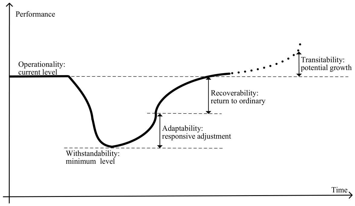
Figure 1. Systematically visualized five dimensions of logistics resilience.
Sustainability 18 07215 g001
Figure 2. The standard deviational ellipse and centroid trajectory.
Sustainability 18 07215 g002
Figure 3. The major axis, minor axis, and flattening ratio.
Sustainability 18 07215 g003
Figure 4. The spatial distribution and correlation structure of logistics resilience.
Sustainability 18 07215 g004aSustainability 18 07215 g004b
Figure 5. The spatial correlation intensity and direction of logistics resilience.
Sustainability 18 07215 g005
Figure 6. The out-degree and in-degree of each province in 2024.
Sustainability 18 07215 g006
Figure 7. The inter-block spillover relationships of logistics resilience in 2013 and 2024.
Sustainability 18 07215 g007
Table 1. Nomenclature of key symbols and definitions.
SymbolDefinition
Part 1: Indicator system and weighting
i , u , h province identifier
j , k , v indicator identifier
t year identifier
x i j t raw value of indicator j for province i in year t
x i j t standardized value of indicator j for province i in year t
m total number of provinces
n total number of indicators
T total number of study period
I C j information content of indicator j
x ¯ j mean value of indicator j
σ j standard deviation of indicator j
C C j conflict coefficient between indicator j and all other indicators
r j k Pearson correlation coefficient of indicator j and k
w j C R I T I C CRITIC weight of indicator j
I U j information utility value of indicator j
I E j information entropy of indicator j
p i j t the proportion of standardized sample of indicator j of province i in year t covering all provinces across the study period
w j e t r o p y improved entropy weight of indicator j
W 1 CRITIC weight vector
W 2 improved entropy weight vector
2 Euclidean 2-norm
α 1 distribution coefficient of CRITIC weight vector
α 2 distribution coefficient of improved entropy weight vector
Part 2: Standard deviation ellipse and centroid migration model
( x i , y i ) geographic coordinates, longitude and latitude, respectively
( X ¯ , Y ¯ ) centroid coordinate
θ azimuth angle
a = σ x major axis standard deviation
b = σ y minor axis standard deviation
x ˜ i = x i X ¯ x-coordinate deviations of province i from the ellipse centroid
y ˜ i = y i Y ¯ y-coordinate deviations of province i from the ellipse centroid
w i spatial weight of province i characterized by its logistics resilience
f flattening ratio
S E ellipse area
Part 3: Modified gravity model and gravity matrix
F i u spatial correlation intensity between province i and u
P i ,   P u regional population in province i and u
L R i ,   L R u regional logistics resilience level of province i and u
G i ,   G u regional GDP of province i and u
d i u geographic distance
g i ,   g u the gap of per capita GDP of provinces i and u
Part 4: Social network analysis
N D network density
A number of actual relationships within the network
N C network connectedness
V number of unreachable nodes
N H network hierarchy
N E network efficiency
K number of symmetrically reachable member pairs
M number of redundant lines
D R degree centrality
C L closeness centrality
r i number of direct relationships correlated to province i
B R betweenness centrality
G L u h ( i ) probability that province i lies on the geodesic between u and h
l u h ( i ) number of geodesics between u and h that include province i
l u h ( t o t a l ) the total number of geodesics between u and h
q block identifier
t q number of provincial nodes in block q
Part 5: QAP model
L R dependent variable matrix composed of the logistics resilience values of each province in the NWLSC
X independent variable matrix corresponding to the driving factors
E random disturbance term
β 0 constant term
β influence coefficient vector to be estimated via regression
Table 2. Typical dimension classifications in the existing literature.
Number of DimensionsTypical LiteratureDimension Names
ThreeZhang et al. [8]Resistance and Recovery Capacity, Adaptation and Adjustment Capacity, Innovation and Transformation Capacity
FourZhang et al. [15]Logistics Supply, Logistics Demand, Industrial Structure, Impact on Environment
FiveLiang et al. [1]Economic Resilience, Shock Absorption, Operational Recovery, Network Load Capacity, Innovation Potential
Table 3. Indicator system for evaluating logistics resilience.
DimensionsIndicatorsQuantified CharacterizationUnitsWeights
Operationalityeconomic contributionadded value of logistics/regional GDP%0.021
expansion from supply chaine-commerce sales and procurement100 M yuan0.069
employment ratio in logisticsemployees in logistics/total employees%0.028
logistics industrial entitieslegal entities in logistics/total legal entities%0.026
real investment in logisticsfixed asset investment in logistics100 M yuan0.059
Withstandabilityoutput scale of logisticsadded value of logistics industry100 M yuan0.041
employment scale of logisticsnumber of employees in logistics10 k persons0.035
scale of transport vehiclestonnage of operating truckstons0.043
transport route densitytransportation route length/areakm/km20.048
postal collaborative servicepostal service outlets/areasites/104 km20.065
Adaptabilityconsumption boostconsumption per capitayuan0.018
income supportdisposable income per capitayuan0.023
economic growthGDP growth rate%0.019
population agglomerationpopulation/areapersons/km20.055
industrial driving effectinventory of industrial enterprises100 M yuan0.041
transportation constructionfiscal transportation expenditure/fiscal budget%0.029
Recoverabilitystatus of freight transporttotal freight volume10 kt0.026
status of express deliverytotal express delivery volume10 k pieces0.010
status of freight turnovertotal freight turnover108 t·km0.010
pressure on freight routesfreight volume/route lengtht/104 km0.025
pressure on express routesexpress delivery volume/route lengthpcs/104 km0.010
Transitabilityindustrial upgradingshare of the tertiary industry%0.016
digital infrastructurelength of optical cable lines/areakm/104 km20.059
social R & DR & D funds/regional GDP%0.033
technology applicationtransaction value of technology market100 M yuan0.143
education investmentfiscal education expenditure/fiscal budget%0.024
human resources cultivationenrolled college students per 100,000 residentspersons0.024
Table 4. Criteria for block clustering.
Proportion of Internal RelationshipCount of Received Internal Block Relationship
>0≈0
1 4 q = 1 4 t q 1 m 1 Net Beneficiary BlockBidirectional Spillover Block
< 1 4 q = 1 4 t q 1 m 1 Broker BlockNet Spillover Block
Table 5. The level of logistics resilience.
RegionsProvinces201320142015201620172018201920202021202220232024MeanGrowth Rate
Main ChannelChongqing0.3510.3650.3900.4130.4390.4530.4850.5210.5290.6050.5900.6300.4815.46%
Sichuan0.2920.3140.3460.3610.3920.4320.4660.4990.5370.5710.5920.6370.4537.34%
Guizhou0.2360.2390.2690.2730.2970.3140.3220.3240.3540.3720.3850.4070.3165.07%
Core AreaGuangxi0.2490.2510.2710.2800.2960.3090.3310.3630.4090.4110.4190.4280.3355.05%
Hainan0.2430.2410.2680.2760.2890.3000.3040.3230.3250.3260.3490.3770.3024.09%
Yunnan0.2390.2370.2610.2680.2980.3120.3380.3270.3620.3670.3570.3670.3113.98%
Xizang0.1220.1260.1370.1310.1400.1540.1820.1560.1750.1720.1840.1840.1553.79%
Extended BeltInner Mongolia0.2440.2370.2470.2550.2560.2560.2740.2810.2750.2950.3150.2960.2691.79%
Shaanxi0.3100.3210.3390.3510.3790.3930.4330.4370.4850.5200.5550.6260.4296.60%
Gansu0.2130.2070.2180.2320.2340.2410.2570.2340.2590.2680.2640.2910.2432.90%
Qinghai0.1740.1630.1740.1800.1790.1820.1930.1740.2000.2020.1890.2000.1841.29%
Ningxia0.2020.2130.2190.2270.2350.2410.2600.2440.2700.2800.2750.2940.2473.47%
Xinjiang0.2110.2190.2290.2240.2360.2450.2640.2440.2800.2870.2940.3270.2554.03%
Mean0.2370.2410.2590.2670.2820.2950.3160.3170.3430.3600.3670.3900.3064.61%
Table 6. Gini coefficient decomposition of overall disparities.
YearTotal GiniIntra-Regional GiniInter-Regional GiniTransvariation Density
20130.1290.03527.36%0.06247.67%0.03224.96%
20140.1380.03726.89%0.07050.56%0.03122.55%
20150.1430.03625.29%0.06948.62%0.03726.08%
20160.1490.03825.09%0.07449.49%0.03825.42%
20170.1590.03824.21%0.07848.98%0.04326.82%
20180.1630.03722.97%0.08753.13%0.03923.89%
20190.1610.03924.14%0.08351.45%0.03924.41%
20200.1940.04623.86%0.10554.28%0.04221.86%
20210.1860.04524.13%0.09752.25%0.04423.62%
20220.2000.04823.83%0.10452.11%0.04824.05%
20230.2020.05124.99%0.10250.51%0.05024.49%
20240.2090.05224.99%0.10047.75%0.05727.26%
mean0.1690.04224.81%0.08650.57%0.04224.62%
Table 7. Parameters of the standard deviational ellipse.
YearCentroid CoordinatesArea
(104 km2)
Major Axis (km)Minor Axis (km)Azimuth Angle (º)Flattening Ratio
Longitude (E)Latitude (N)
2013104°11′04.20″32°00′54.74″315.5811231.325815.862151.8360.337
2017104°17′46.21″31°43′17.41″301.0681210.417791.787151.7940.346
2021104°17′38.17″31°32′17.32″290.0261191.091775.123150.5490.349
2024104°24′29.99″31°35′55.85″284.7281185.786764.368150.0710.355
Table 8. Overall structure and evolutionary characteristics of the spatial correlation network.
YearNetwork DensityNetwork
Relationship
Network
Connectedness
Network HierarchyNetwork Efficiency
20130.3335210.4000.576
20140.3275110.4000.591
20150.3215010.2860.606
20160.3014710.2860.636
20170.3084810.4000.606
20180.3144910.4000.621
20190.3275110.4000.606
20200.2894510.4000.652
20210.3084810.5000.606
20220.3215010.5000.606
20230.3275110.4000.606
20240.3405310.4000.576
Mean0.31849.58310.3980.607
Table 9. Individual nodal functional statuses of the spatial correlation network.
ProvincesDegree CentralityCloseness CentralityBetweenness Centrality
201320172021202420132017202120242013201720212024
Chongqing75.00091.66791.66783.33380.00092.30892.30885.7146.3016.5665.5563.371
Sichuan58.33358.33350.00066.66770.58870.58866.66775.0001.9572.4492.0083.586
Guizhou75.00041.66750.00050.00080.00063.15866.66766.6675.3164.0913.4604.116
Guangxi41.66733.33350.00058.33363.15860.00066.66770.58811.1874.0914.09112.449
Hainan33.33325.00025.00025.00060.00057.14357.14354.5450.5680.0000.0000.189
Yunnan50.00033.33333.33341.66766.66760.00060.00063.1581.7170.3030.0000.000
Xizang41.66741.66733.33341.66763.15863.15860.00063.1580.0000.0000.0000.000
Inner Mongolia66.66775.00066.66775.00075.00080.00075.00080.0005.24011.61611.86914.167
Shaanxi66.66775.00075.00066.66775.00080.00080.00075.00024.41926.76822.34818.876
Gansu58.33366.66766.66766.66770.58875.00075.00075.00016.98228.20720.82120.215
Qinghai33.33333.33333.33341.66760.00060.00060.00063.1580.0000.0000.0000.000
Ningxia41.66733.33333.33333.33363.15860.00060.00060.0000.0000.0000.3030.303
Xinjiang25.00025.00025.00016.66757.14357.14357.14352.1740.5560.0000.0000.000
Mean51.28248.71848.71851.28268.03567.57767.43068.0125.7116.4695.4205.944
Bold = above mean.
Table 10. Block clustering of the spatial network.
YearBlocksProvincesReceived RelationsSpilled RelationsIntra-Block RelationsExpected Internal RatioActual Internal RatioBlock Type
2013Block IXinjiang, Inner Mongolia, Shaanxi1412016.67%0.00%Broker
Block IIHainan, Chongqing9618.33%14.29%Net Beneficiary
Block IIIGuangxi, Guizhou, Yunnan, Sichuan189525.00%35.71%Net Beneficiary
Block IVNingxia, Gansu, Qinghai, Xizang317225.00%10.53%Net Spillover
2017Block IChongqing, Inner Mongolia, Shaanxi2312116.67%7.69%Broker
Block IIHainan, Sichuan6608.33%0.00%Broker
Block IIIGuangxi, Guizhou, Yunnan107016.67%0.00%Broker
Block IVNingxia, Gansu, Qinghai, Xizang, Xinjiang216633.33%27.27%Net Spillover
2021Block IInner Mongolia, Gansu9828.33%20.00%Bidirectional Spillover
Block IINingxia, Qinghai, Xizang, Xinjiang215025.00%0.00%Net Spillover
Block IIIGuangxi, Guizhou, Sichuan146216.67%25.00%Net Beneficiary
Block IVHainan, Chongqing, Shaanxi, Yunnan1511425.00%26.67%Net Beneficiary
2024Block IInner Mongolia, Xinjiang6618.33%14.29%Bidirectional Spillover
Block IINingxia, Qinghai, Xizang, Gansu, Yunnan421333.33%12.50%Net Spillover
Block IIIGuangxi, Guizhou13708.33%0.00%Broker
Block IVHainan, Chongqing, Shaanxi, Sichuan209625.00%40.00%Net Beneficiary
Table 11. Density matrices and corresponding image matrices of the spatial correlation network.
YearBlock TypeDensity MatrixImage Matrix
Block IBlock IIBlock IIIBlock IVBlock IBlock IIBlock IIIBlock IV
2013Block I0.0000.0000.7500.2500010
Block II0.0000.5000.7500.0000110
Block III0.3330.6250.4170.0000110
Block IV0.8330.5000.1880.1671100
2017Block I0.1670.5000.7780.1330110
Block II0.5000.0000.5000.0001010
Block III0.6670.1670.0000.0001000
Block IV0.9330.2000.0000.3001000
2021Block I1.0000.2500.6670.2501010
Block II1.0000.0000.0000.4381001
Block III0.0000.0000.3330.5000011
Block IV0.1250.0000.8330.3330011
2024Block I0.5000.3000.5000.1251010
Block II0.6000.1500.3000.6001001
Block III0.0000.0000.0000.8750001
Block IV0.0000.0501.0000.5000011
Table 12. Results of QAP correlation analysis.
Driving FactorsCorrelation CoefficientSignificance Level
Economic development X10.555 ***0.001
Inclusive finance X20.0320.430
Environmental pollution governance X30.0240.469
Educational advancement X40.292 ***0.007
Industrial structure rationalization X5−0.0110.515
Urbanization level X60.207 *0.056
Technological innovation X70.207 **0.047
Informatization level X8−0.0450.393
Geospatial proximity X90.218 **0.015
*, **, and *** denote 10%, 5%, and 1% statistical significance, respectively.
Table 13. Results of QAP regression analysis.
Driving FactorsNon-Standardized Regression CoefficientStandardized Regression CoefficientSignificance Level
Economic development X10.4920.523 ***0.001
Inclusive finance X2−0.046−0.0490.249
Environmental pollution governance X30.0110.0120.440
Educational advancement X40.1390.150 **0.035
Industrial structure rationalization X50.0120.0130.439
Urbanization level X60.0100.0100.465
Technological innovation X70.0830.0880.132
Informatization level X80.0520.0550.238
Geospatial proximity X90.2990.299 ***0.001
R2 = 0.416, Adjusted R2 = 0.384
** and *** denote 5% and 1% statistical significance, respectively.
Table 14. The level of logistics resilience with the distribution coefficients (0.3, 0.7).
Provinces201320142015201620172018201920202021202220232024MeanGrowth Rate
Chongqing0.3670.3780.4040.4250.4500.4620.4940.5290.5320.6080.5920.6310.4895.07%
Sichuan0.3040.3240.3570.3710.4000.4380.4700.5020.5390.5700.5880.6310.4586.86%
Guizhou0.2530.2540.2840.2870.3100.3280.3350.3360.3680.3820.3930.4160.3294.63%
Guangxi0.2630.2650.2850.2930.3080.3210.3420.3740.4140.4170.4270.4340.3454.64%
Hainan0.2620.2590.2870.2930.3060.3180.3220.3400.3400.3390.3620.3900.3183.68%
Yunnan0.2550.2500.2750.2820.3110.3250.3520.3380.3740.3790.3670.3770.3243.61%
Xizang0.1420.1450.1560.1490.1590.1740.2050.1760.1960.1920.2060.2050.1753.43%
Inner Mongolia0.2610.2520.2640.2720.2710.2710.2900.2970.2880.3080.3300.3080.2841.50%
Shaanxi0.3240.3330.3510.3620.3910.4030.4420.4430.4900.5210.5510.6200.4366.08%
Gansu0.2310.2230.2340.2500.2520.2590.2760.2500.2760.2850.2790.3070.2602.62%
Qinghai0.1950.1820.1940.2010.1990.2020.2140.1920.2200.2220.2080.2210.2041.15%
Ningxia0.2200.2320.2380.2460.2540.2590.2800.2610.2890.2990.2920.3110.2653.19%
Xinjiang0.2300.2370.2480.2430.2550.2630.2850.2610.3000.3050.3100.3430.2733.68%
Mean0.2540.2560.2750.2820.2970.3090.3310.3310.3560.3710.3770.3990.3204.19%
Table 15. The level of logistics resilience with the distribution coefficients (0.4, 0.6).
Provinces201320142015201620172018201920202021202220232024MeanGrowth Rate
Chongqing0.3840.3930.4190.4380.4630.4730.5040.5380.5370.6120.5940.6330.4994.64%
Sichuan0.3180.3360.3710.3820.4090.4450.4740.5060.5420.5700.5840.6240.4636.32%
Guizhou0.2720.2710.3020.3020.3260.3430.3500.3490.3840.3950.4030.4260.3444.18%
Guangxi0.2800.2800.3010.3080.3220.3350.3550.3860.4200.4250.4360.4410.3574.21%
Hainan0.2840.2790.3070.3130.3270.3390.3420.3610.3570.3540.3780.4040.3373.26%
Yunnan0.2740.2650.2920.2980.3270.3400.3680.3500.3880.3930.3780.3890.3393.23%
Xizang0.1640.1660.1790.1700.1800.1970.2300.1990.2210.2160.2310.2300.1983.11%
Inner Mongolia0.2800.2700.2830.2900.2890.2890.3090.3150.3030.3240.3470.3200.3021.21%
Shaanxi0.3400.3460.3650.3730.4040.4140.4530.4490.4960.5230.5460.6130.4445.50%
Gansu0.2520.2420.2540.2710.2720.2790.2980.2680.2960.3040.2970.3260.2802.35%
Qinghai0.2180.2030.2170.2240.2220.2250.2390.2140.2440.2450.2300.2440.2271.02%
Ningxia0.2420.2540.2590.2670.2750.2810.3030.2810.3110.3200.3120.3320.2862.92%
Xinjiang0.2520.2590.2700.2650.2760.2850.3080.2810.3220.3260.3280.3620.2953.34%
Mean0.2740.2740.2940.3000.3150.3270.3490.3460.3710.3850.3900.4110.3363.76%
Table 16. The level of logistics resilience with the distribution coefficients (0.5, 0.5).
Provinces201320142015201620172018201920202021202220232024MeanGrowth Rate
Chongqing0.4020.4080.4350.4520.4760.4830.5140.5470.5410.6150.5970.6340.5094.23%
Sichuan0.3320.3470.3840.3940.4180.4520.4790.5110.5440.5690.5790.6170.4695.81%
Guizhou0.2910.2880.3200.3180.3420.3590.3650.3630.3990.4070.4140.4370.3593.77%
Guangxi0.2970.2960.3160.3220.3370.3490.3670.3980.4260.4320.4450.4480.3693.81%
Hainan0.3060.2990.3280.3340.3470.3600.3630.3810.3750.3690.3940.4190.3562.89%
Yunnan0.2930.2800.3090.3150.3420.3560.3840.3630.4030.4070.3900.4000.3532.88%
Xizang0.1860.1880.2010.1900.2010.2200.2560.2220.2460.2390.2560.2540.2222.86%
Inner Mongolia0.3000.2880.3020.3090.3060.3070.3270.3330.3180.3390.3640.3330.3190.95%
Shaanxi0.3560.3600.3790.3850.4170.4260.4640.4550.5020.5250.5420.6060.4514.95%
Gansu0.2730.2600.2730.2920.2920.3000.3200.2860.3160.3240.3140.3440.3002.11%
Qinghai0.2420.2240.2400.2470.2450.2480.2640.2350.2680.2690.2520.2670.2500.91%
Ningxia0.2640.2760.2810.2890.2970.3020.3260.3010.3330.3410.3310.3530.3082.68%
Xinjiang0.2740.2810.2920.2880.2980.3060.3320.3010.3440.3470.3460.3810.3163.04%
Mean0.2930.2920.3120.3180.3320.3440.3660.3610.3860.3990.4020.4230.3523.37%
Table 17. Overall structure characteristics of the spatial correlation network with a binarization threshold of the 65th quantile.
YearNetwork DensityNetwork
Relationship
Network
Connectedness
Network HierarchyNetwork Efficiency
20130.3335210.6490.621
20140.3335210.2860.621
20150.3335210.4000.606
20160.3335210.5000.576
20170.3335210.5000.576
20180.3335210.5000.591
20190.3335210.5000.591
20200.3335210.4000.606
20210.3335210.5000.576
20220.3335210.4000.606
20230.3335210.4000.606
20240.3335210.4000.591
Mean0.3335210.4530.597
Table 18. Individual nodal functional statuses of the spatial correlation network with a binarization threshold of the 65th quantile.
ProvincesDegree CentralityCloseness CentralityBetweenness Centrality
201320172021202420132017202120242013201720212024
Chongqing66.66791.66791.66791.66775.00092.30892.30892.3085.80814.20613.63613.826
Sichuan41.66758.33350.00050.00063.15870.58866.66766.6671.7685.0401.8941.894
Guizhou75.00041.66750.00041.66780.00063.15866.66763.1585.9343.7417.5767.008
Guangxi41.66741.66750.00058.33363.15863.15866.66770.5889.3439.7739.84810.922
Hainan33.33333.33333.33333.33360.00060.00060.00060.0000.2530.9361.7052.462
Yunnan50.00041.66733.33333.33366.66763.15860.00060.0001.6411.8580.1891.326
Xizang33.33333.33333.33333.33360.00060.00060.00060.0000.7580.0000.0000.000
Inner Mongolia58.33375.00075.00083.33370.58880.00080.00085.7144.0406.69210.22715.909
Shaanxi66.66783.33383.33366.66775.00085.71485.71475.0007.0716.7375.1144.040
Gansu50.00066.66766.66758.33366.66775.00075.00070.5886.0611.7751.3269.659
Qinghai33.33333.33333.33333.33360.00060.00060.00060.0000.0000.0000.0000.000
Ningxia33.33333.33333.33333.33360.00060.00060.00060.0000.0000.0000.0000.000
Xinjiang33.33333.33333.33333.33360.00060.00060.00060.0004.2930.0000.0000.379
Mean47.43651.28251.28250.00066.17268.69968.69468.0023.6133.9043.9635.187
Bold = above mean.
Table 19. Results of QAP correlation analysis excluding 2020 to 2022.
Driving FactorsCorrelation CoefficientSignificance Level
Economic development X10.521 ***0.001
Inclusive finance X20.1320.128
Environmental pollution governance X30.0330.432
Educational advancement X40.288 **0.008
Industrial structure rationalization X50.1090.237
Urbanization level X60.213 **0.040
Technological innovation X70.241 **0.030
Informatization level X8−0.0760.302
Geospatial proximity X90.207 **0.020
** and *** denote 5% and 1% statistical significance, respectively.
Table 20. Results of QAP regression analysis excluding 2020 to 2022.
Driving FactorsNon-Standardized Regression CoefficientStandardized Regression CoefficientSignificance Level
Economic development X10.4650.494 ***0.001
Inclusive finance X20.0240.0260.368
Environmental pollution governance X30.0170.0180.397
Educational advancement X40.0780.0840.183
Industrial structure rationalization X50.0820.0870.159
Urbanization level X60.0590.0630.231
Technological innovation X70.1170.124 *0.072
Informatization level X80.0560.0600.236
Geospatial proximity X90.3000.299 ***0.001
R2 = 0.395, Adjusted R2 = 0.362
* and *** denote 10% and 1% statistical significance, respectively.
Table 21. Results of QAP analysis when removing insignificant variables.
Driving FactorsCorrelation CoefficientSignificance LevelStandardized Regression CoefficientSignificance Level
Economic development X10.555 ***0.0010.518 ***0.001
Educational advancement X40.292 ***0.0090.137 *0.050
Urbanization level X60.207 ***0.0600.0110.457
Technological innovation X70.207 ***0.0470.0810.146
Geospatial proximity X90.218 **0.0130.293 ***0.001
R2 = 0.411, Adjusted R2 = 0.395
*, **, and *** denote 10%, 5%, and 1% statistical significance, respectively.
Table 22. Results of QAP analysis when adding government intervention to the previous six variables.
Driving FactorsCorrelation CoefficientSignificance LevelStandardized Regression CoefficientSignificance Level
Economic development X10.555 ***0.0010.517 ***0.001
Educational advancement X40.292 ***0.0100.136 *0.053
Urbanization level X60.207 **0.0580.0110.446
Technological innovation X70.207 **0.0500.0810.152
Geospatial proximity X90.218 **0.0140.293 ***0.001
Government intervention X10−0.1630.102−0.0030.483
R2 = 0.405, Adjusted R2 = 0.393
*, **, and *** denote 10%, 5%, and 1% statistical significance, respectively.
Table 23. Results of QAP analysis when adding government intervention to the previous nine variables.
Driving FactorsCorrelation CoefficientSignificance LevelStandardized Regression CoefficientSignificance Level
Economic development X10.555 ***0.0010.522 ***0.001
Inclusive finance X20.0320.430−0.0490.261
Environmental pollution governance X30.0240.4690.0120.449
Educational advancement X40.292 ***0.0070.149 **0.033
Industrial structure rationalization X5−0.0110.5150.0130.429
Urbanization level X60.207 *0.0560.0100.444
Technological innovation X70.207 **0.0470.0880.140
Informatization level X8−0.0450.3930.0550.250
Geospatial proximity X90.218 **0.0150.299 ***0.001
Government intervention X10−0.1630.101−0.0020.488
R2 = 0.416, Adjusted R2 = 0.380
*, **, and *** denote 10%, 5%, and 1% statistical significance, respectively.
Disclaimer/Publisher’s Note: The statements, opinions and data contained in all publications are solely those of the individual author(s) and contributor(s) and not of MDPI and/or the editor(s). MDPI and/or the editor(s) disclaim responsibility for any injury to people or property resulting from any ideas, methods, instructions or products referred to in the content.