Parameterisation of Rural Built-Up Areas for Analysing the Determinants of Land Consolidation Constraints

Abstract

The characteristics of existing rural built-up areas may influence the scope and nature of land consolidation and agricultural land management. Built-up areas delineate the boundaries of current and potential agricultural land, determine the spatial structure of farms, and constitute major components of the local landscape. It may be assumed that a precise mathematical description of rural built-up areas would provide valuable information in the context of rural studies, including the comparative analyses of villages presented in this study and the development of predictive models aimed at assessing the difficulty of land consolidation. However, the complete implementation of this task has not yet been reported in the scientific literature. The aim of this study was to develop a methodology for the mathematical description of rural built-up areas, with particular emphasis on factors potentially influencing the difficulty of land consolidation. Based on an in-depth review of the scientific and technical literature, nine diverse and partially interrelated indicators were identified, and a precise method for their calculation was defined in this study. In addition, a set of scripts and programs was developed and made publicly available to automate the calculations, thereby enabling their application in future research. The obtained results enabled an objective and unambiguous description of villages, which is essential for research on the relationship between the structure of rural built-up areas and the difficulty of land consolidation in Poland.

1. Introduction

Research on the optimisation of land consolidation methodology, aimed at increasing the efficiency of design solutions [1,2,3,4,5,6,7] and implementing works in a comprehensive manner in line with the concept of sustainable rural development [8,9], is regularly conducted by researchers mainly from European [10,11,12,13,14,15,16], Asian [16,17], and African countries [18]. The existing body of international literature presents advanced concepts and technical solutions, including in the field of automated design of post-consolidation farm layouts [19], multi-criteria assessment and prioritisation of land consolidation urgency [20,21,22,23], evaluation of completed consolidation projects and monitoring of their long-term effects [24], and assessment of their impact on the natural environment [25], local landscape values [26], and the economic performance of farms [27,28].

The considerable number of published studies on land consolidation and their thematic diversity correspond to the significance of this research area. Land consolidation, as a fundamental land management and agricultural engineering measure [29], enables the correction of defective spatial structures of farms shaped over decades by various social and political factors [30]. Comprehensive land consolidation projects that consider social [31,32], landscape [33], and environmental aspects [34,35,36] enable the sustainable modernisation of rural areas, aimed at improving living conditions and stimulating sustainable socio-economic development [30,33].

Despite the considerable number of studies devoted to land consolidation, examples of which have been cited above, there are still areas in the current scientific literature that remain unexplored or are described only in general terms, providing insufficient theoretical knowledge and limited practical applicability of the findings. According to the authors, one such area is the comprehensive technical assessment of the difficulty of land consolidation. The international literature contains isolated references suggesting the importance of considering land consolidation difficulties in planning and implementing processes [37]. Some publications include terrain difficulty as one of the elements of the general assessment of land consolidation priority [22]; however, none of the available studies provides a coherent and objective method that enables detailed or comparative research on land consolidation difficulty.

This research addresses the identified gap in the objective parameterisation of rural areas. While the studies are primarily conducted in the Subcarpathian Voivodeship (southeastern Poland), the methodology is designed for broad applicability and can be implemented in other regions following appropriate adaptation. This work builds upon a multistage research programme regarding the technical difficulty of land consolidation, which commenced in 2024 with a study focused on cadastral data analysis [12]. Another research stage concerns the development of a methodology for assessing land consolidation difficulty in relation to the characteristics of rural built-up areas. The research presented in this paper provides a complete and standalone conceptual framework for the parameterisation of rural built-up areas. It introduces a novel set of mathematical indicators and automated tools that offer an independent solution for rural spatial analysis. By establishing this objective methodology, the paper provides a foundational framework for analysing the relationship between settlement characteristics and land consolidation difficulty, ultimately enabling the development of advanced predictive models.

The research activities included a review of scientific and technical literature regarding available methods for parameterising rural built-up areas, the development of an original set of parameters of a built-up area together with corresponding formulas and computational algorithms, the creation of automated computational tools for indicator calculation based on building geometry, and experimental implementation of the developed tools for a study sample comprising 40 villages located in the Subcarpathian Voivodeship (southeastern Poland).

The result of this study is a detailed conceptual framework for the parameterisation of rural built-up areas with a set of tools enabling its implementation in an open QGIS environment. The developed scripts and programs have been made publicly available in a GitHub repository (commit: f2728eb), ensuring full reproducibility of the research and enabling immediate application in rural studies and planning tasks. The acquired theoretical knowledge and functional tools have also enabled further stages of the research to be undertaken, which are expected to be published in future articles.

2. Literature Review

Although no comprehensive approaches to the parameterisation of rural built-up areas applicable to land consolidation have been identified in the current scientific and technical literature, several studies partially related to the objectives of this research can be found in the international literature. The following literature review serves as the theoretical basis for the subsequent selection of built-up area parameters. The analysis was divided into two stages. The first (Section 2.1) is a general review of rural studies literature with respect to mathematical descriptions of parameters of rural built-up areas. The second stage (Section 2.2) covers an analysis of selected technical documents concerning land consolidation planning and implementation in Poland, with a particular focus on indications regarding the influence of the built-up area structure or its components on land consolidation.

2.1. Review of Rural Studies Literature

Traditional and widely cited concepts for the classification and description of rural built-up areas in the literature typically attempt to relate the geometric form of settlement structures to their presumed genesis. The foundations of this classification for Polish territories were described by Zaborski [38], who referred to the research work of Meitzen [39]. Despite the considerable time that has passed, the assumptions underlying this concept remain valid in the view of successive generations of researchers [40,41,42]. The proposed classification distinguishes morphogenetic types of villages, such as circular, ring-shaped, oval, single-street, multi-road, etc. [38]. A similar but simplified classification method was proposed by Myga-Piątek [43], who distinguished compact and dispersed settlements, as well as geometric and irregular forms, and by Szymańska [44], who suggested a division of settlement forms into clustered and dispersed types.

While the aforementioned classification of rural settlement structures is well established in both historical and contemporary rural studies, underscoring its scientific importance, it has limited applicability in assessing the technical difficulty of land consolidation. First, the authors classified villages based on their characteristic features and historical conditions. The application of a similar approach to the description of potential consolidation objects would be time-consuming, and the resulting classification would largely depend on the subjective interpretation of experts. Second, the use of a nominal scale limits the possibilities for statistical analysis and the development of automated computational tools.

Alternative concepts for describing rural built-up areas identified in Polish scientific literature are based on quantitative indicators. Szymańska [44] proposes two basic criteria for the classification of settlements: form, understood as the “geometric shape and layout of settlements”, which may be described using parameters such as “length, linearity, built-up pattern and L-shape”, or simplified settlement dimensions (length and width), and type, characterised by the “relationship between the number of houses, farmsteads and their mutual distances”. However, the author does not provide mathematical formulas for the unambiguous calculation of these characteristics, which constrains the possibility of their evaluation and practical application in the subject study.

Gibas and Heffner [45] present a concept for the mathematical description of building concentration as the mean distance between address points within the analysed area. Sudra [46] proposed a complex description of spatial building concentration, including parameters such as the Gini coefficient of cumulative concentration, Kostrubiec concentration index, nearest-neighbour distance method, Clark-Evans index, and Shannon entropy. Serafin [47], in studies concerning areas located at the urban and rural interface, used relatively simple measures, including the density of residential and farm buildings per unit area and the percentage share of built-up area in the total area of the study site, calculated using a formula developed by Śleszyński [48]. Serafin [47] additionally indicated the possibility of disaggregating the total built-up area into categories representing different types of development, such as single-family housing, multi-family housing, compact, loose, and dispersed development. Meanwhile, Salata [49], presenting an original concept for defining built-up areas together with a methodology for their delineation, introduced the percentage indicator of land coverage by built-up areas as one of the measures characterising the settlement unit.

Considering the specificity of the conducted research, it was assumed that the methodology for describing rural built-up areas would be based on quantitative indicators that can be calculated using mathematical formulas and spatial analysis algorithms. Despite the lack of an existing solution enabling an objective characterisation of rural built-up areas in the context of land consolidation, it was assumed that the concepts described above may constitute a substantive basis for developing a new, original set of indicators.

2.2. Review of Technical and Regulatory Literature on Land Consolidation

At this stage of the source analysis, a detailed review was conducted of three documents concerning the technical and legal aspects of land consolidation in Poland.

• Act of 26 March 1982 on Land Consolidation and Exchange [50];
• Instruction No. 1 of the Minister of Agriculture and Food Economy on Land Consolidation and Exchange of 24 March 1983 [51];
• Internal Catalogue of Work Standards of the Subcarpathian Office of Land Surveying and Agricultural Areas in Rzeszów [52].

The first document listed constitutes the fundamental binding legal act regulating land consolidation in Poland. The Act defines, among other things, the legal and organisational aspects of consolidation proceedings with respect to their key stages. However, it does not cover all issues related to the technical aspects of land consolidation, which are significant from the contractor’s perspective. These issues are addressed in the subsequent document cited, namely Instruction No. 1 of the Minister of Agriculture and Food Economy on Land Consolidation and Exchange of 24 March 1983. This document, structured into 12 thematic chapters, defines the sequence and scope of the elementary activities recommended within the consolidation procedure. Despite its considerable obsolescence (partly mitigated by subsequent updates) and lack of legal force [53], the document remains an important source of information on land consolidation procedures for practitioners and researchers [54,55,56,57] and a reference for public administration bodies [58]. The last analysed source is an internal normative catalogue used by the Subcarpathian Office of Land Surveying and Agricultural Areas in Rzeszów, which is authorised to implement land consolidation projects in the Subcarpathian Voivodeship. The document specifies the activities conducted within the consolidation procedure and provides the basis for estimating the expected duration of each task.

Based on the above documents, a list of elementary activities performed within land consolidation was compiled, the difficulty of which may depend on the characteristics of rural built-up areas. The resulting list is shown in

Table 1. List of activities whose difficulty is assessed as dependent on the characteristics of rural built-up areas: Source: [59] based on: [50,51,52].

No.	Activity	Source
1.	Establishment, stabilisation, and measurement of the control survey network (optional)	[51] (§ 32(1)); [52] (standard 8)
2.	Determination, stabilisation, and measurement of the external boundaries of the consolidation area	[50] (Art. 7a(1)); [51] (§ 32(2)); [52] (standard 2)
3.	Development of the general land consolidation design (design of land complexes)	[51] (§§ 33–38); [52] (standard 7)
4.	Surveying of invariant elements of consolidation designs, such as parcel boundaries in built-up and forest areas	[51] (§ 57(2)); [52] (standard 2)
5.	Supplementary building surveys	[52] (standard 2)
6.	Preparation of the preliminary design (“layout”), including the arrangement of designed parcels within land complexes and sub-complexes	[51] (§ 57(2)); [52] (standard 9)
7.	Setting out and stabilisation of the consolidation design in the field	[50] (Art. 23(2)); [51] (§§ 76–82); [52] (standard 14)
8.	Internal verification of the land consolidation design	[51] (§ 83)
9.	Amendments to the consolidation design following the examination of objections (all desk research and field work)	[50] (Art. 26); [52] (standard 17)

.

The above list includes activities that are directly influenced by the characteristics of rural built-up areas (such as building surveys and built-up zones) and indirectly affected tasks (including selected fields and design works). Building density and spatial distribution may influence the time consumption of surveying work, mobility of surveying teams, and efficiency of farm layout design.

The Internal Catalogue of Work Standards of the Subcarpathian Office of Land Surveying and Agricultural Areas in Rzeszów also includes mathematical formulas for calculating normative working time, considering a terrain difficulty coefficient defined on the basis of a point-based scale covering categories such as topography, visibility, accessibility, and building development. The building development category adopts a three-level scoring scale, where a higher score corresponds to greater terrain difficulty: scattered hamlet-type development, 0 points; single-street type, 2 points; and multi-street type, 6 points. According to the assumptions of the document, the assessment was performed by an authorised expert committee [52].

The availability of the above information indicates the potential usefulness of the document in the context of assessing land consolidation difficulties. However, its scientific value is limited by the lack of empirical validation of the adopted scoring scale in the literature. The classification of building development based on expert judgement may also fail to ensure sufficient objectivity in the assessment. Moreover, the proposed methodology assumes the use of a nominal scale (cf. Section 2.1), followed by an arbitrary interpretation of this scale as an ordinal scale with assigned numerical values without the application of a precise mathematical model. This approach leads to multiple levels of data generalisation, negatively affecting the reliability of the obtained results.

In light of the conducted analysis and critical review of the literature, it was assumed that an effective tool for estimating land consolidation difficulty in relation to rural built-up areas should be based on quantitative characteristics derived using an objective (mathematical) approach. A detailed description of the selected indicators and proposed methodology for their calculation is presented in Section 3.

3. Materials and Methods

3.1. Source Data

The primary data source used for calculating the characteristics of rural built-up areas consisted of vector and georeferenced representations of building outlines in ETRF2000-PL/CS92 coordinate system (EPSG:2180). This study utilised partially generalised objects from the Topographic Object Database at a scale of 1:10,000, which is freely available and covers the territory of Poland. However, a fully functional alternative solution may also involve the use of open global building datasets, such as the Microsoft Global Building Footprints [60] and OpenStreetMap [61]. The use of simple, openly available spatial data ensured the universality of the developed methodology and reduced the complexity and cost of the research. The obtained vector data were pre-validated using native QGIS algorithms to eliminate potential faulty geometries, including duplicates, null geometries, or other topological errors.

3.2. Selection of Indicators

The selection of indicators characterising rural built-up areas was based on a synthesis of information obtained from an analysis of source materials, including scientific publications on rural studies and normative and technical documents regulating the consolidation of agricultural land. The following characteristics of rural built-up areas were identified [59]:

• $g_1$—length of built-up areas;
• $g_2$—elongation of built-up areas;
• $g_3$—surface area of built-up areas;
• $g_4$—number of built-up areas;
• $g_5$—number of buildings;
• $g_6$—average number of buildings per 1 ha of built-up areas;
• $g_7$—average number of buildings per 1 ha of cadastral unit;
• $g_8$—average distance between buildings within a built-up area;
• $g_9$—length of the approximate Hamiltonian cycle for all buildings in a village.

The above indicators describe rural built-up areas in different ways, capturing their size, density, and geometric form using both absolute and relative measures. Although a comprehensive analysis of the relationships between these variables and land consolidation difficulty is reserved for future research, certain expectations can be outlined based on technical literature [50,51,52,59] and practical experience. The potential dependencies between parameters $g_1$–$g_9$ and the stages of a typical land consolidation procedure are summarised in Section 3.4.1, Section 3.4.2, Section 3.4.3, Section 3.4.4, Section 3.4.5, Section 3.4.6, Section 3.4.7, Section 3.4.8 and Section 3.4.9, which also contain the methodological foundations of their calculation.

Owing to the technical similarity between the indicators, it may be assumed that strongly correlated variable pairs will occur within the selected set. However, potentially high correlation coefficients do not exclude the usefulness of variables in assessing land consolidation difficulty. The ultimate mathematical model will be developed by considering appropriate weighting coefficients and the significance of the relationships between individual indicators and the overall measure of land consolidation difficulty.

3.3. Delineation of Built-Up Areas

The indicators $g_1$, $g_2$, $g_3$, $g_4$, $g_6$ and $g_8$ are calculated based on vector, georeferenced boundaries of so-called built-up areas. These objects do not constitute the primary input data for the proposed computational procedure (cf. Section 3.1). Therefore, the application of these indicators requires a consistent mathematical definition of a built-up area and a computational algorithm.

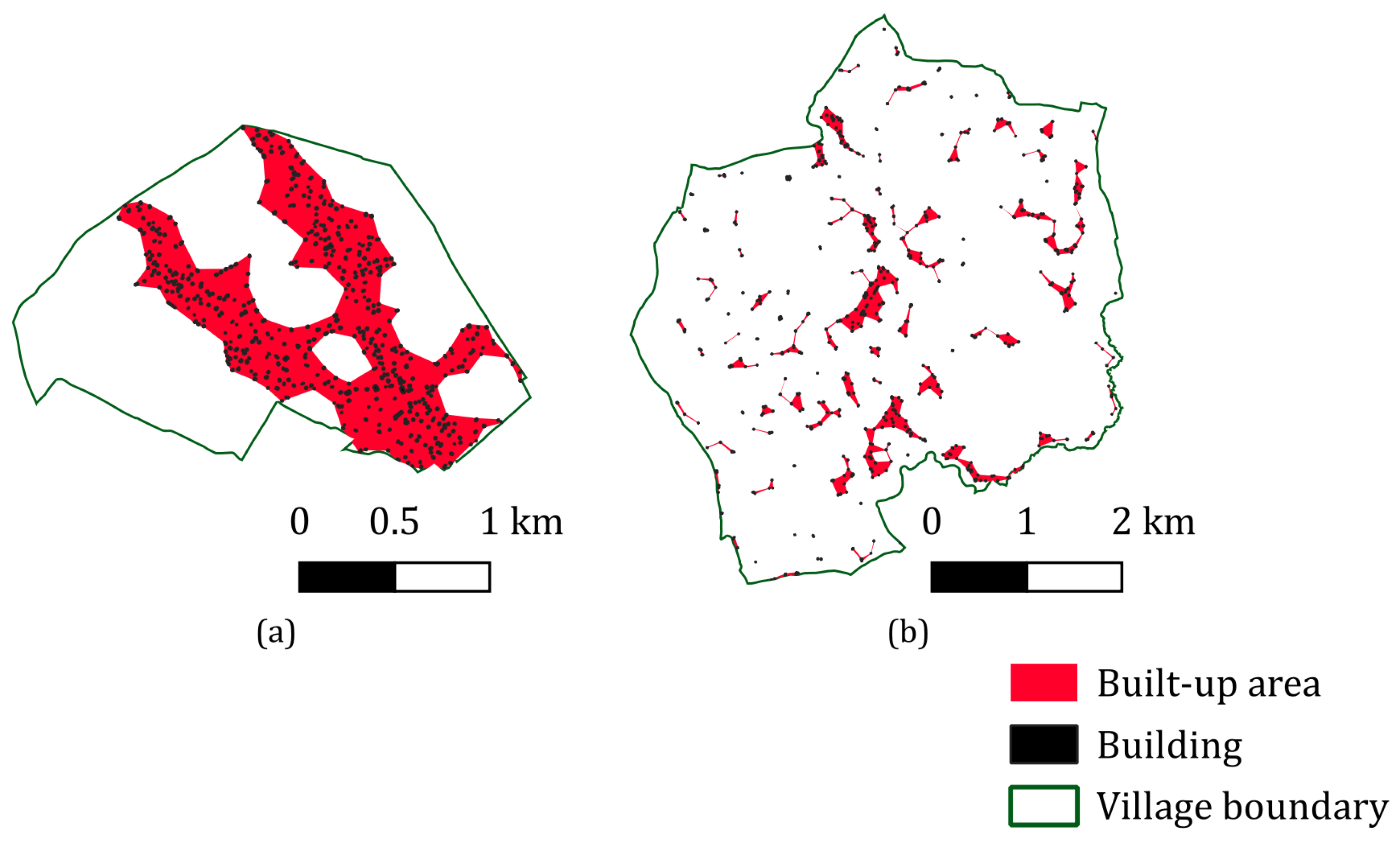
To address this problem, the delineation methodology for built-up areas proposed by Salata is recommended. The author defined a built-up area as a “polygonal object” created through the aggregation of an irregular Delaunay triangulation mesh based on building corners, where none of the triangle edges exceeded 160 m. Triangles in which at least one edge is longer than the specified threshold are not considered part of the built-up area” [49]. In the absence of neighbouring buildings within a maximum distance of 160 m, an isolated building constitutes a separate built-up area. As recommended by the author, this definition was implemented as an algorithm in the QGIS software. For the purposes of this study, a Python 3.12 script was developed to execute the algorithm based on the building outlines. The output of the tool for two villages with different numbers and spatial configurations of built-up areas is presented in Figure 1.

Due to the presence of more than one built-up area in most of the analysed villages, the values of indicators $g_1$, $g_2$, $g_6$ and $g_8$ calculated at the level of built-up areas were aggregated to the village level using a surface-area-weighted mean. The aggregation principle is defined by Equation (1) [59]:

$$v={\displaystyle \frac{{\sum }_i^n{v}_i\ast S_i}{{\sum }_i^n{S}_i}}$$

(1)

where

$v$—value of a specific parameter for the analysed village;

$v_i$—value of a specific parameter for the $i$-th built-up area;

$S_i$—surface area of the $i$-th built-up area;

$n$—number of built-up areas within the analysed village.

3.4. Indicator Calculation Methods

For each indicator, a precise calculation method was defined based on vector objects representing buildings and built-up areas. Each mathematical formula or algorithm was implemented as a Python script operating in QGIS 3.40.0 or as a C++ program. The conceptual schemes, mathematical formulas and QGIS algorithm models and general framework of the scripts/programs were created manually by the authors, whereas the final versions of the software were debugged and optimised using ChatGPT 4o AI model. Subsequently, all developed scripts and programs were validated by the authors using small data samples that had been previously processed manually, following the theoretical formulas and conceptual schemes presented in Section 3.4.1, Section 3.4.2, Section 3.4.3, Section 3.4.4, Section 3.4.5, Section 3.4.6, Section 3.4.7, Section 3.4.8 and Section 3.4.9. The developed computational tools ensure full automation of the calculation process, enabling efficient large-scale studies at the district, regional, or country level. The scripts and programs, together with user documentation, are available in an open GitHub repository [62] under the GNU General Public License v3.0.

3.4.1. Length of Built-Up Areas ($g_1$)

The length of relatively compact built-up areas may influence, among other factors, the flexibility of designing the road network and planning the distribution of farm land in relation to residential and farm buildings. The presence of relatively long rows of buildings, combined with a limited road network, may also constitute a transportation obstacle during the execution of surveying work. Conversely, a linear distribution of buildings may facilitate certain tasks, such as supplementary building surveys and activities requiring the presence of surveying staff at the residences of land consolidation participants [59].

The value of the indicator, expressed in metres, was calculated as the length of the longer edge of the minimum rectangle enclosing a given built-up area. The generation of this rectangular geometry was based on the native algorithm of the QGIS software. The complete computational procedure, including result aggregation, was implemented in the script PAW g1 DŁUGOŚĆ 1.1.py.

3.4.2. Elongation of Built-Up Areas ($g_2$)

Similarly to the parameter of the length of built-up areas ($g_1$), it is hypothesised that linear built-up areas, characterized by significant elongation, may be assessed as favourable for activities involving the mobility of staff in the vicinity of residential and farm buildings (e.g., supplementary building surveys, direct contact with land consolidation participants, etc.). Conversely, such structures may be considered unfavourable in the context of the priority of allocating agricultural land in the proximity of buildings belonging to individual farms. However, this hypothesis requires verification through further detailed research [59].

The elongation of individual built-up areas was calculated using the indicators proposed by Litwin and Szewczyk [63]. The formula was extended to include the handling of cases where the input values fell outside the originally defined domain of the function. The final computational formula for the indicator $g_2$ is given by the following Equation (2) [59]:

$$g_2=\left\{\begin{array}{c}{\displaystyle \frac{L+\sqrt{L^2-16\ast S}}{L-\sqrt{L^2-16\ast S}}}, if L-\sqrt{L^2-16\ast S} \ne 0 and L^2\ge 16\ast S\\ 0, if L-\sqrt{L^2-16\ast S}=0\\ 0, if L^2<16\ast S\end{array}\right.$$

(2)

where:

$L$—perimeter of the plot (built-up area);

S—surface area of the plot (built-up area).

The computational algorithm was implemented in the script PAW g2 WYDŁUŻENIE 1.1.py.

3.4.3. Surface Area of Built-Up Areas ($g_3$)

The surface area of individual built-up areas can serve as an indicator reflecting their significance in the process of designing the spatial structure of farms. Built-up areas with a substantial surface area, typically functioning as the village’s main economic centres, determine elements such as the layout of the road network, among others. Furthermore, the presence of extensive built-up areas significantly influences the technical process of designing land complexes during the project planning stage [59].

The value of the indicator $g_3$ was calculated as the arithmetic mean of the areas of all built-up areas identified within the study area, according to Equation (3) [59]:

$$g_3={\displaystyle \frac{{\sum }_i^n{S}_i}{n}}$$

(3)

where:

$S_i$—surface area of the $i$-th built-up area;

$n$—number of built-up areas within the analysed village.

Automatic computation of this indicator $g_3$ is performed by the script PAW g3 POWIERZCHNIA 1.1.py.

3.4.4. Number of Built-Up Areas ($g_4$)

Built-up areas, functioning as potential invariant elements alongside terrain obstacles, represent one of the primary constraints regarding the design of the spatial structure of farms. A substantial number of built-up areas typically results in the complex geometry of agricultural lands undergoing modification, frequently limiting the potential for optimal farm layout design [59].

The value of the indicator $g_4$ corresponds to the total number of built-up areas identified within the analysed area. Calculations are performed using the script PAW g4 LICZBA OBSZARÓW ZABUDOWY 1.1.py.

3.4.5. Number of Buildings ($g_5$)

The inclusion of the number of buildings in the characterisation of villages was suggested by, among others, Szymańska [44]. The total number of buildings within the consolidation area also constitutes one of the determinants of the volume and complexity of work carried out, particularly during the surveying of invariant elements and supplementary building surveys [51,52,59].

This indicator $g_5$ is calculated as the total number of buildings within the analysed village. It is calculated automatically using the script PAW g5 LICZBA BUDYNKÓW 1.1.py.

3.4.6. Average Number of Buildings per 1 ha of Built-Up Areas ($g_6$)

The building density within individual rural built-up areas may determine the level of difficulty of surveying work and influence the complexity of other technical activities performed during land consolidation. High building density, characteristic of compact development, restricts the mobility of surveying teams and may adversely affect the positioning accuracy of GNSS receivers [59].

This indicator $g_6$, describing the average building density within areas of concentration, is calculated as the ratio of the total number of buildings within the analysed area (village) to the total surface area of the delineated built-up areas, according to Equation (4) [59]:

$$g_6={\displaystyle \frac{l_b}{{\sum }_i^n{S}_i}}$$

(4)

where:

$l_b$—number of buildings in the analysed village;

$n$—number of built-up areas in the analysed village;

$S_i$—surface area of the $\mathrm{i}$-th built-up area.

Automatic calculation of this indicator is possible by using the script PAW g6 GĘSTOŚĆ BUDYNKÓW W OBSZ ZAB 1.2.py.

3.4.7. Average Number of Buildings per 1 ha of Land ($g_7$)

The overall building density of the studied cadastral units was expressed as the average number of buildings per 1 ha of land area. This indicator may partially reflect the potential difficulty of performing design and surveying activities, particularly due to the dual nature of buildings being regarded simultaneously as objects of measurement and terrain obstacles. A significant concentration of buildings within a cadastral unit may preclude the possibility of developing an efficient land consolidation design [59].

This indicator $g_7$ represents the overall building density within the analysed village and is calculated according to Equation (5) [59]:

$$g_7={\displaystyle \frac{l_b}{S}}$$

(5)

where:

$l_b$—number of buildings in the analysed village;

$S$—total surface area of the analysed village.

Values of this indicator are calculated using the script PAW g7 GĘSTOŚĆ BUDYNKÓW W OBR EWID 1.1.py.

3.4.8. Average Distance Between Buildings Within a Built-Up Area ($g_8$)

The average distance between buildings within a built-up area, serving as an indicator of building compactness, represents an adaptation of the parameters for the morphogenetic description of villages proposed by Szymańska [44] and indirectly by Gibas and Heffner [45]. In the context of analysing land consolidation difficulty, this indicator enables a preliminary assessment of potential obstacles regarding the mobility of surveying teams and the execution of surveying work. While compact development may constitute a transportation barrier and an obstacle disrupting GNSS signal propagation, the concentration of buildings within coherent built-up areas allows for a reduction in the time and costs required for surveyors to move between farmsteads during the land consolidation process [59].

This indicator $g_8$, representing the relative compactness of buildings within areas of concentration, is based on the nearest neighbour relationship. It is assumed that the value of this indicator is calculated according to Equation (6) [59]:

$$g_8={\displaystyle \frac{{\sum }_i^n{d}_{{ii}^{\prime }}}{n}}$$

(6)

where:

$d_{{ii}^{\prime }}$—distance between the $\mathrm{i}$-th building and its nearest neighbour;

$n$—number of buildings within a given built-up area.

A precise methodology for calculating this indicator requires the adoption of an unambiguous definition of the nearest-neighbour relationship between buildings that is applicable to computational algorithms. For the purposes of this study, the following assumptions were made:

• ‘buildings’ are represented as point features corresponding to the centroids of actual buildings;
• each building may have exactly one ‘nearest neighbour’ (except in single-building built-up areas);
• any building may serve as the ‘nearest neighbour’ for any number of other buildings.

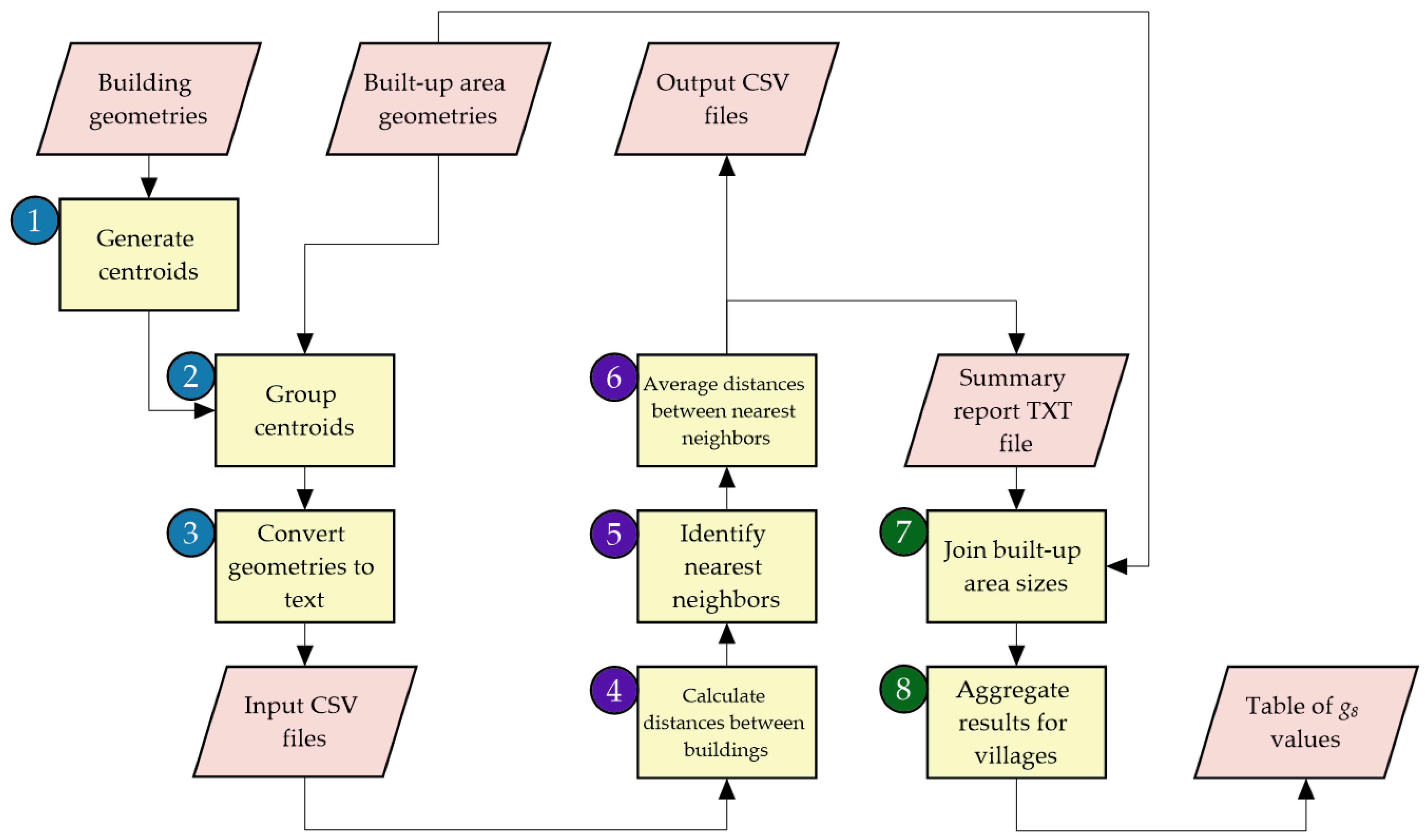
To automate the process of assigning nearest neighbours and calculating the indicator value $g_8$, dedicated software consisting of three components was developed: fully original scripts PAW g8 g9 KOMIWOJAŻER p1 1.4.py and PAW g8 ŚREDNIA ODL NAJBL SASIADA W OBSZ ZAB p2 2.1.py and a main program G8_06.cpp, developed with partial assistance from the artificial intelligence model ChatGPT 4o. The general workflow of the algorithm is presented in Figure 2.

Steps 1–3, which involved the conversion of vector spatial data into text files with a defined structure, were performed using the script PAW g8 g9 KOMIWOJAŻER p1 1.4.py. Steps 4–6, implementing the nearest neighbour assignment algorithm, are executed by the program G8_06.cpp. Steps 7–8, involving the final calculation of the indicator value $g_8$ and generation of output files, are performed by the script PAW g8 ŚREDNIA ODL NAJBL SASIADA W OBSZ ZAB p2 2.1.py. The result of the complete procedure is a set of indicator values for the analysed area or group of areas.

3.4.9. Length of the Approximate Hamiltonian Cycle for All Buildings in a Village ($g_9$)

The issue of the complexity and time consumption of surveying team mobility during fieldwork, beyond the previously discussed matters of building compactness and density within individual clusters, also encompasses the problem of building distribution relative to the overall land consolidation area. This spatial characteristic is addressed by the length of the Hamiltonian cycle for all buildings in a village, which serves as a practical implementation of the travelling salesman problem to quantify the total effort required for surveyors to move between all settlement points [59].

The indicator $g_9$ represents the length of an approximate Hamiltonian cycle covering the centroids of all buildings within the analysed village. Owing to the computational complexity of the problem (a practical realisation of the so-called travelling salesman problem [64]), the proposed solution is based on the greedy Nearest Neighbour (NN) algorithm [65].

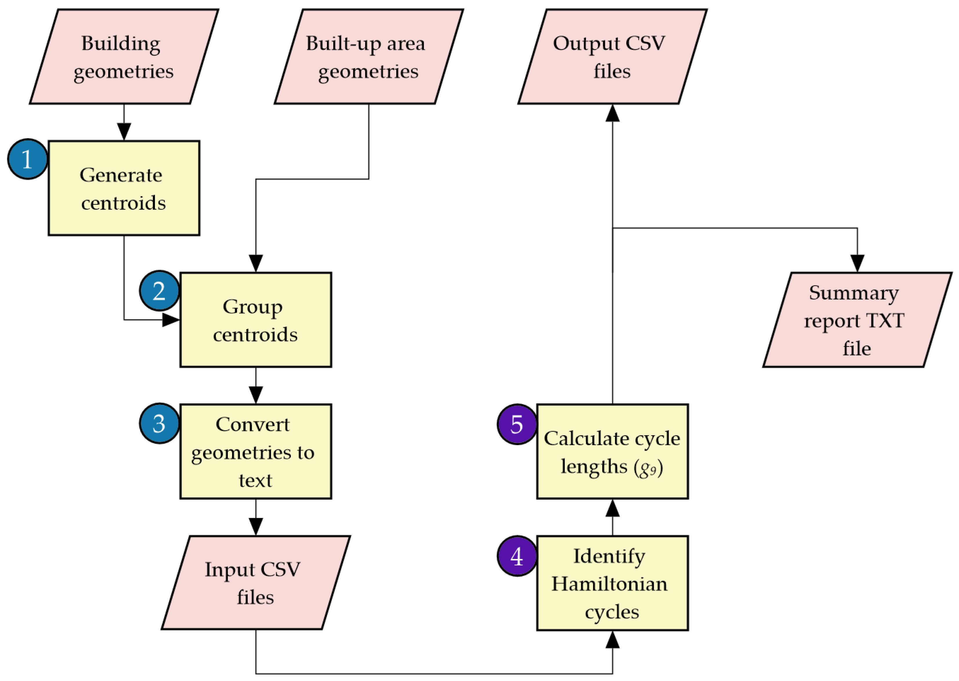
The nearest-neighbour algorithm was implemented in the dedicated program Komiwoj_NN_07.cpp, written in C++ with partial support from the artificial intelligence model ChatGPT 4o. The workflow of the computational procedure is illustrated in Figure 3.

The input data for the main algorithm were obtained by processing building geometries and built-up areas using the script PAW g8 g9 KOMIWOJAŻER p1 1.4.py (steps 1–3). The Komiwoj_NN_07.cpp program then approximates Hamiltonian cycles and calculates the indicator values $g_9$ for the analysed villages (steps 4–5). The algorithm finds the minimum ID value among all buildings in the dataset. This ensures that the starting point for the calculation of the heuristic tour length is deterministic and remains the same every time the program is executed for a given village.

3.5. Application of the Tools to a Sample of 40 Villages

The developed algorithms were applied to calculate the settlement structure indicators for the selected areas. This step aimed to validate the computational algorithms and their implementation, as well as to obtain the data necessary for subsequent stages of the research programme, including the assessment of the influence of rural built-up areas on land consolidation difficulty.

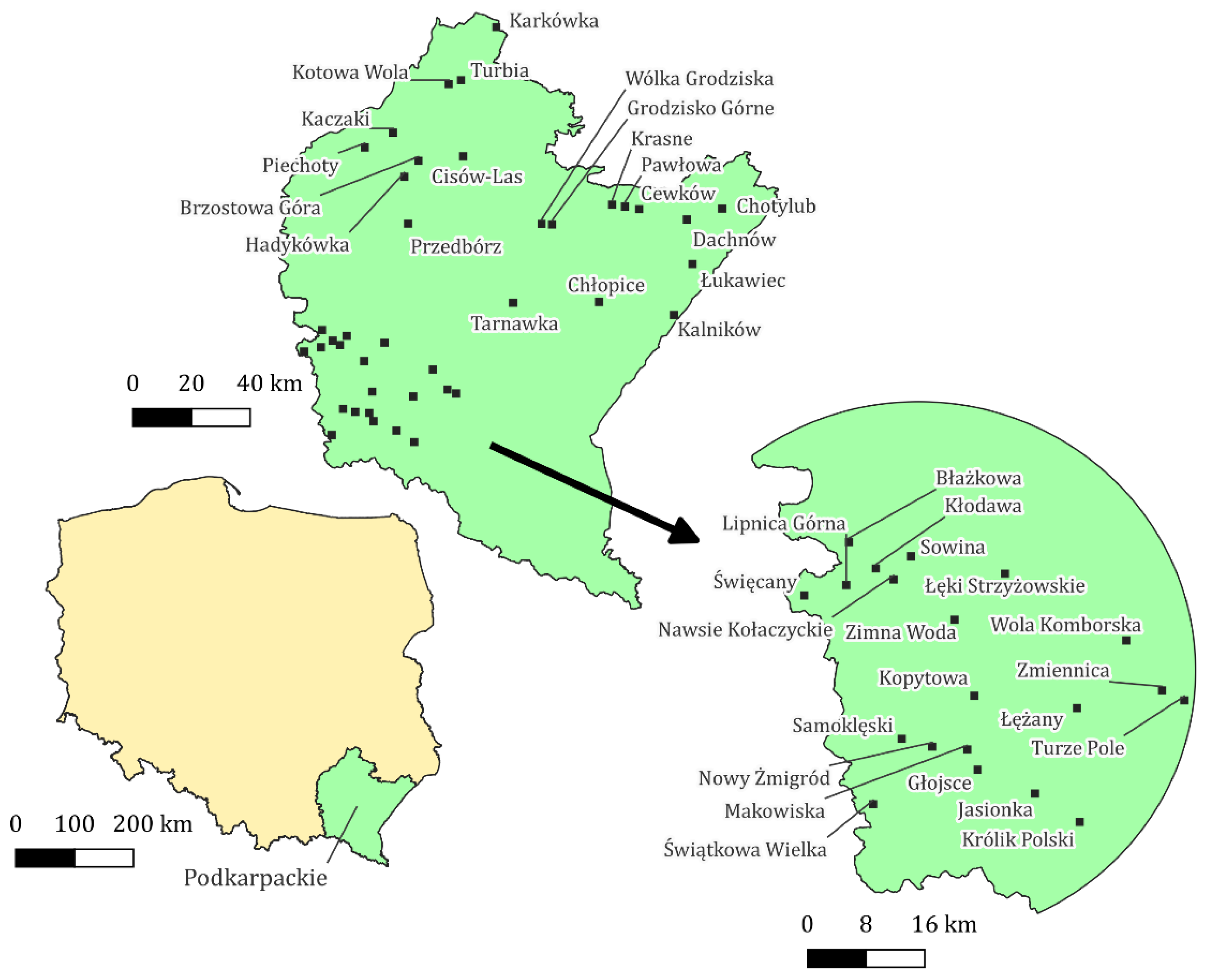
The study sample comprised 40 villages located in the Subcarpathian Voivodeship (southeastern Poland). The selection of the analysed areas considered the diversity of morphogenetic village types, which translates into the expected variability of indicator values. The locations of the analysed villages are presented in Figure 4.

The results were compiled in tabular form, together with the basic descriptive statistics of the indicators. Subsequently, the Shapiro–Wilk normality test [66] and Spearman’s $\rho$ rank correlation coefficients [67] and a Principal Component Analysis (PCA) [68,69] were performed. IBM SPSS Statistics 29 and Tibco Statistica 13.3 software were used for the computational process. The results are presented in Section 4.

4. Results

4.1. Built-Up Area Parameters for the Study Sample with Basic Statistics

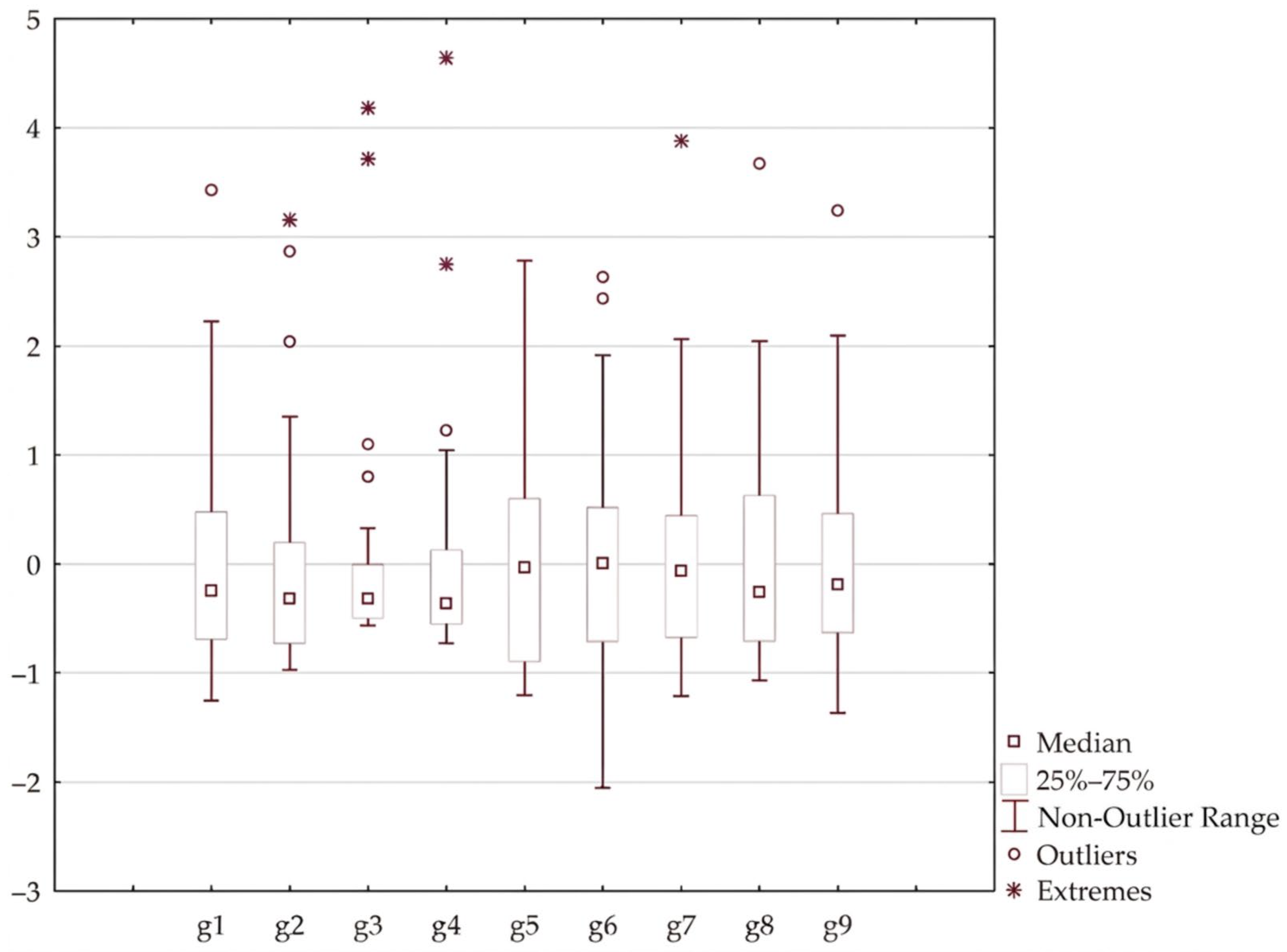
The values of the indicators $g_1$–$g_9$ and their basic descriptive statistics for the sample of 40 analysed villages are presented in

Table 2. Values of indicators $g_1$–$g_9$ for 40 villages in the Subcarpathian voivodeship including their basic descriptive statistics. Source: [59].

No	Village Name	${\mathit{g}}_1$ [m]	${\mathit{g}}_2$	${\mathit{g}}_3$ [ha]	${\mathit{g}}_4$	${\mathit{g}}_5$	${\mathit{g}}_6$ [1/ha]	${\mathit{g}}_7$ [1/ha]	${\mathit{g}}_8$ [m]	${\mathit{g}}_9$ [km]
1.	Błażkowa	1703.16	60.47	1.72	58	495	4.97	0.26	36.75	56.75
2.	Brzostowa Góra	1137.20	10.67	7.64	14	690	6.45	0.40	24.23	39.40
3.	Cewków	5723.72	38.53	20.12	7	983	6.98	0.23	21.08	47.10
4.	Chłopice	1524.90	30.73	9.60	7	384	5.71	0.62	24.28	25.72
5.	Chotylub	3102.35	33.50	8.93	4	309	8.65	0.12	21.03	22.53
6.	Cisów Las	1295.12	11.70	9.90	2	118	5.96	0.25	24.64	7.22
7.	Dachnów	2662.99	80.67	105.48	1	463	4.39	0.15	28.51	27.75
8.	Głojsce	2294.51	29.97	34.41	2	347	5.04	0.44	20.77	21.74
9.	Grodzisko Górne	4047.61	23.32	10.19	15	885	5.79	0.48	22.10	53.00
10.	Hadykówka	2364.30	18.53	11.49	5	403	7.01	0.80	22.39	21.14
11.	Jasionka	2263.29	13.24	41.62	2	402	4.83	0.49	22.49	17.90
12.	Kaczaki	1369.43	43.31	17.23	4	413	5.99	0.65	25.42	22.81
13.	Kalników	899.26	13.01	4.24	14	268	4.52	0.11	31.76	32.66
14.	Karkówka	1062.77	17.94	6.58	4	173	6.58	0.63	22.35	9.71
15.	Kłodawa	1230.66	10.78	4.29	6	113	4.39	0.52	33.25	9.05
16.	Kopytowa	1918.00	55.82	6.11	17	454	4.37	0.51	28.55	37.36
17.	Kotowa Wola	1573.08	25.41	6.82	14	509	5.33	0.44	23.88	33.88
18.	Krasne	728.90	18.10	1.71	13	178	8.00	0.22	26.81	14.94
19.	Królik Polski	2476.57	17.51	22.96	2	255	5.55	0.24	23.73	15.53
20.	Lipnica Górna	502.64	17.35	1.27	21	167	6.25	0.32	26.56	18.40
21.	Łęki Strzyżowskie	4361.18	64.04	5.97	15	434	4.84	0.40	28.72	36.16
22.	Łężany	2250.98	22.35	116.81	1	501	4.29	1.57	41.01	26.27
23.	Łukawiec	1713.82	33.25	4.55	15	385	5.65	0.11	28.44	31.83
24.	Makowiska	1186.08	13.76	5.50	5	123	4.47	0.22	28.05	11.69
25.	Nawsie Kołaczyckie	1620.71	28.44	5.63	15	335	3.96	0.58	33.41	27.32
26.	Nowy Żmigród	3187.26	53.48	14.01	6	530	6.30	0.64	23.69	29.51
27.	Pawłowa	439.69	10.16	1.45	10	129	8.89	0.08	27.20	17.78
28.	Piechoty	1083.12	8.07	8.90	2	120	6.74	0.39	23.14	7.55
29.	Przedbórz	2941.94	55.09	3.49	30	587	5.61	0.40	26.01	47.23
30.	Samoklęski	1574.67	33.16	7.43	6	163	3.65	0.16	32.96	16.93
31.	Sowina	955.47	33.76	1.36	33	280	6.23	0.34	35.47	32.07
32.	Świątkowa Wielka	638.03	9.04	2.24	8	96	5.35	0.06	36.42	10.14
33.	Święcany	606.87	19.37	1.17	89	584	5.63	0.29	43.41	73.34
34.	Tarnawka	2641.40	100.60	2.15	14	156	5.17	0.09	36.17	20.68
35.	Turbia	2425.73	28.13	19.33	7	814	6.02	0.91	20.88	33.71
36.	Turze Pole	2334.05	24.16	15.61	5	503	6.44	1.03	22.36	24.88
37.	Wola Komborska	642.84	16.18	1.74	22	221	5.76	0.43	29.82	22.85
38.	Wólka Grodziska	1380.10	13.32	10.53	6	368	5.82	0.59	23.91	23.89
39.	Zimna Woda	1017.87	14.07	34.28	1	106	3.09	0.42	34.97	6.75
40.	Zmiennica	1264.43	107.64	1.88	15	132	4.68	0.17	55.29	23.64
	Mean	1853.67	31.47	14.91	12.93	364.40	5.63	0.42	28.55	26.47
	Median	1573.88	23.74	7.13	7.00	357.50	5.64	0.40	26.69	23.77
	Std. Dev.	1114.19	23.81	24.06	16.19	219.62	1.22	0.29	7.19	14.28
	Minimum	439.69	8.07	1.17	1.00	96.00	3.09	0.06	20.77	6.75
	Maximum	5723.72	107.64	116.81	89.00	983.00	8.89	1.57	55.29	73.34
	Q1	1078.03	13.99	3.18	4.00	166.00	4.79	0.22	23.55	17.57
	Q3	2379.66	34.95	14.41	15.00	496.50	6.26	0.54	33.03	32.92
	CV (%)	60.1%	75.7%	161.4%	125.3%	60.3%	21.7%	69.8%	25.2%	54.0%

, while their distribution, after standardisation, is illustrated in Figure 5.

The values obtained for the individual indicators exhibited considerable variation in both range and distribution. This phenomenon results from the application of different computational formulas and measurement units and the deliberate selection of villages with diverse spatial characteristics for parameterisation purposes. Relatively high values of the coefficient of variation (CV) were observed for the variables corresponding to the surface area of built-up areas $g_3$ and $g_4$ the number of built-up areas. In contrast, relatively low variability was observed for the variables describing $g_6$ the average number of buildings per 1 ha of built-up areas and $g_8$ the average distance between buildings within a built-up area.

4.2. Assessment of the Distributions of Calculated Indicator Values

The results of the normality test for the variables $g_1$–$g_9$ performed using the Shapiro–Wilk method are presented in

Table 3. Results of the Shapiro–Wilk normality test for the variables $g_1$–$g_9$. Source: [59].

Variable	Statistic ($\mathit{W}$)	$\mathit{d}\mathit{f}$ (Degrees of Freedom)	$\mathit{p}$ (Significance)
$g_1$	0.891	40	0.001
$g_2$	0.807	40	<0.001
$g_3$	0.538	40	<0.001
$g_4$	0.631	40	<0.001
$g_5$	0.913	40	0.005
$g_6$	0.966	40	0.276
$g_7$	0.865	40	<0.001
$g_8$	0.856	40	<0.001
$g_9$	0.924	40	0.010

.

Among the analysed variables, only the indicator $g_6$ exhibited characteristics consistent with a normal distribution. For the remaining indicators, the normality hypothesis was rejected. Particularly low test statistics were observed for the indicators corresponding to $g_3$ the surface area of built-up areas and $g_4$ the number of built-up areas. The observed values of the test statistics imply asymmetry in the distributions of most variables.

4.3. Spearman’s Rank Correlation Coefficients (ρ) Between Indicators

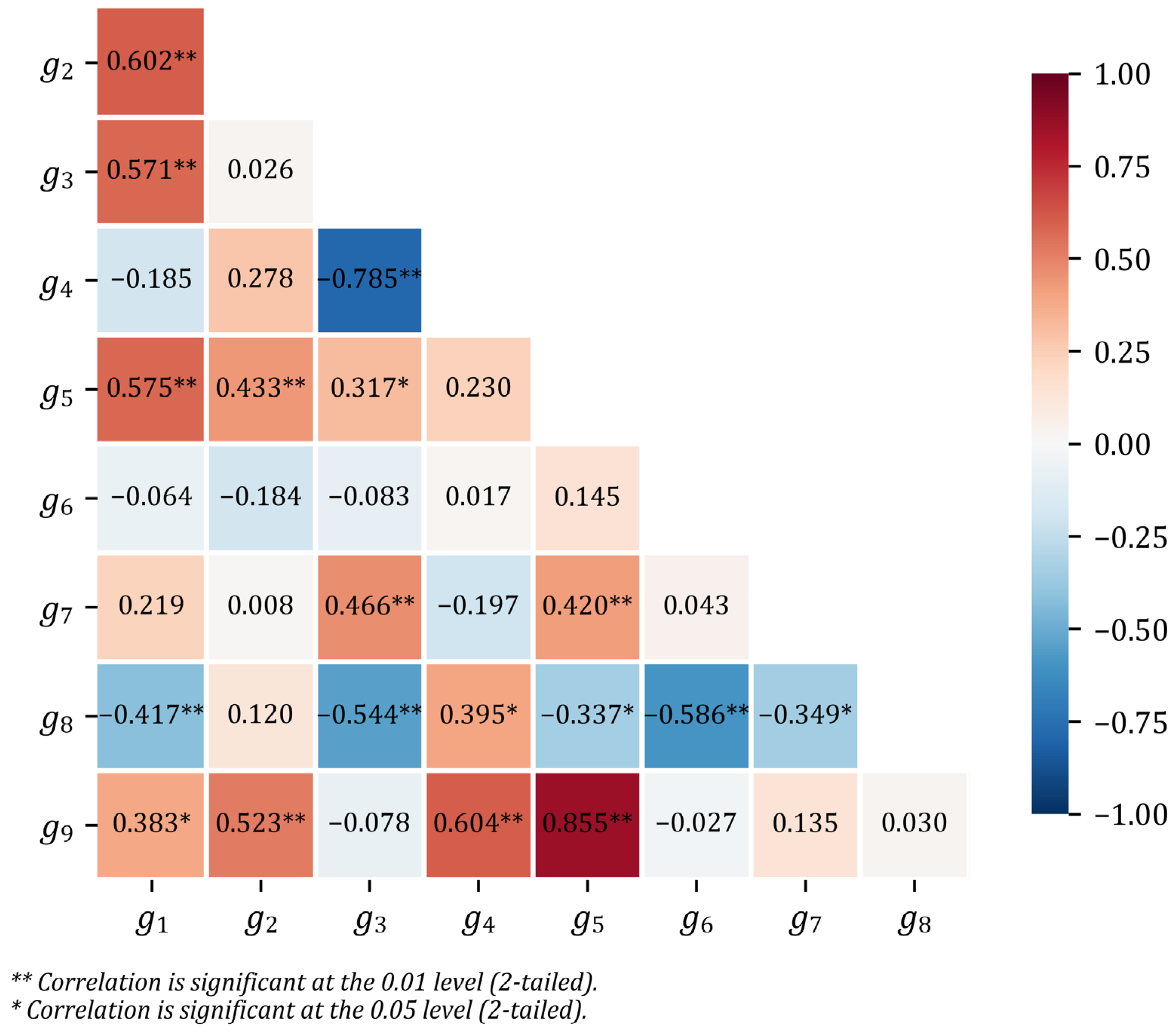
The Spearman’s rank correlation coefficients (ρ) for the variables $g_1$–$g_9$ are presented as a heatmap in Figure 6.

Statistically significant strong correlations were observed for pairs of variables corresponding to $g_5$ and $g_9$ (positive correlation), and to $g_3$ and $g_4$ (negative correlation). In addition, numerous pairs of variables exhibit moderate or weak correlations.

4.4. Principal Component Analysis (PCA)

To address the potential redundancy and multicollinearity identified in the Spearman correlation analysis (Section 4.3), a Principal Component Analysis (PCA) was performed on the indicators $(g_1$–$g_9).$ The results are presented in

Table 4. Principal Component Analysis (PCA) for the variables $g_1$–$g_9$. Source: own elaboration.

Component	${\mathit{R}}^2\mathit{X}$	${\mathit{R}}^2\mathit{X}$ (Cumulative)	Eigenvalues
PC1	28.14%	28.14%	2.5325
PC2	24.55%	52.69%	2.2095
PC3	19.35%	72.04%	1.7419

.

The PCA results indicate that the first three principal components (PCs) have eigenvalues greater than 1 and collectively explain 72.04% of the total variance in the dataset. This exceeds the widely accepted threshold of 70% in exploratory research [70], confirming that the reduction in dimensionality does not result in a significant loss of information. A factor loading matrix for these components is presented in

Table 5. Factor loading matrix for principal components PC1–PC3. Source: own elaboration.

Indicator	PC1	PC2	PC3
$g_1$	0.7269	0.3819	−0.0632
$g_2$	0.3867	−0.3854	−0.3850
$g_3$	0.2140	0.4032	−0.7090
$g_4$	0.3701	−0.7785	0.2713
$g_5$	0.9251	0.2297	0.1363
$g_6$	−0.0054	0.2835	0.7637
$g_7$	0.2633	0.4982	−0.3588
$g_8$	−0.0903	−0.7805	−0.4918
$g_9$	0.8593	−0.3949	0.2027

.

As shown in Table 5, component PC1 is strongly defined by the physical scale and intensity of development. It shows high positive loadings for the number of buildings ($g_5$), the length of the approximate Hamiltonian cycle for all buildings in a village ($g_9$), and the length of built-up areas ($g_1$). This component effectively aggregates variables describing the overall “size” of the village settlement. PC2 represents the spatial configuration and fragmentation of the settlement. It is characterised by high negative loadings for the average distance between buildings within a built-up area ($g_8$) and the number of built-up areas ($g_4$). PC3 captures the internal density and cluster characteristics. It shows a strong positive loading for the average number of buildings per 1 ha of built-up areas ($g_6$), and a high negative loading for the surface area of built-up areas ($g_3$). This component distinguishes between small, densely packed clusters and large, low-density built-up zones.

5. Discussion

The achievement of the research objectives provides a methodological foundation for rural development research related to land consolidation. By introducing a formalised and automated approach to settlement characterisation, this study establishes a framework for the further prediction of land consolidation difficulty. While the current results are based on a sample of 40 villages, which limits the immediate generalisability of the findings, the high cumulative variance explained by the PCA (72.04%) confirms the robustness of the selected indicators in capturing settlement diversity. The publication of the developed tools in a public repository enables full reproducibility of the study, including further validation of the methodology, extension and refinement of the algorithms, and calculation of indicator values for other regions. The development of a fully validated predictive model remains a subject for the subsequent, empirical stage of this research programme.

This study corroborates and extends the widely accepted view on the necessity of implementing automated computational models in the planning and implementation of land consolidation works, as highlighted by Demetriou [71]. The consideration of rural settlement characteristics in agricultural land management policy, in line with the argument of Barbosa et al. [72], supports the pursuit of sustainable rural development based on coherent agricultural and spatial policies.

The proposed approach to settlement characterisation also introduces a potential new tool for rural research. The methodological assumptions are consistent with multiparameter approaches to rural settlement assessment, implemented by researchers using both cadastral-topographic geometric data [73] and photogrammetric and remote sensing imagery [74].

However, the practical implementation of the results of this study requires an understanding and consideration of the specificity of the developed indicators, including limitations arising from the adopted methodology for their selection and calculation. The statistical analysis of the output data provided important insights into the expected distributions of settlement indicators and their applicability in predicting land consolidation difficulty. Low values of the Shapiro–Wilk test statistic, typically coexisting with high coefficients of variation (CV), may indicate a risk of model distortion when using traditional parametric methods, due to the presence of villages with atypical or non-standard settlement patterns. The results obtained for the indicators corresponding to $g_3$ the surface area of built-up areas and the $g_4$ number of built-up areas indicate significant disparities in the spatial distribution of settlements, which, according to Kuczyńska and Głowacki [75], is a natural phenomenon in the Carpathian region, including south-eastern Poland. Consequently, the observed non-normality implies that subsequent predictive modelling will necessitate the use of non-parametric approaches or robust regression techniques, which are less sensitive to distributional assumptions and outliers. Alternatively, data transformation methods may be implemented to approximate normality before applying parametric models.

The presence of strongly correlated variable pairs, such as $g_5$ the number of buildings and $g_9$ the length of the approximate Hamiltonian cycle for all buildings in a village, as well as the $g_3$ surface area of built-up areas and $g_4$ the number of built-up areas, may additionally indicate the need to eliminate certain variables from the land consolidation difficulty model or to aggregate or assign weights to selected indicators. These observations should be considered when developing a mathematical model. It is also recommended that the analysis be repeated on other village datasets and that the results be compared.

Regarding the analysis of correlations between the built-up area indicators, it should be noted that the Spearman correlation coefficients do not provide a sufficient basis for direct application in predictive modelling. A comprehensive statistical analysis and the construction of a predictive model will be presented in a subsequent stage of the research programme. At this point, the aforementioned coefficients should be regarded as a descriptive mathematical summary of the current dataset, providing valuable insights for further research.

However, the high cumulative explained variance ($R^{2}X$) confirms that the proposed set of indicators ($g_1$–$g_9$) provides a comprehensive mathematical description of the rural settlement structures. By transforming the original, partially redundant variables into three independent dimensions, the PCA successfully addresses the issue of multicollinearity. This approach provides a stable and objective foundation for the subsequent development of predictive models to estimate land consolidation difficulty, ensuring that the final assessment is not distorted by overlapping information.

A significant limitation in optimising the selection of settlement indicators for assessing land consolidation difficulty was the almost complete absence of analogous or related studies in the scientific and technical literature, which also complicates the discussion of the obtained results. According to the authors, in light of these limitations, particular attention should be paid to the validation of the developed tools and the evaluation of the results using available statistical methods. Expert opinions, particularly from practitioners experienced in planning and implementing land consolidation procedures, may also constitute an important source of technical knowledge.

6. Conclusions

The research conducted successfully addressed the identified research gap within the defined study aims. A particularly significant contribution of this study is the proposal of an unambiguous set of numerical characteristics for rural built-up patterns, including a complete calculation methodology and original software that enables the automation of computational processes.

The experimental implementation on a sample of 40 villages in the Subcarpathian Voivodeship confirmed that the proposed indicators effectively capture the high natural variability of settlement patterns in this region. Furthermore, the application of Principal Component Analysis (PCA) demonstrated that 72.04% of the dataset’s variance is explained by three independent components, effectively resolving the issue of multicollinearity among the indicators.

The parameterisation and interpretation presented mark the completion of the first stage of a comprehensive research programme. Future work will focus primarily on the development of a predictive model to estimate the technical difficulty of land consolidation based on these spatial characteristics. The current built-up pattern indicators ($g_1$–$g_9$) will also be evaluated using various samples of rural areas located in different regions and characterised by different levels of variability. Subsequently, the proposed methodology will be optimised for use in diverse regions.

In the long term, additional potential determinants of land consolidation difficulty will be identified and parameterized. The overarching goal of the entire research programme is to develop a comprehensive methodology for estimating land consolidation difficulty. This will facilitate a revision of current strategic and technical assumptions, increasing the economical and practical efficiency of consolidation works.

References

- Leń, P.; Maciąg, K.; Maciąg, M.; Wójcik-Leń, J.; Kocur-Bera, K. Proposed Algorithm for the Optimisation of the Process of Generating the Geometry of Land Use/Soil Valuation Classes for Land Consolidation. Sustainability 2023, 15, 8430. [Google Scholar] [CrossRef]
- Leń, P.; Maciąg, K.; Maciąg, M.; Wójcik-Leń, J.; Kocur-Bera, K. Automated Processing of Data in the Comparative Estimation of Land Value During Land Consolidation Works. Sustainability 2023, 15, 8110. [Google Scholar] [CrossRef]
- Leń, P.; Maciąg, M.; Maciąg, K. Design of an Automated Algorithm for Delimiting Land Use/Soil Valuation Classes as a Tool Supporting Data Processing in the Land Consolidation Procedure. Sustainability 2023, 15, 8486. [Google Scholar] [CrossRef]
- Janus, J.; Ertunç, E. Differences in the effectiveness of land consolidation projects in various countries and their causes: Examples of Poland and Turkey. Land Use Policy 2021, 108, 105542. [Google Scholar] [CrossRef]
- Cay, T.; Uyan, M. Evaluation of reallocation criteria in land consolidation studies using the Analytic Hierarchy Process (AHP). Land Use Policy 2013, 30, 541–548. [Google Scholar] [CrossRef]
- Aslan, S.T.A.; Kirmikil, M.; Gündoğdu, K.S.; Arici, I. Reallocation model for land consolidation based on landowners’ requests. Land Use Policy 2018, 70, 463–470. [Google Scholar] [CrossRef]
- Colombo, S.; Perujo-Villanueva, M. A practical method for the ex-ante evaluation of land consolidation initiatives: Fully connected parcels with the same value. Land Use Policy 2019, 81, 463–471. [Google Scholar] [CrossRef]
- Pašakarnis, G.; Maliene, V. Towards sustainable rural development in Central and Eastern Europe: Applying land consolidation. Land Use Policy 2010, 27, 545–549. [Google Scholar] [CrossRef]
- Dudzińska, M.; Bacior, S.; Prus, B. Considering the level of socio-economic development of rural areas in the context of infrastructural and traditional consolidations in Poland. Land Use Policy 2018, 79, 759–773. [Google Scholar] [CrossRef]
- Leń, P.; Maciąg, M.; Siejka, M.; Maciąg, K.; Kocur-Bera, K.; Rapiński, J. A New Method for Assessing Land Consolidation Urgency, including Market Value. Sustainability 2024, 16, 835. [Google Scholar] [CrossRef]
- Maciąg, M.; Maciąg, K.; Kiszka, K.; Leń, P. Rzecz o dobrej kulturze rolnej. Przegląd Geod. 2024, 9, 19–22. [Google Scholar] [CrossRef]
- Maciąg, M.; Maciąg, K.; Leń, P. Algorithm for Evaluating the Difficulty of Land Consolidation Using Cadastral Data. Sustainability 2024, 16, 5648. [Google Scholar] [CrossRef]
- van Dijk, T. Scenarios of Central European land fragmentation. Land Use Policy 2003, 20, 149–158. [Google Scholar] [CrossRef]
- Jürgenson, E. Land reform, land fragmentation and perspectives for future land consolidation in Estonia. Land Use Policy 2016, 57, 34–43. [Google Scholar] [CrossRef]
- Sklenicka, P. Applying evaluation criteria for the land consolidation effect to three contrasting study areas in the Czech Republic. Land Use Policy 2006, 23, 502–510. [Google Scholar] [CrossRef]
- Mihara, M. Effects of Agricultural Land Consolidation on Erosion Processes in Semi-Mountainous Paddy Fields of Japan. J. Agric. Eng. Res. 1996, 64, 237–247. [Google Scholar] [CrossRef]
- Luo, W.; Timothy, D.J. An assessment of farmers’ satisfaction with land consolidation performance in China. Land Use Policy 2017, 61, 501–510. [Google Scholar] [CrossRef]
- Abubakari, Z.; van der Molen, P.; Bennett, R.M.; Kuusaana, E.D. Land consolidation, customary lands, and Ghana’s Northern Savannah Ecological Zone: An evaluation of the possibilities and pitfalls. Land Use Policy 2016, 54, 386–398. [Google Scholar] [CrossRef]
- Ertunç, E.; Çay, T.; Haklı, H. Modeling of reallocation in land consolidation with a hybrid method. Land Use Policy 2018, 76, 754–761. [Google Scholar] [CrossRef]
- Krzemieniecki, K.; Mika, M. Analysis of demand for land consolidation works in Poland—A case study of the Bałtów commune. Land Use Policy 2025, 150, 107451. [Google Scholar] [CrossRef]
- Mika, M.; Leń, P.; Oleniacz, G.; Kurowska, K. Study of the effects of applying a new algorithm for the comprehensive programming of the hierarchization of land consolidation and exchange works in Poland. Land Use Policy 2019, 88, 104182. [Google Scholar] [CrossRef]
- Janus, J.; Taszakowski, J. Spatial differentiation of indicators presenting selected barriers in the productivity of agricultural areas: A regional approach to setting land consolidation priorities. Ecol. Indic. 2018, 93, 718–729. [Google Scholar] [CrossRef]
- Leń, P. An algorithm for selecting groups of factors for prioritization of land consolidation in rural areas. Comput. Electron. Agric. 2018, 144, 216–221. [Google Scholar] [CrossRef]
- Janus, J.; Markuszewska, I. Forty years later: Assessment of the long-lasting effectiveness of land consolidation projects. Land Use Policy 2019, 83, 22–31. [Google Scholar] [CrossRef]
- Malashevskyi, M.; Malashevska, O. Land Consolidation Considering Natural Afforestation. Geomat. Environ. Eng. 2022, 16, 5–19. [Google Scholar] [CrossRef]
- Montefiori, L.; Bassi, I.; Dosso, R.; Ferrario, V.; Iseppi, L. The Role of Land Consolidation Associations in Enhancing Mountain Attractiveness: The Case of ASFO Erbezzo. Sustainability 2025, 17, 8275. [Google Scholar] [CrossRef]
- Wan, R.; Yu, H.; Zhang, D.; Yang, B.; Huang, Y. Effects of Comprehensive Land Consolidation on Farmers’ Livelihood Under Different Terrain Gradients. Land 2025, 14, 871. [Google Scholar] [CrossRef]
- Hiironen, J.; Riekkinen, K. Agricultural impacts and profitability of land consolidations. Land Use Policy 2016, 55, 309–317. [Google Scholar] [CrossRef]
- Liu, Q.; Fu, Y.; Teng, G.; Ma, J.; Yao, Y.; Chen, L. Spatio-Temporal Evolution Characteristics of Land Consolidation in the Coastal Regions: A Typical Case Study of Lianyungang, China. Land 2025, 14, 1776. [Google Scholar] [CrossRef]
- Shi, C. Is a Self-Organized Structure Always the Best Choice for Collective Members? A Counterexample in China’s Urban–Rural Construction Land Linkage Policy. Land 2025, 14, 1807. [Google Scholar] [CrossRef]
- Czarnecka, A.; Stępnik, K.; Krupowicz, W.; Home, R. Integrating place attachment and social capital in land consolidation procedures for sustainable landscape development. J. Rural Stud. 2026, 123, 104095. [Google Scholar] [CrossRef]
- Pun, R.; Joshi, N.P.; Pun, S. Factors influencing farmers’ preference for farmland consolidation in Nepal: Evidence from randomized conjoint experiment. Agric. Syst. 2024, 219, 104038. [Google Scholar] [CrossRef]
- Bonadonna, A.; Rostagno, A.; Beltramo, R. Improving the Landscape and Tourism in Marginal Areas: The Case of Land Consolidation Associations in the North-West of Italy. Land 2020, 9, 175. [Google Scholar] [CrossRef]
- Zhang, X.; Ye, Y. Advances in Land Consolidation and Land Ecology. Land 2024, 13, 1897. [Google Scholar] [CrossRef]
- Lu, H.; Shi, H.; Li, B.; Xu, D. The Impact of Whole Region Comprehensive Land Consolidation on Ecological Vulnerability: Evidence from Township Panel Data in Zhejiang Province. Land 2025, 14, 2291. [Google Scholar] [CrossRef]
- Zhang, Q.; Zhang, T. Land Consolidation Design Based on an Evaluation of Ecological Sensitivity. Sustainability 2018, 10, 3736. [Google Scholar] [CrossRef]
- Janus, J.; Łopacka, M.; John, E. Land consolidation in mountain areas. Case study from southern Poland. Geod. Cartogr. 2017, 66, 241–251. [Google Scholar] [CrossRef][Green Version]
- Zaborski, B. O Kształtach wsi w Polsce i Ich Rozmieszczeniu; Prace Komisji Etnograficznej Polskiej Akademii Umiejętności: Kraków, Poland, 1926. [Google Scholar]
- Meitzen, A. Siedelung und Agrarwesen der Westgermanen und Ostgermanen, der Kelten, Römer, Finnen und Slawen; W. Hertz: Berlin, Germany, 1895. [Google Scholar]
- Górak, J. Problemy ochrony zabytków rurystycznych na przykładzie wsi Pańków w woj. lubelskim. Ochr. Zabyt. 1971, 24, 203–206. [Google Scholar]
- Wich, U. Wiejska struktura przestrzenna i perspektywiczne kierunki jej zmian. Ann. Univ. Mariae Curie-Sklodowska Sect. H Oecon. 1975, 9, 99–111. [Google Scholar]
- Wójcik, M. Geografia wsi w Polsce. Studium Zmiany Podstaw Teoretyczno-Metodologicznych; Wydawnictwo Uniwersytetu Łódzkiego: Łódź, Poland, 2012. [Google Scholar] [CrossRef]
- Myga-Piątek, U. Krajobrazy Kulturowe. Aspekty Ewolucyjne i Typologiczne; Uniwersytet Śląski: Katowice, Poland, 2012. [Google Scholar]
- Szymańska, D. Geografia Osadnictwa; Wydawnictwo Naukowe PWN: Warszawa, Poland, 2013. [Google Scholar]
- Gibas, P.; Heffner, K. Koncentracja zabudowy na obszarach wiejskich. Wieś Rol. 2018, 2, 189–207. [Google Scholar] [CrossRef] [PubMed]
- Sudra, P. Zastosowanie wskaźników koncentracji przestrzennej w badaniu procesów urban sprawl. Przegląd Geogr. 2016, 88, 247–272. [Google Scholar] [CrossRef]
- Serafin, P. Zmiany w użytkowaniu gruntów oraz gęstość zabudowy na styku miasto—Obszar wiejski jako przejawy suburbanizacji Nowego Sącza. Pr. Nauk. Uniw. Ekon. Wrocławiu 2017, 467, 102–112. [Google Scholar] [CrossRef]
- Śleszyński, J. Propozycja kompleksowej koncepcji wskaźników zagospodarowania i ładu przestrzennego. Biul. Kom. Przestrz. Zagospod. Kraj. PAN 2013, 252, 176–231. [Google Scholar]
- Salata, T. Koncepcja znormalizowanej metody wyznaczania obszarów zabudowy. Zesz. Nauk. Uniw. Rol. Im. Hugona Kołłątaja Krak. 2019, 549, 426. [Google Scholar]
- Ustawa z Dnia 26 Marca 1982 r. o Scalaniu i Wymianie Gruntów. Dz. U. 2023 r. poz. 1197; 1982. Available online: https://isap.sejm.gov.pl/isap.nsf/DocDetails.xsp?id=WDU19820110080 (accessed on 30 August 2025).
- Instrukcja nr 1 Ministra Rolnictwa i Gospodarki Żywnościowej o Scalaniu i Wymianie Gruntów z Dnia 24 Marca 1983 r. GZ-g-630-1/83, 1983. Available online: https://www.studocu.com/pl/document/wojskowa-akademia-techniczna/geodezja-miejska/instrukcja-nr-1-ministra-o-scaleniu/118047433?sid=c5f88586-8520-4bde-acf6-9d5f6c8a35731783420737 (accessed on 30 August 2025).
- Podkarpackie Biuro Geodezji i Terenów Rolnych w Rzeszowie (PBGiTR). Zakładowy Katalog Norm Pracy. Opracowanie Projektu Scalenia Gruntów. Załącznik nr 3 do Zarządzenia nr 7/2009 z dnia 23 Czerwca 2009 r. Dyrektora PBGiTR w Rzeszowie; PBGiTR: Rzeszów, Poland, 2009.
- Dudzińska, M. Koncepcja Metodologii Doboru Determinant Wpływających na Wybór Miejsca Realizacji Scaleń Gruntów Rolnych; Wydawnictwo Uniwersytetu Warmińsko-Mazurskiego: Olsztyn, Poland, 2019. [Google Scholar]
- Przegon, W. Ochrona środowiska w projektach scaleniowych gruntów. Czas. Tech. Archit. 2007, 104, 269–275. [Google Scholar]
- Markuszewska, I. Plany urządzeniowo-rolne gmin jako narzędzie planowania prac scaleniowych. Probl. Ekol. Kraj. 2012, 33, 235–241. [Google Scholar]
- Jaroszewicz, J.; Radziszewska, W. Możliwości wykorzystania systemów informacji geograficznej w pracach scaleniowych. Infrastrukt. Ekol. Teren. Wiej. 2013, 1, 143–159. [Google Scholar]
- Zygmunt, M.; Ślusarski, M.; Gniadek, J.; Szewczyk, R. Issues of analytical design of land division with high value per hectare. Geomat. Landmanag. Landsc. 2018, 3, 55–61. [Google Scholar] [CrossRef]
- Decyzja Wojewody Podkarpackiego z Dnia 8 Kwietnia 2022 r. nr GK-II.7213.60.2021 w Przedmiocie Zatwierdzenia Projektu Scalenia Gruntów, 2022. Available online: https://www.inforlex.pl/dok/tresc,WSA.2023.005.013039610,Wyrok-WSA-w-Rzeszowie-z-dnia-16-maja-2023-r-sygn-II-SA-Rz-630-22.html (accessed on 30 August 2025).
- Maciąg, M. An Assessment of the Difficulty of Land Consolidation Works with Respect to Development Characteristics. Ph.D. Thesis, Rzeszów University of Technology, Rzeszów, Poland, 2026. [Google Scholar]
- Microsoft Global Building Footprints. Available online: https://github.com/microsoft/GlobalMLBuildingFootprints (accessed on 31 March 2026).
- OpenStreetMap. Available online: https://planet.openstreetmap.org (accessed on 31 March 2026).
- GitHub. Available online: https://github.com/maciag-mm/lcdifficulty_buildings (accessed on 31 March 2026).
- Litwin, U.; Szewczyk, R. Morfologia działek przyczynkiem kształtowania krajobrazu. Infrastrukt. Ekol. Teren. Wiej. 2012, 2, 39–48. [Google Scholar]
- Flood, M.M. The Travelling-Salesman Problem. Oper. Res. 1956, 4, 61–75. [Google Scholar] [CrossRef]
- Hurkens, C.A.J.; Woeginger, G.J. On the nearest neighbor rule for the traveling salesman problem. Oper. Res. Lett. 2004, 32, 1–4. [Google Scholar] [CrossRef]
- Shapiro, S.S.; Wilk, M.B. An Analysis of Variance Test for Normality (Complete Samples). Biometrika 1965, 52, 591–611. [Google Scholar] [CrossRef]
- Spearman, C. The Proof and Measurement of Association Between Two Things. Am. J. Psychol. 1904, 15, 72–101. [Google Scholar] [CrossRef] [PubMed]
- Pearson, K. On lines and planes of closest fit to systems of points in space. Lond. Edinb. Dublin Philos. Mag. J. Sci. 1901, 2, 559–572. [Google Scholar] [CrossRef]
- Hotelling, H. Analysis of a complex of statistical variables into principal components. J. Educ. Psychol. 1933, 24, 417–441. [Google Scholar] [CrossRef]
- Weeraratne, N.; Hunt, L.; Kurz, J. Optimizing PCA for Health and Care Research: A Reliable Approach to Component Selection. arXiv 2025, arXiv:2503.24248. [Google Scholar]
- Demetriou, D. The Development of an Integrated Planning and Decision Support System (IPDSS) for Land Consolidation; Springer: Cham, Switzerland, 2014. [Google Scholar] [CrossRef]
- Barbosa, V.; Santé-Riveira, I.; Crecente-Maseda, R.; Redondo, C.D.; Trinidad, J.P.; López, J.P.; Biempica, R.D.; Ferreira Neto, J.A. A New Spatial Criteria Method to Delimit Rural Settlements towards Boundaries Equity: Land Use Optimization for Decision Making in Galicia, NW Spain. Land 2022, 11, 800. [Google Scholar] [CrossRef]
- Yang, R.; Xu, Q.; Long, H. Spatial distribution characteristics and optimized reconstruction analysis of China’s rural settlements during the process of rapid urbanization. J. Rural Stud. 2016, 47, 413–424. [Google Scholar] [CrossRef]
- Zheng, X.; Wu, B.; Weston, M.V.; Zhang, J.; Gan, M.; Zhu, J.; Deng, J.; Wang, K.; Teng, L. Rural Settlement Subdivision by Using Landscape Metrics as Spatial Contextual Information. Remote Sens. 2017, 9, 486. [Google Scholar] [CrossRef]
- Kuczyńska, K.; Głowacki, W. Typologia osadnictwa Karpackiego Regionu Rozwoju. Probl. Rozw. Miast 2009, 6, 62–75. [Google Scholar]