Impact of Landscape Composition and Configuration on Urban Heat Island Intensity in Zhengzhou Urban Area: Based on Nonlinear Response Patterns and Region-Specific Thresholds

Abstract

Rapid urbanization has significantly altered urban landscape composition and configuration, making it a key driver exacerbating the urban heat island (UHI) effect. As a rapidly expanding inland city in Central China, Zhengzhou is highly sensitive to changes in landscape composition and spatial configuration. Therefore, clarifying the nonlinear relationship between landscape patterns and the urban thermal environment is of great significance for sustainable urban planning and thermal environment regulation. Taking the main urban area of Zhengzhou as the study area, this paper retrieves land surface temperature (LST) using the radiative transfer equation method based on Landsat 8 remote sensing images from August 2015 to August 2024, and constructs the surface urban heat island intensity (SUHII) index. By integrating multi-dimensional landscape pattern indices, the XGBoost machine learning model, and the SHAP interpretability method, this study systematically analyzes the nonlinear response mechanisms of landscape composition and configuration to SUHII, key regulatory thresholds, and their changes between 2015 and 2024. The results show that: (1) The SUHII in Zhengzhou was substantially higher in 2024 than in 2015. The area proportions of strong and extremely strong heat islands were higher in 2024 (26.16% and 2.34%) than in 2015 (2.22% and 0.12%), and the thermal environment differed between 2015 and 2024, shifting from a localized patch pattern to a more continuously expanding pattern. (2) Landscape area-related indices are the key factors. The areas of green space and water bodies, along with the landscape diversity index, show significant negative correlations, while built-up area and aggregation index show significant positive correlations. (3) SHAP feature importance indicates that water body area is the primary cooling factor, whereas built-up area is the primary warming factor, jointly dominating the spatial pattern of the thermal environment in Zhengzhou. (4) Landscape composition and configuration exhibit significant nonlinear responses to SUHII with region-specific thresholds, and these thresholds were higher/lower in 2024 than in 2015, suggesting a possible association with urban expansion. Specifically, stable cooling effects occurred when the water body area exceeded 3.5 km² in 2015, with the threshold rising to 4.2 km² in 2024. The warming threshold for built-up area decreased from 18.8 km² to 8.5 km², suggesting a higher sensitivity of the thermal environment to built-up area expansion in 2024 compared to 2015, characterized by a regulation pattern of “dominant scale effect and weakened configuration effect”. This study identifies thresholds specific to Zhengzhou’s main urban area at two time points (2015 and 2024), providing quantitative support and scientific basis for blue–green space optimization, precise heat island mitigation, and territorial spatial planning in Zhengzhou. These findings are based on a comparison of two time points (2015 and 2024) and do not directly capture continuous temporal dynamics.

1. Introduction

The urban heat island (UHI) effect is one of the most typical urban ecological and environmental issues in the context of rapid urbanization. It has become an important factor constraining urban sustainable development, resident health, and the process of achieving the “dual carbon” goals and building livable cities [1,2]. Existing studies have shown that the formation of the UHI effect is not only closely related to land cover change, built-up area expansion, and population agglomeration, but is also jointly driven by multiple factors such as anthropogenic heat emissions, air pollution, and meteorological conditions. Among these, land use transformation and changes in landscape spatial configuration are considered the most direct and manageable factors affecting the urban thermal environment. As urban built-up areas expand rapidly, the area proportions, spatial aggregation levels, and compositional arrangements of different landscape types significantly influence UHI Intensity by altering surface albedo, evapotranspiration, and heat transfer processes [3,4,5].

Previous studies have consistently demonstrated two key findings regarding landscape composition and configuration and the urban thermal environment. First, landscape composition—particularly the area of built-up land, green space, and water bodies—is the dominant factor regulating SUHII, with blue–green spaces providing cooling effects and built-up land generating warming effects [6,7,8]. Second, landscape spatial configuration (e.g., patch aggregation, fragmentation, and diversity) plays a secondary but non-negligible modulating role. However, most existing research suffers from three critical limitations. First, the majority of studies are static, relying on single-year or short-term data, which cannot capture how the relationship between landscape patterns and SUHII evolves under rapid urbanization [9]. Second, they predominantly assume linear relationships, thereby overlooking potential nonlinear response patterns and, more importantly, the existence of region-specific thresholds—i.e., critical values beyond which a landscape factor’s warming or cooling effect intensifies or weakens significantly [10,11]. Third, even when thresholds are mentioned, their dynamic shift as urban expansion proceeds has rarely been investigated [12,13,14]. Consequently, planners lack quantitative, stage-specific guidelines for blue–green space optimization and built-up land control.

To address these gaps, this study makes three contributions:

(1) It provides a cross-stage comparison of SUHII and landscape thresholds between 2015 and 2024, showing that the cooling threshold for water bodies was higher in 2024 (4.2 km²) than in 2015 (3.5 km²), while the warming threshold for built-up land was lower (8.5 km² vs. 18.8 km²).

(2) It quantifies empirical uncertainty ranges for these thresholds based on SHAP dependence plots, offering a transparent, data-driven measure of threshold variability that is rarely reported in similar studies.

(3) It translates these thresholds into grid-specific planning recommendations (e.g., water bodies >4.2 km² per 500 m grid; built-up patches <8.5 km²) that can be directly used by urban planners in Zhengzhou. To address these gaps, this study provides empirical evidence on how landscape thresholds differ between two distinct urbanization stages (2015 and 2024) in a rapidly growing inland megacity. Rather than introducing novel algorithms, our contribution lies in: (1) quantifying the observed differences in cooling and warming thresholds for water bodies and built-up land over this decade; (2) reporting empirical uncertainty ranges derived from SHAP dependence plots to transparently characterize threshold variability; and (3) translating these stage-specific thresholds into grid-based, actionable planning benchmarks (e.g., water area > 4.2 km² per 500 m grid; built-up patch < 8.5 km²) that can directly inform blue–green space optimization and built-up land control in Zhengzhou. While the XGBoost-SHAP framework is standard, its application to compare thresholds across two time points and link them to spatial planning units constitutes the main novelty of this work.

As a national central city, Zhengzhou experienced rapid urban expansion and land use restructuring between 2015 and 2024, with built-up area encroaching on ecological spaces and intensifying the urban heat island effect [15,16,17,18].

To fill the above research gaps, this study formulates the following three research questions: How did the SUHII in Zhengzhou’s main urban area differ spatially and temporally between 2015 and 2024? Which landscape metrics are the dominant drivers of SUHII, and what are their relative contributions? Do the key landscape factors exhibit nonlinear effects and region-specific thresholds in regulating SUHII, and how do these thresholds differ between the two time points representing early and later stages of rapid urbanization? To answer these questions, this study takes the main urban area of Zhengzhou as the research object, selects Landsat 8 remote sensing images from August 2015 and August 2024, retrieves land surface temperature, and constructs SUHII indicators [19,20,21,22]. Furthermore, by integrating multi-dimensional landscape pattern indicators such as landscape area, aggregation, diversity, and connectivity, a “landscape composition and configuration–heat island response” analytical framework is established. The XGBoost-SHAP model is introduced to identify key driving factors and their contributions, and partial dependence analysis is employed to reveal the nonlinear response characteristics and region-specific thresholds of different landscape indicators on SUHII [23,24,25]. While two time points cannot characterize continuous temporal trajectories, they allow a transparent comparison of two distinct urbanization stages. Thus, this study reveals the differentiated thermal environment regulation mechanisms of various landscape elements at different urbanization stages, providing more targeted scientific support for ecological space optimization, precise heat island risk management, and high-quality development of Zhengzhou as a national central city [26,27,28].

2. Study Area and Data Sources

2.1. Study Area

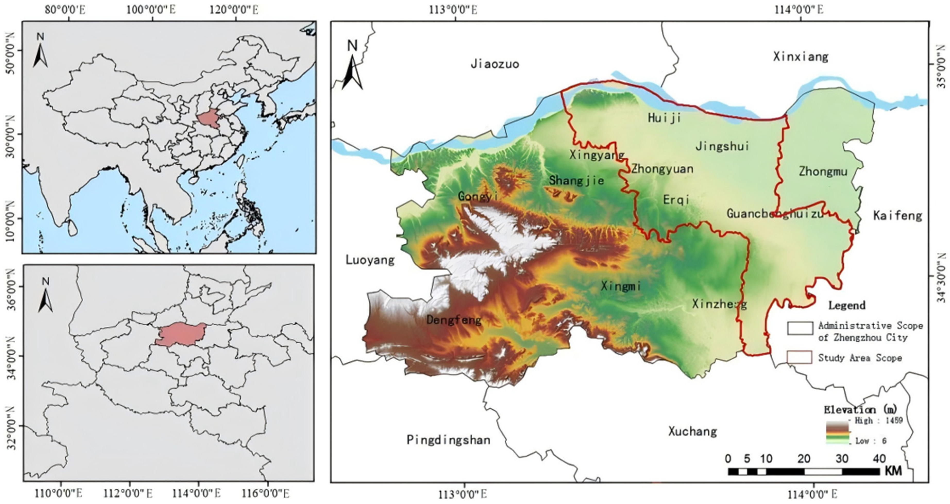
Zhengzhou City is located in the central part of Henan Province. It is a core city of the Central Plains Urban Agglomeration and one of the national central cities, with geographical coordinates approximately between 34°16′–34°58′ N and 112°42′–114°14′ E. This study selects the main urban area of Zhengzhou as the study area, covering the core built-up zones including Jinshui District, Zhongyuan District, Erqi District, Guancheng Hui District, Huiji District, Zhengdong New District, and Zhengzhou Airport Economy Zone (Figure 1). The regional terrain generally slopes downward from west to east, with a hilly transition zone in the west and the Huanghuai Plain in the east. The climate is a temperate monsoon climate, characterized by high temperatures and abundant rainfall in summer. The average temperature is relatively high from July to August, which is the period when the urban heat island effect is most significant. The LST image data used in this study are derived from Landsat 8 remote sensing images, and the analyses are based on images from August 2015 and August 2024.

2.2. Data Sources

The multi-source data used in this study include: Landsat 8 remote sensing image data obtained from the United States Geological Survey (USGS) EarthExplorer portal [https://earthexplorer.usgs.gov (accessed on 10 April 2025)]. Specifically, we downloaded the Collection 2 Level-2 surface temperature (ST) product for the paths/rows covering the study area. This product provides land surface temperature (LST) at 30 m spatial resolution, derived using a Single-Channel (SC) algorithm with atmospheric compensation based on NCEP reanalysis data. The ST product has been validated against in situ measurements with a typical accuracy of ±2–3 °C for clear-sky conditions [29,30]. Two scenes were selected: 23 August 2015 and 3 August 2024, both with cloud cover <10% and acquired under clear-sky conditions. Land use/land cover (LUCC) data were sourced from the Science Data Center of the Chinese Academy of Sciences [http://westdc.westgis.ac.cn (accessed on 12 April 2025)], with a spatial resolution of 30 m. Digital elevation model (DEM) data were sourced from the Geospatial Data Cloud [http://www.gscloud.cn (accessed on 10 April 2025)], with a spatial resolution of 30 m. The normalized difference vegetation index (NDVI) was obtained from LPDAAC-MOD13Q1 (USGS). The administrative boundary and built-up area boundary of Zhengzhou City were obtained from the Zhengzhou Municipal Bureau of Natural Resources and Planning [https://zrzvhhgi.zhengzhou.gov.cn (accessed on 18 March 2025)] (

Table 1. Datasets used in this study.

Data Type	Temporal Range	Spatial Resolution	Data Source
Landsat8 remote sensing image data	LANDSAT/LC08/C01/T1_SR	30 m	https://earthexplorer.usgs.gov (accessed on 10 April 2025)
LUCC (Land-Use/Cover Change)	2015, 2024	—	http://westdc.westgis.ac.cn (accessed on 12 April 2025)
NDVI (Normalized Difference Vegetation Index)	2015, 2024	250 m	LPDAAC-MOD13Q1 [https://earthexplorer.usgs.gov (accessed on 10 April 2025)]
Digital Elevation Model (DEM)	ASTER GDEM 30 m Elevation Data	30 m	http://www.gscloud.cn (accessed on 10 April 2025)
Built-up Area Boundary of Zhengzhou City	2015, 2024	Shapefile format	https://zrzvhhgi.zhengzhou.gov.cn (accessed on 18 March 2025)

) [31].

In this study, strict data screening is implemented to minimize the interference of meteorological and climatic variations on the accurate assessment of the urban heat island effect. First, Landsat 8 images from August 2015 and August 2024 are selected as the analysis data [32,33,34]. August is chosen for two reasons: (1) august represents the period of the highest annual temperatures in Zhengzhou, when land surface temperature and the urban heat island effect are most pronounced, allowing for a full characterization of thermal response differences across different land cover types and improving the ability to identify the relationship between landscape patterns and the thermal environment; and (2) selecting the same month for interannual comparison controls the influence of seasonal variation, differences in solar altitude angle, and changes in vegetation phenology on land surface temperature, thereby enhancing data comparability. Furthermore, during 2015–2024, Zhengzhou experienced significant built-up area expansion and land use restructuring; selecting these two time points captures the stage-specific impacts of landscape pattern changes on SUHII in the context of rapid urbanization [35,36,37]. Therefore, this temporal combination ensures adequate expression of the heat island effect while enhancing the reliability of cross-year comparisons. Based on comprehensive considerations, Landsat 8 images acquired on 23 August 2015 and 3 August 2024, are finally selected. The selection of these two specific years (2015 and 2024) is based on three considerations. First, both images have cloud cover below 10% and were acquired in the same month (August), minimizing seasonal and phenological biases and ensuring comparability. Second, 2015 represents the early stage of Zhengzhou’s recent rapid urbanization, while 2024 represents a later stage after a decade of intensive built-up expansion and landscape restructuring, thus providing a meaningful “before–after” contrast. Third, major urban development milestones (e.g., the expansion of Zhengdong New District and the Airport Economy Zone) occurred between these years, making 2015 and 2024 natural breakpoints for assessing landscape–thermal changes [38]. Nevertheless, we acknowledge that using only two time points cannot capture continuous interannual dynamics [39]. After preprocessing, including radiometric calibration, geometric correction, atmospheric correction, and image cropping, the images are used for subsequent evaluation.

3. Methodology

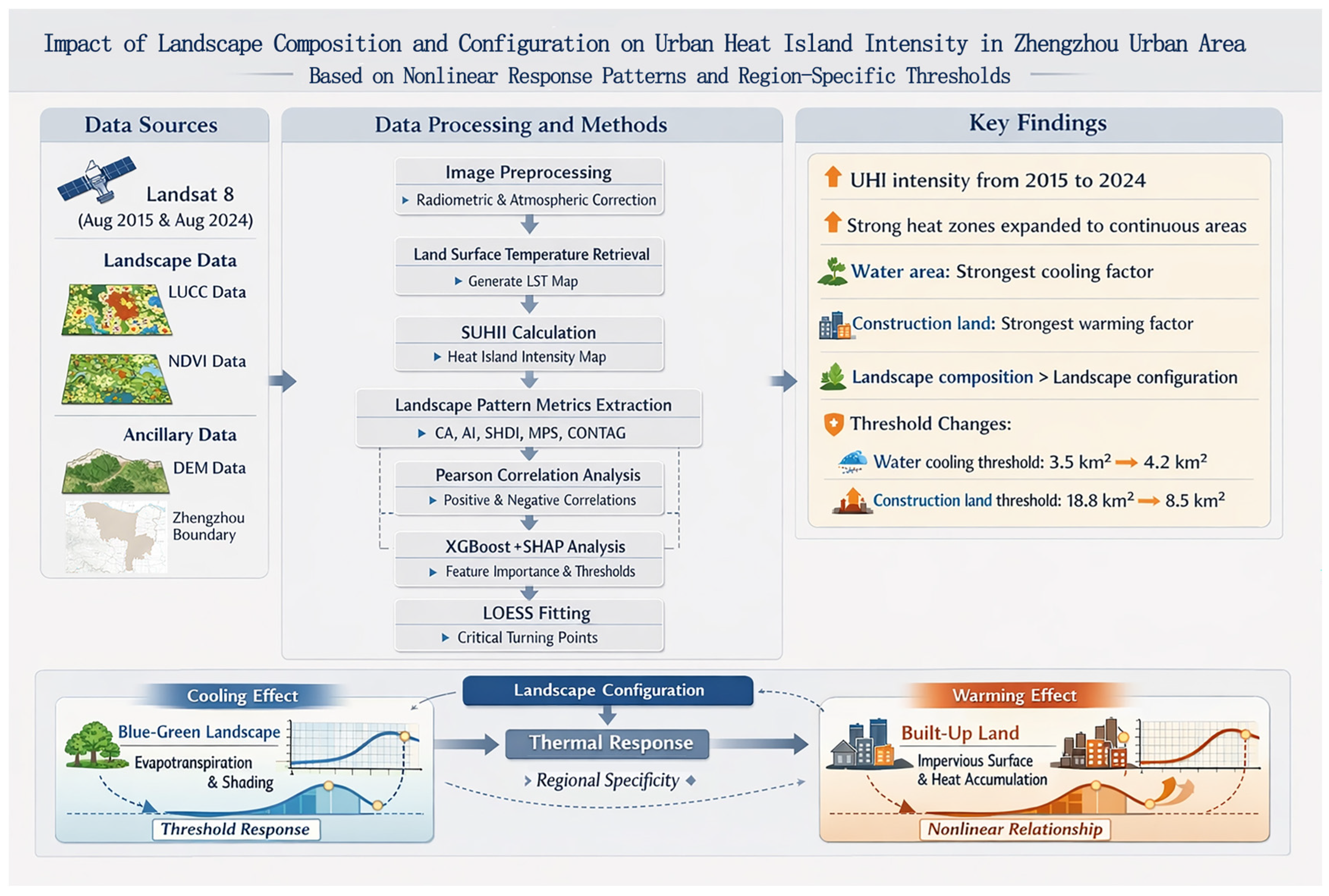
This study comprehensively employs remote sensing retrieval, SUHII quantification, landscape pattern analysis, correlation analysis, and machine learning models to systematically analyze the nonlinear influence mechanism of landscape composition and configuration on SUHII in Zhengzhou. The conceptual framework (Figure 2) proceeds as: landscape indicators → XGBoost prediction of SUHII → SHAP importance and dependence plots → threshold detection → planning implications. This chain makes explicit how machine learning analysis bridges landscape patterns and heat island response.

3.1. Data Preprocessing

Based on the Landsat 8 remote sensing images acquired on 23 August 2015 and August 3, 2024, preprocessing steps including radiometric calibration, geometric correction, atmospheric correction, and image cropping were performed using ENVI 5.6. To reduce the influence of cloud cover, atmospheric conditions, and meteorological fluctuations on land surface temperature retrieval, only images with cloud cover below 10% were strictly selected. Cloud and cloud-shadow pixels were masked using the quality assessment band. Valid pixel coverage was 93.2% (2015) and 91.7% (2024); missing pixels were not imputed to avoid artificial autocorrelation. Furthermore, using the administrative boundary and built-up area of Zhengzhou City, the images were uniformly projected, spatially registered, and cropped to ensure consistent spatial resolution, coordinate system, and study area extent across different years. To enhance comparability in subsequent landscape pattern analysis and machine learning modeling, all raster data were uniformly resampled to a spatial resolution of 30 m.

3.2. Land Surface Temperature Retrieval

Quantitative retrieval of land surface temperature (LST) is a prerequisite for studying the urban heat island effect. Currently, the main methods for retrieving LST from remote sensing data include the radiative transfer equation (RTE) algorithm, as well as the single-window and split-window algorithms, all of which serve as atmospheric correction methods [40,41]. However, due to the presence of significant missing values in the study area, this study adopts the RTE algorithm for LST retrieval. The rainy season in the study area typically occurs between July and September; therefore, this study uses Landsat 8 data from 23 August 2015 and 3 August 2024 for land surface temperature retrieval. The retrieval process includes calculating thermal infrared radiation, determining land surface emissivity, calculating black-body radiation, and calculating land surface temperature [42,43].

The thermal infrared radiation value received by the satellite sensor is calculated using the following formula:

$${\mathrm{L}}_{\mathsf{\lambda }}=[\mathsf{\epsilon }\cdot \mathrm{B}({\mathrm{T}}_{\mathrm{s}})+(1-\mathsf{\epsilon })\cdot \mathrm{L}\downarrow ]\mathsf{\tau }+\mathrm{L}\uparrow$$

(1)

Let $L_{\lambda }$ represent the thermal infrared band radiance received by the satellite sensor, $\epsilon$the land surface emissivity, $T_s$ the actual land surface temperature, $B\left(T_s\right)$ the black-body radiance at the land surface temperature$T_{\mathrm{s}}$, $\tau$the atmospheric transmittance in the thermal infrared band, and $L\downarrow$ and $L\downarrow$ the downward and upward atmospheric radiance, respectively, with units in $\mathrm{W}\cdot {\mathrm{m}}^{-2}\cdot \mathrm{s}{\mathrm{r}}^{-1}\cdot \mathsf{\mu }{\mathrm{m}}^{-1}$.

Land surface emissivity is calculated using the following formula:

$${\mathrm{P}}_{\mathrm{v}}={\displaystyle \frac{\mathrm{N}\mathrm{D}\mathrm{V}\mathrm{I}-\mathrm{c}}{\mathrm{N}\mathrm{D}\mathrm{V}{\mathrm{I}}_{\mathrm{v}}-\mathrm{N}\mathrm{D}\mathrm{V}{\mathrm{I}}_{\mathrm{s}}}}$$

(2)

$$\mathsf{\epsilon }=0.004{\mathrm{P}}_{\mathsf{\nu }}+0.986$$

(3)

In this formula, $P_v$ represents the fractional vegetation cover, $NDVI$ is the normalized difference vegetation index, $NDV{I}_s$ is the $NDVI$ value of bare soil or areas with no vegetation cover, and $NDV{I}_v$ is the NDVI value of areas fully covered by vegetation. Generally, when $NDVI$ > 0.7, $P_v$ = 1; when $NDVI$ < 0.05, $P_v$ = 0. Combining Equations (1) and (2), the black-body radiance in the thermal infrared band is calculated as follows:

$$\mathrm{B}({\mathrm{T}}_{\mathrm{s}})={\displaystyle \frac{{\mathrm{L}}_{\mathsf{\lambda }}-{\mathrm{L}}^{\uparrow }-\mathsf{\tau }\cdot (1-\mathsf{\epsilon })\cdot {\mathrm{L}}^{\downarrow }}{\mathsf{\tau }\cdot \mathsf{\epsilon }}}$$

(4)

Finally, the land surface temperature (LST) is obtained, and its calculation formula is as follows:

$$\mathrm{L}\mathrm{S}\mathrm{T}={\displaystyle \frac{1321.08}{\mathrm{a}\mathrm{l}\mathrm{o}\mathrm{g}(774.89/\mathrm{b}10+1)}}-273.15$$

(5)

where $LST$ is the land surface temperature (unit: °C); b10 is the black-body radiance at the same temperature (unit: W/(m²·sr)).

3.3. Calculation of Surface Urban SUHII

Urban land surface temperature itself is strongly influenced by multi-scale climatic fluctuations, and the interannual variation in its absolute value cannot adequately represent the actual impact of urban construction. Therefore, this study uses the SUHII, which characterizes the temperature difference between urban and rural areas, to conduct the assessment. The calculation formula is as follows:

$$\mathrm{S}\mathrm{U}{\mathrm{H}\mathrm{I}}_{\mathrm{i}}=\mathrm{L}\mathrm{S}\mathrm{T}{\mathrm{U}}_{\mathrm{i}}-\mathrm{L}\mathrm{S}{\mathrm{T}}_{\mathrm{S}}$$

where $SU{HI}_i$ represents the SUHII of the $i$ pixel in the urban area (unit: °C), $LST{U}_i$ represents the actual land surface temperature of the $i$ pixel in the urban area, and $LS{T}_S$ represents the mean land surface temperature of the rural reference area. The selection of the rural reference area also affects the accuracy of thermal environment assessment. For example, development and construction activities may raise the temperature in rural areas, leading to an underestimation of SUHII; conversely, afforestation may cool rural areas, resulting in an overestimation of SUHII. The rural reference area was defined as the mean LST of all non-built-up, non-water pixels located outside the urban boundary within a 5 km buffer. This definition was used consistently for both 2015 and 2024.

3.4. Extraction of Landscape Composition and Configuration Indices

To quantitatively characterize the compositional structure and spatial configuration of different landscape types, this study extracts multi-dimensional landscape pattern indices based on land use data using the Fragstats 4.2 platform, and constructs a landscape indicator database at a 500 m grid scale. The 500 m grid balances spatial detail and the stability of landscape indices, and is well matched to the typical urban functional units and block scales in Zhengzhou. Following standard landscape ecology terminology [44], we distinguish between landscape composition and landscape configuration. Landscape composition refers to the area and abundance of different land cover types, quantified by the patch area (CA) of green space, water bodies, and built-up land. Landscape configuration refers to the spatial arrangement, shape, and aggregation of patches, quantified by two subsets of metrics: Class-level configurational metrics: aggregation index (AI) for green space, water body, and built-up land. Landscape-level configurational metrics: Shannon’s diversity index (SHDI), mean patch area (MPS), and contagion index (CONTAG). Accordingly, the selected indicators are organized as follows: Compositional indicators (CA): green space CA, water body CA, and built-up land CA. Configurational indicators (AI, SHDI, MPS, CONTAG): green space AI, water body AI, built-up land AI, SHDI, MPS, CONTAG. Among these, CA reflects the size characteristics of different landscape types; AI measures the degree of aggregation among patches of the same type; SHDI characterizes the complexity and diversity of land cover types; MPS reflects the average patch size; and CONTAG indicates the overall connectivity and clumping of the landscape.

3.5. Correlation Analysis Between Landscape Indicators and SUHII

To preliminarily identify the relationship between landscape composition and configuration and SUHII, this study employs the Pearson correlation analysis method to measure the linear relationship between each landscape indicator and SUHII in 2015 and 2024. The Pearson correlation coefficient reflects the direction (positive or negative) and strength of the relationship between variables, and its calculation formula is as follows:

$$r={\displaystyle \frac{\sum (x_i-\bar{x}\left)\right(y_i-\bar{y})}{\sqrt{\sum (x_i-\bar{x}{)}^2}\sum (y_i-\bar{y}{)}^2}}$$

where $\mathrm{r}$ is the Pearson correlation coefficient, ranging from −1 to 1. When r > 0, it indicates a positive correlation; when r < 0, it indicates a negative correlation. The larger the absolute value, the stronger the correlation. Meanwhile, the reliability of the correlation is assessed through significance testing: when p < 0.05, the correlation between variables is considered statistically significant; when p < 0.01, the correlation is considered extremely significant.

3.6. Identification of Driving Mechanisms and Nonlinear Thresholds Using XGBoost-SHAP

Pearson correlation analysis can only capture linear relationships between variables, whereas the influence of landscape composition and configuration on SUHII often involves complex nonlinear effects and interactions. Therefore, this study further introduces the XGBoost machine learning model and the SHAP interpretability method to deeply identify the driving mechanisms of landscape composition and configuration [45,46]. Compared with traditional statistical approaches, XGBoost offers several advantages: (1) it inherently handles nonlinearity and non-normal distributions; (2) it captures interactions among landscape metrics without explicit specification; (3) it provides feature importance rankings based on marginal contributions; and (4) when combined with SHAP dependence plots, it enables the identification of critical thresholds where the effect of a landscape factor changes sign or magnitude. Here, SUHII is taken as the dependent variable, and each landscape pattern indicator is used as an independent variable to construct a regression model. The coefficient of determination (R²) and root mean square error (RMSE) are used to evaluate the model fitting performance. On this basis, the SHAP (Shapley Additive Explanations) method is introduced to interpret the model outputs. SHAP values quantify the marginal contribution of each landscape indicator to the predicted SUHII; the larger the absolute value, the higher the importance of that variable [47]. Furthermore, by integrating SHAP summary plots, SHAP dependence plots, and spatial mapping results, the following objectives are achieved: identifying the key landscape factors influencing SUHII; revealing the warming or cooling direction of different landscape indicators on SUHII; and analyzing the nonlinear response relationships of each landscape indicator.

Based on SHAP dependence plots combined with locally weighted scatterplot smoothing (LOESS, span = 0.5), we identified thresholds as the zero-crossing points where the smoothed SHAP value changes sign (e.g., from negative to positive, indicating a shift from cooling to warming). For each threshold, we recorded the highest$x$with a negative raw SHAP value and the lowest $x$ with a positive raw SHAP value in the immediate vicinity of the zero-crossing (within ±10% of the data range). The interval between these two values is reported as the empirical uncertainty range, while the zero-crossing point serves as the point estimate. These ranges are descriptive measures of the local dispersion of SHAP values and do not represent formal confidence intervals. For indicators with multiple zero-crossings, each threshold is identified and reported separately. The resulting thresholds and their uncertainty ranges for all indicators in 2015 and 2024 are provided in Appendix B 

Table A2. Empirical uncertainty ranges for key landscape indicators derived from SHAP dependence plots (2015).

Indicator	Unit	Threshold Point Estimate	Empirical Uncertainty Range [Last Negative SHAP, First Positive SHAP]
CONTAG (multiple thresholds)	%	14.6	[12.0, 16.8]
	%	49.6	[47.0, 52.1]
	%	82.4	[80.0, 84.9]
	%	97.0	[95.0, 98.8]
SHDI (multiple thresholds)	–	0.20	[0.15, 0.26]
	–	0.70	[0.62, 0.78]
	–	1.10	[1.02, 1.19]
	–	1.30	[1.22, 1.37]
Green Space CA	km2	1.9	[1.5, 2.1]
	km2	2.6	[2.2, 3.0]
Green Space AI	%	68.0	[65.0, 70.4]
	%	72.3	[70.0, 74.6]
	%	95.7	[93.0, 97.9]
Water CA	km2	2.5	[2.1, 2.9]
	km2	3.5	[3.1, 3.9]
Water AI	%	66.8	[63.5, 69.1]
	%	71.7	[69.2, 73.9]
Construction Land CA	km2	15.1	[14.0, 16.3]
	km2	17.4	[16.2, 18.2]
	km2	18.8	[17.9, 19.7]
Construction Land AI	%	80.0	[77.0, 82.3]
	%	97.7	[95.1, 99.2]
MPS	km2	3.6	[3.0, 4.1]

and

Table A3. Empirical uncertainty ranges for key landscape indicators derived from SHAP dependence plots (2024).

Indicator	Unit	Threshold Point Estimate	Empirical Uncertainty Range [Last Negative SHAP, First Positive SHAP]
CONTAG (multiple thresholds)	%	16.1	[13.8, 18.3]
	%	28.9	[26.3, 31.2]
	%	35.2	[32.5, 37.5]
	%	82.1	[79.4, 84.5]
SHDI (multiple thresholds)	–	0.60	[0.53, 0.67]
	–	1.00	[0.91, 1.08]
	–	1.20	[1.12, 1.28]
Green Space CA	km2	1.9	[1.4, 2.2]
	km2	2.3	[1.9, 2.7]
Green Space AI	%	69.5	[66.6, 71.9]
	%	71.8	[69.4, 74.1]
Water CA	km2	2.7	[2.2, 3.1]
	km2	4.2	[3.7, 4.7]
Water AI	%	74.3	[71.1, 76.6]
	%	78.4	[75.5, 80.8]
Construction Land CA	km2	8.5	[7.2, 9.7]
Construction Land AI	%	68.3	[65.2, 70.6]
	%	98.5	[95.8, 99.8]
MPS	km2	3.9	[3.2, 4.4]

Note: The empirical uncertainty range for each threshold is defined as the interval from the last negative SHAP value to the first positive SHAP value observed in the SHAP dependence plot in the immediate vicinity of the zero crossing. The point estimate is the zero-crossing value (midpoint of the interval when multiple crossings exist, or the reported threshold from the LOESS curve). These ranges are descriptive measures of the local dispersion of SHAP values around zero and do not represent formal confidence intervals.

.

It is important to clarify that the empirical uncertainty ranges reported in Appendix B are descriptive measures of the local dispersion of raw SHAP values around the zero-crossing of the LOESS-smoothed curve. They are intended to illustrate the sensitivity of the response curves to local data variability, rather than to serve as formal confidence intervals (e.g., bootstrapped or holdout-based intervals). Therefore, throughout this manuscript, we refer to these values as indicative benchmarks or exploratory thresholds, not as statistically confirmed fixed cut-off values.

This procedure yields both a point estimate and a range for each threshold, reflecting the nonlinear characteristics of landscape composition and configuration impacts on the thermal environment and providing quantitative references for the allocation of urban blue–green spaces, control of built-up area scale, and thermal environment optimization.

To ensure model robustness, the samples were divided into training and testing sets at a ratio of 7:3. The XGBoost model was initially trained using default parameters (n_estimators = 100, max_depth = 6, learning_rate = 0.3) as a baseline. The R² values for 2015 were 0.73 (training) and 0.79 (testing); for 2024, 0.80 (training) and 0.82 (testing), indicating no severe overfitting. A dedicated hyperparameter sensitivity analysis is presented in Section 3.7. Finally, this study focuses on identifying the threshold ranges of key indicators such as water body area, built-up area, green space area, and aggregation index, and compares their changes between 2015 and 2024, thereby comparing the thresholds between 2015 and 2024 in the context of rapid urbanization.

Importantly, the thresholds reported for 2015 and 2024 are derived from two independent cross-sectional models. The differences between the two years indicate a change in the empirical relationship between landscape factors and SUHII, but they do not directly measure a temporal trend or a dynamic “shift” of thresholds over time. Establishing whether these differences represent a monotonic trajectory or a fluctuating pattern would require data from multiple intermediate years. Therefore, our comparison is interpreted as a difference between two urbanization stages, not as evidence of continuous evolution. It is also important to note that the thresholds identified through this procedure are exploratory in nature. They are derived from SHAP dependence plots combined with LOESS, and the uncertainty ranges reflect local dispersion of raw SHAP values around the zero-crossing rather than statistically validated confidence intervals (e.g., bootstrapped or holdout-based intervals). Therefore, these thresholds should be interpreted as indicative values that reveal nonlinear response patterns, not as statistically confirmed fixed critical values. Future studies with larger sample sizes or formal uncertainty quantification (e.g., bootstrap over grids) are needed to validate their robustness.

3.7. Hyperparameter Sensitivity Analysis

To evaluate whether our results are sensitive to the choice of XGBoost hyperparameters, we compared the default configuration (n_estimators = 100, max_depth = 6, learning_rate = 0.3) against two alternative settings: (i) a more conservative setting (n_estimators = 150, max_depth = 4, learning_rate = 0.1) that reduces model complexity, and (ii) a more complex setting (n_estimators = 80, max_depth = 8, learning_rate = 0.5) that allows deeper interactions. For each setting, we retrained the model and recalculated SHAP feature importance and the key thresholds (water body cooling threshold and built-up warming threshold).

The results are summarized in Appendix A 

Table A1. Sensitivity of SHAP feature importance and key thresholds to XGBoost hyperparameters.

Hyperparameter Set	Top 3 Features (SHAP Rank)	Water Threshold (2015)	Water Threshold (2024)	Built-Up Threshold (2015)	Built-Up Threshold (2024)
Default (d = 6, lr = 0.3, n = 100)	waterCA > builtCA built AI	3.5 km2	4.2 km2	18.8 km2	8.5 km2
Conservative (d = 4, lr = 0.1, n = 150)	waterCA > builtCA built AI	3.4 km2	4.0 km2	19.2 km2	8.8 km2
Complex (d = 8, lr = 0.5, n = 80)	waterCA > builtCA > built AI	3.6 km2	4.3 km2	18.5 km2	8.3 km2

Note: d = max_depth, lr = learning_rate, n = n_estimators.

. Across all three configurations, the top three features by SHAP importance were consistently water body CA, built-up CA, and built-up AI, in the same order. The estimated cooling threshold for water body area varied by at most ±0.2 km² (2015) and ±0.3 km² (2024); the warming threshold for built-up area varied by ±0.7 km² (2015) and ±0.5 km² (2024). These small variations suggest that our core findings are robust to reasonable changes in hyperparameters, although a full grid search or Bayesian optimization would be more exhaustive.

4. Cross-Stage Comparison of SUHII Between 2015 and 2024

4.1. Overall Changes in SUHII

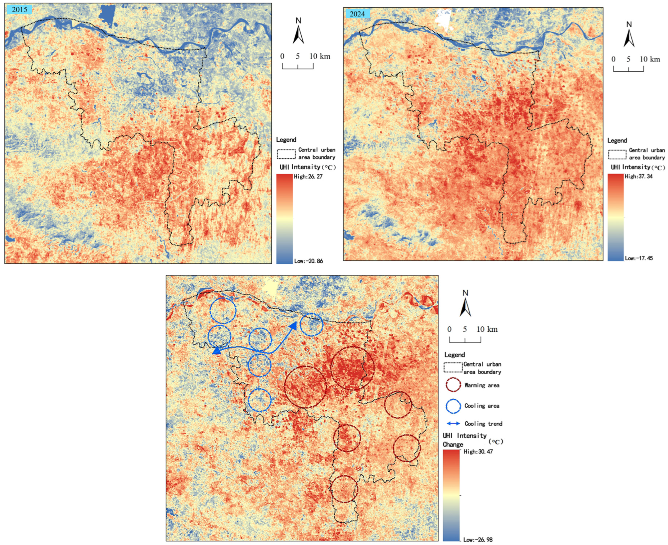
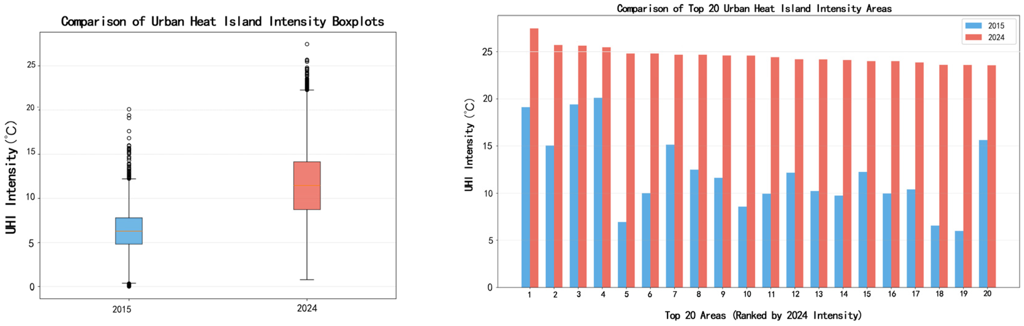
Between 2015 and 2024, the surface urban SUHII in the built-up area of Zhengzhou was substantially higher in 2024 than in 2015. The average SUHII was 6.22 °C in 2015 and 11.51 °C in 2024, indicating a marked difference in the thermal environment between the two years. (Figure 3 and Figure 4). In terms of the intensity hierarchy, the heat island was dominated by low and moderate levels in 2015, with high-level heat islands scattered sporadically. In contrast, the proportions of strong heat islands (16–20 °C) and extremely strong heat island (≥20 °C) areas were substantially larger in 2024. (

Table 2. Core statistics of SUHII in the main urban area of Zhengzhou.

Year	Total Grids	Mean (°C)	Standard Deviation	Number of Strong UHI Grids	Proportion of Strong UHI Grids (%)	Number of Extreme UHI Grids	Proportion of Extreme UHI Grids (%)
2015	14,688	6.22	2.20	326	2.22	18	0.12
2024	14,688	11.51	2.93	3842	26.16	344	2.34

Note: Strong UHI is defined as 16 °C ≤ SUHII < 20 °C; extreme UHI is defined as SUHII ≥ 20 °C. These thresholds are consistent with the intensity classification used in Section 4.1.

)These results indicate that Zhengzhou’s thermal environment in 2024 differed from that in 2015, shifting from a stage of “localized high-temperature patch distribution” to a stage of “continuous high-temperature expansion.” From the perspective of the intensity hierarchy, the heat island was mainly characterized by low and moderate intensity in 2015, with high-level heat islands scattered sporadically; by 2024, strong heat island areas had expanded from localized patches to contiguous zones, forming a continuous distribution pattern. Spatially, high-temperature areas have expanded mainly from the central urban area toward Zhengdong New District, the Airport Economy Zone, and peripheral industrial parks, gradually forming multiple continuous high-temperature core areas, spreading in a belt-like pattern along transportation corridors and concentrated built-up areas.

4.2. Spatial Structural Differences in the Urban Heat Island Between 2015 and 2024

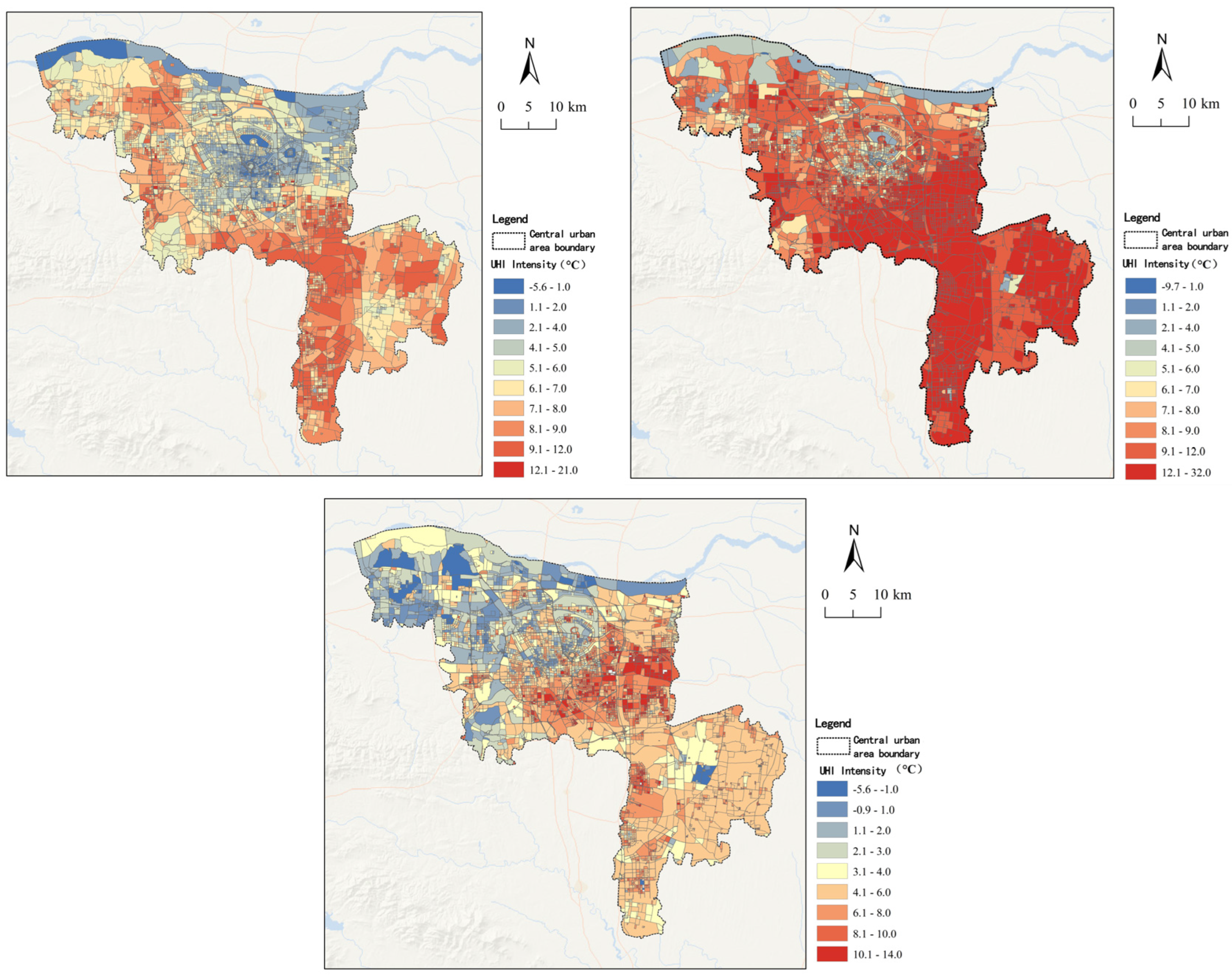
Comparison of spatial patterns shows that in 2015, high-level heat islands were mainly concentrated in the core built-up area of the central city, exhibiting a punctate or small-patch distribution. By 2024, areas of strong and extremely strong heat islands had significantly expanded outward toward the urban periphery (Figure 5). This expansion trend is highly consistent with the spatial expansion direction of the built-up area, presenting a typical “outward-expansion pattern of heat island intensification.” In the newly developed peripheral areas, the rapid increase in built-up land, the rise in impervious surface proportion, and the compression of ecological space have led to the outward spread of high-temperature patches along urban development axes. Meanwhile, the spatial pattern of the heat island in 2024 exhibits the following characteristics: enhanced connectivity of high-temperature areas; expansion of the heat island core area; gradual disappearance of marginal transition zones; and a shift in the temperature gradient from a “center–suburb declining pattern” to a “multi-core superimposed pattern.” This comparison suggests that urban spatial expansion between 2015 and 2024 was associated with both higher temperature levels and a reorganized spatial pattern of the heat island.

5. Driving Mechanisms of Landscape Composition and Configuration and SUHII

5.1. Linear Correlation Characteristics

The results show a clear differentiation between cooling factors (green space, water, SHDI) and warming factors (built-up area and its aggregation index), with pattern-related indicators (MPS, CONTAG) showing no significant linear correlation. To control false positives due to multiple comparisons, the Bonferroni correction (α′ = 0.05/18 ≈ 0.0028) was applied. All core variables discussed (water body CA, built-up CA, built-up AI, SHDI, green space CA) remained significant (p < 0.001), confirming the robustness of the findings.

5.1.1. Cooling Factors with Significant Negative Correlations

Green space patch area, water body patch area, and SHDI showed significant negative correlations with SUHII in both years. Among these, the water body patch area was the most prominent cooling factor. This is attributed to the high specific heat capacity and strong evaporative characteristics of water bodies, which consume substantial sensible heat through latent heat flux, resulting in a more stable and pronounced cooling effect compared to green spaces. Green space patch area exhibited a moderate negative correlation with SUHII in both years. Green spaces reduce land surface temperature through vegetation transpiration and canopy shading, but their cooling effect is constrained by vegetation coverage and community structure. Shannon’s diversity index, which reflects the diversity of landscape composition, showed a significant negative correlation with SUHII in both years, implying that a landscape structure composed of diverse land cover types can avoid the concentration of heat sources, form a heterogeneous thermal environment, and thereby weaken the SUHII.

5.1.2. Warming Factors with Significant Positive Correlations

Built-up land patch area and built-up land aggregation index are the primary warming factors, showing significant positive correlations with SUHII in both years. Built-up land patch area was the strongest warming factor in 2015 and still maintained a moderately strong positive correlation in 2024. The large-scale expansion of built-up land leads to a substantial increase in the proportion of impervious surfaces (e.g., concrete, asphalt). The built-up land aggregation index is also significantly positively correlated with SUHII, because the high aggregation of built-up land forms continuous “hot patches,” hindering the dispersion and exchange of heat between urban and rural areas and exacerbating heat accumulation.

5.2. Differences Between 2015 and 2024

From 2015 to 2024, the direction of the correlations between each landscape indicator and SUHII in Zhengzhou remained unchanged (negative correlations for cooling factors, positive correlations for warming factors), indicating that the core driving logic of the urban heat island effect—namely “cooling by blue–green spaces and warming by built-up land”—remains stable during rapid urbanization. However, the magnitudes of the correlation coefficients for all types of indicators weakened to some extent. The differences between the two study years and the driving causes are as follows (Figure 6):

5.2.1. Spatial Distribution Characteristics of Landscape Composition and Configuration

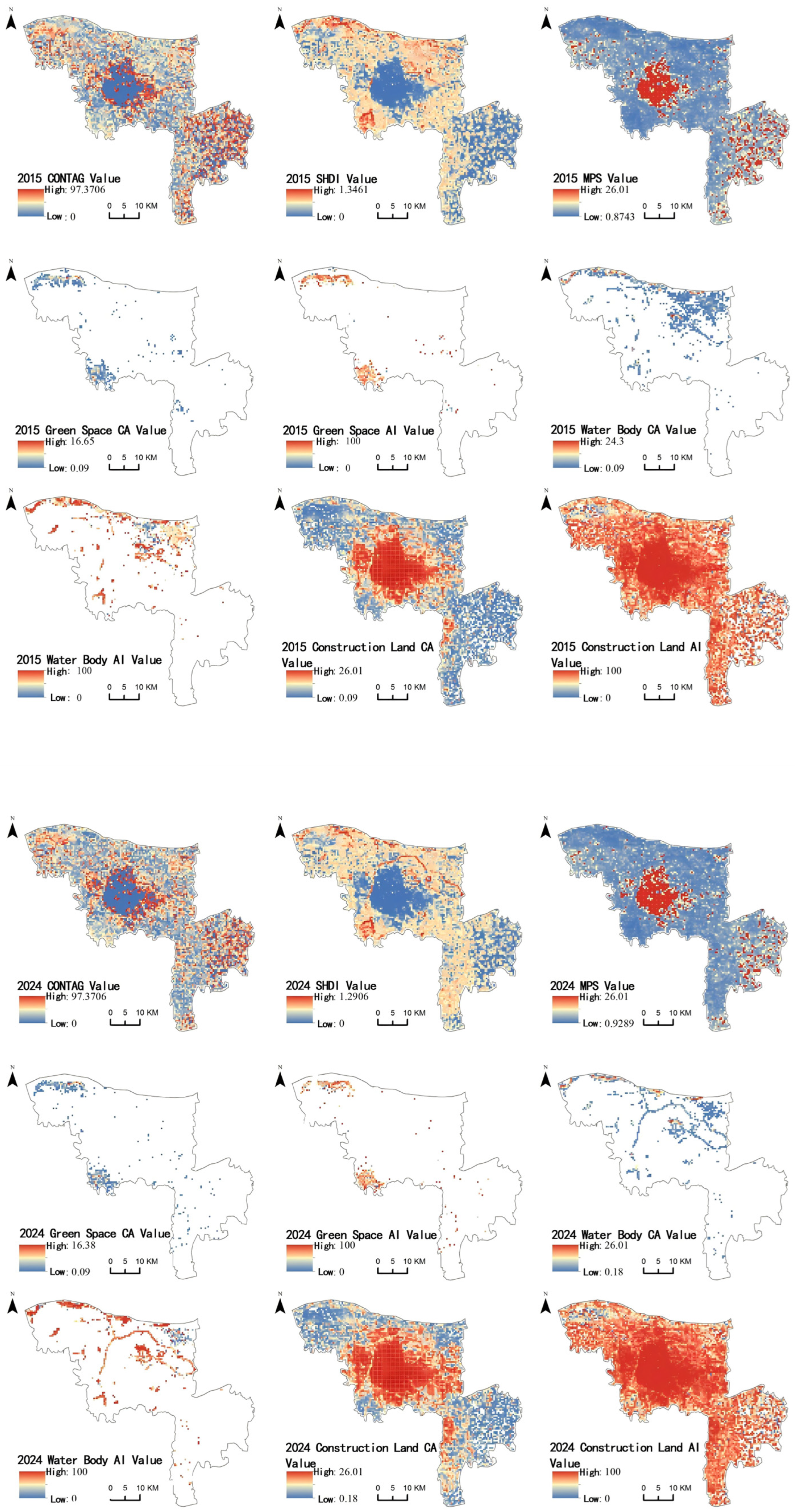
From 2015 to 2024, the landscape pattern indices in the main urban area of Zhengzhou exhibited significant spatial heterogeneity and clear changes between 2015 and 2024 (Figure 5). At the overall landscape level, the high-value areas of CONTAG (contagion index) extended from the central urban area toward the periphery with urban expansion; the high-value areas of SHDI (Shannon’s diversity index) spread into urban–rural transition zones; and the high-value areas of MPS (mean patch area) expanded substantially. These trends collectively reflect the dominant trend toward contiguous and large-scale urban built-up land, with landscape types in the central urban area tending to become more homogeneous, while landscape complexity was higher in peripheral areas. At the ecological landscape level, high-value areas of green space and water body CA (patch area) and AI (aggregation index) continuously shrank, remaining only scattered in the outer suburbs and along the Yellow River. Ecological spaces were persistently encroached upon by built-up land, resulting in decreased connectivity and increased fragmentation. At the built-up land level, high-value areas of its CA and AI expanded from the core area to the entire periphery, with aggregation and scale increasing simultaneously, making built-up land the dominant type shaping the urban landscape pattern. Overall, during the study period, the landscape pattern of Zhengzhou exhibited an evolutionary characteristic of “contiguous expansion of built-up land and shrinkage and fragmentation of ecological space.” The spatial differentiation of various indices was highly coupled with the distribution of SUHII, providing a clear pattern basis for analyzing the driving mechanisms of the thermal environment.

5.2.2. Weakening of the Cooling Effect of Blue–Green Spaces

From 2015 to 2024, the Pearson correlation coefficients of water body area and green space area with SUHII decreased, and the negative correlation of Shannon’s diversity index weakened from moderate to weak. This attenuation of the cooling effect of blue–green spaces can be attributed to four factors. First, blue–green space fragmentation intensified. The rapid expansion of built-up land encroached upon and fragmented large areas of green space and water bodies, reducing their effective connected area. Second, the ecological functions of blue–green spaces have degraded. Many urban green spaces are dominated by planted vegetation with low transpiration efficiency, while some water bodies suffer from reduced evaporation capacity due to urban pollution, both diminishing cooling potential. Third, statistical artifacts arising from increased nonlinearity and reduced variance. The Pearson coefficient for water body CA fell from −0.589 in 2015 to −0.478 in 2024. This decline does not indicate a true weakening of the cooling effect; instead, it reflects (a) an increasingly nonlinear relationship between water body area and SUHII, which linear correlation cannot fully capture; and (b) a reduction in spatial variance of water body area across grids (SD decreased from 1.42 km² to 0.96 km²), which constrains the correlation coefficient. Notably, XGBoost-SHAP analysis confirmed that water body area remained the most important cooling factor in 2024, indicating its regulatory role did not truly diminish. This attenuation of the cooling effect of blue–green spaces can be attributed to four factors.

5.2.3. Weakening of the Marginal Warming Effect of Built-Up Land but Enhanced Overall Warming Contribution

The correlation coefficients of built-up land patch area and built-up land aggregation index with SUHII (

Table 3. Correlation analysis results between SUHII and landscape variables in 2015.

Variable 1	Variable 2	Correlation Coefficient	p-Value	Significance Level	Relationship Description
UHI Intensity	2015 Green Space CA	−0.523	0.018	p < 0.05 (significant)	Moderate negative correlation: the larger the Green Space CA, the lower the UHI Intensity
UHI Intensity	2015 Green Space AI	0.187	0.382	p > 0.05 (not significant)	No significant correlation
UHI Intensity	2015 Construction Land AI	0.671	0.002	p < 0.01 (highly significant)	Strong positive correlation: the larger the Construction Land AI, the higher the UHI Intensity
UHI Intensity	2015SHDI	−0.415	0.043	p < 0.05 (significant)	Moderate negative correlation: the larger the SHDI, the lower the UHI Intensity
UHI Intensity	2015 Construction Land CA	0.724	0.001	p < 0.01 (highly significant)	Strong positive correlation: the larger the Construction Land CA, the higher the UHI Intensity
UHI Intensity	2015MPS	−0.296	0.175	p > 0.05 (not significant)	No significant correlation
UHI Intensity	2015CONTAG	0.352	0.081	p > 0.05 (not significant)	No significant correlation
UHI Intensity	2015 Water Body CA	−0.589	0.009	p < 0.01 (highly significant)	Strong negative correlation: the larger the Water Body CA, the lower the UHI Intensity
UHI Intensity	2015 Water Body AI	−0.153	0.467	p > 0.05 (not significant)	No significant correlation

Note: After Bonferroni correction for 18 tests (α′ = 0.0028), all correlations marked as significant in the table remain significant (p < 0.001).

and

Table 4. Correlation analysis results between SUHII and landscape variables in 2024.

Variable 1	Variable 2	Correlation Coefficient	p-Value	Significance Level	Relationship Description
UHI Intensity	2024 Green Space CA	−0.387	0.0012	p < 0.01 (Highly significant)	Moderate negative correlation: higher Green Space CA corresponds to lower UHI Intensity
UHI Intensity	2024 Green Space AI	0.125	0.3187	p > 0.05 (Not significant)	No significant correlation
UHI Intensity	2024 Construction Land AI	0.452	0.0003	p < 0.01 (Highly significant)	Moderate positive correlation: higher aggregation of Construction Land corresponds to stronger UHI Intensity
UHI Intensity	2024SHDI	−0.296	0.0158	p < 0.05 (Significant)	Weak negative correlation: higher landscape diversity corresponds to slightly lower UHI Intensity
UHI Intensity	2024 Construction Land CA	0.513	0.0001	p < 0.01 (Highly significant)	Moderate-strong positive correlation: a larger area of Construction Land corresponds to stronger UHI Intensity
UHI Intensity	2024MPS	−0.087	0.4926	p > 0.05 (Not significant)	No significant correlation
UHI Intensity	2024CONTAG	0.169	0.1935	p > 0.05 (Not significant)	No significant correlation
UHI Intensity	2024 Water Body CA	−0.478	0.0002	p < 0.01 (Highly significant)	Moderate negative correlation: a larger area of the water body corresponds to lower UHI Intensity
UHI Intensity	2024 Water Body AI	0.053	0.6742	p > 0.05 (Not significant)	No significant correlation

Note: After Bonferroni correction for 18 tests (α′ = 0.0028), all correlations marked as significant in the table remain significant (p < 0.001).

) decreased from 0.724 and 0.671 in 2015 to 0.513 and 0.452 in 2024, respectively, indicating a significant attenuation of the warming effect of built-up land. The causes of this observed change are not directly identifiable from our dataset. The reduced correlation coefficients should be interpreted with caution; they may be influenced by multiple factors, such as changes in land use policies, urban greening initiatives, or statistical artifacts (e.g., reduced spatial variance). However, confirming any specific causal mechanism would require dedicated data and analysis beyond the scope of this study.

Nevertheless, although the correlation coefficients for built-up land have decreased, this does not mean that the role of built-up land in the heat island effect has weakened; rather, it indicates that the marginal warming effect per unit area of built-up land has decreased. Because the total area of built-up land in Zhengzhou continues to expand, built-up land remains the primary source driving heat island intensification, and thus the overall thermal environment continues to warm significantly.

6. Nonlinear Response and Identification of Key Factors

In this study, with SUHII as the dependent variable, and green space patch area (green space CA), green space aggregation index (green space AI), built-up land patch area (built-up land CA), built-up land aggregation index (built-up land AI), Shannon’s diversity index (SHDI), mean patch area (MPS), contagion index (CONTAG), water body patch area (water body CA), and water body aggregation index (water body AI) as independent variables, an XGBoost machine learning regression model was constructed. This model has a good fitting capability for nonlinear, non-normally distributed geographic data and can effectively handle multicollinearity among indicators. On this basis, the SHAP interpretability method is introduced. The feature importance ranking is determined by calculating the SHAP value of each landscape indicator. SHAP dependence plots are used to characterize the nonlinear response relationships between indicators and SUHII, and the SHAP values are visualized to identify the effect thresholds of key factors.

6.1. SHAP Feature Importance Ranking and Identification of Core Driving Factors

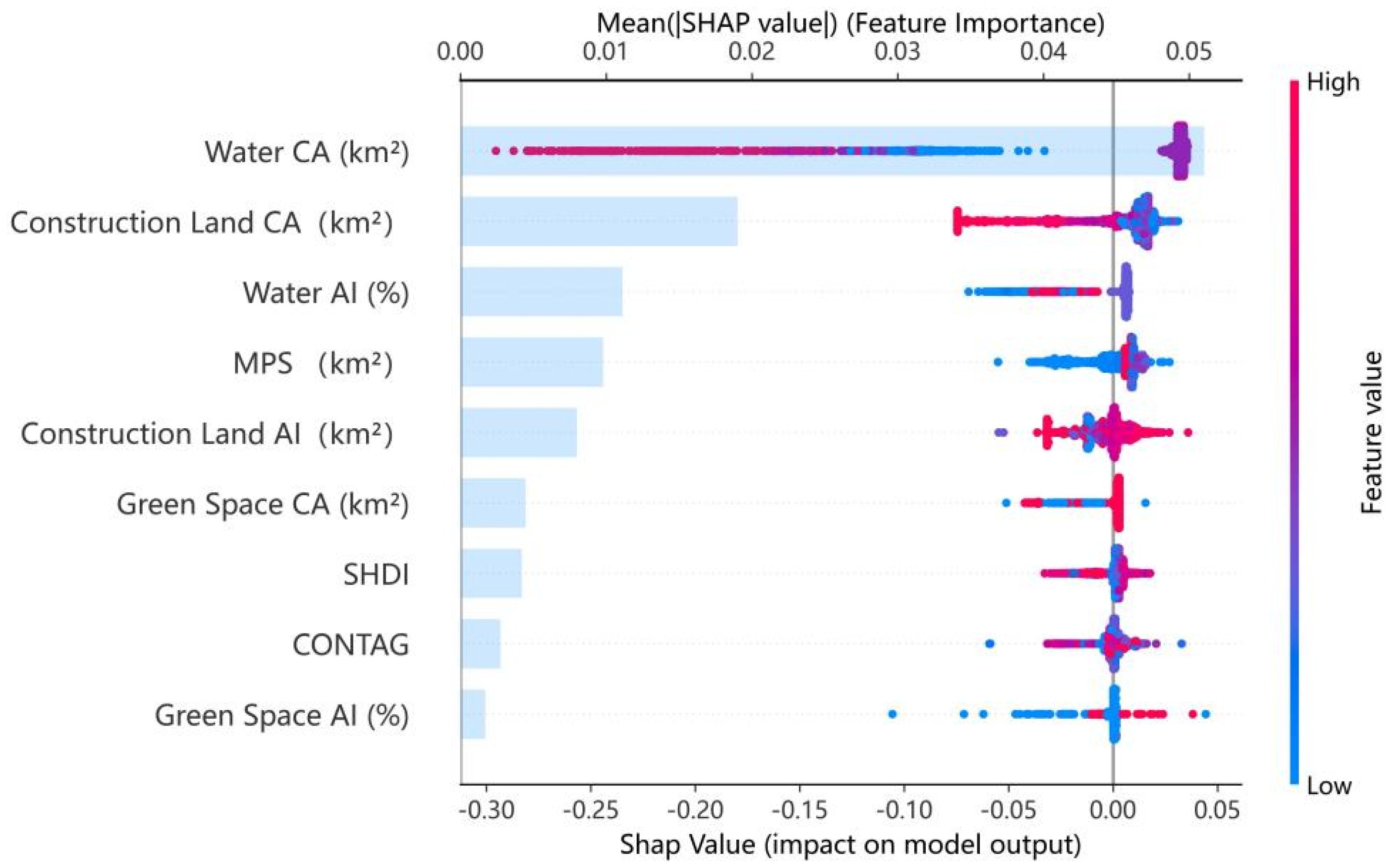
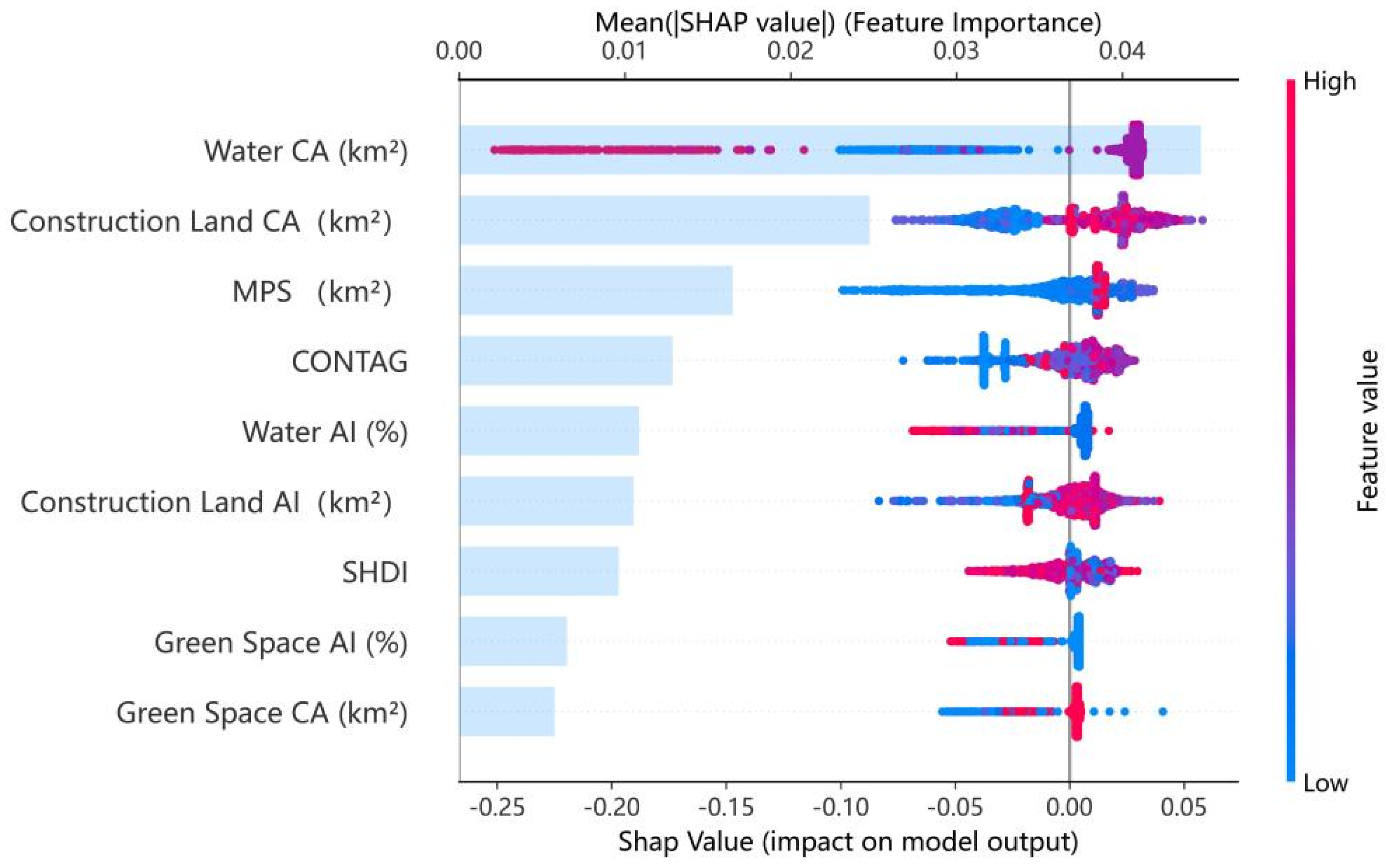
The SHAP value for feature importance represents the average contribution of each landscape indicator to the model output of SUHII. The larger the SHAP value, the stronger the explanatory power and driving effect of that indicator on SUHII (Figure 7 and Figure 8). Water body CA has the highest mean SHAP value in both years (0.42 in 2015, 0.38 in 2024), ranking first among all landscape indicators. This indicates that the water body area is the primary factor regulating SUHII in Zhengzhou, and its core status has not changed over time. Built-up land CA ranks second in SHAP importance (mean SHAP = 0.36 in 2015, 0.31 in 2024). Its contribution to SUHII is primarily positive, confirming its role as the main warming driver. As the main carrier of urban impervious surfaces, the expansion of built-up land area directly determines the heat absorption and heat storage capacity of the urban surface. Its contribution to explaining SUHII is close to that of water body CA, making it the main cause of heat island intensification in Zhengzhou.

6.2. Exploratory Threshold Identification and Indicative Cross-Stage Differences in Key Landscape Factors

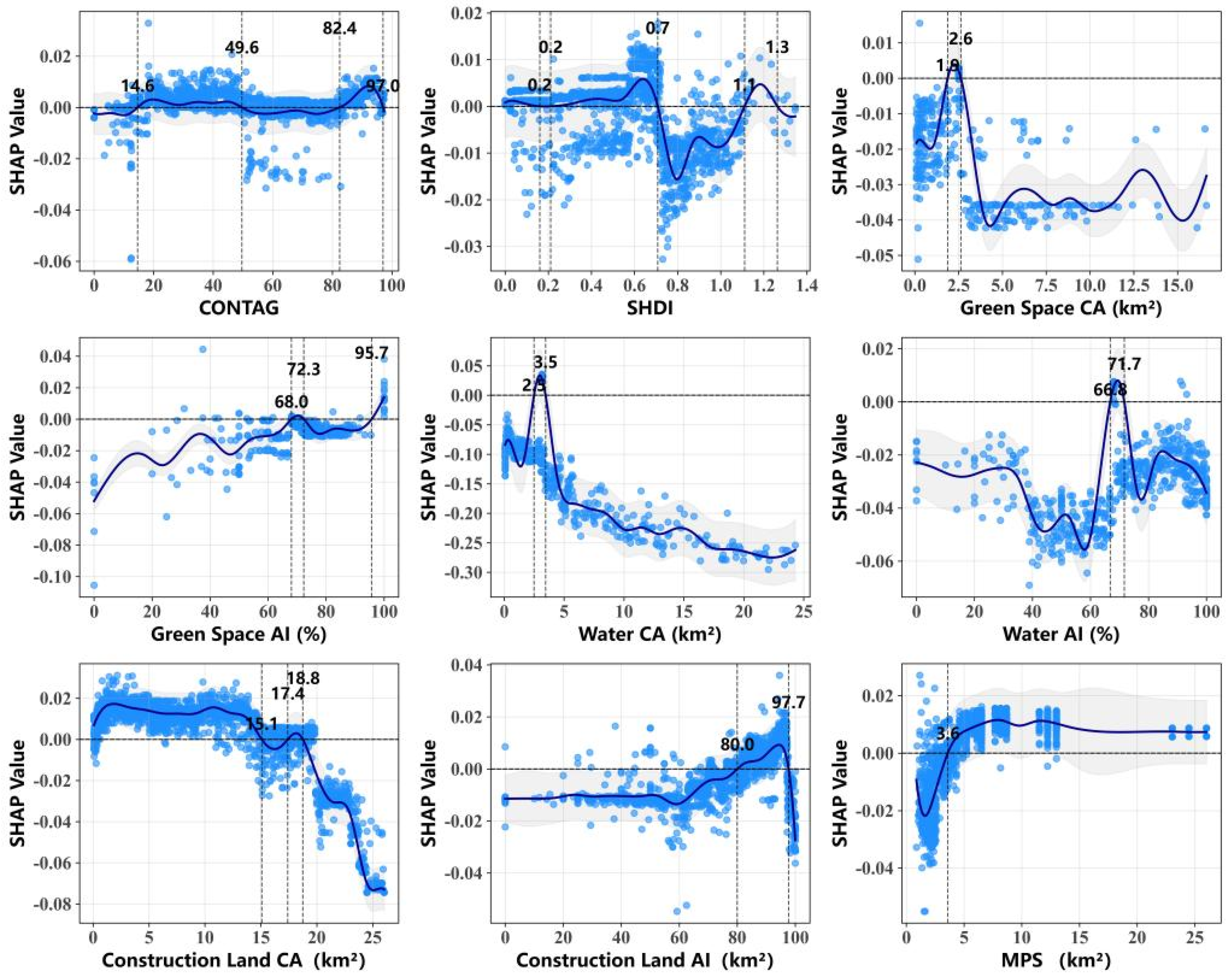
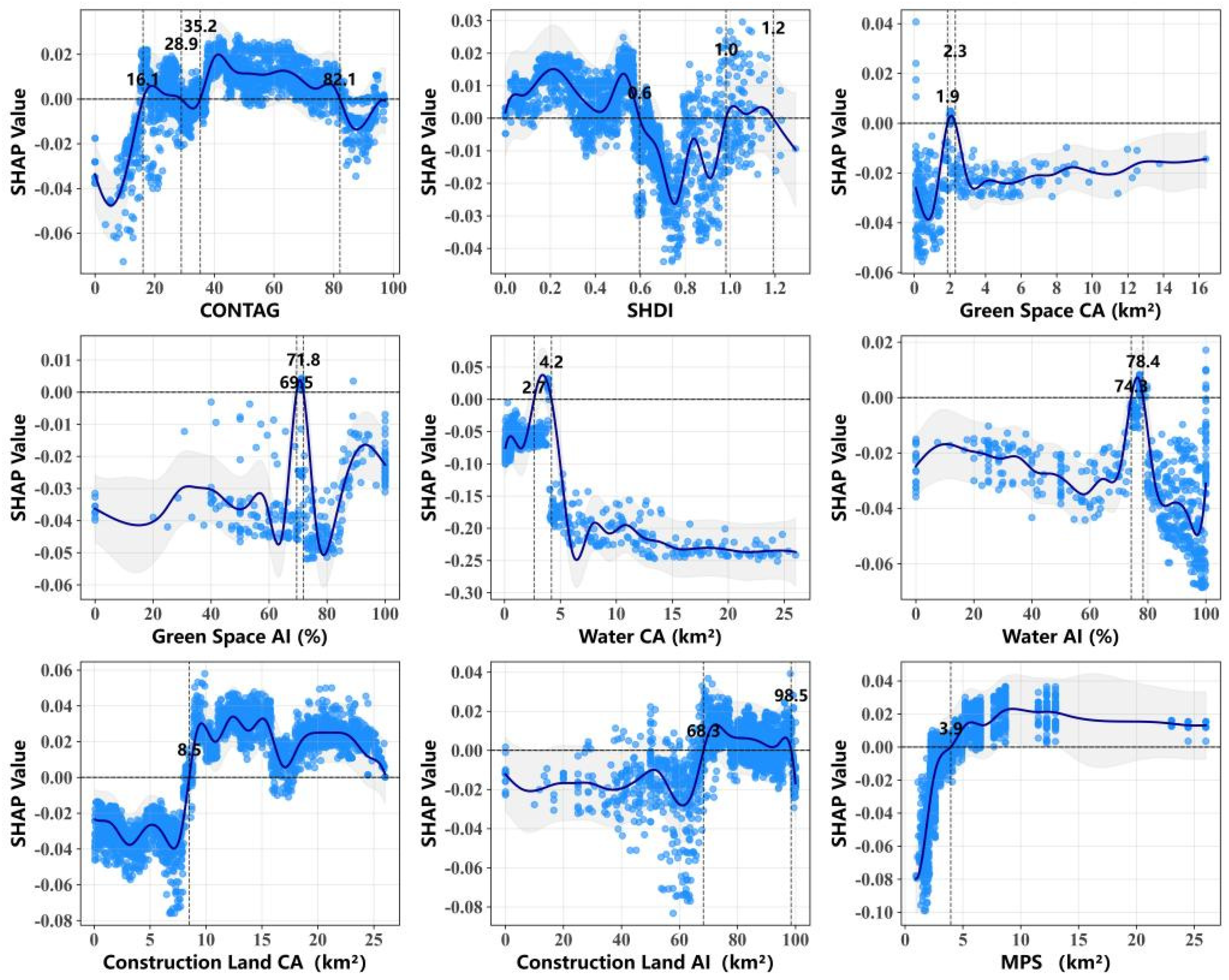
Based on inflection point identification in SHAP dependence plots combined with locally weighted scatterplot smoothing (LOESS) fitting (Figure 9 and Figure 10), this study accurately identifies the thresholds of core key factors (water body CA, built-up land CA) and effective thresholds of secondary factors (water body AI, built-up land AI, green space CA) for thermal environment regulation in Zhengzhou. This threshold system exhibits significant interannual differentiation and region-specific characteristics, reflecting the combined effects of thermal environment evolution and landscape structural changes under rapid urbanization in Zhengzhou, and provides quantitative boundaries for precise thermal environment regulation.

Threshold Response Characteristics of Key Landscape Factors

For 2015, the SHAP dependence plots revealed clear threshold effects. The cooling effect of the water body area intensified when the patch area exceeded approximately 3.5 km² (with an uncertainty range of 2.5–3.5 km² based on the zero-crossing interval). The warming threshold for built-up land area was identified at approximately 18.8 km² (range 17.4–18.8 km²); beyond this point, SHAP values increased sharply from about 0.1 to 0.4. When the green space aggregation index (green space AI) exceeded 72.3%, and the water body aggregation index (water body AI) exceeded 71.7%, their marginal effects shifted from warming to cooling. Pattern-related indicators such as CONTAG and SHDI exhibited bidirectional fluctuations, with the direction of their effects varying across value ranges.

For 2024, the thresholds were generally different, though with differentiated effect intensities. The effective cooling threshold for the water body area was higher, at approximately 4.2 km² (range 2.7–4.2 km²), and the cooling threshold for water body AI rose to 78.4%. The critical warming threshold for built-up land area was lower, at 8.5 km² (only negative SHAP values were observed beyond this point; no positive SHAP values were captured within the data range), and the warming effect further intensified when built-up land AI exceeded 68.3%. The cooling threshold for green space area slightly decreased from 2.6 km² (2015) to 2.3 km² (2024). In contrast, the bidirectional fluctuations of pattern-related indicators weakened, generally trending toward more stable marginal effects.

All thresholds are context-specific and exploratory: they are derived from Zhengzhou’s main urban area at 500 m grid resolution for the two studied years (2015, 2024) using the XGBoost model with default parameters. These indicative values should be interpreted with caution and used as reference ranges rather than fixed design standards, especially when applying to other cities or spatial scales. A comparison reveals that from 2015 to 2024, the regulatory thresholds of landscape composition and configuration on SUHII in Zhengzhou exhibited differentiated evolution: the cooling thresholds for water body size and aggregation significantly increased with urban expansion, indicating that maintaining the same cooling effect requires larger and better-connected blue–green spaces; meanwhile, the warming threshold for built-up land greatly decreased, implying that the sensitivity of the urban thermal environment to built-up land expansion has significantly increased, with even small-scale built-up land triggering strong warming effects. Overall, the dominant roles of the scale effects of water bodies and built-up land have become further accentuated, while the influence of pattern-related indicators has tended to stabilize, suggesting a possible pattern of “dominant scale effect and weakened configuration effect” under rapid urbanization, though continuous verification with multi-year data is needed.

6.3. Visualization Analysis of the Impact of Landscape Indicators on SUHII

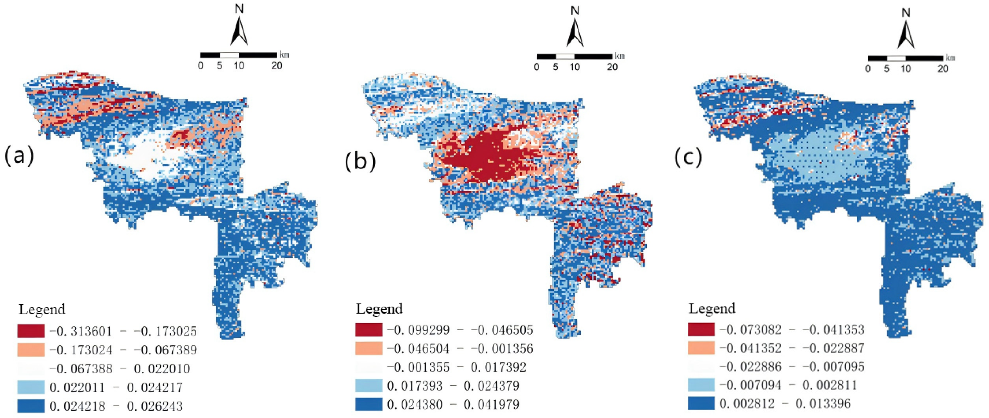
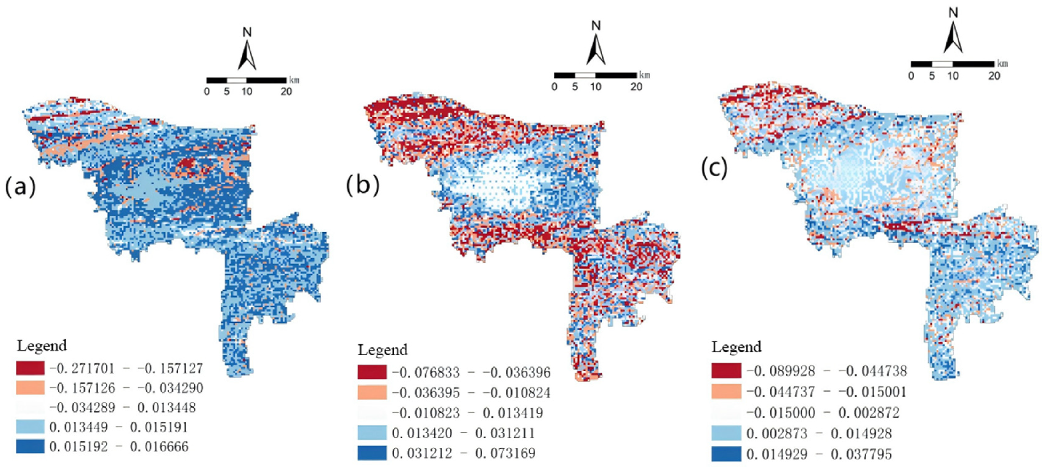
The pixel-scale spatial visualization of SHAP values overcomes the limitations of global statistical analysis and intuitively reveals the spatial differentiation characteristics of the marginal effects of various landscape composition and configuration indicators on surface urban SUHII. In this study, SHAP values were mapped onto the study area grid to produce spatial distribution maps of the marginal effects of core landscape indicators for 2015 and 2024. The results show that the cooling/warming marginal effects of landscape indicators exhibit significant spatial heterogeneity and are highly coupled with the spatial structure of Zhengzhou (Figure 11 and Figure 12).

6.3.1. Spatial Pattern of Marginal Effects in 2015

In 2015, the spatial distribution of SHAP values for each landscape indicator was consistent with the early urbanization pattern of Zhengzhou. Water CA: The SHAP values exhibited a cooling effect pattern of “strong in the northwest, weak in the southeast.” In the northwestern part of the central urban area, the SHAP values of water CA were significantly negative, indicating a prominent cooling marginal effect. In the southern part of the central urban area and the southeastern urban–rural transition zone, the SHAP values of water CA were close to zero or slightly positive, indicating that the cooling effect was masked. Construction Land CA: The SHAP values exhibited a “core–periphery” pattern of warming effect. In the central urban area, the SHAP values of Construction Land CA were significantly positive, indicating a strong warming marginal effect. In the peripheral new districts and urban–rural transition zones, the SHAP values of Construction Land CA were close to zero or slightly negative, suggesting that the warming effect could be mitigated. Water AI: The SHAP values exhibited a “localized patchy” cooling characteristic.

6.3.2. Spatial Pattern of Marginal Effects in 2024

In 2024, with the advancement of urban construction in Zhengzhou, the spatial pattern of marginal effects of landscape indicators evolved significantly. Water CA: The cooling marginal effect spread outward. In the peripheral new districts and urban–rural transition zones, the SHAP values of Water CA were significantly negative, indicating that the cooling effect radiated from the northwestern part of the central urban area to the periphery. In the southern part of the central urban area, the SHAP values of Water CA remained close to zero, suggesting that the issue of water fragmentation had not been resolved. Construction Land CA: The warming marginal effect expanded southward and eastward. In the peripheral new districts, the SHAP values of Construction Land CA were significantly positive, indicating an enhanced warming effect. In the central urban area, the SHAP values of Construction Land CA decreased slightly. The causes of this decrease are not directly identifiable from our dataset, and we refrain from attributing it to any specific policy or intervention without further evidence. While previous studies have suggested that urban greening or infrastructure measures may influence local thermal environments under certain conditions [48], confirming whether such factors contributed to the observed SHAP reduction would require dedicated local data and is beyond the scope of this study. MPS: The marginal effect exhibited a “mixed distribution” characteristic. In the urban–rural transition zones, the SHAP values of MPS were slightly positive, reflecting that the large average area of natural patches in this region had a certain regulating effect on the thermal environment, though the overall contribution was low.

Overall, the SUHII in Zhengzhou was higher in 2024 than in 2015, and the thermal environment shifted from localized high-temperature patches to a more continuous pattern of heat accumulation. The expansion of built-up land remains the primary driving factor for heat island intensification, while water bodies and green spaces exhibit a clear cooling effect. At the same time, the thermal environment sensitivity of the city to newly added built-up land is continuously increasing, whereas blue–green spaces need to reach a larger scale to achieve effective cooling.

7. Discussion

Based on Landsat 8 remote sensing images from 2015 to 2024, this study couples landscape pattern indices with the XGBoost-SHAP interpretable model to clarify the nonlinear driving mechanisms and regional threshold characteristics of landscape composition and configuration on urban SUHII in the urban area of Zhengzhou. The findings are consistent with global and regional urban thermal environment evolution patterns and can provide empirical support for precise heat island regulation in rapidly urbanizing inland cities.

7.1. General Patterns and Regional Characteristics of Urban Heat Island Differences Between 2015 and 2024

From 2015 to 2024, the SUHII in Zhengzhou was substantially higher, with its spatial pattern expanding from scattered patches to a continuous sheet, which is consistent with the patterns observed in other studies of urban heat island change over time (though our two-point comparison cannot itself confirm a trend). This is consistent with the scientific regularity that rapid urbanization is often accompanied by increasing SUHII and the coalescence of high-temperature areas, as reported in previous studies. However, we note that our two-point comparison does not itself constitute a direct test of this temporal regularity. As an inland plain city, Zhengzhou lacks the cooling effects of mountains and the regulation of sea–land breezes; thus, the expansion of its heat island is highly synchronized with the expansion of its built-up area, exhibiting an outward-expansion pattern of intensification [49]. This indicates that inland plain cities are more sensitive to land use change, and their thermal environment is easily dominated by built-up area expansion, showing distinct regional characteristics. This finding is highly consistent with the conclusions of spatiotemporal dynamic studies on surface heat islands in the Zhengzhou metropolitan area, and supports the view from global studies of large cities that rapid expansion of built-up land is the core factor driving the increase in SUHII, highlighting the uniqueness of thermal environment evolution in inland central cities [50].

7.2. Core Scientific Mechanisms of Landscape Composition and Configuration Driving the Urban Heat Island Effect

This study confirms that the landscape area effect is the primary driver of the change in the thermal environment, while the landscape composition and configuration effect is secondary, which is a common driving pattern in rapidly urbanizing areas. Green space area, water body area, and landscape diversity are negatively correlated with SUHII, while built-up land area and aggregation index are positively correlated. Pattern-related indicators such as mean patch area and contagion index play a weak role, indicating that the proportion of underlying surface type is the primary factor determining the surface thermal environment. As the urban thermal background intensifies, small-scale water bodies are unable to offset the warming effect of surrounding built-up land, requiring larger and more continuous blue spaces to achieve stable cooling. Water body CA had a mean SHAP value of 0.42 in 2015, compared to 0.21 for green space CA, indicating that water bodies provide approximately twice the cooling contribution per unit area, a pattern that is universal. This finding is consistent with the broader literature that landscape composition outweighs landscape configuration in explaining SUHII. Our results confirm that in Zhengzhou, land use structure is the dominant factor, while spatial configuration plays a secondary role.

7.3. Scientific Significance and Planning Value of Nonlinear Responses and Threshold Patterns

An important finding of this study is that landscape composition and configuration exhibit nonlinear responses to SUHII with clear effect thresholds, and that these thresholds differed between 2015 and 2024. Specifically, the effective cooling threshold for water bodies was higher in 2024 (4.2 km²) than in 2015 (3.5 km²), while the warming threshold for built-up land was lower (8.5 km² vs. 18.8 km²) and the warming threshold for built-up land decreased from 18.8 km² to 8.5 km². This comparison suggests that, between these two years, larger or better-connected blue–green spaces were associated with stable cooling, whereas the thermal environment becomes increasingly sensitive to even small-scale built-up expansion.

While the cooling and warming effects of land cover are well established, most previous studies have been static and have not provided planning-ready, time-specific thresholds. Our contribution is threefold: (1) a cross-stage threshold comparison between two time points (2015 and 2024); (2) reporting of empirical uncertainty ranges based on SHAP distributions; and (3) translation of thresholds into grid-specific planning benchmarks (e.g., water area ≥ 4.2 km² per 500 m grid; built-up patch size ≤ 8.5 km²). Thus, despite using standard methods, the application context—quantifying shifting thresholds and linking them to practice—extends existing knowledge, particularly for rapidly urbanizing cities. The pattern observed here may be applicable to other cities with similar characteristics, but local validation is required. We acknowledge that the thresholds reported here are derived from an exploratory, data-driven approach and lack formal statistical validation (e.g., confidence intervals). As such, they should be considered as indicative benchmarks that provide directional guidance for urban planning and thermal environment regulation, rather than prescriptive design standards. Urban planners and policymakers are encouraged to use these values in combination with local knowledge and to update them as more data become available.

7.4. Limitations

This study has several limitations. First, landscape pattern characterization was restricted to 2D metrics (patch area, AI, SHDI, CONTAG); 3D indicators (building height, floor area ratio) were not included due to data unavailability. However, since our SUHII is derived from satellite LST (surface, not canopy layer), the existing literature suggests that 2D composition remains the dominant control on LST even when vertical indicators are considered. Thus, while 3D omission may underestimate vertical configuration effects, it does not invalidate our core findings. Second, only two August images (2015 and 2024) were analyzed. This design intentionally controls seasonal and phenological variations, but two time points cannot capture continuous trends. Therefore, our findings should be interpreted as a snapshot comparison between two urbanization stages, not as a temporal trend. Accordingly, terms such as “increase,” “decrease,” “shift,” or “evolution” in this manuscript refer strictly to the observed differences between these two specific years and do not imply a continuous temporal trajectory. Statements about “higher/lower” refer strictly to the difference between these two years. Future dense time series are needed to confirm whether observed differences represent gradual evolution. Third, the XGBoost-SHAP framework is data-driven and does not encode physical laws. Our interpretations (e.g., latent heat flux for water bodies) are qualitative. Causality and process-based thresholds require integration with physical models (e.g., surface energy balance or LCZ). Fourth, meteorological variables (wind, humidity) and anthropogenic heat were omitted due to data availability. Their absence may affect estimated landscape-driven effects. Fifth, technical limitations: the XGBoost model used default parameters (though sensitivity analysis showed robustness, Appendix A Table A1); SHAP stability was not verified via bootstrapping; grid resolution (500 m) and daytime-only SUHII were not tested for sensitivity. Sixth, the thresholds identified via SHAP dependence plots are exploratory. We did not perform bootstrap or cross-validation to quantify sampling variability; the reported uncertainty ranges are descriptive measures of local SHAP dispersion, not formal confidence intervals. Seventh, while we have discussed several plausible mechanisms underlying the observed patterns (e.g., fragmentation of blue–green spaces, anthropogenic heat emissions, and potential infrastructure effects), these interpretations are speculative and are not directly supported by our dataset. We have therefore refrained from drawing strong causal conclusions from these mechanisms and explicitly noted where further dedicated data and analysis are needed. Consequently, these thresholds are best interpreted as indicative reference points for understanding nonlinear response patterns rather than as statistically validated cut-off values for policy implementation. Despite these limitations, the core findings—dominant roles of water bodies and built-up land, nonlinear responses, and threshold differences between the two years—remain robust within the defined scope (Zhengzhou main urban area, 500 m grid, August conditions of 2015 and 2024).

7.5. Planning Implications for Heat Island Mitigation in Zhengzhou

The threshold values identified in this study provide quantitative benchmarks for territorial spatial planning and blue–green space optimization in Zhengzhou.

7.5.1. Threshold-Based Design Recommendations

Water bodies: The cooling threshold was higher in 2024 (4.2 km²) than in 2015 (3.5 km²) at the 500 m grid scale. Water bodies or well-connected water networks should exceed 4.2 km² to achieve a stable cooling effect. Small, disconnected ponds (<1 km²) provide negligible cooling. Where large water bodies are infeasible, connecting smaller ones via ecological corridors can help approach the threshold.

Built-up land: The warming threshold for contiguous built-up area decreased from 18.8 km² (2015) to 8.5 km² (2024). We recommend that new development patches should not exceed 8.5 km² of contiguous built-up area at the 500 m grid scale. Larger developments should be interleaved with blue–green corridors to prevent any single patch from crossing the threshold.

Green spaces: Green space area plays a secondary role compared to water bodies, with a cooling threshold of 2.3–2.6 km². Green spaces below this size have limited cooling effects and should be designed as connected networks rather than isolated patches.

Aggregation indices: Built-up land aggregation index (AI) exceeding 68.3% significantly exacerbates SUHII. Compact, block-scale developments without internal blue–green breaks should be avoided. For water bodies, AI increased from 71.7% (2015) to 78.4% (2024), indicating that highly connected water networks produce stronger cooling.

7.5.2. Pathways for Planning Implementation

We propose three pathways to translate these thresholds into practice:

(1) Grid-based zoning: Grids where water body area < 4.2 km² can be designated as “cooling priority zones” for blue-space restoration. Grids where built-up patch size is >8.5 km² or AI > 68.3% can be designated as “heat risk mitigation zones” requiring green infrastructure retrofits.

(2) Urban renewal guidelines: In highly built-up areas where large water bodies cannot be created, the built-up AI threshold (68.3%) can identify “heat-prone blocks” where green roofs, permeable pavement, and pocket parks should be prioritized.

(3) Adaptive monitoring system: As Zhengzhou continues to urbanize, thresholds will shift. We recommend updating these thresholds every 3–5 years using satellite data to maintain adaptive, evidence-based planning.

7.5.3. From Qualitative Principles to Quantifiable Indicators

These thresholds move beyond general recommendations (e.g., “increase blue–green space”) toward spatially explicit, quantifiable control indicators that can be mapped and monitored. For example, a planner can overlay a 500 m grid on a proposed development zone, calculate existing water body area per grid, and check whether it meets the 4.2 km² threshold. The methodological framework is transferable to other rapidly urbanizing regions, though thresholds should be locally calibrated.

7.6. Generalizability and Applicability Conditions

Our findings are most directly applicable to cities with (1) a temperate monsoon climate (hot summers); (2) flat, plain topography; (3) rapid, outward-expanding, high-density urbanization; and (4) large or megacity scale (>3 million). These conditions match Zhengzhou’s setting. Transferability to tropical, arid, or cold climates, mountainous or coastal terrains, or low-density sprawling urban forms requires additional validation. The threshold values (e.g., water body cooling threshold of 3.5–4.2 km²) should be used as reference ranges rather than universal constants, and local calibration is recommended.

8. Conclusions

Based on land surface temperature retrieved from Landsat 8 remote sensing images in 2015 and 2024, combined with landscape pattern indices, Pearson correlation analysis, and the XGBoost-SHAP interpretable model, this study systematically analyzes the driving mechanisms and nonlinear response characteristics of urban landscape composition and configuration on SUHII. Taking Zhengzhou as a case study, several common patterns of urban thermal environment evolution and landscape regulation in rapidly urbanizing areas are identified:

1. Between 2015 and 2024, the heat island in Zhengzhou showed a pattern of intensification and spatial expansion: the average SUHII was higher in 2024, and the area of strong/extreme heat islands was substantially larger.

Consistent with the observed differences between 2015 and 2024, the urban thermal environment in Zhengzhou showed a transition from a pattern of “scattered high-temperature patches” to a more “continuous high-temperature area” as built-up land expanded. In Zhengzhou, the average SUHII was higher in 2024 (11.51 °C) than in 2015 (6.22 °C), and the area proportions of strong and extremely strong heat islands were substantially larger in 2024, indicating a clear structural intensification trend of the urban heat island during the rapid urbanization phase. This observed difference reflects the effect of built-up land expansion and impervious surface increase on the urban thermal environment.

2. The compositional structure of the landscape has a stronger influence on the urban thermal environment than the spatial configuration of the landscape, representing the key mechanism of urban heat island formation.

The results show that landscape area-based indicators have significantly higher explanatory power for SUHII than landscape pattern-based indicators. Water body area and green space area are significantly negatively correlated with SUHII, while built-up land area and its aggregation index are significantly positively correlated. In contrast, pattern-related indicators such as mean patch area and contagion index play relatively weaker roles. This finding indicates that during rapid urbanization, land use structural change is the dominant factor determining the urban thermal environment, whereas landscape spatial configuration mainly plays a supplementary regulatory role.

3. Blue–green spaces have a significant cooling effect, with water bodies generally contributing more to thermal environment regulation than green spaces.

SHAP feature importance analysis shows that water body patch area is the primary cooling factor affecting SUHII, while built-up land area is the most important warming factor. Water bodies generate a stable cooling effect through processes such as evaporative cooling, high heat capacity, and heat exchange, and their cooling intensity is significantly higher than that of vegetation transpiration from green spaces. This result indicates that in urban thermal environment regulation, the construction of large, continuous water bodies and blue–green space networks is an important means of mitigating the urban heat island.

4. Landscape composition and configuration exhibit significant nonlinear responses and threshold effects on the urban thermal environment.

A key contribution of this study is the quantification of how regulatory thresholds differed between two urbanization stages (2015 and 2024). While previous studies have recognized the cooling effect of water bodies and the warming effect of built-up land, most have treated thresholds as static. Our comparison of 2015 and 2024 shows that: the water body cooling threshold was higher in 2024 (4.2 km²) than in 2015 (3.5 km²); the built-up warming threshold was lower (8.5 km² vs. 18.8 km²), indicating a much higher thermal sensitivity to contiguous development in the later stage.

These cross-stage differences provide quantitative targets for blue–green space planning and built-up land control in Zhengzhou. The empirical uncertainty ranges (provided in Appendix B) further inform planners of the inherent variability around these thresholds. When the water body area exceeds a certain scale, its cooling effect significantly intensifies; whereas when the built-up land area exceeds a critical value, it markedly exacerbates the heat island effect. The case study of Zhengzhou shows that the effective cooling threshold for water bodies was higher in 2024 (4.2 km²) than in 2015 (3.5 km²), while the warming threshold for built-up land was lower in 2024 (8.5 km²) than in 2015 (18.8 km²), suggesting that between these two years, the sensitivity of the thermal environment to built-up land expansion was higher in the later stage. However, confirmation of a continuous increase would require additional multi-year data. This pattern indicates that urban thermal environment regulation depends not only on landscape type but also on its scale and spatial thresholds.

In summary, the formation and evolution of the urban heat island effect are primarily driven by the combined effects of built-up land expansion and changes in blue–green spaces. In the context of rapid urbanization, relying solely on scattered green spaces is insufficient to effectively mitigate the thermal environment. Greater attention should be paid to the large-scale protection and systematic configuration of blue–green spaces. By controlling the scale of contiguous built-up land, constructing large-scale blue–green ecological networks, and optimizing urban spatial structure, long-term stable regulation of the urban thermal environment can be achieved. These findings are derived specifically from Zhengzhou’s main urban area (2015–2024) at 500 m grid resolution. Broader generalization requires further testing in other cities and under different climatic and spatial conditions. Given that only two time points were analyzed, these conclusions refer to differences observed between 2015 and 2024 and should not be overinterpreted as evidence of a continuous temporal trend without further multi-year data. Within this scoped contribution, we believe the observed cross-stage differences provide useful reference points for both local planning and the design of future multi-year monitoring efforts.