Spatial Coupling of Vegetation Frontline Migration and Vegetation-Cover Change on the Eastern Bank of the Liaohe Estuary Based on Multi-Source Remote Sensing (2000–2025)

Abstract

This study investigated vegetation frontline dynamics, fractional vegetation cover (FVC), and community succession in the tidal-flat wetlands of the Liaohe Estuary. The eastern bank of the Liaohe River within the Shuangtaihe National Nature Reserve was selected as the study area, and six periods of Landsat and Gaofen-1 (GF-1) imagery from 2000 to 2025 were used. Remote-sensing preprocessing, normalized difference vegetation index (NDVI)-based FVC inversion, vegetation frontline extraction, Digital Shoreline Analysis System (DSAS)-based rate calculation, land-cover classification, and spatial correlation analysis were integrated to characterize wetland spatiotemporal dynamics and succession patterns. The results showed that the linear regression rate (LRR) and end point rate (EPR) effectively captured the long-term trend and five short-term fluctuations in vegetation frontline migration. FVC fluctuated markedly over the 25-year period, whereas the weighted average (WA) of the five FVC classes remained generally stable and effectively summarized overall vegetation growth. Vegetation frontline migration was spatially associated with annual FVC change (ΔFVC); both LRR and ΔFVC showed significant positive spatial autocorrelation and evident spatial clustering. In addition, the conversion among mudflats, Suaeda salsa, Phragmites australis, and water bodies was closely coupled with frontline migration. These findings provide a scientific basis for quantifying coastal wetland sustainability and for designing spatially targeted restoration strategies in the Liaohe Estuary. The proposed coupling analysis framework also offers a transferable remote sensing approach for monitoring wetland sustainability under changing environmental conditions.

1. Introduction

Coastal tidal-flat wetlands are ecological transition zones shaped by land–sea interactions. The advance and retreat of vegetation frontlines, together with changes in fractional vegetation cover (FVC), directly reflect wetland succession and ecosystem condition [1,2]. Located in Northeast China, the Shuangtaihe National Nature Reserve of the Liaohe Estuary is a representative tidal-flat wetland dominated by Phragmites australis and Suaeda salsa [3]. This wetland provides important ecological functions, including biodiversity maintenance, carbon sequestration, and coastal protection [4]. In recent decades, reduced riverine sediment discharge, sea-level rise, land reclamation, aquaculture activities, and other natural and anthropogenic disturbances have reshaped vegetation boundaries in this region [1,5,6]. These disturbances have also produced complex spatial differentiation in FVC and have promoted degradation or succession of native halophytic vegetation. Therefore, a systematic analysis of the coupling among vegetation frontline migration, vegetation-cover change, and community succession is essential for wetland conservation and restoration.

Remote sensing provides long-term, spatially continuous, and repeatedly observed data and has therefore become a principal tool for monitoring coastal wetlands [7,8]. The Digital Shoreline Analysis System (DSAS) can quantify vegetation frontline movement by calculating the linear regression rate (LRR) for long-term change and the end point rate (EPR) for short-term change from multi-temporal frontline positions [9,10,11,12]. In parallel, FVC retrieval based on the pixel dichotomy model and least-squares trend fitting can characterize vegetation-cover dynamics. Spatial autocorrelation analysis, including Global and Local Moran’s I, further reveals whether vegetation variables are spatially clustered or randomly distributed [13]. Finally, by overlaying transect data with vegetation-type maps, the frequency and direction of land-cover conversion can be used to interpret community succession.

Although many studies have examined shoreline migration or FVC change separately, quantitative evidence for the spatial coupling between vegetation frontline dynamics (LRR and EPR) and the annual change rate of FVC (ΔFVC) remains limited. In addition, the relationship between short-term vegetation-type conversion and short-term vegetation frontline migration has rarely been evaluated at the transect scale.

Recent work in salt-marsh ecogeomorphology has emphasized the two-way feedback between vegetation dynamics and sediment processes [14]. Vegetation frontline migration can be both a driver and a consequence of sedimentation [15], and the resulting elevation changes regulate species zonation through habitat filtering [16]. Salt-marsh vegetation also affects sediment transport and deposition [17]. In the Liaohe Delta, field measurements indicate that Phragmites australis marshes have higher rates of surface-elevation change and vertical accretion than Suaeda salsa marshes [18]. Climate change and human activities have further altered the distribution and cover of these two species over recent decades [19,20], while vegetation can reduce wave erosion along salt-marsh edges [21]. However, few studies have explicitly linked frontal migration rates with FVC trends at the transect scale. The spatial relationship between frontline advance or retreat and FVC change therefore remains insufficiently quantified. To address this gap, this study integrates long-term remote sensing, DSAS analysis, FVC trend estimation, and spatial autocorrelation to examine biogeomorphic feedback in the Liaohe Estuary.

To address these gaps, this study uses the eastern bank of the Liaohe Estuary as the study area and analyzes six periods of remote-sensing imagery from 2000 to 2025. The specific objectives are to: (1) extract vegetation frontlines and calculate LRR and EPR; (2) estimate FVC using the pixel dichotomy model, classify FVC into five grades, calculate the weighted average (WA) of the five FVC classes [22], and derive ΔFVC through least-squares fitting; (3) extract ΔFVC values at transect points and evaluate their relationship with LRR using correlation and four-category statistics; (4) analyze the spatial autocorrelation of LRR and ΔFVC using Global and Local Moran’s I; and (5) visualize vegetation-type conversion patterns for EPR intervals using chord diagrams. Through these analyses, this study aims to clarify the spatial coupling among vegetation frontline advance or retreat, vegetation-cover change, and community succession, thereby providing a scientific basis for estuarine wetland protection and restoration.

Compared with studies that analyze shoreline change and vegetation cover separately, this study quantifies their coupling at the transect scale. Understanding this coupling is important for testing salt-marsh biogeomorphic feedback, such as whether frontal advance is accompanied by FVC increase, and for improving wetland restoration planning under changing sediment supply and sea-level conditions.

The normalized difference vegetation index (NDVI) was selected instead of the kernel normalized difference vegetation index (KNDVI) and sun-induced chlorophyll fluorescence (SIF) because it is better suited to the long-term intertidal wetland analysis conducted here. NDVI is a classical vegetation index based on red and near-infrared reflectance, has stable performance, and is supported by complete long-term image records. These characteristics make it suitable for FVC retrieval in mixed landscapes composed of mudflats and halophytic vegetation. By contrast, KNDVI is optimized primarily for dense forests and high-biomass vegetation, and its advantage in reducing saturation is less relevant to moderately or sparsely distributed salt-marsh plants. SIF mainly reflects photosynthetic activity and stress status and requires specialized hyperspectral sensors. Continuous SIF datasets are not available for the 2000–2025 study period, which limits its applicability for long-term monitoring in this region. Previous regional studies of the Liaohe Estuary have also shown that NDVI performs well in retrieving the coverage of Suaeda salsa and Phragmites australis.

By quantifying the spatial coupling between vegetation frontline migration and vegetation-cover change, this study contributes to the broader goal of measuring and monitoring coastal wetland sustainability. The methodological framework developed here can serve as a sustainability assessment tool for estuarine wetlands affected by sea-level rise, reduced sediment supply, and intensified human disturbance.

2. Materials and Methods

2.1. Study Area

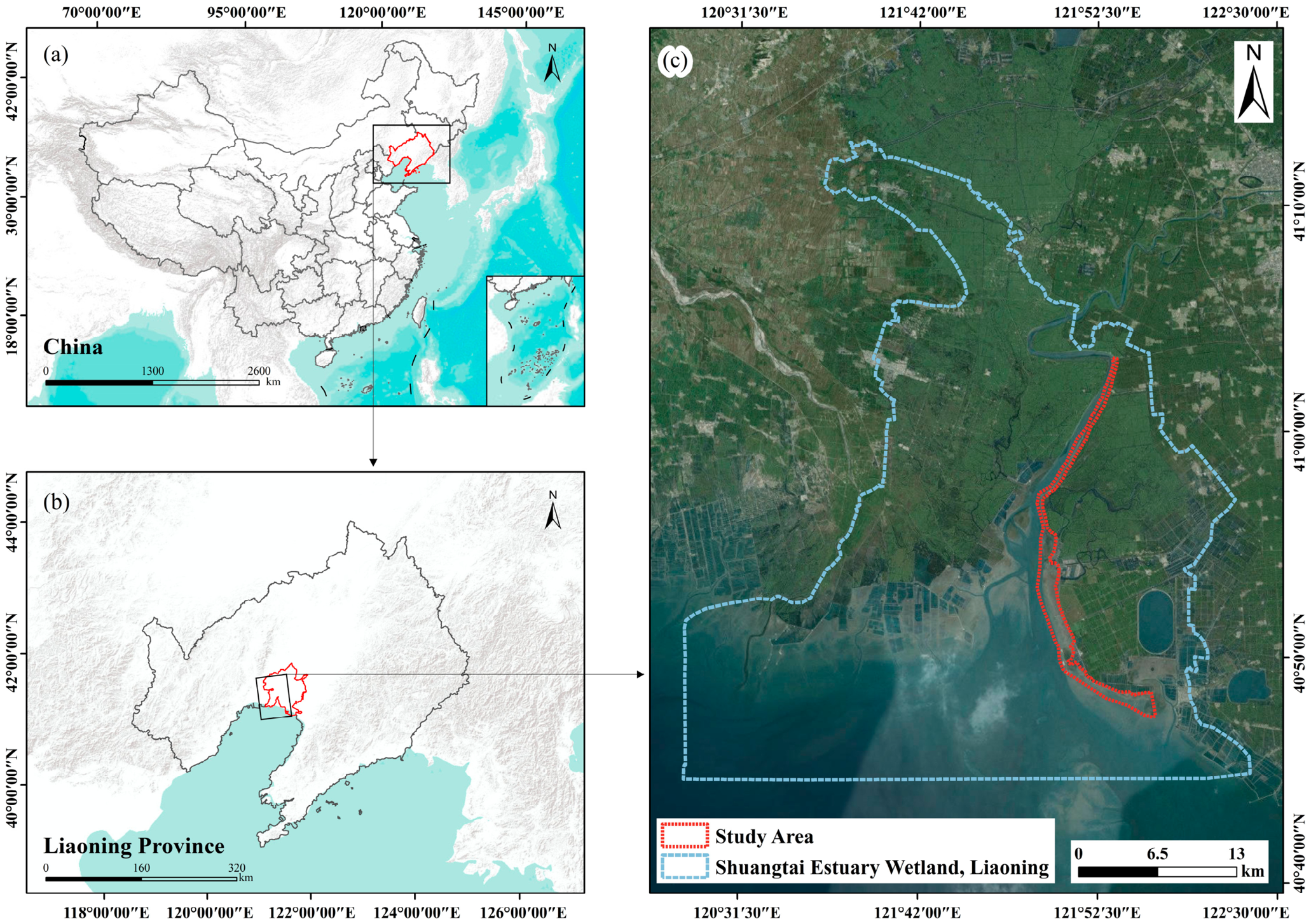
The study area is the eastern-bank tidal-flat wetland of the Shuangtaihe National Nature Reserve in the Liaohe Estuary (Figure 1), located between 40°45′–41°05′ N and 121°30′–122°00′ E [23,24]. The terrain is low and flat, with elevations of approximately 0.5–3 m. Under the combined influence of river discharge, sediment supply, tidal dynamics, and human activities, both the shoreline and vegetation boundary are highly dynamic. The region has a warm temperate semi-humid monsoon climate, with an annual mean temperature of approximately 8.5 °C and annual precipitation of about 650 mm, most of which occurs from June to September. The native vegetation is dominated by Suaeda salsa and Phragmites australis [25,26,27], forming the well-known “Red Beach” landscape. The eastern side of the study area is adjacent to the main tidal channel of the Liaohe River, whereas the western side is bounded by aquaculture ponds. Over the past two decades, reduced water and sediment discharge, port construction, and aquaculture reclamation have caused pronounced advance-retreat fluctuations in the vegetation frontline, while FVC has shown marked spatiotemporal differentiation [28]. Therefore, this area is well suited for studying vegetation dynamics in estuarine wetlands [25].

2.2. Remote-Sensing Data Sources and Preprocessing

The remote-sensing images used in this study consisted of Landsat 5 Thematic Mapper (TM) images acquired in 2000 and 2005, Landsat 7 Enhanced Thematic Mapper Plus (ETM+) images acquired in 2010, and Gaofen-1 (GF-1) Wide Field View (WFV) images acquired in 2015, 2020, and 2025. Specifically, the GF-1 datasets included WFV3 imagery for 2015, WFV2 imagery for 2020, and WFV1 imagery for 2025. All images were radiometrically calibrated and atmospherically corrected using the Fast Line-of-sight Atmospheric Analysis of Spectral Hypercubes (FLAASH) model in ENVI 5.6 (Harris Geospatial Solutions, Broomfield, CO, USA) and were uniformly projected to the World Geodetic System 1984 Universal Transverse Mercator Zone 51N (WGS 1984 UTM Zone 51N) coordinate system. Fine geometric registration was then performed, and registration errors were controlled within 0.5 pixels. In total, nine high-quality images with cloud cover of no more than 1% were used for vegetation frontline extraction and subsequent analyses. The study monitored approximately 40 km of tidal-flat wetland, and transects were generated at a spacing of 500 m. Because the resolution difference between 16 m and 30 m is substantially smaller than the analysis scale, its influence on the monitoring results is considered negligible. Therefore, subsequent analyses were performed at the original image resolutions. Detailed information for each image is provided in

Table 1. Satellite data information.

Date	Satellites and Sensors	Spatial Resolution (m)	Total Number of Scenes	Cloud Cover (%)
8 September 2000	Landsat 5 TM	30	2	0
6 September 2005	Landsat 5 TM	30	2	0
28 September 2010	Landsat 7 ETM+	30	2	0
21 September 2015	GF-1 WFV3	16	1	0
26 September 2020	GF-1 WFV2	16	1	0
20 September 2025	GF-1 WFV1	16	1	1

The images from 2000, 2005, and 2010 were each mosaicked from two adjacent scenes (path/row 120/031 and 120/032), whereas the images from 2015, 2020, and 2025 were single scenes.

.

All Landsat and GF-1 images were acquired in September of the corresponding survey year. July and August were avoided because frequent rainfall and fluctuating water levels can interfere with land-cover classification, whereas both Suaeda salsa and Phragmites australis generally maintain stable and mature growth conditions in September. Potential phenological bias caused by the early-to-late September acquisition difference was minimized by selecting cloud-free images (cloud cover of no more than 1%) that satisfied consistent geometric and atmospheric correction standards. The acquisition dates in Table 1 therefore represent the most feasible image combination for maintaining the 5-year sampling interval while ensuring image quality. Unlike the high-water line, the vegetation line is relatively stable because short-term tidal fluctuations and seasonal variability have limited effects on its position, and the clear reflectance contrast between vegetation and non-vegetation facilitates identification in medium-resolution imagery [10]. Unmanned aerial vehicle (UAV) photographs acquired on 26 September 2025 in representative areas (Figure S1) provide additional field evidence for identifying the vegetation–mudflat boundary. Moreover, the Otsu thresholds were consistently stable across years (0.20–0.25;

Table 2. Optimal Otsu thresholds for NDVI segmentation in each period.

Year	Otsu Threshold
2000	0.20
2005	0.25
2010	0.20
2015	0.20
2020	0.20
2025	0.25

), confirming robust spectral separability between vegetated and non-vegetated surfaces. Thus, the absence of explicit tidal records does not compromise the reliability of the extracted vegetation frontlines. To ensure temporal comparability, all remote-sensing datasets were processed using identical procedures, including Otsu threshold segmentation, five-level FVC classification, and multi-temporal least-squares fitting.

2.3. Research Methods

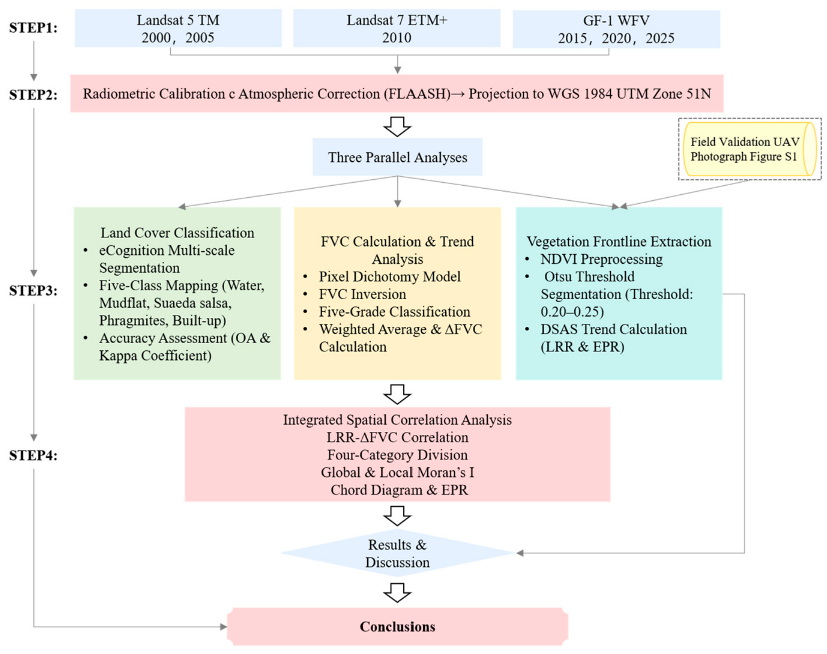
The methodological framework of this study is shown in Figure 2. The workflow consists of three stages: remote-sensing data acquisition and preprocessing; three parallel analyses, including vegetation frontline extraction, FVC estimation, and land-cover classification; and integrated spatial analysis and interpretation.

2.3.1. Vegetation Frontline Extraction and DSAS Analysis

NDVI was calculated for each of the six image periods using the band-math tool in ENVI 5.6 [29]. The formula is as follows:

$$NDVI={\displaystyle \frac{NIR-R}{NIR+R}}$$

(1)

where NIR is the near-infrared band reflectance, and R is the red band reflectance.

The Otsu algorithm, also known as the maximum inter-class variance method, was used to automatically determine the optimal segmentation threshold between vegetation and non-vegetation in each NDVI image [30]. This algorithm selects the threshold that maximizes the inter-class variance between the two pixel classes. The inter-class variance is calculated as follows:

$${\sigma }_B^2\left(k\right)={\omega }_0{\left({\mu }_0-{\mu }_T\right)}^2+{\omega }_1{\left({\mu }_1-{\mu }_T\right)}^2$$

(2)

where k is the gray-level threshold; ${\sigma }_B^2\left(k\right)$ is the between-class variance at threshold k; ${\omega }_0$ and ${\omega }_1$ are the probabilities of the background class and the target vegetation class, respectively; ${\mu }_0$ and ${\mu }_1$ are the mean gray values of the background and target vegetation classes, respectively; and ${\mu }_T$ is the mean gray value of the entire image. The optimal threshold is determined by the value of k that maximizes ${\sigma }_B^2\left(k\right)$. The optimal thresholds for each period are shown in Table 2. The thresholds ranged from 0.20 to 0.25, effectively separating halophytic vegetation (Suaeda salsa and Phragmites australis) from non-vegetated surfaces such as mudflats and water bodies.

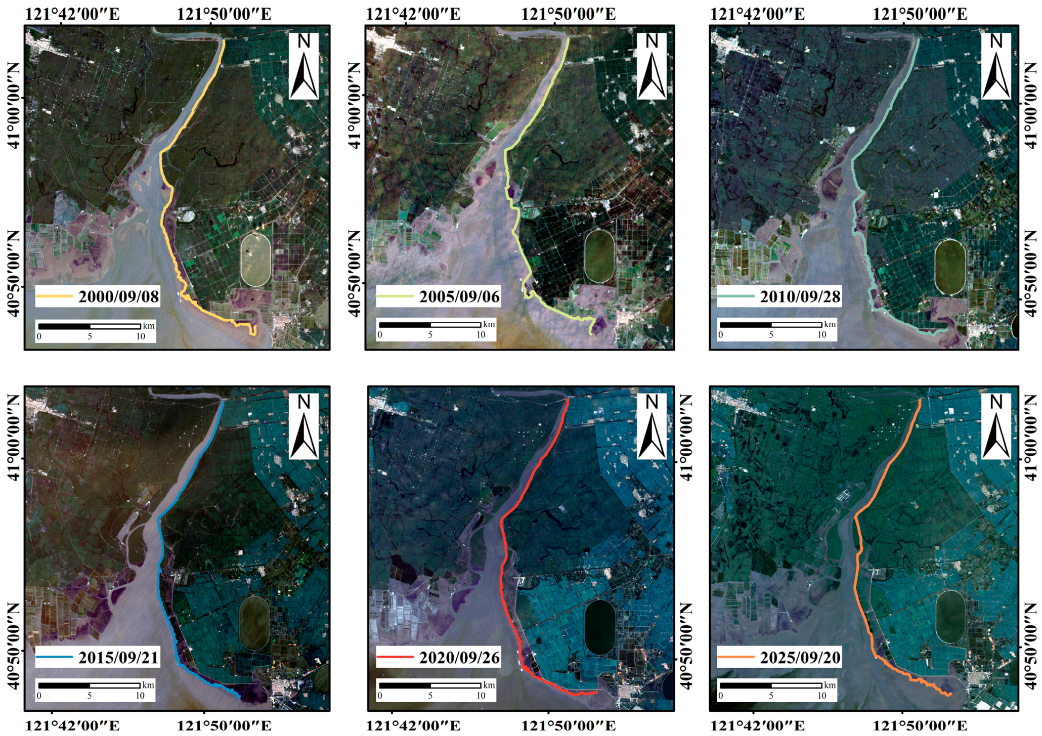
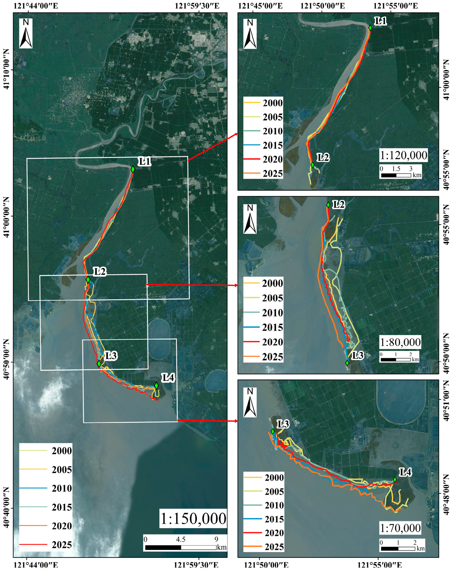
Pixels with NDVI values greater than or equal to the threshold were classified as vegetation, whereas pixels with NDVI values lower than the threshold were classified as non-vegetation. A binary vegetation-distribution map was generated for each period. Vegetation-patch boundaries were then obtained through raster-to-vector conversion, followed by manual visual correction to remove isolated patches smaller than 100 m² and jagged boundaries caused by tidal creeks. The final vegetation frontlines for each year are shown in Figure 3.

Based on the extracted vegetation frontlines, the DSAS v5.1 (U.S. Geological Survey, Woods Hole, MA, USA) extension in ArcGIS 10.8 (Esri, Redlands, CA, USA) was used to generate transects perpendicular to the shoreline. The vegetation frontline along the eastern bank of the study area was approximately 40 km long, and transects were generated at a uniform spacing of 500 m [12]. Because the vegetation frontline advanced or retreated among different years, the number of valid transects used in rate calculation varied slightly among periods; however, the transect layout maintained the same 500 m spacing throughout the analysis.

LRR was used to quantify long-term vegetation frontline change. For each transect, a simple linear regression was fitted between year x (x = 1, …, 6) and vegetation frontline position y. The slope of the regression represents LRR, with units of m/yr. The regression equation is as follows:

$$\begin{gathered} y=a+bx \\ a=\sum _{i=1}^n\left(x_i-\overline{x}\right)\left(y_i-\overline{y}\right) \\ b=\overline{y}-a\overline{x} LRR = b \end{gathered}$$

(3)

EPR was used to quantify short-term vegetation frontline change and was calculated from the two end point positions within each time interval:

$$EPR={\displaystyle \frac{y_2-y_1}{t_2-t_1}}$$

(4)

where y₁ and y₂ are the vegetation frontline positions at the beginning and end of a given period, respectively, and t₁ and t₂ are the corresponding years. Five intervals were analyzed: 2000–2005, 2005–2010, 2010–2015, 2015–2020, and 2020–2025.

2.3.2. Fractional Vegetation Cover (FVC) Calculation and Trend Analysis

(1) FVC calculation and classification

An improved pixel dichotomy model was used to estimate FVC in the study area [31]. The model constructs an empirical relationship based on NDVI and improves the accuracy of vegetation-cover estimation in coastal wetlands with either high or low vegetation cover. Therefore, it is suitable for monitoring halophytic vegetation dynamics on tidal flats. The formula is as follows:

$$\mathit{FVC}={\displaystyle \frac{\mathit{NDVI}-{\mathit{NDVI}}_{\mathit{soil}}}{{\mathit{NDVI}}_{\mathit{veg}}-{\mathit{NDVI}}_{\mathit{soil}}}}$$

(5)

where ${\mathrm{NDVI}}_{\mathrm{soil}}$ and ${\mathrm{NDVI}}_{\mathrm{veg}}$ are the NDVI values of bare soil and pure vegetation, respectively, taken as the 5% and 95% percentiles of the cumulative frequency [32]. Based on the vegetation characteristics of the tidal-flat wetland in the Liaohe Estuary, FVC was classified into five levels (

Table 3. FVC classification standard for the Liaohe Estuary coastal wetland.

FVC Grades	FVC Range	Surface Landscape Type
Extremely Low (EL)	0 ≤ FVC < 0.2	Bare mudflats, water bodies, unvegetated mudflats
Low (L)	0.2 ≤ FVC < 0.4	Sparse Suaeda salsa, low-coverage tidal-flat vegetation
Medium (M)	0.4 ≤ FVC < 0.6	Moderately covered Suaeda salsa community, low-density Phragmites australis
High (H)	0.6 ≤ FVC < 0.8	Highly covered Suaeda salsa, medium-density Phragmites australis community
Extremely High (EH)	0.8 ≤ FVC ≤ 1.0	High-density Phragmites australis

).

In this study, the weighted average (WA) of the five FVC classes was calculated to summarize the overall vegetation-cover status of the study area. The area percentage of each FVC class was used as the weighting factor, and the five FVC classes were assigned scores from 0 to 4, corresponding to extremely low, low, medium, high, and extremely high vegetation cover, respectively. WA was calculated as follows:

$$WA={\displaystyle \frac{EL\times 0+L\times 1+M\times 2+H\times 3+EH\times 4}{100}}$$

(6)

Remark 1.

EL, L, M, H, and EH represent the area percentages of the extremely low-, low-, medium-, high-, and extremely high-FVC classes, respectively, and their values range from 0 to 100%. WA ranges from 0 to 4, with higher values indicating a greater proportion of high-cover vegetation.

(2) Annual change rate of FVC (ΔFVC)

For each pixel, a least-squares linear regression was fitted using the year index t = 1, 2, 3, 4, 5, and 6 (corresponding to 2000, 2005, …, 2025) as the independent variable and FVC as the dependent variable:

$$FVC = a + b \cdot t$$

(7)

The slope b was calculated as follows:

$$b={\displaystyle \frac{6\sum \left(t\cdot FVC\right)-\sum t\sum FVC}{6\sum t^2-{\left(\sum t\right)}^2}}$$

(8)

Because each step in t represents 5 years, ΔFVC was calculated as follows:

$$\Delta FVC={\displaystyle \frac{b}{5}}$$

(9)

2.3.3. Vegetation Classification and Conversion Analysis

Land cover in the six image periods was classified in eCognition Developer 9 (Trimble Germany GmbH, Munich, Germany) using a method that combined multi-scale segmentation and threshold segmentation. Five classes were identified: water body, mudflat, Suaeda salsa, Phragmites australis, and built-up land. To assess classification accuracy, 180 random validation points with a minimum spacing of 50 m were generated for each period. Actual land-cover types were determined by visual interpretation of high-resolution imagery. The classification results were then extracted using the “Extract Values to Points” tool in ArcGIS 10.8, and a confusion matrix was constructed. Overall accuracy (OA) and the Kappa coefficient [33] were calculated as follows:

$$\mathrm{OA}={\displaystyle \frac{{\sum }_{i=1}^n{x}_{ii}}{N}}$$

(10)

$$\mathit{Kappa}={\displaystyle \frac{N{\sum }_{i=1}^n{x}_{ii}-{\sum }_{i=1}^n\left(x_{i+}\times x_{+i}\right)}{N^2-{\sum }_{i=1}^n\left(x_{i+}\times x_{+i}\right)}}$$

(11)

where $x_{ii}$ is the number of correctly classified samples for class i, N is the total number of samples, $x_{i+}$ is the number of actual samples for class i, $x_{+i}$ is the number of predicted samples for class i, and n is the number of classes (n = 5).

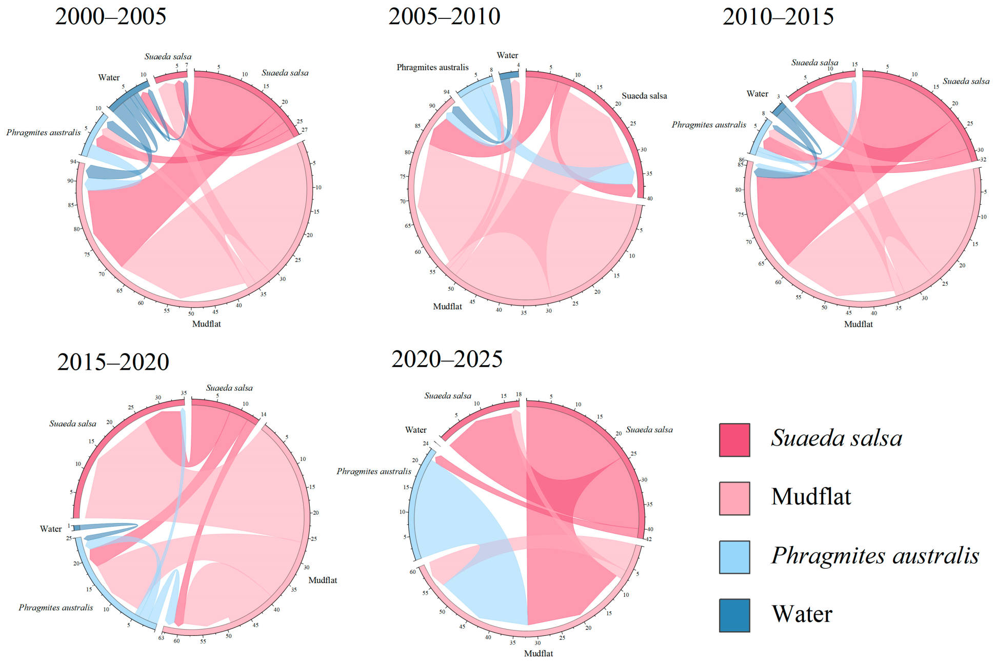
The classified land-cover maps were further overlaid with the intersections between vegetation frontlines and transects for each period. The vegetation type at each transect intersection was extracted for the start and end years of each interval. Conversion frequencies, expressed as the number of transects following each “start type → end type” pathway, were then calculated. Chord diagrams were used to visualize the dynamic conversion patterns along the vegetation frontline.

2.3.4. Correlation Analysis Between LRR and ΔFVC

To examine the spatial relationship between LRR, which represents long-term vegetation frontline change, and ΔFVC, ΔFVC raster values were extracted to each transect point using the “Extract Values to Points” tool in ArcGIS 10.8. Each transect therefore contained both LRR and ΔFVC attributes.

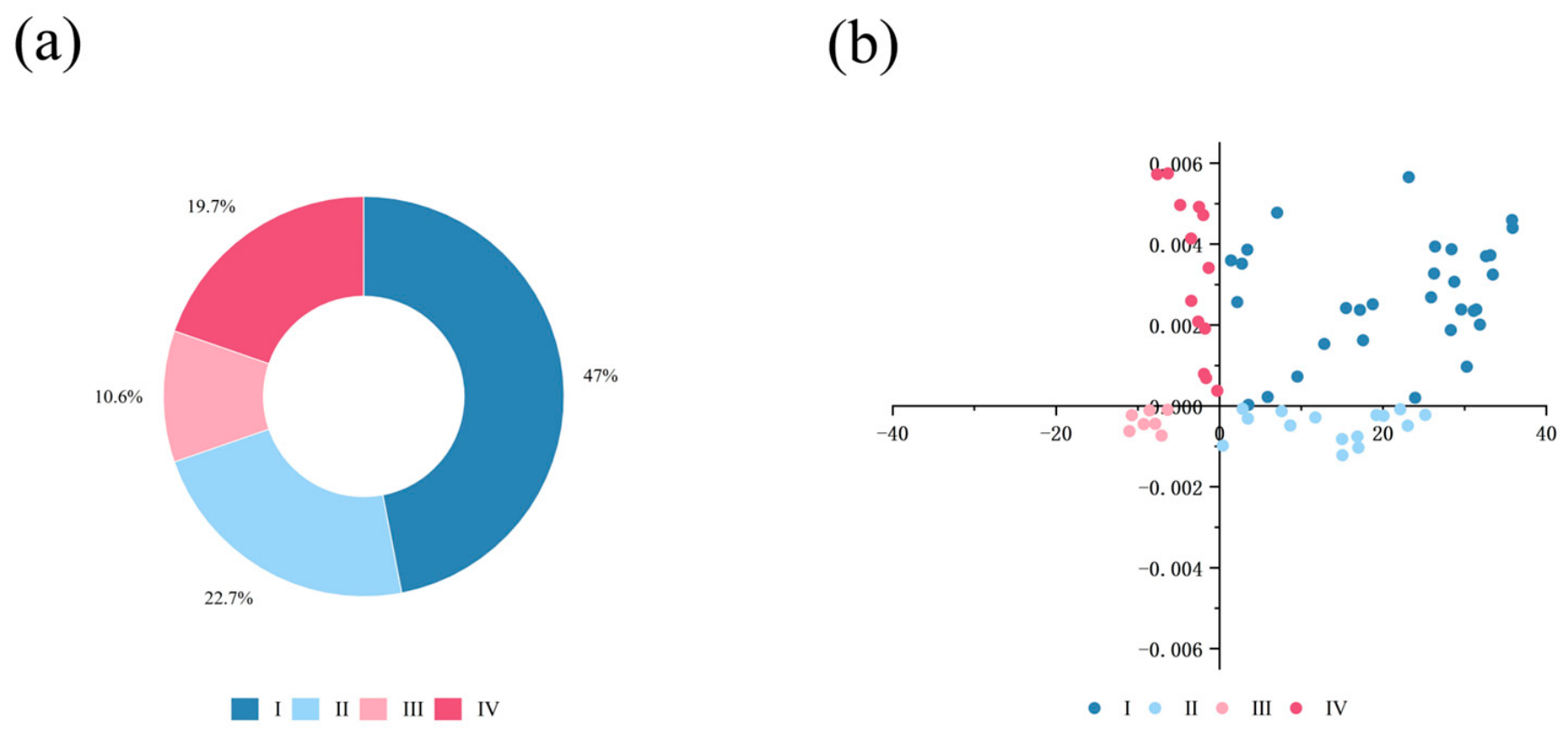
Transects were classified into four categories according to the signs of LRR (advance or retreat) and ΔFVC (increase or decrease): advance + increase, advance + decrease, retreat + increase, and retreat + decrease. The number and proportion of transects in each category were calculated. A four-category pie chart and a four-quadrant scatter plot were then used to display the distribution and directional consistency of the two variables, with LRR on the x-axis, ΔFVC on the y-axis, and reference lines at x = 0 and y = 0.

2.3.5. Spatial Autocorrelation Analysis

The midpoint of each transect was used as the spatial location. A K-nearest-neighbor method (K = 6) was used to construct a row-standardized spatial weight matrix.

(1) Global Moran’s I:

$$I={\displaystyle \frac{n}{S_0}}\cdot {\displaystyle \frac{{\sum }_i{\sum }_j{w}_{ij}\left(x_i-\overline{x}\right)\left(x_j-\overline{x}\right)}{{\sum }_i{\left(x_i-\overline{x}\right)}^2}}$$

(12)

where n = 66 is the number of transects, $w_{ij}$ is the spatial weight between transects i and j, $x_i$ and $x_j$ are the observed values at transects i and j, $\overline{x}$ is the mean value of the variable, and $S_0$ is the sum of all spatial weights.

(2) Local Moran’s I (Anselin Local Moran’s I):

$$I_i={\displaystyle \frac{x_i-\overline{x}}{m_2}}{\sum }_j{w}_{ij}\left(x_j-\overline{x}\right)$$

(13)

$I_i$ represents the local spatial association statistic for transect i. The results were classified into High–High (HH), Low–Low (LL), High–Low (HL), Low–High (LH), and non-significant categories.

The spatial autocorrelation analysis was performed in ArcGIS 10.8, and the significance level was set at α = 0.05.

3. Results

3.1. Spatiotemporal Changes in FVC

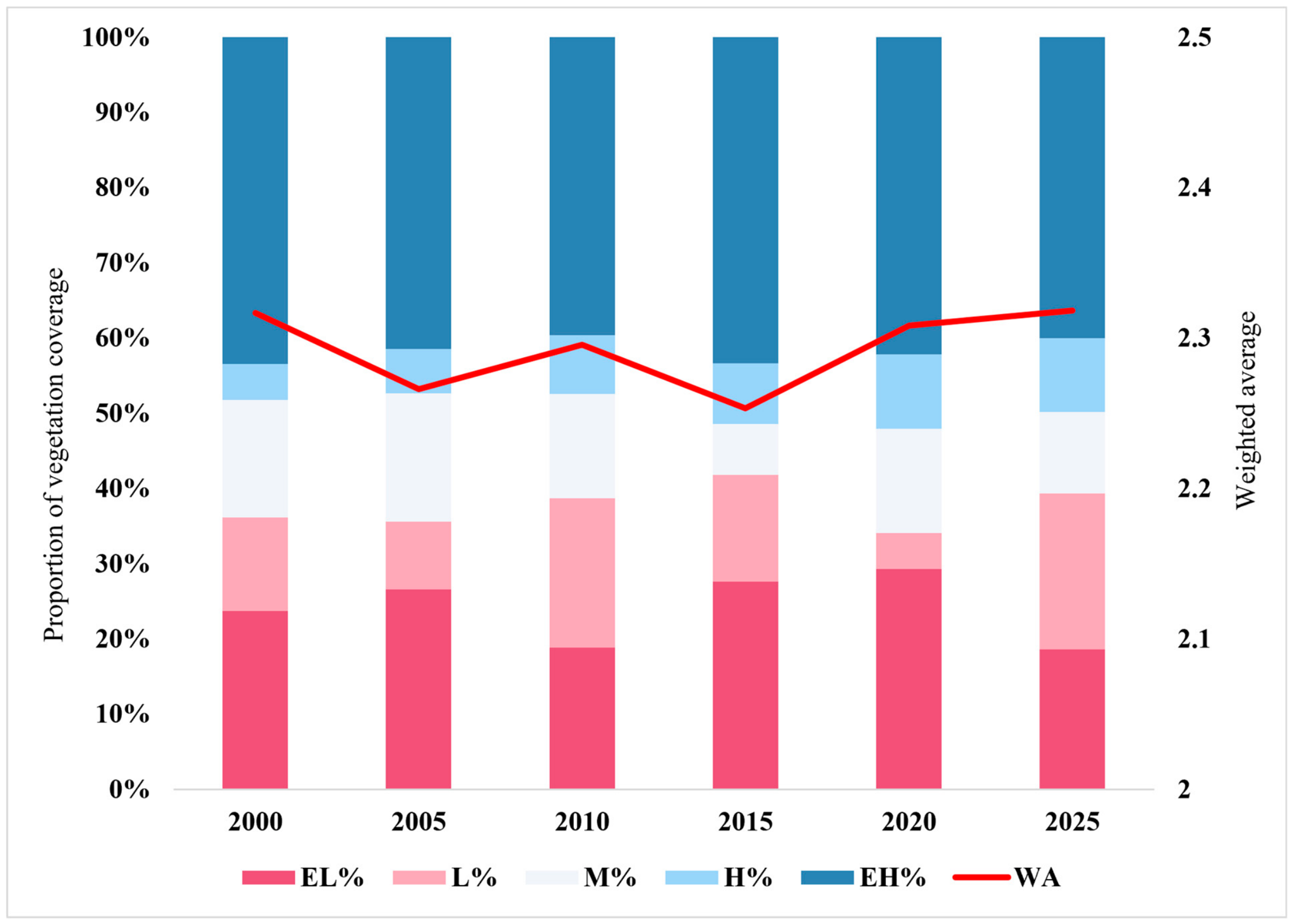
FVC was calculated using the pixel dichotomy model, and the area percentage of each FVC grade was summarized according to the classification standard in Table 3. Based on the weighted average method described in Section 2.3.2, WA was then calculated to represent the overall vegetation-cover status of the study area (Figure 4). From 2000 to 2025, the area percentages of the five FVC grades fluctuated over time. Extremely low cover (EL) ranged from 18.6% to 29.3%, low cover (L) from 4.8% to 20.8%, medium cover (M) from 6.8% to 17.1%, high cover (H) from 4.8% to 9.9%, and extremely high cover (EH) from 39.6% to 43.4%. Despite these interannual fluctuations in individual FVC classes, WA changed only slightly, from 2.317 in 2000 to 2.318 in 2025, with an overall interannual range of 0.065. This result indicates that the overall vegetation-cover status remained generally stable during the study period.

3.2. Vegetation Frontline Dynamics

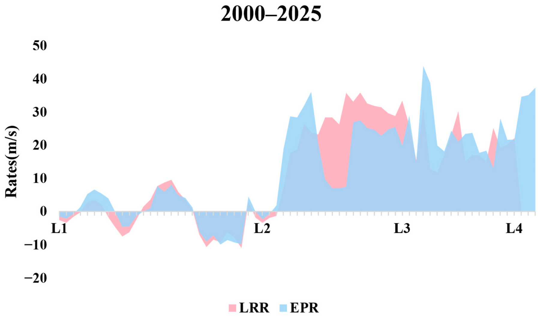
To characterize both the long-term trend of and short-term fluctuations in vegetation frontline migration, LRR and EPR were calculated for each transect using DSAS. The study area was divided into three sectors according to the spatial distribution of transects (Figure 5): L1–L2 (northern sector), L2–L3 (central sector), and L3–L4 (southern sector). Change rates were then summarized for each sector.

3.2.1. Long-Term Changes (2000–2025)

Long-term vegetation frontline change was quantified using LRR (

Table 4. Statistics of long-term (2000–2025) LRR and EPR values.

LONG TERM	Sector	Average Rates (m/yr)	Standard Deviation
2000–2025	EPR
	L1–L2	−0.56	5.73
	L2–L3	18.58	11.66
	L3–L4	25.22	8.60
	Entire	11.40	14.26
		LRR
	L1–L2	−1.45	5.86
	L2–L3	18.58	12.66
	L3–L4	25.22	6.59
	Entire	11.54	14.40

; Figure 6). The average LRR in the northern sector (L1–L2) was −1.45 m/yr, indicating retreat. In contrast, the central (L2–L3) and southern (L3–L4) sectors advanced at average rates of 18.58 m/yr and 25.22 m/yr, respectively. Across the entire study area, the average LRR was 11.54 m/yr, indicating a general seaward advance of approximately 11.5 m/yr over the 25-year period.

3.2.2. Short-Term Fluctuations (Every 5-Year Period)

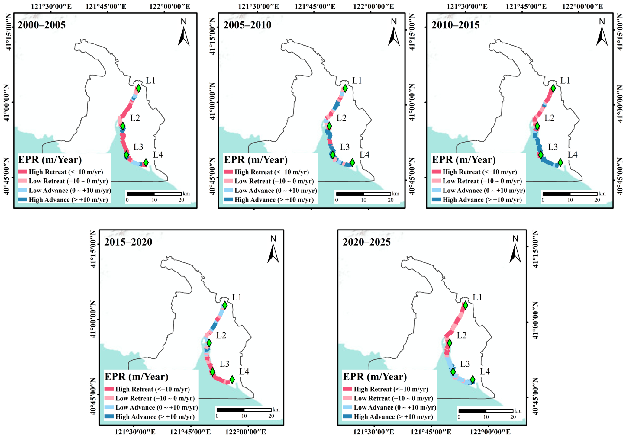
EPR was calculated for the five short-term intervals: 2000–2005, 2005–2010, 2010–2015, 2015–2020, and 2020–2025 (

Table 5. Statistics of the end point rate (EPR) for each short-term interval.

SHORT TERM	Sector	Average Rates (m/yr)	Standard Deviation
2000–2005	L1-L2	−13.97	20.93
	L2-L3	−51.38	155.68
	L3-L4	10.21	66.32
	Entire	−19.06	95.94
2005–2010	L1-L2	−1.18	14.63
	L2-L3	45.77	115.74
	L3-L4	26.52	29.11
	Entire	20.56	68.03
2010–2015	L1-L2	−12.36	7.96
	L2-L3	69.07	73.44
	L3-L4	63.88	39.75
	Entire	32.86	61.28
2015–2020	L1-L2	4.11	13.67
	L2-L3	−6.50	19.97
	L3-L4	−36.75	25.33
	Entire	−8.17	24.41
2020–2025	L1-L2	19.01	12.79
	L2-L3	61.33	47.49
	L3-L4	89.52	49.25
	Entire	50.16	51.97

; Figure 7). The results show pronounced short-term fluctuations and clear differences among sectors.

The study area retreated overall from 2000 to 2005 (−19.06 m/yr), shifted to advancing from 2005 to 2010 (20.56 m/yr), and advanced more strongly from 2010 to 2015 (32.86 m/yr). It retreated again from 2015 to 2020 (−8.17 m/yr) and then advanced sharply from 2020 to 2025 (50.16 m/yr). Large standard deviations in each interval indicate strong variability among transects. Sector-specific rates are listed in Table 5.

3.3. Spatial Comparison Between LRR and Least-Squares FVC Change Trends

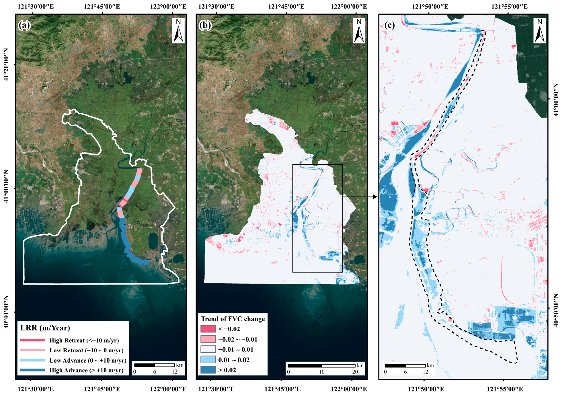
The linear slope of FVC change from 2000 to 2025 was calculated pixel by pixel using least-squares regression (b; unit: FVC/5 yr). Its spatial distribution is shown in Figure 8b,c.

A comparison between the FVC trend map (Figure 8b,c) and the LRR map (Figure 8a) shows that areas with positive b values, indicating FVC increase, largely overlap with clusters of positive LRR values, indicating frontline advance. Conversely, areas with negative b values tend to correspond to clusters of negative LRR values. This spatial correspondence suggests that the direction of vegetation frontline migration and the linear trend of FVC are broadly consistent.

3.4. Directional Consistency Between LRR and the Annual Change Rate of FVC (ΔFVC)

Because the regression step represents 5 years, the slope b was divided by 5 to obtain the annual change rate of FVC (ΔFVC; yr⁻¹). ΔFVC values were extracted to the 66 transect points in ArcGIS, and the transects were classified into four categories according to the signs of LRR and ΔFVC (Figure 9).

The four-category statistics (Figure 9a) show that 47.0% of transects (31 transects) exhibited simultaneous frontline advance and FVC increase, 22.7% (15 transects) showed advance but FVC decrease, 19.7% (13 transects) showed retreat but FVC increase, and 10.6% (seven transects) showed simultaneous retreat and FVC decrease. Thus, advance + increase was the dominant category, whereas the mismatch categories indicate that vegetation-cover response does not always occur synchronously with frontline migration. The four-quadrant scatter plot (Figure 9b) further illustrates this coupled but locally heterogeneous relationship.

3.5. Spatial Autocorrelation Analysis of LRR and ΔFVC

Global Moran’s I was used to examine the spatial autocorrelation of vegetation frontline change (LRR) and annual FVC change (ΔFVC) in the Liaohe Estuary wetland. The results are shown in

Table 6. Global spatial autocorrelation results for LRR and ΔFVC in the Liaohe Estuary wetland.

Indicator	Moran’s I	z-Score	p-Value	Spatial Autocorrelation Type
LRR	0.8754	13.2354	<0.001	extremely significant positive spatial autocorrelation
ΔFVC	0.6139	9.3622	<0.001	extremely significant positive spatial autocorrelation

.

The Global Moran’s I value of LRR was 0.875 (z = 13.24, p < 0.001), and that of ΔFVC was 0.614 (z = 9.36, p < 0.001). These results indicate that both variables exhibited extremely significant positive spatial autocorrelation.

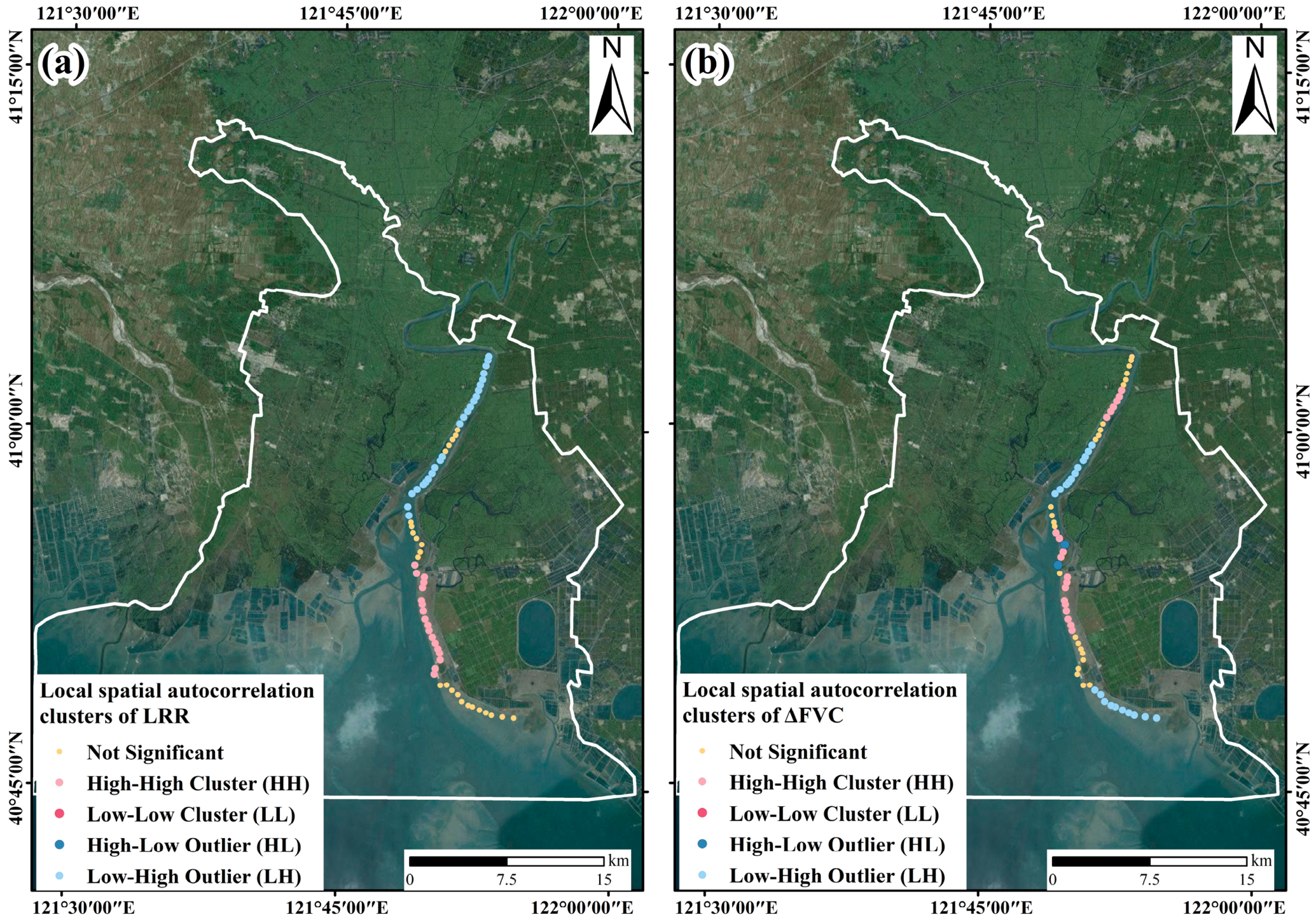
The Local Moran’s I cluster maps (Figure 10) show that the High–High (HH) clusters of LRR are mainly distributed in the central and southern coastal sections. The HH clusters of ΔFVC also occur mainly in the central and southern sections, with several additional clusters in the north. Therefore, the two variables show broad spatial correspondence but do not completely overlap locally.

3.6. Vegetation Classification Results and Accuracy Assessment

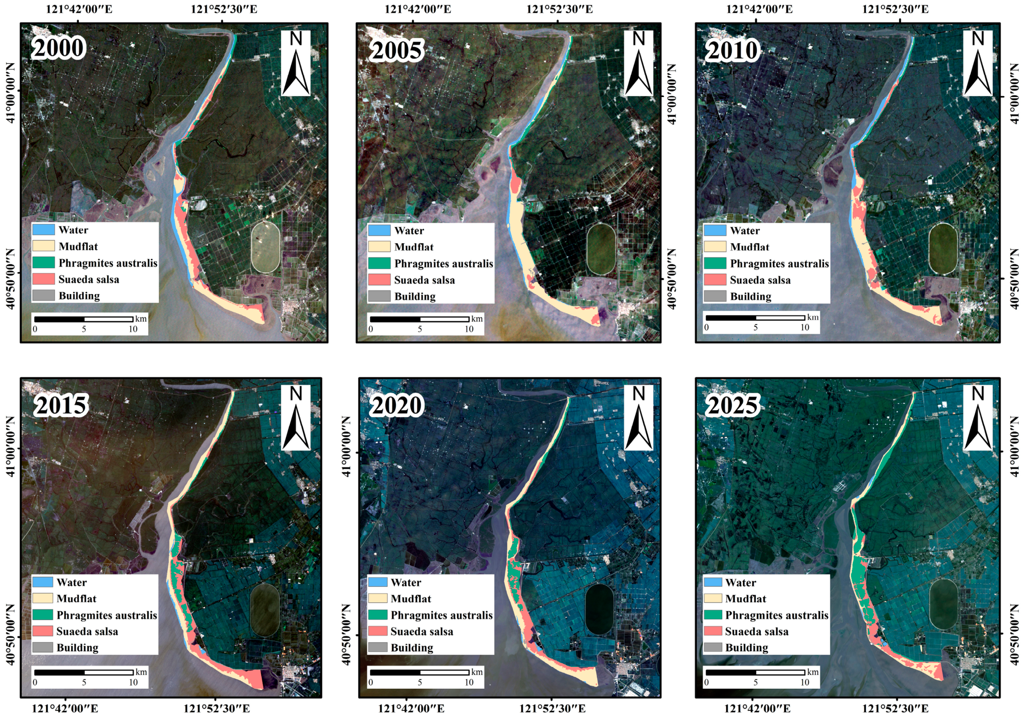
The spatial distribution of the six land-cover classification maps from 2000 to 2025 is shown in Figure 11. The main land-cover types are water body, mudflat, Suaeda salsa, Phragmites australis, and a small amount of built-up land.

The reliability of the eCognition-based multi-scale segmentation and threshold segmentation classification was assessed using a confusion matrix for each image period. For each period, 180 validation points with a minimum spacing of 50 m were randomly generated. Actual land-cover types were determined by visual interpretation of high-resolution imagery, and OA and the Kappa coefficient were calculated. The results are shown in

Table 7. Statistics of vegetation classification accuracy for each phase.

Year	Overall Accuracy (OA)	Kappa Coefficient
2000	92.78%	0.8943
2005	89.44%	0.8123
2010	92.22%	0.8828
2015	95.05%	0.9245
2020	92.78%	0.8896
2025	92.78%	0.8919

.

The six land-cover classifications achieved OA values of 89.4–95.1% and Kappa coefficients of 0.812–0.925, indicating high agreement with the validation data. These results support the use of the classification outputs in the subsequent vegetation-conversion analysis.

3.7. Short-Term Vegetation Frontline Fluctuations and Vegetation-Type Conversion

The relationship between short-term frontline fluctuation and community succession was analyzed using EPR for the five 5-year intervals (Table 5) and the vegetation-type conversion chord diagrams (Figure 12). As described in Section 3.2.2, EPR showed periodic fluctuations: retreat in 2000–2005 (−19.06 m/yr), rapid advance in 2005–2015 (20.56–32.86 m/yr), renewed retreat in 2015–2020 (−8.17 m/yr), and sharp advance in 2020–2025 (50.16 m/yr).

The chord diagrams (Figure 12) show clear differences in vegetation-type conversion among the five intervals. From 2000 to 2005, the widest conversion pathway was Suaeda salsa → mudflat. From 2005 to 2010, mudflat → Suaeda salsa conversion began to increase. From 2010 to 2015, mudflat → Suaeda salsa and Suaeda salsa → Phragmites australis pathways were strengthened. From 2015 to 2020, partial reverse conversion from Phragmites australis or Suaeda salsa to mudflat indicated localized degradation. From 2020 to 2025, the conversion from Suaeda salsa to Phragmites australis increased markedly, consistent with rapid succession under continued frontline advance.

4. Discussion

4.1. Study-Area Focus: The Eastern Bank of the Liaohe Estuary

The results show that WA, defined as the weighted average of the five FVC classes, fluctuated only within a narrow range of 2.25–2.32 from 2000 to 2025, indicating generally stable vegetation-cover status at the whole-area scale. A comparison between the eastern and western coasts of the Liaohe Estuary helps explain the focus of this study. The western coast has long been occupied by dense aquaculture enclosures, which disrupt tidal hydrological connectivity and restrict natural sediment transport. The vegetation dynamics there are therefore strongly affected by cumulative anthropogenic stress. By contrast, the eastern coast has experienced relatively less artificial disturbance, and its tidal-creek system remains comparatively well preserved. This setting provides a more suitable background for analyzing coupled relationships among vegetation frontline advance or retreat, sediment accretion, and vegetation succession. The uniformly spaced transects on the eastern coast and the complete time series further support spatial coupling analysis between vegetation frontline dynamics and FVC change. For these reasons, the discussion focuses on the eastern bank of the Liaohe Estuary and on the geomorphology–vegetation feedback operating there [34].

4.2. Stage Characteristics of Vegetation Frontline Dynamics and Their Geomorphological Implications

From 2000 to 2025, the vegetation frontline on the eastern bank of the Liaohe Estuary followed a three-stage trajectory: retreat, slow advance, and rapid expansion. The long-term LRR was +11.5 m/yr, indicating net seaward expansion. In contrast, the short-term EPR values fluctuated strongly, ranging from −19.1 m/yr in 2000–2005 to +50.2 m/yr in 2020–2025. This contrast between the long-term trend and short-term variability reflects the sensitivity of tidal-flat geomorphology to sediment supply and tidal dynamics [35]. During 2000–2005, reduced sediment input from the river basin and changes in regional water-sediment conditions associated with aquaculture activities along adjacent shorelines likely reduced net sediment supply to the tidal flat [36,37]. Net erosion consequently dominated, leading to landward retreat of the vegetation frontline. During 2005–2015, localized aquaculture-pond restoration and tidal-creek dredging partially restored tidal connectivity [38], allowing net sediment deposition to become increasingly important and causing slow seaward advance. After 2015, larger-scale ecological restoration, especially tidal-creek dredging, enhanced tidal sediment transport and increased net deposition, driving rapid seaward expansion of the vegetation frontline [39,40].

4.3. Hypothesized Coupling Among Frontline Expansion, Elevation Rise, and Vegetation Succession

The successional sequence revealed by the chord diagrams (Figure 12) was highly synchronized with periodic changes in EPR. Specifically, the dominant pathway was Suaeda salsa → mudflat during degradation in 2000–2005, mudflat → Suaeda salsa during recovery in 2005–2015, and Suaeda salsa → Phragmites australis expansion during succession in 2015–2025. Based on these patterns, we propose the following conceptual hypothesis, consistent with salt-marsh ecogeomorphology theory: vegetation frontline progradation enhances sediment accumulation, raises tidal-flat elevation, reduces inundation frequency and salinity, promotes Suaeda salsa colonization, and eventually facilitates Phragmites australis expansion. This interpretation is ecologically plausible but requires direct validation through sedimentological and topographic field measurements. Therefore, the inferred causal links should be understood as hypotheses rather than demonstrated causal mechanisms.

This sequence is consistent with a positive feedback mechanism linking frontline dynamics, sedimentation or erosion, elevation change, and habitat filtering in salt-marsh ecogeomorphology. Existing studies suggest that Suaeda salsa, as a pioneer species, is adapted to relatively low elevations and high soil salinity [41,42]. By contrast, Phragmites australis generally occupies higher elevations with less frequent inundation and lower salinity. Therefore, changes in the rate of vegetation frontline migration can be interpreted as an indirect indicator of sedimentation processes.

• Low-sedimentation stage, corresponding to the retreat period of 2000–2005: The vegetation frontline retreated overall, indicating net erosion, decreasing or stagnant tidal-flat elevation, prolonged inundation, and relatively high salinity [43,44]. Habitat conditions likely moved beyond the suitable range for Suaeda salsa, leading to vegetation degradation. Accordingly, Suaeda salsa → mudflat was the dominant conversion pathway in the chord diagram.
• Medium-sedimentation stage, corresponding to the slow-advance period of 2005–2015: The frontline shifted to gradual seaward advance, net sedimentation began to dominate, and elevation likely increased gradually. As inundation duration shortened and salinity decreased, habitats became more suitable for Suaeda salsa, leading to increased mudflat → Suaeda salsa conversion in the chord diagram.
• High-sedimentation stage, corresponding to the rapid-advance period of 2015–2025 and especially the extremely rapid advance in 2020–2025: The frontline expanded rapidly seaward, net sedimentation increased, and elevation likely rose quickly. Shorter inundation duration and lower salinity may have pushed habitat conditions beyond the upper suitable range of Suaeda salsa and toward conditions favorable for Phragmites australis. Because of its stronger competitive ability, Phragmites australis may have gradually replaced Suaeda salsa, which is consistent with the enhanced Suaeda salsa → Phragmites australis conversion shown by the chord diagram.

The “spatial mismatch” revealed by the Local Moran’s I analysis (Figure 10) also supports this interpretation. HH clusters of LRR were mainly distributed in the central and southern coastal sections, whereas HH clusters of ΔFVC were concentrated in the central and southern sections with several additional northern clusters. At the macro scale, the central and southern sections were both the core areas of rapid frontline advance and the dominant areas of FVC increase. Locally, however, the two cluster patterns did not coincide completely. Newly formed tidal flats in rapidly advancing zones may still be in an early successional stage, so FVC increase can lag behind Suaeda salsa colonization. In more mature successional zones, Phragmites australis expansion may already have produced higher ΔFVC values. Thus, the partial mismatch between LRR and ΔFVC clusters reflects the time lag between elevation accumulation and vegetation response [45,46,47].

This mismatch indicates that the frontline-advance rate is not by itself a direct predictor of FVC change. Instead, the time lag between elevation evolution and vegetation response is critical for interpreting their spatial coupling.

Although elevation change is central to the conceptual model proposed here, other drivers may also contribute to the observed Suaeda salsa → Phragmites australis transition. Freshwater input from upstream river discharge can lower soil salinity and thereby favor Phragmites australis over Suaeda salsa [48,49]. Nutrient enrichment, potentially associated with agricultural runoff in the surrounding basin, may also promote Phragmites expansion [50]. In addition, interspecific competition and litter-mediated shading may further increase the competitive advantage of Phragmites australis and accelerate community replacement [51]. Because in situ measurements of salinity, nutrient concentrations, and light availability are not available, these alternative drivers cannot be excluded. Future field studies should measure these variables to distinguish their relative contributions. Nevertheless, the strong spatial association between vegetation frontline advance, used here as an indirect proxy for accretion, and succession patterns suggests that elevation change remains an important control.

4.4. Strengthening Effect of Ecological Restoration on Geomorphology–Vegetation Positive Feedback

Large-scale ecological restoration after 2015, including tidal-creek dredging, appears to have strengthened the geomorphology–vegetation positive feedback described above. Restoration of the tidal-creek system likely improved tidal sediment transport efficiency and increased net accretion. Microtopographic modification may also have enhanced seed retention, thereby promoting vegetation establishment and succession.

However, the extremely rapid progradation during 2020–2025 was accompanied by rapid replacement of Suaeda salsa by Phragmites australis and rapid expansion of the latter. Although this shift can improve shoreline stabilization and carbon sequestration, it may also reduce plant diversity and promote a single-dominant-species pattern. Future management should therefore regulate artificial sediment-enhancement intensity and retain local low-elevation areas where appropriate. Such measures would help maintain Suaeda salsa habitats and preserve community structural heterogeneity and ecological functional diversity.

4.5. Management Implications and Research Limitations

Based on the above findings, the following management recommendations are proposed:

First, management zoning should consider elevation regulation. In the Liaohe Estuary, coastal wetland elevations generally range from 1.3 to 4.0 m [19]. Previous field measurements in the delta show that Phragmites australis marshes occupy higher surface elevations and have significantly greater vertical accretion rates than Suaeda salsa marshes [18], consistent with the elevation partitioning indicated by the land-cover classification in this study. Accordingly, Suaeda salsa communities should be maintained or restored in relatively low-elevation areas to avoid excessive rapid accretion [52], whereas Phragmites australis development can be guided in higher-elevation areas to create a heterogeneous landscape [53,54]. These elevation values are site-specific empirical references for the Liaohe Estuary rather than universal thresholds; therefore, field validation, such as real-time kinematic global positioning system (RTK-GPS) surveys, is required before applying them to other estuaries.

Second, progradation rate should be incorporated into restoration planning. In areas where the vegetation frontline advances rapidly, managers should account for the lagged vegetation response. A 1–2-year establishment window may be reserved, and artificial seeding can be applied when natural colonization is insufficient.

Third, long-term coupled monitoring should be strengthened. A fixed-point observation network for tidal-flat elevation and vegetation cover is recommended to validate succession models and to support adaptive management.

This study has several limitations. The 5-year temporal resolution cannot capture intra-annual storm events or seasonal tidal variations, and the relative contributions of riverine sediment discharge and sea-level rise to accretion are not quantitatively separated. Future research should integrate higher-frequency remote-sensing data, such as Sentinel-2 imagery, with in situ hydrodynamic and geomorphological observations to construct a multi-factor driving model.

4.6. Limitations Related to Temporal Data Characteristics

A potential concern is that the three-week offset between early-September images (2000 and 2005) and late-September images (2010–2025) could artificially produce the observed retreat–advance–expansion pattern. Several lines of evidence suggest that this is unlikely.

First, the magnitude of the observed changes is much larger than any plausible phenological effect. The measured retreat from 2000 to 2005 averaged −19.1 m/yr, and the advance from 2020 to 2025 reached +50.2 m/yr. Any positional shift caused by phenological differences in canopy cover or NDVI would likely be much smaller than these rates, as also suggested by the stable vegetation–mudflat boundary observed in the field (Figure S1). Therefore, the three-stage pattern cannot be explained solely by acquisition-date variation.

Second, the Otsu thresholds remained stable (0.20–0.25) across all six time points (Table 2), indicating that the spectral contrast between vegetation and non-vegetation did not change systematically between early and late September. If phenological degradation had strongly affected the imagery, the optimal thresholds would have shifted toward lower values in late September, which was not observed.

Third, the strong spatial autocorrelation (Global Moran’s I = 0.875 for LRR and 0.614 for ΔFVC, both p < 0.001) and high classification accuracy (OA > 89%, Kappa > 0.81) provide internal consistency evidence that would be unlikely if the observed signal was dominated by date-related artifacts.

Fourth, the vegetation-conversion chord diagrams (Figure 12) are logically synchronized with EPR directions: retreat intervals show Suaeda salsa → mudflat conversion, whereas advance intervals show mudflat → Suaeda salsa and Suaeda salsa → Phragmites australis conversion. This synchrony would be unlikely if the results were mainly caused by phenological timing differences.

Therefore, the observed three-stage pattern is interpreted as a genuine ecological succession process rather than a phenological artifact. Although identical acquisition dates would be ideal, the current dataset is sufficient to support the main conclusions. Future studies using a more consistent phenological window could refine the absolute rates but are unlikely to reverse the directional trends.

In addition, this study relies on six discrete remote-sensing time points (2000, 2005, 2010, 2015, 2020, and 2025) at 5-year intervals. Although this temporal resolution captures decadal trends, it cannot resolve intra-annual storm events, seasonal tidal variations, or rapid ecological transitions. Future work should integrate higher-frequency time series, such as Sentinel-2 imagery, to capture continuous trajectories and validate the stage boundaries identified here.

5. Conclusions

• The vegetation frontline showed stage-wise evolution, and ecological restoration contributed to rapid expansion in the later period. From 2000 to 2025, the vegetation frontline on the eastern bank of the Liaohe Estuary followed a three-stage pattern of retreat, slow advance, and rapid expansion. The long-term LRR was +11.5 m/yr, indicating net seaward expansion, whereas the short-term EPR fluctuated from −19.1 m/yr in 2000–2005 to +50.2 m/yr in 2020–2025. Large-scale ecological restoration, especially tidal-creek dredging after 2015, likely increased net sediment deposition and became an important driver of rapid seaward frontline expansion.
• Frontline expansion and vegetation succession were coupled stage-wise. The chord diagrams were synchronized with periodic EPR changes: during frontline retreat in 2000–2005, the dominant conversion was Suaeda salsa → mudflat, indicating degradation; during slow advance in 2005–2015, the dominant conversion was mudflat → Suaeda salsa, indicating recovery; and during rapid advance in 2015–2025, the dominant conversions were Suaeda salsa → Phragmites australis succession and Phragmites expansion. This sequence suggests that sediment deposition associated with frontline advance raised tidal-flat elevation and promoted stagewise salt-marsh vegetation succession, consistent with ecogeomorphological positive feedback.
• LRR and ΔFVC showed significant positive spatial autocorrelation but also local spatial mismatch caused by succession lag. Global Moran’s I indicated extremely significant positive spatial autocorrelation for both variables (LRR = 0.875; ΔFVC = 0.614; p < 0.001). In the Local Moran’s I cluster maps, HH clusters of LRR and ΔFVC were both concentrated mainly in the central and southern sections but did not completely overlap, indicating that vegetation-cover response lagged behind rapid frontline advance in some areas.
• Ecological restoration strengthened geomorphology–vegetation positive feedback, but the risk of Phragmites australis dominance requires attention. Restoration projects accelerated sedimentation and compressed the succession timescale to approximately 5–10 years. However, very rapid advance has promoted the expansion of Phragmites australis, which may reduce Suaeda salsa habitat and landscape heterogeneity.
• This study provides support for zone-specific regulation and rate-sensitive management in estuarine wetlands. In low-elevation areas, Suaeda salsa communities should be maintained or restored to avoid excessive rapid sedimentation; in high-elevation areas, Phragmites australis communities can be guided to create a heterogeneous landscape. In areas with rapid frontline advance, a 1–2-year vegetation-establishment window should be reserved, with artificial seeding as a supplement when necessary. A fixed-point observation network for tidal-flat elevation and FVC is recommended to validate succession models.

Overall, these management recommendations support the sustainable development of the Liaohe Estuary wetland ecosystem by providing science-based zoning guidance and restoration timing strategies. The integrated remote-sensing approach demonstrated in this study offers a replicable framework for sustainability assessment and long-term monitoring of other coastal wetlands facing similar environmental pressures.

References

1. Phillips, A.; Bastola, S. Assessing Vegetation and Shoreline Responses in Reduced Wave Climates Using Google Imagery. J. Coast. Res. 2025, 41, 950–966. [Google Scholar] [CrossRef]
2. Hill, M.J.; Guerschman, J.P. Global Trends in Vegetation Fractional Cover: Hotspots for Change in Bare Soil and Non-Photosynthetic Vegetation. Agric. Ecosyst. Environ. 2022, 324, 107719. [Google Scholar] [CrossRef]
3. Cui, P.; Su, F.; Zhou, F. Inundation Depth Shape Phenotypic Variability of Phragmites australis in Liaohe Estuary Wetland, Northeast China. Sustainability 2022, 14, 14911. [Google Scholar] [CrossRef]
4. Li, H.; Wang, L.; Su, F.; Xiao, C.; Yan, M.; Song, F. Research on Typical Estuarine Sedimentation Characteristics: A Case Study of the Liaohe Estuary Wetland. Sustainability 2025, 17, 8410. [Google Scholar] [CrossRef]
5. Li, W.; Liu, L.; Zhu, W.; Li, J.; Liu, T. Shoreline_veget—A New Shoreline Extraction Method for Vegetation Seas, with High Robustness, Accuracy and Scalability. Front. Mar. Sci. 2025, 12, 1491085. [Google Scholar] [CrossRef]
6. Foggi Rota, G.; Tressoldi, E.; Avallone, F.; Rosti, M.E. Edge Effects in the Turbulent Flow over Flexible Aquatic Vegetation. J. Fluid Mech. 2025, 1019, A45. [Google Scholar] [CrossRef]
7. Villoslada, M.; Sipelgas, L.; Bergamo, T.F.; Ward, R.D.; Reintam, E.; Astover, A.; Kumpula, T.; Sepp, K. Multi-Source Remote Sensing Data Reveals Complex Topsoil Organic Carbon Dynamics in Coastal Wetlands. Ecol. Indic. 2022, 143, 109329. [Google Scholar] [CrossRef]
8. Martínez-Sánchez, A.; Gracia, F.J.; Alonso, C.; Mata, E.; Caporizzo, C. Reconstructing the Historical Shoreline Evolution of the Northern Bay of Cádiz (SW Spain) from Geomorphological and Geoarchaeological Data. J. Maps 2023, 19, 2206585. [Google Scholar] [CrossRef]
9. Abd-Elhamid, H.F.; Zeleňáková, M.; Barańczuk, J.; Gergelova, M.B.; Mahdy, M. Historical Trend Analysis and Forecasting of Shoreline Change at the Nile Delta Using RS Data and GIS with the DSAS Tool. Remote Sens. 2023, 15, 1737. [Google Scholar] [CrossRef]
10. Daramola, S.; Li, H.; Otoo, E.; Idowu, T.; Gong, Z. Coastal Evolution Assessment and Prediction Using Remotely Sensed Front Vegetation Line along the Nigerian Transgressive Mahin Mud Coast. Reg. Stud. Mar. Sci. 2022, 50, 102167. [Google Scholar] [CrossRef]
11. Khurram, S.; Pour, A.B.; Bagheri, M.; Helmy Ariffin, E.; Akhir, M.F.; Bahri Hamzah, S. Satellite-Based Multi-Decadal Shoreline Change Detection by Integrating Deep Learning with DSAS: Eastern and Southern Coastal Regions of Peninsular Malaysia. Remote Sens. 2025, 17, 3334. [Google Scholar] [CrossRef]
12. Lin, P.; Wei, X.; Zhang, Y.; Lv, P.; Liu, M.; Yang, Y.; Dong, X. Quantifying Spatiotemporal Evolution of Sandy Shorelines in Northern China Using DSAS: A Case Study from Dalian World Peace Park. Sustainability 2025, 17, 7591. [Google Scholar] [CrossRef]
13. Memisoglu Baykal, T. Performance Assessment of GIS-Based Spatial Clustering Methods in Forest Fire Data. Nat. Hazards 2025, 121, 8445–8477. [Google Scholar] [CrossRef]
14. Kirwan, M.L.; Megonigal, J.P. Tidal Wetland Stability in the Face of Human Impacts and Sea-Level Rise. Nature 2013, 504, 53–60. [Google Scholar] [CrossRef] [PubMed]
15. Leonardi, N.; Fagherazzi, S. How Waves Shape Salt Marshes. Geology 2014, 42, 887–890. [Google Scholar] [CrossRef]
16. Mariotti, G.; Fagherazzi, S. A Numerical Model for the Coupled Long-term Evolution of Salt Marshes and Tidal Flats. J. Geophys. Res. Earth Surf. 2010, 115, 2009JF001326. [Google Scholar] [CrossRef]
17. Hu, K.; Chen, Q.; Wang, H.; Hartig, E.K.; Orton, P.M. Numerical Modeling of Salt Marsh Morphological Change Induced by Hurricane Sandy. Coast. Eng. 2018, 132, 63–81. [Google Scholar] [CrossRef]
18. Wang, G.; Wang, M.; Lu, X.; Jiang, M. Surface Elevation Change and Susceptibility of Coastal Wetlands to Sea Level Rise in Liaohe Delta, China. Estuar. Coast. Shelf Sci. 2016, 180, 204–211. [Google Scholar] [CrossRef]
19. Zhang, Y.; Yu, W.; Ji, R.; Zhao, Y.; Feng, R.; Jia, Q.; Wu, J. Dynamic Response of Phragmites australis and Suaeda salsa to Climate Change in the Liaohe Delta Wetland. J. Meteorol. Res. 2021, 35, 157–171. [Google Scholar] [CrossRef]
20. Howes, N.C.; FitzGerald, D.M.; Hughes, Z.J.; Georgiou, I.Y.; Kulp, M.A.; Miner, M.D.; Smith, J.M.; Barras, J.A. Hurricane-Induced Failure of Low Salinity Wetlands. Proc. Natl. Acad. Sci. USA 2010, 107, 14014–14019. [Google Scholar] [CrossRef] [PubMed]
21. Feagin, R.A.; Lozada-Bernard, S.M.; Ravens, T.M.; Möller, I.; Yeager, K.M.; Baird, A.H. Does Vegetation Prevent Wave Erosion of Salt Marsh Edges? Proc. Natl. Acad. Sci. USA 2009, 106, 10109–10113. [Google Scholar] [CrossRef] [PubMed]
22. Ren, L.; Zhang, S.; Guo, X.; Cheng, L.; Guo, Y.; Ding, A. Interannual Variation in Riparian Vegetation Cover and Its Relationship with River Flow under a High Level of Human Intervention: An Example from the Yongding River Basin. Environ. Monit. Assess. 2021, 193, 406. [Google Scholar] [CrossRef] [PubMed]
23. Su, F.; Liu, H.; Zhu, D.; Li, L.; Wang, T. Sustainability Assessment of the Liaohe Estuary Wetland Based on Emergy Analysis. Ecol. Indic. 2020, 119, 106837. [Google Scholar] [CrossRef]
24. Li, X.; Anderson, C.J.; Wang, Y.; Lei, G. Waterbird Diversity and Abundance in Response to Variations in Climate in the Liaohe Estuary, China. Ecol. Indic. 2021, 132, 108286. [Google Scholar] [CrossRef]
25. Yang, X.; Zheng, D.; Sun, Y. Evolution and Vulnerability Assessment of Wetland Landscape Pattern in the Liaohe Estuary Over the Past 35 Years. Wetlands 2026, 46, 15. [Google Scholar] [CrossRef]
26. Cao, C.; Su, F.; Song, F.; Yan, H.; Pang, Q. Distribution and Disturbance Dynamics of Habitats Suitable for Suaeda salsa. Ecol. Indic. 2022, 140, 108984. [Google Scholar] [CrossRef]
27. Ke, Y.; Han, Y.; Cui, L.; Sun, P.; Min, Y.; Wang, Z.; Zhuo, Z.; Zhou, Q.; Yin, X.; Zhou, D. Suaeda salsa Spectral Index for Suaeda salsa Mapping and Fractional Cover Estimation in Intertidal Wetlands. ISPRS J. Photogramm. Remote Sens. 2024, 207, 104–121. [Google Scholar] [CrossRef]
28. Liu, L.; Wang, Z.; Wang, Y.; Zhang, Y.; Shen, J.; Qin, D.; Li, S. Trade-off Analyses of Multiple Mountain Ecosystem Services along Elevation, Vegetation Cover and Precipitation Gradients: A Case Study in the Taihang Mountains. Ecol. Indic. 2019, 103, 94–104. [Google Scholar] [CrossRef]
29. Xiang, Z.; Liu, Y.; Fu, Y.; Gao, Y.; Liu, L.; Wang, F. Spatiotemporal Change Characteristics of NDVI and Response to Climate Factors in the Jixi Wetland, Eastern China. Environ. Monit. Assess. 2024, 196, 808. [Google Scholar] [CrossRef] [PubMed]
30. Duarte, A.; Acevedo-Muñoz, L.; Gonçalves, C.I.; Mota, L.; Sarmento, A.; Silva, M.; Fabres, S.; Borralho, N.; Valente, C. Detection of Longhorned Borer Attack and Assessment in Eucalyptus Plantations Using UAV Imagery. Remote Sens. 2020, 12, 3153. [Google Scholar] [CrossRef]
31. Duo, A.; Zhao, W.; Qu, X.; Jing, R.; Xiong, K. Spatio-Temporal Variation of Vegetation Coverage and Its Response to Climate Change in North China Plain in the Last 33 Years. Int. J. Appl. Earth Obs. Geoinf. 2016, 53, 103–117. [Google Scholar] [CrossRef]
32. Wang, R.; Wang, H.; Wang, C.; Duan, J.; Zhang, S. Spatial Scale Effect on Fractional Vegetation Coverage Changes and Driving Factors in the Henan Section of the Yellow River Basin. Remote Sens. 2024, 16, 2575. [Google Scholar] [CrossRef]
33. Chabalala, Y.; Adam, E.; Ali, K.A. Machine Learning Classification of Fused Sentinel-1 and Sentinel-2 Image Data towards Mapping Fruit Plantations in Highly Heterogenous Landscapes. Remote Sens. 2022, 14, 2621. [Google Scholar] [CrossRef]
34. Brown, D.R.; Conrad, S.; Akkerman, K.; Fairfax, S.; Fredericks, J.; Hanrio, E.; Sanders, L.M.; Scott, E.; Skillington, A.; Tucker, J.; et al. Seagrass, Mangrove and Saltmarsh Sedimentary Carbon Stocks in an Urban Estuary; Coffs Harbour, Australia. Reg. Stud. Mar. Sci. 2016, 8, 1–6. [Google Scholar] [CrossRef]
35. Zhou, Z.; Grandjean, T.J.; De Smit, J.; Van Belzen, J.; Fivash, G.S.; Walles, B.; Beauchard, O.; Van Dalen, J.; Blok, D.B.; Van IJzerloo, L.; et al. Sediment Dynamics Shape Macrofauna Mobility Traits and Abundance on Tidal Flats. Limnol. Oceanogr. 2024, 69, 2278–2293. [Google Scholar] [CrossRef]
36. Wang, D.; Zhou, T.; Fan, J.; Tang, Z.; Wang, Y. Evolution Trend and Cause Analysis of Diversion Characteristics of Three Outlets Along Jingjiang River Under New Flow and Sediment Conditions. Sustainability 2025, 17, 8285. [Google Scholar] [CrossRef]
37. Wu, J.; Liu, L.; Chen, J.; Chen, G.; Zhu, H.; Liu, J.; Ye, Y. Effects of Dredging Wastewater Input History and Aquaculture Type on Greenhouse Gas Fluxes from Mangrove Sediments along the Shorelines of the Jiulong River Estuary, China. Environ. Pollut. 2024, 346, 123672. [Google Scholar] [CrossRef] [PubMed]
38. Fleri, J.R.; Lera, S.; Gerevini, A.; Staver, L.; Nardin, W. Empirical Observations and Numerical Modelling of Tides, Channel Morphology, and Vegetative Effects on Accretion in a Restored Tidal Marsh. Earth Surf. Process. Landf. 2019, 44, 2223–2235. [Google Scholar] [CrossRef]
39. Fan, X.; Huang, H.; Zhang, Q.; Sun, N.; Wang, Y. Response of Tidal Creek Networks and Tidal Connectivity to Coastal Squeeze of Saltmarshes in the Southern Bohai Bay. N. Z. J. Mar. Freshw. Res. 2022, 56, 617–631. [Google Scholar] [CrossRef]
40. Khadanga, M.K.; Mishra, R.K.; Sahoo, R.K.; Dora, D.P.; Behera, A.K.; Panda, U.S.; Mohanty, P.K.; Mishra, P. Seagrass Conservation in a Dynamic Tidal Creek System: Balancing Creek Stability and Nutrient Loads for Sustainable Management. Sci. Total Environ. 2025, 1001, 180462. [Google Scholar] [CrossRef] [PubMed]
41. Zhang, Q.-H.; Sairebieli, K.; Zhao, M.-M.; Sun, X.-H.; Wang, W.; Yu, X.-N.; Du, N.; Guo, W.-H. Nutrients Have a Different Impact on the Salt Tolerance of Two Coexisting Suaeda Species in the Yellow River Delta. Wetlands 2020, 40, 2811–2823. [Google Scholar] [CrossRef]
42. Wang, N.; Zhao, Z.; Zhang, X.; Liu, S.; Zhang, K.; Hu, M. Plant Growth, Salt Removal Capacity, and Forage Nutritive Value of the Annual Euhalophyte Suaeda salsa Irrigated with Saline Water. Front. Plant Sci. 2023, 13, 1040520. [Google Scholar] [CrossRef] [PubMed]
43. Zhang, X.; Zuo, L.; Lu, Y.; Li, H.; Zhao, Y. An Improved Approach for Retrieval of Tidal Flat Elevation Based on Inundation Frequency. Estuar. Coast. Shelf Sci. 2025, 313, 109061. [Google Scholar] [CrossRef]
44. Kauffman, J.B.; Giovanonni, L.; Kelly, J.; Dunstan, N.; Borde, A.; Diefenderfer, H.; Cornu, C.; Janousek, C.; Apple, J.; Brophy, L. Total Ecosystem Carbon Stocks at the Marine-terrestrial Interface: Blue Carbon of the Pacific Northwest Coast, United States. Glob. Change Biol. 2020, 26, 5679–5692. [Google Scholar] [CrossRef] [PubMed]
45. Sun, H.; Wang, J.; Xiong, J.; Bian, J.; Jin, H.; Cheng, W.; Li, A. Vegetation Change and Its Response to Climate Change in Yunnan Province, China. Adv. Meteorol. 2021, 2021, 857589. [Google Scholar] [CrossRef]
46. An, H.; Zhang, X.; Ye, J. Analysis of Vegetation Environmental Stress and the Lag Effect in Countries along the “Six Economic Corridors”. Sustainability 2024, 16, 3303. [Google Scholar] [CrossRef]
47. Feng, J.; Chen, G.; Duan, X.; Cai, F.; Zhao, H.; Zhang, Y.; Duan, Q. Time-Lag and Accumulation Responses of Vegetation to Precipitation in the Jinsha River Dry-Hot Valley at Multiple Spatial–Temporal Scales. J. Hydrol. 2025, 661, 133605. [Google Scholar] [CrossRef]
48. Guo, H.; Gao, F.; Pang, J.; Wang, H.; Wang, H.; Wang, Y.; Whitt, A.A.; Ma, C. Plant-Plant Interactions of Phragmites australis and Suaeda salsa as Mediated by Combined Influences of Salinity and Tidal Level Changes. Plant Soil 2022, 474, 141–161. [Google Scholar] [CrossRef]
49. Burdick, D.M.; Buchsbaum, R.; Holt, E. Variation in Soil Salinity Associated with Expansion of Phragmites australis in Salt Marshes. Environ. Exp. Bot. 2001, 46, 247–261. [Google Scholar] [CrossRef]
50. Uddin, M.N.; Robinson, R.W. Can Nutrient Enrichment Influence the Invasion of Phragmites australis? Sci. Total Environ. 2018, 613–614, 1449–1459. [Google Scholar] [CrossRef] [PubMed]
51. Holdredge, C.; Bertness, M.D. Litter Legacy Increases the Competitive Advantage of Invasive Phragmites australis in New England Wetlands. Biol. Invasions 2011, 13, 423–433. [Google Scholar] [CrossRef]
52. Wang, Q.; Li, S.; Fei, L.; Wu, M.; Zheng, R.; Peng, Y.; Shen, F. A Study of Typical Plant Growth Changes in Response to Drainage Water and Salt in Ditch Wetland in Arid Area. Sci. Total Environ. 2024, 912, 169315. [Google Scholar] [CrossRef] [PubMed]
53. Wang, Y.; Chen, M.; Yan, L.; Yang, G.; Ma, J.; Deng, W. Quantifying Threshold Water Tables for Ecological Restoration in Arid Northwestern China. Groundwater 2020, 58, 132–142. [Google Scholar] [CrossRef] [PubMed]
54. Wilcox, D.A. Response of Wetland Vegetation to the Post-1986 Decrease in Lake St. Clair Water Levels: Seed-Bank Emergence and Beginnings of the Phragmites australis Invasion. J. Great Lakes Res. 2012, 38, 270–277. [Google Scholar] [CrossRef]
Figure 1. Geographic location of the study area: (a) location in China; (b) location in Liaoning Province; (c) detailed location of the eastern-bank tidal-flat wetland in the Liaohe Estuary.
Sustainability 18 06843 g001
Figure 2. Methodological flowchart of this study.
Sustainability 18 06843 g002
Figure 3. Vegetation frontline extraction results of the six periods.
Sustainability 18 06843 g003
Figure 4. Interannual variation in FVC classes and weighted average (WA).
Sustainability 18 06843 g004
Figure 5. Schematic diagram of vegetation frontline segmentation from 2000 to 2025.
Sustainability 18 06843 g005
Figure 6. Long-term evolution of the vegetation frontline on the eastern-bank coastal wetland of the Liaohe Estuary based on LRR and EPR statistics.
Sustainability 18 06843 g006
Figure 7. Vegetation frontline EPR values for five short-term intervals: 2000–2005, 2005–2010, 2010–2015, 2015–2020, and 2020–2025.
Sustainability 18 06843 g007
Figure 8. (a) LRR values along vegetation-frontline transects; (b) spatial pattern of the least-squares FVC change trend; and (c) enlarged view of the FVC change trend within the study area. Dashed lines indicate the boundary of the analysis area.
Sustainability 18 06843 g008
Figure 9. Directional consistency analysis between LRR and ΔFVC. (a) Four-category pie chart showing the proportions of four transect types: advance + increase, advance + decrease, retreat + increase, and retreat + decrease. (b) Four-quadrant scatter plot with LRR (m/yr) on the x-axis and ΔFVC (yr−1) on the y-axis.
Sustainability 18 06843 g009
Figure 10. Local Moran’s I cluster maps: (a) LRR; (b) ΔFVC. White lines indicate the boundary of the study area.
Sustainability 18 06843 g010
Figure 11. Spatial distribution of wetland vegetation classification in six phases from 2000 to 2025.
Sustainability 18 06843 g011
Figure 12. Chord diagrams of wetland vegetation-type conversion for 2000–2005, 2005–2010, 2010–2015, 2015–2020, and 2020–2025. The width of each chord is proportional to the number of transects showing that conversion, and different colors represent different starting vegetation types.
Sustainability 18 06843 g012