Landslide Susceptibility Mapping for Sustainable Territorial Planning in Southern Primorye, Russian Far East

Abstract

Landslides are a significant natural hazard in regions with complex topographic, geological, and climatic conditions, where they can constrain sustainable territorial development and threaten infrastructure, land use, and environmental safety. This study aims to assess and map landslide susceptibility in Southern Primorye in order to support hazard-informed territorial planning and risk reduction. The analysis integrates vegetation, precipitation, geological, and topographic predictors with documented landslide occurrence data. A presence-only landslide susceptibility modeling approach was applied using the OneClassSVM algorithm with a radial basis function kernel. The results show that the highest susceptibility is associated with lower slope segments and coastal landforms composed of loose unconsolidated deposits and partly covered by sparse woodland. Surface runoff, subsurface flow, lithological conditions, and precipitation patterns were identified as the principal factors contributing to slope instability, while field observations confirmed that anthropogenic slope cutting related to road infrastructure may act as an additional local trigger. The model demonstrated moderate but acceptable predictive performance and allowed the delineation of areas with elevated landslide susceptibility. The resulting susceptibility map provides a regional-scale basis for more sustainable land-use planning, infrastructure placement, and landslide risk mitigation in Southern Primorye and in other regions with comparable environmental conditions.

1. Introduction

Landslides are among the most widespread and damaging natural hazards in regions with complex topography, heterogeneous geology, and increasing anthropogenic pressure. They can cause severe damage to infrastructure, disrupt land use, accelerate environmental degradation, and constrain sustainable territorial development. These effects are especially pronounced in mountainous and coastal regions, where slope instability is controlled by the combined influence of geomorphological, geological, hydrological, climatic, and anthropogenic factors. In such settings, the assessment of landslide susceptibility is essential for hazard mitigation, sustainable land-use planning, and the reduction in environmental and economic risk.

The expansion of residential areas, transport infrastructure, and other forms of economic activity increasingly involves territories that are unfavorable from an engineering-geological perspective, including unstable slopes, waterlogged areas, and floodplains. In regions with limited opportunities for spatial expansion, this process is often accompanied by substantial modifications to landscapes, relief, drainage conditions, and the engineering–geological properties of near-surface deposits. As a result, anthropogenic pressure on the geological environment increases, as does the likelihood of hazardous natural and natural–anthropogenic processes [1,2]. Landslides, debris flows, suffosion, and related slope processes are widely reported in many parts of the world [3,4,5,6], and their activity is often intensified by both human impact and climatic variability [7,8].

In this context, landslide susceptibility mapping provides an effective framework for spatially explicit hazard assessment. It allows the identification of areas potentially prone to slope failure and supports land-use regulation, infrastructure placement, and the prioritization of preventive and mitigation measures. Modern susceptibility studies increasingly rely on the integration of heterogeneous geospatial datasets, including topographic, geological, hydrometeorological, and vegetation-related variables, together with documented landslide inventories. Machine learning methods are particularly useful in this field because they can capture complex nonlinear relationships between environmental factors and landslide occurrence.

Southern Primorye is a highly relevant region for such analysis. Primorsky Krai is located in the southern Russian Far East and is bounded by the Sea of Japan to the east, China and North Korea to the west, and Khabarovsk region to the north. The territory is predominantly mountainous and largely covered by mixed forests. Geologically, most of Primorye belongs to the Sikhote–Alin fold belt, which formed as a result of interaction between the Pacific Plate and the Asian continent [9,10,11,12,13]. The main relief units are the Sikhote–Alin mountain system, the East Manchurian Mountains, and the Khanka Lowland. The regional climate is monsoonal and is controlled by the interaction between the Siberian High and the Pacific low-pressure system.

Among the main factors controlling landslide susceptibility in Primorye is the precipitation regime. Over long periods, precipitation influences weathering intensity, moisture accumulation, and the mobilization of loose deposits, whereas prolonged or intense rainfall often acts as an immediate trigger of landslide activity. Primorye is characterized by a high atmospheric moisture supply: mean annual precipitation reaches 800–1000 mm in mountainous areas, 600–700 mm in foothill areas, and about 500 mm near Lake Khanka [14]. Slope stability also depends on vegetation cover and associated root systems, as well as on lithology, rock and soil consolidation, and topographic setting [15,16]. Under certain rainfall conditions, even relatively drier slopes may become susceptible to failure [17].

Despite the practical importance of the problem, regional-scale studies aimed at landslide susceptibility assessment in Southern Primorye remain limited. In particular, there is a need for approaches that integrate heterogeneous environmental predictors within a consistent geospatial framework and provide a reproducible basis for susceptibility classification under data-limited conditions. This is especially important for territories where landslide occurrence is controlled by the combined effects of monsoonal precipitation, rugged relief, lithological variability, and anthropogenic slope disturbance.

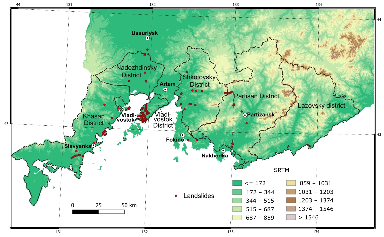
The present study addresses this need by assessing landslide susceptibility in Southern Primorye using a set of natural and environmental predictors, including precipitation, vegetation, lithology, topography, and related territorial characteristics. The study area covers the southern part of Primorsky Krai, including the Khasan, Lazovsky, Partizan, Shkotovsky, and Nadezhdinsky municipal districts, as well as Vladivostok (Figure 1). The landslide occurrence database was compiled from field surveys, scientific and technical publications, reports from local residents, media sources, archived geological and topographic materials, and satellite imagery, including historical imagery available through Google Earth Pro 7.3.7. This approach made it possible to identify additional landslide-like features in Vladivostok and other settlements of Primorye, including Slavyanka, Bezverkhovo, and the Peschany Peninsula. In total, more than 150 landslide occurrences were documented within the study area, most of them located in Vladivostok.

The objectives of this study were to systematize available hydrometeorological, geological, and engineering-geological data for the study area; to identify the main natural factors associated with landslide activation; to train and test a landslide susceptibility model using a GIS-based predictor system and documented landslide occurrences; and to produce a susceptibility map for Southern Primorye. The resulting assessment is intended to support hazard-informed territorial planning, engineering-geological investigations, infrastructure development, and landslide risk reduction in the region. More broadly, the proposed approach may be applicable to other territories with comparable geomorphological, geological, and climatic conditions.

2. Materials and Methods

2.1. Brief Characteristics of the Study Area

The study area covers the southern part of Primorsky Krai (Primorye), including the Khasan, Lazovsky, Partizan, Shkotovsky, and Nadezhdinsky municipal districts, as well as the city of Vladivostok. From a physical-geographical perspective, Primorsky Krai is predominantly a mountainous region located within the mixed forest zone. Its principal relief units are the Sikhote–Alin Range, the East Manchurian Mountains, and the Khanka Plain.

The regional climate is monsoonal and is controlled by seasonal changes in air mass circulation: moist oceanic air dominates in summer, whereas dry and cold continental air prevails in winter. Continentality increases inland with distance from the sea coast.

One of the key factors controlling landslide activation in Primorye is the precipitation regime. It affects rock weathering, soil water saturation, and the predisposition of slope material to displacement. Landslides are generally triggered by prolonged and/or intense rainfall. In terms of precipitation, Primorye belongs to the humid zone. Mean annual precipitation reaches 800–1000 mm in mountainous areas, 600–700 mm in foothill areas, and about 500 mm along the coast of Lake Khanka. Most precipitation falls during the warm season, with a substantial proportion occurring in summer, when torrential rains associated with tropical typhoons and cyclones are common in the region. In the precipitation predictor dataset used in this study, the mean monthly values averaged over a 34-year observation period (1979–2013) for Primorye ranged from 38 mm/month to 100 mm/month, with a mean of 61 mm/month yearly [14].

Geologically, Primorsky Krai is characterized by high structural and lithological heterogeneity. Young geological structures of the Pacific belt with meridional strike intersect with older latitudinal structures extending from the interior of the Asian continent toward the Pacific coast. Within this relatively small territory, sedimentary rocks of various geological ages and diverse magmatic formations are present [18]. The western part of the region belongs to the Khanka Massif, while the eastern part is associated with the folded structures of the Sikhote–Alin system. Neotectonic structures of Mesozoic and Cenozoic age are widely developed [9,10,11,12,13], further contributing to the morphodynamic heterogeneity of the region.

2.2. General Background on Slope Processes in Primorye

Observations of hazardous slope processes in Primorye have been conducted only episodically, mainly after the passage of typhoons and deep cyclones. Available publications and technical reports are rather limited and predominantly descriptive in nature [19]. At the same time, in some sources the southern part of Primorye is classified as a non-debris-flow-prone territory, which does not fully correspond to the slope processes observed in reality.

In the present study, landslide processes are the target of modeling. Debris flows are treated as accompanying hazardous phenomena characteristic of the region but are not included in the target variable of the model. This distinction is necessary for the correct interpretation of the factors controlling the spatial distribution of landslide susceptibility.

The period of probable landslide activation in the study area begins in May and continues until November, with the highest activity generally observed from July to September. This pattern is associated with the passage of deep cyclones and typhoons accompanied by high-intensity rainfall. According to meteorological observations [20], precipitation exceeding 70 mm/day has been recorded repeatedly in the region over the past century. In regional studies, this threshold is regarded as an approximate value beyond which the probability of landslide and debris-flow activation increases substantially [19].

The most significant extreme precipitation events in Primorye are associated with typhoons and tropical cyclones, during which cumulative precipitation in certain areas exceeded 200 mm per event [21]. In recent years, anomalously wet seasons have also been observed. For example, in summer 2023, a significant excess of monthly precipitation norms was recorded across much of the southern coast of the region, and during the influence of Typhoon Khanun in August 2023, extreme precipitation totals were recorded in several areas.

For the study area, two main types of hydrometeorological conditions can be identified as especially favorable for landslide activation:

• Prolonged moderate-intensity rainfall that promotes deep moistening of the slope mass and the accumulation of water in loose deposits.
• Short-duration but intense torrential rainfall associated with tropical cyclones and typhoons, causing rapid overmoistening of soils, surface wash, and slope instability.

2.3. Approaches to Landslide Susceptibility Prediction and Mapping

Each year, geological disasters associated with the movement of earth masses under intense rainfall cause severe social and economic consequences in many countries worldwide. According to [22], 645 fatal landslide events were recorded globally between 1980 and 2018. Over a broader time interval, from 2004 to 2016, the number of recorded cases exceeded 4000, indicating the high relevance of the problem and the growing number of victims [23]. Primorsky Krai, Russia, is also exposed to hazardous landslide processes, many of which are associated with heavy rainfall.

Contemporary climate models indicate a probable increase in the frequency and intensity of extreme precipitation in the future [24]. In particular, models that account for mesoscale moisture convergence as one of the key mechanisms of extreme rainfall generation provide a more accurate description of climate dynamics. The expected intensification of precipitation may therefore lead to an increase in both landslide occurrence and related damage.

The mechanisms of landslide formation vary depending on hydrological conditions, lithological composition, and slope morphology. In one case, when rainfall exceeds the infiltration capacity of the ground, surface runoff develops and may initiate shallow landslides while flowing downslope. In another case, water infiltrates into fractures and pore spaces, increasing hydrostatic pressure, reducing soil strength, and promoting mass displacement along a deeper slip surface. In Primorye, landslides associated with surface runoff are the most typical, although cases related to deeper slip surfaces cannot be excluded.

Two principal approaches to landslide prediction can be distinguished. The first is operational forecasting based on precipitation and other hydrometeorological factors [25,26,27,28]. Such models are generally probabilistic and estimate the likelihood of landslide activation depending on rainfall intensity, duration, and antecedent moisture conditions. Among the methods used, machine learning tools occupy an important place, including logistic regression, which predicts the probability of an event on the basis of external factors.

Logistic regression has been widely applied in operational landslide forecasting [29,30]. For Primorye, this approach was first used to develop a predictive model for the activation of widespread landslide processes based on data from the Vladivostok meteorological station [31]. In that study, a binary classifier distinguishing landslide and non-landslide cases was proposed in the following form:

DR + 0.271 × AR + 0.042 × CP ≥ 122,

(1)

where DR is daily rainfall (mm), AR is antecedent rainfall (mm), and CP is cumulative precipitation since the beginning of the year (mm).

If the sum of the parameters on the left-hand side of Equation (1) exceeds 122, the meteorological conditions are considered sufficient to trigger slope instability in the study area. Model performance was evaluated using historical meteorological records for Vladivostok (World Meteorological Organization Index 31960) covering the period from 1 January 1944 to 1 April 2020, which allowed a statistical relationship to be established between daily rainfall and landslide occurrence [31].

The previously published logistic regression model can therefore be used as a binary classifier of landslide and non-landslide cases based on meteorological data for Primorye. That model showed a balanced accuracy of about 80% [31], indicating strong potential for practical application in early warning systems. By contrast, the current study applies a different susceptibility modeling framework based on OneClassSVM, and its performance is evaluated separately in the Section 3.

The second approach is related to long-term forecasting and aims to identify areas potentially susceptible to landslide activation under the influence of environmental and climatic factors. Landslide susceptibility mapping can be based on both qualitative expert judgment and quantitative techniques using statistical analysis and machine learning algorithms. Susceptibility maps, which characterize the spatial potential for landslide development, are among the most widely used products in this field [32,33,34].

Such maps are commonly generated using models trained on recorded landslide occurrences and the corresponding environmental predictors [35]. Logistic regression remains one of the most widely used and interpretable methods, and probability-based models derived from it have been used, for example, in the production of national landslide hazard maps in several countries [22]. This confirms the high practical relevance of this approach for long-term forecasting and landslide susceptibility mapping.

The general logic of statistical modeling consists of selecting risk-related factors available in a GIS environment and constructing a spatial dataset for model training. The predictors are represented by mapped layers describing terrain properties, climatic conditions, geological structure, vegetation characteristics, and other environmental features. Each georeferenced landslide event is associated with the corresponding set of predictor values at its location.

A binary classifier of this type may be expressed in logistic regression form as follows:

$$Logit\left(P\right)=ln\left({\displaystyle \frac{P\left(Landslide=Yes\right)}{1-P\left(Landslide=Yes\right)}}\right)= {\beta }_0+{\beta }_1\times MMP+{\beta }_2\times Slope+{\beta }_3\times Lithology+{\beta }_4\times LandCover+\cdots$$

(2)

where MMP is long-term mean monthly precipitation, Slope is slope angle, Lithology is the lithological class, LandCover is the vegetation cover type, and (${\beta }_0$, ${\beta }_1$, …, ${\beta }_4$) are model coefficients to be estimated.

A model of this type may also include additional predictors, such as the compound topographic index, runoff characteristics, maximum daily precipitation, and other variables.

Alongside logistic regression, other machine learning algorithms are also widely used for landslide susceptibility mapping. In the present study, a maximum entropy presence-only modeling approach implemented using the OneClassSVM class of the scikit-learn library with a radial basis function kernel was applied. Here, “maximum entropy presence-only modeling approach” refers to the conceptual modeling framework, whereas OneClassSVM denotes its computational implementation. This approach was selected because, for the study area, verified information is primarily available for landslide presence, whereas reliable absence data are limited. In addition, this method allows heterogeneous spatial predictors to be incorporated into landslide susceptibility mapping.

2.4. Main Natural and Climatic Factors Influencing Landslide Activation in Primorye

A landslide inventory database for the study area was compiled through visual analysis of terrain and slope morphology using Google Maps, including its historical imagery function. Cases of rockfalls and debris flows were recorded as accompanying hazardous phenomena characteristic of the region but were not included in the model training dataset. In total, more than 150 confirmed landslide occurrences were identified and used for subsequent analysis of the spatial distribution of the factors controlling landslide susceptibility.

Landslide activation in Primorye is controlled by the combined influence of natural-climatic, geological-geomorphological, and anthropogenic factors. The main natural and climatic factors include the precipitation regime, surface and subsurface runoff conditions, slope morphometry, lithological composition, and vegetation characteristics.

The most significant trigger of landslide activation is prolonged and intense rainfall, which leads to soil saturation, increased pore pressure, and reduced strength of slope materials. Under the monsoonal climate of Primorye, periods associated with the passage of typhoons and deep cyclones accompanied by extreme downpours are especially hazardous. In this context, not only rainfall maxima but also antecedent moisture conditions play a substantial role.

Relief is another important factor, particularly slope steepness, slope form, and slope position within the drainage system. The highest probability of landslide activation is associated with areas where surface and subsurface runoff become concentrated, including lower slope sections and zones of deluvial material accumulation. Slope morphology controls moisture redistribution, washout localization, and the overall stability of the slope mass.

Lithological composition also has a strong influence on landslide development. Slopes composed of loose and weakly consolidated deposits tend to have lower stability and greater susceptibility to displacement under intense wetting. Vegetation characteristics are likewise important, as vegetation affects slope hydrology, infiltration, and the mechanical reinforcement of soils by root systems.

Field observations showed that anthropogenic slope modification may also act as an important local trigger of slope instability in the study area. Slope cutting during road construction, excavation and embankment works, disturbance of natural drainage, and the addition of technogenic materials alter the stress–strain state of the slope mass and create conditions for local slope failure. Particularly high landslide susceptibility is observed in urbanized areas and transport infrastructure zones, where anthropogenic loading is combined with intense surface runoff.

Thus, landslide susceptibility formation in Primorye is determined by the combined interaction of climatic conditions, slope morphology, lithological characteristics, vegetation cover, and anthropogenic impacts. Consideration of these factors as spatial predictors makes it possible to construct a landslide susceptibility mapping model based on a MaxEnt approach.

2.5. Selection and Justification of Predictors

In the present study, factors potentially affecting landslide activation were considered, including the presence of loose and weakly consolidated deposits, vegetation characteristics, slope morphometry, and the precipitation regime. Possible landslide triggers included intense and prolonged rainfall, slope cutting during construction and utility installation, tree removal, slope loading, and other types of anthropogenic disturbance.

Landslide inventories are inherently prone to underreporting and spatial bias, particularly in sparsely populated areas; therefore, the absence of documented occurrences should not be interpreted as an absence of susceptibility. This supports the use of a presence-only modeling approach, although several regional-scale limitations remain. Spatial uncertainties may arise from scale mismatches among predictors and raster resampling during data preparation. Furthermore, due to regional data constraints, direct anthropogenic predictors were not included among the model variables; therefore, human impacts should be interpreted as localized qualitative triggers within the predicted susceptible zones.

A map of long-term mean monthly precipitation was considered as the main climatic predictor. Such a variable has been widely used in landslide susceptibility assessment studies in different regions of the world [22]. In addition to precipitation, the model incorporated morphometric terrain characteristics, lithological features, vegetation cover types, and surface runoff characteristics. A summary of the spatial predictors used in the present study is provided in

Table 1. Predictors used for landslide susceptibility modeling in the study area (coverage: 23,500 km²).

No.	Predictor	Code Name	Description	Source	File Size, MB
1	MMP	prec_south_prim	Mean monthly precipitation (mm/year) for 1979–2013	https://datadryad.org/dataset/doi:10.5061/dryad.kd1d4 (accessed on 7 April 2026)	33
2	Slope	slopes_south_prim	Slope angle, degrees	Computed using RichDEM [36] from the SRTM predictor	33
3	Lithology	litho_south_prim	Lithological class	https://www.dropbox.com/scl/fi/5v00i8op7a9brmn4qeg8b/LiMW_GIS (accessed on 7 April 2026)	33
4	LandCover	globcover_south_prim	Land cover type	https://due.esrin.esa.int/files/Globcover2009_V2.3_Global_.zip (accessed on 7 April 2026)	8.3
5	CTI	cti_south_prim	Compound Topographic Index	Computed from SRTM using the CTI algorithm [37]	33
6	SRTM	srtm_south_prim	Shuttle Radar Topography Mission	SRTM [38,39]	33
7	AF	flow_south_prim	Flow accumulation calculated using the D8 algorithm	https://richdem.readthedocs.io/en/latest/flow_accumulation.html (accessed on 7 April 2026)	33
8	PF	planar_flow_south_prim	Normalized non-channelized surface flow in the range (0, 1)	Computed as the inversely normalized AF value	33

.

2.6. Source Data

2.6.1. Atmospheric Precipitation

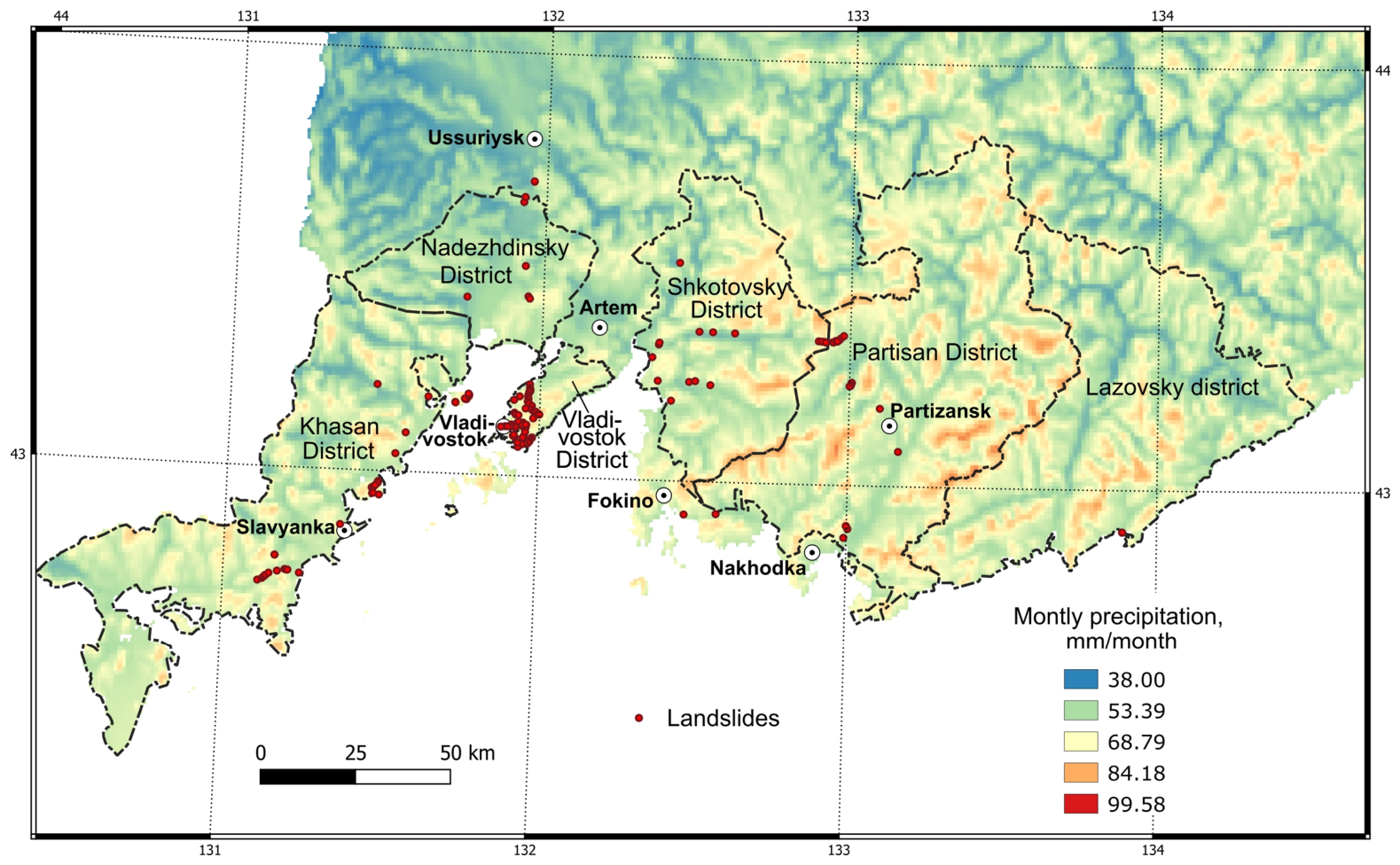
Atmospheric precipitation data were obtained from the CHELSA archive [40], which provides global raster data in GeoTiff format with a spatial resolution of 30 arc-seconds (approximately 1 km). The dataset contains information on monthly precipitation values averaged for the period 1979–2013, derived with consideration of wind direction, slope and valley exposure, ground-based climate observations, and subsequent bias correction [14]. Although the source dataset (Table 1, row 1) provides monthly precipitation values, the model uses mean monthly precipitation (MMP, mm/month), calculated as the average of monthly values over the annual cycle. The precipitation data (Figure 2) were resampled to a common spatial resolution of 79 m/pixel and used for landslide susceptibility model training.

2.6.2. Digital Elevation Model and Slope Map

The SRTM digital elevation model is an important data source for Earth science studies, including hydrological modeling, analysis of erosion and sediment accumulation processes, watershed delineation, and calculation of morphometric terrain parameters. SRTM data were acquired using specialized radar equipment mounted aboard the Endeavour shuttle through interferometric radar measurements [38]. The dataset used in this study represents a global land surface coverage of elevation values with a spatial resolution of 3 arc-seconds, stored in GeoTiff format [39].

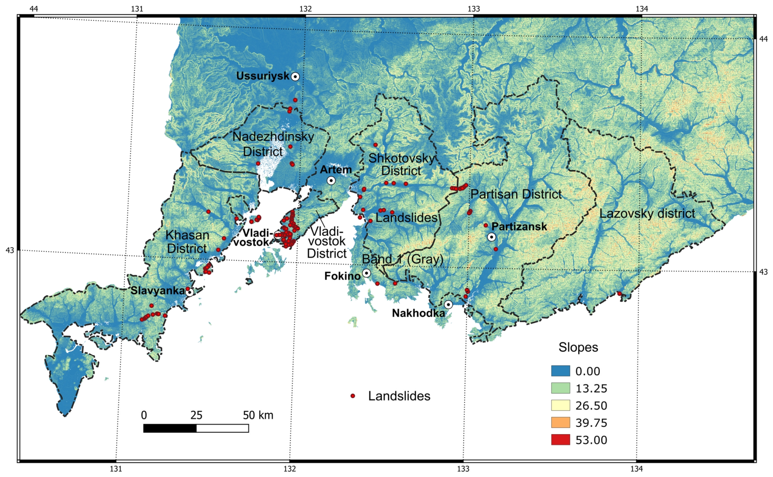
Based on these data, the CTI and Slope predictors were calculated using the developed software prototype (see Table 1). The Slope variable was expressed in degrees and computed using the RichDEM Python module [36]. An overview map of slope steepness for the study area is shown in Figure 3.

2.6.3. Lithological Codes

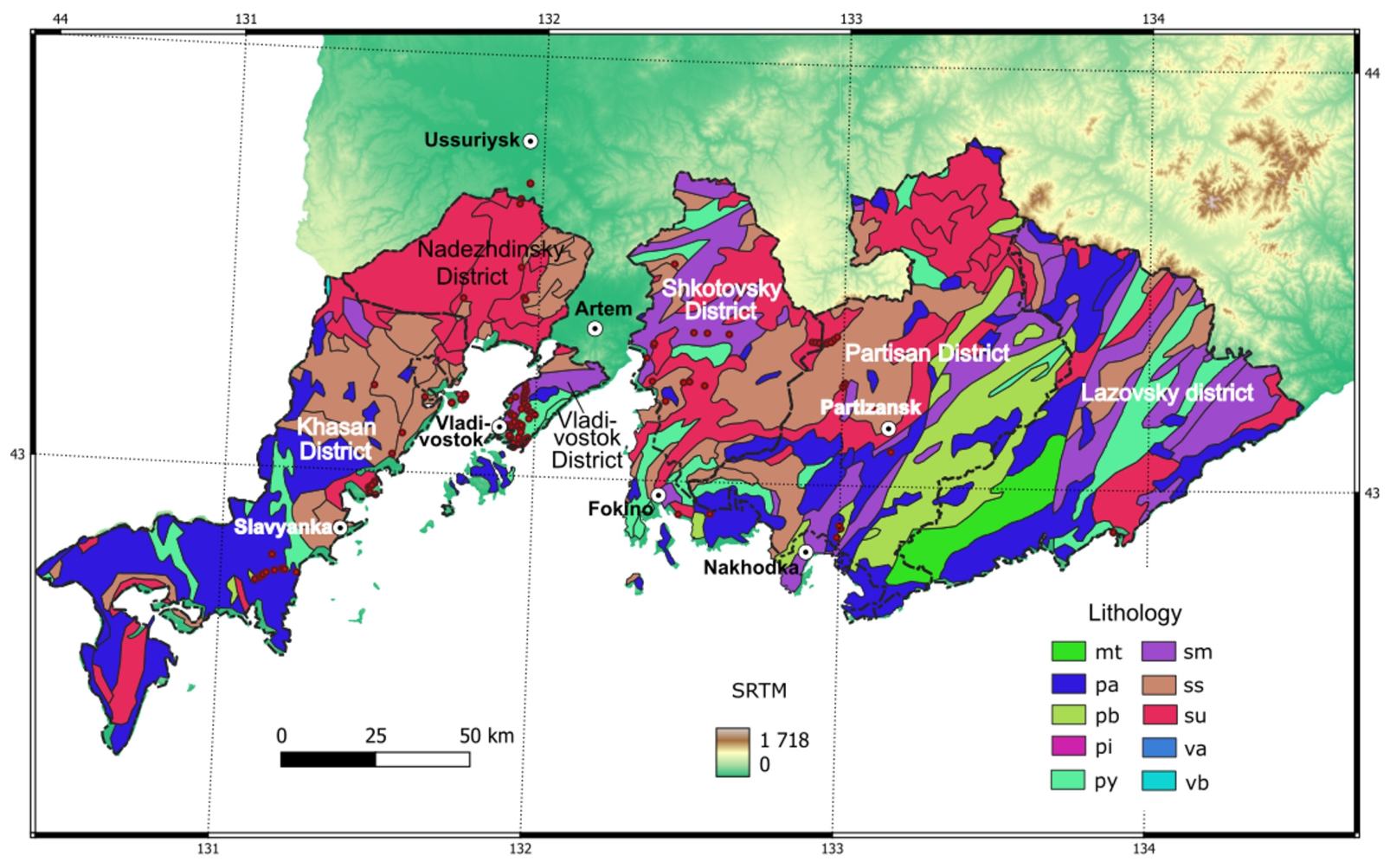
In many cases, recent landslide processes in the region are associated with Neogene and Quaternary formations; therefore, the geological characteristics of the rocks composing the territory must be taken into account in the modeling process. As one of the mapped variables, a high-resolution global lithological map, GLiM, compiled from regional geological maps and lithological information, was used. This dataset enables regional-scale analysis of surface processes at the global level [41]. The spatial distribution of lithological units in the study area and the explanation of lithological class values are shown in Figure 4 and

Table 2. Lithological class codes and corresponding rock density values (g/cm³) after [41,42].

No.	Lithological Code	Rock Class	Density
1	mt	Metamorphic rocks	2.75
2	pa	Acidic magmatic rocks	2.65
3	su	Unconsolidated clastic sedimentary rocks	1.45
4	sm	Mixed sedimentary rocks	2.10
5	ss	Siliciclastic sedimentary rocks	2.30
6	pb	Basic magmatic rocks	2.95
7	py	Pyroclastic volcanic rocks	1.90
8	pi	Intermediate magmatic rocks	2.75
9	vi	Intermediate effusive rocks	2.60
10	vb	Basic effusive rocks	2.85
11	va	Acidic effusive rocks	2.50
12	sc	Carbonate rocks	1.60
13	nd	No data available	1.00
14	wb	* Water bodies	1.00
−9999	else	Errors/Missing values	1.00

* The “wb” class includes not only open water bodies but also water-related landforms with associated unconsolidated sediments.

. Lithological class codes were replaced with corresponding rock density values [42], without interpolation of intermediate values. Unconsolidated deposits generally have lower densities than crystalline rocks (Table 2).

2.6.4. Land Cover Map

Vegetation cover influences soil cohesion, slope resistance to erosion, and the development of landslide processes, while also performing a protective function [15]. The global land cover map used in this study was obtained from the ENVISAT satellite mission using the MERIS spectroradiometer, which records reflected solar radiation in 15 spectral bands within the range 412.5–900 nm [43,44]. Processing of MERIS data to Level 3 made it possible to obtain a validated matrix of land cover classes with a spatial resolution of 300 m/pixel [44]. In the modeling procedure, land-cover class numbers were replaced with relative vegetation cover density values expressed as percentages (

Table 3. Land cover class codes and corresponding vegetation cover percentages (%) after [44].

No.	Value	Vegetation Cover Percentage (%)	Label
1	14	40	Rainfed croplands
2	20	45	Mosaic cropland (50–70%)/vegetation (grassland/shrubland/forest) (20–50%)
3	30	55	Mosaic vegetation (grassland/shrubland/forest) (50–70%)/cropland (20–50%)
4	50	80	Closed (>40%) broadleaved deciduous forest (>5 m)
5	90	30	Open (15–40%) needle-leaved deciduous or evergreen forest (>5 m)
6	100	60	Closed to open (>15%) mixed broadleaved and needleleaved forest (>5 m)
7	110	55	Mosaic forest or shrubland (50–70%)/grassland (20–50%)
8	120	45	Mosaic grassland (50–70%)/forest or shrubland (20–50%)
9	130	40	Closed to open (>15%) (broadleaved or needle-leaved, evergreen or deciduous) shrubland (<5 m)
10	140	30	Closed to open (>15%) herbaceous vegetation (grassland, savannas or lichens/mosses)
11	150	10	Sparse (<15%) vegetation
12	180	50	Closed to open (>15%) grassland or woody vegetation on regularly flooded or waterlogged soil–Fresh, brackish or saline water
13	190	0	Artificial surfaces and associated areas (Urban areas > 50%)
14	200	0	Bare areas
15	210	0	Water bodies

).

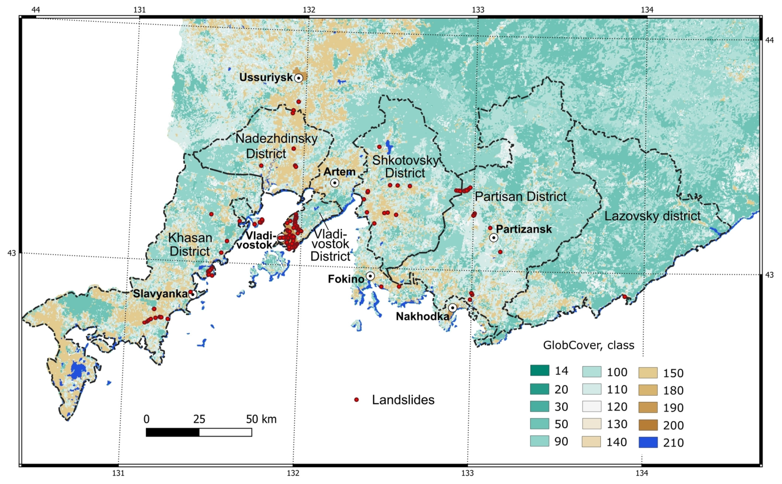
The spatial distribution of land cover classes, as well as water bodies and unvegetated areas, is shown in Figure 5.

Land cover is important for the interpretation of the modeling results because the presence of root systems contributes to the mechanical reinforcement of soils, affects their moisture regime, and reduces the intensity of surface wash. At the same time, changes in vegetation cover, deforestation, and biomass degradation may weaken slope stability. On this basis, the different land cover classes were interpreted as follows:

(14)—rainfed croplands, often characterized by weak root systems of cultivated plants and increased susceptibility to erosion during periods without vegetation cover;

(20)—mosaic croplands combined with woody and shrub vegetation, where plowing increases erosion susceptibility while natural vegetation partly compensates for this effect;

(30)—mosaic agricultural landscapes with a higher proportion of natural vegetation, which generally contributes to greater terrain stability;

(50, 90, 100, 110, 120, 130, 140)—forest, shrubland, and grassland classes, which under natural conditions generally exert a stabilizing effect on slope processes, especially on loose deposits;

(150, 180)—sparse vegetation, providing only weak protection of soils against erosion and slope processes;

(190)—urbanized and built-up areas, where slope stability depends largely on the presence of drainage, erosion-control, and engineering protection measures;

(200)—bare areas, potentially vulnerable to landslide development where loose and weakly consolidated deposits occur;

(210)—shoreline zones of water bodies, where landslide activation may be related to water-level fluctuations and wave action.

2.6.5. Compound Topographic Index

The Compound Topographic Index (CTI) is used to assess the influence of relief on hydrological processes, primarily the ability of different landforms to accumulate and retain water [45]. In geomorphological and engineering-geological studies, CTI is used to identify areas potentially prone to the activation of erosion and slope processes [37]. CTI was calculated according to [37] as follows:

$$CTI=ln\left({\displaystyle \frac{AF}{tan\left(\alpha \right)}}\right),$$

(3)

where AF is the flow accumulation value normalized to the grid-cell size, and α is the slope angle in radians.

All spatial layers were converted to a common analysis grid with a spatial resolution of 79 m/pixel, which ensured their joint use within a unified GIS model. During the preprocessing stage, sets of natural-climatic and morphometric predictors potentially affecting landslide activation were compiled and analyzed. The final model configuration included variables that had clear geomorphological and engineering-geological interpretability and were suitable for spatial association with georeferenced landslide points. A maximum entropy presence-only modeling approach implemented using the OneClassSVM class of the scikit-learn library with a radial basis function kernel was selected because it performs effectively with presence data, does not require reliable absence information, allows heterogeneous spatial predictors to be incorporated, and has been widely applied in spatial susceptibility mapping of natural processes.

3. Results

3.1. Development of the Predictive Model

The development of the landslide prediction model was carried out using elements of the CRISP-DM and Agile methodologies [46,47]. Priority was given to the stepwise development of functional prototypes of a database containing variables that characterize landslide activation factors, as well as a software application for their processing and analysis. The model development process was iterative and involved successive refinement of the data structure, computational procedures, and program code.

The prototype was developed in the browser-based Jupyter Notebook 6.4.12 environment, which is built on the interactive Python 3.9.13 console (IPython). The prototype database was created using a local SQLite server integrated with Python [48,49]. This development environment was chosen because it makes it possible to combine program code, textual comments, Markdown and HTML formatting, and graphical materials within a single workspace.

According to the CRISP-DM methodology [50], the data mining workflow included the following stages: (1) business understanding, (2) data understanding, (3) data preparation, (4) modeling, (5) evaluation, and (6) deployment.

During the business understanding stage, the natural-climatic conditions of Primorye, the geological structure of the area, and its engineering-geological setting were analyzed in order to identify the set of potentially significant landslide-related factors.

During the data understanding stage, a mapping project was created in the QGIS geographic information system, into which raster predictor layers describing the main natural-climatic and morphometric factors of landslide activation were loaded, together with a vector point layer of recorded landslide occurrences. At this stage, the quality of the input data was visually assessed, and their spatial consistency, relevance to the study area, and cartographic projection compatibility were checked.

The data preparation stage included additional topographic calculations, such as deriving the slope map and calculating the Compound Topographic Index from the digital elevation model, as well as resampling all predictor layers to a common spatial resolution and analysis grid. Topographic calculations were performed using the RichDEM module [36], whereas raster harmonization was carried out using the GDAL library [51]. The point layer of recorded landslides was rasterized and stored in GeoTiff format.

During the modeling stage, landslide occurrences identified from published sources and/or remote sensing image interpretation were systematized and mapped. In total, more than 150 reliably documented landslide occurrences were included in the database (see Data Availability section).

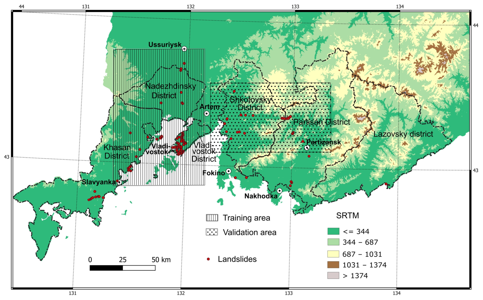
For model training and evaluation, two spatial subsets were selected in southern Primorye. These covered the territory of Vladivostok Urban Okrug, the Nadezhdinsky and Khasan municipal districts, and the Partizan and Shkotovsky municipal districts of Primorsky Krai, respectively (Figure 6).

For spatial landslide susceptibility modeling, a maximum entropy presence-only modeling approach implemented using the OneClassSVM class of the scikit-learn library with a radial basis function kernel was applied. This approach allows the relative degree of spatial susceptibility to landslide activation to be estimated on the basis of mapped predictors and has been widely used for the spatial prediction of natural processes, as well as in geoenvironmental and metallogenic studies [52,53,54]. Unlike models that require reliable information on both presence and absence, the selected approach is focused on modeling spatial susceptibility using landslide presence data, which is particularly important under conditions of incomplete absence information.

Python was used for model implementation. During software development, procedures were created for loading, processing, and spatially associating raster predictor layers with georeferenced landslide points. The model variables consisted of the mapped predictors listed in Table 1.

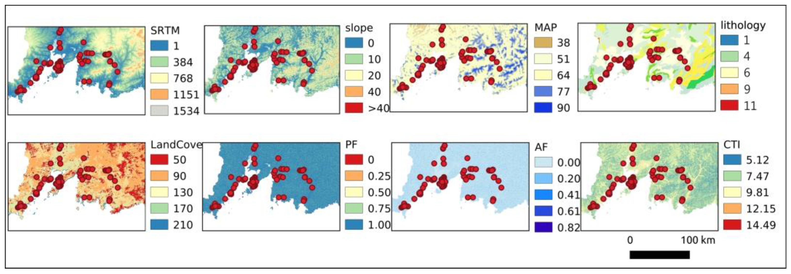
The predictor maps make it possible to visually assess the value ranges and spatial coverage of the input variables (Figure 7). A summary of predictor values inside and outside areas with recorded landslides is provided in

Table 4. Distribution of predictor values in Primorye in relation to recorded landslide occurrences. The category codes and corresponding physical parameter values for Lithology and LandCover are provided in Table 2 and Table 3.

No.	Predictor	Code Name	Description	Values Within Areas with Recorded Landslides			Values Outside Areas with Recorded Landslides
				Min	Mean	Max	Min	Mean	Max
1	MMP	prec_south_prim	Mean monthly precipitation	51.17	59.17	68.25	45.75	62.48	88.75
2	Slope	slopes_south_prim	Slope angle	0	8	27	0	10	51
3	Lithology	litho_south_prim	Lithological class	Categories			Categories
				su, ss, sm, pa			ss, su, sm, py, pa, pb
4	LandCover	globcover_south_prim	Land cover type	Categories			Categories
				90, 110, 50, 150, 120			110, 90, 50, 150, 120, 210, 100, 0, 190
5	CTI	cti_south_prim	Compound Topographic Index	5.85	8.02	13.38	−1.00	8.07	16.14
6	SRTM	srtm_south_prim	Shuttle Radar Topography Mission	5	240	601	1	380	1353
7	AF	flow_south_prim	Flow accumulation	0	0.05	0.44	0	0.046	0.90
8	PF	planar_flow_south_prim	Non-channelized surface flow	0.56	0.95	1	0.1	0.95	1

.

For operation of the software prototype, the data were aggregated into an SQLite database named oegp_dataset_all_prim1.db. A fragment of the Python code used to read raster data in GeoTiff format and extract georeferencing information is provided in Appendix A.1.

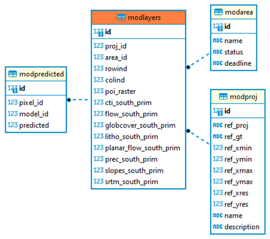
The structure of the database in the form of an Entity–Relationship (ER) diagram is shown in Figure 8. As can be seen from the diagram, the database includes four tables linked through the fields id and prefix_id, where id is the sequential record identifier and prefix_id indicates the table name used to establish the link through the identifier. The database structure was created stepwise using SQL queries provided in Appendix A.2.

Records corresponding to the model training area were then extracted from the developed database. Spatial selection was performed using extent-based queries applied to vector map coverage layers and implemented in the Python prototype.

Before model training, the modlayers table was populated using the GDAL library. Raster datasets were harmonized to a common spatial resolution, and pixel values were extracted according to the row (rowind) and column (colind) indices used in the modlayers table structure.

3.2. Model Training and Testing

The machine learning model was implemented using the OneClassSVM module from the scikit-learn library (Appendix A.3). In the present study, this module was used as a tool for implementing a maximum entropy presence-only modeling approach with a radial basis function kernel [53,54,55]. Here, the term “maximum entropy presence-only modeling approach” refers to the conceptual modeling framework, whereas OneClassSVM denotes the computational implementation used in this study, following the presence-only species distribution modeling example provided in the scikit-learn documentation in the context of MaxEnt-related modeling [55]. This approach was selected because, for the study area, reliable information is available primarily for landslide presence, whereas verified absence data are limited. Despite a strong negative correlation between planar flow and flow accumulation, both variables were retained in the model. The nonlinear OneClassSVM with an RBF kernel can account for predictor interdependence and nonlinear relationships, while the two variables capture complementary hydrological characteristics with opposite effects on landslide susceptibility.

Model development involved constructing a pipeline consisting of two components: a data preprocessing block (preprocessor) and a modeling block (classifier). The preprocessing block was applied to the numerical predictors (cti_south_prim, flow_south_prim, planar_flow_south_prim, prec_south_prim, slopes_south_prim, and srtm_south_prim), which were standardized before model fitting. Before being passed to the model, the categorical variables were converted into physical values (see Table 2 and Table 3 and Appendix A.3 and Appendix A.4) and then standardized. The classifier component consisted of a OneClassSVM model with a radial basis function kernel.

Model hyperparameters were tuned using the GridSearchCV module on the basis of 0.5% of the training area data. During calibration, the values of nu, representing the upper bound on the fraction of training errors and the lower bound on the fraction of support vectors, and gamma, the radial basis function kernel coefficient, were optimized. The selected parameter values were nu = 0.1 and gamma = 0.9.

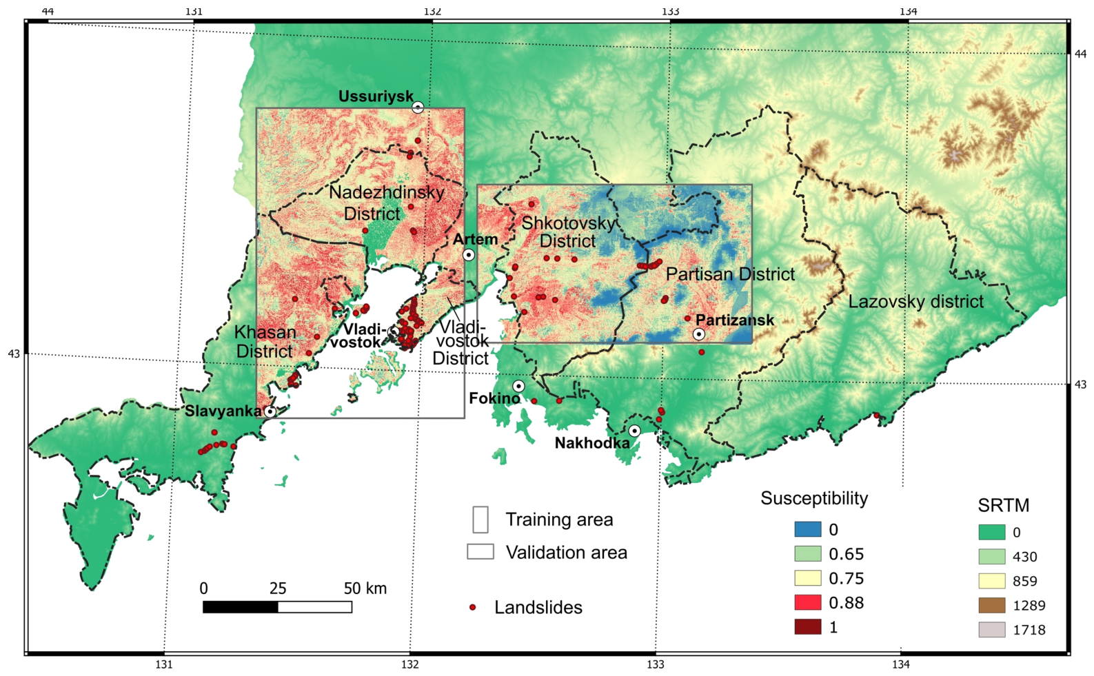
For model development and evaluation, a dual-stage validation strategy was implemented by separating the study region into two distinct geographic zones: a training area and an independent testing area (Figure 9). Within the training area, the data points were partitioned into training and internal validation subsets at an 80:20 ratio, with 80% of the data used for model training and 20% used for internal validation. This partitioning follows common practice in machine learning applications, including Earth science studies [56]. Subsequently, the finalized model was projected onto the independent testing area, where its performance was evaluated against independent landslide occurrence points. Figure 9 shows the modeling results for the training and testing areas; class boundaries were determined using the C-A method [57].

The mapped model output for each raster cell was represented by a normalized decision_function value, interpreted as a landslide susceptibility index. This index reflects the relative proximity of the predictor combination at a given location to the environmental conditions characteristic of areas with recorded landslides.

A fragment of the program code used to extract predictor values from the database for a selected territory, apply the trained model, and write the output values into a table is provided in Appendix A.4.

During the evaluation stage, the trained model was tested primarily in the Shkotovsky and Partizan districts. The model did not use information on known landslide occurrences from this area during training; nevertheless, it successfully delineated their spatial distribution and separated the territory into susceptibility classes (Figure 9).

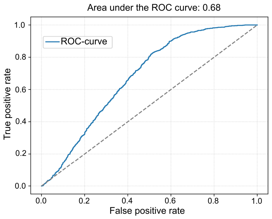
The spatial distribution of the landslide susceptibility index is shown in Figure 9 using a color scale ranging from blue (low susceptibility) to red (high susceptibility). A visual comparison between the documented landslide occurrences in the study area and the model output indicates that the general spatial pattern of landslide-prone areas was captured reasonably well. In addition, the model was quantitatively validated within the independent testing area using the receiver operating characteristic–area under the curve (ROC-AUC) metric (Figure 10).

To address the lack of confirmed absence data inherent in landslide inventories, a balanced pseudo-absence generation strategy was implemented within the testing region. Background samples (pseudo-absences) were randomly extracted from pixels with no recorded landslide occurrences. To ensure a balanced evaluation and reduce classification bias, the number of sampled background points was set equal to the number of documented landslide occurrence points in the testing area, resulting in a 1:1 ratio. Continuous decision function values calculated for both true occurrences and sampled background points were then evaluated across a threshold range from 0 to 1. The false positive rate (FPR) and true positive rate (TPR) were computed based on these balanced classes to construct the ROC curve, yielding an AUC value of 0.68.

The resulting value of ROC-AUC = 0.68 lies at the boundary between moderate and good classification quality [58], which allows the model to be regarded as acceptable for landslide susceptibility mapping. It should be noted, however, that the ROC-AUC value of 0.68 indicates moderate predictive performance. Consequently, the resulting landslide susceptibility map should be interpreted with caution and treated as a baseline exploratory assessment. The uncertainty in the model outputs is primarily attributed to the regional scale of the input data and the limited density of documented landslide occurrences. To reduce these uncertainties and improve model reliability, future iterations of this research should focus on integrating higher-resolution predictor data and expanding the landslide occurrence inventory.

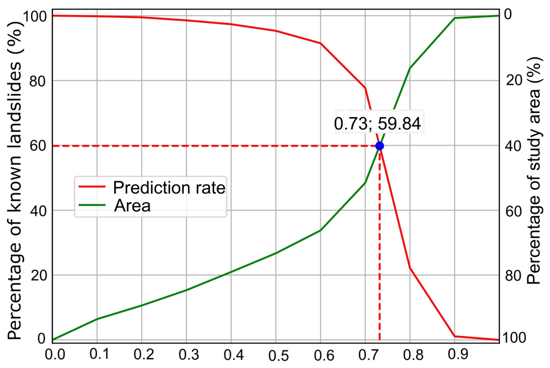
In addition to ROC-AUC, model performance was evaluated using the P–A (probability–area) test [58]. This method allows a threshold susceptibility value to be identified that maximizes the capture of known occurrences within the smallest possible area. According to the results, the intersection point of the probability and prediction curves (0.24; 63.73) indicates that a threshold value of 0.24 delineates 63.73% of known landslide occurrences within 36.27% of the test area (Figure 11). This demonstrates the practical utility of the model and allows the threshold value of 0.24 to be used for distinguishing conditionally safe (<0.73) and conditionally susceptible (≥0.73) areas.

To evaluate predictor contributions, the model-agnostic ‘permutation_importance’ tool from the scikit-learn library was applied. Multiple random shuffles (n_repeats = 10) were performed for each variable, and predictor importance was estimated from the mean decrease in the ROC-AUC score. This procedure helped reduce the influence of random fluctuations and provided a more stable assessment of predictor contributions for the implemented nonlinear model. Using the approach proposed by [59], predictor importance for distinguishing between conditionally safe and conditionally susceptible areas was also evaluated (

Table 5. Predictor importance in the classification of conditionally safe and conditionally susceptible areas.

No.	Predictor	Importance in Classification
1	MMP	0.0057
2	Slope	0.0290
3	Lithology	0.0039
4	Landcover	0.0401
5	CTI	0.0453
6	AF	0.0640
7	PF	0.0640
8	SRTM	0.1097

).

As shown in Table 5, the most influential predictors in the model are absolute elevation (SRTM), planar flow (PF), accumulated flow (AF), compound topographic index (CTI), and landcover type (Landcover). The remaining predictors play a subordinate role.

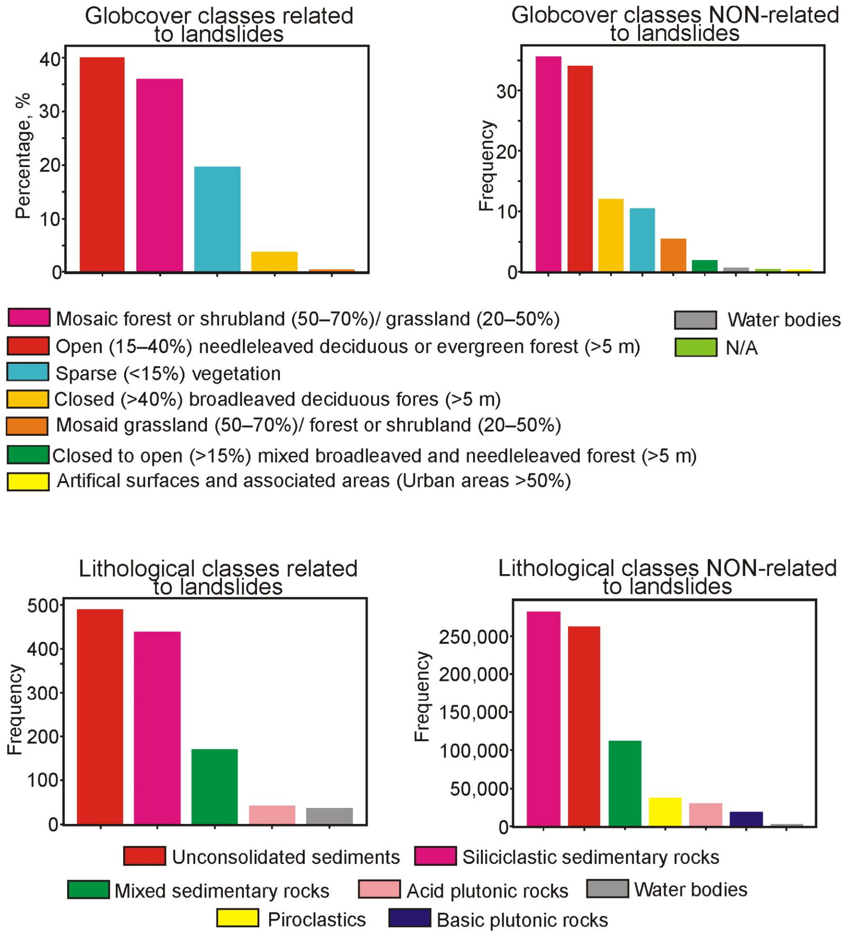
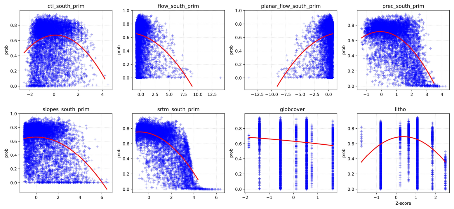
The next stage of model evaluation involved clarifying the role of individual predictors using partial dependence curves for the numerical variables (Figure 12) and histograms of categorical variable distributions (Figure 13).

Figure 12 displays the partial dependence curves, illustrating the nonlinear responses of individual continuous predictors to landslide susceptibility. The curves indicate that areas with elevated landslide susceptibility are associated with gentle slopes located in the middle and lower parts of river valleys, where the contribution of non-channelized surface flow (planar_flow) increases and the influence of channelized runoff (flow_accumulation) decreases. Complementarily, Figure 13 shows the distribution of landslide occurrences across environmental classes using frequency histograms.

The data indicate that, within the identified susceptible zones, loose unconsolidated materials and sparse woody vegetation or open woodland are more common than other lithological and land-cover classes. These combined results are consistent with general concepts of slope instability and suggest that hydrological factors, geological conditions, and vegetation characteristics jointly influence the spatial distribution of landslides in the study area.

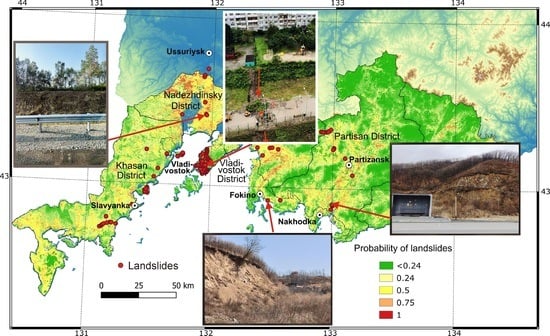
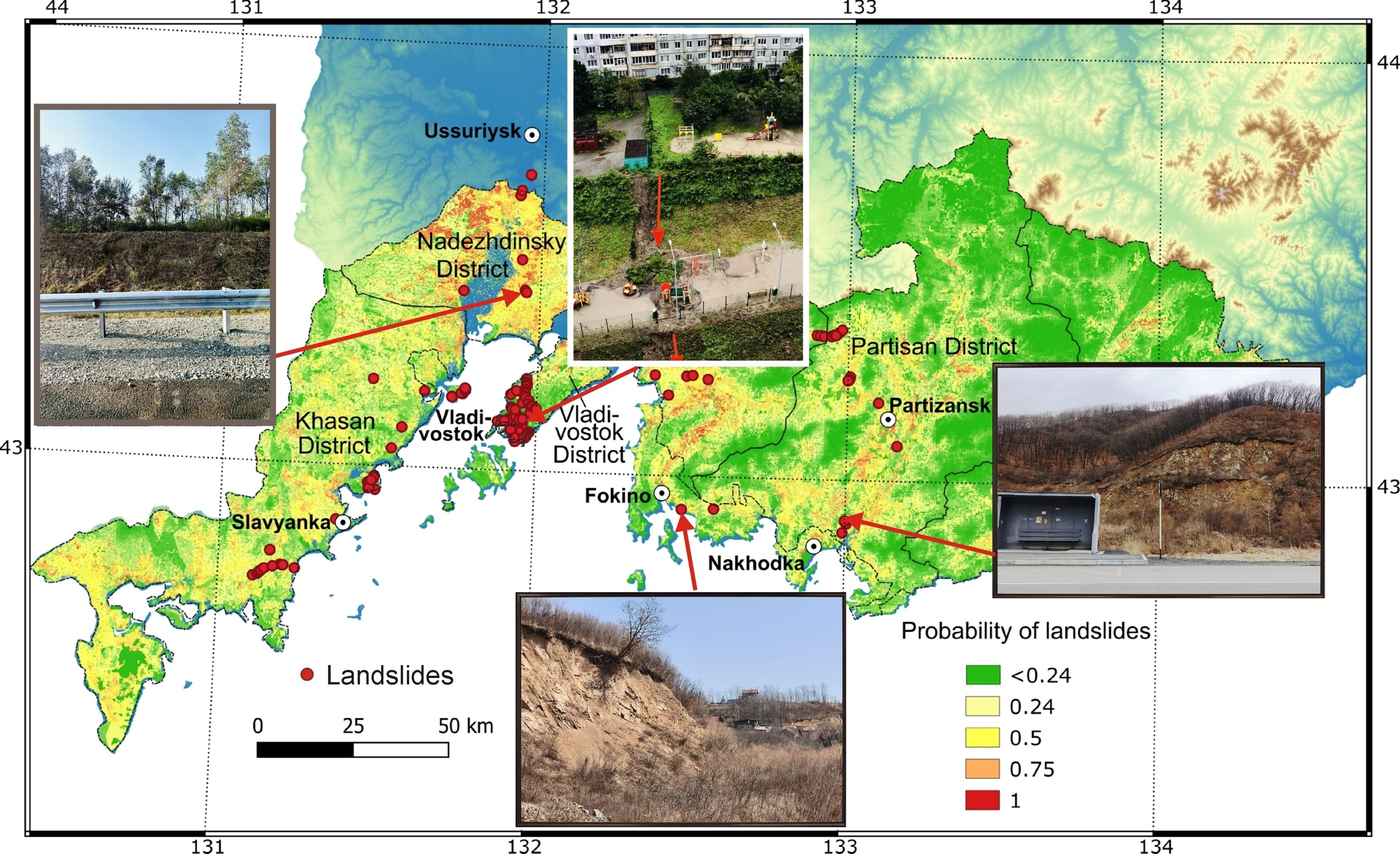
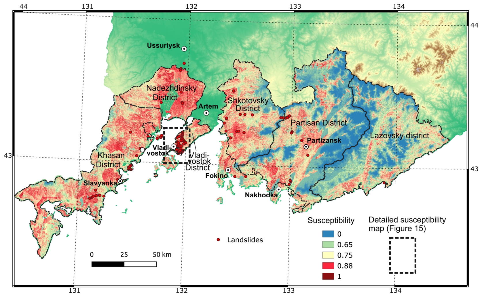
Based on the modeling results, a landslide susceptibility map for southern Primorye was produced (Figure 14). The map reflects the spatial distribution of areas with different degrees of susceptibility to landslide activation and can be used as a supporting tool in engineering-geological investigations, settlement planning, transport and energy infrastructure development, and the placement of other socially and economically important facilities.

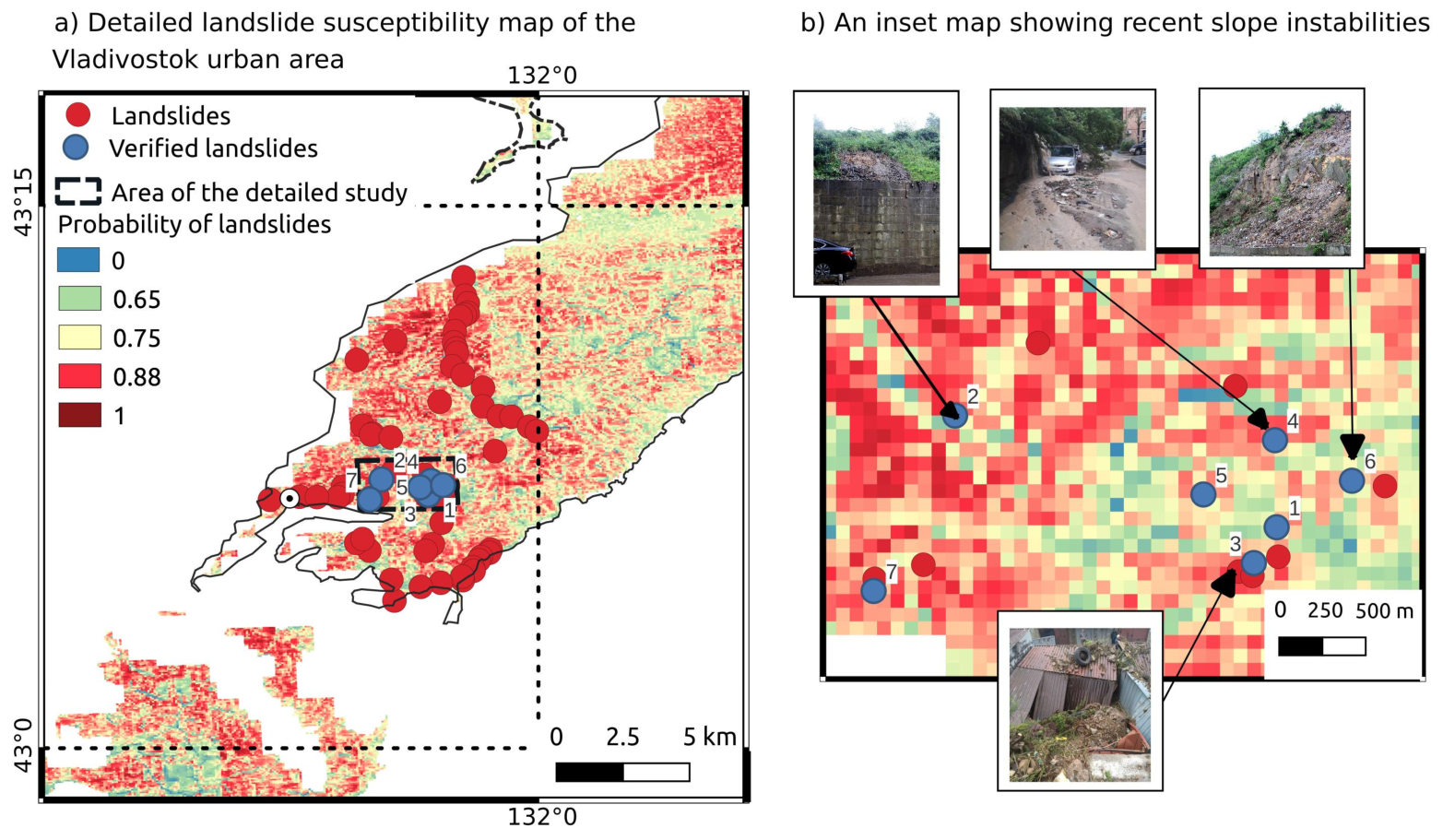
We validated the landslide susceptibility map against documented historical landslide events within the Vladivostok urban area, which were not used for model training and were reported by local media sources (

Table 6. Documented landslide occurrences within high-susceptibility zones in the Vladivostok urban area, corresponding to the inset map in Figure 15b.

ID	Location	Date	Media Reports
1	Vladivostok, Ladygina st.	August 2019	https://www.newsvl.ru/vlad/2024/08/24/225977/ (accessed on 26 June 2026)
2	Vladivostok, Tobolskaya st.	August 2019	https://vladnews.ru/2019-08-27/157813/vladivostoke_mashiny (accessed on 26 June 2026)
3	Vladivostok, 5-Terrasnaya st.	August 2019	https://www.newsvl.ru/vlad/2019/08/28/183365/ (accessed on 26 June 2026)
4	Vladivostok, Adm. Kuznetsova st.	August 2019	https://www.nn.ru/text/world/2024/09/28/74147645/ (accessed on 26 June 2026)
5	Vladivostok, Adm. Kuznetsova st.	July 2019	https://www.newsvl.ru/vlad/2024/08/24/225977/ (accessed on 26 June 2026)
6	Vladivostok, Ladygina st.	May 2019	https://www.newsvl.ru/vlad/2019/05/28/181002/ (accessed on 26 June 2026)
7	Vladivostok, Slavyanskaya st.	August 2024	https://primpress.ru/article/115274 (accessed on 26 June 2026)

). Figure 15 presents a detailed landslide susceptibility map of the Vladivostok urban area (a), accompanied by an inset map showing recent slope instabilities (b). The historically documented landslide occurrence points shown in Figure 15 generally coincide with zones classified as having high landslide susceptibility, particularly where the modeled susceptibility index exceeds 0.88. The inset map (b) illustrates the spatial distribution of recent slope movements recorded in the late 2010s, which were compiled and cross-checked using local media reports.

Thus, the modeling results made it possible to refine the understanding of the spatial distribution of landslide-prone areas in Southern Primorye and to identify potential directions for the practical application of the proposed approach in sustainable territorial planning, land-use regulation, infrastructure development, and natural hazard risk management. The resulting susceptibility map can serve as a spatial decision-support tool for identifying areas where detailed engineering-geological investigations, monitoring, or preventive measures should be prioritized.

4. Discussion

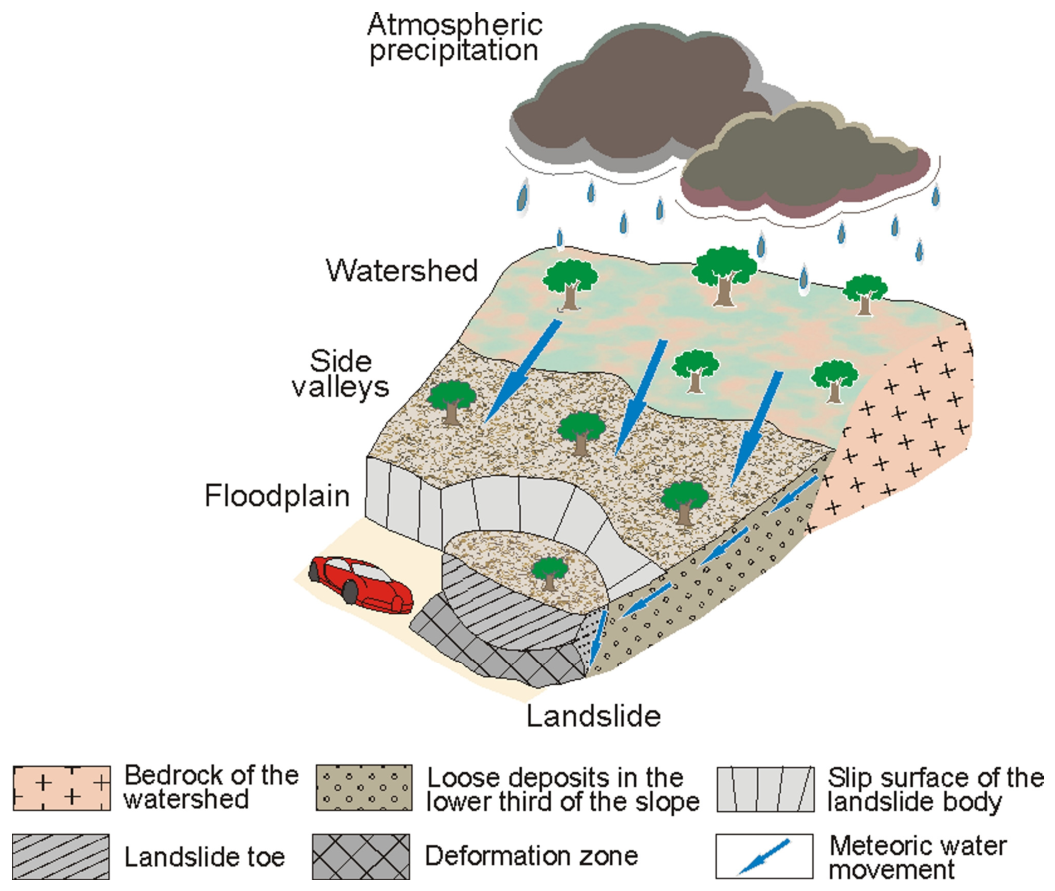
Considering the identified predictor importance, the highest landslide susceptibility within the study region is associated with lower slope sections and coastal landforms composed of loose unconsolidated deposits and partially covered by sparse woodland. Surface and subsurface runoff from watershed areas, which receive a substantial proportion of regional precipitation, plays an important role in creating conditions favorable for slope instability. The interpretive conceptual diagram presented in Figure 16 illustrates these conditions, including meteoric water movement from watershed areas, the presence of loose deposits under sparse woody vegetation, and anthropogenic slope cutting by road excavations, which may contribute to landslide activation.

While direct anthropogenic parameters (e.g., distance to roads or excavation intensity) were not explicitly included as predictors in the model, field observations confirmed that localized slope cutting can contribute to terrain destabilization. Consequently, the model-derived susceptibility maps delineate areas with elevated landslide susceptibility, within which human activity may act as an important external trigger. These field-verified anthropogenic impacts are therefore discussed as supplementary qualitative context for the quantitative model outputs.

The present study proposes an approach to landslide susceptibility prediction and mapping based on the integration of remote sensing data, GIS-derived morphometric parameters, geological information, vegetation characteristics, and precipitation data. For spatial modeling, a presence-only approach implemented using the OneClassSVM class of the scikit-learn library with a radial basis function kernel was applied. Its application in Southern Primorye made it possible to delineate regional landslide susceptibility zones and capture the main spatial patterns of landslide-prone areas despite inventory constraints. Given the model’s ability to identify broad susceptibility patterns, the resulting map should be considered a regional baseline framework, within which field-verified anthropogenic activities may act as important localized triggers.

The results indicate that land cover characteristics, terrain position, atmospheric precipitation, and lithological properties exert the strongest influence on the final model. Together, these factors reflect both natural controls on slope instability and the degree of anthropogenic transformation of the territory. Importantly, elevated susceptibility to landslide activation was identified not only on steep slopes but also on gentle slopes located in the lower parts of slope systems, where loose material accumulates, surface and subsurface runoff becomes concentrated, and the natural slope profile may be disturbed by human activity. This combination of factors is consistent with the observed conditions of landslide development in the region.

The proposed approach extends beyond conventional geological mapping by considering landslide susceptibility as a spatial basis for hazard-informed territorial planning, engineering assessment, and infrastructure risk management. The resulting map can be used in engineering-geological investigations, in the selection of sites and corridors for transport and energy infrastructure, and in the assessment of land-use suitability in areas with complex terrain. In this respect, susceptibility mapping can contribute to more sustainable territorial development by helping to avoid or minimize the use of areas where slope instability may create unacceptable risks.

From the perspective of hazards and sustainability, the practical value of the proposed framework lies in its ability to integrate heterogeneous geospatial data into a unified natural hazard assessment system. This is particularly important for coastal and mountainous environments, where infrastructure development is often accompanied by substantial anthropogenic impacts on relief, drainage conditions, and slope stability. The results therefore provide a basis for improving land-use regulation, prioritizing detailed engineering-geological surveys, planning mitigation measures, and reducing exposure of infrastructure and settlements to landslide hazards.

The study also has several limitations that should be considered when interpreting the results. The landslide inventory is based on a combination of field data, literature sources, local reports, media information, and satellite image interpretation, which may lead to spatial incompleteness and uneven representation of landslide occurrences. In addition, the susceptibility model reflects the influence of the selected predictors at the available spatial resolution and does not account for short-term triggering conditions such as individual rainfall events, rapid snowmelt, or local engineering disturbances. Therefore, the resulting map should be interpreted as a regional-scale susceptibility assessment rather than a deterministic prediction of landslide occurrence.

As one of the first regional-scale landslide susceptibility assessments for Primorye, this study has limited direct local benchmarks for comparison. Nevertheless, the identified predictor patterns and moderate model performance (AUC = 0.68) are generally consistent with previous landslide susceptibility studies conducted in comparable geomorphological settings and provide a basis for future, more localized research. Future research should focus on improving the landslide inventory, increasing the spatial and temporal resolution of input data, and incorporating dynamic triggering factors, particularly precipitation intensity and duration. The integration of susceptibility maps with monitoring data and scenario-based hazard assessment could further enhance their practical value for risk reduction and sustainable territorial planning in Primorsky Krai. Such developments would support more effective infrastructure management, preventive planning, and long-term reduction in landslide-related losses in the region.

5. Conclusions

This study developed an approach to landslide susceptibility mapping in Southern Primorye based on the integration of heterogeneous geospatial data, including remote sensing products, morphometric terrain parameters, geological characteristics, vegetation information, and atmospheric precipitation data. For spatial modeling, a presence-only approach implemented using the OneClassSVM class of the scikit-learn library with a radial basis function kernel was applied. The results showed that the highest landslide susceptibility is associated with lower slope sections and coastal landforms composed of loose unconsolidated deposits and partially covered by sparse woodland. The main factors contributing to slope instability include atmospheric moisture conditions, surface and subsurface runoff, lithological properties, and anthropogenic slope cutting related to road infrastructure.

The practical significance of the study lies in the potential use of the resulting regional-scale landslide susceptibility map as a baseline layer for sustainable territorial planning and broad-scale infrastructure zoning. This map serves as an exploratory tool for identifying broad susceptibility patterns and delineating priority areas for subsequent detailed monitoring. Overall, the study demonstrates the potential of integrating machine learning, GIS, and remote sensing for regional susceptibility mapping, emphasizing that the output represents a broad-scale framework rather than a site-specific slope stability assessment. Future research will focus on refining the landslide inventory, incorporating higher-resolution spatial data, and moving toward dynamic hazard modeling.

References

1. Osipov, V.I. Megacities under the threat of natural disasters. Her. Russ. Acad. Sci. 1996, 66, 771–782. [Google Scholar]
2. Ragozin, A.L. General provisions for assessment and management of natural risks. Environ. Geosci. 1999, 5, 417–429. [Google Scholar]
3. Perez, L.P.; Martins, J.R.S. Vulnerability to landslides in the city of Sao Paulo. J. Civ. Eng. Archit. 2016, 10, 1160–1167. [Google Scholar] [CrossRef]
4. Haque, U.; Blum Ph da Silva, P.F.; Andersen, P.; Pilz, J.; Chalov, S.R.; Malet, J.-P.; Auflič, M.J.; Andres, N.; Poyiadji, E.; Lamas, P.C.; et al. Fatal landslides in Europe. Landslides 2016, 13, 1545–1554. [Google Scholar] [CrossRef]
5. Cogan, J.; Gratchev, I.; Wang, G. Rainfall-induced shallow landslides caused by ex-Tropical Cyclone Debbie, 31st March 2017. Landslides 2018, 15, 1215–1221. [Google Scholar] [CrossRef]
6. Mateos, R.M.; López-Vinielles, J.; Poyiadji, E.; Tsagkas, D.; Sheehy, M.; Hadjicharalambous, K.; Liscák, P.; Podolski, L.; Laskowicz, I.; Iadanza, C.; et al. Integration of landslide hazard into urban planning across Europe. Landsc. Urban Plan. 2020, 196, 103740. [Google Scholar] [CrossRef]
7. Macias, L.; Quiñonez-Macías, M.; Toulkeridis, T.; Pastor, N.J. Characterization and geophysical evaluation of the recent 2023 Alausí landslide in the northern Andes of Ecuador. Landslides 2024, 21, 529–540. [Google Scholar] [CrossRef]
8. Gao, H.; Xu, C.; Xie, C.; Ma, J.; Xiao, Z. Landslides triggered by the July 2023 extreme rainstorm in the Haihe River Basin, China. Landslides 2024, 21, 2885–2890. [Google Scholar] [CrossRef]
9. Goryachev, N.A.; Pirajno, F. Gold deposits and gold metallogeny of Far East Russia. Ore Geol. Rev. 2014, 59, 123–151. [Google Scholar] [CrossRef]
10. Kruk, N.N.; Simanenko, V.P.; Gvozdev, V.I.; Golozubov, V.V.; Kovach, V.P.; Serov, P.I.; Kholodov, V.V. Geochemical characteristics and sources of the melts of the Early Cretaceous granitoids in the Samarga terrain (Sikhote-Alin). Russ. Geol. Geophys. 2014, 55, 276–302. [Google Scholar] [CrossRef]
11. Khanchuk, A.I.; Kemkin, I.V.; Kruk, N.N. The Sikhote-Alin orogenic belt, Russian South East: Terranes and the formation of continental lithosphere based on geological and isotopic data. J. Asian Earth Sci. 2016, 120, 117–138. [Google Scholar] [CrossRef]
12. Soloviev, S.G.; Kryazhev, S.G.; Avilova, O.V.; Andreev, A.V.; Girfanov, M.M.; Starostin, I.A. The Lazurnoe deposit in the Central Sikhote-Alin, Eastern Russia: Combined shoshonite-related porphyry Cu-Au-Mo and reduced intrusion-related Au mineralization in a post-subduction setting. Ore Geol. Rev. 2019, 112, 103063. [Google Scholar] [CrossRef]
13. Shevyrev, S.; Carranza, E.J.M. Modelling of geodynamic regimes of precious metal-bearing porphyry deposits: Lazurnoe deposit (Sikhote–Alin Belt, Far East) case study. Geol. J. 2020, 55, 8309–8328. [Google Scholar] [CrossRef]
14. Karger, D.N.; Conrad, O.; Böhner, J.; Kawoh, T.; Kreft, H.; Soria-Auza, R.W.; Zimmermann, N.E.; Linder, H.P.; Kessler, M. Data from: Climatologies at High Resolution for the Earth’s Land Surface Areas. Sci. Data 2017, 4, 170122. [Google Scholar] [CrossRef] [PubMed]
15. Li, Y.; Duan, W. Decoding vegetation’s role in landslide susceptibility mapping: An integrated review of techniques and future directions. Biogeotechnics 2024, 2, 10005. [Google Scholar] [CrossRef]
16. Miao, Z.; Cheng, Z.; Xiong, Y.; Wu, L.; Zhang, H.; Li, Z.B.; Peng, Z.; Liu, D. Landslide susceptibility mapping under cropland expansion: Considering root cohesion variability and land use effects on saturated hydraulic conductivity. Geomat. Nat. Hazards Risk 2025, 16, 2569797. [Google Scholar] [CrossRef]
17. Steger, S.; Moreno, M.; Crespi, A.; Gariano, S.L.; Brunetti, M.T.; Melillo, M.; Peruccacci, S.; Marra, F.; de Vugt, L.; Zieher, T.; et al. Adopting the margin of stability for space–time landslide prediction—A data-driven approach for generating spatial dynamic thresholds. Geosci. Front. 2024, 15, 101822. [Google Scholar] [CrossRef]
18. Khanchuk, A.I.; Ratkin, V.V.; Ryazantseva, M.D.; Golozubov, V.V.; Gonokhova, N.G. Geology and Mineral Deposits of Primorsky Krai (Territory); Dalnauka: Vladivostok, Russia, 1995; pp. 1–81. [Google Scholar]
19. Stepnova, Y.; Gensiorovskiy, Y.; Lobkina, V.; Muzychenko, L.; Muzychenko, A.; Orekhov, A.; Stepnov, A.; Konovalov, A. Exogenous geodynamic processes activation in the south of Primorsky Krai in August 27–28, 2019. Vestn. Far East Branch Russ. Acad. Sci. 2021, 2, 42–54. [Google Scholar] [CrossRef]
20. Weather and Climate. Available online: http://www.pogodaiklimat.ru (accessed on 26 February 2026).
21. History of Typhoons and Powerful Cyclones in the Far East. Available online: https://maglipogoda.ru/istoriya-tayfunov-i-moshhnykh-ciklonov-na/ (accessed on 26 February 2026).
22. Lin, Q.; Lima, P.; Steger, S.; Glade, T.; Jiang, T.; Zhang, J.; Liu, T.; Wang, Y. National-scale data-driven rainfall induced landslide susceptibility mapping for China by accounting for incomplete landslide data. Geosci. Front. 2021, 12, 101248. [Google Scholar] [CrossRef]
23. Froude, M.J.; Petley, D. Global fatal landslide occurrence from 2004 to 2016. Nat. Hazards Earth Syst. Sci. 2018, 18, 2161–2181. [Google Scholar] [CrossRef]
24. Chang, P.; Fu, D.; Liu, X.; Castruccio, F.S.; Prein, A.F.; Danabasoglu, G.; Wang, X.; Bacmeister, J.; Zhang, Q.; Rosenbloom, N.; et al. Future extreme precipitation amplified by intensified mesoscale moisture convergence. Nat. Geosci. 2026, 19, 33–41. [Google Scholar] [CrossRef]
25. Liu, G.; Liu, D.; Li, T.; Wang, F.; Zou, T. Joint probability prediction model of rainfall triggered landslides and debris flows. Open J. Geol. 2012, 2, 103–110. [Google Scholar] [CrossRef]
26. Auflič, M.J.; Šinigoj, J.; Krivic, M.; Podboj, M.; Peternel, T.; Komac, M. Landslide prediction System for rainfall induced landslides in Slovenia (Masprem). Geologija 2016, 59, 259–271. [Google Scholar] [CrossRef]
27. Kuradusenge, M. Predictive Modelling and Alert System for Rainfall Induced Landslides. Ph.D. Thesis, University of Rwanda College of Science and Technology, Kigali, Rwanda, 28 June 2022. [Google Scholar]
28. Kang, J.; Wan, B.; Gao, Z.; Zhou, S.; Chen, H.; Shen, H. Research on machine learning forecasting and early warning model for rainfall-induced landslides in Yunnan province. Sci. Rep. 2024, 14, 14049. [Google Scholar] [CrossRef] [PubMed]
29. Hong, M.; Kim, J.; Jeong, S. Rainfall intensity-duration thresholds for landslide prediction in South Korea by considering the effects of antecedent rainfall. Landslides 2018, 15, 523–534. [Google Scholar] [CrossRef]
30. Kuradusenge, M.; Kumaran, S.; Zennaro, M. Rainfall-induced landslide prediction using machine learning models: The case of Ngororero district, Rwanda. Int. J. Environ. Res. Public Health 2020, 17, 4147. [Google Scholar] [CrossRef] [PubMed]
31. Stepnova, Y.A.; Stepnov, A.A.; Konovalov, A.V.; Gensiorovskiy, Y.V.; Lobkina, V.A.; Muzychenko, L.E.; Muzychenko, A.A.; Orekhov, A.A. Predictive model of rainfall-induced landslides in high-density urban areas of the South Primorsky Region (Russia). Pure Appl. Geophys. 2022, 179, 4013–4024. [Google Scholar] [CrossRef]
32. Oliveira, S.C.; Zêzere, J.L.; Garcia, R.A.C.; Pereira, S.; Vaz, T.; Melo, R. Landslide susceptibility assessment using different rainfall event-based landslide inventories: Advantages and limitations. Nat. Hazards 2024, 120, 9361–9399. [Google Scholar] [CrossRef]
33. Danese, M.; Lazzari, M. A kernel density estimation approach for landslide susceptibility assessment. In Proceedings of the International Conference on “Mountain Risks: Bringing Science to Society”, Florence, Italy, 24–26 November 2010; pp. 101–107. [Google Scholar]
34. Wang, C.; Zhou, J.; Wang, Z.; Yang, Y.; Lu, J.; Kang, D.; Wang, S.; Zhang, H. Assessment of landslide susceptibility in watersheds during extreme rainfall using a complex network of slope units. Sci. Rep. 2025, 15, 5194. [Google Scholar] [CrossRef] [PubMed]
35. Chiang, J.L.; Kuo, C.M.; Fazeldehkordi, L. Using deep learning to formulate the landslide rainfall threshold of the potential large-scale landslide. Water 2022, 14, 3320. [Google Scholar] [CrossRef]
36. RichDEM—High Performace Terrain Analysis. Available online: https://richdem.readthedocs.io/en/latest/ (accessed on 16 March 2026).
37. Verdin, K. Final Report: High Resolution Topographic Analysis for GMAO’s Catchment LSM, 2013: Available at Global Modeling and Assimilation Office, Code 610.1, NASA/Goddard Space Flight Center, Greenbelt, MD 201771. Available online: https://gmao.gsfc.nasa.gov/gmaoftp/sarith/ROUTING_MODEL/docs/SRTM_TopoData_CompletionReport_Verdin2013.pdf (accessed on 10 April 2026).
38. SRTM Shuttle Radar Topography Mission, NASA Earth Observing System. Available online: https://eospso.nasa.gov/missions/shuttle-radar-topography-mission (accessed on 12 March 2026).
39. SRTM 90 m DEM Digital Elevation Database. Available online: https://srtm.csi.cgiar.org/ (accessed on 12 March 2026).
40. CHELSA—Climatologies at High Resolution for the Earth Land Surface Areas. Version 1.2. Available online: https://data.europa.eu/data/datasets/0101a156-14d9-41cc-b49a-9424e8b047d1?locale=en (accessed on 10 March 2026).
41. Hartmann, J.; Moosdorf, N. The new global lithological map database GLiM: A representation of rock properties at the Earth surface. Geochem. Geophys. Geosystems 2012, 13, Q12004. [Google Scholar] [CrossRef]
42. Turcotte, D.L.; Schubert, G. Geodynamics, 3rd ed.; Cambridge University Press: Cambridge, UK, 2014; pp. 1–636. [Google Scholar] [CrossRef]
43. Bicheron, P.; Defourny, P.; Brockmann, C.; Schouten, L.; Vancutsem, C.; Huc, M.; Bontemps, S.; Leroy, M.; Achard, F.; Herold, M.; et al. GLOBCOVER: Products Description and Validation Report, 2008. Available online: https://due.esrin.esa.int/files/GLOBCOVER_Products_Description_Validation_Report_I2.1.1.pdf (accessed on 8 April 2026).
44. GlobCover: Global Land Cover Map, 2009. Available online: https://developers.google.com/earth-engine/datasets/catalog/ESA_GLOBCOVER_L4_200901_200912_V2_3?hl=ru (accessed on 7 April 2026).
45. Buttrick, S.; Popper, K.; McRae, B.; Unnasch, B.; Schindel, M.; Jones, A.; Platt, J. Conserving Nature’s Stage: Identifying Resilient Terrestrial Landscapes in the Pacific Northwest; Technical Report; The Nature Conservancy: Arlington, VA, USA, 2015. [Google Scholar] [CrossRef]
46. Karpov, D.V. Agile methodology of software development. Vestn. Lobachevsky Univ. Nizhni Novgorod 2011, 3, 227–230. [Google Scholar]
47. Gubin, E.I. Big data preparation technique for predictive analysis. Nauka I Bizn. Puti Razvit. (Sci. Bus. Paths Dev.) 2020, 3, 33–35. [Google Scholar]
48. Jupyter Notebook. Available online: https://jupyter.org/ (accessed on 16 March 2026).
49. SQLite Homepage. Available online: https://sqlite.org/ (accessed on 16 March 2026).
50. What is CRISP DM? Available online: https://www.datascience-pm.com/crisp-dm-2/ (accessed on 19 March 2026).
51. GDAL Documentation. Available online: https://gdal.org/en/stable/ (accessed on 17 March 2026).
52. Phillips, S.J.; Anderson, R.P.; Schapire, R.E. Maximum entropy modeling of species geographic distributions. Ecol. Model. 2006, 190, 231–259. [Google Scholar] [CrossRef]
53. Shevyrev, S.; Carranza, E.J.M. Application of Maximum Entropy for mineral prospectivity mapping in heavily vegetated areas of Greater Kurile chain with Landsat 8 data. Ore Geol. Rev. 2022, 142, 104758. [Google Scholar] [CrossRef]
54. Shevyrev, S.L.; Boriskina, N.G.; Ivin, V.V. Principal component analysis for geochemical data analysis and chemical elements associations of prospective Kolumbe area (Kema terrain, Sikhote-Alin folded belt). Russ. J. Earth Sci. 2024, 2, 1–9. [Google Scholar] [CrossRef]
55. Species Distribution Modeling. Available online: https://scikit-learn.org/stable/auto_examples/applications/plot_species_distribution_modeling.html (accessed on 29 May 2026).
56. Merriam, D.F.; Drew, L.J.; Schuenemeyer, J.H. Zipf’s Law: A Viable Geological Paradigm? Nat. Resour. Res. 2004, 13, 265–271. [Google Scholar] [CrossRef]
57. Yousefi, M.; Carranza, E.J.M. Prediction area (P-A) plot and C-A fractal analysis to classify and maps for mineral prospectivity modelling. Comput. Geosci. 2015, 79, 69–81. [Google Scholar] [CrossRef]
58. Pourghasemi, H.R.; Kerle, N. Random forests and evidential belief function-based landslide susceptibility assessment in Western Mazandaran Province. Iran. Environ. Earth Sci. 2016, 75, 185. [Google Scholar] [CrossRef]
59. Alghofaili, Y. Interpretable K-Means: Clusters Feature Importances–Towards Data Science. Available online: https://towardsdatascience.com/interpretable-k-means-clusters-feature-importances-7e516eeb8d3c (accessed on 13 March 2026).
60. Shevyrev, S.L. SergeiShevyrev, Landslides. Available online: https://github.com/SergeiShevyrev/SergeiShevyrev/blob/main/landslides (accessed on 1 June 2026).
Figure 1. Location of the study area in Southern Primorye and SRTM-based digital elevation model showing documented landslide occurrences.
Sustainability 18 06797 g001
Figure 2. Overview map of mean monthly precipitation for the period 1979–2013 in the study area, after [40].
Sustainability 18 06797 g002
Figure 3. Overview map of slope steepness in the study area.
Sustainability 18 06797 g003
Figure 4. Lithological map of the study area. The lithological codes are explained in Table 2.
Sustainability 18 06797 g004
Figure 5. Land cover map of the study area. The land cover class codes are detailed in Table 3.
Sustainability 18 06797 g005
Figure 6. Areas selected for model training and testing in Primorye.
Sustainability 18 06797 g006
Figure 7. Visualization of raster predictor layers. The variable name is shown on the right-hand side of each image above the legend.
Sustainability 18 06797 g007
Figure 8. Structure of the study database shown as an ER diagram.
Sustainability 18 06797 g008
Figure 9. Model validation in the test and training areas shown over a shaded digital elevation model.
Sustainability 18 06797 g009
Figure 10. ROC-AUC metric for the model test area.
Sustainability 18 06797 g010
Figure 11. P–A balance curves.
Sustainability 18 06797 g011
Figure 12. Partial dependence plots for numerical predictors.
Sustainability 18 06797 g012
Figure 13. Histograms of land cover and lithology categories for the test area.
Sustainability 18 06797 g013
Figure 14. Landslide susceptibility map of southern Primorye.
Sustainability 18 06797 g014
Figure 15. Detailed landslide susceptibility map of the Vladivostok urban area (a). An inset map showing recent slope instabilities (b). Blue numbered points correspond to the landslide records listed in Table 6. Original photographs were taken by A. Orekhov (FEGI FEB RAS).
Sustainability 18 06797 g015
Figure 16. Conceptual model of conditions associated with elevated landslide susceptibility in southern Primorye.
Sustainability 18 06797 g016