PFAD: Parameter-Efficient Framework for Cross-Domain Anomaly Detection for Sustainable Manufacturing

Abstract

Deploying visual anomaly detection in industrial production requires retraining models for each product domain, leading to substantial costs in data collection, computational resources, and energy consumption that scale poorly across diverse manufacturing environments. This paper proposes PFAD, a parameter-efficient framework for cross-domain anomaly detection without retraining, enabling the direct deployment of a source model trained on a benchmark dataset to unseen industrial settings in a zero-shot manner. PFAD leverages a frozen vision transformer backbone and introduces Soft Anomaly-Aware Feature Selection (Soft AFS), which assigns continuous weights to feature channels based on anomaly discriminability, preserving information while enhancing cross-domain generalization without relying on synthetic anomalies or target-domain data. Extensive experiments on both public benchmarks and real-world industrial datasets demonstrate that PFAD achieves strong cross-domain performance, including an image-level AUROC of 0.945 for semiconductor PCB inspection using only a public dataset for training. Furthermore, PFAD supports an optional one-shot inference extension, where a single normal reference image improves detection performance in scenarios with large domain gaps (up to $+10.4$ pp), most effectively when zero-shot transfer leaves meaningful headroom. These results demonstrate that PFAD provides a practical and scalable solution for industrial anomaly detection by eliminating repeated retraining cycles and reducing associated computational and energy overhead, while maintaining high performance across heterogeneous domains.

1. Introduction

The rapid advancement of Industry 4.0 and smart manufacturing has elevated intelligent quality inspection to a critical function in modern production systems [1,2,3]. Automated visual anomaly detection (AD) is now widely deployed across industries such as semiconductor manufacturing, pharmaceuticals, and precision manufacturing, where manual inspection cannot meet the increasing demands for throughput, consistency, and reliability [4,5,6,7]. In semiconductor fabrication, for example, each new process node or product generation introduces inspection requirements that existing models cannot satisfy—driving repeated model development cycles that delay yield ramp and increase time-to-market. In pharmaceutical manufacturing, regulatory mandates for 100% visual inspection, combined with frequent batch and formulation changes, mean that inspection systems must be rapidly deployable across diverse product configurations without lengthy model development pipelines.

Despite significant progress in benchmark performance, most existing AD systems remain inherently domain-dependent: models trained on one product category or inspection environment typically fail to generalize to others. As a result, deploying AD in real-world factories requires repetition of the full pipeline of data collection, annotation, model training, and validation for every new product line. This per-domain retraining paradigm introduces substantial operational costs. As product portfolios grow, cumulative GPU computation, energy consumption, and engineering labor scale proportionally—directly undermining the resource efficiency and sustainability goals of modern manufacturing [8].

The limitations of this paradigm can be summarized in three dimensions. First, data collection and curation must be repeated for each product variant [9], requiring significant engineering effort to gather representative normal samples and validate defect patterns. Second, computational overhead accumulates across retraining cycles: repeated GPU-intensive training for each product variant generates energy consumption that, when multiplied across a multi-line facility, represents a non-trivial environmental burden inconsistent with the sustainability commitments increasingly adopted across manufacturing sectors. Third, models trained in one domain often exhibit severe performance degradation when transferred to another [10,11], reflecting their reliance on domain-specific visual features such as texture, color distribution, and imaging conditions. Together, these three dimensions constitute a sustainability barrier that scales adversely with product portfolio diversity. These challenges motivate a fundamental research question: To what extent can an anomaly detection model trained on a source dataset be directly deployed to unseen industrial domains without requiring any target-domain data or retraining?

Recent research has explored zero-shot AD approaches, particularly those based on vision–language models (VLMs) [12,13,14,15], which leverage textual prompts to define normality and abnormality. While promising, these methods introduce new complexities, including dependence on language encoders, sensitivity to prompt design, and the use of additional adaptation modules. In industrial inspection settings—where anomalies are often subtle, domain-specific, and purely visual—such dependencies can limit practicality and require expertise that may not be available on the factory floor. VLM-based methods may struggle in underrepresented industrial domains where visual–textual co-occurrence during pretraining is limited [15].

An alternative direction is represented by vision-only approaches based on frozen foundation models. Notably, UniADet [16] demonstrates that strong zero-shot and few-shot anomaly detection performance can be achieved without language encoders by learning lightweight decoupled direction vectors ($W_{\mathrm{cls}}$, $W_{\mathrm{seg}}$) on top of frozen vision transformers (e.g., DINOv2 [17], DINOv3 [18]). However, this approach treats all feature channels equally, implicitly assuming that each channel contributes uniformly across domains. We hypothesize that this assumption is problematic in cross-domain settings: some channels encode domain-specific information (e.g., texture and color) that can act as noise during cross-domain transfer, thereby degrading the learned direction vectors on unseen target domains. In a deployment context, this means that a source model may degrade unpredictably when transferred to a production line with different surface characteristics or imaging conditions, even when the inspection task is structurally similar. This hypothesis motivates our graded channel-weighting design (Section 3.3).

Feature selection methods provide a complementary solution by identifying channels most relevant for anomaly detection. RealNet [19] introduced Anomaly-aware Feature Selection (AFS), a self-supervised method that evaluates each channel’s anomaly discriminative capability and selects the top-$m_k$ channels via hard thresholding. While effective within a single domain, such hard selection strategies discard a large portion of the feature space, causing information loss. This limitation is particularly critical in cross-domain scenarios: channels discarded based on the source domain may be precisely those needed to detect defects in an unseen target domain.

To address these limitations, we propose PFAD, a framework for retraining-free cross-domain deployment that combines the strengths of both approaches with two key improvements:

1.

Soft AFS: We propose a soft, information-preserving alternative to RealNet’s hard channel selection [19], replacing binary top-k masks with a softmax-based weighting mechanism (w $=\mathrm{softmax}(-\mathrm{MSE}/{\tau }_{\mathrm{afs}})\times d$) that retains all channels while calibrating anomaly-relevant ones. This preserves information from channels that may be less important in the source domain but critical in unseen target domains. The absolute performance gain over uniform channel weighting is modest (at most $+0.11$ pp image-level AUROC on public benchmark pairs; Section 4.4.1); its primary value lies in statistical stability and calibrated selectivity across diverse domain-transfer scenarios.

2.

Real defect-based calibration: Instead of relying on synthetic anomalies (e.g., SDAS in RealNet), we calibrate channel weights using source-domain data, eliminating the distribution gap between synthetic and real anomalies.

In this work, “retraining-free” refers specifically to target-domain deployment: PFAD is trained once on a selected public source dataset and then transferred to unseen target lines without any target-side data collection or optimization. This design directly reduces the cumulative computational, energy, and engineering overhead associated with deploying inspection across multiple product lines, supporting the resource-efficiency goals of sustainable manufacturing.

Our contributions are as follows:

1.

We introduce Soft AFS, a method for channel-level, anomaly-aware weighting that improves cross-domain transferability while preserving feature information. This approach enables new product lines to be commissioned by training the model once on an appropriate public source dataset and deploying the resulting source model without target-domain retraining.

2.

We propose calibrating AFS weights using source-domain data, eliminating dependence on synthetic anomaly generation pipelines and leveraging existing inspection records.

3.

We demonstrate that training only 0.02 M parameters on a frozen backbone reduces per-domain setup to approximately 18 minutes on a single GPU, enabling integration into production-line quality management systems without dedicated AI infrastructure.

4.

We validate PFAD on both public benchmarks (MVTec AD, VisA, BTAD, KolektorSDD) and real industrial datasets (semiconductor PCB inspection and pharmaceutical packaging), demonstrating that the same PFAD architecture transfers across heterogeneous industrial target domains—semiconductors and pharmaceuticals—without any per-domain retraining.

5.

We provide an optional single-reference one-shot pathway that can further improve detection at inference time when zero-shot performance has room for improvement—e.g., Mono → RGB sensor transfer ($+4.8$ pp) or large domain-gap scenarios such as Pharma (up to $+10.4$ pp)—without requiring any additional training.

2. Related Work

2.1. Unsupervised Anomaly Detection

Unsupervised AD methods train exclusively on normal images and can be categorized into three main categories. Embedding-based methods such as PatchCore [10] leverage pre-trained features to separate anomalies in feature space. Discrimination-based methods reframe AD as supervised learning via synthetic pseudo-anomalies. Reconstruction-based methods detect anomalies based on reconstruction errors, assuming anomalous regions cannot be faithfully reconstructed. DINOmaly [11] (CVPR 2025) builds minimal-adaptation heads on frozen DINOv2 features for multi-class unsupervised AD, achieving strong within-domain performance; however, it requires independent training on each target dataset and does not support cross-domain zero-shot transfer. RealNet [19] combines hard AFS with synthetic anomaly generation (SDAS) for single-domain training. Recent studies have further extended unsupervised AD to unified frameworks: Jézéquel et al. [20] introduced a multi-scale contrasted memory approach that supports both zero-shot and few-shot settings within a single model. These methods are inherently constrained to seen classes and require retraining for each new domain.

2.2. Zero-Shot and Few-Shot Anomaly Detection

Zero-shot AD has gained traction through VLMs such as CLIP [21]. WinCLIP [12] introduces two-class textual prompts with multi-scale patch windows. AnomalyCLIP [13] learns class-agnostic prompt embeddings. AdaCLIP [14] and Bayes-PFL [22] integrate visual knowledge into prompt spaces. AdaptCLIP [15] proposes lightweight adapters with alternating learning strategies that partially address domain representation gaps in industrial settings. InCtrl [23] holistically integrates multi-level features for few-shot classification. Despite progress, VLM-based methods anchor features to CLIP’s visual-textual co-occurrence space and typically require per-domain prompt engineering or adapter retraining, with fewer than 1 million adapter/prompt parameters per domain; they may struggle in niche industrial domains under-represented in pre-training. Few-shot learning has also been applied to industrial fault diagnosis with limited labeled data [24], highlighting the broader demand for sample-efficient adaptation methods in manufacturing. Recent studies have also addressed domain gaps between pre-trained representations and target inspection scenarios in few-shot settings [25], and cross-domain zero-shot transfer has been explored via logit-space consistency constraints [26].

UniADet [16] demonstrates that language encoders are unnecessary by directly learning decoupled direction vectors ($\sim 0.02$ million parameters) on frozen vision foundation models (DINOv2 [17], DINOv3 [18]), achieving strong cross-domain zero-shot results without language supervision. Our work extends this architecture with soft, calibrated channel weighting (Soft AFS) to improve robustness to domain-specific channel activation shifts that raw direction vectors cannot anticipate.

2.3. Feature Selection for Anomaly Detection

RealNet [19] introduced AFS, which evaluates each channel’s ability to discriminate between normal and anomalous regions via MSE against ground-truth masks and performs hard top-k selection. While effective within a single domain, this approach suffers from information loss and domain-specific bias in cross-domain settings. Our Soft AFS addresses these limitations by assigning continuous weights to all channels, providing a more flexible mechanism for cross-domain transfer.

Despite strong benchmark results, these methods have been primarily validated on curated academic datasets; their applicability to real industrial inspection lines under strict operational constraints—no downtime for retraining, heterogeneous sensors, diverse product variants—remains largely unexplored [1,9].

Table 1. Comparison of PFAD with related zero-/few-shot anomaly detection methods. PF = Prompt-free; ZS = Zero-Shot (target-domain); FS = Few-Shot; XDom = Cross-domain transfer without target retraining; Train. Params = learnable parameters during source-domain training (frozen backbone excluded throughout). ✓ = supported; ✗ = not supported.

Method	Backbone	PF	ZS	FS	XDom	Train. Params
WinCLIP [12]	CLIP ViT	✗	✓	✓	Limited	0 (infer. only)
AnomalyCLIP [13]	CLIP ViT	✗	✓	✗	Limited	<0.1M (prompts)
AdaCLIP [14]	CLIP ViT	✗	✓	✓	Limited	<1M (prompts)
AdaptCLIP [15]	CLIP ViT	✗	✓	✓	✓	<1M (adapters)
DINOmaly [11]	DINOv2 ViT	✓	✗	✗	✗	per-dataset
UniADet [16]	DINOv3 ViT	✓	✓	✓	✓	∼$0.02$ M
PFAD (ours)	DINOv3 ViT	✓	✓	✓	✓	0.02 M

summarizes the positioning of PFAD relative to existing methods.

3. Proposed Method

3.1. Overview

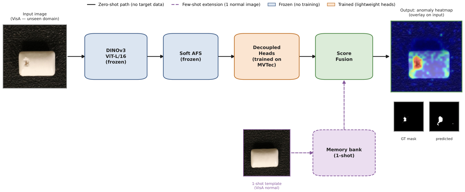
The PFAD pipeline consists of four components: (A) a frozen DINOv3 backbone for multi-scale feature extraction; (B) Soft AFS for channel weighting via one-time calibration; (C) decoupled classification and segmentation heads; and (D) score fusion for final predictions. An optional (E) memory bank supports the few-shot extension (Section 3.6). Figure 1 illustrates the overall architecture.

3.2. DINOv3 Backbone

We employ DINOv3 ViT-L/16 [18] as a frozen feature extractor (300 M parameters, no gradient computation). Given an input image $X\in {\mathbb{R}}^{3\times 512\times 512}$, features are extracted from five intermediate Transformer blocks $\{11,14,17,20,23\}$ (0-indexed), yielding per-layer outputs:

$$x_q^l\in {\mathbb{R}}^d,F_q^l\in {\mathbb{R}}^{N\times d},$$

(1)

where $x_q^l$ is the global CLS token, $F_q^l$ are local patch tokens, $d=1024$, and $N=32\times 32=1024$ patches.

3.3. Soft Anomaly-Aware Feature Selection

3.3.1. Motivation

Not all $d=1024$ channels are equally useful for anomaly detection; treating them with uniform weights [19] is a simplification that can degrade cross-domain transfer. Some channels encode domain-specific information (e.g., texture patterns, color distributions) that does not generalize across domains. RealNet’s hard AFS selects $m_k\ll d$ channels per layer, but this discards potentially useful information for unseen target domains.

3.3.2. Calibration Procedure

Soft AFS is a one-time calibration performed prior to training, consisting of three phases.

Phase 1 (Normal Reference): Normal test images from the source domain are passed through the backbone, and the mean patch feature per layer is computed:

$${\mu }_{\mathrm{normal}}^l={\displaystyle \frac{1}{|{\mathcal{D}}_{\mathrm{good}}|}}\sum _{X\in {\mathcal{D}}_{\mathrm{good}}}{F}^l\left(X\right).$$

(2)

Phase 2 (Channel-wise MSE Scoring): For each defect image with ground-truth mask M, the squared feature difference from the normal reference is computed per channel i:

$${\mathcal{L}}_{\mathrm{AFS}}^l\left(i\right)={\displaystyle \frac{1}{|{\mathcal{D}}_{\mathrm{defect}}|}}\sum _{X\in {\mathcal{D}}_{\mathrm{defect}}}{∥\mathcal{F}\left({\left[F_i^l\left(X\right)-{\mu }_{\mathrm{normal},i}^l\right]}^2\right)-M∥}_2^2,$$

(3)

where $\mathcal{F}(·)$ performs min-max normalization and resolution alignment to the mask.

Phase 3 (Soft Weighting): Instead of hard top-k selection, we compute continuous channel weights:

$${\mathbf{w}}^l=softmax\left({\displaystyle \frac{-{\mathrm{MSE}}^l}{{\tau }_{\mathrm{afs}}}}\right)\times d,$$

(4)

where ${\tau }_{\mathrm{afs}}=0.1$ is the temperature parameter controlling weight sharpness, and scaling by $d=1024$ ensures $\mathbb{E}\left[w_i\right]\approx 1$ to preserve feature magnitude.

3.3.3. Application

During both training and inference, features are reweighted element-wise as follows:

$${\tilde{x}}_q^l=x_q^l\odot {\mathbf{w}}^l,{\tilde{F}}_q^l=F_q^l\odot {\mathbf{w}}^l.$$

(5)

Algorithm 1 summarizes the full calibration procedure.

Source-domain data requirements. Soft AFS calibration (Algorithm 1) and direction-vector training require: (i) normal images from the source domain, and (ii) anomaly images with pixel-level GT masks. This is a one-time source-domain setup ($\approx 18$ min on RTX A6000). Target-domain deployment requires no additional data, labels, or retraining (zero-shot). For the optional one-shot extension (Section 3.6), a single normal reference image from the target domain is sufficient.

Algorithm 1 Soft AFS Calibration

Require:  Normal images ${\mathcal{I}}_n$, anomaly images ${\mathcal{I}}_a$ with GT masks $\mathcal{M}$, temperature ${\tau }_{\mathrm{afs}}$, frozen backbone f Ensure:  Per-layer channel weights ${\left\{w^l\right\}}_{l\in \mathcal{L}}$ 1: ${\mu }_c^l\leftarrow {\displaystyle \frac{1}{|{\mathcal{I}}_n|·N}}{\sum }_{i,p}{f}_c^l\left(x_{i,p}\right)$    ▹ mean normal patch feature per channel/layer 2: for $(I_a,M)\in ({\mathcal{I}}_a,\mathcal{M})$ do 3:     for $l\in \mathcal{L}$ do 4:         ${\mathrm{mse}}_c^l+={\mathrm{mean}}_{\mathrm{anomaly}\mathrm{patches}}\left[{(F_c^l\left(I_a\right)-{\mu }_c^l)}^2\right]$ 5:     end for 6: end for 7: Average ${\mathrm{mse}}^l$ across all anomaly images 8: $w^l\leftarrow softmax(-{\mathrm{mse}}^l/{\tau }_{\mathrm{afs}})\times d$

3.4. Decoupled Classification and Segmentation Heads

Following UniADet [16], we decouple image-level anomaly classification and pixel-level anomaly segmentation with independent learnable direction vectors per layer l:

$$W_{\mathrm{cls}}^l\in {\mathbb{R}}^{2\times d},W_{\mathrm{seg}}^l\in {\mathbb{R}}^{2\times d}.$$

(6)

The anomaly scores are computed via cosine similarity with temperature scaling:

$${\widehat{y}}^l=softmax\left({\displaystyle \frac{\langle W_{\mathrm{cls}}^l,{\tilde{x}}_q^l\rangle }{\tau }}\right),{\widehat{Y}}^l=softmax\left({\displaystyle \frac{\langle W_{\mathrm{seg}}^l,{\tilde{F}}_q^l\rangle }{\tau }}\right),$$

(7)

where $\tau =0.1$. Multi-scale predictions are aggregated by averaging across the five layers.

3.5. Score Fusion

The final image-level anomaly score fuses the classification score with the maximum segmentation score:

$${\widehat{y}}_f=(1-{\lambda }_p)·{\widehat{y}}_{\mathrm{cls}}+{\lambda }_p·\underset{i,j}{max}\left({\widehat{Y}}_{\mathrm{seg}}\right),$$

(8)

where ${\lambda }_p=0.5$. The pixel-level anomaly map ${\widehat{Y}}_{\mathrm{seg}}$ is upsampled to the original resolution using bilinear interpolation (mode="bilinear", align_corners=False, scale factor = patch size = 16) for evaluation.

3.6. Few-Shot Extension via Score-Level Fusion

While the zero-shot pipeline requires no target-domain data, PFAD can be extended to a few-shot setting when a small number of normal reference images from the target domain are available. Following the few-shot inference strategy of UniADet [16], we construct a memory bank from the support image(s) and fuse the resulting scores with the zero-shot predictions at the score level, requiring no additional training.

3.6.1. Memory Bank Construction

Given K normal support images from the target domain ($K=1$ in our experiments), we extract patch-level features from the frozen backbone and build a per-layer memory bank:

$${\mathcal{M}}^l=\left\{{\tilde{F}}_s^l\left(j\right)|j=1,\dots ,N,s=1,\dots ,K\right\}\in {\mathbb{R}}^{(K·N)\times d},$$

(9)

where each patch feature is ${\mathcal{\ell }}_2$-normalized and AFS-reweighted.

3.6.2. Few-Shot Anomaly Scoring

For each query patch token ${\tilde{F}}_q^l\left(j\right)$, the few-shot anomaly score is computed as the complement of the maximum cosine similarity to the memory bank:

$$s_{\mathrm{few}}^l\left(j\right)=1-\underset{m\in {\mathcal{M}}^l}{max}cos\left({\tilde{F}}_q^l\left(j\right),m\right).$$

(10)

The per-layer scores are averaged across layers to obtain the final few-shot segmentation map $S_{\mathrm{few}}\in {\mathbb{R}}^N$.

3.6.3. Score-Level Fusion

The few-shot segmentation scores are fused with the zero-shot scores via a weighted combination:

$$\begin{array}{c}{S}_{\mathrm{fused}}=(1-{\lambda }_f)·{\widehat{Y}}_{\mathrm{seg}}+{\lambda }_f·S_{\mathrm{few}},\end{array}$$

(11)

$$\begin{array}{c}{\widehat{y}}_f=(1-{\lambda }_p)·{\widehat{y}}_{\mathrm{cls}}+{\lambda }_p·max\left(S_{\mathrm{fused}}\right),\end{array}$$

(12)

where ${\lambda }_f$ controls the balance between zero-shot and few-shot segmentation signals. We set ${\lambda }_f=0.5$ throughout all few-shot experiments, following UniADet [16], which treats the two signals equally. ${\lambda }_f$ is applied at few-shot inference only and is independent of training.

We evaluate this optional extension in two practical settings where target-side normal references are available: (1) cross-modality paired inference on the SemiCond dataset, where each test image has a spatially aligned normal counterpart from a different sensor, and (2) patch-level inference on the Pharma dataset, where high-resolution images are divided into a $2\times 2$ grid with position-specific memory banks to capture spatially variant anomaly patterns. As shown in Section 4.3.1 and Section 4.3.2, its benefit depends on the zero-shot headroom and on the compatibility of the reference image with the target feature distribution.

3.7. Training

3.7.1. Training Protocol

Following UniADet [16], we adopt the same cross-domain evaluation protocol: PFAD is trained using data from a source dataset and evaluated on entirely distinct target datasets in a zero-shot manner. Since the source and target domains share no overlapping categories or images, evaluation integrity on the target is fully preserved. The combined loss is defined as follows:

$$\mathcal{L}={\mathcal{L}}_{\mathrm{CE}}({\widehat{y}}_{\mathrm{cls}},y)+{\mathcal{L}}_{\mathrm{Focal}}({\widehat{Y}}_{\mathrm{seg}},M\downarrow )+{\mathcal{L}}_{\mathrm{Dice}}({\widehat{Y}}_{\mathrm{seg}},M\downarrow ),$$

(13)

where $M\downarrow$ denotes the ground-truth mask downsampled to $32\times 32$. Focal loss [27] uses $\alpha =0.25$, $\gamma =2.0$, and Dice loss [28] uses $ϵ={10}^{-6}$. We use AdamW with learning rate ${10}^{-3}$ and weight decay ${10}^{-4}$ for 10 epochs. Only $W_{\mathrm{cls}}$ and $W_{\mathrm{seg}}$ are updated; the backbone and AFS weights receive no gradients.

3.7.2. Class-Aware Augmentation (CAA)

Following the baseline augmentation strategy [16], we optionally apply CAA during training, comprising grid mosaic ($2\times 2$ or $3\times 3$ compositions from the same category) and grid crop (selecting anomaly-containing patches). As we show in Section 4.4.3, CAA can contaminate AFS calibration when the calibration is performed on augmented data, leading to suboptimal channel weights under large domain gaps.

4. Experiments

4.1. Experimental Setup

4.1.1. Datasets

We evaluate PFAD on three public benchmarks and two real-world industrial datasets:

• MVTec AD [4]: 15 categories of industrial products.
• VisA [5]: 12 categories with complex structures.
• BTAD [29]: 3 industrial products with real-world anomalies.
• KolektorSDD [30]: Surface defect detection on electrical commutators.
• SemiCond (proprietary): Semiconductor PCB inspection with color (SemiCond-RGB, $300\times 300$ native) and monochrome (SemiCond-Mono, $300\times 300$ native; images upscaled to $512\times 512$ as model input) sensors. Defect types are circuit-level anomalies visible under high magnification: missing circuit patterns and stains or contamination marks on circuit traces. Normal images are collected from production-line inspection records. Each test image has a spatially aligned normal counterpart, enabling paired one-shot evaluation. The cross-modality experiment trains on one sensor modality and evaluates on the other (no target-domain data used).
• Pharma (proprietary): Pharmaceutical packaging film inspection at $1024\times 1024$ resolution. Images are split into a $2\times 2$ patch grid (crop 576 px, stride 448 px, final $512\times 512$ per patch). Defect types include carbonization (burnt carbon particles on the film), torn packaging film, and exposure of an underlying coating layer; defect sizes span from small localized marks to film-wide defects. Precise image counts and contrast statistics are proprietary.

Table 2. Dataset characteristics summary. ^† Proprietary dataset. * Evaluated via $2\times 2$ patch split at $512\times 512$/patch. ^§ Native $300\times 300$ px; upscaled to $512\times 512$ as model input. ^a Missing circuit patterns; stains/contamination on circuit traces (defect area $2.2\pm 3.7$%, center-biased; $\Delta I\approx 27$). ^b Carbonization; torn film; coating exposure (defect area $0.33\pm 0.81$%, spatially distributed; $\Delta I\approx 13$).

Dataset	Res.	Mod.	Defect Types	Defect Characteristics	Public
MVTec AD [4]	256–1024 px	RGB	73 (15 cat.)	Texture, structural, surface	✓
VisA [5]	$1500\times 1000$	RGB	78 (12 cat.)	Surface, structural	✓
BTAD [29]	$1600\times 1600$	RGB	3 categories	Industrial surface	✓
KolektorSDD [30]	$500\times 1240$	Grayscale	1 (surface cracks)	Fine, elongated	✓
SemiCond †	$300\times 300$§	RGB + Mono	2 circuit-level a	Sub-component	✗
Pharma †	$1024\times 1024$ *	RGB	3 film-level b	Localised to film-wide	✗

summarizes the key characteristics of all datasets.

4.1.2. Evaluation Protocol

For each source dataset, we train PFAD using the corresponding source-domain data and evaluate it on all other datasets in a target-domain, zero-shot, cross-domain setting. Following UniADet’s cross-domain protocol [16], we train on the full source test set (normal + anomaly images with GT masks) without a held-out validation split; checkpoints are selected by lowest training loss. Source and target datasets share no overlapping categories or images, thereby preventing direct data leakage. For the few-shot experiments, a single normal reference image from the target domain is used to construct the memory bank (Section 3.6). We report image-level AUROC, image-level AUPR, pixel-level AUROC, and pixel-level AUPR, averaged across categories.

4.1.3. Implementation Details

We use DINOv3 ViT-L/16 as the frozen backbone, extracting features from layers $\{11,14,17,20,23\}$ (0-indexed; equivalent to $\{12,15,18,21,24\}$ in 1-indexed notation, corresponding to the five blocks evaluated in UniADet [16]) at $512\times 512$ resolution. Direction vectors ($W_{\mathrm{cls}}$, $W_{\mathrm{seg}}$; 0.02 M parameters total) are trained for 10 epochs using AdamW ($\mathrm{lr}={10}^{-3}$, $\mathrm{wd}={10}^{-4}$) on a single NVIDIA RTX A6000 GPU. The backbone and AFS weights remain frozen throughout.

4.2. Public Benchmark Cross-Evaluation

PFAD achieves a mean image-level AUROC of 0.924 across six public benchmark source–target pairs, with stronger transferability from diverse sources: MVTec AD (15 categories) and VisA (12 categories) consistently outperform BTAD (three categories) as training sources.

Table 3. Direct comparison with UniADet under matched backbone and source–target settings. Each PFAD cell shows the best configuration per pair (CAA on vs. off); multi-seed mean ± std on MVTec ↔ VisA pairs: $0.9163\pm 0.0045$ and $0.9127\pm 0.0041$ (see Section 4.4.1).

Target	Source	UniADet		PFAD (Ours)
		Img AUROC	Img AUPR	Img AUROC	Img AUPR
BTAD	VisA	0.947	0.970	0.962 ↑ +1.5%	0.987 ↑ +1.7%
MVTec	VisA	0.940	0.971	0.920	0.959
VisA	MVTec	0.919	0.928	0.914	0.933

↑ indicates percentage improvement over the UniADet baseline.

directly compares PFAD with UniADet [16] under the same evaluation conditions (DINOv3 ViT-L/16 backbone, zero-shot cross-domain, and identical source–target pairs). UniADet results are taken from its official paper (Tables 14, 17, 20, DINOv3^⋆ zero-shot mean [16]). Results for each method reflect the best-performing deployment configuration for each source–target pair.

PFAD outperforms UniADet on BTAD by $+1.5\%$ image-level AUROC and $+1.7\%$ image-level AUPR, while remaining within 2% on the larger public pairs (MVTec AD, VisA). This pattern is consistent with a domain-gap interpretation: Soft AFS provides the greatest benefit when the domain gap is large (BTAD, with only three categories), where channel activation collapse risk is highest, while near-domain pairs already benefit from well-aligned backbone features.

To investigate category-level performance patterns,

Table 4. Category-level comparison on VisA PCB subgroup (Source: MVTec AD, zero-shot).

Category	UniADet		PFAD (Ours)		$\mathbf{\Delta }$
	I-AUROC	I-AUPR	I-AUROC	I-AUPR	I-AUROC	I-AUPR
pcb1	0.861	0.876	0.859	0.892	$-0.2\%$	$+1.6\%$
pcb2	0.843	0.839	0.854	0.870	$+1.1\%$	$+3.1\%$
pcb3	0.774	0.786	0.807	0.837	$+3.3\%$	$+5.1\%$
pcb4	0.946	0.946	0.956	0.957	$+1.0\%$	$+1.1\%$
Mean	0.856	0.862	0.869	0.889	$+1.3\%$	$+2.7\%$

analyzes the PCB sub-group of VisA (pcb1–pcb4), which represents structured circuit-board anomaly detection within electronics manufacturing—a domain requiring fine-grained sensitivity to layout deviations and component-level defects.

PFAD outperforms the baseline method in three of four categories for image-level AUROC ($+1.3\%$ mean) and in all four categories for image-level AUPR ($+2.7\%$ mean). The largest gain is observed for pcb3 ($+3.3\%$ AUROC, $+5.1\%$ AUPR), the most challenging PCB category, suggesting that Soft AFS’s calibrated channel weighting is better suited to detecting fine-grained circuit-pattern anomalies. This circuit-board improvement on public benchmarks is complemented by direct validation on proprietary semiconductor PCB data in Section 4.3.1, where zero-shot transfer from VisA achieves an image-level AUROC of 0.945.

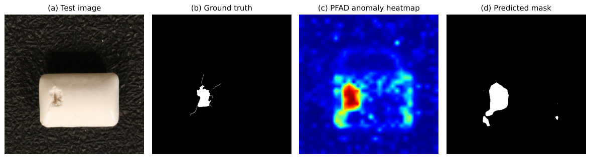
The performance pattern in Table 3 is consistent with a domain-gap analysis: under high domain gap (BTAD, only three categories with distinct visual statistics), the risk of channel activation collapse during transfer is greater, and Soft AFS provides calibrated per-channel weighting that mitigates this. Under moderate domain gap (MVTec AD ↔ VisA, both RGB texture datasets with 12–15 diverse categories), backbone features are already well aligned and the Soft AFS benefit is smaller. This pattern supports the design intent: Soft AFS is primarily a safeguard against domain-specific channel suppression rather than a general accuracy driver, and its value increases with the magnitude of the domain gap. Figure 2 shows representative qualitative segmentation results for the MVTec → VisA zero-shot setting.

4.3. Real Industrial Data

4.3.1. Semiconductor PCB Inspection (SemiCond)

PFAD generalizes effectively from public benchmarks to proprietary industrial data, achieving 0.945 image-level AUROC on semiconductor PCB inspection using only VisA as the training source (

Table 5. Cross-domain result: public benchmark → SemiCond semiconductor inspection (best configuration).

Source	Target	Img AUROC	Img AUPR	Pix AUROC	Pix AUPR
VisA	SemiCond-RGB	0.945	0.980	0.944	0.463

).

The interaction between training configuration and domain gap is detailed in Section 4.4.3.

Direct cross-modal transfer within the SemiCond dataset achieves image-level AUROC above 0.92 in both directions (

Table 6. SemiCond cross-modality zero-shot transfer. Images are evaluated at $300\times 300$ px (native resolution; images are upscaled to $512\times 512$ as model input).

Source	Target	Img AUROC	Img AUPR	Pix AUROC	Pix AUPR
SemiCond-RGB	SemiCond-Mono	0.952	0.985	0.961	0.314
SemiCond-Mono	SemiCond-RGB	0.929	0.973	0.966	0.430

), demonstrating that a model calibrated on one sensor modality can be deployed on a complementary sensor without retraining.

4.3.2. Pharmaceutical Packaging Inspection (Pharma)

Pharma represents the largest domain gap relative to the public benchmarks (pharmaceutical blister packs vs. mechanical components). Pharma images are captured at a resolution of $1024\times 1024$, with defects occupying a small fraction of the image area. Full-image inference at $512\times 512$ causes severe defect miniaturization, rendering image-level classification unreliable (I-AUROC: 0.43–0.66, with the lowest value falling below random chance). We therefore adopt patch-level inference as the primary strategy: each image is divided into a $2\times 2$ grid at the original resolution, and position-specific memory banks capture spatially varying patterns.

Table 7. Pharma patch-level inference: zero-shot vs. one-shot (image-level metrics).

Source	Img AUROC		Img AUPR
	0-Shot	1-Shot	0-Shot	1-Shot
KolektorSDD	0.894	0.891	0.963	0.955
VisA	0.767	0.871	0.840	0.929
MVTec	0.782	0.839	0.861	0.913
BTAD	0.764	0.813	0.871	0.896

presents the primary Pharma results under patch-level inference.

For more distant sources (VisA, MVTec, BTAD), the one-shot extension closes the domain gap substantially in both metrics (largest Img AUROC gain: VisA $+10.4$ pp; largest Img AUPR gain: VisA $+8.9$ pp), indicating that the few-shot pathway is most effective when zero-shot transfer leaves substantial room for improvement. When the training source shares structural similarity with the target domain—as in the case of KolektorSDD, an industrial electrical-component inspection dataset—zero-shot performance is already near saturation (0.894 Img AUROC, 0.963 Img AUPR), and one-shot fusion provides negligible additional gain. Notably, KolektorSDD shows a marginal decline in both AUROC ($-0.003$ pp) and AUPR ($-0.008$ pp) with one-shot. KolektorSDD’s surface cracks share elongated structural morphology with the source domain’s knowledge base, explaining its high zero-shot baseline. Crucially, while MVTec and VisA feature structured, object-oriented scenes where a single normal template provides essential geometric anchors, KolektorSDD consists of continuous, stochastic surface textures. For such texture-matching scenarios, a single reference image captures only a specific instance of the normal pattern (e.g., particular grain lines or subtle illumination gradients), introducing unnecessary reference ambiguity against inherent stochastic texture variations and leading to a marginal precision loss at the operating threshold. This pattern parallels the asymmetric one-shot behavior observed on SemiCond (Section 4.5.1); both cases are discussed jointly in Section 5.

Full-image inference at $512\times 512$ yields unreliable image-level results (I-AUROC: 0.43–0.66) due to severe defect miniaturization, further confirming that patch-level inference is the appropriate strategy for this domain.

4.4. Ablation Studies

4.4.1. Soft AFS vs. No AFS

Table 8. Effect of Soft AFS on cross-domain image-level performance (four representative pairs). Img AUROC: mean ± std over multiple independent seeds. Img AUPR: mean (std omitted; variance is negligible). Gap (Soft−No) is at most $0.11$ pp, within seed noise.

Source	Target	No AFS		Soft AFS (${\mathit{\tau }}_{\mathbf{afs}}$ = 0.1)
		Img AUROC	Img AUPR	Img AUROC	Img AUPR
VisA	BTAD	$0.9575\pm 0.0010$	0.990	$0.9576\pm 0.0010$	0.990
MVTec	VisA	$0.9169\pm 0.0021$	0.953	$0.9180\pm 0.0037$	0.955
VisA	MVTec	$0.9152\pm 0.0020$	0.936	$0.9153\pm 0.0019$	0.933
MVTec	BTAD	$0.9595\pm 0.0006$	0.986	$0.9596\pm 0.0006$	0.985
Mean		0.937	0.966	0.938	0.966

compares Soft AFS ($\tau =0.1$) against a No-AFS baseline (all channel weights fixed to one) across four representative cross-domain pairs.

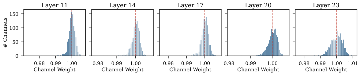
Soft AFS maintains comparable or superior performance on three of the four pairs (mean $+0.1$ pp in Img AUROC). The exception pair, VisA → MVTec (Img AUPR $-0.3$ pp; Img AUROC effectively unchanged at $+0.01$ pp), reflects the high intra-class diversity of VisA (12 categories spanning circuit boards to food products) as the source: calibration on such a broad feature space already approximates uniform channel weighting, leaving little room for Soft AFS to improve further. Multi-seed evaluation confirms that the gap is at most $0.11$ pp and falls within seed noise; No AFS and Soft AFS are statistically indistinguishable in both mean and variance (No AFS std $0.0020$ vs. Soft AFS std $0.0028$). Soft AFS is therefore retained not as an accuracy driver but as a zero-cost, stable component: calibrated, frozen weights add no inference overhead (feature dimension and head size unchanged; cf. Section 5) and are robust across ${\tau }_{\mathrm{afs}}$ and seeds (

Table 9. Ablation on AFS temperature ${\tau }_{\mathrm{afs}}$ (MVTec → VisA, CAA disabled, mean ± std over multiple independent seeds). AUROC is insensitive to $\tau$: the full sweep spans $0.18$ pp and the $\tau =0.01$ setting is statistically indistinguishable from $\tau =0.10$ ($\Delta =-0.16\pm 0.04$ pp). $\tau$ is folded into the frozen per-channel weights at calibration and acts as a robustness knob, not an accuracy lever. Note: The absolute AUROC reported here is lower than that in Table 10 (CAA enabled) because both $\tau$-sweep experiments were conducted under matched CAA conditions; the $\tau$-robustness conclusion holds under both settings.

${\mathit{\tau }}_{\mathbf{afs}}$	Img AUROC (Mean ± Std)
0.01	$0.9104\pm 0.0006$
0.05	$0.9090\pm 0.0005$
0.10	$0.9088\pm 0.0004$
0.50	$0.9086\pm 0.0004$
1.00	$0.9086\pm 0.0004$

). Figure 3 illustrates this mechanism: Soft AFS assigns each of the 1024 backbone channels a continuous weight proportional to its anomaly discriminability—channels whose activation patterns most closely track defect locations receive the highest weights. At $\tau =0.1$, learned weights occupy a narrow band (0.97–1.01 for large-scale sources), indicating that all channels contribute meaningfully while anomaly-relevant ones receive a calibrated boost. The BTAD source, with only three product categories, exhibits a slightly wider spread (0.90–1.03), consistent with more pronounced channel selection under limited source diversity.

4.4.2. AFS Temperature (${\tau }_{\mathrm{afs}}$)

Table 9 shows the effect of ${\tau }_{\mathrm{afs}}$ on cross-domain performance (MVTec → VisA, CAA disabled, mean ± std over multiple independent seeds).

Table 10. Sensitivity of Soft AFS to the temperature ${\tau }_{\mathrm{afs}}$ across four domain pairs, CAA enabled (Image AUROC, category-mean, mean ± std over multiple independent seeds). Sharpening from $\tau =0.10$ to $\tau =0.01$ changes AUROC by at most $0.10$ pp per pair (mean $\Delta =-0.01$ pp): Soft AFS is insensitive to $\tau$ regardless of whether CAA is used.

Pair	$\mathit{\tau }=0.10$	$\mathit{\tau }=0.01$	$\mathbf{\Delta }$ (pp)
MVTec → VisA	$0.9180\pm 0.0037$	$0.9171\pm 0.0013$	$+0.09$
MVTec → BTAD	$0.9596\pm 0.0008$	$0.9597\pm 0.0010$	$-0.01$
VisA → MVTec	$0.9153\pm 0.0019$	$0.9164\pm 0.0023$	$-0.10$
VisA → BTAD	$0.9576\pm 0.0013$	$0.9576\pm 0.0013$	$+0.00$
mean			$-\mathbf{0}.\mathbf{01}$

extends this analysis across four domain pairs with CAA enabled, confirming the $\tau$-robustness finding holds broadly.

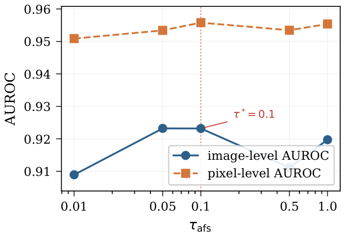
The ${\tau }_{\mathrm{afs}}$ sweep spans only $0.18$ pp (from $\tau =0.01$ to $\tau =1.00$), confirming that AUROC is insensitive to the temperature parameter. This robustness arises because $\tau$ is folded into the frozen per-channel weights at calibration time: the direction vectors learn to compensate for the channel weighting regardless of sharpness, so moderate sharpening neither helps nor hurts. We select ${\tau }_{\mathrm{afs}}=0.1$ as the default, which provides a non-trivial but non-degenerate calibration signal while remaining robust to perturbations. Figure 4 visualizes the flat response across $\tau$.

4.4.3. Effect of Class-Aware Augmentation (CAA)

On public benchmarks, CAA ON yields modest improvements (

Table 11. Effect of CAA on public benchmark cross-evaluation (mean of 6 pairs).

Setting	Img AUROC	Img AUPR	Pix AUROC	Pix AUPR
CAA ON	0.924	0.952	0.938	0.418
CAA OFF	0.911	0.942	0.935	0.389

). However, on real industrial data (SemiCond), CAA OFF consistently achieves higher pixel-level AUROC. We attribute this to AFS calibration contamination: when CAA is enabled, augmented images alter the normal feature statistics (${\mu }_{\mathrm{normal}}$) and channel MSE scores, causing AFS to prioritize channels responsive to augmentation artifacts rather than real defects. This effect is amplified under large domain gaps.

To determine whether the entanglement is structurally harmful, we implemented and evaluated a decoupled pipeline: Phase A calibrates Soft AFS on an unaugmented loader (CAA disabled) and freezes the weights $w^l$; Phase B then trains $W_{\mathrm{cls}}$ and $W_{\mathrm{seg}}$ on the standard CAA-augmented loader with identical hyperparameters.

Table 12. Decoupled CAA ablation: Image AUROC (category-mean, a single representative seed). Paired t-test across categories (entangled vs. decoupled): $p>0.05$ on all pairs, indicating the entanglement is harmless in practice.

Configuration	MVTec → VisA	VisA → MVTec	MVTec → BTAD	VisA → BTAD
No AFS/No CAA	0.9050	0.9137	0.9627	0.9550
Soft AFS/No CAA	0.8961	0.9166	0.9642	0.9529
Soft AFS/CAA (entangled)	0.9219	0.9174	0.9604	0.9570
Soft AFS/Decoupled CAA	0.9185	0.9174	0.9603	0.9572
Paired t-test (entangled vs. decoupled, across categories): $p=0.320$    $p=0.390$    $p=0.423$    $p=0.303$

reports the four-configuration ablation.

The paired t-tests yield $p>0.05$ on all four pairs, confirming that decoupling AFS calibration from CAA does not materially change results. We do not claim a performance improvement from decoupling; the contribution of this experiment is to demonstrate that the CAA–AFS entanglement is harmless in practice.

4.5. Few-Shot Extension Results

4.5.1. SemiCond Cross-Modality Paired 1-Shot

When a spatially aligned normal reference image is available from the target sensor, the few-shot extension yields asymmetric cross-modality results on the SemiCond dataset (

Table 13. SemiCond cross-modality one-shot paired results.

Source	Target	Img AUROC	Img AUPR	Pix AUROC	Pix AUPR
SemiCond-RGB	SemiCond-Mono	0.890	0.903	0.960	0.337
SemiCond-Mono	SemiCond-RGB	0.977	0.990	0.977	0.471

), improving Mono → RGB transfer while degrading RGB → Mono transfer.

With a single paired reference image, the Mono → RGB direction reaches image-level AUROC of 0.977 ($+4.8$ pp over the zero-shot baseline of 0.929 in Table 6), indicating that even a single spatially aligned reference image provides sufficient information to bridge the sensor modality gap. The benefit is asymmetric across directions: the RGB → Mono direction declines from 0.952 (zero-shot) to 0.890 under one-shot fusion, suggesting that when the zero-shot baseline is already high, a single reference image can introduce modality-specific over-anchoring rather than further improvement. This asymmetry indicates that the one-shot pathway is most beneficial when the zero-shot performance leaves meaningful room for improvement.

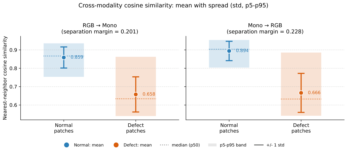
To investigate the mechanistic basis of this asymmetry, we conducted two diagnostic experiments on the SemiCond cross-modality dataset. First, photometric normalization of the reference image (Z-score, CLAHE, and histogram matching) did not improve Color → Mono performance, confirming that brightness or contrast differences between sensor modalities are not the underlying cause. Second, patch-level cosine similarity analysis revealed a structural feature-space asymmetry: normal patches in the Color → Mono direction achieve a mean nearest-neighbor cosine similarity of 0.859 to the one-shot memory bank, compared to 0.894 in the Mono → Color direction; defect patch similarities were comparable across both directions (0.658 vs. 0.666), indicating that defect discriminability was preserved, whereas normal-patch recall was impaired (Figure 5). This gap is consistent with a structural feature-space asymmetry induced by the RGB-pretrained backbone: DINOv3 likely exploits color-channel correlation information when processing RGB images, whereas monochromatic inputs (R = G = B) remove this cue, lowering patch-to-memory-bank similarity even for normal regions. As a result, 86.6% of normal SemiCond-Mono test images are misclassified as anomalous by the one-shot memory bank alone at the optimal image-level threshold, prior to zero-shot score fusion. Resolving this asymmetry would require feature-extractor-level cross-modal alignment, which is beyond the scope of the current retraining-free framework and is identified as a direction for future work.

4.5.2. Pharma Patch-Level 1-Shot

Patch-level inference and one-shot results for the Pharma dataset are reported in Section 4.3.2 (Table 7). For non-KolektorSDD sources, the one-shot extension improves image-level AUROC by up to 10.4 percentage points (largest: VisA $+10.4$ pp) and Img AUPR by up to 8.9 percentage points. KolektorSDD, as the domain-closest source, achieves the highest zero-shot performance (0.894 AUROC, 0.963 AUPR) with minimal one-shot benefit.

5. Discussion

Domain gap and transfer patterns. Cross-domain performance is positively associated with source dataset diversity. MVTec AD (15 categories) and VisA (12 categories) provide broader feature coverage than BTAD (three categories), resulting in more generalizable direction vectors. This finding suggests that curating diverse source datasets is a practical strategy for  deployment.

Segmentation robustness to domain gaps. Across all experiments, pixel-level AUROC degrades less than image-level AUROC under domain shift. In the extreme case of Pharma, pixel-level AUROC remains above 0.90 while image-level AUROC drops to 0.43–0.66. This finding suggests that local, patch-level anomaly patterns transfer more reliably than global, image-level representations, consistent with the observation that defects (scratches, stains, structural deviations) share low-level visual signatures across domains.

Soft AFS behavior. From a deployment perspective, the value of Soft AFS lies in its ability to provide calibrated channel importance without any inference overhead. Soft AFS provides a natural mechanism to absorb the uncertainty of domain transfer by retaining all channels with graded importance rather than discarding channels that may be critical in unseen target domains. The ${\tau }_{\mathrm{afs}}$ ablation (Table 9) shows that AUROC is insensitive to the temperature parameter: the entire sweep from $\tau =0.01$ to $\tau =1.00$ spans only $0.18$ pp under the current code (CAA disabled, multi-seed mean), with no significant penalty at any setting. This robustness arises because $\tau$ is folded into frozen per-channel weights at calibration time; the direction vectors compensate for any weighting sharpness. Direct comparison with a No-AFS baseline (Table 8) confirms statistical indistinguishability (mean gap $+0.1$ pp, within seed noise). The primary value of Soft AFS therefore lies in its zero-inference-cost, calibration-derived channel differentiation: it is never a liability and provides structural robustness to domain-specific channel shifts even when accuracy differences are not measurable on public benchmarks.

Few-shot as a practical bridge. The one-shot extension demonstrates that a single normal reference image can improve image-level classification when zero-shot performance has not yet reached saturation, but its benefit is domain-gap-dependent rather than universal. On Pharma, the largest domain gap scenario, one-shot inference improves image-level AUROC by up to 10 percentage points, with pixel-level performance remaining robust across all source configurations (consistent with the segmentation robustness patterns noted above). On SemiCond, paired one-shot cross-modality transfer can substantially improve one sensor direction (Mono → RGB reaches image-level AUROC of 0.977), but the effect is asymmetric and can become negative in the opposite direction when reference mismatch or modality-specific feature asymmetry is introduced. Two distinct mechanisms can cause one-shot fusion to underperform the zero-shot baseline: modality-specific over-anchoring, observed when the zero-shot baseline is already high (SemiCond RGB → Mono: 0.952 → 0.890, Table 13; see Section 4.5.1 for a mechanistic analysis); and reference ambiguity, observed when the source domain is already structurally close to the target (Pharma KolektorSDD: 0.894 → 0.891, Table 7). Both scenarios share a common operational implication: one-shot fusion should be applied selectively—it is most beneficial when zero-shot performance has meaningful headroom, not as a default addition to every deployment. Notably, this extension requires no additional training—only inference-time score fusion—making it a practical option when even minimal target-domain data is available. The results suggest a practical deployment rule: zero-shot transfer is appropriate when no target-side data are available; one-shot score fusion may provide additional benefit when a single normal reference image is available and zero-shot performance still has measurable headroom for improvement—when zero-shot is already near-saturated, the one-shot extension may offer little or no gain; and patch-level inference becomes necessary when defects occupy only a small fraction of high-resolution images.

Resource efficiency. PFAD trains only lightweight direction vectors on a frozen backbone, requiring no gradient computation through the backbone parameters. The entire training process is completed in approximately 18 min per source domain on a single NVIDIA RTX A6000 GPU. The measured inference efficiency (RTX A6000, batch 1, input $512\times 512$, 100 warm-up + 1000 timed iterations with torch.cuda.synchronize()): $61.44\pm 1.03$ ms/image, 16.28 FPS, peak VRAM 1.20 GB. For Pharma ($1024\times 1024$, $2\times 2$ patch split): 245.75 ms effective latency (4.07 FPS).

Table 14. Resource comparison. Energy estimated from GPU TDP × training time (not directly metered). UniADet latency (22.4 ms/image) is measured on an H20 GPU (their Table 4 [16]); direct speed comparison with our A6000 measurement is not valid due to hardware differences. Both operate in the sub-100 ms regime practical for end-of-line inspection.

Method	Train. Params	Train. Time	Latency (ms/img)	Peak VRAM
PatchCore [10]	0 (kNN) †	∼10 min	∼30 ms	∼3 GB
UniADet [16]	∼0.02 M	∼15 min	22.4 ms ‡	n/a
PFAD (ours)	0.02 M	∼18 min	$61.4\pm 1.0$ ms	1.20 GB

^† PatchCore stores patch features as a kNN coreset; training time = coreset build time (no gradient updates). Values are approximate benchmarks from [10] and community evaluations. ^‡ Measured on H20 GPU; not directly comparable to our A6000 measurement. Estimated energy: $\approx 0.09$ kWh/domain (300 W TDP × 18 min).

summarizes the resource profile.

Once trained, the model deploys to multiple unseen target domains without retraining, eliminating the repeated data collection and computation cycles that conventional per-domain models demand. AFS calibration leverages existing inspection records from the source domain rather than requiring new data campaigns. These properties collectively reduce the computational overhead and resource expenditure associated with deploying anomaly detection across diverse manufacturing lines. This is particularly relevant for factories operating large product portfolios, where repeated per-domain retraining amplifies GPU hours, engineering labor, and energy consumption over time. PFAD is parameter-efficient: only $\sim 0.02$ M direction vectors are trained on a frozen backbone, enabling domain adaptation without any retraining overhead; deployment on resource-constrained edge hardware would additionally require backbone quantization, which is left for future work.

Practical implications for industrial deployment. The experimental results directly support several concrete deployment benefits. Training on VisA alone yields an image-level AUROC of 0.945 on semiconductor PCB inspection without any target-domain data, demonstrating that an operator can deploy PFAD on a new inspection line immediately by selecting a suitable public source dataset—no proprietary data collection or retraining is required. When a representative normal reference image is available, the optional one-shot pathway can further reduce setup cost in favorable deployment settings, as illustrated by the Mono → RGB SemiCond result (image-level AUROC 0.977). However, as shown in Section 4.5.1, this benefit is not symmetric across sensor directions and should therefore be treated as a conditional deployment aid rather than a mandatory step. On pharmaceutical packaging, zero-shot transfer from KolektorSDD achieves an image-level AUROC of 0.894, indicating that an industrially sourced training dataset suffices for a chemically distinct production domain. However, when the source dataset is structurally dissimilar to the target domain (e.g., VisA or BTAD sources yield 0.764–0.782 image-level AUROC on Pharma), operators should consider selecting a more compatible source or applying the optional one-shot pathway before deployment in safety-critical applications. The full training pipeline completes in approximately 18 min per source domain on a single NVIDIA RTX A6000 GPU, while only 0.02 million of the model’s 300 million parameters are trained, keeping the model footprint small and suitable for edge deployment. Source selection is therefore a key deployment decision: datasets sharing surface texture and defect morphology with the target domain (e.g., industrial component inspection datasets for semiconductor PCB or surface-crack inspection datasets for pharmaceutical packaging) tend to yield higher zero-shot transfer performance. From an operational perspective, PFAD follows a simple three-step deployment workflow:

• Select source: choose the public source dataset most structurally compatible with the target domain (surface texture and defect morphology are the key criteria).
• Train once: train on the source dataset ($\approx 18$ min on RTX A6000); the resulting model transfers to all target domains without further training.
• Optionally refine: if a single normal reference image from the target is available and zero-shot performance still has meaningful headroom, apply one-shot score fusion at inference time.

Across both semiconductor and pharmaceutical validation scenarios, the same PFAD architecture is transferred without target-domain retraining, demonstrating practical versatility across two structurally distinct industries.

Limitations and future work. (1) The CAA–AFS interaction, in which class-aware augmentation during training can contaminate the AFS calibration signal, is addressed in the current protocol by disabling CAA during cross-domain transfer to industrial target domains. The decoupled-pipeline experiment (Table 12) shows no statistically significant difference between the entangled and decoupled pipelines ($p>0.05$ for all pairs when comparing entangled vs. decoupled pipelines). However, future architectural work could decouple these pipelines at the training level to recover the full benefit of CAA on source-domain benchmarks without adversely affecting cross-domain calibration. (2) The few-shot fusion weight ${\lambda }_f$ is currently fixed; adaptive fusion strategies conditioned on domain similarity could further improve performance. (3) Evaluation across a wider range of industrial domains and modalities would strengthen the evidence for generalizability. Additionally, an automated source-selection strategy that recommends the most transferable public source dataset for a given target production line would reduce the current reliance on operator knowledge.

6. Conclusions

This study demonstrates that target-domain retraining can be avoided when deploying anomaly detection on new industrial inspection lines: a benchmark-trained PFAD source model transfers directly to unseen production domains, and a single normal reference image further improves performance at inference time without any additional training. PFAD achieves this through Soft Anomaly-Aware Feature Selection applied to a frozen DINOv3 backbone. This mechanism preserves cross-domain transferability by retaining all feature channels with graded importance rather than applying hard channel selection. The absolute performance gain of Soft AFS over uniform channel weighting is modest (at most $+0.11$ pp image-level AUROC on public benchmark cross-domain pairs), with multi-seed evaluation indicating stable performance across random seeds. The benefit is most pronounced when the domain gap is large (e.g., BTAD: three industrial categories with distinct visual statistics). Validation on public benchmarks (mean image-level AUROC 0.924) and two real-world industrial datasets indicates the practical viability of the proposed framework. A single source model trained on a public dataset can be directly deployed for semiconductor PCB inspection without target-domain data collection, and the same framework transfers to pharmaceutical blister-pack inspection—a chemically and visually distinct production environment—without any per-domain retraining. When a single normal reference image is available and zero-shot performance has room for improvement, the optional one-shot extension can close domain gaps by up to 10 percentage points, enabling incremental adoption without retraining. By eliminating per-domain retraining, PFAD directly reduces the cumulative GPU computation, energy consumption, and engineering labor that conventional AD deployment demands at scale—costs that compound as facilities manage growing numbers of product lines or sensor configurations. These characteristics position PFAD as a practical contribution to sustainable manufacturing: a quality inspection capability that extends to new production environments without proportionally scaling its resource footprint, enabling broader adoption of AI-based inspection under real-world constraints on computational resources and personnel.

References

1. Shukla, V.; Shukla, A.; Prakash S. K., S.; Shukla, S. A Systematic Survey: Role of Deep Learning-Based Image Anomaly Detection in Industrial Inspection Contexts. Front. Robot. AI 2025, 12, 1554196. [Google Scholar] [CrossRef] [PubMed]
2. Ryalat, M.; Franco, E.; Elmoaqet, H.; Almtireen, N.; Al-Refai, G. The Integration of Advanced Mechatronic Systems into Industry 4.0 for Smart Manufacturing. Sustainability 2024, 16, 8504. [Google Scholar] [CrossRef]
3. Li, Z.; Yan, Y.; Wang, X.; Ge, Y.; Meng, L. A survey of deep learning for industrial visual anomaly detection. Artif. Intell. Rev. 2025, 58, 279. [Google Scholar] [CrossRef]
4. Bergmann, P.; Fauser, M.; Sattlegger, D.; Steger, C. MVTec AD—A Comprehensive Real-World Dataset for Unsupervised Anomaly Detection. In Proceedings of the 2019 IEEE/CVF Conference on Computer Vision and Pattern Recognition (CVPR), Long Beach, CA, USA, 15–20 June 2019; pp. 9592–9600. [Google Scholar]
5. Zou, Y.; Jeong, J.; Pemula, L.; Zhang, D.; Dabeer, O. SPot-the-Difference Self-Supervised Pre-Training for Anomaly Detection and Segmentation. In Proceedings of the European Conference on Computer Vision (ECCV), Tel Aviv, Israel, 23–27 October 2022; pp. 392–408. [Google Scholar]
6. Li, H.; Wang, X.; Liu, Y.; Liu, G.; Zhai, Z.; Yan, X.; Wang, H.; Zhang, Y. A Novel Robotic-Vision-Based Defect Inspection System for Bracket Weldments in a Cloud–Edge Coordination Environment. Sustainability 2023, 15, 10783. [Google Scholar] [CrossRef]
7. Chu, Y.; He, Y.; Xiong, X.; Lou, Y.; Yu, C. Augmented Hybrid Learning for Visual Defect Inspection in Real-World Hydrogen Storage Manufacturing Scenarios. IEEE Trans. Ind. Inform. 2024, 20, 8477–8487. [Google Scholar] [CrossRef]
8. Kandarkar, P.C.; Ravi, V.; Subramoniam, S.; Bijulal, D. Integrating Industry 4.0 and Sustainability Toward Attaining Smart Manufacturing Systems. Sustainability 2025, 17, 10674. [Google Scholar] [CrossRef]
9. Guo, L.; Lv, F. A Two-Stage Deep-Learning Framework for Industrial Anomaly Detection: Integrating Small-Sample Semantic Segmentation and Knowledge Distillation. Machines 2025, 13, 712. [Google Scholar] [CrossRef]
10. Roth, K.; Pemula, L.; Zepeda, J.; Schölkopf, B.; Brox, T.; Gehler, P. Towards Total Recall in Industrial Anomaly Detection. In Proceedings of the 2022 IEEE/CVF Conference on Computer Vision and Pattern Recognition (CVPR), New Orleans, LA, USA, 19–24 June 2022; pp. 14318–14328. [Google Scholar]
11. Guo, J.; Lu, S.; Zhang, W.; Chen, F.; Li, H.; Liao, H. Dinomaly: The Less Is More Philosophy in Multi-Class Unsupervised Anomaly Detection. In Proceedings of the 2025 IEEE/CVF Conference on Computer Vision and Pattern Recognition (CVPR), Nashville, TN, USA, 11–15 June 2025. [Google Scholar]
12. Jeong, J.; Zou, Y.; Kim, T.; Zhang, D.; Ravichandran, A.; Dabeer, O. WinCLIP: Zero-/Few-Shot Anomaly Classification and Segmentation. In Proceedings of the 2023 IEEE/CVF Conference on Computer Vision and Pattern Recognition (CVPR), Vancouver, BC, Canada, 17–24 June 2023; pp. 19606–19616. [Google Scholar]
13. Zhou, Q.; Pang, G.; Tian, Y.; He, S.; Chen, J. AnomalyCLIP: Object-Agnostic Prompt Learning for Zero-Shot Anomaly Detection. In Proceedings of the 2024 International Conference on Learning Representations (ICLR), Vienna, Austria, 7–11 May 2024. [Google Scholar]
14. Cao, Y.; Zhang, J.; Frittoli, L.; Cheng, Y.; Shen, W.; Boracchi, G. AdaCLIP: Adapting CLIP with Hybrid Learnable Prompts for Zero-Shot Anomaly Detection. In Proceedings of the 2024 European Conference on Computer Vision (ECCV), Milan, Italy, 29 September–4 October 2024. [Google Scholar]
15. Gao, B.; Zhou, Y.; Yan, J.; Cai, Y.; Zhang, W.; Wang, M.; Liu, J.; Liu, Y.; Wang, L.; Wang, C. AdaptCLIP: Adapting CLIP for Universal Visual Anomaly Detection. arXiv 2025, arXiv:2505.09926. [Google Scholar]
16. Gao, B.; Wang, C. One Language-Free Foundation Model Is Enough for Universal Vision Anomaly Detection. arXiv 2025, arXiv:2601.05552. [Google Scholar]
17. Oquab, M.; Darcet, T.; Moutakanni, T.; Vo, H.; Szafraniec, M.; Khalidov, V.; Fernandez, P.; Haziza, D.; Massa, F.; El-Nouby, A.; et al. DINOv2: Learning Robust Visual Features without Supervision. arXiv 2024, arXiv:2304.07193. [Google Scholar]
18. Simeoni, O.; Vo, H.; Seitzer, M.; Baldassarre, F.; Oquab, M.; Jose, C.; Khalidov, V.; Szafraniec, M.; Yi, S.; Ramamonjisoa, M.; et al. DINOv3. arXiv 2025, arXiv:2508.10104. [Google Scholar]
19. Zhang, X.; Xu, M.; Zhou, X. RealNet: A Feature Selection Network with Realistic Synthetic Anomaly for Anomaly Detection. In Proceedings of the 2024 IEEE/CVF Conference on Computer Vision and Pattern Recognition (CVPR), Seattle, WA, USA, 16–22 June 2024; pp. 16699–16708. [Google Scholar]
20. Jézéquel, L.; Beaudet, P.L.; Histace, A.; Vu, N.S. Unified Anomaly Detection via Multi-Scale Contrasted Memory. IEEE Trans. Image Process. 2026, 35, 2802–2815. [Google Scholar] [CrossRef] [PubMed]
21. Radford, A.; Kim, J.; Hallacy, C.; Ramesh, A.; Goh, G.; Agarwal, S.; Sastry, G.; Askell, A.; Mishkin, P.; Clark, J.; et al. Learning Transferable Visual Models From Natural Language Supervision. In Proceedings of the 2021 International Conference on Machine Learning (ICML), Virtual, 18–24 July 2021; pp. 8748–8763. [Google Scholar]
22. Liu, J.; Guo, M.; Cong, Y. Few-Shot Anomaly Detection via Personalization. In Proceedings of the 2024 Advances in Neural Information Processing Systems (NeurIPS), Vancouver, BC, Canada, 10–15 December 2024. [Google Scholar]
23. Zhu, J.; Pang, G. Toward Generalist Anomaly Detection via In-Context Residual Learning with Few-Shot Sample Prompts. In Proceedings of the 2024 IEEE/CVF Conference on Computer Vision and Pattern Recognition (CVPR), Seattle, WA, USA, 16–22 June 2024; pp. 17826–17836. [Google Scholar]
24. Liang, X.; Zhang, M.; Feng, G.; Wang, D.; Xu, Y.; Gu, F. Few-Shot Learning Approaches for Fault Diagnosis Using Vibration Data: A Comprehensive Review. Sustainability 2023, 15, 14975. [Google Scholar] [CrossRef]
25. Jiang, Y.; Cao, Y.; Shen, W. Prototypical Learning Guided Context-Aware Segmentation Network for Few-Shot Anomaly Detection. IEEE Trans. Neural Netw. Learn. Syst. 2025, 36, 12016–12026. [Google Scholar] [CrossRef] [PubMed]
26. Wang, S.; Han, Y.; Zheng, P.; Li, Y.; Wang, L. LOGIC-AD: Cross-domain zero-shot anomaly detection via logit-space consistency. Knowl.-Based Syst. 2026, 347, 116215. [Google Scholar] [CrossRef]
27. Lin, T.; Goyal, P.; Girshick, R.; He, K.; Dollár, P. Focal Loss for Dense Object Detection. In Proceedings of the 2017 IEEE International Conference on Computer Vision (ICCV), Venice, Italy, 22–29 October 2017; pp. 2980–2988. [Google Scholar]
28. Milletari, F.; Navab, N.; Ahmadi, S. V-Net: Fully Convolutional Neural Networks for Volumetric Medical Image Segmentation. In Proceedings of the 2016 Fourth International Conference on 3D Vision (3DV); IEEE: New York, NY, USA, 2016; pp. 565–571. [Google Scholar]
29. Mishra, P.; Verk, R.; Fornasier, D.; Piciarelli, C.; Foresti, G. VT-ADL: A Vision Transformer Network for Image Anomaly Detection and Localization. In Proceedings of the 2021 IEEE International Symposium on Industrial Electronics (ISIE), Kyoto, Japan, 20–23 June 2021; pp. 1–6. [Google Scholar]
30. Tabernik, D.; Šela, S.; Skočaj, J.; Skočaj, D. Segmentation-Based Deep-Learning Approach for Surface-Defect Detection. J. Intell. Manuf. 2020, 31, 759–776. [Google Scholar]
Figure 1. The PFAD framework: a representative MVTec → VisA zero-shot inference example. Solid arrows: zero-shot data flow (frozen DINOv3 backbone extracts multi-scale patch tokens; Soft AFS reweights channels; decoupled heads compute classification and segmentation scores; Score Fusion produces the final anomaly map). Dashed arrows: optional one-shot few-shot extension (Block E), in which a memory bank built from a single target-domain support image provides complementary anomaly scores fused at the score level. Purple dashed box: optional few-shot extension module (Block E). Blue borders: frozen modules; orange borders: trained modules.
Sustainability 18 06684 g001
Figure 2. Qualitative anomaly segmentation for MVTec → VisA zero-shot transfer (chewinggum category; category-mean pixel-AUROC = 0.996 , this representative image = 0.998 ). Panels: (a) test image, (b) ground-truth mask, (c) PFAD anomaly heatmap, (d) predicted binary mask (threshold = 0.5 of the min–max-normalized heatmap). Inter-method qualitative comparison is left for future work.
Sustainability 18 06684 g002
Figure 3. Soft AFS channel weight distribution across five backbone layers (source: VisA, τ = 0.1 ). Each channel i receives weight w i = softmax ( MSE i / τ afs ) × d , where MSE i scores how well channel i’s squared feature deviation aligns with ground-truth defect masks: channels with strong defect sensitivity (low MSE) are up-weighted above 1.0; less discriminative channels are mildly suppressed. For the large-scale VisA source, weights cluster in a narrow band (0.97–1.01), indicating near-identity calibration where all channels contribute. The BTAD source (three categories) exhibits a wider spread (0.90–1.03), reflecting more selective calibration under limited source diversity. The red dashed line at w = 1.0 marks the neutral weight threshold; # denotes number of channels.
Sustainability 18 06684 g003
Figure 4. Effect of AFS temperature τ afs on cross-domain performance (MVTec → VisA). The dashed line marks the optimal temperature τ * = 0.1 .
Sustainability 18 06684 g004
Figure 5. Patch-level nearest-neighbor cosine similarity distributions for the SemiCond cross-modality one-shot setting (updated to include distributional spread; shaded bands: mean ± std; whiskers: 5 th 95 th percentile). Normal patches: RGB → Mono (blue) shows mean 0.859 (std 0.057 , p 5 = 0.753 , p 95 = 0.936 ), shifted below Mono → RGB mean 0.894 (std 0.053 ), indicating structurally lower patch recall in the RGB → Mono direction; separation margin 0.201 . Defect patches: both directions show similar distributions (RGB → Mono mean 0.658 , Mono → RGB mean 0.666 ; separation margin 0.228 ), confirming defect discriminability is not impaired. The partial overlap of normal and anomaly p 5 p 95 bands in the normal-patch panel accounts for the elevated false-positive rate on normal images in RGB → Mono one-shot transfer (Section 5).
Sustainability 18 06684 g005