Article

Evidence-Based Land Degradation Assessment with Earth Observation Data Products

State Institution “Scientific Centre for Aerospace Research of the Earth of the Institute of Geological Sciences of the National Academy of Sciences of Ukraine”, Olesia Honchara Str., 55-B, 01054 Kyiv, Ukraine
*
Author to whom correspondence should be addressed.
Sustainability 2026, 18(13), 6681; https://doi.org/10.3390/su18136681
Submission received: 14 April 2026 / Revised: 17 June 2026 / Accepted: 22 June 2026 / Published: 1 July 2026
(This article belongs to the Section Sustainable Management)

Abstract

Land degradation (LD) is one of the most pressing environmental problems on a global scale, directly threatening ecosystem resilience, food security, and sustainable land use. Traditional methods used to assess land degradation are often limited by high labor intensity and insufficient integration of heterogeneous geospatial datasets. In this study, we propose an evidence-based approach to LD mapping that integrates multi-source Earth observation (EO) data products with the Dempster–Shafer theory of evidence. A geospatial data cube was constructed based on precipitation, soil moisture, terrain slope, land surface temperature, land cover transitions, vegetation productivity, and soil organic carbon indices. Our classification workflow combined expert knowledge with probabilistic evidence weighting to define LD classes at a regional scale, and our methodology was tested in the Kryvyi Rih Iron Ore Basin (Ukraine), a region under intense anthropogenic and natural pressure. Field-based validation demonstrated the high reliability of the proposed approach, achieving a Kendall rank correlation coefficient of 0.832, which outperforms alternative methods based on Support Vector Machines (SVMs) and Trends.Earth.

1. Introduction

Land degradation (LD) is recognized as one of the most pressing environmental and social problems on a global scale, directly threatening the sustainable development of society and ecological stability, with countless adverse effects on livelihoods and agricultural productivity [1,2]. A combination of natural factors, such as climate variability, drought, soil erosion, landslides, and wildfires, along with anthropogenic pressures like intensive land use, deforestation, increased pesticide and fertilizer use, water pollution, uncontrolled mining, and inadequate reclamation efforts, has led to the progression of this degradation. The consequences of land degradation cover both socio-economic and environmental spheres, going far beyond land systems. The loss of soil fertility, desertification, loss of biodiversity, decline in crop yields and food security, has increased losses in agribusiness, poverty and forced migration, and has reduced resilience to climate change all arise from land degradation [3]. All of these effects require timely, continuous spatial and comprehensive monitoring, as well as forecasting of land degradation trends, to reduce their associated risks. Traditional methods for assessing land degradation, including point datasets, visual assessments of soil condition, labor-intensive procedures, and laboratory methods, are limited in their assessment and consideration of integrative biophysical indicators. EO technologies are rapidly expanding, and the increase in available satellite data with various spectral and spatial capabilities has provided researchers with new opportunities for integrated environmental monitoring. All indicators that reflect environmental changes are being actively studied to better understand ecosystem dynamics, and their comprehensive assessment plays an important role in understanding these changes. However, there are still many methodological gaps in the development of a comprehensive approach that takes into account the heterogeneity of indicators, formalizes uncertainty, and presents this problem as a holistic, ordered, and categorical phenomenon. All existing land degradation modeling and assessment tools based on EO land degradation frameworks and SDG 15.3.1 operational tools consider degradation classes as nominal, and their impact weights are defined as fixed values for state indicators without a clear representation of uncertainty, and with conflicting information between EO indicators [4,5]. Solutions to the problem of obtaining comprehensive and transparent information to support decision-making remain limited, and the integration of heterogeneous datasets such as precipitation accumulation, soil moisture, land surface temperature, and gross dry matter productivity data into a spatially coherent and comprehensive framework remains largely unexplored.
Alternative methodological approaches, such as multi-criteria decision analysis (MCDA), machine learning methods, and time series trend analysis, partially solve the problem of data integration but have their limitations. MCDA approaches often rely on expert judgment but typically use static indicator weights and do not account for clearly contradictory or ambiguous information [6].
While support vector methods have demonstrated high predictive power in environmental impact-oriented land degradation mapping tasks [7], they typically treat degradation classes as nominal categories, do not account for their ordered nature, and provide limited transparency and interpretability for decision support. In addition, these approaches generally do not provide a unified mechanism for integrating heterogeneous environmental impact indicators, distributing uncertainty, and interpreting ordered degradation classes within a single operational methodological framework.
In this context, our proposed approach extends current practice in EO data cube analysis, which primarily focuses on statistical processing for feature detection. By integrating the Dempster–Shafer theory of evidence into the data cube analysis workflow, we improve the ability of this approach to model uncertainty and handle conflicting information when combining heterogeneous EO indicators.
Additionally, we formalize the inclusion of expert knowledge by describing interval classes and the reliability of indicators. Treating land degradation levels as an ordered set of classes and applying a rank-order accuracy assessment allows us to move from traditional pixel-based accuracy metrics to an assessment that is consistent with the ordinal semantics of degradation, thus fundamentally differentiating the proposed method from existing approaches focused on environmental impacts.
Early warning systems (EWSs) are increasingly recognized as key tools for managing degradation risks [8,9]. Although widely used in drought-prone countries, such systems are still underdeveloped in the European Union and neighboring regions. Existing EWSs mainly focus on generating risk maps or issuing warnings for specific threats such as agricultural decline [10], drought [11], soil erosion [12], or deforestation [13]. However, in order to be effective, EWSs related to LD must cover a full cycle, from monitoring to forecasting, warning, response, and knowledge dissemination [9].
In this study, we address this issue by introducing an evidence-based framework for LD assessment that applies the Dempster–Shafer theory of evidence to integrate heterogeneous EO indicators into a holistic classification model. This approach combines expert knowledge with probabilistic thinking, allowing for a more accurate and reliable identification of LD classes.
This research contributes to the EWALD Project, which explores the feasibility of observing and analyzing LD processes in the so-called “European Frontier”—regions near the EU where climate change and anthropogenic pressures are particularly acute. Ukraine, with its high industrial impact and diverse land use pressures, was chosen as one of the project’s test areas. The proposed workflow not only improves the reliability of LD detection but also supports the development of operational geospatial tools for monitoring Land Degradation Neutrality (LDN) in line with the 2030 Agenda for Sustainable Development [14].

2. Related Works

To enable the early detection of land degradation and ensure the effective monitoring of its progression, it is essential to identify its underlying predictors—commonly referred to as drivers. Based on an analytical review of the existing literature, a driver can be defined as a driving force of change, encompassing all factors that directly or indirectly contribute to alterations in natural systems [15,16,17,18,19,20,21,22].
A number of studies have aimed to define the most efficient LD indicators. Researchers [23] have investigated 70 LD indication candidates within nearly 1700 test sites. The Global Assessment of Land Degradation and Improvement (GLADA) technique involves using the annual NDVI-to-annual rainfall ratio, the net primary productivity (NPP) and accumulated temperature ratio, and NDVI-NPP correlation [24,25]. Since the dataset for this technique includes urban area masks, it does not consider anthropogenic pressure on landscapes and landscape changes. Some approaches [26] have included several land degradation assessment techniques (remote sensing-based methods, expert opinions, abandoned cropland methods, and land use/land cover (LULC) changes) and several indicators, including soil organic carbon (SOC), NPP, biodiversity, and fractional vegetation cover (FVC).
Such approaches are highly labor-intensive and challenging to implement, particularly under conditions of limited access to ground-truth validation sites. However, modern remote sensing technologies and the availability of extensive multi-year datasets have enabled the development of a detailed, multi-factor land degradation model.
To achieve this, it is essential to select the most representative degradation indicators from among the available geospatial products. These indicators can be classified into several groups:
  • Land use and land cover (LULC) data reflect the surface cover type and are related to human activity and expanding anthropogenic pressure on ecosystems and the regional thermal regime [27]. LULC data sources include CORINE Land Cover and Copernicus Dynamic World.
  • Climatic indicators are significant LD indicators that reflect general energy and water balance, which is crucial for identifying ecosystems’ vulnerability to degradation [28]. This type of data typically has a low spatial resolution (in the range of several kilometers) and includes key climatic variables of the study area, such as precipitation, near-surface air temperature, and soil moisture. Data sources include TerraClimate and ERA5.
  • Vegetation characteristics, which show the consequences of LD for ecosystems and land use, are represented by vegetation indices and bioproductivity metrics such as the MODIS Leaf Area Index, MODIS Vegetation Indices, MODIS Net Primary Production, Copernicus Vegetation Indices, and Copernicus Vegetation Primary Production [29].
  • Land surface temperature (LST) is related to energy balance, surface heat flux, vegetation cover density and evapotranspiration, water surface area, and anthropogenic pressure on ecosystems [30]. It is derived from thermal satellite imagery, e.g., Landsat LST, MODIS LST, and Copernicus LST.
  • Topographic characteristics represent surface relief and slopes, which are important for investigating soil erosion and water ecosystem shapes [31]. Surface topography data are based on digital elevation models, e.g., SRTM, ASTER GDEM, and ALOS World3D.
A typical methodology for LD assessment using EO involves investigating spatiotemporal cubes of analysis-ready low- and medium-resolution data [32]. Biogeophysical parameters of the land surface captured by EO systems are determined as LD indicators [33]. Primarily, LD indicators are related to soil and vegetation, although land cover, temperature, precipitation, and topographical features are also often considered [34].
Various methods of EO data cube analysis are used for land degradation assessment, including direct feature extraction from multispectral imagery and geospatial modeling [35], the examination of natural LD drivers with geographic information technologies [36], knowledge-based expertise [6], multi-source data fusion [37], deep learning data mining [38], long-term time series analysis [39], and the spatial integration of land degradation processes [40]. In Europe, the Trends.Earth unified technique is often applied for LD assessment [4] and considers three LD subindicators, established by the 2030 Agenda for Sustainable Development (SDG indicator 15.3.1): changes in land cover, land productivity, and soil carbon stock [14].

3. Materials and Methods

In this section, one of the possible implementations of EO data products for land degradation assessment is discussed. Compared to known methods, we (i) expand the set of LD indicators by using weather and climatic variables, including soil temperature and moisture, a more accurate indicator of vegetation productivity from Copernicus, and terrain slopes; (ii) modify the land cover type transition matrix to make it consistent; (iii) apply an advanced mathematical framework—the Dempster–Shafer theory of evidence—which more efficiently handles uncertain, incomplete, and contradictory data; and (iv) introduce an improved accuracy assessment metric—Kendall’s correlation coefficient—which takes into account the ordered nature of LD classes.

3.1. Study Area

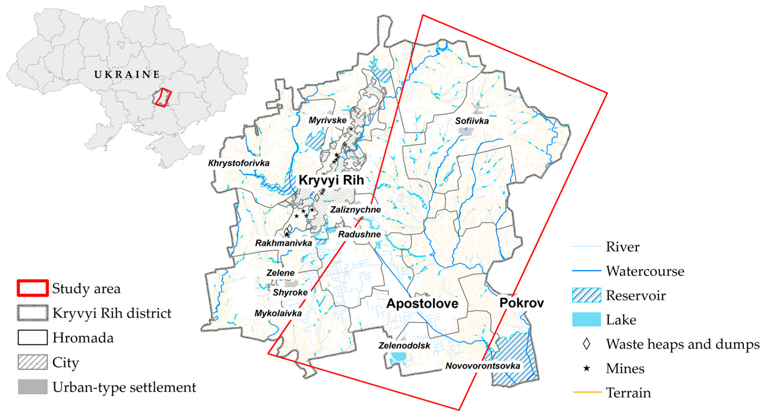
To study LD in an area of high industrial impact within the EWALD Project, a representative test region (TR) was selected in the center of the Kryvyi Rih Iron Ore Basin. The TR is delineated within the boundaries of the Kryvyi Rih district of Dnipropetrovsk Oblast in central Ukraine. Since the reform in July 2020, the district consists of 15 hromadas (municipalities), with an administrative center in the city of Kryvyi Rih. However, the focus of the present study was mostly on agricultural areas of the region, excluding ore mining and processing enterprises. The TR’s location and the overlapping area of interest are shown in Figure 1.
The study area is located in a temperate continental climate zone and belongs to the southern, arid, very warm agroclimatic region, with a fairly active atmospheric circulation, the predominant type of which is the westerly transport of air masses. In geomorphology, it is a steppe plain with a gentle slope to the south, a developed rafter–beam system, and clearly defined river valleys, which give the surface the character of a hilly steppe plain. The main physical–geographic processes that determine the natural relief formation are surface washing and, to a lesser extent, erosion.
Land degradation in the study area is caused by a range of natural and anthropogenic drivers that act either independently or in combination [41,42].

3.2. Assessment General Workflow

Designing a workflow for land degradation assessment and mapping is a non-trivial and challenging scientific problem. Due to the complexity, multifaceted nature, and ambiguity of land degradation processes, poorly structured and connotative scientific knowledge has become a primary and irreplaceable source for substantiating data analysis workflows [43]. The application of existing LD knowledge should be carried out in two main directions: a natural one—considering the causes, conditions, and drivers of LD—and an engineering one—enabling possibilities for the remote registration and evaluation of LD. By adopting this methodology, informal human expert involvement decreases, and it becomes possible to define an algorithmic workflow.
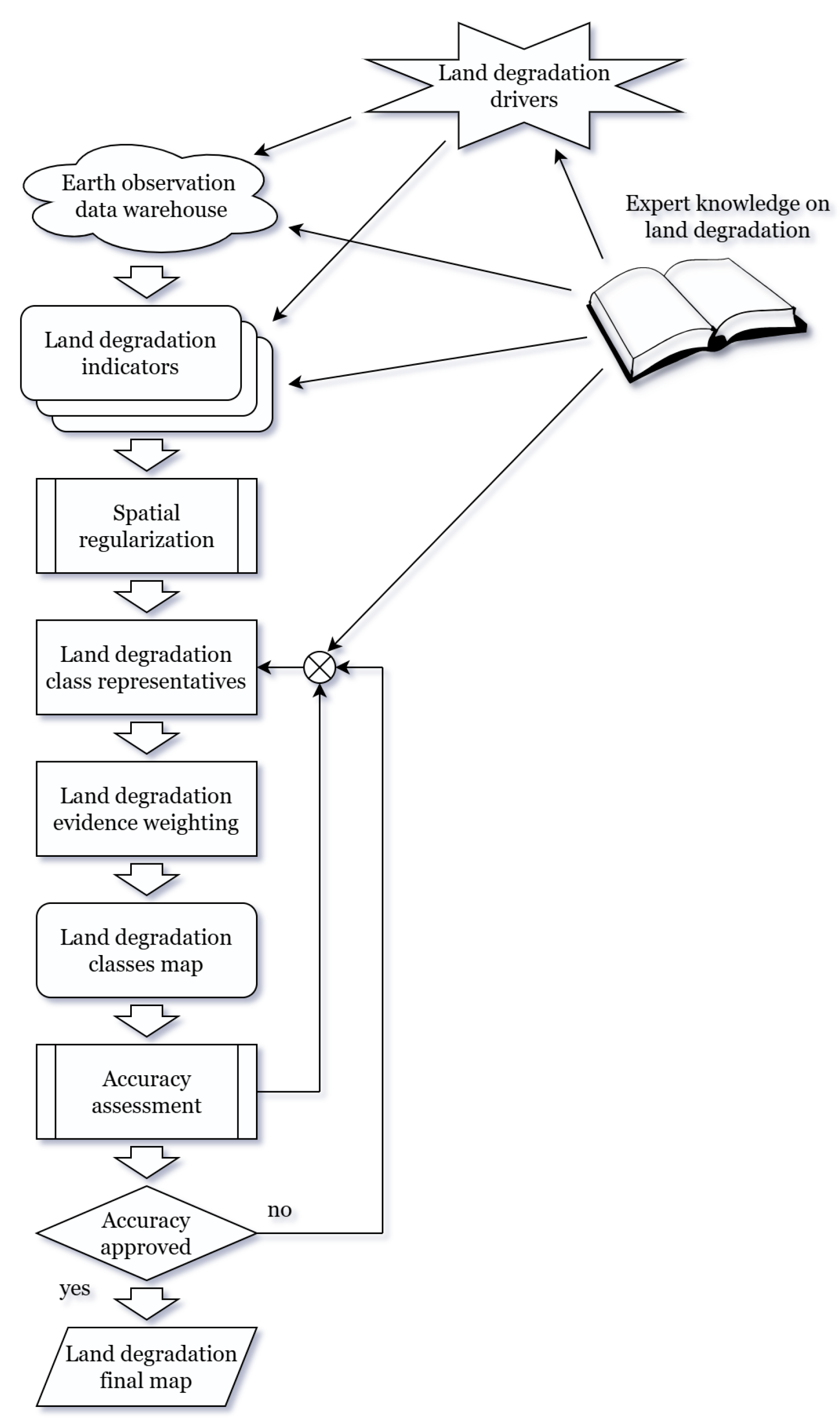
While many methods for LD mapping have been proposed, based on an equally vast variety of LD indicators [25], our approach is developed under the paradigm of supervised classification of the EO data cube [44]. The general flowchart of our technique for LD mapping is shown in Figure 2.
Natural knowledge of LD drivers and technical knowledge of available EO technologies jointly help to select a pool of LD indicators that (i) hold definitive significance and (ii) can be acquired remotely. As LD indicators, we do not consider direct remote sensing data, but rather consider analysis-ready geospatial data products that have undergone sophisticated task-oriented processing and modeling, usually higher than level 2 [45,46]. LD indicators should characterize biogeophysical parameters of the land surface, key landscape specifications, ecosystem conditions, long-term weather and climate impacts, and more. The creation of a processable data cube involves spatial regularization [47], specifically, equalizing the resolution of all data layers, aligning them to a common grid, filling in missing data, filtering/smoothing, applying masks, etc. This is followed by an inherent step in any controlled classification: expert-based specification of the LD class representatives for model training. Within the study area, experts select sites representing four land condition states: high degradation, moderate degradation, neutral condition, and remediation. The expression of these levels must be identified across all land cover types while accounting for study area heterogeneity. The experts responsible for selecting training and validation data must be qualified in land degradation assessment and satellite imagery interpretation and should have access to additional verification data for the study area.
In our study, a group of three experts performed the selection of robust intervals, taking into account the minimization of inter-expert variability.
A novel contribution of our workflow is LD evidence weighting, which accurately ensures the LD classification. The obtained LD class map usually requires refinement and adjustment for the specific study region. To achieve this, we employed two mechanisms: expert correction based on general knowledge and spatial correlation of the results with the training sample.

3.3. Land Degradation EO-Based Indicators

An important issue in evidence fusion is the potential mutual dependence of the indicators involved.
When forming the set of indicators, we aimed to select those that corresponded to LD drivers of varying physical natures, which were therefore essentially independent. Despite some outliers—e.g., a high correlation (0.77) between GDMP and SOC—the entire data cube remained weakly correlated, with an average correlation of −0.001. The correlation matrix for the entire data cube of LD indicators within the study area can be found in Appendix B.
Almost all of the LD indicators involved in the analysis reflected different primary LD drivers and, in our opinion, could be considered mutually independent. Additionally, the robust intrinsicality of the Dempster–Shafer combination led us to expect an acceptable result.
Since land degradation mapping requires several independent indicators, data cube generation involved the use of data from the following services: the Google Earth Engine (GEE) data catalog, the Copernicus Land Monitoring Service, and the Soils Grid service. Given that independence was a key criterion for indicator selection, other important comprehensive degradation indicators already included in the calculations of the above indicators were not considered—for example, the aridity index, which includes precipitation, or the erosion susceptibility indices, which include terrain slope data. Similarly, evapotranspiration-based indicators are also linked to precipitation and humidity and correlate with productivity, which are already accounted for by the above set of indicators.
The data cube contained seven data layers:
  • Precipitation accumulation data (mm) were derived from the TerraClimate geospatial product [48] and processed within the Google Earth Engine (GEE) environment using the “pr” band. The dataset was aggregated as the cumulative precipitation sum for the May–August period and had a spatial resolution of 4638.3 m.
  • Soil moisture data (mm), estimated through a one-dimensional soil water balance model and provided by the TerraClimate geospatial product [48], were processed in the GEE environment using the “soil” band. The variable was calculated as the mean soil moisture value for the May–August period at a spatial resolution of 4638.3 m.
  • Terrain slope data were generated from the 30 m spatial resolution Shuttle Radar Topography Mission (SRTM) digital elevation model dataset [49] within the GEE environment using the .slope() function, which converts elevation values into terrain slope angles.
  • Land surface temperature (LST) was estimated using long-wave infrared observations acquired by the United States Geological Survey Landsat 8/9 Level-2 Collection 2 geospatial product. LST was derived by converting the “ST_TRAD” radiance band into surface temperature using Planck’s law, while the standard emissivity band (“ST_EMIS”) was replaced with an NDVI-based emissivity estimation approach utilizing visible and near-infrared observations acquired by the same satellite platform [50]. The resulting LST dataset was calculated as the mean value for the May–August period at a spatial resolution of 30 m. The LST product used for land degradation (LD) mapping represented mean instantaneous Landsat-derived LST observations acquired at approximately 11:00 AM local time. Cloud and cloud-shadow masking was performed using the “QA_PIXEL” quality assessment layer.
  • Land cover transition data were derived from the Dynamic World V1 geospatial product available in the GEE data catalog. Dynamic World provides probabilistic land cover class predictions generated from Sentinel-2 Level-1C imagery with cloud cover ≤35% and a spatial resolution of 10 m [51]. Mean land cover class predictions for the May–August period were subsequently transformed into normalized land degradation impact scores using the analytic hierarchy process (AHP) technique [52].
  • Gross dry matter productivity (GDMP) data were derived from PROBA-V and Sentinel-3 OLCI observations [53]. The dataset, provided at a spatial resolution of 300 m with automatic exclusion of cloudy pixels, represents vegetation primary productivity in agro-statistical units of kg/ha/day. The final GDMP product was calculated as the mean productivity value for the May–August period.
  • Soil organic carbon (SOC) data, recognized as one of the principal land degradation indicators within the United Nations Sustainable Development Goal indicator framework SDG 15.3.1, were used to characterize long-term land degradation dynamics through an integrated assessment of land cover, land productivity, and SOC changes [5]. SOC data were obtained from the SoilGrids service at a spatial resolution of 250 m and expressed in t/ha across multiple soil depth intervals. For this study, SOC values calculated from the mean values of tree layers (0–5 cm, 5–15 cm, and 15–30 cm depth) were applied.
Some indicators were aggregated over the period corresponding to the peak vegetation activity, when productivity, as an LD indicator, is most sensitive to cumulative land conditions rather than short-term weather variability. For the study area, this covered the period from May to August.
Most of the data layers were obtained from analysis-ready data products, which already include standard preprocessing steps such as radiometric correction, cloud masking, gap filling, and temporal compositing, as provided by the original data producers. In some cases, scaling factors and offset values were applied to the datasets according to their official documentation. After selected data layers were downloaded and processed, they were co-registered and stacked into a data cube with a spatial resolution of 50 m. This resolution was selected as a compromise between the finest-resolution datasets (sourced from SRTM, Landsat, and Dynamic World) and coarser-resolution climatic products. Resampling was performed using bilinear interpolation, which is suitable for continuous environmental variables. Finally, the obtained data cube was spatially clipped to the study area and aligned to a common coordinate system for further analysis.

3.4. The Method for Evidence-Based Land Degradation Assessment

First, we will provide some notation and definitions. Let Ω be a set of objects described by a set of numerical features Π = π k k = 1 , K ¯ . The range of possible values of any of the k-th features is written as an interval-valued number π k = π _ k , π ¯ k , where π _ k and π ¯ k are the minimum and the maximum value of the k-th feature, respectively. Heterogeneous geospatial data are used as such features.
Our method is based on the principle of supervised classification, which assumes the presence of a training sample T = τ m m = 1 , M ¯ , where τ m is the training sample for class c m and M is the number of classes. Each object ω Ω belongs to one of the classes c m m = 1 , M ¯ .
Although the ultimate goal of this method is to determine the class of any object by its characteristics algorithmically, this goal is accomplished under the guidance of an expert. The expert’s functions include forming a training sample (dataset), selecting features, determining the relative importance of each, and post-classification refinement. The expert also determines the range of values for each selected feature based on the results of a statistical analysis of the characteristics of the objects of the training sample.
The task is to determine the class of any object ω Ω by its characteristics algorithmically.
Let us proceed to a description of the proposed method. The task of classifying objects based on heterogeneous geospatial data is solved by sequentially performing the following steps:
Step 1. Formation of the training sample: Representative objects are selected from the set Ω, that is, objects whose class membership is known a priori or can be established in some way at this step. From these objects, a training sample T = τ 1 τ m τ M is formed, where τ m is a subset of representative objects of the n-th class.
When forming the set S, attention is drawn to the fulfillment of the following requirements [54]:
  • In terms of the number of elements, the training sample T must have a volume that ensures the correctness of statistical estimates of classification accuracy.
  • For all classes, the subsets of representatives must have a power close in magnitude. When forming the set S, attention is drawn to the fulfillment of the following requirements, i.e., τ 1 τ m τ M .
Based on the analysis of the characteristics of the objects included in the training sample T, a dataset is constructed.
Step 2. Dataset construction: In our case, the dataset is a distribution of feature values inherent in each class. Based on our analysis of the properties of the objects of the training sample, the boundaries of the full range of its features’ π k k = 1 , K ¯ possible values are set on a scale from minimum π k min = min π k , 1 ¯ , , π k , m ¯ , , π k , M ¯ to maximum π k max = max π k , 1 ¯ , , π k , m ¯ , , π k , M ¯ .
Within the range Δ π k = π k max π k min for each feature π k k = 1 , K ¯ , based on additional information, the zone of values Δ π k , m = π k , m max π k , m min inherent in the corresponding class m = 1 , M ¯ is determined.
Thus, a dataset is constructed where the zones of possible values for each of the K features inherent in objects of different classes from c 1 to c m are recorded by the corresponding interval-valued numbers:
D a t a s e t = π k , m = π k , m ¯ , π k , m ¯ k = 1 , K ¯ ; m = 1 , M ¯ ,
Step 3. Intervalization of feature scales: While each zone within the full range of values of any feature is generated by a specific class and reflects it, it is necessary to take into account that zones generated by different classes can intersect with each other. Such intersections form additional interval zones on the numerical scale of the feature. Each additional interval zone is associated with the classes that formed it. If there are M defining zones (by the number of classes) on the feature scale, up to 2 M 1 various combinations of interval zones can be formed as a result of intersections. Each interval zone is recorded with the corresponding interval-valued number. That is, as a result of intervalization of the feature scale, its description can consist of 2 M 1 interval-valued numbers. This statement is valid for all K features.
Step 4. Normalization: The range of possible values of each feature is reduced to the interval [0, 1] by the equation
Δ π k   n o r m = π k π k min π k max π k min ,
where k = 1 , K ¯ .
Step 5. Formation of the basic probability assignment (BPA): Let the result of the measurement of the kth feature of the classification object be the value ξ k . In interval form, this number can be written as ξ k = ξ k , ξ k .
Then, the formation of the BPA for the kth feature is carried out in the following order:
1. Using the similarity equation, pairwise similarities between the result of the measurement of the kth feature, i.e., the interval-valued number ξ k , and the interval-valued numbers π k q are calculated. However, if we are dealing with an interval-valued number and a crisp number, then standard distance or similarity formulas for two interval-valued numbers may not be sufficient. Thus, before measuring the similarity between any crisp number and interval-valued number, we need to identify the key points we want to achieve.
Let a = a 1 , a 2 and b = b 1 , b 2 be two interval-valued numbers. If a is a crisp number, then the midpoint (center of the interval) m a = a 1 and its width w a = 0 . The only thing that we can operate now is the interval-valued numbers themselves, which hold only the start and end points of the intervals. In a classification process, we will be given a single pixel value, and the task will be to assign a confidence value to each classification class, which will enable us to answer the question “To which class does the pixel belong?”. This process will be repeated for each given layer of the source data (e.g., temperature, soil moisture, biomass). While there are many ways to provide such a value by comparing two intervals [55], none of them are suitable when we are dealing with a crisp and an interval-valued number comparison. Thus, we propose another approach to measure the similarity between a crisp number and an interval-valued number, which is based on the following key ideas: the similarity measurement should operate only with available data—that is, the start and end points of the interval-valued number (for the crisp number, the start and end points are the same value) and their derivatives:
  • The similarity measurement value should be greater if the crisp number is nested inside the comparing interval than the value if the crisp number value is outside the comparing interval.
  • The similarity measurement value should depend on the size of the interval. The broader the interval, the more uncertainty it contributes to the result.
  • Any crisp number can belong to the interval-valued number if it is outside of the interval-valued number. In this way, the source data intervals are not considered ideal.
For this task, we propose a specific similarity equation:
s a 1 , a 2 = 1 m a 1 , a 2 exp α m a 1 , a 2 w a 1 , a 2 2 / w a 1 , a 2 2 ,
where m a 1 , a 2 = m a 1 m a 2 is the distance between the centers of two interval-valued numbers, w a 1 , a 2 = w a 1 w a 2 is the difference between their length, and α is a variable parameter that controls the speed of the increment or decrement of function s (in this paper, α = 1.935). Thus, the justification of Equation (3) is now straightforward.
As one can see, we now have a function that rapidly increases if the crisp number is inside the interval and dramatically decreases if the crisp number is outside the interval boundaries with an exponential speed based on the interval size itself. Thus, a crisp number can belong to an interval even if it is outside of the interval boundaries. This value will be even greater if it is inside the interval and/or the interval-valued number length is small (for small intervals, there is less uncertainty, so the value will be bigger).
Physical interpretation (what is happening to the system)
  • Inside the interval, the system is stable or reinforced—the crisp number values are in the “allowed” region, so the function grows, reflecting that the system’s response is strong or amplified.
  • At the boundaries, the system experiences a sharp transition—crossing the boundary causes a sudden change in behavior.
  • Outside the interval, the system is suppressed or decays exponentially—the further the crisp number value moves away, the faster the system’s influence diminishes, meaning that the physical effect becomes negligible.
Thus, the following set is obtained:
s ξ k , π k 1 , , s ξ k , π k q , , s ξ k , π k 2 M 1 ,
2. The BPA distribution for the scale of the kth feature is formed as a set of basic masses:
B P A k = m k , 1 ,   ? . . , m k , q , m k , 2 M 1 ,
where m k , q = s ξ k , π k q / q = 1 2 M 1 s ξ k , π k q .
Similarly, BPAs are formed for all other features.
Step 6. Discounting the BPA: The purpose of BPA discounting is to prioritize their influence on the combination result. This influence is followed by the indicator significance index.
According to the postulate of pattern recognition theory, less class overlap inside the feature space provides a higher classification accuracy [56]. This postulate is a reason to assign higher significance to features with low inter-class interval overlap.
Considering indicator significance ensures the stability of the combination process, including in conflicting data cases [57].
First, a table of all possible intersections between class intervals is constructed:
I n t e r s = Z o I i , j π k , i , π k , j k = 1 , K ¯ ; i , j = 1 , M ¯ ,
where
Z o I a 1 , a 2 = min a 1 ¯ , a 2 ¯ max a 1 ¯ , a 2 ¯ max a 1 ¯ , a 2 ¯ min a 1 ¯ , a 2 ¯ ,
is the zone of intersection (ZoI) of a 1 and a 2 .
The significance index a k of the kth feature is then calculated using the equation
α k = 1 1 M 1 i = 2 M j < i Z o I π k , i , π k , j ,
All significance indices a k , k = 1 , K ¯ are calculated using this method.
The significance index takes values in the interval from zero to one. The closer the value is to one, the greater the significance of this feature.
Given the significance of the features, discounting the BPA is carried out according to the discounting equation presented in Appendix A. Similarly, all K BPA distributions are discounted.
Step 7. Merging the BPA: By sequentially merging the BPA distributions according to the rule of Dempster (see Appendix A), a combined BPA is obtained. Calculations are performed, taking into account the mutual independence of the indicators.
Step 8. Decision-making: For each element of the combined BPA, the pignistic probability is calculated using the full integral level of the hypothesis support equation (see Appendix A), after which the pignistic probabilities are ordered by magnitude, and a classification decision is made in favor of the element of the combined BPA with the maximum pignistic probability.

3.5. Summary

Summing up, Section 3 presents an innovative approach to land degradation assessment using Earth observation data products, one that is thoroughly justified and elaborated upon in detail.
A comprehensive workflow is described, covering all stages of land degradation assessment, ranging from the formalization of expert knowledge to the acquisition of the final LD map. Significant attention has been paid to the selection of relevant land degradation indicators among the existing higher-level Earth observation data products, i.e., those that reflect specific geobiophysical parameters of the land surface. A total of seven EO land degradation indicators of various physical natures have been selected, which together provide a more or less complete overview of the geosystem’s condition. A robust evidence-based method adapted for land degradation assessment has been proposed and tailored into a concise algorithm.
Now, all the necessary knowledge and tools for the practical assessment of land degradation within a specific test region are available.

4. Results

A direct experimental application of the developed mathematical models was conducted to assess land degradation within the study area described in Section 3.1. These models were applied to the EO data cube generated for the Kryvyi Rih study region, using the algorithm described in Section 3.4, for seven selected heterogeneous indicators, including precipitation accumulation, soil moisture, terrain slope, land surface temperature, land cover transitions, gross dry matter productivity, and soil organic carbon. This is how the final land degradation classification map shown below was obtained.
In defining land condition classes, the authors relied on the study [23]. For each selected indicator, the range of possible values was grouped into four classes using existing classification systems—in particular, the European georeferenced soil database https://esdac.jrc.ec.europa.eu/resource-type/european-soil-database-soil-properties (accessed on 21 June 2026).
Assume that we have four intervals that represent four degradation classes: High, Moderate, Low, and None. In this case, the “High” degradation class corresponds to severe and often irreversible land degradation, characterized by strong declines in productivity and surface condition. Such lands, including arable lands, are primarily situated on steep ravine slopes or substantially sloping terrain. They are severely eroded by intensive runoff and are unable to sustain productive plant communities. This class also includes lands within open quarries. “Medium” degradation represents an intermediate stage of land deterioration. This class is generally characterized by decreased soil fertility, some loss of plant life, or lower crop production. Lands in this class are predominantly represented by arable lands on sloping terrains. “Low” degradation indicates minor declines in productivity or structural changes that are still potentially reversible. This class is primarily composed of arable lands situated on flat or gently sloping terrain. In the Land Degradation Neutrality framework, this class could be considered as a neutral condition, when land shows neither systematic degradation nor improvement. The “None” class represents areas with stable or improving ecosystem conditions, where vegetation productivity and surface characteristics remain within the range of natural variability. Such areas mainly include natural and semi-natural lands with dense vegetation cover, like forests, including riparian forests and shelter belts, floodplain meadows, and wetlands. In the Land Degradation Neutrality framework, this class could be considered as remediated, especially in the context of the respective land cover transition.
Interval data were derived from the training sample, which was constructed by an expert through the visual delineation of degradation areas for each class on satellite RGB imagery. Under the specified conditions of LD identification, the training sample assembled by experts comprised 6754 pixels. To reduce the influence of potential outliers, the data for each indicator were subsequently filtered by removing the lowest 5% and highest 5% of values independently. Thus, the resulting intervals represented the expected value ranges for each class and served as reference thresholds against which every pixel in the source data cube was evaluated. By comparing pixel values to their corresponding class ranges, the classification of land degradation was systematically achieved.
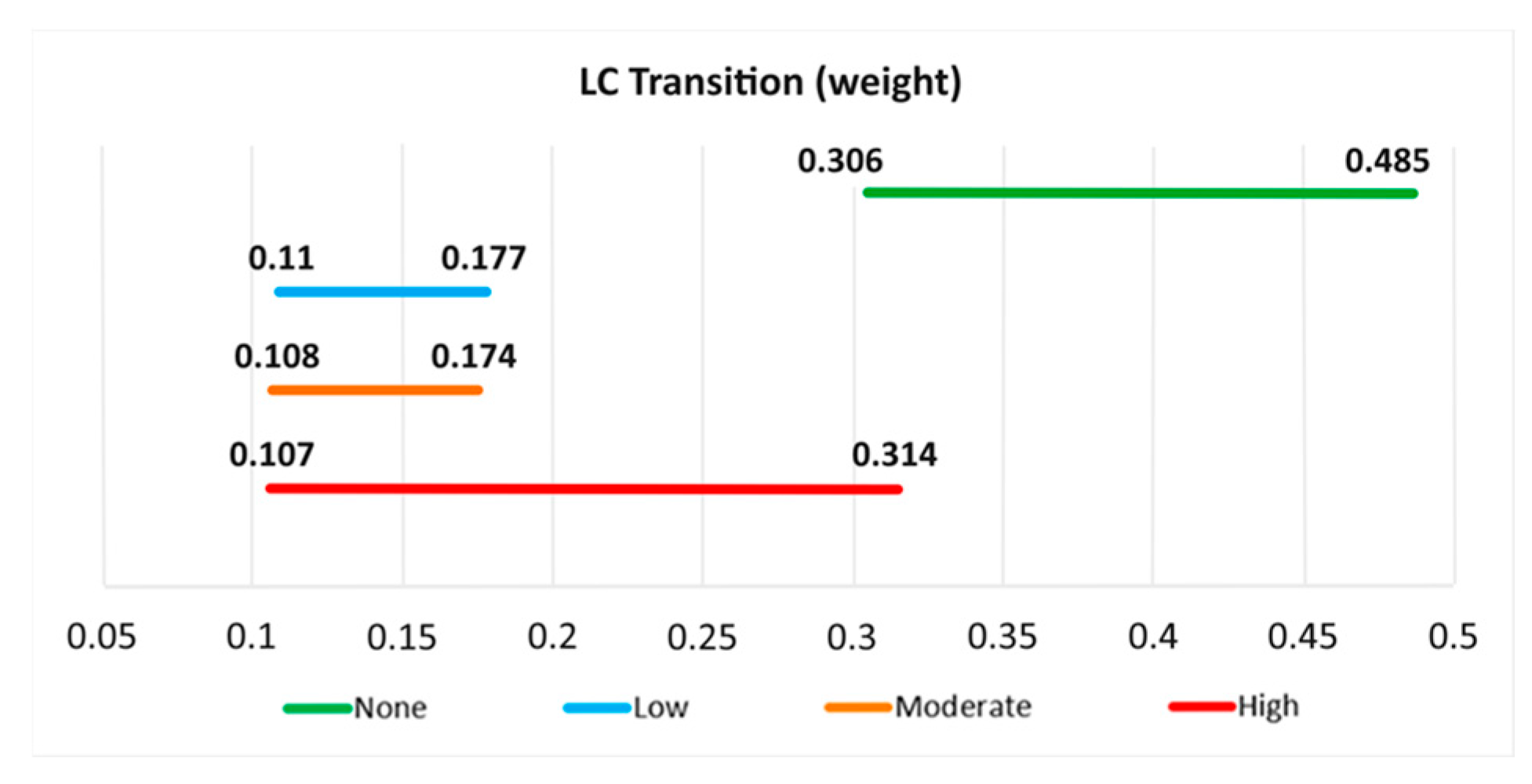
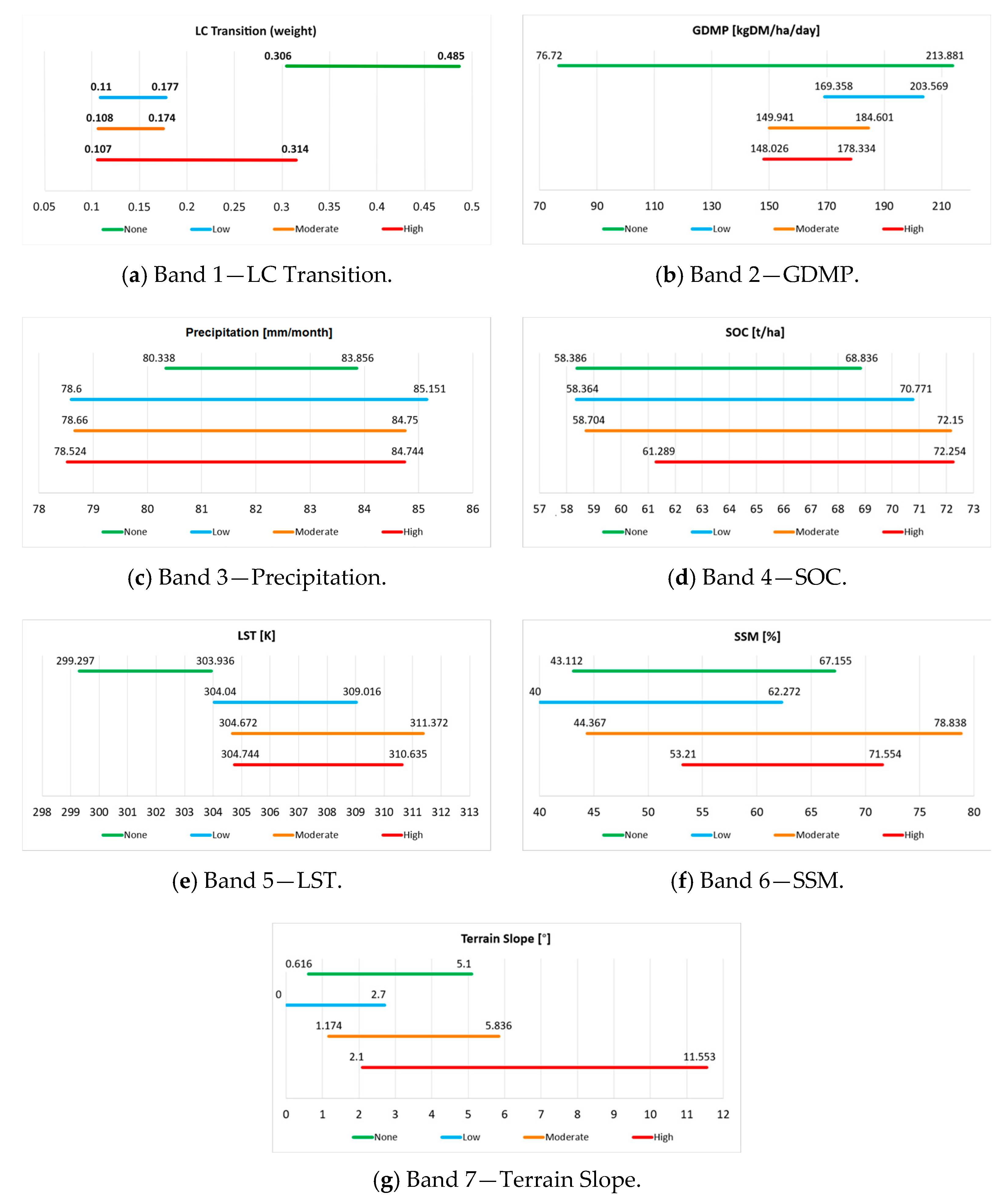
For demonstration purposes, the visual displacement of these interval-valued numbers, which are based on LC transition data, is shown in Figure 3.
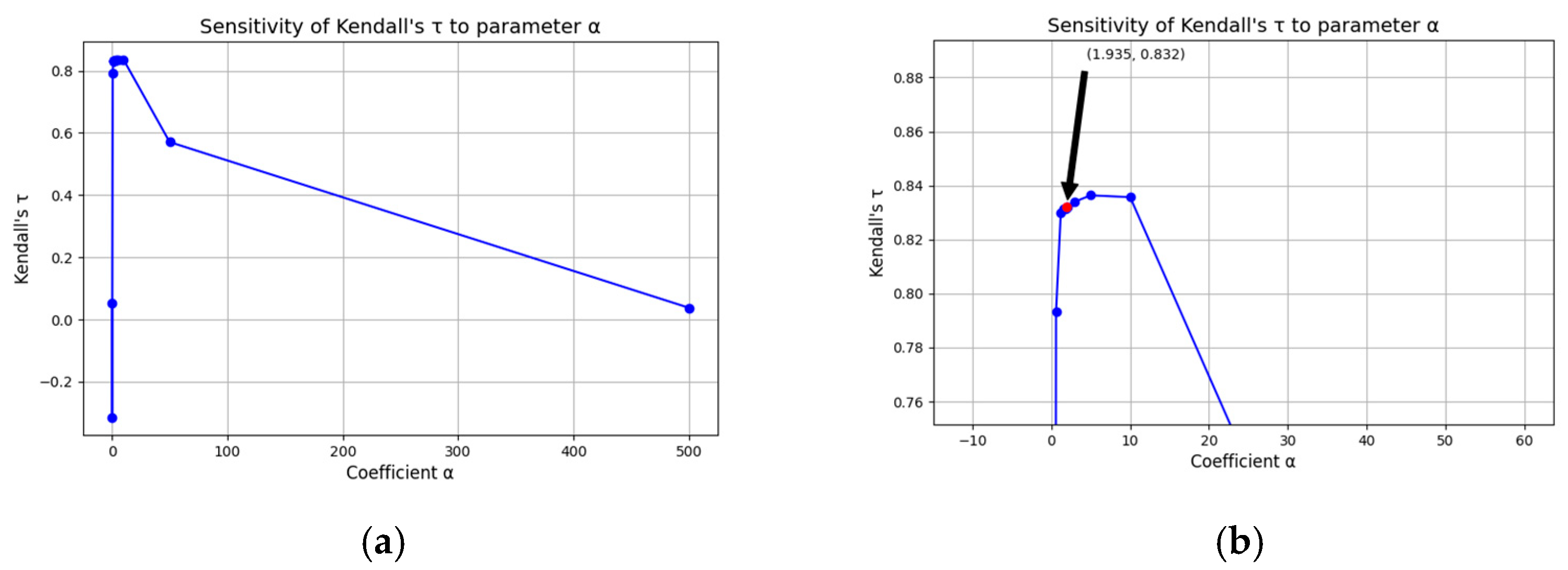
Our sensitivity analysis has shown that the optimal α value is in the range of 1–10. Considering the underlying rationale of Equation (3), this value should be rather low to make the decision less dependent on the difference between the mean interval value and the corresponding interval length. Thus, in our study, we used the value 1.935, whereas, in general, α = 2 is suggested. The sensitivity analysis is presented in Figure 4.
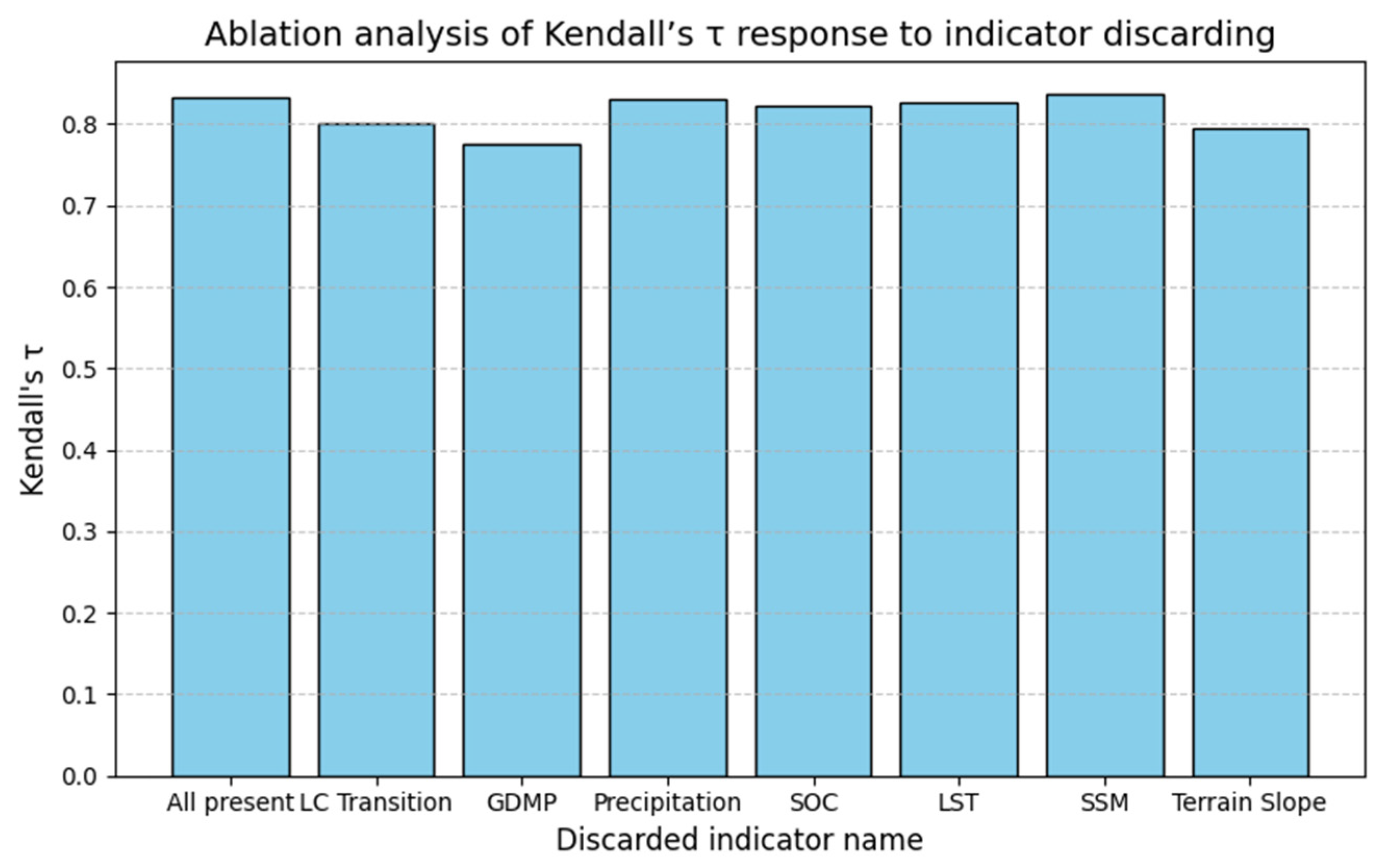
An ablation analysis was carried out by discarding indicators from processing one by one and comparing the Kendall’s τ coefficients. The discarding process was carried out by transforming the basic probability assignment of the respective indicator into a uniform distribution. The ablation analysis is presented in Figure 5.
As shown above, the discarding of surface soil moisture leads to a negligibly small increase in Kendall’s Tau. This could be due to low-quality SSM data, as these data have a low spatial resolution. Nevertheless, excluding this indicator may lead to a loss of completeness in hydrological indicators and in the representation of the associated processes.

Geoinformation Tool for Land Degradation Assessment

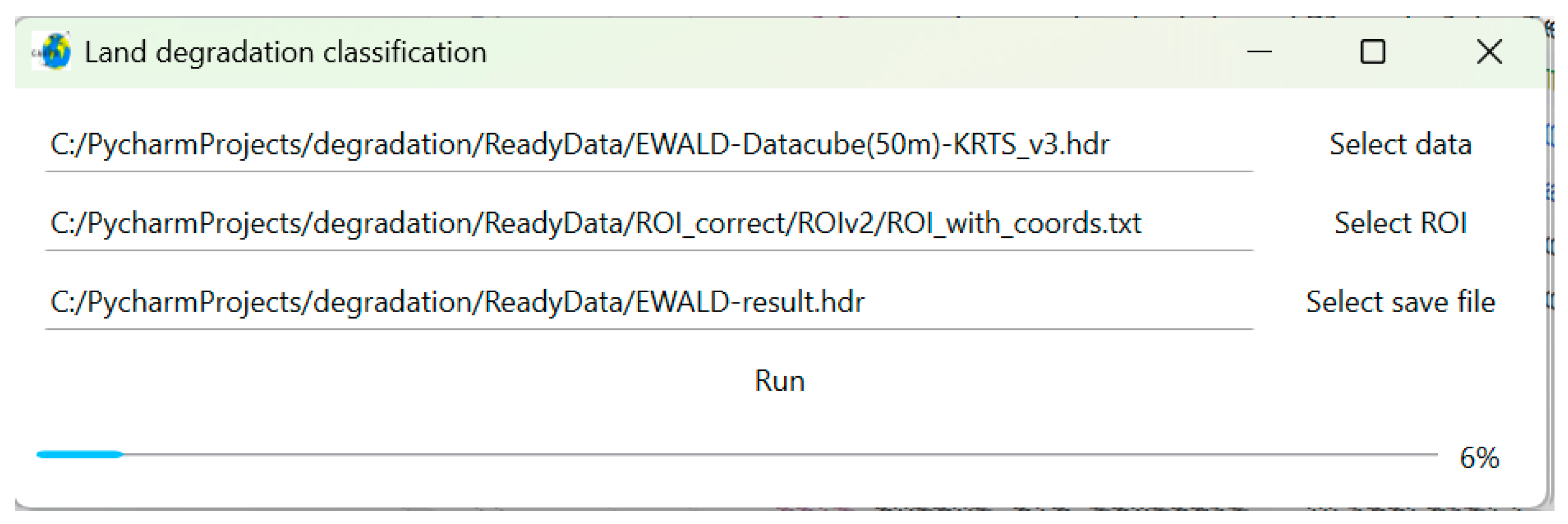
The classification approach described above was developed in the form of a special program using the Python (version 3) programming language and the free, open source libraries NumPy, SciPy, Matplotlib, and Spectral. The LD assessment processing workflow and an example of the developed graphical user interface (GUI) are given in Appendix C. The source code is available in the GitLab repository: https://gitlab.com/artur.r.lysenko/ldegradation (accessed on 21 June 2026).
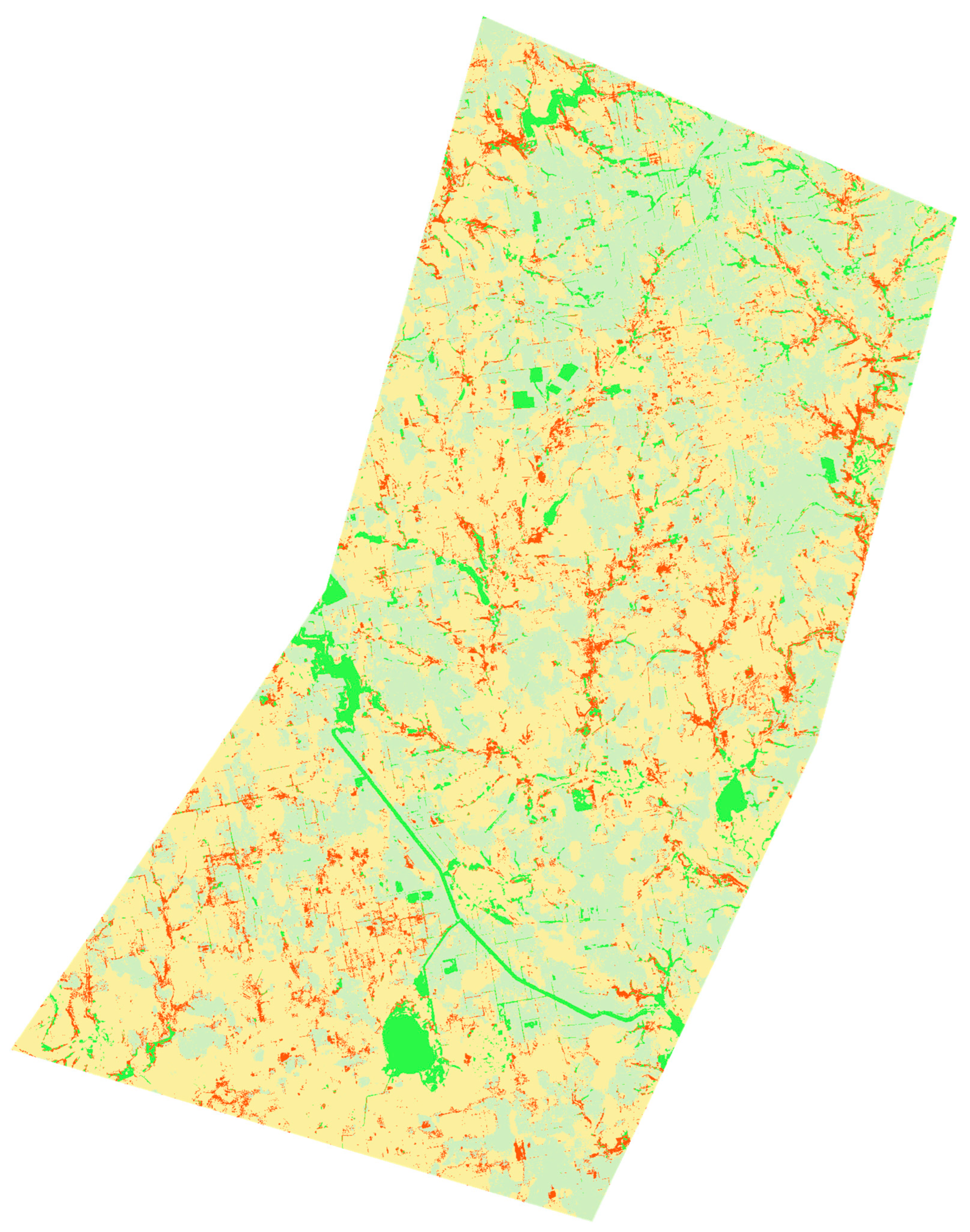
The program was tested on a computer workstation equipped with a 4.2 GHz 16-core CPU and 96 GB RAM. The processing time was ~13 min. Consequently, a land degradation classification map was generated, as illustrated in Figure 6.
LD classes were chosen based on the data discussed in Section 3.3, and the values of the visually identified and manually selected degradation class representatives were determined by an expert. Class intervals were built using training samples hand-picked directly from the data cube, as presented in Figure 7.
As shown above, this tool can be very convenient, considering that it requires only the value of the parameter α and the source data. However, the indicator generation process requires data from corresponding class representatives, which can be obtained from training samples based on real data.
The developed geoinformation tool will be valuable for local authorities, environmental agencies, and non-governmental organizations as an instrument for supporting management decisions in the fields of geoecology and land use, as well as for concerned citizens as a means of raising awareness about long-term geosystem trends.

5. LD Accuracy Estimation

A distinctive feature of the proposed approach for LD assessment and mapping is the categorical and ordered nature of the results, i.e., the LD classes. Traditional methods for classification accuracy assessment based on a confusion matrix [58] are not particularly suitable for LD maps. Rank-based assessment methods seem to be more relevant, as such methods are robust to errors, operable on small statistical samples, and adequately reflect the ordinal nature of the data [59].
In this study, we utilized Kendall’s rank correlation coefficient [60] as a metric for LD map accuracy estimation:
τ = 2 n ( n 1 ) i = 1 n 1 j = i + 1 n sign D i j ,
where D i j is the rank’s difference for elements i and j of the sample, positive or negative.
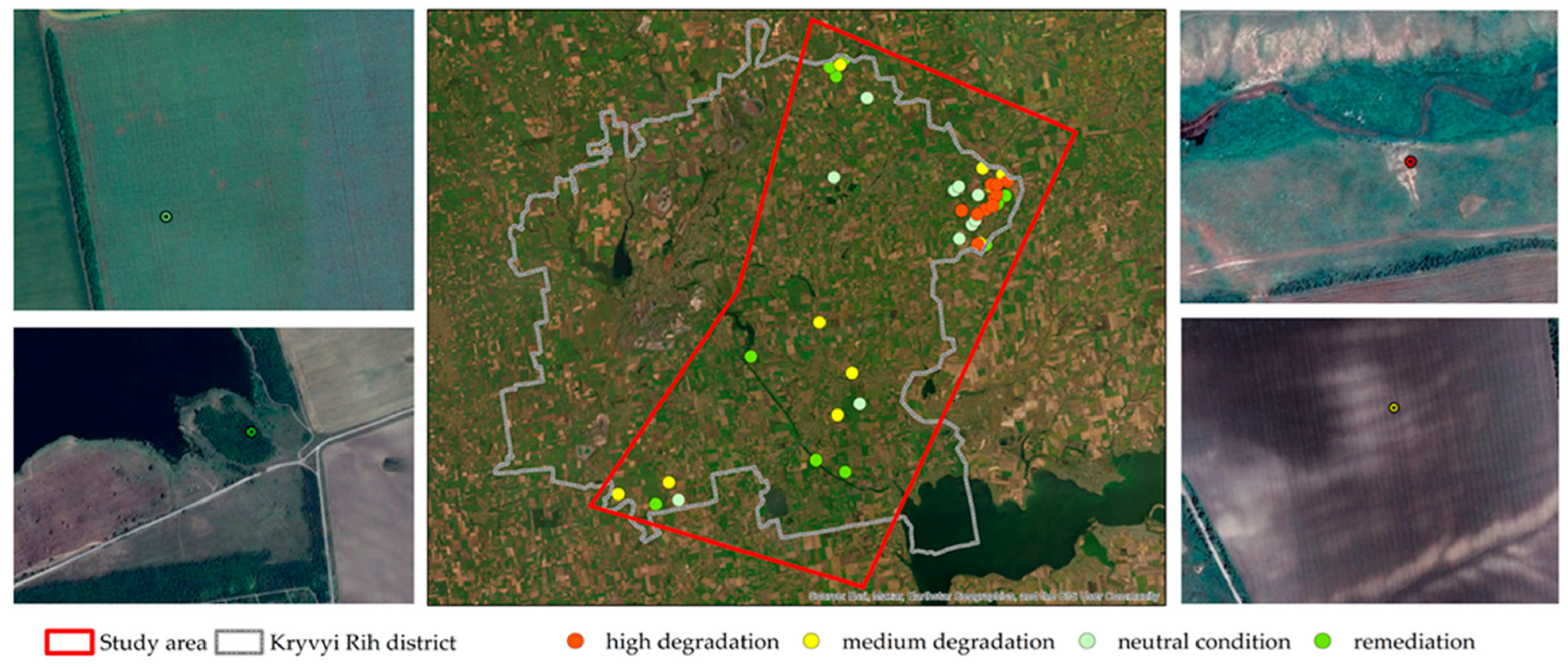
An approximately uniform sample of control points for all LD classes was obtained within the study area through direct observations by experts within interpretable sites, in parallel with the training data selection. In practice, the data selected by experts representing four predefined land condition classes were split into training and validation samples. Since the selected approach to LD is robust to small sample sizes and does not assume normality, the sample size was 40 control points (Figure 8). Nevertheless, this limited number of control points could restrict both the statistical power and spatial representativeness of the validation, and the results should be interpreted as indicative. However, with an increased amount of ground data, validation reliability may improve due to the better representation of land conditions in heterogeneous areas.
Thus, a stratified random sampling approach was applied to generate validation points and was performed with a disproportional distribution based on the regions of interest defined by an expert for each LD class.
Validation used ten points per class to ensure a reliable assessment of minority classes and a balanced evaluation of model performance across all degradation categories.
Using high-resolution GoogleEarth imagery, the generated validation points were visually interpreted to obtain the reference data for further accuracy assessment of the land degradation map. The control points were not included in the training samples.
The sample of control points was compared to the corresponding mapping results using Kendall’s correlation coefficient. For comparison, two competing techniques for LD mapping were assessed: SVM classification [7] of the same data cube and the Trends.Earth technique [61]. SVM classification was performed using a radial basis function (RBF) kernel. The gamma parameter was set to 1/7 (approximately 0.143), corresponding to the seven input layers used in the input geospatial data cube. Also, we used the same training sample that was used the proposed method. Since the SVM classifier was intended as a baseline comparative method, no exhaustive hyperparameter tuning or cross-validation was performed.
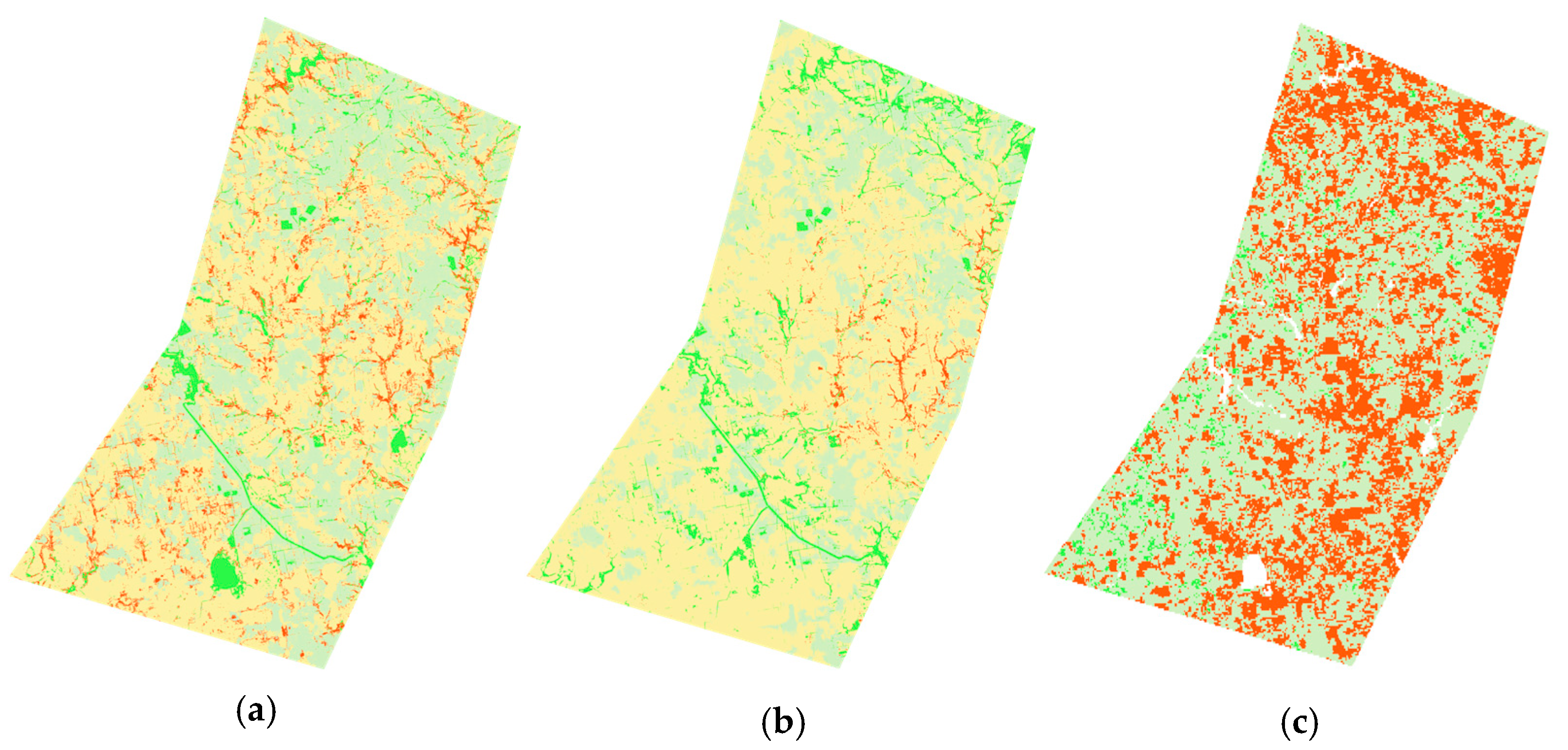
The assessment of SDG Indicator 15.3.1 was conducted using the Trends.Earth plugin within the QGIS environment using the UNCCD reporting preset. The selection of 2014–2017 as the baseline period and 2018–2022 as the reporting period is consistent with the Trends.Earth methodology. Both periods meet the minimum temporal requirements for SDG Indicator 15.3.1 estimation. The choice of 2022 as the end year is justified by data availability. For the overall baseline period, Trends.Earth estimates land productivity for SDG Indicator 15.3.1 by analyzing satellite-derived vegetation indices (NDVIs) to measure changes in biological productivity over time, incorporating data from MODIS and AVHRR. To calculate SOC changes, Trends.Earth uses SoilGrids 250m (top 30 cm) data and reclassified land cover maps, applying IPCC-recommended conversion coefficients based on land use transitions. A >10% reduction in SOC indicates degradation, while a >10% increase shows improvement. Land degradation status was determined through the integration of land productivity trends, LULC change, and SOC assumptions, following the “one-out, all-out” principle adopted for SDG Indicator 15.3.1. The rules governing transitions between LULC classes and their associated degradation or improvement outcomes are provided in Table 1. The mapping results are presented in Figure 9, while the values of Kendall’s correlation coefficient are provided in Table 2.
The confidence intervals for the obtained Kendall’s correlation coefficient values were also estimated. Since the sample size was n > 10, the confidence intervals were estimated using Fisher’s z-transformation [62]. The results are also included in Table 2. The IoU (intersection over union) metric between evidence-based and other competing techniques may indicate a meaningful superiority of the proposed technique over Trends.Earth and a non-significant one over SVM. In addition to the abovementioned accuracy metrics, we have also estimated the overall accuracy (OA) and the Kappa index. These values are presented for each of the three classifications in Table 2.
As indicated in Table 2, the evidence-based LD mapping technique slightly outperforms the alternative ones. A Kendall’s correlation coefficient value greater than 0.8 suggests a sufficiently close relationship between the obtained land degradation map and the actual land condition within the study area [63], at least over the limited sample.

6. Conclusions

A new evidence-based method for land degradation assessment has been proposed. Since land degradation is a complex and poorly formalizable phenomenon, it is assessed using a data cube with diverse biophysical parameters of the land surface, derived from satellite Earth observations, and the Dempster–Shafer theory of evidence, which more appropriately handles such data compared to traditional algorithms. In addition to the mathematical justification, a detailed algorithm and processing workflow for land degradation assessment have been developed.
While the algorithm and processing workflow were implemented using a conventional computation environment, further development of the proposed method, such as increasing the number of indicators involved or specifying a more detailed nomenclature of land degradation classes, will entail a high computational burden. Special algorithmic and software tools can be proposed for such cases, as in [64,65], for example.
The developed method was applied to assess land degradation within the test region defined by the EWALD international scientific project, namely, the Kryvyi Rih district of Dnipropetrovsk Oblast (Ukraine), situated in the center of the Kryvbas Iron Ore Basin. A Dempster–Shafer evidence-combining model was applied to integrate heterogeneous environmental state indicators, including precipitation, soil moisture, terrain slope, land surface temperature, vegetation productivity, land cover transitions, and soil organic carbon. Based on the proposed method, degradation hotspots in erosion-prone agricultural lands, disturbed industrial landscapes, and areas subject to long-term anthropogenic pressure were identified. A full-scale validation of the obtained land degradation map within the test region has been performed, and our statistical estimation results indicate the superiority of the proposed method over known equivalents, such as SVM classification and the Trends.Earth technique. The achieved Kendall correlation coefficient of 0.832 demonstrates that the mathematical model is not only theoretically sound but also operationally applicable in real environmental conditions.
The proposed methodology is not limited to the environmental conditions in Ukraine and can be adapted to a wide range of ecosystems and climatic zones. Since the approach is based on the flexible integration of EO-derived indicators derived from environmental impacts within the Dempster–Shafer evidence base, the set of indicators and threshold interval values can be calibrated to regionally specific degradation factors, ecosystem characteristics, and climatic conditions.
The proposed mathematical approach was experimentally implemented for the Zagora region in Morocco, another test region of interest within the EWALD Project [66], demonstrating the utility of the method for LD early warning in arid environments. In the Zagora region, desertification, which results from LD processes, is a problem where cultivated fertile irrigated lands can be transformed into waterless and lifeless deserts. The key outcomes of these LD processes are decreased soil fertility leading to vegetation and yield loss, resulting in further water scarcity, drought conditions, and aridization of soils; soil compaction; salinization due to high evaporation rates; and unstable water balance. The transferability of the methodology required adjustments, such as the calibration of EO indicators to local degradation drivers and the modification of temporal aggregation periods to match regional phenology. Therefore, such adaptations enabled the reliable assessment of LD across diverse environmental settings.
Further work should focus on improving the developed method, particularly on automatically adapting to the changed data cube and the objective weighing of the different indicators’ contributions to the aggregated assessment of land degradation. The method may also need to be updated when land degradation is assessed in other physiographic regions.

Author Contributions

Conceptualization, M.P.; methodology, M.P. and S.S.; software, A.A. and A.L.; validation, A.K. (Anna Kozlova) and A.A.; formal analysis, A.K. (Anna Khyzhniak); investigation, A.L. and M.L.; resources, A.A. and M.L.; data curation, M.L.; writing—original draft preparation, M.L.; writing—review and editing, M.P., S.S., and A.K. (Anna Khyzhniak); visualization, A.L.; supervision, M.P.; project administration, S.S.; funding acquisition, A.K. (Anna Khyzhniak). All authors have read and agreed to the published version of the manuscript.

Funding

This work was supported by the European Union under the Marie Skłodowska-Curie Actions (HORIZON-TMA-MSCA-SE—HORIZON TMA MSCA Staff Exchanges), part of the Horizon Europe programme, Grant agreement ID: 101086250.

Institutional Review Board Statement

Not applicable.

Informed Consent Statement

Not applicable.

Data Availability Statement

The data presented in this study are available from the corresponding author upon request.

Acknowledgments

The authors gratefully acknowledge the University of California, Merced, for providing the TerraClimate dataset. We also thank the United States Geological Survey (USGS) for access to Landsat data. We acknowledge the European Space Agency (ESA) and the Copernicus Programme for providing Sentinel-3 and PROBA-V satellite data. We further express our appreciation to the ISRIC—World Soil Information for making SoilGrids data on soil organic carbon (SOC) publicly available. The authors also acknowledge Google for providing the Google Earth Engine platform, which enabled efficient data access, processing, analysis, and exporting. This project has received funding from the European Union’s Horizon Europe research and innovation programme under the Marie Skłodowska-Curie Actions grant agreement No 101086250.

Conflicts of Interest

The authors declare no conflicts of interest.

Abbreviations

The following abbreviations are used in this manuscript:
EOEarth Observation
EWSEarly Warning Systems
FVCFractional Vegetation Cover
GDMPGross Dry Matter Productivity
GEEGoogle Earth Engine
GLADAGlobal Assessment of Land Degradation and Improvement
GUIGraphical User Interface
LCLand Cover
LDLand Degradation
LDNLand Degradation Neutrality
LSTLand Surface Temperature
LULCLand Use/Land Cover
MCDAMulti-Criteria Decision Analysis
NDVINormalized Difference Vegetation Index
NPPNet Primary Productivity
OAOverall Accuracy
SDGSustainable Goal Indicator
SOCSoil Organic Carbon
SSMSurface Soil Moisture
SVMSupport Vector Machine
TRTest Region
TSTerrain Slope
WPWater Precipitation

Appendix A. The Main Provisions of the Dempster–Shafer Theory of Evidence

In this appendix, we present the mathematical formulation employed in the study. Corresponding definitions are provided in Section 3.4. The core of the method for evidence-based land degradation assessment is founded on the following provisions of the Dempster–Shafer theory of evidence [67,68]:
  • The combination rule of Dempster is described by the following equation:
    m 1 m 2 A = B C = A m 1 B m 2 C 1 B C = m 1 B m 2 C ,
    where m 1 ( ) and m 2 ( ) are basic probability assignments m : 2 Θ 0 , 1 , and 2 Θ = , A , B , C , A B , A C , A B C , A B , Θ is a superset of hypotheses A, B, C, etc.
  • The discounting is carried out using the following equation:
    m α A = α m A | A ϵ 2 Θ , A Q 1 α | A = Q ,
    where α 0 , 1 and Q is the frame of discernment Θ = A , B , C , .
  • The full (integral) level of support for hypothesis A is calculated using the following equation:
    B e t P A = B A B 2 Θ A B B m B .

Appendix B. The Correlation Matrix of the LD Indicators’ Data Cube Within the Study Area

LCGDMPSOCWPSSMLSTTS
LC1.00.125−0.0210.0340.091−0.3450.197
GDMP0.1251.00.7710.411−0.6240.0270.039
SOC−0.0210.7711.00.556−0.6770.1570.031
WP0.0340.4110.5561.0−0.378−0.1590.025
SSM0.091−0.624−0.677−0.3781.0−0.2380.038
LST−0.3450.0270.157−0.159−0.2381.0−0.089
TS0.1970.0390.0310.0250.038−0.0891.0
LC—land cover; GDMP—gross dry matter productivity; SOC—soil organic carbon; WP—water precipitation; SSM—surface soil moisture; LST—land surface temperature; TS—terrain slope.

Appendix C. LD Assessment Processing Workflow and the Developed Graphical User Interface

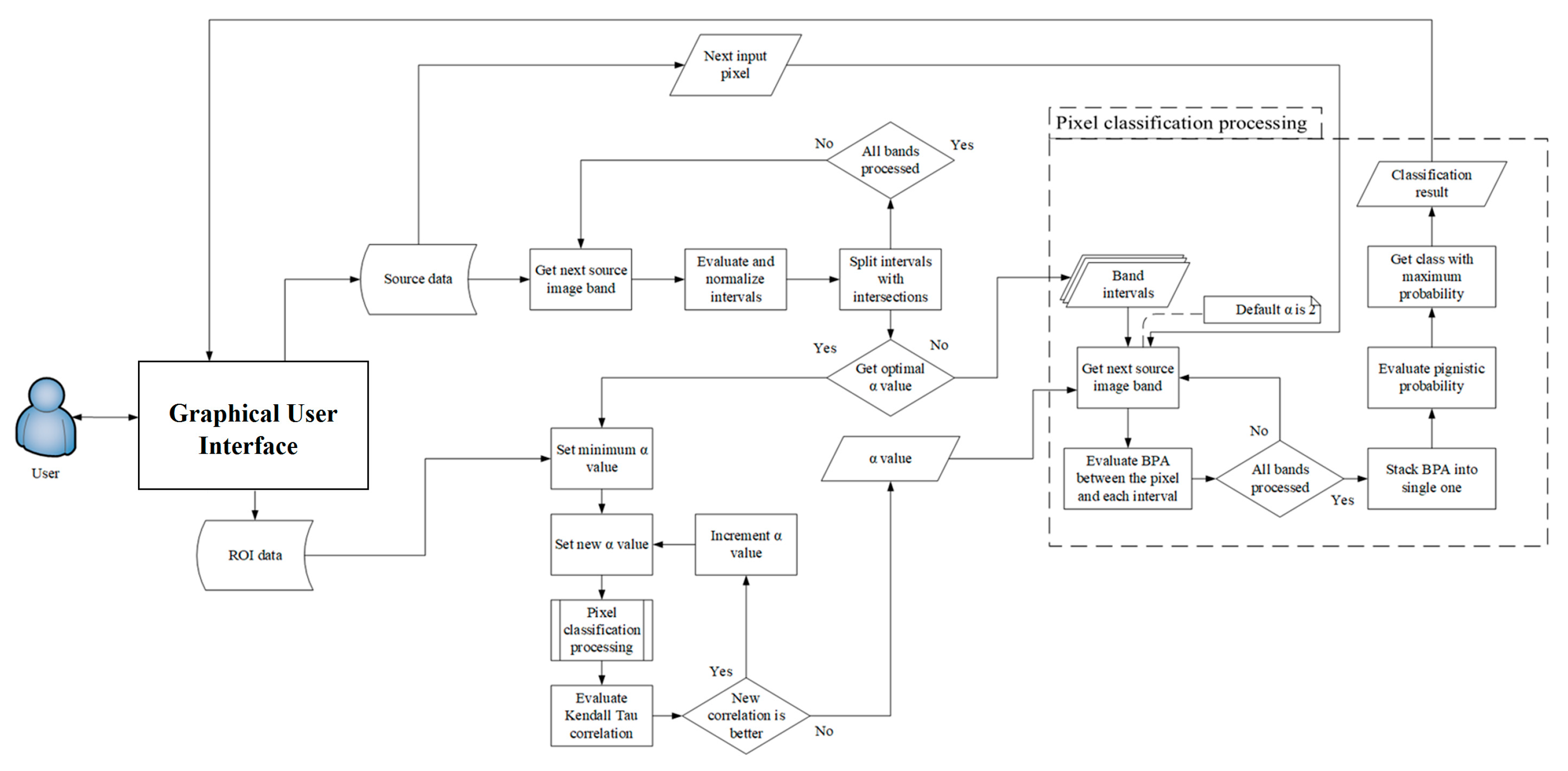
The LD assessment processing workflow follows the diagram in Figure A1.
Figure A1. LD assessment processing workflow.
Sustainability 18 06681 g0a1
The above figure shows a processing workflow depicting the internal processing of the geoinformation tool for land degradation assessment, which is hidden behind the graphical user interface (GUI).
A demonstration of the GUI of the developed geoinformation tool for land degradation assessment is shown in Figure A2.
Figure A2. Land degradation classification software simple GUI demonstration.
Sustainability 18 06681 g0a2

References

  1. Olsson, L.; Barbosa, H.; Bhadwal, S.; Cowie, A.; Delusca, K.; Flores-Renteria, D.; Hermans, K.; Jobbágy, E.; Kurz, W.; Li, D.; et al. Land Degradation. In Climate Change and Land: An IPCC Special Report on Climate Change, Desertification, Land Degradation, Sustainable Land Management, Food Security, and Greenhouse Gas Fluxes in Terrestrial Ecosystems; Shukla, P.R., Ed.; Intergovernmental Panel on Climate Change: Geneva, Switzerland, 2019; Available online: https://www.ipcc.ch/srccl/chapter/chapter-4/ (accessed on 22 September 2025).
  2. Intergovernmental Panel on Climate Change. Climate Change and Land; Cambridge University Press: Cambridge, UK, 2022. [Google Scholar] [CrossRef]
  3. United Nations Convention to Combat Desertification. Global Land Outlook; United Nations Convention to Combat Desertification: Bonn, Germany, 2017; Available online: https://www.unccd.int/sites/default/files/documents/2017-09/GLO_Full_Report_low_res.pdf (accessed on 11 June 2025).
  4. Schillaci, C.; Jones, A.; Vieira, D.; Munafò, M.; Montanarella, L. Evaluation of the United Nations Sustainable Development Goal 15.3.1 Indicator of Land Degradation in the European Union. Land Degrad. Dev. 2022, 34, 250–268. [Google Scholar] [CrossRef]
  5. Sims, N.C.; Newnham, G.J.; England, J.R.; Guerschman, J.; Cox, S.J.D.; Roxburgh, S.H.; Viscarra Rossel, R.A.; Fritz, S.; Wheeler, I. Good Practice Guidance. SDG Indicator 15.3.1, Proportion of Land That Is Degraded Over Total Land Area. Version 2.0; United Nations Convention to Combat Desertification: Bonn, Germany, 2021; Available online: https://www.unccd.int/sites/default/files/documents/2021-09/UNCCD_GPG_SDG-Indicator-15.3.1_version2_2021.pdf (accessed on 9 July 2025).
  6. Stankevich, S.A.; Kharytonov, N.N.; Dudar, T.V.; Kozlova, A.A. Risk Assessment of Land Degradation Using Satellite Imagery and Geospatial Modelling in Ukraine. In Land Degradation and Desertification—A Global Crisis; IntechOpen: London, UK, 2016. [Google Scholar] [CrossRef] [PubMed]
  7. Mountrakis, G.; Im, J.; Ogole, C. Support vector machines in remote sensing: A review. ISPRS J. Photogramm. Remote Sens. 2011, 66, 247–259. [Google Scholar] [CrossRef]
  8. United Nations Convention to Combat Desertification. The Future Strategic Framework of the Convention; Document ICCD/COP(13)/L.18; United Nations: New York, NY, USA, 2017; Available online: https://documents-dds-ny.un.org/doc/UNDOC/LTD/G17/267/81/PDF/G1726781.pdf (accessed on 11 June 2025).
  9. United Nations Office for Disaster Risk Reduction. Terminology on Disaster Risk Reduction; United Nations Office for Disaster Risk Reduction: Geneva, Switzerland, 2022; Available online: https://www.undrr.org/terminology (accessed on 11 June 2025).
  10. Van Ginkel, M.; Biradar, C. Drought Early Warning in Agri-Food Systems. Climate 2021, 9, 134. [Google Scholar] [CrossRef]
  11. Graw, V.; Dubovyk, O.; Duguru, M.; Heid, P.; Gohar, G.; Carlos, J.; Post, J.; Szarzynski, J.; Tsegai, D.; Walz, Y. Assessment, monitoring, and early warning of droughts: The potential for satellite remote sensing and beyond. Curr. Dir. Water Scarcity Res. 2019, 2, 115–131. [Google Scholar] [CrossRef]
  12. Guzzetti, F.; Gariano, S.L.; Peruccacci, S.; Brunetti, M.T.; Marchesini, I.; Rossi, M.; Melillo, M. Geographical landslide early warning systems. Earth-Sci. Rev. 2020, 200, 102973. [Google Scholar] [CrossRef]
  13. Corrado, R.; Cherubini, A.M.; Pennetta, C. Early warning signals of desertification transitions in semiarid ecosystems. Phys. Rev. E 2014, 90, 062705. [Google Scholar] [CrossRef] [PubMed]
  14. United Nations. Transforming Our World: The 2030 Agenda for Sustainable Development; United Nations: New York, NY, USA, 2015; Available online: https://sustainabledevelopment.un.org/content/documents/21252030%20Agenda%20for%20Sustainable%20Development%20web.pdf (accessed on 11 June 2025).
  15. Barger, N.; Gardner, T.A.; Sankaran, M.; Belnap, J.; Broadhurst, L.; Brochier, V.; Isbell, F.; Meyfroidt, P.; Moreira, F.; Nieminen, T.M.; et al. Chapter 3: Direct and Indirect Drivers of Land Degradation and Restoration. In The IPBES Assessment Report on Land Degradation and Restoration; Montanarella, L., Scholes, R., Brainich, A., Eds.; Intergovernmental Science-Policy Platform on Biodiversity and Ecosystem Services: Bonn, Germany, 2018; pp. 198–314. Available online: http://hdl.handle.net/2078.1/207386 (accessed on 11 June 2025).
  16. Berdimbetov, T.; Ma, Z.-G.; Shelton, S.; Ilyas, S.; Nietullaeva, S. Identifying Land Degradation and its Driving Factors in the Aral Sea Basin From 1982 to 2015. Front. Earth Sci. 2021, 9, 690000. [Google Scholar] [CrossRef]
  17. Douglas, I. The Local Drivers of Land Degradation in South-East Asia. Geogr. Res. 2006, 44, 123–134. [Google Scholar] [CrossRef]
  18. Jiang, L.; Jiapaer, G.; Bao, A.; Li, Y.; Guo, H.; Zheng, G.; Chen, T.; De Maeyer, P. Assessing land degradation and quantifying its drivers in the Amudarya River delta. Ecol. Indic. 2019, 107, 105595. [Google Scholar] [CrossRef]
  19. Karimian, H.; Zou, W.; Chen, Y.; Xia, J.; Wang, Z. Landscape ecological risk assessment and driving factor analysis in Dongjiang river watershed. Chemosphere 2022, 307, 35835. [Google Scholar] [CrossRef] [PubMed]
  20. Mirzabaev, A.; Nkonya, E.; Goedecke, J.; Johnson, T.; Anderson, W. Global Drivers of Land Degradation and Improvement. In Economics of Land Degradation and Improvement—A Global Assessment for Sustainable Development; Springer: Cham, Switzerland, 2015; pp. 167–195. [Google Scholar] [CrossRef]
  21. Perović, V.; Kadović, R.; Đurđević, V.; Pavlović, D.; Pavlović, M.; Čakmak, D.; Mitrović, M.; Pavlović, P. Major drivers of land degradation risk in Western Serbia: Current trends and future scenarios. Ecol. Indic. 2021, 123, 107377. [Google Scholar] [CrossRef]
  22. Turrini, T.; Knop, E. A landscape ecology approach identifies important drivers of urban biodiversity. Glob. Change Biol. 2015, 21, 1652–1667. [Google Scholar] [CrossRef] [PubMed]
  23. Kosmas, C.; Kairis, O.; Karavitis, C.; Ritsema, C.; Salvati, L.; Acikalin, S.; Alcala, M.; Alfama, P.; Atlhopheng, J.; Barrera, J.; et al. Evaluation and selection of indicators for land degradation and desertification monitoring: Methodological approach. Environ. Manag. 2014, 54, 951–970. [Google Scholar] [CrossRef] [PubMed]
  24. Bai, Z.G.; Dent, D.L.; Olsson, L.; Schaepman, M.E. Global Assessment of Land Degradation and Improvement. 1. Identification by Remote Sensing; Report 2008/01 (GLADA Report 5); ISRIC—World Soil Information: Wageningen, The Netherlands, 2008; Available online: https://files.isric.org/public/documents/isric_report_2008_01.pdf (accessed on 16 June 2025).
  25. Bai, Z.G.; Dent, D.L.; Olsson, L.; Schaepman, M.E. Proxy global assessment of land degradation. Soil Use Manag. 2008, 24, 223–234. [Google Scholar] [CrossRef]
  26. Jiang, K.A.; Teuling, J.; Chen, X.; Huang, N.; Wang, J.; Zhang, Z.; Gao, R.; Men, J.; Zhang, Z.; Wu, Y.; et al. Global land degradation hotspots based on multiple methods and indicators. Ecol. Indic. 2024, 158, 111462. [Google Scholar] [CrossRef]
  27. Rangel-Peraza, J.G.A.; Sanhouse-García, J.; Flores-González, L.M.; Monjardín-Armenta, S.A.; Mora-Félix, Z.D.; Rentería-Guevara, S.A.; Bustos-Terrones, Y.A. Effect of land use and land cover changes on land surface warming in an intensive agricultural region. J. Environ. Manag. 2024, 371, 123249. [Google Scholar] [CrossRef] [PubMed]
  28. Sivakumar, M.V.K.; Ndiang’ui, N. Climate and Land Degradation; Springer: Berlin/Heidelberg, Germany, 2007. [Google Scholar] [CrossRef]
  29. Higginbottom, T.; Symeonakis, E. Assessing Land Degradation and Desertification Using Vegetation Index Data: Current Frameworks and Future Directions. Remote Sens. 2014, 6, 9552–9575. [Google Scholar] [CrossRef]
  30. Kumar, B.; Babu, K.; Anusha, B.N.; Rajasekhar, M. Geo-environmental monitoring and assessment of land degradation and desertification in the semi-arid regions using Landsat 8 OLI / TIRS, LST, and NDVI approach. Environ. Chall. 2022, 8, 100578. [Google Scholar] [CrossRef]
  31. El Haj Tahir, M.; Kääb, A.; Xu, C.-Y. Identification and mapping of soil erosion areas in the Blue Nile, Eastern Sudan using multispectral ASTER and MODIS satellite data and the SRTM elevation model. Hydrol. Earth Syst. Sci. 2010, 14, 1167–1178. [Google Scholar] [CrossRef]
  32. Giuliani, G.; Chatenoux, B.; Benvenuti, A.; Lacroix, P.; Santoro, M.; Mazzetti, P. Monitoring land degradation at national level using satellite Earth Observation time-series data to support SDG15—Exploring the potential of data cube. Big Earth Data 2020, 4, 3–22. [Google Scholar] [CrossRef]
  33. AbdelRahman, M.A.E. An overview of land degradation, desertification and sustainable land management using GIS and remote sensing applications. Rend. Lincei Sci. Fis. Nat. 2023, 34, 767–808. [Google Scholar] [CrossRef]
  34. Boroughani, M.; Mirchooli, F.; Hadavifar, M.; Fiedler, S. Mapping land degradation risk due to land susceptibility to dust emission and water erosion. SOIL 2023, 9, 411–423. [Google Scholar] [CrossRef]
  35. Dwivedi, R.S. Geospatial Technologies for Land Degradation Assessment and Management; CRC Press: Boca Raton, FL, USA, 2018. [Google Scholar] [CrossRef]
  36. Ambarwulan, W.; Nahib, I.; Widiatmaka, W.; Suryanta, J.; Munajati, S.L.; Suwarno, Y.; Turmudi, T.; Darmawan, M.; Sutrisno, D. Using Geographic Information Systems and the Analytical Hierarchy Process for Delineating Erosion-Induced Land Degradation in the Middle Citarum Sub-Watershed, Indonesia. Front. Environ. Sci. 2021, 9, 710570. [Google Scholar] [CrossRef]
  37. Li, K.; Wang, J. A multi-source data fusion method for land cover production: A case study of the East European Plain. Int. J. Digit. Earth 2024, 17, 2339360. [Google Scholar] [CrossRef]
  38. Coţolan, L.; Moldovan, D. Applicability of pre-trained CNNs in temperate deforestation detection. Eur. J. Remote Sens. 2024, 57, 2367221. [Google Scholar] [CrossRef]
  39. Popov, M.; Stankevich, S.; Kozlova, A.; Piestova, I.; Lubskiy, M.; Titarenko, O.; Svideniuk, M.; Andreiev, A.; Lysenko, A.; Singh, S.K. Long-Term Satellite Data Time Series Analysis for Land Degradation Mapping to Support Sustainable Land Management in Ukraine. In Geo-Intelligence for Sustainable Development; Advances in Geographical and Environmental Sciences; Springer: Singapore, 2021; pp. 165–189. [Google Scholar] [CrossRef] [PubMed]
  40. Prăvălie, R.; Borrelli, P.; Panagos, P.; Ballabio, C.; Lugato, E.; Chappell, A.; Miguez-Macho, G.; Maggi, F.; Peng, J.; Niculiță, M. A unifying modelling of multiple land degradation pathways in Europe. Nat. Commun. 2024, 15, 3862. [Google Scholar] [CrossRef] [PubMed]
  41. Yelistratova, L.; Apostolov, A.; Khodorovskyi, A.; Tymchyshyn, M. Land cover degradation challenges in Ukraine: Natural drivers and processes. In Proceedings of the 24th International Multidisciplinary Scientific Geoconference Informatics, Geoinformatics and Remote Sensing, Albena, Bulgaria, 1–7 July 2024; pp. 265–274. [Google Scholar] [CrossRef]
  42. Yelistratova, L.; Apostolov, A.; Khodorovskyi, A.; Tymchyshyn, M. Satellite monitoring of anthropogenic processes and factors of land degradation in Ukraine. In Proceedings of the 24th International Multidisciplinary Scientific Geoconference Informatics, Geoinformatics and Remote Sensing, Albena, Bulgaria, 1–7 July 2024; pp. 295–304. [Google Scholar] [CrossRef]
  43. Bojórquez-Tapia, L.A.; Cruz-Bello, G.M.; Luna-González, L. Connotative land degradation mapping: A knowledge-based approach to land degradation assessment. Environ. Model. Softw. 2013, 40, 51–64. [Google Scholar] [CrossRef]
  44. Popov, M.; Stankevich, S.; Kozlova, A.; Piestova, I.; Khyzhnyak, A.; Zaitseva, E.; Levashenko, V.; Seredinin, E.; Maltsev, S.; Lypska, Y. The Architecture of Land Degradation Early Warning Based on Earth Observation. In Proceedings of the International Conference on Information and Digital Technology (IDT), Zilina, Slovakia, 20–22 June 2023; pp. 125–132. [Google Scholar] [CrossRef]
  45. Lehmann, A.; Mazzetti, P.; Santoro, M.; Nativi, S.; Masò, J.; Serral, I.; Spengler, D.; Niamir, A.; Lacroix, P.; Ambrosone, M. Essential earth observation variables for high-level multi-scale indicators and policies. Environ. Sci. Policy 2022, 131, 105–117. [Google Scholar] [CrossRef]
  46. Sudmanns, M.; Giuliani, G.; Tiede, D.; Augustin, H. Emerging trends in big Earth data management and analysis. Big Earth Data 2023, 7, 451–454. [Google Scholar] [CrossRef]
  47. Montero, D.; Kraemer, G.; Anghelea, A.; Aybar, C.; Brandt, G.; Camps-Valls, G.; Cremer, F.; Flik, I.; Fabian, G.; Habershon, S.; et al. Earth System Data Cubes: Avenues for advancing Earth system research. Environ. Data Sci. 2024, 3, e27. [Google Scholar] [CrossRef]
  48. Abatzoglou, J.T.; Dobrowski, S.Z.; Parks, S.A.; Hegewisch, K.C. TerraClimate, a high-resolution global dataset of monthly climate and climatic water balance from 1958–2015. Sci. Data 2018, 5, 170191. [Google Scholar] [CrossRef] [PubMed]
  49. Farr, T.G.; Rosen, P.A.; Caro, E.; Crippen, R.; Duren, R.; Hensley, S.; Kobrick, M.; Paller, M.; Rodriguez, E.; Roth, L.; et al. The Shuttle Radar Topography Mission. Rev. Geophys. 2007, 45, RG2004. [Google Scholar] [CrossRef]
  50. Sobrino, J.A.; Jimenez-Munoz, J.C.; Soria, G.; Romaguera, M.; Guanter, L.; Moreno, J.; Plaza, A.; Martinez, P. Land Surface Emissivity Retrieval From Different VNIR and TIR Sensors. IEEE Trans. Geosci. Remote Sens. 2008, 46, 316–327. [Google Scholar] [CrossRef]
  51. Brown, C.F.; Brumby, S.P.; Guzder-Williams, B.; Birch, T.; Hyde, S.B.; Mazzariello, J.; Czerwinski, W.; Pasquarella, V.J.; Haertel, R.; Ilyushchenko, S.; et al. Dynamic World, Near real-time global 10 m land use land cover mapping. Sci. Data 2022, 9, 251. [Google Scholar] [CrossRef]
  52. Leal, J.E. AHP-Express: A Simplified Version of the Analytical Hierarchy Process Method. MethodsX 2020, 7, 100748. [Google Scholar] [CrossRef] [PubMed]
  53. Chebbi, W.; Rubio, E.; García-Morote, F.A.; Andrés-Abellán, M.; Picazo-Córdoba, M.I.; Arquero-Escañuela, R.; López-Serrano, F.R. Evaluation of the Sentinel-3A Gross Dry Matter Productivity (GDMP) product for evergreen forests. In Proceedings of the EGU General Assembly 2024, Vienna, Austria, 14–19 April 2024. EGU24-12680. [Google Scholar] [CrossRef]
  54. Popov, M.A. Methodology of Accuracy Assessment of Classification of Objects on Space Images. J. Autom. Inf. Sci. 2007, 39, 48–55. [Google Scholar]
  55. Verde, R.; Irpino, A. A New Interval Data Distance Based on the Wasserstein Metric. In Data Analysis, Machine Learning and Applications; Studies in Classification, Data Analysis, and Knowledge Organization; Springer: Berlin/Heidelberg, Germany, 2008; pp. 705–712. [Google Scholar] [CrossRef]
  56. Theodoridis, S.; Koutroumbas, K. Pattern Recognition, 2nd ed.; Academic Press: San Diego, CA, USA, 2003. [Google Scholar]
  57. Huynh, V.-N. Discounting and Combination Scheme in Evidence Theory for Dealing with Conflict in Information Fusion. In Modeling Decisions for Artificial Intelligence; Torra, V., Narukawa, Y., Inuiguchi, M., Eds.; Lecture Notes in Computer Science; Springer: Berlin/Heidelberg, Germany, 2009; Volume 5861, pp. 217–230. [Google Scholar] [CrossRef]
  58. Campbell, J.B.; Wynne, R.H.; Thomas, V.A. Introduction to Remote Sensing, 6th ed.; Guilford Press: New York, NY, USA, 2023. [Google Scholar]
  59. Derryberry, D.R.; Schou, S.B.; Conover, W.J. Teaching Rank-Based Tests by Emphasizing Structural Similarities to Corresponding Parametric Tests. J. Stat. Educ. 2010, 18, 1–19. [Google Scholar] [CrossRef]
  60. Kendall, M.G.; Gibbons, J.D. Rank Correlation Methods, 5th ed.; Oxford University Press: New York, NY, USA, 1990. [Google Scholar]
  61. Gonzalez-Roglich, M.; Zvoleff, A.; Noon, M.; Liniger, H.; Fleiner, R.; Harari, N.; Garcia, C. Synergizing global tools to monitor progress towards land degradation neutrality: Trends.Earth and the World Overview of Conservation Approaches and Technologies sustainable land management database. Environ. Sci. Policy 2019, 93, 34–42. [Google Scholar] [CrossRef]
  62. Bonett, D.G.; Wright, T.A. Sample Size Requirements for Estimating Pearson, Kendall and Spearman Correlations. Psychometrika 2000, 65, 23–28. [Google Scholar] [CrossRef]
  63. Tuğran, E.; Kocak, M.; Mirtagioğlu, H.; Yiğit, S.; Mendes, M.A. Simulation Based Comparison of Correlation Coefficients with Regard to Type I Error Rate and Power. J. Data Anal. Inf. Process. 2015, 3, 87–101. [Google Scholar] [CrossRef]
  64. Wickramarathne, T.L.; Premaratne, K.; Murthi, M.N. Toward Efficient Computation of the Dempster–Shafer Belief Theoretic Conditionals. IEEE Trans. Cybern. 2013, 43, 712–724. [Google Scholar] [CrossRef] [PubMed]
  65. Kaltsounidis, A.; Karali, I. Dempster-Shafer Theory: How Constraint Programming Can Help. In Information Processing and Management of Uncertainty in Knowledge-Based Systems; Lesot, M.-J., Vieira, S.M., Reformat, M.Z., Carvalho, J.P., Wilbik, A., Bouchon-Meunier, B., Yager, R.R., Eds.; Communications in Computer and Information Science; Springer: Cham, Switzerland, 2020; Volume 1237, pp. 354–367. [Google Scholar] [CrossRef]
  66. Stankevich, S.; Kozlova, A.; Piestova, I.; Sedlerova, O.; Lubskyi, M.; Andreiev, A.; Orlenko, T.; Ibouh, H.; Mezzane, D.; Aboufirass, M.; et al. Earth observation-based land degradation mapping and prediction: The Moroccan test region case study. IEEE J. Sel. Top. Appl. Earth Obs. Remote Sens. 2026, 19, 11361–11377. [Google Scholar] [CrossRef]
  67. Hüllermeier, E. Similarity-based inference as evidential reasoning. Int. J. Approx. Reason. 2001, 26, 67–100. [Google Scholar] [CrossRef]
  68. Yager, R.R. Comparing approximate reasoning and probabilistic reasoning using the Dempster–Shafer framework. Int. J. Approx. Reason. 2009, 50, 812–821. [Google Scholar] [CrossRef][Green Version]
Figure 1. Location of the study area.
Sustainability 18 06681 g001
Figure 2. LD mapping general flowchart.
Sustainability 18 06681 g002
Figure 3. Interval-valued number displacement based on the temperature source data.
Sustainability 18 06681 g003
Figure 4. Sensitivity of Kendall’s τ to parameter α: (a) whole plot with blue dots indicating the plot values; (b) zoomed fragment with highlighted current α = 1.935 value.
Sustainability 18 06681 g004
Figure 5. Ablation analysis of Kendall’s τ response to indicator discarding.
Sustainability 18 06681 g005
Figure 6. Land degradation classification map over the study area. Sustainability 18 06681 i001—high degradation, Sustainability 18 06681 i002—low degradation, Sustainability 18 06681 i003—neutral condition, Sustainability 18 06681 i004—land remediation.
Sustainability 18 06681 g006
Figure 7. Interval number displacement according to the LD indicators (image bands).
Sustainability 18 06681 g007
Figure 8. Distribution of the sampling points within the study area.
Sustainability 18 06681 g008
Figure 9. LD mapping within the study area: (a)—evidence-based (ours), (b)—SVM classification, (c)—SDG Indicator 15.3.1 using Trends.Earth methodology. Sustainability 18 06681 i008—high degradation, Sustainability 18 06681 i009—low degradation, Sustainability 18 06681 i010—neutral condition, Sustainability 18 06681 i011—land remediation.
Sustainability 18 06681 g009
Table 1. LULC class transition rules for SDG Indicator 15.3.1 estimation: Sustainability 18 06681 i005—degradation, Sustainability 18 06681 i006—neutral condition, Sustainability 18 06681 i007—land remediation.
Tree-CoveredGrasslandCroplandWetlandArtificialBare LandWater
Tree-Covered
Grassland
Cropland
Wetland
Artificial
Bare Land
Water
Table 2. Accuracy assessment metrics for the control points in the LD mapping area.
LD Mapping TechniqueKendall’s Correlation CoefficientConfidence IntervalIoUOAKappa
Evidence-based (presented)0.832[0.703, 0.908]1.00.8250.767
SVM classification0.806[0.66, 0.893]0.7690.80.733
Trends.Earth0.462[0.175, 0.676]0.00.4250.052
Disclaimer/Publisher’s Note: The statements, opinions and data contained in all publications are solely those of the individual author(s) and contributor(s) and not of MDPI and/or the editor(s). MDPI and/or the editor(s) disclaim responsibility for any injury to people or property resulting from any ideas, methods, instructions or products referred to in the content.