Article

Sustainability-Oriented Governance of Tourism Corridors: Decoupling Socioeconomic Pressure and Ecological Vulnerability with Explainable AI and Evolutionary Optimization

1
School of Architecture and Planning, Jilin University of Architecture and Technology, Changchun 130114, China
2
School of Architecture and Spatial Planning, Anhui Jianzhu University, Hefei 230009, China
3
Shenzhen Tourism College, Jinan University, Shenzhen 518053, China
4
School of Innovation and Creation Design, Shenzhen Polytechnic University, Shenzhen 518053, China
5
School of Architecture, Harbin Institute of Technology, Shenzhen 518055, China
*
Authors to whom correspondence should be addressed.
Sustainability 2026, 18(13), 6631; https://doi.org/10.3390/su18136631
Submission received: 28 May 2026 / Revised: 26 June 2026 / Accepted: 28 June 2026 / Published: 30 June 2026

Abstract

Linear tourism corridors can stimulate regional economic revitalization, but they may also intensify land conversion, fragment habitats, and challenge the long-term sustainability of ecologically sensitive landscapes. Resolving this tension requires a transition from qualitative zoning to data-driven, threshold-informed spatial governance. This study develops a continuous analytical pipeline to support land-use governance along China National Highway 331 (G331). We integrated principal component analysis (PCA) with a Bayesian-optimized eXtreme Gradient Boosting (XGBoost) model, validated through Spatial Block Cross-Validation to reduce spatial data leakage and provide a more conservative assessment of geographic transferability. Shapley Additive Explanations (SHAP) was used to interpret localized non-linear associations, threshold patterns, and spatially heterogeneous model responses. Empirical results indicate that anthropogenic socioeconomic intensity is the dominant predictive driver associated with spatial variation in ecological quality. The SHAP analysis identified model-derived threshold patterns, including an approximate population-density threshold around 4000 people per square kilometer and a corridor-distance response around 50 km from the G331 highway. To translate these model-derived explanatory insights into spatial governance scenarios, the Non-dominated Sorting Genetic Algorithm II (NSGA-II) was used to approximate the Pareto trade-off frontier between ecological integrity and socioeconomic expansion. This multi-objective optimization delineated three spatial governance scenarios and identified a Pareto-elbow configuration that supports compatible-use management. This closed-loop framework provides a transferable analytical approach for sustainability-oriented corridor governance by identifying where development may be concentrated, where ecological buffers should be strengthened, and where strict conservation should be prioritized.

1. Introduction

Tourism development has become an important driver of regional economic revitalization, yet its expansion often intensifies land conversion, ecological disturbance, and pressure on fragile landscapes [1,2]. In regions where ecological assets and human activities coexist within limited spatial ranges, tourism planning must address not only growth generation but also the long-term sustainability of the coupled social–ecological system [3,4]. This challenge is especially evident along linear transport corridors, where roads reorganize accessibility, concentrate development, and reshape spatial interactions between economic activity and environmental quality [5]. Under such conditions, tourism corridors can function both as engines of regional development and as sources of ecological vulnerability, making their governance a central issue for sustainable land-use planning [6]. Comparable pressures have been observed in protected and ecologically sensitive tourism destinations across Europe and Asia. Plitvice Lakes National Park, Cinque Terre National Park, Maya Bay, and Sagarmatha National Park all show how rapid visitation growth, infrastructure expansion, crowding, waste discharge, and habitat disturbance can exceed local governance capacity [7,8,9,10]. These cases indicate that the central question is not whether tourism should develop, but how visitor access, infrastructure provision, and ecological carrying capacity can be spatially coordinated before degradation becomes irreversible.
This challenge is particularly acute in corridor-based tourism systems embedded in mountainous, forested, coastal, or riparian landscapes. Unlike compact urban regions or isolated destinations, linear tourism corridors exhibit strong spatial anisotropy, uneven development intensity, and localized clustering of tourism resources [11]. Improved accessibility can stimulate local economies, but without threshold-based regulation it may also accelerate habitat fragmentation, trail degradation, waste discharge, crowding pressure, and cumulative ecosystem weakening [12,13]. These trade-offs vary across space according to natural topography, socioeconomic pressure, and accessibility structure [14]. Identifying spatial thresholds and interaction mechanisms is therefore essential for designing low-impact, sustainability-oriented tourism strategies [15].
This study is theoretically grounded in social–ecological systems theory and sustainability science. From a social–ecological systems perspective, tourism corridors are not merely spatial carriers of visitor movement or infrastructure investment; they are coupled systems in which socioeconomic activities, accessibility structures, ecological vulnerability, and governance interventions interact dynamically. In this framework, tourism development represents the social and economic subsystem, ecological quality represents the environmental subsystem, and corridor accessibility functions as the spatial interface through which human pressure is transmitted to sensitive landscapes. Sustainability-oriented governance therefore requires more than evaluating whether a destination is suitable for development. It requires identifying how socioeconomic pressures and accessibility conditions reshape ecological vulnerability across space, where non-linear thresholds emerge, and how governance can redirect development toward more resilient spatial configurations.
Tourism corridor governance differs from conventional destination management in several important ways. Conventional destination management often focuses on bounded scenic areas, individual attractions, or administrative units. In contrast, corridor governance must address linearity, spatial anisotropy, cross-regional flows, and uneven pressure accumulation along transport axes. Roads, service nodes, scenic spots, riparian zones, and settlement clusters are not isolated elements; rather, they form a continuous spatial system in which local development decisions may generate cumulative ecological consequences along the corridor. As a result, the governance challenge is not only to manage tourism demand at specific sites, but also to coordinate access, land-use intensity, ecological buffers, and development nodes across a connected landscape.
Within this theoretical perspective, explainable artificial intelligence contributes not only as a technical tool but also as a conceptual bridge between complex system diagnosis and sustainability governance. Traditional planning models often translate ecological vulnerability into static suitability categories, while black-box machine learning may improve prediction without clarifying why certain areas are vulnerable or how governance should respond. By contrast, explainable AI makes the internal logic of non-linear social–ecological interactions visible. SHAP-based interpretation identifies the relative contribution of socioeconomic pressure, topographic conditions, and accessibility factors; detects thresholds at which development pressure becomes ecologically harmful; and reveals spatially differentiated mechanisms that can be translated into governance scenarios. In this sense, explainable AI functions as a knowledge-production mechanism for sustainability science: it converts complex spatial relationships into interpretable, threshold-based, and policy-relevant evidence.
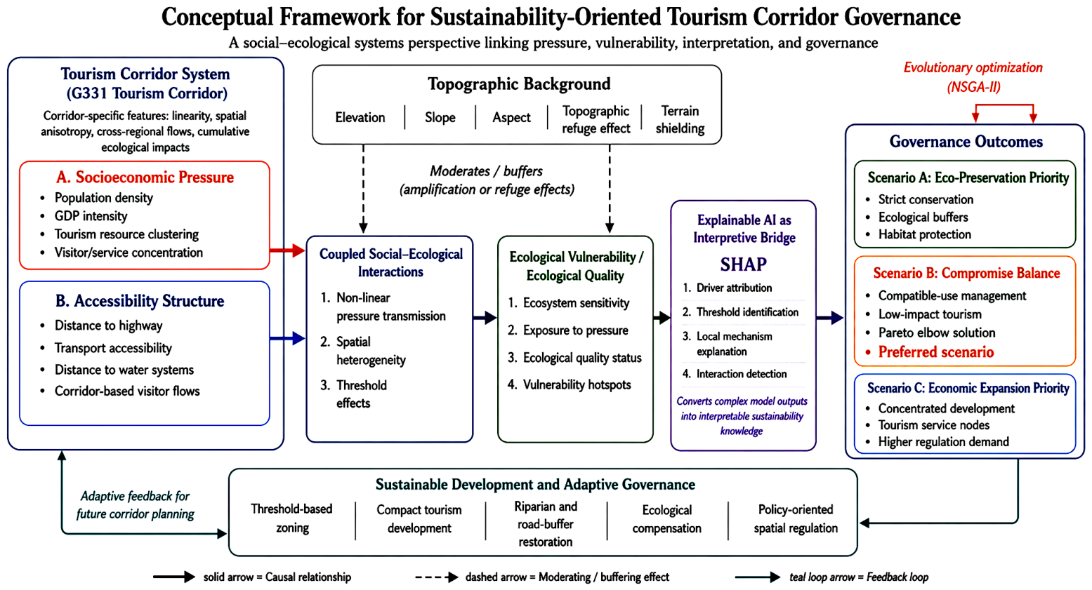
Based on this theoretical foundation, the conceptual model of this study links four components: socioeconomic pressure, ecological vulnerability, accessibility structure, and governance outcomes. Socioeconomic pressure, represented by population density and economic development intensity, reflects the human disturbance component of the tourism social–ecological system. Ecological vulnerability, represented by ecological quality and land-use-based ecological value, reflects the sensitivity and resilience of the environmental subsystem. Accessibility factors, including distance to the G331 highway and distance to water systems, mediate the spatial transmission of development pressure. Topographic conditions, including elevation, slope, and aspect, provide the physical background that may either amplify disturbance exposure or create ecological refuges. The governance outcome is expressed through threshold identification and spatial governance scenarios, including ecological preservation, compromise balance, and economic expansion pathways. Therefore, the proposed framework advances existing social–ecological systems research by transforming general concepts of coupling, resilience, and governance into a spatially explicit, explainable, and scenario-oriented model for tourism corridor sustainability (Figure 1).
Building on this conceptual framework, the following review focuses on four unresolved issues that limit the translation of sustainability theory into corridor-scale planning practice. First, many studies on sustainable tourism, protected-area management, and landscape ecological assessment still rely on composite indices, GIS-based suitability evaluation, or conventional regression models. These approaches are useful for describing spatial patterns and identifying sensitive areas, but they often depend on predefined indicator weights, assume additive or monotonic relationships, and provide limited capacity to detect non-linear ecological thresholds or interaction effects [16,17]. This limitation is particularly important for tourism corridors, where ecological vulnerability is shaped not only by the intensity of tourism development, but also by the spatial arrangement of roads, settlements, tourism resources, water systems, and ecological patches.
Second, recent studies have increasingly introduced machine learning and explainable artificial intelligence into environmental planning, ecological assessment, urban sustainability, and tourism-related decision-making [18,19,20]. These studies demonstrate that algorithms such as random forest, gradient boosting, and XGBoost can improve predictive performance when modelling complex human–environment interactions. However, many existing applications still use explainable AI mainly as a post hoc tool for feature ranking, while its role in generating sustainability-oriented planning knowledge remains insufficiently developed. In particular, SHAP-based interpretation has been widely used to identify variable importance, marginal effects, local responses, and threshold behavior, but fewer studies have connected SHAP-derived mechanisms to spatial governance, land-use regulation, or tourism-corridor scenario design [21,22,23]. Therefore, the contribution of explainable AI should not be limited to improving transparency; it can also help reveal how social–ecological vulnerability is produced, where critical thresholds emerge, and how governance responses should be spatially differentiated.
Third, previous tourism corridor studies have examined scenic-route development, accessibility improvement, tourism-resource distribution, ecological sensitivity, and land-use conflicts [24,25,26]. These studies have clarified that tourism corridors differ from conventional destinations because they are linear, cross-regional, and strongly shaped by transport axes and cumulative visitor flows. Nevertheless, much of this literature remains descriptive or diagnostic. Existing studies often identify where tourism resources, ecological risks, or land-use conflicts are located, but they provide limited evidence on how socioeconomic pressure and accessibility jointly generate ecological thresholds, how topographic conditions moderate corridor vulnerability, or how such empirical mechanisms can be translated into operational governance scenarios.
Fourth, multi-objective optimization has been increasingly applied in land-use planning, conservation prioritization, tourism development, and environmental decision-making to balance competing ecological and socioeconomic objectives [27,28,29]. Different multi-criteria decision-making and optimization methods have different strengths. Weighted-sum approaches and AHP-based evaluation are transparent and easy to implement, but they require predefined weights and often collapse multiple objectives into a single composite score. TOPSIS and related ranking methods are useful for selecting alternatives from a fixed set of scenarios, but they do not directly generate a continuous Pareto frontier. In contrast, evolutionary multi-objective algorithms such as NSGA-II are particularly suitable when planning objectives are conflicting, non-linear, and spatially constrained, because they can generate a diverse set of non-dominated solutions rather than a single weighted optimum. However, many optimization-based studies begin directly with predefined objective functions and constraints, without first explaining the social–ecological mechanisms that generate spatial vulnerability. As a result, optimization outputs may identify efficient trade-offs, but they often provide limited insight into why specific areas should be assigned to strict conservation, compatible use, or concentrated development.
Taken together, these limitations show that the central research gap is not simply a lack of predictive accuracy. The more important challenge is how to move from ecological diagnosis to spatial governance. Sustainability-oriented corridor planning requires a framework that can first disentangle correlated natural, socioeconomic, and accessibility drivers; then capture non-linear ecological responses; further explain where and why threshold-dependent vulnerability emerges; and finally translate these explanations into spatial governance scenarios. This study addresses this gap by integrating PCA, XGBoost, SHAP, Spatial Block Cross-Validation, and NSGA-II into a closed-loop analytical framework [30,31,32]. The framework links four analytical steps: driver decoupling, non-linear prediction, mechanism interpretation, and multi-objective scenario optimization.
In this framework, each method performs a specific function rather than serving as an isolated technical tool. PCA reduces multicollinearity among topographic, socioeconomic, and accessibility indicators and creates a more stable feature space. XGBoost captures non-linear ecological responses that cannot be adequately represented by linear regression or additive suitability models. Spatial Block Cross-Validation reduces the risk of spatial data leakage and provides a more conservative assessment of geographic transferability. SHAP is used not only to rank variables, but also to interpret how socioeconomic pressure, accessibility structure, and topographic background generate thresholds, local mechanisms, and interaction effects. NSGA-II then converts these diagnostic insights into Pareto-optimal spatial governance scenarios that balance ecological integrity and socioeconomic potential. In this way, the proposed framework connects explanation with planning action and transforms model outputs into interpretable governance pathways.
The novelty of this integration lies in its closed-loop structure. PCA clarifies the structure of the driving system; XGBoost models non-linear ecological vulnerability; SHAP explains why and where vulnerability emerges; and NSGA-II transforms these explanations into spatial governance scenarios. In this sense, the framework generates scientific insights beyond improved prediction accuracy. It identifies threshold-dependent ecological responses, reveals how development pressure is transmitted through corridor accessibility, clarifies the moderating role of topographic conditions, and provides a decision-oriented pathway for moving from ecological diagnosis to sustainability governance.
The empirical analysis applies this framework to the Jilin section of National Highway G331 in eastern Jilin Province, China. The corridor contains extensive forested landscapes, water-related ecosystems, topographically complex terrain, and concentrated tourism resources, making it a suitable case for examining how ecological conservation and tourism development interact within a linear accessibility system [33,34,35].
Against this background, the study addresses three questions. First, which corridor-related driver components exert the strongest influence on ecological quality, and how can their effects be disentangled in a robust and interpretable way? Second, where do key non-linear thresholds and interaction effects emerge under increasing demographic and infrastructural pressure? Third, how can these empirical insights be translated into spatial governance scenarios that support sustainable tourism development while safeguarding ecological stability?

2. Materials and Methods

2.1. Study Area

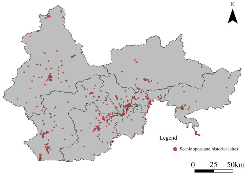
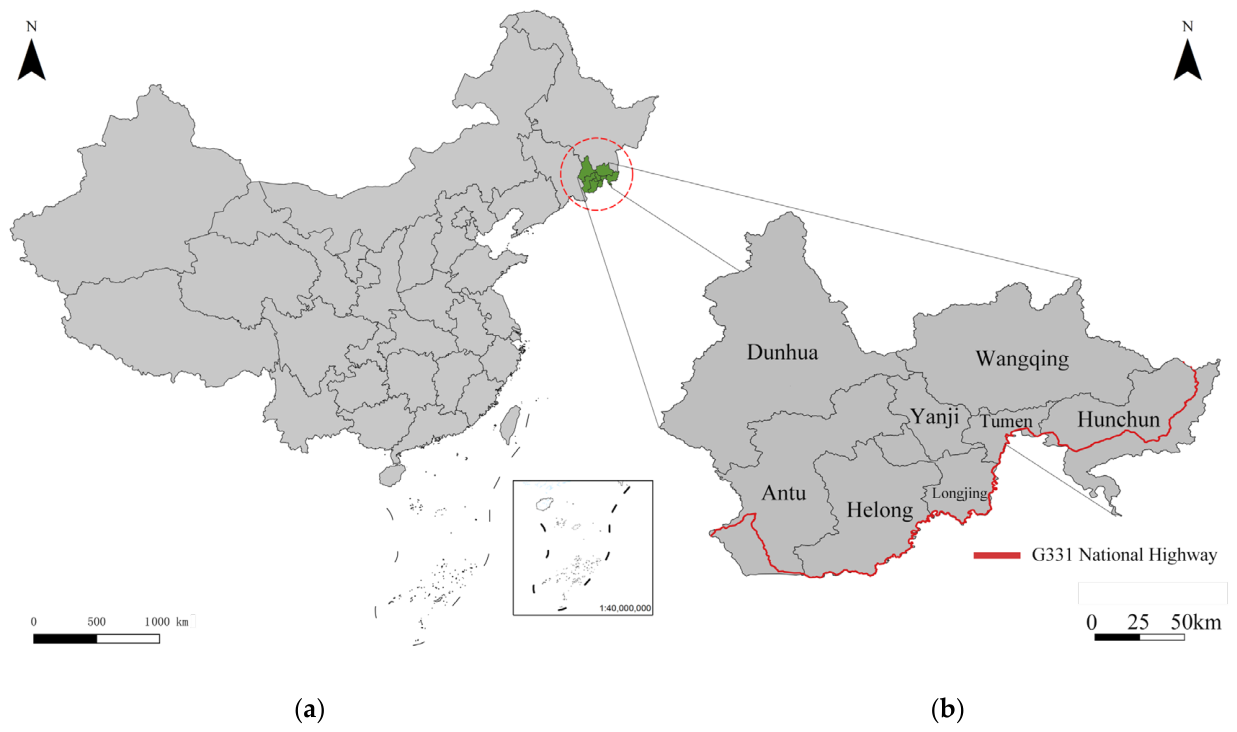
This study focuses on the G331 National Highway corridor in eastern Jilin Province, with the analytical scope consistently defined at the same administrative level throughout the manuscript. Located in the eastern part of Jilin Province, China (127°27′ E–131°18′ E, 41°59′ N–44°30′ N), the study area spans the corridor zone along the Jilin section of the G331 National Highway, covering approximately 43,300 km2 and encompassing multiple counties and cities within a highly heterogeneous mountainous landscape. As a prominent linear corridor, this region provides an ideal setting for examining the interaction between ecological conservation, accessibility, and tourism development under strong spatial constraints (Figure 2).
From a sustainability perspective, the corridor contains extensive forested and water-related ecosystems with strong conservation value, requiring tourism development to remain compatible with biodiversity protection and habitat connectivity. These ecological characteristics make the corridor a useful case for testing how development intensity can be aligned with ecological carrying capacity and long-term landscape resilience.
In terms of spatial configuration and transport infrastructure, the G331 National Highway (Jilin Section) has created new opportunities for regional resource integration. As a key linear infrastructure project, the G331 connects core counties and cities such as Hunchun, Tumen, Longjing, Helong, and Antu, forming the spatial framework of a prominent linear tourism corridor. This corridor serves as a physical carrier for 1468 tourism resources along the route and acts as a key area for the transformation of cross-regional ecological and socioeconomic flows.
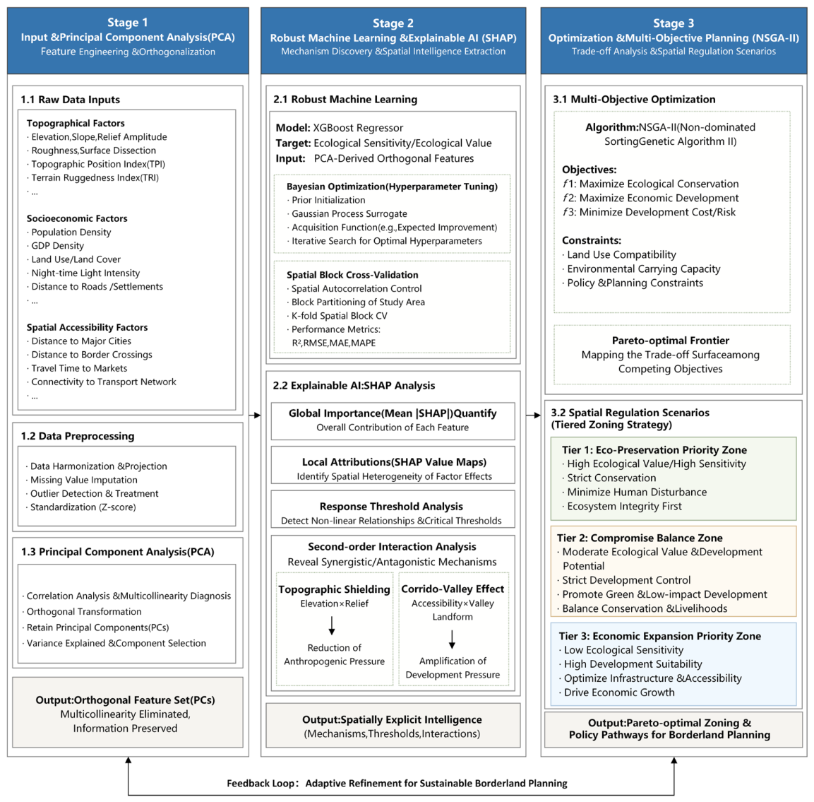
With the expansion of corridor-based tourism, the study area faces a spatial trade-off between tourism utilization and ecological conservation. Understanding the non-linear relationships that shape ecological quality is therefore essential not only for balancing socioeconomic potential and environmental protection, but also for guiding compact, low-impact, and sustainability-oriented spatial planning. To address these multidimensional trade-offs, this study uses the natural geomorphic and socioeconomic gradients of this region to construct a data-driven analytical framework. PCA, XGBoost, SHAP, Spatial Block Cross-Validation, and NSGA-II are then integrated to support ecological diagnosis, mechanism interpretation, and spatial governance scenario generation for corridor-scale planning (Figure 3).

2.2. Variable Selection and Measurement

2.2.1. Selection and Measurement of Corridor Predictors

The selection of variables was guided by three principles: theoretical relevance, spatial availability, and comparability across the entire corridor. First, the variables had to represent the main components of the tourism corridor social–ecological system, including topographic background, socioeconomic pressure, spatial accessibility, and ecological quality. Second, they had to be available as spatially continuous or consistently gridded datasets across the full G331 corridor, because the analysis required a unified 500 m × 500 m spatial framework. Third, the variables had to be comparable across counties and landscape types to avoid introducing administrative reporting bias. For this reason, the model prioritizes land-use-based ecological quality, topographic constraints, population density, GDP intensity, highway accessibility, and water-system proximity. These indicators do not capture all dimensions of tourism disturbance or biodiversity, but they provide a consistent and reproducible proxy system for evaluating corridor-scale ecological vulnerability (Table 1).
Because the available datasets were not produced in the same year or updated at the same temporal frequency, the analysis should be interpreted as a cross-sectional representation of corridor-scale spatial associations rather than a longitudinal assessment of ecological change.
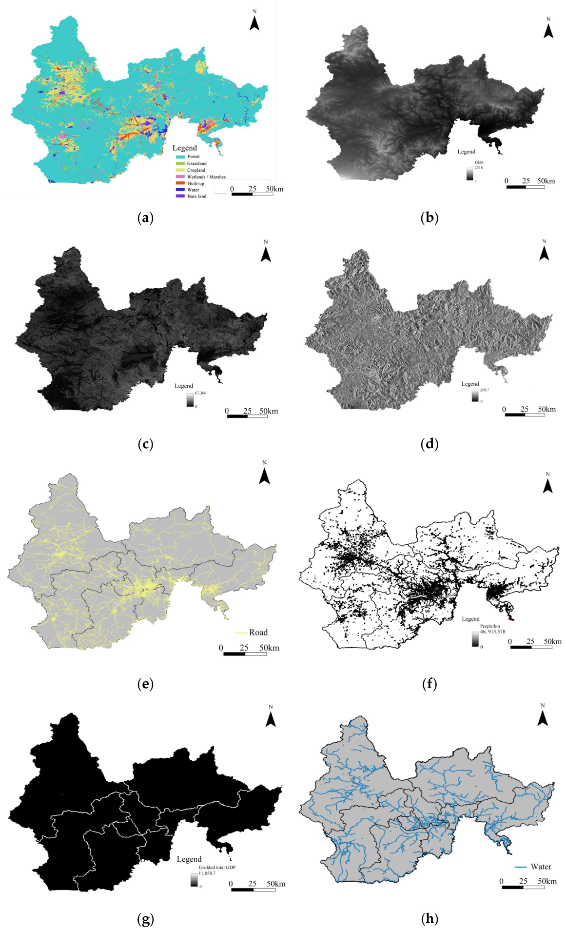
The spatial distribution patterns of each predictor variable in Yanbian Prefecture exhibit significant heterogeneity. The detailed spatial mapping is presented in Figure 4.
(1) Response variable: Ecological Quality Score (Eco_Score)
In this study, Eco_Score was selected as the dependent variable to measure the background ecological quality of tourism resource sites. This indicator was constructed based on high-resolution land use and land cover change (LUCC) data (Figure 4a). The rationale for using a land-use-based ecological quality indicator is that land cover provides a spatially explicit and consistently observable proxy for habitat integrity, ecosystem-service capacity, and the degree of human disturbance. Forests and water bodies generally indicate higher biodiversity-supporting capacity, carbon sequestration, water regulation, and habitat connectivity, whereas built-up land and degraded unused land usually reflect stronger artificial disturbance and lower ecological carrying capacity. Therefore, Eco_Score does not represent direct species-level biodiversity; rather, it represents landscape-level ecological quality and habitat-service potential.
The reliability of Eco_Score is supported by three aspects. First, it is derived from spatially continuous LUCC data, which avoids the uneven sampling problem often associated with field-based ecological or biodiversity observations. Second, the scoring matrix follows established ecosystem-service valuation and ecological contribution frameworks, while being adjusted to the ecological context of temperate forest landscapes in Northeast China. Third, the index is calculated using an area-weighted method within 500 m grid units, allowing each tourism resource site to be evaluated according to the surrounding landscape matrix rather than by a single point attribute. This makes Eco_Score suitable for corridor-scale spatial modelling, although it should be interpreted as a proxy for ecological quality rather than a comprehensive biodiversity index.
(2) Topographic Background Factors
Topographic factors constitute the physical substrate that shapes the ecological landscape of Yanbian Prefecture. In this study, elevation, slope, and aspect were selected as topographic predictors (Figure 4b–d). Elevation and slope contribute to a topographic refuge effect. While socioeconomic pressure may drive ecological degradation, high-altitude and steep-slope terrains can act as physical barriers that shield core ecological patches from human encroachment. This provides a useful basis for delineating strict conservation zones within the social–ecological systems framework. Aspect indirectly affects the microclimate and ecological sensitivity of the landscape by influencing the solar radiation received by the surface.
(3) Socioeconomic Pressure Factors
Human activities are the main disturbance sources closely associated with fluctuations in ecological quality. This study incorporates population density (Pop_Density) and economic development level (GDP) to represent the intensity of human activities (Figure 4f,g). High population density and robust economic activity often lead to increased land development intensity, a significant negative pressure that causes fragmentation and degradation of regional ecological patches.
(4) Spatial Accessibility Factors
As key spatial features of the linear tourism corridor, road accessibility and water-system proximity influence both tourism development potential and ecological sensitivity. This study calculated the distance from the G331 National Highway (Dist_G331) to represent the spatial influence of corridor accessibility on surrounding ecosystems (Figure 2b). The distance from water systems (Dist_to_Water) was also included because it reflects both the water-related attractiveness of tourism resources and the protection needs of water-related ecologically sensitive zones (Figure 4h).

2.2.2. Ecological Quality Index (EQI) Construction

To quantify corridor-scale ecological quality, this study constructed Eco_Score, a land-use-based Ecological Quality Index (EQI), as the response variable for the machine-learning model. The index uses land-use/land-cover data and an ecological contribution matrix to represent habitat integrity and ecosystem-service capacity across landscape units. Throughout the manuscript, Eco_Score refers to this operational EQI variable, whereas “ecological quality” is used as the broader conceptual term.
(1) Scoring Matrix and Weight Assignment
This study refers to the ecosystem service value (ESV) assessment framework proposed by Costanza et al. [33], and combines the modified ecological contribution coefficients for the temperate forest area in Northeast China by Xie Guojiu et al. [31,32], to establish the mapping relationship between land use types and ecological quality scores. The specific scoring logic follows the following principles:
① High-value area (0.8–1.0): Forest land and water bodies are given the highest scores. Forest land, which serves as the ecological barrier of Changbai Mountain, plays a crucial role in water conservation and biodiversity maintenance. Water bodies are essential regulators for maintaining the ecological balance of the region.
② Medium-value area (0.4–0.7): Grassland and farmland belong to the medium ecological value area. Although they have certain primary productivity, due to a certain degree of disturbance from agricultural activities, their ecological stability is lower than that of the original forest land.
③ Low-value area (0.1–0.2): Built-up land and unused land are given the lowest scores. It should be noted that ‘unused land’ in this dataset primarily refers to degraded bare land near development zones rather than high-altitude primary alpine tundra, thereby justifying its low ecological weight in this specific regional context.
The detailed ecological scoring weights for each land use type are shown in Table 2. Biodiversity indicators such as species richness, habitat occupancy, or protected-species records were not included as direct model variables for two reasons. First, such data are rarely available at a consistent spatial resolution across the entire corridor, and field-observed biodiversity records may be biased toward accessible areas, protected sites, or frequently surveyed locations. Second, the objective of this study is to model corridor-scale ecological vulnerability associated with land-use structure and development pressure, rather than to conduct species-specific biodiversity assessment. To partially account for biodiversity-related ecological functions, the EQI assigns higher values to forests and water bodies because these land-cover types generally provide stronger habitat support, landscape connectivity, and ecosystem-service capacity. Nevertheless, we acknowledge that Eco_Score cannot fully replace direct biodiversity indicators. Future research should integrate species-distribution data, habitat-quality models, remote-sensing biodiversity proxies, or field-based ecological monitoring when such data become available.
(2) Spatial Quantification and Index Calculation
Because the 1468 tourism resource sites are distributed across heterogeneous landscape backgrounds, the attributes of a single point location are insufficient to capture the ecological quality of the surrounding environment. Therefore, this study adopts the area-weighted average method to calculate the EQI within 500 m grid units. The calculation formula is as follows:
E Q I j   =   i = 1 n S i × A i , j A j
where EQIj represents the ecological quality score of the jth analysis unit; Si is the ecological weight value of the i-th type of land use; Ai,j is the area of the i-th type of land use within this unit; Aj is the total area of the unit, and n is the total number of land types.
(3) Normalization and Sensitivity Verification. To ensure numerical comparability and support stable XGBoost model training, the original Eco_Score obtained through Equation (1) was normalized to a [0, 100] scale using the Min–Max normalization method:
EQ I norm   =   EQI     EQI min EQI max     EQI min   ×   100
A higher final score indicates better landscape-level ecological quality and lower relative disturbance, rather than a direct indication of suitability for intensive human development. This quantitative process converts the qualitative landscape classification into quantitative continuous variables, laying a data foundation for analyzing the non-linear associations of environmental factors. To examine whether the model results were affected by the ecological weighting scheme used to construct Eco_Score, we conducted a sensitivity analysis using two alternative dominant-land-use-based weighting schemes. The conservative scheme reduced the contrast between high-ecological-value and medium-ecological-value land-use categories, whereas the disturbance-sensitive scheme imposed stronger penalties on built-up and unused land. The results indicate that the absolute Eco_Score values were moderately sensitive to weighting assumptions. Compared with the baseline Eco_Score, the conservative scheme produced a Pearson correlation of 0.795 and a Spearman correlation of 0.499, while the disturbance-sensitive scheme produced a Pearson correlation of 0.750 and a Spearman correlation of 0.505. However, the main predictive structure of the PCA-XGBoost-SHAP model remained broadly stable. The mean cross-validated R2 values were 0.917, 0.888, and 0.876 under the baseline, conservative, and disturbance-sensitive schemes, respectively. In all three models, PC1 remained the most important SHAP component, followed by PC2. These results suggest that the main model-based interpretation is not solely an artifact of a single ecological weighting assumption, although the absolute Eco_Score values should be interpreted with caution. The detailed comparison of alternative Eco_Score weighting schemes is reported in Appendix A Table A1.

2.2.3. Data Integration and Spatial Feature Extraction

After establishing a multidimensional predictor system composed of topographic background, socioeconomic pressure, and spatial accessibility, this subsection explains how Geographic Information System (GIS) techniques were used to integrate multi-source and cross-scale datasets into a standardized spatial feature matrix suitable for machine-learning modelling. This process not only involves geometric alignment in physical space but also includes the extraction of key features of the spatial clustering intensity of tourism resource points (POI: Point of Interest).
(1) Quantification of the spatial clustering of tourism resource points (POIs)
The 1468 tourism resource points obtained in this study exhibit a significant spatially non-uniform distribution pattern, as shown in Figure 5. Statistical data indicate that there are 312 (21.25%) in Antu County, 296 (20.16%) in Dunhua City, 267 (18.19%) in Helong City, 195 (13.28%) in Yanji City, 136 (9.26%) in Tumen City, 109 (7.43%) in Longjing City, 80 (5.45%) in Hunchun City, and 73 (4.97%) in Wangqing County, which constitute the core carrying area of tourism in Yanbian.
To depict the spatial clustering of tourism resources, this study employed Kernel Density Estimation (KDE) to perform spatial smoothing on the POIs.
① Calculation logic: The search radius was set at 5 km. By estimating the concentration of tourism resource points within each unit area, a continuous spatial density surface was generated.
② Feature identification: The results show that the tourism resources in Yanbian exhibit a “central concentration and linear dispersion” pattern, forming a spatial layout with the central urban area of Yanji as the primary core, and Dunhua and Antu as secondary cores. This provides a macroscopic geographical background for understanding the spatial aggregation of tourism resources. Consequently, POI density is used strictly for contextual spatial mapping, while socioeconomic indicators, including GDP intensity and population density, serve as direct quantitative proxies for human disturbance in the machine-learning models. Tourism-intensity indicators such as visitor flows, accommodation density, tourism revenue, and seasonal tourism pressure were not included as direct explanatory variables because consistent, fine-scale, and corridor-wide datasets were not available for all tourism resource sites. In particular, visitor-flow data are often reported at the level of individual scenic areas or administrative units, while accommodation statistics and tourism revenue are usually aggregated by county or city and may not correspond to the spatial unit of ecological exposure. Directly integrating such heterogeneous data could introduce scale mismatch, reporting bias, and endogeneity, because high tourism revenue or accommodation density may be both a cause and an outcome of accessibility and local development intensity. Therefore, this study uses population density, GDP intensity, distance to the G331 highway, distance to water systems, and POI density mapping to represent the broader spatial conditions under which tourism-related human pressure is generated. However, we agree that visitor flows, accommodation density, tourism revenue, and seasonal pressure could provide additional explanatory power if spatially harmonized data are available. These variables should be incorporated into future dynamic models to better capture temporal tourism disturbance.
(2) Spatial alignment and resampling of multi-scale data. Due to differences in the original spatial resolutions of terrain factors (30 m), socioeconomic factors (100 m–1 km), and POI density data, this study established a unified geographic calculation benchmark:
① Unified coordinate system. All data are reprojected to WGS 84/UTM zone 52N (EPSG:32652).
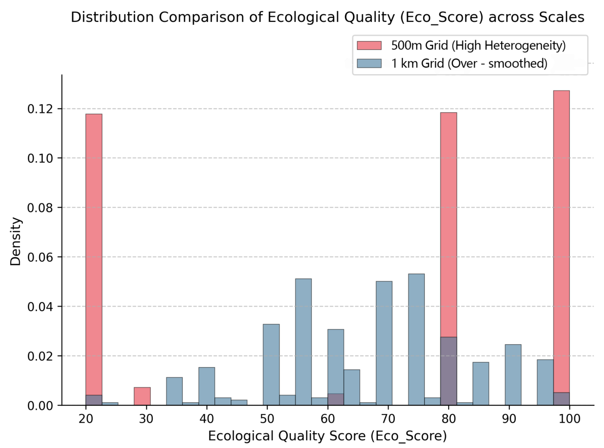
② Gridding processing and scale justification. A 500 m × 500 m equidistant grid was used as the basic analysis unit. Raster data were resampled using bilinear interpolation to minimize spatial accuracy loss. Crucially, the 500 m × 500 m analytical grid balances spatial heterogeneity with the need for scale-appropriate sustainability analysis and reduces aggregation bias associated with the Modifiable Areal Unit Problem (MAUP). Comparative statistical diagnostics between the 500 m and 1 km aggregated grids (see Figure 6) reveal severe over-smoothing at the coarser resolution. Specifically, upscaling to 1 km artificially neutralizes the extreme ecological scores (e.g., highly artificialized built-up zones and pristine core habitats), artificially compressing the variance towards the median. The 500 m grid retains these localized extreme values, thereby preventing statistical masking and ensuring that the subsequent XGBoost–SHAP framework can capture non-linear empirical patterns and spatial thresholds associated with localized anthropogenic stress.
(3) Data cube construction, data cleaning, and quality control. Using the “Attribute Join” and “Zonal Statistics” functions in QGIS 3.44.5, this study merged the 1468 tourism resource points with their corresponding environmental predictor values extracted from the 500 m × 500 m grid cells. The construction of the final modelling dataset followed a standardized preprocessing workflow. First, all vector and raster datasets were reprojected to WGS 84/UTM zone 52N (EPSG:32652) to ensure geometric consistency. Second, raster layers were clipped to the same analytical boundary and resampled to the 500 m grid resolution. Third, duplicate tourism-resource records, invalid geometries, and points falling outside the study boundary were checked and removed where necessary. Fourth, each tourism resource point was spatially joined to the corresponding grid cell to obtain the ecological quality score and explanatory variables.
Missing values were handled according to their source and spatial meaning. If a missing value resulted from a tourism resource point falling outside the valid raster coverage, the point was excluded from the modelling dataset because interpolation would introduce artificial ecological information. For continuous raster-derived variables with isolated missing grid values inside the valid study area, the value was filled using the mean of neighboring valid grid cells within a 3 × 3 moving window. Variables with zero values that reflected real spatial conditions, such as very low population density or GDP intensity, were retained rather than treated as missing values. After preprocessing, the final feature matrix contained 1468 valid observation records, each covering the dependent variable Eco_Score and seven explanatory variables representing topography, socioeconomic pressure, and spatial accessibility.
Outliers were identified using both statistical and spatial diagnostics. For each continuous predictor, boxplots, z-scores, and the interquartile range method were used to detect extreme values. Observations exceeding three standard deviations from the mean or falling outside 1.5 times the interquartile range were further examined in GIS to determine whether they represented data errors or genuine spatial extremes. Because the study area contains highly heterogeneous landscapes, extreme values such as high population density in urban nodes, very high elevation in mountainous areas, or very short distances to roads and water systems were retained if they corresponded to real geographic conditions. Erroneous values caused by spatial overlay errors, invalid raster cells, or duplicate records were corrected or removed. This procedure ensured that the model preserved meaningful spatial heterogeneity while minimizing the influence of data-processing artifacts.
Technological tools and computational environment. To improve reproducibility, all geospatial preprocessing and spatial feature extraction procedures were implemented using QGIS 3.44.5. Coordinate transformation, raster clipping, raster resampling, kernel density estimation, Euclidean distance calculation, attribute joining, and zonal statistics were conducted using the native QGIS geoprocessing toolbox. Subsequent statistical modelling, machine learning, explainable artificial intelligence analysis, and multi-objective optimization were implemented in Python 3.12. Data cleaning and matrix construction were performed using pandas and NumPy; PCA, multiple linear regression, random forest modelling, model evaluation, and cross-validation were implemented using scikit-learn; XGBoost modelling was implemented using the XGBoost package; Bayesian hyperparameter optimization was conducted using the Bayesian-optimization package; SHAP attribution and interaction analyses were performed using the shap package; and NSGA-II multi-objective optimization was implemented using the pymoo evolutionary optimization library.
For computational reproducibility, all continuous variables were stored in a unified tabular matrix after spatial extraction, and the same random seed was used for data partitioning, Bayesian optimization, and model training. Model inputs, preprocessing parameters, hyperparameter search ranges, and final optimized parameters were recorded to ensure that the analytical workflow could be repeated. Spatial visualization and cartographic outputs were produced using QGIS and Python visualization libraries. The processed dataset and code can be made available upon reasonable request, subject to data-source licensing restrictions.

2.3. A Data-Driven Analytical Framework

2.3.1. PCA-Based Feature Engineering

In complex social–ecological systems, predictor variables naturally exhibit strong spatial covariance. For instance, population aggregations consistently align with high economic output zones, while localized terrain features inherently covary with macro-elevation gradients. Feeding these raw, correlated indicators directly into the model can inflate local variance and obscure the empirical spatial patterns extracted by the downstream explainable artificial intelligence module. To resolve this problem, Principal Component Analysis (PCA) was implemented as a mathematical precursor to decouple the socioeconomic and topographic indicators, thereby constructing an orthogonal feature space.
Before PCA, all continuous predictors were standardized using z-score normalization, so that variables measured in different units, such as elevation, slope, population density, GDP intensity, and distance measures, contributed to the PCA on a comparable scale. This step is essential because PCA is sensitive to variable scaling; without standardization, variables with larger numerical ranges could dominate the extracted components. To assess the sensitivity of PCA results to scaling, the component structure obtained from standardized variables was compared with alternative preprocessing settings, including Min–Max normalization and the raw unstandardized input matrix. The standardized solution was retained because it produced a more balanced loading structure and clearer geographical interpretation of the principal components.
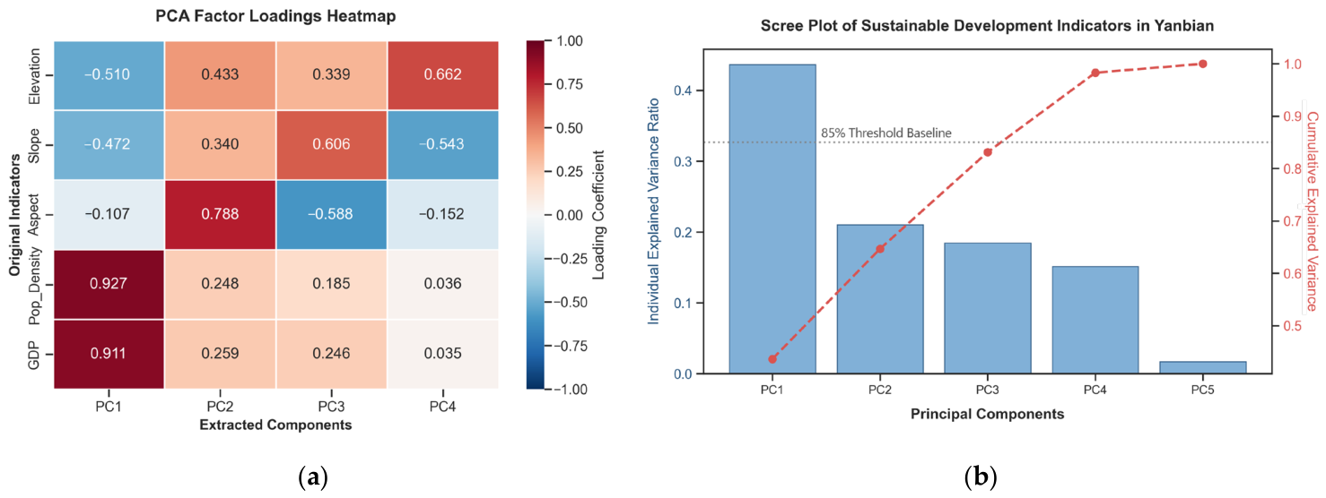
The efficiency of this dimensional reduction was evaluated through the individual and cumulative explained variance ratios (Figure 7b). The scree plot indicates a steep initial decline, with the first three principal components collectively capturing the vast majority of the original dataset’s spatial variance. Retaining these components effectively preserves the core environmental variability while stripping away redundant background noise.
The physical and geographical semantics of the extracted orthogonal components were decoded through the factor-loading heatmap (Figure 7a). PC1 captures the primary variance of the dataset and is characterized by high positive loadings for GDP (0.927) and population density (0.788). Therefore, PC1 is interpreted as a comprehensive proxy for “Socioeconomic Pressure.” PC2 exhibits a strong loading on elevation (0.911), representing the regional “Macro-topographic Base.” PC3 captures “Micro-topographic Complexity,” with high loadings on aspect (0.662) and slope (0.506).
Because SHAP is applied to PCA-derived components rather than directly to the original variables, the resulting SHAP values should be interpreted at the component level. This transformation has two implications. First, SHAP values represent the marginal contribution of orthogonal latent dimensions, such as socioeconomic pressure or macro-topographic background, rather than the independent effect of a single raw variable. Second, any interpretation of original drivers, such as GDP, population density, elevation, or slope, must be made through a secondary back-mapping step based on PCA loadings. This approach reduces multicollinearity and produces more stable model attribution, but it also reduces the directness of variable-level interpretation. Therefore, in this study, SHAP results are reported primarily at the component level, and references to original variables are made only when the corresponding PCA loadings provide a clear physical or socioeconomic meaning. This clarification prevents overinterpreting PCA-based SHAP values as direct causal effects of individual raw variables.

2.3.2. XGBoost Modeling and Spatial Validation

The Extreme Gradient Boosting (XGBoost) algorithm was employed to capture the complex, non-linear empirical associations between the orthogonal predictors and ecological quality. The model was implemented in Python using the xgboost package, while data partitioning, benchmark model construction, performance evaluation, and cross-validation procedures were conducted using scikit-learn. To mitigate structural overfitting and maximize predictive efficacy, a Bayesian optimization framework was implemented to systematically search the hyperparameter space. The optimized hyperparameters included n_estimators, learning_rate, max_depth, subsample, colsample_bytree, reg_alpha, and reg_lambda. The search ranges were defined to cover both conservative and flexible model configurations, allowing the algorithm to balance model complexity, regularization strength, and generalization capacity.
The objective function of Bayesian optimization was to maximize cross-validated R2 while simultaneously monitoring RMSE and MAE. The optimization process was run for 100 iterations, and convergence was evaluated by examining whether the best validation score stabilized during the final iterations. The optimal configuration was selected only when additional iterations produced negligible improvement in the validation objective, indicating that the search had approached a stable region of the hyperparameter space. To ensure reproducibility, the random seed was fixed during data partitioning, cross-validation, and model fitting. The final optimized hyperparameters are summarized in Table 3.
The selected hyperparameters reflect a strategy focused on robust ensemble learning. A relatively low learning rate (0.0332) coupled with a substantial number of estimators (1390) allows the model to incrementally refine its predictive capacity, thereby minimizing the risk of rapid overfitting. To prevent the model from capturing localized noise, the tree depth was capped at 6, while the inclusion of L2 regularization (reg_lambda = 5.5010) and L1 regularization (reg_alpha = 0.001741) ensures that the weight distribution remains constrained. Furthermore, the subsample and colsample_bytree ratios (0.618992 and 0.816483, respectively) introduce necessary stochasticity, reducing correlation between individual trees and enhancing the overall stability of the ensemble. This optimized configuration yielded a peak cross-validated R2 of 0.9389, an RMSE of 9.012, and an MAE of 6.205, indicating strong apparent predictive performance under conventional cross-validation prior to spatial validation. In addition to the optimized parameter values, model stability was evaluated by comparing the performance of the Bayesian-optimized XGBoost model with benchmark models and by examining the consistency between conventional random cross-validation and spatial block cross-validation. This comparison was necessary because high performance under random partitioning may partly reflect spatial autocorrelation rather than true geographic transferability. Therefore, the optimized model was not accepted solely on the basis of the highest cross-validated R2; it was further evaluated using spatially independent validation blocks to assess whether the learned relationships could generalize to geographically distinct areas.
Geospatial data inherently exhibit strong spatial autocorrelation, presenting unique methodological challenges for evaluating the generalization robustness of machine learning models. Standard random cross-validation partitions samples stochastically, frequently assigning geographically adjacent grid cells into both training and testing subsets. This proximity induces severe spatial data leakage, enabling the algorithm to achieve artificially inflated accuracy metrics by merely memorizing local clustering traits. Consequently, traditional validation configurations fail to reflect the model’s true extrapolation capacity in unsampled geographic regions.
To rigorously evaluate spatial robustness, a Spatial Block Cross-Validation (Spatial Block CV) architecture was integrated. This approach partitions the study area into discrete, non-overlapping geometric blocks based strictly on spatial coordinates. During each validation iteration, the model is trained on a subset of spatial blocks and tested on geographically independent blocks that were not used during training. This design reduces spatial data leakage caused by neighboring samples being assigned simultaneously to training and testing subsets.
For transparency, the spatial validation results were reported using fold-level performance statistics rather than a single accuracy value. The median R2, RMSE, and MAE across spatial blocks were used as the primary indicators of spatial transferability, while the dispersion across folds was interpreted as an uncertainty signal for geographically unsampled areas. In addition to Random Cross-Validation and Spatial Block Cross-Validation, the model was benchmarked against Multiple Linear Regression and Random Forest to examine whether the observed performance gain was specific to XGBoost or reflected a more general non-linear modelling advantage. Because fully independent external validation data were not available for this corridor, alternative spatial validation designs, such as different block sizes, leave-one-region-out validation, or external testing in another tourism corridor, are identified as important robustness extensions for future research.

2.3.3. SHAP Explainable Module

To interpret the highly non-linear associations captured by the tree-based ensemble model, this study utilized the Shapley Additive exPlanations (SHAP) framework grounded in cooperative game theory. The SHAP analysis was implemented in Python using the shap package, including global feature-importance ranking, local dependence analysis, and second-order interaction attribution. Unlike traditional heuristic feature importance metrics, which frequently suffer from inconsistency and scale mismatches, SHAP provides mathematically validated feature attributions by calculating the marginal contribution of each variable across all possible feature combinations. The framework operates as an additive feature attribution method, decomposing the local prediction f(x) for any individual spatial observation x into a linear summation of the baseline expected value and the localized feature attributions:
  g ( z ) =   ϕ 0 + i = 1 M ϕ i z i
where g(z′) represents the explanatory model, Φ0 is the baseline expected value across the entire training dataset, M is the total number of predictors, and Φi∈R denotes the SHAP value allocated to the i-th predictor variable. This mathematical configuration satisfies the essential axioms of local accuracy, missingness, and consistency, ensuring that the computed attributions possess the same units and scale as the target ecological quality profile.
The extraction of empirical statistical patterns spans multiple analytical scales within this framework. Globally, the comprehensive contribution of each orthogonal principal component and spatial accessibility metric is quantified by aggregating the absolute SHAP values across all N observation records:
I i   =   1 N j = 1 N | ϕ i ( j ) |
This aggregate importance metric provides an objective, global ranking of the structural variables influencing regional ecological variance. To capture localized non-linear dependence characteristics and identify critical thresholds, individual predictor values are plotted against their corresponding localized SHAP values. This approach uncovers the precise continuous trajectories and mathematical turning points where ecological configurations demonstrate abrupt responses to demographic or infrastructural modifications.
To deconstruct the complex multi-dimensional interdependencies inherent within the social–ecological landscape, the framework isolates second-order interaction patterns. The SHAP interaction value (Φi,j) splits the joint attribution between variable pairs into distinct main and joint effects based on the Owen value for cooperative games:
Φ i , j   = S \ { i , j } | S | ! ( M | S | 2 ) ! 2 ( M 1 ) ! [ f ( S { i , j } ) f ( S { i } ) f ( S { j } ) + f ( S ) ]
When i ≠ j, Φi,j isolates the pure synergistic or antagonistic statistical attribution between the two predictors, effectively factoring out the standalone linear and non-linear effects of each individual variable. This quantitative isolation maps out how natural geomorphic features attenuate or intensify the statistical externalities of socioeconomic pressures, thereby translating opaque machine learning black-box predictions into transparent, actionable spatial intelligence for regional sustainable planning.

2.3.4. NSGA-II Multi-Objective Optimization

To navigate the inherent trade-offs between ecological conservation and socioeconomic development, a Multi-Objective Optimization (MOO) framework was formulated based on the Non-dominated Sorting Genetic Algorithm II (NSGA-II). The optimization procedure was implemented in Python using an evolutionary multi-objective optimization library, which allowed the definition of objective functions, constraints, population size, crossover probability, non-dominated sorting, crowding-distance calculation, and hypervolume-based convergence monitoring. The selection of NSGA-II was based on a comparison with several commonly used multi-criteria optimization and decision-making approaches. Weighted-sum optimization can transform multiple objectives into a single objective, but it requires subjective weight assignment and may fail to identify non-convex parts of the trade-off surface. AHP is useful for structuring expert preferences, but it is less suitable for automatically searching large spatial configuration spaces. TOPSIS can rank predefined alternatives according to their distance from ideal and negative-ideal solutions, but it does not generate new spatial configurations or a continuous Pareto frontier. MOPSO and other swarm-based algorithms can also solve multi-objective problems, but NSGA-II has been widely used in spatial optimization because its non-dominated sorting and crowding-distance mechanisms maintain both convergence toward the Pareto frontier and diversity among alternative solutions. Therefore, NSGA-II was selected because the objective of this study is not to select a single best scenario based on predefined weights, but to reveal the full trade-off structure between ecological integrity and socioeconomic development potential (Table 4).
This framework seeks to identify a set of Pareto-optimal spatial configurations that simultaneously maximize the aggregated ecological quality score and the latent socioeconomic potential across the study area.
The optimization objectives were defined as follows:
(1)
Maximize Ecological Integrity: Attaining the highest regional average Eco_Score by prioritizing the spatial clustering of high-value ecological patches.
(2)
Maximize Socioeconomic Potential: Enhancing the accessibility of tourism resources to stimulate regional economic vitality, represented by the synthesized potential index derived from the XGBoost predictive model.
The optimization process operates within a constrained feasible space defined by physical and administrative boundaries. We imposed a “non-deterioration constraint,” mandating that the mean ecological quality of any optimized spatial unit must not fall below the baseline established by the current land-use configuration. To ensure the physical realism of the optimized solutions, spatial contiguity constraints were integrated, preventing the generation of fragmented or biologically inviable land-use patches.
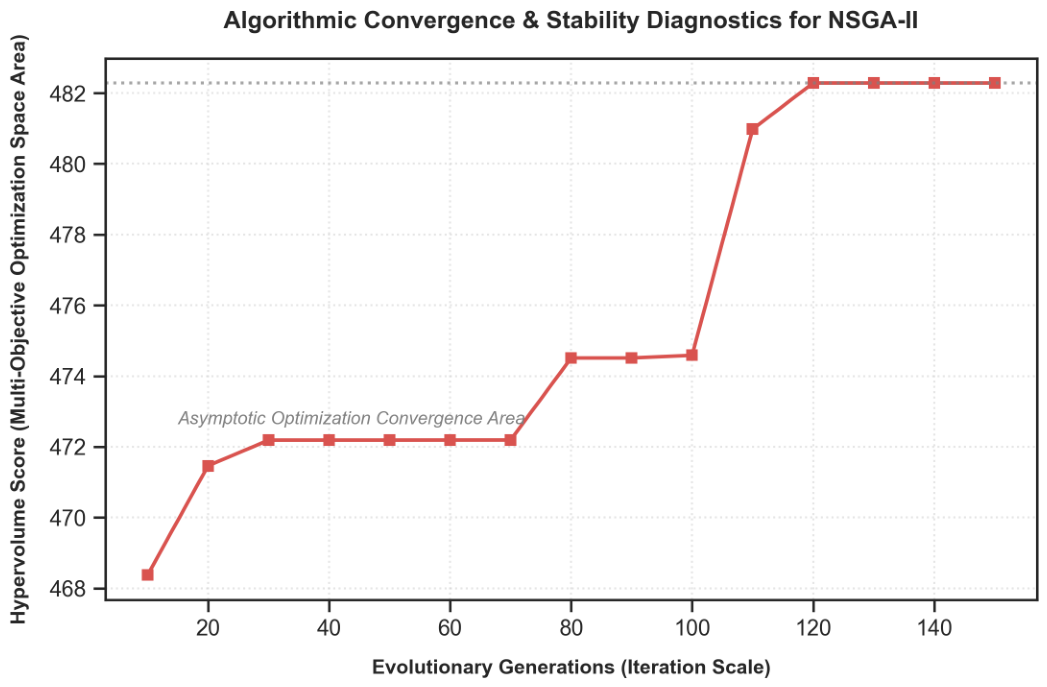
The algorithm utilizes a binary-coded genetic structure, with a population size of 200 and a crossover probability of 0.9. The fitness of each spatial configuration is evaluated through an elite-preservation mechanism, which ranks candidate solutions based on non-dominated sorting and crowding distance. This mechanism is central to the choice of NSGA-II because it allows the model to retain multiple feasible planning alternatives rather than forcing the decision into a single weighted optimum. In this way, NSGA-II provides a more informative decision-support structure than single-score multi-criteria methods, especially when ecological protection and socioeconomic development cannot be reduced to one fixed preference weight. The algorithmic stability was monitored using the hypervolume indicator across 150 evolutionary generations. The convergence diagnosis shows that the hypervolume curve plateaued after approximately 120 generations, indicating that the derived Pareto front had approached a stable solution set. The resulting set of optimal solutions provides a systematic quantitative basis for decision-makers to evaluate the trade-offs between conflicting spatial development goals.

3. Results

3.1. Model Performance and Spatial Robustness

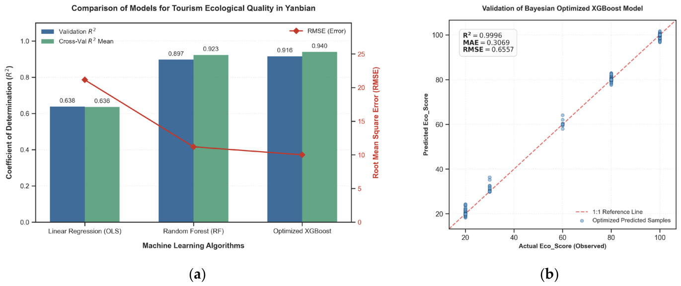
To evaluate the predictive efficacy of the Bayesian-optimized XGBoost model, its performance was benchmarked against traditional Multiple Linear Regression (MLR) and the Random Forest (RF) algorithm. As illustrated in the model comparison analysis (Figure 8a), the MLR model exhibited limited fitting capacity, yielding a cross-validation R2 of 0.636 and an RMSE exceeding 18. This performance discrepancy suggests that the environmental predictors share highly non-linear associations with ecological quality rather than following a simple linear superposition.
In contrast, ensemble tree-based algorithms significantly enhanced predictive accuracy. The optimized XGBoost model emerged as the most robust framework, achieving the highest cross-validation coefficient of determination (R2 = 0.9389) and the lowest prediction errors (RMSE = 9.012, MAE = 6.205), thereby outperforming the RF model. Furthermore, the validation scatter plot indicates strong agreement between predicted and observed Eco_Score on the designated validation set, with data points tightly clustered along the 1:1 reference line (Figure 8b). The associated statistics were R2 = 0.9996, RMSE = 0.6557, and MAE = 0.3069. However, this high apparent fit should be interpreted together with the Spatial Block Cross-Validation results to avoid overstating geographic generalization. Taken together, these results suggest that the model captured complex associations among topographic, socioeconomic, and spatial accessibility variables, while its transferability should still be interpreted cautiously.
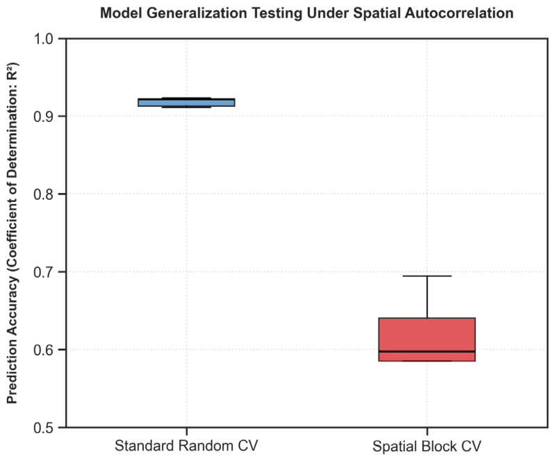
Beyond standard performance metrics, we further assessed the spatial generalization capacity of the model to address the potential influence of spatial autocorrelation. The comparison between Standard Random Cross-Validation (Random CV) and Spatial Block Cross-Validation (Spatial Block CV) is presented in Figure 9. Random CV produced an R2 exceeding 0.90, whereas Spatial Block CV yielded a more conservative median R2 of approximately 0.60. This substantial reduction indicates that part of the apparent predictive performance under random partitioning was influenced by spatial dependence among neighboring samples. In other words, when geographically adjacent observations are randomly split between training and testing sets, the model may partly benefit from local spatial similarity rather than fully transferable ecological relationships.
The Spatial Block CV result should therefore be interpreted not as a model failure, but as a more realistic estimate of prediction performance in geographically independent areas. A median R2 of approximately 0.60 indicates moderate spatial transferability under a stringent validation design. This level of performance is adequate for strategic planning applications that require relative prioritization, identification of broad vulnerability gradients, and comparison of governance scenarios. However, it is not sufficient to support precise parcel-level prediction or deterministic site-specific decision-making in unsampled areas. For this reason, the subsequent SHAP interpretation and NSGA-II optimization are used primarily to support spatial diagnosis and scenario comparison rather than to produce exact ecological forecasts for every grid cell.
The discrepancy between Random CV and Spatial Block CV also highlights the uncertainty associated with predictions in unsampled or weakly represented geographic contexts. Areas that differ strongly from the training blocks in terms of topography, accessibility, land-use composition, or socioeconomic pressure may have higher prediction uncertainty. Therefore, model outputs should be interpreted together with field knowledge, ecological monitoring, and planning constraints. In practical terms, the model provides a decision-support tool for identifying where ecological pressure is likely to concentrate and where governance intervention should be prioritized, but it should not replace site-level ecological assessment.
Although Bayesian optimization improves hyperparameter selection and reduces arbitrary model tuning, it does not completely eliminate the risk of overfitting. This risk is especially relevant in spatial datasets because high predictive accuracy may reflect local clustering patterns rather than generalizable mechanisms. To reduce this risk, the optimized XGBoost model was constrained through a relatively low learning rate, limited tree depth, L1 and L2 regularization, subsampling, and column sampling. In addition, the model was evaluated against benchmark models and assessed using Spatial Block CV. These procedures provide a more conservative evaluation of model performance and reduce the likelihood that the subsequent interpretation is based only on local spatial memorization. Nevertheless, the remaining performance gap between Random CV and Spatial Block CV suggests that model outputs should be interpreted with uncertainty, especially when extrapolated to areas outside the spatial structure represented in the training data.

3.2. Global Contributions to Ecological Quality

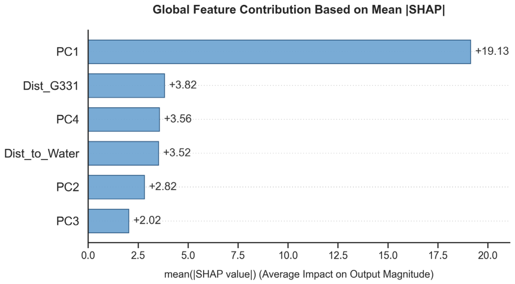
The global influence of environmental predictors on ecological quality is quantified through the aggregation of absolute SHAP values, as illustrated in the feature importance ranking (Figure 10). This diagnostic analysis reveals a hierarchical structure of determinants, wherein socioeconomic pressure represented by PC1 exerts a dominant influence, with a mean SHAP value of 19.13. This magnitude significantly surpasses the contributions of secondary spatial factors, including the distance to the G331 national highway (3.82), PC4 (3.56), distance to water (3.52), PC2 (2.82), and PC3 (2.02). The overwhelming importance of PC1 underscores that within the study area, the intensity of human-induced socioeconomic activity remains the primary driver of ecological variance, dwarfing the relative impact of natural geomorphic substrates.
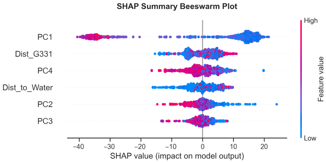
To further deconstruct the directionality and distribution of these impacts, the SHAP summary beeswarm plot (Figure 11) provides a detailed mapping of how feature values correlate with model outputs. The distribution of PC1 is particularly revealing, exhibiting a pronounced bifurcation. High PC1 values (depicted in red) are predominantly associated with substantial negative SHAP values, indicating that intense socioeconomic pressure acts as a consistent force for ecological degradation. Conversely, low PC1 values (depicted in blue) cluster toward positive SHAP values, representing the ecological “buffer zones” where human interference is minimal.
The remaining predictors exhibit more nuanced, symmetric response patterns. For Dist_G331 and Dist_to_Water, the distribution demonstrates that proximity (low feature values, shown in blue) generally correlates with higher ecological scores, suggesting that the development corridor and riparian zones contain the most concentrated anthropogenic pressure. PC2 and PC3, which encapsulate topographical attributes, display broader clusters centered near zero, implying that while these variables contribute to localized ecological variability, their global effect is less deterministic than that of the primary socioeconomic dimensions. The dispersion of these points indicates that the influence of topography on ecological quality is highly conditional and sensitive to the specific context of each spatial unit, rather than operating through a singular, uniform gradient. Collectively, these patterns confirm that while topographical factors provide the physical substrate, the overarching ecological configuration of the tourism corridor is fundamentally reshaped by the non-linear interaction between anthropogenic encroachment and spatial accessibility.

3.3. Non-Linear Responses and Interaction Patterns

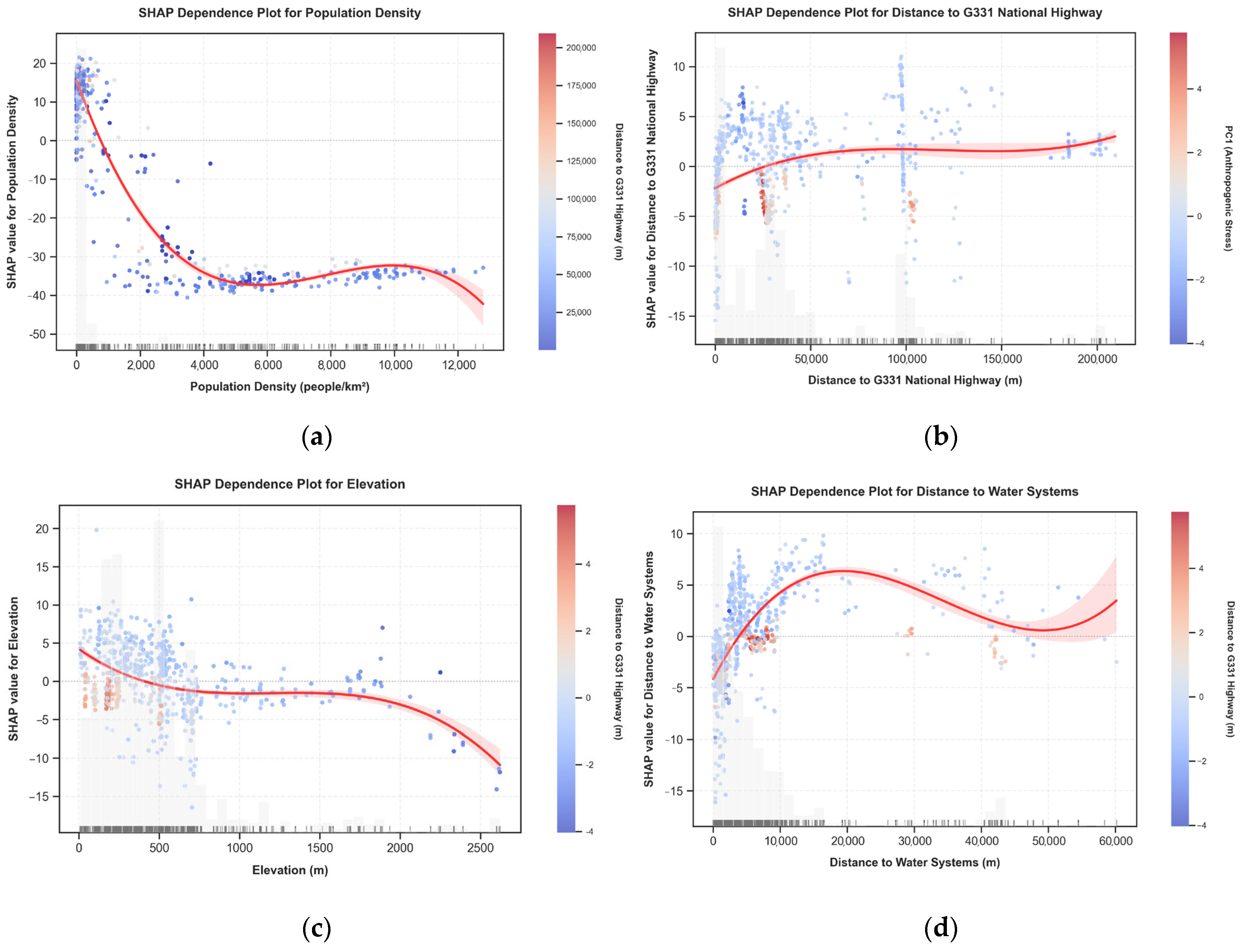
The SHAP dependence plots provide a granular perspective on the non-linear response mechanisms between environmental predictors and ecological quality, revealing distinct spatial thresholds that govern the social–ecological equilibrium of the corridor (Figure 12).
The response pattern for population density (Figure 12a) is characterized by a steep, concave-downward trajectory. Ecological quality declines rapidly as population density increases from low-density conditions to approximately 4000 people/km2, identifying this interval as the primary “degradation threshold” of the corridor. This pattern can be explained by the early-stage conversion mechanism emphasized in tourism planning and landscape ecology: when population and service activities begin to concentrate around tourism nodes, the first wave of land conversion, road-side construction, parking facilities, accommodation expansion, and supporting infrastructure often replaces or fragments relatively intact landscape patches. Therefore, ecological degradation accelerates before the threshold because low- to medium-density expansion tends to occur at the expense of previously undeveloped or semi-natural land.
Beyond approximately 4000 people/km2, the marginal ecological cost diminishes. This does not mean that high-density development is ecologically harmless; rather, it suggests that many high-density areas have already experienced substantial anthropogenic conversion, leaving fewer remaining natural patches to be further degraded. In tourism-planning terms, the threshold reflects a shift from extensive land conversion to intensified use within already transformed spaces. The color-coded interaction with the distance to the G331 highway further indicates that high-density clusters located close to the road corridor experience more severe ecological deficits than isolated clusters, confirming that demographic concentration and infrastructural accessibility jointly produce cumulative pressure. This mechanism is consistent with protected-area and transportation-corridor studies showing that ecological impacts often intensify where visitor concentration, accessibility improvement, and land development overlap.
Regarding the spatial accessibility factors, the dependence plots for distance to the G331 National Highway (Figure 12b) and distance to water systems (Figure 12d) exhibit non-monotonic, hump-shaped trajectories. For the G331 highway, ecological quality improves as distance from the road increases and reaches relative stabilization at approximately 50,000 to 100,000 m. This pattern should be interpreted as a corridor influence zone rather than a universal fixed-distance buffer. In tourism corridors, roads do not only provide mobility; they reorganize land markets, visitor flows, service facilities, parking demand, informal commercial development, and access to scenic resources. As a result, road proximity may generate ecological disturbance through habitat fragmentation, edge effects, waste discharge, noise, construction spillover, and induced tourism development.
The water-distance response shows a similar planning mechanism. Ecological quality increases up to approximately 20,000 m from water systems, suggesting a transition from highly attractive riparian tourism spaces to less disturbed interior forest patches. Water bodies are often core scenic resources, but they also attract accommodation, leisure facilities, waterfront trails, and visitor concentration. Therefore, riparian zones may experience simultaneous ecological value and development pressure. The combined G331 and water-distance thresholds indicate that ecological vulnerability is highest where road-based accessibility and water-based tourism attractiveness overlap. This finding is consistent with carrying-capacity and protected-area management studies showing that ecological degradation is frequently concentrated in accessible scenic nodes, trail corridors, waterfront areas, and transport-connected tourism belts.
Elevation (Figure 12c) acts as a structural stabilizer within the corridor, displaying a generally negative correlation with ecological degradation as altitude increases. While lower altitudes are associated with highly variable SHAP values, reflecting the intense competition between urban development and riparian habitats, higher altitudes (exceeding 1500 m) exhibit a more consistent negative impact on ecological scores. This decline at high elevations indicates the restricted capacity of alpine environments to maintain complex ecological structures under the pressures of the tourism corridor. These trajectories confirm that ecological vulnerability is intrinsically linked to demographic and infrastructural thresholds, such as the 4000 people/km2 density peak and the 50 km corridor-influence zone, which should serve as the primary criteria for adaptive spatial governance. These thresholds suggest that effective conservation management must be highly localized, as the ecological sensitivity of the landscape is fundamentally contingent upon the proximity to both human infrastructure and water-based tourism attractions.

3.4. Synergistic and Antagonistic Interaction Patterns

To deconstruct the multi-dimensional dependencies within the study area, we examined second-order SHAP interaction values, which isolate the joint effects of predictor pairs from their independent contributions. The interaction patterns, illustrated in Figure 13, reveal how socioeconomic and geomorphic constraints modulate ecological quality across different spatial contexts.
The interaction between population density and GDP (Figure 13a) exhibits a distinct saturation and reversal effect. At lower population densities, GDP may coexist with relatively higher ecological quality because economic activity in these areas is often associated with dispersed services, limited land conversion, or tourism functions embedded within a still-dominant natural landscape. However, once population density exceeds approximately 4000 people/km2, the interaction becomes antagonistic. This reversal suggests that economic output and population concentration begin to reinforce each other through construction demand, road-side development, service expansion, and intensified land-use conversion. In other words, the ecological meaning of GDP depends on the density context: in low-density areas it may reflect limited or compatible activity, whereas in high-density tourism nodes it becomes coupled with physical expansion and cumulative disturbance. This explains why ecological degradation accelerates before the threshold and why further increases after the threshold produce smaller marginal losses: the major ecological conversion has already occurred during the transition from low-density landscape to dense development node.
The corridor-valley effect (Figure 13b), represented by the interaction between the distance to the G331 highway and distance to water, highlights the spatial concentration of anthropogenic stress. We observe that near the highway (low distance values), the interaction value fluctuates significantly, indicating that the proximity to riparian zones creates a high-pressure environment where road-based tourism development and water-source exploitation intersect. This interaction is most intense within a 20 km radius of the highway, identifying this zone as the critical spatial intersection where human-induced habitat fragmentation is most pronounced.
Finally, the phenomenon of topographic shielding (Figure 13c), captured by the interaction between elevation and PC1 (socioeconomic pressure), demonstrates that high-altitude environments act as a structural constraint on the influence of socioeconomic stressors. In lowland areas, PC1 shows a strong negative interaction with elevation, reflecting the ease of human encroachment into accessible valleys. Conversely, as elevation increases, the SHAP interaction value trends downward, confirming that mountainous terrain provides a natural “shielding” effect that dampens the ecological impact of socioeconomic pressures. This finding proves that high-elevation units retain a degree of ecological resilience even when subjected to high socioeconomic stress, positioning these areas as essential refugia for biodiversity within the tourism corridor. Collectively, these interaction patterns delineate a tripartite spatial structure: high-pressure urbanized clusters, vulnerable riparian-corridor interfaces, and resilient high-altitude ecological refugia, each requiring distinct management interventions.

3.5. Local Interpretability of Typical Sites

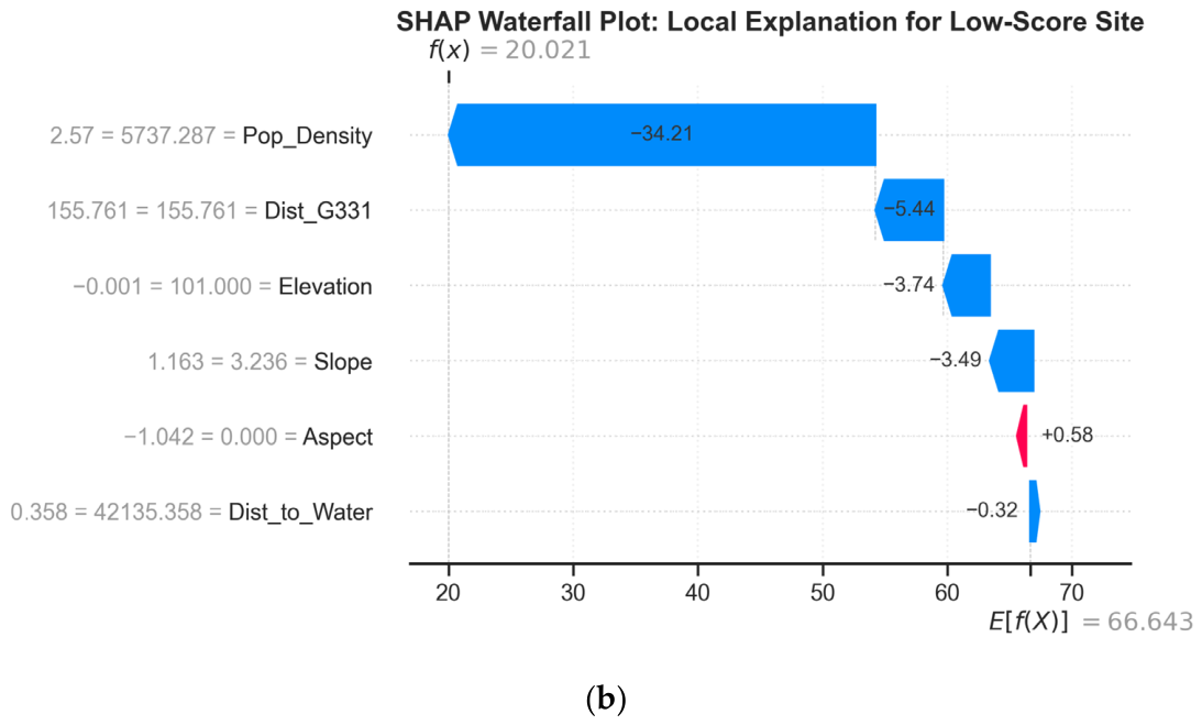
To translate abstract model outputs into concrete, site-specific spatial intelligence, we employed SHAP waterfall plots to deconstruct the local prediction logic for two archetypal locations: a high-performing site situated within a protected ecological core and a low-performing site constrained by intensive anthropogenic development (Figure 14).
The high-scoring site (Figure 14a) demonstrates a robust ecological baseline, where the prediction is driven by favorable structural variables. In this instance, the positive influence of high-altitude topographical positioning and the substantial distance from the G331 highway serve as the primary drivers, pushing the final score significantly above the base value (E[f(x)]). The minimal contribution of population density confirms that the site remains sequestered from the immediate pressures of the tourism corridor, allowing the intrinsic ecological service capacity to dominate the final prediction.
Conversely, the low-scoring site (Figure 14b) illustrates a regime dominated by socioeconomic stressors. Here, the proximity to the G331 highway and a dense population footprint act as aggressive antagonistic forces, pulling the score downward from the expected baseline. The negative marginal contribution of these variables highlights the site’s vulnerability to infrastructural encroachment. Interestingly, even where some natural topographic features provide minor positive support, they are insufficient to offset the compounding ecological deficit induced by high human accessibility.
These waterfall plots demonstrate that the model’s predictive power is not merely a product of global correlations, but rather a reflection of site-specific competitive dynamics. By isolating the precise marginal contribution of each variable, we identify that the “ecological failure” of low-scoring sites is seldom the result of a single factor, but rather the cumulative effect of spatial proximity to development axes and high demographic intensity. This local-level interpretability allows for a diagnostic approach to spatial planning, where managers can identify whether a site’s ecological degradation stems from excessive human influx, infrastructural fragmentation, or intrinsic topographical unsuitability, thereby enabling the implementation of precisely targeted conservation interventions.

4. Scenario Simulation and Spatial Optimization

4.1. Pareto Front Analysis

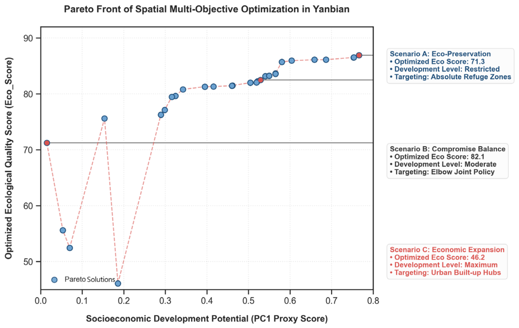
To resolve the inherent conflict between ecological conservation and socioeconomic expansion, this study utilized the NSGA-II algorithm to map the trade-off space between aggregated ecological quality and socioeconomic potential. The resulting Pareto front (Figure 15) illustrates a non-linear frontier where improvements in one objective inevitably necessitate a compromise in the other, providing a systematic quantitative basis for spatial policy formulation.
Compared with a weighted-sum or AHP-based approach, which would require assigning a fixed preference weight between ecological and socioeconomic objectives, the NSGA-II result preserves the full trade-off structure. This is important because the Pareto frontier shows that there is no single universally optimal solution; rather, different scenarios reflect different governance preferences. A purely ecological weighting would likely select a solution close to Scenario A, while a development-oriented weighting would likely select a solution close to Scenario C. However, these single-preference methods would make it difficult to identify the intermediate “elbow” region represented by Scenario B, where ecological quality can be substantially maintained while moderate socioeconomic vitality is still preserved. Therefore, the NSGA-II result provides more policy-relevant information than a single ranked outcome because it allows decision-makers to compare conservation-priority, compromise-balance, and development-priority pathways simultaneously.
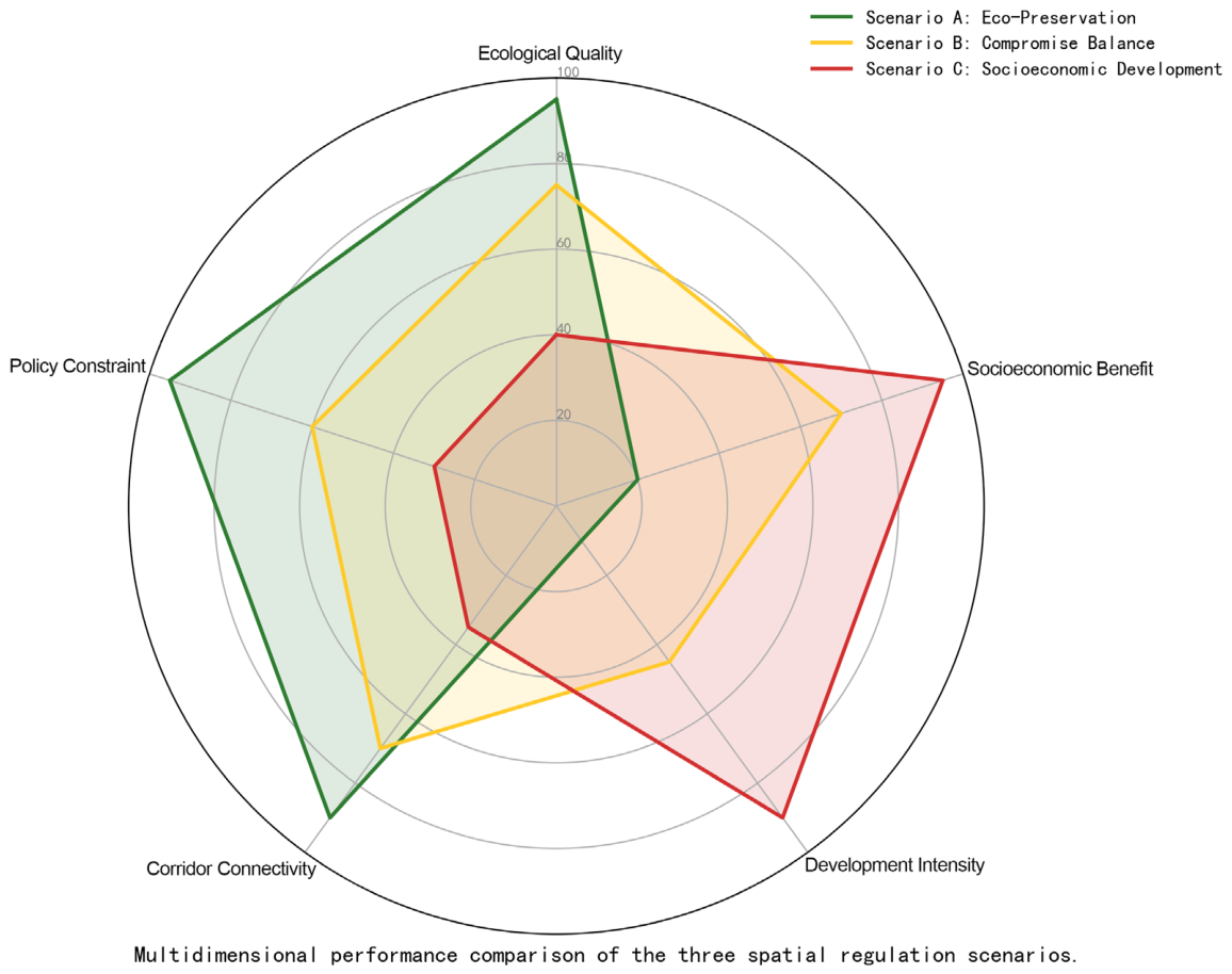
The optimization results reveal three distinct strategic clusters along the Pareto-optimal frontier, corresponding to varied land-use management priorities. Scenario A (Eco-Preservation) represents the upper-left segment of the frontier, characterized by high ecological quality (Eco_Score = 71.3) but minimal development potential. This scenario targets absolute ecological refuge zones, where land-use policy strictly prioritizes habitat connectivity and biodiversity preservation over infrastructure expansion. At the opposite extreme, Scenario C (Economic Expansion) occupies the lower-right segment, achieving high socioeconomic potential at the cost of significantly lower ecological scores (Eco_Score = 46.2). This configuration identifies urban built-up hubs where intense development is prioritized, yet warns of substantial ecological risks if left unmanaged.
The most critical finding resides in the “elbow” region of the Pareto front, represented by Scenario B (Compromise Balance). This configuration achieves a substantial optimization of ecological quality (Eco_Score = 82.1) while maintaining a moderate level of socioeconomic vitality. By adopting this “elbow joint” policy, decision-makers can effectively transcend the zero-sum nature of the trade-off, identifying spatial zones where well-planned tourism development can coexist with high-standard environmental stewardship. This multi-scenario analysis demonstrates that the corridor’s ecological stability is not a static property but a dynamic state dictated by the intensity and spatial arrangement of human activity. The Pareto-optimal set serves as a decision-support tool, enabling policymakers to evaluate the long-term ecological consequences of varied socioeconomic development targets before implementing region-wide land-use regulations.

4.2. Spatial Governance Scenarios

Based on the Pareto-optimal frontier identified in Section 4.1, we formulated three distinct spatial governance scenarios to provide a multidimensional decision-support framework for regional planning. As illustrated by the multidimensional performance radar chart (Figure 16), these scenarios translate abstract mathematical trade-offs into actionable land-use policies evaluated across five core axes: Ecological Quality, Socioeconomic Benefit, Development Intensity, Corridor Connectivity, and Policy Constraint.
(1) Scenario A: Eco-Preservation This scenario targets areas with the highest inherent ecological sensitivity, primarily encompassing core habitat patches and restricted biodiversity refugia. Spatial governance in this scenario is guided by a strict non-development directive. As reflected in the radar configuration, this scenario achieves peak values in Ecological Quality and Corridor Connectivity, driven by maximum Policy Constraint. By enforcing the maximum ecological quality threshold identified by the NSGA-II model, this configuration prohibits large-scale tourism infrastructure and mandates the restoration of fragmented habitat corridors. The primary objective is to maintain maximum connectivity within the ecological barrier, thereby positioning these zones as the foundation for the region’s long-term environmental sustainability.
(2) Scenario B: Compromise Balance Situated at the critical stabilization point of the Pareto frontier, this scenario optimizes the coexistence of tourism activities and ecological stewardship. The radar chart demonstrates a distinct geometric symmetry for this scenario, representing a strategic equilibrium across all five evaluative dimensions. The governance approach in this scenario shifts from total exclusion to compatible-use management. Land-use policies within these zones focus on the integration of low-impact tourism facilities (such as nature-based trails and low-density educational sites) that leverage existing accessibility without compromising core ecological integrity. This scenario identifies spatial patches where the marginal gain in Socioeconomic Benefit is maximized while maintaining Ecological Quality above the critical stability threshold, accompanied by moderate Development Intensity and balanced Policy Constraint.
(3) Scenario C: Socioeconomic Development This scenario focuses on urban hubs and existing intensive tourism zones where the primary objective shifts toward maximizing regional growth. The radar plot for this scenario exhibits a pronounced structural skew towards Socioeconomic Benefit and Development Intensity, offset by correspondingly low values in Policy Constraint and Corridor Connectivity. The governance approach is centered on intensive spatial planning, concentrating tourism-related socioeconomic activities within defined urban nodes to prevent sprawl-induced ecological degradation in the wider corridor. While this scenario accepts a lower baseline for average ecological quality, it mandates rigorous environmental engineering and waste management standards to ensure that the ecological footprint remains within regulated limits even under high-density development.

5. Discussion

5.1. Methodological Advantages

Beyond methodological performance, the proposed framework also advances the theoretical development of sustainability-oriented tourism corridor governance. The results support the view that tourism corridors should be understood as coupled social–ecological systems rather than as simple transportation belts or destination-development zones. In such systems, ecological vulnerability emerges from the interaction of socioeconomic pressure, accessibility concentration, land-use conditions, and topographic background. The observed non-linear and threshold-dependent patterns are consistent with sustainability science arguments that complex human–environment systems often involve tipping points, feedbacks, and spatial heterogeneity. The framework therefore translates abstract concepts such as coupling, vulnerability, resilience, and adaptive governance into measurable spatial relationships and actionable planning scenarios.
Compared with previous studies that assess tourism sustainability or social–ecological resilience mainly through composite indices, GIS-based suitability evaluation, or conventional regression models [3,4,6], the present framework provides three advantages. First, it does not treat ecological quality as a static suitability score, but models it as a non-linear response to interacting socioeconomic, accessibility, and topographic conditions. This is important for tourism corridors, where development pressure is concentrated along transport axes and tourism-resource clusters. Second, under conventional validation, the Bayesian-optimized XGBoost model achieved substantially higher predictive accuracy than the multiple linear regression model, suggesting that ecological responses along the corridor cannot be adequately captured by linear superposition alone. This interpretation is further qualified by the Spatial Block Cross-Validation results, which provide a more conservative assessment of geographic transferability. Third, the framework links prediction, explanation, and optimization within a single workflow. PCA reduces feature redundancy, XGBoost captures non-linear responses, SHAP reveals threshold-dependent mechanisms, Spatial Block Cross-Validation tests geographic transferability, and NSGA-II converts these diagnostic insights into spatial governance scenarios. Its value therefore lies not only in improving model performance, but also in converting the logic of corridor vulnerability into operational planning choices.
A further advantage of the proposed approach is that it explicitly addresses several weaknesses that remain common in spatial environmental modelling. Composite-index approaches are useful for rapid evaluation, but they often depend on predefined weights and may obscure threshold effects. Conventional regression models provide statistical transparency, but they are vulnerable to multicollinearity and may underrepresent non-linear ecological responses. Standard machine-learning models can improve prediction, but their results may be misleading when spatial autocorrelation is not properly controlled. In contrast, the present framework combines PCA-based feature orthogonalization, spatial block cross-validation, XGBoost prediction, SHAP interpretation, and NSGA-II optimization. The comparison between random cross-validation and spatial block cross-validation is especially important. Although random cross-validation produced an apparently high R2 above 0.90, the spatial block strategy generated a more conservative median R2 of approximately 0.60, revealing the risk of overestimating model performance under spatial data leakage [20,21]. This discrepancy has two implications. First, it confirms that ecological quality along the corridor is spatially structured, and that part of the predictive signal captured by random validation reflects local spatial dependence. Second, it suggests that planning applications should focus on robust spatial patterns, relative vulnerability gradients, and scenario-level trade-offs rather than exact prediction for individual unsampled locations.
From a governance perspective, this more conservative validation result is still useful. Corridor planning does not require the model to predict every grid cell with perfect accuracy; rather, it requires credible identification of pressure-sensitive zones, ecological buffers, and areas where development-conservation trade-offs are most pronounced. Therefore, the spatial block result supports the use of the model as a strategic decision-support tool, while also requiring caution in interpreting outputs for site-specific regulatory decisions. This interpretation strengthens the methodological credibility of the study because it explicitly distinguishes between predictive accuracy under spatial dependence and transferable planning knowledge under geographically independent validation.
These findings also clarify the tourism-specific meaning of ecological vulnerability in corridor landscapes. Tourism corridors differ from compact destinations because visitor flows, service facilities, scenic routes, and supporting infrastructure are organized along linear accessibility axes. As a result, ecological pressure is not generated only by the absolute number of tourists or facilities, but also by their spatial arrangement. The identified demographic threshold and road-influence buffer suggest that corridor tourism should be managed through spatial concentration rather than spatial diffusion. Concentrating tourism services in already developed or less sensitive nodes can reduce scattered land conversion, while strict ecological buffers are needed in riparian zones, road-adjacent belts, and habitat patches with high ecological value. At the same time, the topographic shielding effect indicates that high-altitude and steep-slope areas function as ecological refuges, because terrain constraints reduce direct human encroachment and help maintain biodiversity, water regulation, and landscape connectivity. This interpretation is consistent with landscape-ecology research emphasizing the protective role of terrain complexity, but the present study further quantifies how such topographic strengths interact with socioeconomic pressure in a tourism-corridor context.
The identified thresholds should be interpreted as context-specific empirical planning thresholds rather than universal standards. Similar studies of protected areas, scenic routes, and transportation corridors show that tourism-related ecological degradation often concentrates around accessible nodes, road corridors, waterfront attractions, and trail networks. However, the exact threshold values depend on landscape type, settlement density, infrastructure configuration, governance intensity, and ecosystem sensitivity. Thus, the contribution of this study is not the direct transferability of a 4000 people/km2 threshold or a 50 km road-influence zone, but the demonstration of a reproducible procedure for detecting threshold-dependent degradation and translating it into spatial governance.

5.2. Policy and Practical Implications for Sustainable Tourism

The empirical thresholds identified here suggest that uniform zoning is insufficient for corridor governance. Instead, spatial governance should combine ecological sensitivity, development intensity, corridor accessibility, and institutional responsibility. In planning practice, the three NSGA-II scenarios can be translated into strict conservation zones, compatible-use transition zones, and concentrated development zones. This zoning logic links optimization outputs with implementable corridor planning.
In practical planning terms, the population threshold can be interpreted as an early-warning boundary for development intensity rather than a strict administrative limit. Areas approaching the threshold should be monitored for rapid land conversion, roadside facility expansion, and increasing pressure on riparian or forest patches. Before the threshold is reached, planning intervention should focus on compact service consolidation, ecological design standards, wastewater and waste-management control, and prevention of scattered construction. After the threshold is exceeded, the planning priority should shift from expansion to redevelopment, restoration, and strict containment of additional land conversion. Similarly, the G331 influence zone suggests that road-adjacent areas should not be treated simply as development opportunity belts. They should be managed as multifunctional buffer spaces where tourism accessibility, ecological connectivity, habitat protection, and landscape restoration are coordinated.
This mechanism is particularly evident in the identified corridor-valley effect along the G331 national highway. The road-influence buffer and high-stress intersections near riparian zones indicate that these locations should be treated as ecological buffer belts and restoration priority zones. Rather than allowing dispersed tourism expansion, planning should encourage compact development in less sensitive locations, strengthen riparian protection, and restore fragmented habitats where road pressure is already high.
For Scenario A, namely the Eco-Preservation pathway, implementation should focus on strict ecological protection, habitat-connectivity maintenance, and restoration of fragmented ecological corridors. Large-scale tourism infrastructure, new accommodation clusters, and high-intensity commercial development should be restricted. Suitable interventions include ecological redline control, limited-access management, trail closure or rerouting in sensitive habitats, riparian-buffer restoration, forest-patch connectivity enhancement, and ecological monitoring stations. This scenario should be applied to core habitat patches, high-value forest and water-related ecosystems, steep-slope refuge areas, and zones where ecological quality is high but development pressure remains low.
For Scenario B, the Compromise Balance pathway, implementation should focus on compatible-use management. This scenario is the most practical option because it maintains ecological quality above the critical stability threshold while allowing moderate tourism development. Suitable interventions include low-impact nature trails, environmental education facilities, small-scale visitor-service points, eco-friendly viewing platforms, strict wastewater and solid-waste control, visitor-flow guidance, and ecological compensation for communities that restrict high-intensity development. Scenario B should therefore serve as the main governance model for transition zones where accessibility already exists but ecological degradation has not crossed the critical threshold.
For Scenario C, namely the Socioeconomic Development pathway, implementation should focus on concentrated development within existing urban hubs and intensive tourism-service nodes. The purpose is not to expand development everywhere, but to absorb tourism demand in already transformed areas and prevent scattered construction across the wider corridor. Suitable interventions include compact tourism-service clusters, redevelopment of existing built-up land, public-transport connection improvement, green infrastructure retrofitting, strict building-density control, environmental-impact assessment, wastewater-treatment upgrading, and waste-management standards. Scenario C should be accompanied by strong environmental regulation because it accepts lower ecological quality in exchange for higher socioeconomic benefits.
Institutional implementation requires a cross-jurisdictional corridor governance mechanism. Because the G331 corridor crosses multiple counties and connects ecological, transportation, tourism, and settlement systems, governance should not rely on a single department. A corridor-level coordination committee could be established to integrate the responsibilities of natural-resource authorities, ecological-environment departments, culture and tourism bureaus, transport agencies, county governments, and protected-area managers. Natural-resource authorities would be responsible for land-use zoning, ecological redline enforcement, and spatial planning control. Ecological-environment departments would monitor ecological quality, water quality, and pollution discharge. Culture and tourism bureaus would regulate tourism products, visitor-service facilities, and destination marketing. Transport agencies would manage road-side development, access control, and transport-related ecological mitigation. County governments would coordinate community participation, compensation mechanisms, and implementation financing. Such an institutional arrangement would help translate scenario-based optimization into enforceable spatial governance.
Adaptive management also requires a corridor-scale monitoring system. The monitoring system should include ecological indicators, tourism-pressure indicators, and governance-performance indicators. Ecological monitoring should track land-use change, forest and water-body integrity, habitat fragmentation, vegetation condition, riparian-buffer quality, and ecological restoration outcomes using remote sensing, field surveys, and ecological monitoring stations. Tourism-pressure monitoring should include visitor flows, accommodation capacity, parking demand, road traffic, waste generation, wastewater discharge, and seasonal crowding intensity. Governance-performance monitoring should evaluate whether development remains within designated zones, whether ecological buffers are maintained, whether restoration targets are achieved, and whether local communities receive compensation or livelihood benefits. These indicators should be updated periodically and linked to an adaptive feedback mechanism: if monitoring shows declining ecological quality or excessive tourism pressure, zoning intensity, visitor limits, infrastructure approval, and restoration priorities should be adjusted accordingly.
Potential stakeholder conflicts should also be explicitly considered. Scenario A may generate conflicts because strict conservation can limit tourism investment, local business opportunities, and community access to resources. Scenario C may generate conflicts because economic expansion can increase ecological risk, congestion, waste pressure, and uneven benefit distribution. Scenario B can reduce but not eliminate these tensions because compatible-use tourism still requires restrictions on land conversion and facility expansion. Therefore, scenario implementation should include stakeholder consultation, benefit-sharing arrangements, ecological compensation, community-based tourism opportunities, and transparent decision rules. Local residents and small tourism operators should be involved in defining acceptable forms of low-impact tourism, while conservation agencies should define non-negotiable ecological thresholds. This participatory process can improve policy legitimacy and reduce resistance to conservation-oriented spatial governance.
Economic feasibility should be evaluated through phased implementation and diversified financing. Scenario A may require public funding for ecological restoration, habitat connectivity, patrol management, and ecological compensation because direct commercial returns are limited. Scenario B is more financially feasible because low-impact tourism, environmental education, and nature-based recreation can generate moderate revenue while maintaining ecological safeguards. Scenario C can provide stronger short-term fiscal and employment benefits, but it also requires higher investment in environmental infrastructure, including wastewater treatment, solid-waste management, green transport, and ecological mitigation. Therefore, a mixed financing mechanism is recommended, including government ecological-restoration funds, tourism revenue reinvestment, ecological compensation payments, public–private partnerships for low-impact facilities, and differentiated land-use fees. In this sense, Scenario B is not only ecologically balanced but also institutionally and economically feasible because it avoids the extreme opportunity costs of strict conservation and the high environmental-control costs of intensive expansion.

5.3. Limitations and Future Work

Although this study establishes a robust multi-objective optimization framework for sustainability-oriented tourism corridor governance, several epistemological, spatial, and data-related limitations remain. First, the analysis is cross-sectional. It captures spatial associations at a single time point and therefore cannot fully reflect seasonal tourism dynamics, long-term land-use feedbacks, climate variability, or delayed ecological responses. Because tourism pressure is often seasonal and ecological degradation may occur cumulatively or with time lags, future research should integrate longitudinal remote-sensing observations, multi-year land-use change data, seasonal visitor-flow records, and climate-related variables to test the temporal stability of the identified thresholds.
A second limitation concerns spatial scale selection. This study adopts a 500 m × 500 m analytical grid to balance spatial heterogeneity, data availability, and corridor-scale modelling requirements. This resolution is appropriate for capturing broad spatial differences in ecological quality and development pressure along the G331 corridor, and it also reduces excessive noise that may arise from very fine-scale spatial units. However, the 500 m grid may still smooth micro-scale ecological processes, such as narrow riparian buffers, small habitat patches, trail-side disturbance, informal roadside facilities, and localized tourism impacts. Conversely, using a much finer resolution may increase data mismatch because the original datasets differ in spatial resolution and accuracy. Therefore, the findings should be interpreted as corridor-scale patterns rather than parcel-level ecological assessments. Future studies should conduct multi-scale sensitivity analyses using alternative grid resolutions, such as 250 m, 500 m, and 1 km, to examine whether the identified ecological thresholds, SHAP explanations, and optimization scenarios remain stable across spatial scales.
A third limitation concerns variable selection, omitted-variable bias, and the weighting sensitivity of the land-use-based ecological indicator. Eco_Score is a land-use-based proxy for landscape-level ecological quality, but it does not directly measure species richness, habitat occupancy, ecological connectivity, ecosystem functioning, or protected-species distribution. Therefore, areas with similar land-cover composition may still differ in biodiversity value, conservation priority, or ecological sensitivity. The reliance on land-use-based ecological indicators is suitable for corridor-scale modelling because land-use data are spatially continuous and comparable across the entire study area, but Eco_Score should be interpreted as an indicator of structural ecological quality rather than a comprehensive biodiversity index. In addition, the sensitivity analysis showed that the absolute Eco_Score values were moderately affected by alternative ecological weighting assumptions, as indicated by moderate Pearson and Spearman correlations between the baseline and alternative schemes. Nevertheless, the main PCA-XGBoost-SHAP model structure remained broadly stable, with PC1 consistently ranking as the most important SHAP component across the baseline, conservative, and disturbance-sensitive schemes. This suggests that the principal model-based interpretation is not entirely dependent on a single weighting scheme, although the numerical Eco_Score values and site-level rankings should still be interpreted cautiously. Future research should integrate biodiversity monitoring data, species-distribution models, habitat-quality indicators, ecological connectivity metrics, field-based ecological surveys, and full area-proportion-based land-use composition data to conduct more refined ecological-index sensitivity analyses when spatially consistent data become available.
A fourth limitation concerns uncertainty in socioeconomic and tourism-related datasets. The current socioeconomic-pressure variables rely mainly on population density and GDP intensity, while direct tourism-intensity indicators such as visitor flows, accommodation density, tourism revenue, ticketing records, road traffic, and seasonal tourism pressure are not included because consistent fine-scale data were unavailable for the full corridor. In addition, gridded population and GDP datasets may contain spatial interpolation errors, temporal mismatch, and uncertainty in sparsely populated mountainous areas. This may lead to an underestimation of short-term or seasonal tourism disturbance, especially in scenic nodes with high visitor concentration but relatively low resident population density. Future research should incorporate micro-scale human-mobility data, accommodation and service-facility density, ticketing records, social-media check-ins, road-traffic monitoring, and seasonal visitor-flow datasets to distinguish resident socioeconomic pressure from tourism-specific pressure.
A fifth methodological limitation concerns the interpretation of SHAP values after PCA transformation. PCA improves model stability by reducing multicollinearity among correlated predictors, but it also transforms the original variables into latent principal components. As a result, the SHAP values estimated in this study represent the marginal contributions of PCA-derived components rather than the direct effects of individual raw variables. For example, PC1 can be interpreted as a socioeconomic-pressure component because it has high loadings on GDP and population density, but its SHAP value should not be read as the independent effect of GDP or population density alone. Similarly, components related to topographic background or micro-topographic complexity should be interpreted as composite dimensions rather than single-variable effects. Therefore, this study reports SHAP results primarily at the component level and links them back to original variables only through the PCA loading structure. This approach improves robustness and attribution stability, but it reduces the immediacy of variable-level interpretation. Future studies could compare PCA-based SHAP results with raw-variable SHAP models, permutation-based sensitivity analysis, partial dependence profiles, or accumulated local effects to test whether similar ecological mechanisms are recovered under different feature representations.
A sixth limitation concerns model validation and prediction uncertainty in unsampled areas. Although Spatial Block Cross-Validation provides a more rigorous assessment of geographic transferability than Random Cross-Validation, it remains an internal validation strategy based on the same regional dataset. The substantial reduction from Random CV to Spatial Block CV indicates that spatial dependence contributes to apparent predictive performance, and that predictions for geographically distinct or underrepresented areas may carry greater uncertainty. Therefore, model outputs should be interpreted as strategic indicators of relative ecological vulnerability rather than exact forecasts for every spatial unit. Future research should strengthen validation by testing the framework in other tourism corridors, using independent external datasets, conducting leave-one-region-out validation, comparing alternative spatial block sizes, and evaluating residual spatial autocorrelation after model fitting.
Another methodological limitation is that this study does not conduct a full empirical comparison between NSGA-II and alternative multi-objective or multi-criteria optimization methods, such as weighted-sum optimization, AHP, TOPSIS, MOPSO, or ε-constraint methods. Although the methodological comparison indicates that NSGA-II is suitable for generating a diverse Pareto-optimal solution set under conflicting ecological and socioeconomic objectives, future research should test whether similar spatial governance scenarios are obtained under alternative optimization algorithms and decision rules. Such comparative analysis would further strengthen the robustness of scenario selection and clarify the extent to which the recommended Compromise Balance scenario depends on the choice of optimization method.
A final limitation concerns the regional specificity of the G331 corridor and the generalizability of the identified thresholds. The G331 corridor in eastern Jilin Province is characterized by mountainous terrain, extensive forested landscapes, water-related ecosystems, border-region development conditions, and a highway-based linear tourism structure. These characteristics make it a suitable case for examining the interaction between ecological conservation, accessibility, and tourism development, but they also mean that the numerical thresholds identified in this study should not be treated as universal standards. The demographic threshold around 4000 people/km2 and the corridor influence zone associated with the G331 highway should be understood as context-specific empirical planning thresholds. Other tourism corridors may exhibit different thresholds depending on settlement density, road hierarchy, ecosystem sensitivity, tourism seasonality, governance intensity, and the spatial configuration of scenic attractions.
Although this study incorporates the social dimension through socioeconomic pressure, governance conflicts, compensation mechanisms, and livelihood considerations, it does not directly measure household wellbeing, perceived quality of life, public-service accessibility, or social-infrastructure capacity. Future research should integrate community surveys, resident perception data, public-service accessibility indicators, and livelihood statistics to evaluate the social outcomes of corridor-based tourism governance more directly.
These limitations do not undermine the corridor-scale findings, but they define the appropriate scope of interpretation. The results are most suitable for identifying structural ecological vulnerability, relative spatial priorities, component-level explanatory patterns, and scenario-level governance pathways. They should not be read as deterministic site-level predictions or direct causal estimates of individual variables. Future work should extend the framework through cross-regional comparisons, external validation in other protected-area or transportation-corridor contexts, dynamic modelling of tourism flows, biodiversity monitoring, and temporal analysis of ecological change. These extensions would test the generalizability of the PCA–XGBoost–SHAP–NSGA-II framework and improve its usefulness for adaptive tourism governance and sustainability planning.

6. Conclusions

This study developed a continuous, data-driven analytical pipeline for addressing spatial conflicts between tourism development and ecological security along the G331 highway corridor. More importantly, it provides a conceptual and analytical framework for understanding tourism corridors as coupled social–ecological systems. Within this framework, socioeconomic pressure, accessibility structure, ecological vulnerability, and topographic background are treated as interacting components that jointly shape corridor sustainability and governance outcomes. By integrating PCA, Bayesian-optimized XGBoost, Spatial Block Cross-Validation, SHAP, and NSGA-II, the framework moves beyond conventional suitability evaluation and turns machine learning into a transparent, spatially explicit, and decision-oriented planning tool. AI is therefore used not only to improve prediction accuracy, but also to identify ecological thresholds, reveal local mechanisms, diagnose spatial vulnerability, and generate alternative spatial governance scenarios.
Compared with traditional approaches, the proposed framework has several advantages. PCA reduces redundancy among correlated socioeconomic, accessibility, and topographic indicators; XGBoost captures non-linear ecological responses that cannot be adequately represented by linear models; spatial block cross-validation reduces the risk of overestimating accuracy caused by spatial autocorrelation; SHAP explains the contribution of each driver at both global and local scales; and NSGA-II converts diagnostic model outputs into Pareto-optimal spatial governance scenarios [36,37]. This integrated structure links prediction, explanation, and optimization, thereby providing a more operational basis for sustainable tourism planning than either conventional regression, static index evaluation, or black-box machine learning alone.
Empirically, the results show that the ecological quality of the tourism corridor is mainly shaped by anthropogenic socioeconomic pressure and infrastructure proximity. The study identified a demographic saturation threshold of approximately 4000 people per square kilometer and a road-influence buffer of approximately 50 km, indicating that ecological vulnerability is highly sensitive to localized development intensity. At the same time, topographic conditions provide important ecological strengths. High-altitude and steep-slope areas can function as topographic refuges or shielding zones because they reduce direct human encroachment and help maintain biodiversity, water regulation, and landscape connectivity. These findings suggest that tourism development should not be expanded uniformly along the corridor, but should be organized according to spatial carrying capacity, ecological sensitivity, and topographic resilience.
Among the three optimization scenarios, Scenario B, namely the Compromise Balance scenario, produced the most suitable overall result. Scenario A maximizes ecological conservation but may overly restrict tourism-related socioeconomic benefits, whereas Scenario C supports development expansion but entails greater ecological risk. Scenario B, located at the Pareto elbow, achieves the most balanced relationship between ecological quality and socioeconomic potential. It supports compatible-use management, low-impact tourism facilities, nature-based trails, environmental education sites, and controlled service concentration in appropriate locations. Therefore, Scenario B is recommended as the preferred governance pathway for the G331 tourism corridor because it offers the strongest combination of ecological protection, moderate tourism vitality, institutional feasibility, stakeholder acceptability, and economic practicality.
Overall, the findings suggest that corridor planning should shift from uniform zoning to threshold-based and spatially differentiated governance. High-value ecological patches, riparian zones, and road-adjacent pressure belts should be protected or restored as ecological buffers; existing urban and tourism-service nodes should absorb concentrated development; and transitional zones should adopt low-impact, compatible-use tourism models. This governance logic can reduce infrastructure dispersion, limit ecological fragmentation, and maintain long-term landscape resilience while preserving tourism vitality. The proposed explainable-AI and evolutionary-optimization framework therefore offers a replicable decision-support model for sustainable governance in ecologically sensitive tourism corridors.


Author Contributions

Conceptualization, H.X. and Q.Z.; methodology, Q.Z. and M.J.; software, P.Q.; validation, H.X.; formal analysis, H.X.; investigation, Q.Z.; resources, H.X.; data curation, P.Q.; writing—original draft preparation, Q.Z.; writing—review and editing, H.X. and M.J.; visualization, H.X.; supervision, H.X.; project administration, Z.H.; funding acquisition, H.X. All authors have read and agreed to the published version of the manuscript.

Funding

This research was funded by Scientific Research Project of Jilin Provincial Department of Education (Grant No. JJKH20260976SK).

Institutional Review Board Statement

Not applicable.

Informed Consent Statement

Not applicable.

Data Availability Statement

The raw data supporting the conclusions of this article will be made available by the authors on request.

Conflicts of Interest

The authors declare no conflicts of interest.

Appendix A

Figure A1. Algorithmic convergence and stability diagnostics for the NSGA-II framework. The plot illustrates the evolution of the Hypervolume indicator across 150 evolutionary generations. The plateau observed after 120 generations indicates that the optimization process reached a stable Pareto-front approximation under the specified objectives, constraints, and algorithmic settings.
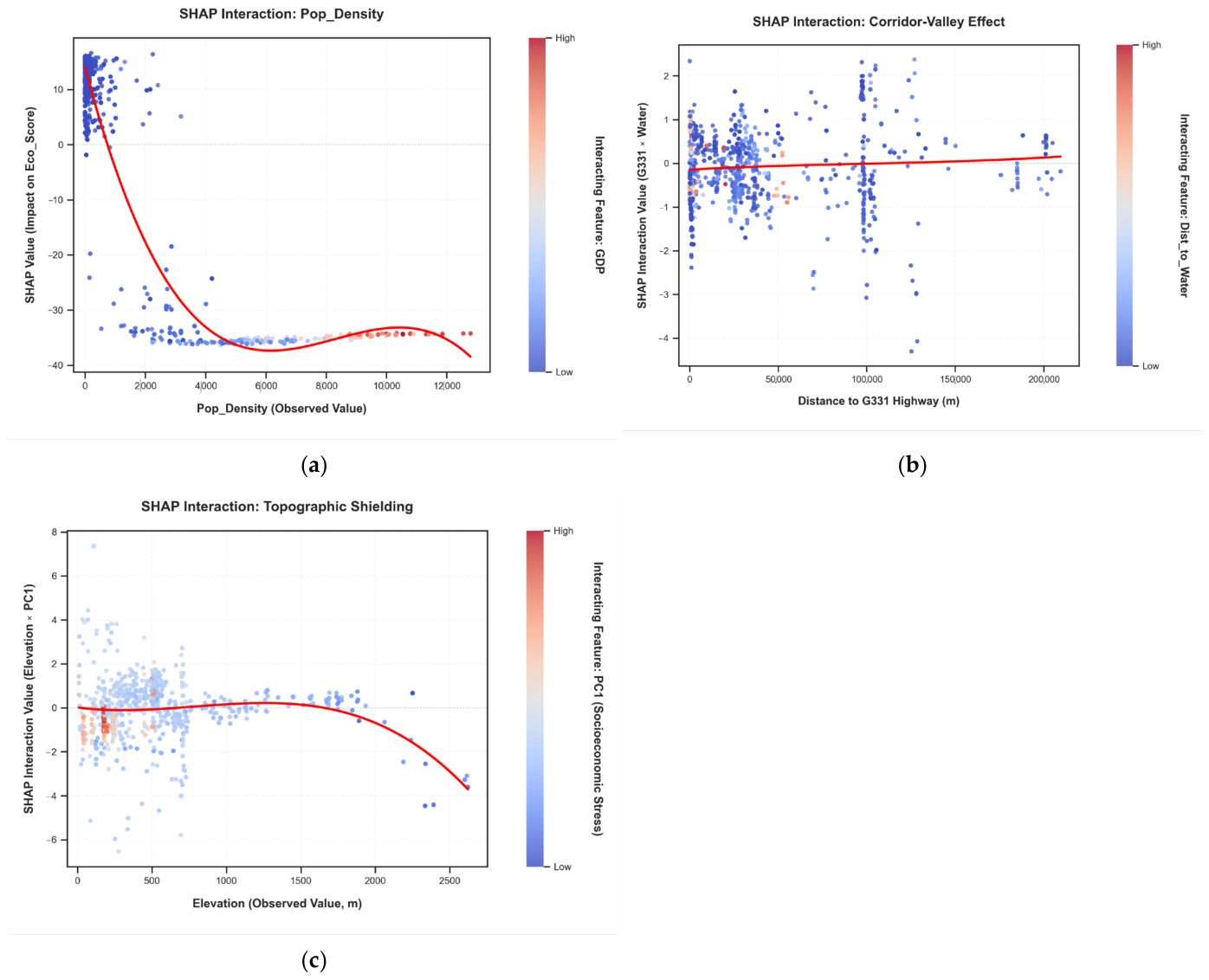
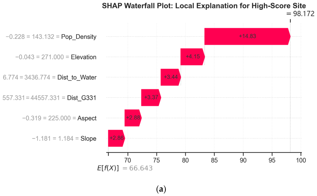
Sustainability 18 06631 g0a1
Table A1. Sensitivity analysis of Eco_Score weighting schemes.
Weighting SchemePearson r with BaselineSpearman r with BaselineR2 MeanRMSETop SHAP Component
Conservative0.7950.4990.8888.808PC1
Disturbance-sensitive0.7500.5050.87612.718PC1

References

  1. Tyagi, S. Impact of tourism sustainability on regional development: A systematic literature review. J. Policy Res. Tour. Leis. Events 2024, 16, 290–309. [Google Scholar] [CrossRef]
  2. Qiu, X.; Jin, M.; Zheng, Q. Association between land-use mix and the diversity of urban park activities: Evidence from six districts of Guangzhou, China. Int. J. Innov. Comput. Inf. Control 2026, 22, 283–300. [Google Scholar]
  3. Wang, T.; Yang, Z.; Han, F.; Yu, J.; Ma, X.; Han, J. Assessment of tourism socio-ecological system resilience in arid areas: A case study of Xinjiang, China. Ecol. Indic. 2024, 159, 111748. [Google Scholar] [CrossRef]
  4. Epifani, F. Sustainable governance of tourism-based social–ecological systems: Developing a synthetic index (STAI). Sustainability 2023, 15, 15967. [Google Scholar] [CrossRef]
  5. Huo, D.; Zheng, Q.; Pei, L. Investigating the characteristics of urban comprehensive hospitals from a supply–demand balance perspective: A case study of three districts in Shenzhen based on Multi-Source Data. Sustainability 2023, 15, 3327. [Google Scholar]
  6. López-Vera, B.M.; Pelegrín-Entenza, N. Methodological Reflection on Sustainable Tourism in Protected Natural Areas. Sustainability 2025, 17, 6558. [Google Scholar] [CrossRef]
  7. Vurnek, M.; Brozinčević, A.; Čulinović, K.; Novosel, A. Challenges in the Management of Plitvice Lakes National Park, Republic of Croatia. In National Parks—Management and Conservation; Suratman, M.N., Ed.; IntechOpen: London, UK, 2018; pp. 55–72. [Google Scholar] [CrossRef]
  8. Candia, S.; Pirlone, F.; Spadaro, I. Integrating the Carrying Capacity Methodology into Tourism Strategic Plans: A Sustainable Approach to Tourism. Int. J. Sustain. Dev. Plan. 2020, 15, 393–401. [Google Scholar] [CrossRef]
  9. Koh, E.; Fakfare, P. Overcoming “over-tourism”: The closure of Maya Bay. Int. J. Tour. Cities 2020, 6, 279–296. [Google Scholar] [CrossRef]
  10. Byers, A.C.; Gustafsson, T.; Shrestha, M.; Chhetri, N. A sustainable solid waste management plan for Sagarmatha (Mt Everest) National Park and Buffer Zone, Nepal. Mt. Res. Dev. 2020, 40, A1–A9. [Google Scholar] [CrossRef]
  11. Jin, M.; Zheng, Q.; Shao, Y.; Tian, Y.; Yu, J.; Zhang, Y. Spatial Optimization of Urban-Scale Sponge Structures and Functional Areas Using an Integrated Framework Based on a Hydrodynamic Model and GIS Technique. Water 2026, 18, 262. [Google Scholar] [CrossRef]
  12. Monz, C.A.; Cole, D.N.; Leung, Y.F.; Marion, J.L. Sustaining visitor use in protected areas: Future opportunities in recreation ecology research based on the USA experience. Environ. Manag. 2010, 45, 551–562. [Google Scholar] [CrossRef] [PubMed]
  13. Qu, L.; Hai, R.; Liang, K.; Zheng, Q.; Jin, M. Multi-Scale Attribution of Land Surface Temperature Driving Mechanisms in a Cold Region City: A Study on Spatial Non-Stationarity and Nonlinearity Based on XGBoost-SHAP. Sustainability 2026, 18, 4451. [Google Scholar]
  14. Yang, L.; Zhang, Y.; Zheng, Q.; Jin, M. Spatial heterogeneity and drivers of social vulnerability in chinese floodplains: A PCA-MGWR approach. Sci. Rep. 2026, 16, 16172. [Google Scholar] [CrossRef] [PubMed]
  15. Cork, N.A.; Fisher, R.S.; Strong, N.; Ferranti, E.J.S.; Quinn, A.D. A systematic review of factors influencing habitat connectivity and biodiversity along road and rail routes in temperate zones. Front. Environ. Sci. 2024, 12, 1369072. [Google Scholar] [CrossRef]
  16. Geneletti, D. A GIS-based decision support system to identify nature conservation priorities in an alpine valley. Land Use Policy 2004, 21, 149–160. [Google Scholar] [CrossRef]
  17. Dormann, C.F.; McPherson, J.M.; Araújo, M.B.; Bivand, R.; Bolliger, J.; Carl, G.; Davies, R.G.; Hirzel, A.; Jetz, W.; Kissling, W.D.; et al. Methods to account for spatial autocorrelation in the analysis of species distributional data: A review. Ecography 2007, 30, 609–628. [Google Scholar] [CrossRef]
  18. Friedman, J.H. Greedy function approximation: A gradient boosting machine. Ann. Stat. 2001, 29, 1189–1232. [Google Scholar] [CrossRef]
  19. Ribeiro, M.T.; Singh, S.; Guestrin, C. “Why should I trust you?”: Explaining the predictions of any classifier. In Proceedings of the 22nd ACM SIGKDD International Conference on Knowledge Discovery and Data Mining; Association for Computing Machinery: New York, NY, USA, 2016; pp. 1135–1144. [Google Scholar] [CrossRef]
  20. Lundberg, S.M.; Erion, G.; Chen, H.; DeGrave, A.; Prutkin, J.M.; Nair, B.; Katz, R.; Himmelfarb, J.; Bansal, N.; Lee, S.-I. From local explanations to global understanding with explainable AI for trees. Nat. Mach. Intell. 2020, 2, 56–67. [Google Scholar] [CrossRef] [PubMed]
  21. Kim, M.; Kim, D.; Jin, D.; Kim, G. Application of explainable artificial intelligence (XAI) in urban growth modeling: A case study of Seoul Metropolitan Area, Korea. Land 2023, 12, 420. [Google Scholar] [CrossRef]
  22. Breshanaj, M. From black box to insights: XGBoost and SHAP for interpretable tourism forecasting in Albania. Acad. J. Bus. Adm. Law Soc. Sci. 2025, 11, 44–56. [Google Scholar] [CrossRef]
  23. Du, P.; Huai, H.; Wu, X.; Wang, H.; Liu, W.; Tang, X. Using XGBoost-SHAP for understanding the ecosystem services trade-off effects and driving mechanisms in ecologically fragile areas. Front. Plant Sci. 2025, 16, 1552818. [Google Scholar] [CrossRef] [PubMed]
  24. Ye, S.; Li, Z.; Xi, J. A model for estimating the tourism carrying capacity of a tourism corridor: A case study of the Qinghai–Tibet Plateau. Sustainability 2024, 16, 5466. [Google Scholar] [CrossRef]
  25. Yu, K.; Gao, H. Sustainable development, eco-tourism carrying capacity and fuzzy algorithm: A study on Kanas in Belt and Road. Sci. Rep. 2023, 13, 16789. [Google Scholar] [CrossRef] [PubMed]
  26. Hjalager, A.-M. Land-use conflicts in coastal tourism and the quest for governance innovations. Land Use Policy 2020, 94, 104566. [Google Scholar] [CrossRef]
  27. Deb, K.; Pratap, A.; Agarwal, S.; Meyarivan, T. A fast and elitist multiobjective genetic algorithm: NSGA-II. IEEE Trans. Evol. Comput. 2002, 6, 182–197. [Google Scholar] [CrossRef]
  28. Shaygan, M.; Alimohammadi, A.; Mansourian, A.; Govara, Z.S.; Kalami, S.M. Spatial multi-objective optimization approach for land use allocation using NSGA-II. IEEE J. Sel. Top. Appl. Earth Obs. Remote Sens. 2014, 7, 873–883. [Google Scholar] [CrossRef]
  29. García, G.A.; Rosas, E.P.; García-Ferrer, A.; Barrios, P.M. Multi-objective spatial optimization: Sustainable land use allocation at sub-regional scale. Sustainability 2017, 9, 927. [Google Scholar] [CrossRef]
  30. Chen, T.; Guestrin, C. XGBoost: A Scalable Tree Boosting System. In Proceedings of the 22nd ACM SIGKDD International Conference on Knowledge Discovery and Data Mining, San Francisco, CA, USA, 13–17 August 2016. [Google Scholar] [CrossRef]
  31. Lundberg, S.M.; Lee, S.-I. A Unified Approach to Interpreting Model Predictions. In Advances in Neural Information Processing Systems 30; Curran Associates, Inc.: Red Hook, NY, USA, 2017. [Google Scholar] [CrossRef]
  32. Zhang, Q.; Li, H. MOEA/D: A multiobjective evolutionary algorithm based on decomposition. IEEE Trans. Evol. Comput. 2007, 11, 712–731. [Google Scholar] [CrossRef]
  33. Costanza, R.; d’Arge, R.; de Groot, R.; Farber, S.; Grasso, M.; Hannon, B.; Limburg, K.; Naeem, S.; O’Neill, R.V.; Paruelo, J.; et al. The value of the world’s ecosystem services and natural capital. Nature 1997, 387, 253–260. [Google Scholar] [CrossRef]
  34. Xie, G.D.; Zhen, L.; Lu, C.X.; Xiao, Y.; Li, W.H. Applying value transfer method for eco-service valuation in China. J. Resour. Ecol. 2010, 1, 51–59. [Google Scholar]
  35. Xie, G.; Zhang, C.; Zhen, L.; Zhang, L. Dynamic changes in the value of China’s ecosystem services. Ecosyst. Serv. 2017, 26, 146–154. [Google Scholar] [CrossRef]
  36. Liu, H.; Hai, R.; Zheng, Q.; Jin, M. Quantifying the Spatial Antagonism Between Urban Morphology and Ecological Infrastructure on Land Surface Temperature: An Explainable Machine Learning Approach with Spatial Lags. Buildings 2026, 16, 991. [Google Scholar] [CrossRef]
  37. Zhang, N.; Zheng, Q.; Jin, M.; Qiao, P. Unveiling the Non-Linear Associations Between 3D Building Morphology and Urban Thermal Environments: A Data-Driven Analytical Framework. Buildings 2026, 16, 2257. [Google Scholar] [CrossRef]
Figure 1. Conceptual framework for sustainability-oriented tourism corridor governance. The model conceptualizes a tourism corridor as a coupled social–ecological system in which socioeconomic pressure, accessibility structure, ecological vulnerability, and topographic background interact to shape spatial governance outcomes. Socioeconomic pressure and accessibility factors transmit development intensity across the corridor, ecological vulnerability reflects the sensitivity of landscape units, and topographic conditions may either amplify exposure or provide refuge effects. Explainable AI serves as an interpretive bridge that identifies non-linear thresholds, local mechanisms, and interaction effects, while evolutionary optimization translates these diagnostic insights into alternative governance scenarios.
Sustainability 18 06631 g001
Figure 2. Location map of the study area: (a) the geographical location of Jilin Province in China; and (b) the administrative division of Yanbian Prefecture alongside the specific scope of the study area.
Sustainability 18 06631 g002
Figure 3. The operational analytical workflow.
Sustainability 18 06631 g003
Figure 4. Spatial distribution of the multi-source dataset used in this study at 500 m grid resolution: (a) land-use/land-cover change data (LUCC); (b) digital elevation model (DEM); (c) topographic slope; (d) topographic aspect; (e) distance to the G331 National Highway (Dist_G331); (f) population density (POP); (g) gross domestic product (GDP); and (h) distance to water systems (Dist_Water).
Sustainability 18 06631 g004
Figure 5. Tourist Resource Points (POIs).
Sustainability 18 06631 g005
Figure 6. Distribution comparison of ecological quality scores (Eco_Score) across different spatial scales.
Sustainability 18 06631 g006
Figure 7. Identification of orthogonal environmental predictors using PCA. (a) Factor loadings heatmap decoding the physical semantics of extracted components, with PC1 dominated by socioeconomic pressures and subsequent PCs capturing topographic complexity; (b) Scree plot confirming the retention of core spatial variance above the 85% cumulative threshold.
Sustainability 18 06631 g007
Figure 8. Predictive performance evaluation and benchmark comparison of the machine learning models. (a) Benchmark comparison of Multiple Linear Regression (MLR), Random Forest (RF), and the optimized XGBoost model across the coefficient of determination (R2) and Root Mean Square Error (RMSE) metrics; (b) Validation scatter plot of the Bayesian-optimized XGBoost model, demonstrating high congruence between predicted and observed ecological scores along the 1:1 reference line.
Sustainability 18 06631 g008
Figure 9. Evaluation of spatial robustness and data leakage under spatial autocorrelation.
Sustainability 18 06631 g009
Figure 10. Global feature importance.
Sustainability 18 06631 g010
Figure 11. The SHAP summary plot.
Sustainability 18 06631 g011
Figure 12. SHAP dependence plots illustrating the non-linear responses of ecological quality to key environmental predictors: (a) Population Density, (b) Distance to G331 National Highway, (c) Elevation, and (d) Distance to Water Systems. The red solid lines represent the fitted trend of SHAP values, while the color gradients denote the interaction effects between each primary predictor and secondary spatial variables (e.g., distance to the G331 highway). These plots identify critical thresholds and non-monotonic response patterns within the corridor.
Sustainability 18 06631 g012
Figure 13. SHAP interaction patterns illustrating second-order dependencies: (a) Interaction between Population Density and GDP, revealing the transition from synergistic to antagonistic effects; (b) The “Corridor-Valley Effect” showing the joint impact of distance to the G331 highway and distance to water systems; (c) “Topographic Shielding” effect showing the interaction between elevation and socioeconomic pressure (PC1). The color scale indicates the intensity of the interacting feature, and the red lines represent the smoothed trend of the interaction values.
Sustainability 18 06631 g013
Figure 14. SHAP waterfall plots for local interpretability: (a) A high-scoring site demonstrating the positive contribution of topographical stability and isolation from human infrastructure; (b) A low-scoring site highlighting the compounded ecological deficit driven by high population density and proximity to the G331 national highway. E[f(x)] represents the baseline expected value, and f(x) denotes the final predicted score for the specific spatial unit.
Sustainability 18 06631 g014aSustainability 18 06631 g014b
Figure 15. Pareto-optimal frontier of spatial multi-objective optimization. The blue points signify the non-dominated spatial configurations identified by the NSGA-II algorithm. Three representative scenarios are highlighted: Scenario A (Eco-Preservation), Scenario B (Compromise Balance at the Pareto elbow), and Scenario C (Economic Expansion). The horizontal axis represents the PC1-derived socioeconomic development potential, while the vertical axis denotes the optimized ecological quality score.
Sustainability 18 06631 g015
Figure 16. Multidimensional performance comparison of the three spatial governance scenarios: Eco-Preservation, Compromise Balance, and Socioeconomic Development. The radar chart visualizes the distinct trade-offs across five core evaluative axes: Ecological Quality, Socioeconomic Benefit, Development Intensity, Corridor Connectivity, and Policy Constraint. Scenario B demonstrates a strategic equilibrium, maximizing socioeconomic benefits while adhering to critical ecological stability thresholds. All dimensions are standardized on a scale of 0 to 100 for benchmark comparison.
Sustainability 18 06631 g016
Table 1. Data sources, temporal coverage, spatial resolution, and harmonization procedures.
CategoryVariable NameMeaning and UnitSource of DataTemporal Coverage/Acquisition YearOriginal Resolution/Update Frequency/Harmonization
Dependent variableEco_ScoreEvaluation score of ecological quality of tourism resource sites; unitless indexEcological value scoring based on land use and land cover change data (LUCC)2020 LUCC dataset used in this studyOriginal LUCC raster resolution: 30 m; resampled to 500 m × 500 m analytical grid
Topographic backgroundElevationVertical height (m)SRTM 1 Arc-Second Global/ASTER GDEM Digital Elevation ModelSRTM mission acquisition period; treated as a static topographic baseline1 arc-second, approximately 30 m; no regular annual update; resampled to the 500 m × 500 m analytical grid
SlopeSurface unit inclination degree (°)Derived from DEMStatic topographic baseline; derived from DEMDerived from 30 m DEM; resampled to 500 m × 500 m analytical grid
AspectSlope orientation (°)Derived from DEMStatic topographic baseline; derived from DEMDerived from 30 m DEM; resampled to 500 m × 500 m analytical grid
Socioeconomic pressure Pop_DensityPopulation density (people/km2)WorldPop Global Project Population Data, University of SouthamptonDataset temporal coverage: 2015–2030; version R2025A v1; annual layer used in this study: 2025Annual gridded population dataset; 30 arc-seconds, approximately 1 km near the equator; resampled to the 500 m × 500 m analytical grid
GDPEconomic development level (10,000 yuan/km2)China’s Annual Spatial Grid GDP Dataset, Resource and Environment Science and Data Center2020 GDP grid used in this studyAnnual gridded GDP dataset; original resolution approximately 1 km; resampled to the 500 m × 500 m analytical grid
Spatial accessibilityDist_G331Euclidean distance from G331 National Road (m)Calculated based on OpenStreetMap road-network data from GeofabrikOSM extract as of 14 April 2026Vector road-network data; distance calculated and rasterized/resampled to 500 m × 500 m analytical grid
Dist_to_WaterDistance to the nearest water system (river/lake) (m)Calculated based on OpenStreetMap hydrographic data from GeofabrikOSM extract as of 14 April 2026Vector hydrographic data; distance calculated and rasterized/resampled to 500 m × 500 m analytical grid
Tourism-resource dataTourism resource points/POITourism-resource locations used for spatial joining and corridor modellingPOI/tourism-resource dataset collected by the authorsCollected on 19 January 2025Point data; 1468 valid tourism-resource records after preprocessing
Table 2. EQI Scoring Matrix.
LULC CategoryEcological Quality Score (Si)Weighting Basis/Description of Ecological Functions (Rationale)
Forest1.0The highest levels of biodiversity, carbon sequestration capacity and water conservation capabilities
Water0.9Key microclimate regulation, water cycle and habitat support
Grassland0.7Strong carbon sequestration capacity, but biomass is lower than that of forest land
Cropland0.4Has ecological productivity but is severely affected by human activities.
Unused Land0.1Lower habitat service capacity, high ecological sensitivity
Built-up Land0.1Extremely low ecological carrying capacity, highly artificialized interference from human activities
Table 3. Optimal hyperparameters for the XGBoost model.
HyperparameterDescriptionOptimal Value
n_estimatorsTotal number of gradient boosted trees to be built during training.1390
learning_rateStep size shrinkage used in update to prevent overfitting.0.0332
max_depthMaximum depth of a tree; controls the complexity of the model.6
subsampleThe ratio of the training instances randomly sampled for each tree.0.618992
colsample_bytreeThe ratio of features randomly sampled for each tree construction.0.816483
reg_alpha (α)L1 regularization term on weights to increase model sparsity.0.001741
reg_lambda (λ)L2 regularization term on weights to reduce model overfitting.5.5010
Table 4. Comparison of alternative multi-criteria optimization methods for corridor governance.
MethodMain AdvantageMain Limitation for This StudySuitability
Weighted-sum optimizationSimple and transparent; easy to implementRequires predefined weights; may obscure trade-offs; may miss non-convex Pareto solutionsSuitable for single-preference decision-making, but less suitable for exploring full trade-off structures
AHP-based evaluationIncorporates expert judgement; useful for indicator weightingStrongly dependent on subjective pairwise comparisons; does not automatically generate spatial configurationsUseful for preliminary weighting, but insufficient for spatial optimization
TOPSISRanks predefined alternatives according to distance from ideal and negative-ideal solutionsRequires a fixed set of alternatives; does not produce a Pareto frontierUseful for post-optimization scenario ranking, but not for generating scenarios
MOPSOCan search multi-objective solution spaces; flexible for non-linear problemsMay require additional parameter tuning to maintain diversity and avoid premature convergencePotential alternative, but not selected as the primary algorithm
NSGA-IIGenerates non-dominated Pareto solutions; preserves solution diversity through crowding distance; suitable for conflicting objectivesComputationally more complex; results still depend on objective functions and constraintsMost suitable for this study because it reveals the ecological–socioeconomic trade-off frontier and supports scenario-based governance
Disclaimer/Publisher’s Note: The statements, opinions and data contained in all publications are solely those of the individual author(s) and contributor(s) and not of MDPI and/or the editor(s). MDPI and/or the editor(s) disclaim responsibility for any injury to people or property resulting from any ideas, methods, instructions or products referred to in the content.