Urban Waterlogging Risk Assessment Based on the Dynamic Response of Surface–Underground Transportation Networks

Abstract

In order to improve the assessment of the dynamic risk of urban waterlogging, this study addresses the limitations of existing methods in capturing the responses of surface roads and subway systems to inundation, as well as the resulting spatiotemporal risks. Using the Hanyang District in Wuhan as a case study, the research proposes a framework for assessing urban waterlogging risks based on the dynamic inundation responses of surface and underground transport systems under various rainfall scenarios. The waterlogging process is simulated using seven representative rainfall scenarios with a hydrodynamic model that integrates a one-dimensional pipe network, a two-dimensional surface overland flow model, and a generalized underground space model. A coupled road–subway transportation network is developed to analyze traffic capacity degradation, path redistribution, and cascading failures caused by waterlogging disturbances. Quantified dynamic response indicators are integrated into the H-E-V-C framework to assess dynamic urban waterlogging risk. The results indicate that direct failure caused by water accumulation is typically the primary catalyst for extensive degradation of the transportation network, while the expansion of congestion and localized overload failures further exacerbate cascading effects. Different rainfall patterns influence not only peak risk but also the duration and spatial development of high-risk areas. Incorporating the dynamic response of the transport system enables a more accurate assessment of the degradation of emergency accessibility and the ongoing accumulation of localized high-risk areas. These findings highlight the importance of dynamic risk assessment in identifying time-varying urban vulnerabilities and supporting the planning of sustainable urban drainage, traffic management, and phased early warning systems.

1. Introduction

Urban rainstorms and flood disasters have become increasingly common due to the combined effects of global climate change and rapid urbanization, posing greater risks to urban safety and socioeconomic stability. Human-induced heat island and rain island effects further exacerbate these hazards, often amplifying cascading impacts, increasing casualties, and causing significant economic losses. For example, the extraordinary flood that affected the Haihe River Basin in July 2023 disrupted multiple cities, while the Zhengzhou “7.20” extreme rainstorm event in 2021 caused severe casualties and significant direct economic losses. In this context, urban flood risk assessment has become an important component of contemporary disaster prevention and mitigation research. Specifically, urban waterlogging risk assessment serves as a foundation for understanding risk formation, identifying spatial variations, and supporting urban drainage planning, emergency management, and the development of resilient cities.

Traditional urban waterlogging risk assessments have primarily concentrated on hazard-based or static risk identification methods. Early studies often relied on the H-V framework, in which risk was understood as the combined effect of external hazard intensity and the vulnerability of affected elements. Although this framework is relatively simple and well-suited for rapid assessment under limited data conditions, it tends to blur the distinction between exposure and vulnerability. As disaster risk concepts have gradually become standardized, urban waterlogging risk assessment has evolved toward multidimensional frameworks, exemplified by the H-E-V and H-E-V-C models [1,2]. In these frameworks, hazard is typically defined by hydrodynamic variables such as inundation depth, extent, duration, flow velocity, and overflow intensity. Exposure is defined as the distribution of affected elements, including the population, buildings, roads, subway stations, and critical facilities. Vulnerability refers to the susceptibility of these elements to functional impairment or loss, while capacity denotes the urban system’s ability to resist, absorb, recover from, and adapt to waterlogging disturbances. Based on the H-E-V framework, Zhang et al. (2019) summarized research progress in urban flood risk assessment [3], and Huang et al. (2020) further reviewed the development of urban flood-disaster research from the perspectives of risk analysis and zoning methods [4].

With the development of risk-assessment theory, increasing attention has been paid not only to spatial differences in flood hazard but also to the temporal evolution of risk during the disaster process. Recent studies have increasingly incorporated human activity patterns and event processes into traditional H-E-V-based assessment frameworks, thereby promoting the development of dynamic risk assessment. Lazzarin et al. (2022) emphasized that flood losses depend not only on the maximum hazard value, but also on the temporal variation in hazard and exposure [5]. Han et al. (2024) developed an integrated urban flood risk assessment framework combining Representative Concentration Pathways (RCP) and Shared Socioeconomic Pathways (SSP) scenarios, demonstrating that static inundation results alone are no longer sufficient to meet the requirements of urban-scale risk identification [6]. He et al. (2025) further incorporated urban functional zoning and multi-period population activity data into the H-E-V framework, demonstrating that urban flood risk is closely related to temporal population flows and the intensity of activities within functional zones [7]. These studies suggest that dynamic risk assessment can better capture actual risk peaks in areas such as commercial districts, transportation hubs, and underground spaces than static assessment alone [8]. However, the practical application of such approaches still depends heavily on high-temporal-resolution data on rainfall, ponding, population activities, and traffic operations.

Among the urban systems affected by waterlogging, the transportation system is particularly important because it not only responds directly to flood disturbance but also strongly influences the continuity of urban services. The urban transportation system includes both the surface road network and the subway system [9]. During urban waterlogging, surface roads may experience reduced speeds, decreased capacity, interruptions at critical sections, and congestion propagation, while subway systems may face flooded entrances and exits, station closures, service suspensions, and passenger flow transfers [10]. More importantly, such disruptions can quickly spread from the facility level to the service level, leading to longer travel times to hospitals and shelters, decreased emergency dispatch efficiency, and diminished service capacity in certain areas [9,11]. Therefore, the response of the transportation system is not merely one of the consequences of flooding, but also an important mechanism through which local disturbance is translated into broader urban functional degradation.

This issue is central to dynamic urban waterlogging risk assessment. In cities with highly networked transportation systems and extensive underground development, merely determining whether affected elements lie within inundated areas is no longer sufficient to reflect actual functional damage. Indicators such as road traffic capacity, network connectivity, transportation accessibility, emergency response time, subway station inundation, underground space water ingress risk, and the extent of system functional degradation can more directly characterize the dynamic responses of affected elements during rainstorm events. Nevertheless, current studies have yet to fully integrate the surface road network and subway system into a unified framework for urban waterlogging risk assessment, nor have they consistently connected inundation processes, functional degradation, and service impacts to the spatial evolution of overall urban risk [12,13,14]. Consequently, the impact of transportation system disruptions on dynamic urban risk has not yet been adequately addressed.

This study develops a dynamic urban waterlogging risk assessment framework for Hanyang District, Wuhan. The framework links hydrodynamic simulation with the response of a coupled surface–underground transportation system under multiple rainfall-pattern scenarios. First, a coupled transportation network integrating the surface road system and the subway system is constructed to simulate traffic-load redistribution and cascading failures under flood disturbance. Second, dynamic indicators, including road load distribution, emergency response time, and non-overloaded pipe-network density, are incorporated into the H-E-V-C framework to strengthen the representation of functional degradation during disasters. Third, differences in transportation-system response and risk evolution under multiple rainfall-pattern scenarios are compared to identify the pace of risk expansion and the spatial concentration of high-risk areas.

2. Materials and Methods

2.1. Study Area

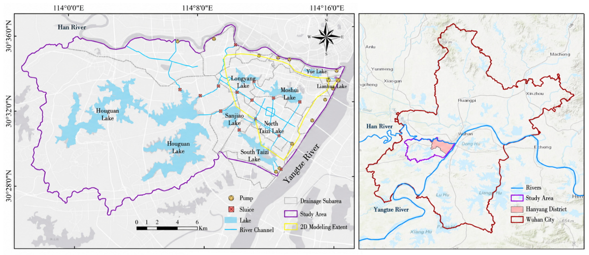
Wuhan is characterized by a network of crisscrossing rivers, interconnected harbors and canals, and widely distributed lakes and reservoirs. Its water-area ratio is the highest among provincial capitals in China. The urban center of Wuhan is divided by the Yangtze and Han Rivers into three major districts: Hankou, Hanyang, and Wuchang. The central urban area is low-lying and densely populated, featuring numerous lakes and ponds. During the flood season, elevated water levels in the outer rivers make drainage heavily dependent on pumping stations. The water system in Hanyang District includes six lakes—Houguan Lake, Longyang Lake, Moshui Lake, Triangle Lake, North Taizi Lake, and South Taizi Lake—which are interconnected through harbors and canals. Together with sluice pumps and a pipe-network drainage system, these lakes perform regional flood control and drainage functions. Rivers, canals, and lakes provide significant storage and regulation capacity, influencing the occurrence and development of urban waterlogging disasters. Based on topographic characteristics and the distribution of the drainage pipe network, this study currently excludes independent external drainage areas. It focuses solely on areas affected by lake storage and regulation under various scenarios of rainstorm-induced waterlogging. To balance computational demand and efficiency, separate one-dimensional and two-dimensional modeling domains were delineated. The study area is shown in Figure 1.

2.2. Principle of the Dynamic Response Model

Based on complex network theory, a multilayer transportation network model is constructed, integrating surface and underground transportation systems into a unified travel framework. The network comprises three layers: the travel network formed by origin-destination (OD) demand, the surface road network, and the subway network. Connectivity between surface and underground transportation is established by assigning OD demand to the nearest road nodes and creating virtual transfer edges. Using OD demand as the load and rainstorm-induced ponding as the disturbance, the model simulates the dynamic response of the transportation network.

2.2.1. Rainfall-Ponding Disturbance Scenario Settings

According to the China Meteorological Administration, a rainstorm is defined as intense, short-duration rainfall with a 24 h precipitation total of 50 mm or more. A rainfall pattern characterizes the temporal variation in rainstorm intensity over the course of an event, typically depicted by a hyetograph. Based on the temporal distribution of rainfall and the location of its peak, or rainfall center, former Soviet scholars proposed seven standard rainfall-pattern modes: front single-peak type, mid single-peak type, rear single-peak type, uniform type, mid double-peak type, front double-peak type, and rear double-peak type. These modes remain widely used as standard classifications in rainfall-pattern identification [15].

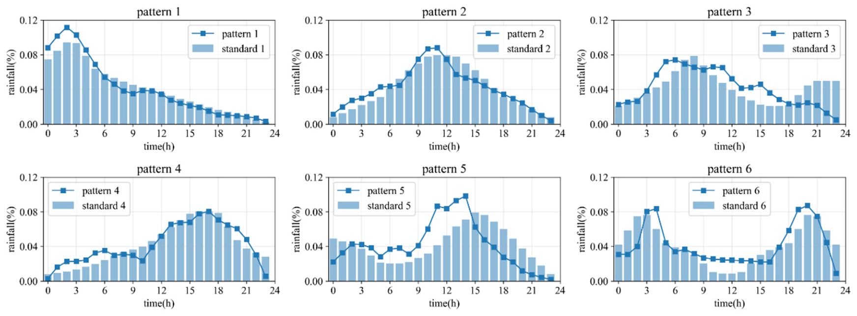
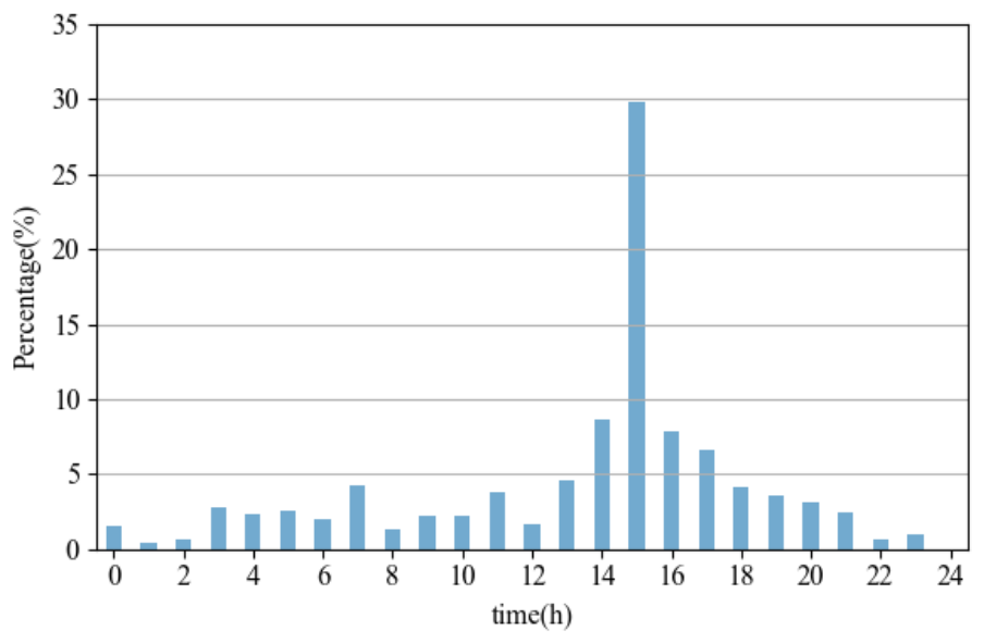
A fuzzy recognition method was used to analyze 53 observed rainfall events. Events with a similarity score above 0.7 to the seven standard rainfall patterns were classified accordingly using the nearest-principle criterion [16]. The results show no consistent rainfall pattern across the studied events, yielding six distinct rainfall-pattern modes. The rainfall processes within each pattern were averaged and interpolated to a 24 h scale to determine the proportional rainfall distribution, as shown in Figure 2. This study also considers design rainfall patterns. According to the local standard of Wuhan City, Wuhan City Rainfall Intensity Formula and Design Rainfall Pattern (DB4201/T 641-2020), the central urban area of Wuhan adopts a unified rainfall intensity formula. The corresponding rainfall distribution is shown in Figure 3. The 100-year return period rainfall depth is 321.51 mm.

This study employed five indicators to characterize the structural features of different rainfall patterns: maximum hourly rainfall intensity (P_max), temporal centroid of rainfall distribution (PCT), peak prominence index (PUP), asymmetry index (ASY), and hour of rainfall-peak occurrence (RP). P_max represents the maximum short-term rainfall intensity during a single event. PCT denotes the temporal centroid of rainfall distribution, with higher values indicating a greater concentration of rainfall in the later stages. PUP quantifies the prominence of the rainfall peak, with higher values indicating a more distinct peak structure. ASY captures the asymmetry in rainfall distribution before and after the peak, while RP indicates the timing of the dominant rainfall peak (see

Table 1. Characteristic parameters of different rainfall-pattern scenarios.

Variable	P_max	PCT	PUP	ASY	RP
1-Front-peak type	35.91	0.31	0.66	0.19	2
2-Mid-peak type	28.29	0.5	0.72	0.47	11
3-Front-peak uniform type	23.86	0.45	0.67	0.24	5
4-Rear-peak type	25.85	0.61	0.65	0.64	17
5-Double-peak rear-peak type	31.57	0.48	0.62	0.68	2 and 14
6-Double-peak uniform type	28	0.53	0.56	0.78	4 and 20
7-Design rainfall type	96.02	0.6	0.62	0.41	15

).

2.2.2. Principles of Hydrodynamic Model Computation

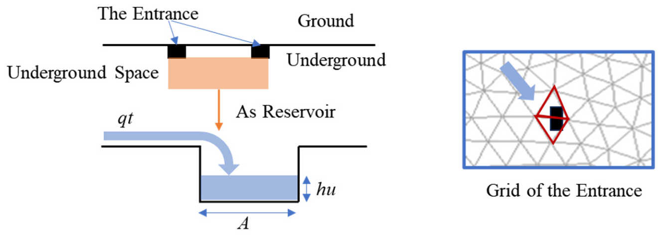
The Rainwater Management Model (SWMM) is used to simulate the one-dimensional flow process of water in pipes, while the two-dimensional shallow water equations are employed to model the surface water flow process. The calculation method adopts the finite volume method for the solution. However, the current hydrodynamic models lack mature calculation modules applicable to underground spaces. Previous studies have treated the entrances and exits of underground spaces as inspection wells [17] or utilized the distribution of buildings as an approximate proxy for the distribution of underground spaces [18]; however, these approaches are not fully applicable to large-scale inundation calculations involving multiple types of underground spaces. Therefore, this study conceptualizes underground spaces as water storage tanks, with their entrances and exits regarded as water exchange points connecting the two-dimensional hydrodynamic model and the generalized reservoir model. The “Simplified Reservoir Method” treats underground spaces as water storage units and employs the weir flow equation to calculate the inflow into these spaces, subsequently determining the inundation depth according to relevant formulas. The specific principles and methods for simplifying underground spaces, as well as the coupling connection methods, can be found in Reference [19]. The schematic diagram of the simplified calculation method is shown in Figure 4.

The reservoir method treats underground spaces as water-storage units, using Equation (1) to calculate inflow into the underground spaces and then computing inundation depth based on the corresponding equation.

$$q_t={\displaystyle {\sum }_{i=1}^{k}m{b}_i\sqrt{2g}{\left({\overline{h}}_i-z_i\right)}^{1.5}}$$

(1)

$${\overline{h}}_i={\displaystyle \frac{{\displaystyle {\sum }_{j=1}^n{h}_{ij}{A}_j}}{{\displaystyle {\sum }_{j=1}^n{A}_j}}}$$

(2)

$$h_u={\displaystyle \frac{{\displaystyle {\sum }_{t=1}^T{q}_t\Delta t}}{S}}\left(h_u<H_d\right)$$

(3)

where q_t represents the inflow through underground space entrances and exits at time t (m³/s); k denotes the number of entrances and exits; b_i denotes the width of entrance i (m); $\overline{h_i}$ denotes the average water depth of the n grid cells in which entrance i is located (m); h_ij and A_ij denote the water depth and area of grid cell j associated with entrance i, respectively (m and m²); z_i denotes the surface elevation of entrance or exit i (m); g is the gravitational acceleration (m/s²); m is the discharge coefficient, which is dimensionless and is typically set to 0.36; T is the total computation time (s); $\Delta t$ denotes the time step (s); S is the area of the underground space (m²); H_d is the height of the underground space (m); and h_u is the inundation depth within the underground space (m).

2.2.3. Nonlinear Load-Capacity Model of the Transportation Network

Surface roads are simplified and merged based on their topological structure, road type, grade, width, and related attributes. The road node closest to a subway station is designated as a transfer node, and transfer edges are constructed to integrate the surface and underground transportation systems. Initial attributes of transportation network edges are assigned according to road grade and type, as shown in

Table 2. Different settings for edge attributes of various types of transportation networks.

Type of Transportation Network	Type of Road	Initial Speed (km/h)	Initial Capacity (pcu/h)	Waiting Time (min)
Surface road network	Expressway	50	4000	1.0
	Main road	40	3000	0.8
	Secondary road	35	2500	0.5
Subway line network	Subway	60	4000	0
Connection layer	Virtual transfer edge	0.0013	4000	1.5

. To account for waiting times caused by traffic signals at intersections, the waiting time associated with transfers between surface roads and the subway is uniformly incorporated into the transfer edges. The speed of the transfer platform is set at walking speed, and its capacity is determined according to the corresponding subway platform to avoid the transfer platform affecting the route selection.

In the absence of actual traffic data, this paper employs an enhanced gravity model to estimate travel demand. This model is based on the theory of spatial interaction, which holds that the travel volume between regions is directly proportional to the population size at the starting point and the attractiveness at the destination, and inversely proportional to the travel impedance between the two.

$$o{d}_{ij}={\displaystyle \frac{P_i^{\alpha }{A}_j^{\gamma }}{{\rho }_{ij}^{\beta }}}$$

(4)

where P_i represents the population size of the starting area, A_j represents the comprehensive attractiveness of the destination area, and α and γ denote the population occurrence coefficient and facility attraction coefficient, respectively. ρ_ij denotes the travel impedance calculated from the road network, and β denotes the travel impedance attenuation parameter. The values of α, β, and γ are set to 0.5, 1.5, and 0.5, respectively.

To control the overall scale of traffic demand, the original OD matrix is normalized. This method can reasonably depict the spatial distribution characteristics of urban travel demand even with limited data.

OD demand is treated as the load on the road network system, while road carrying capacity is considered the system capacity. A nonlinear model is introduced to describe the behavioral evolution of road network components. The nonlinear relationship between load and capacity is defined as follows:

$$C_a^0=\left\{\begin{array}{ll}{L}_a^0+\alpha {\left(L_a^0\right)}^{\beta },\hfill & L_a^0>L_{a,0}\hfill \\ \left(1+\alpha \right)L_a^0,\hfill & L_a^0<L_{a,0}\hfill \end{array}\right.$$

(5)

where $C_a^0$ denotes the initial capacity of network component a; $L_a^0$ denotes the initial load; $L_{a,0}$ denotes the initial load under free-flow traffic conditions; and α and β are nonnegative adjustable parameters.

When the real-time load slightly exceeds capacity, a node or edge may become overloaded without complete failure, although its capacity begins to decrease. Therefore, a time-varying capacity update method based on a nonlinear load-capacity model is adopted to describe the relationship between capacity and load [20]. The capacity of network component a is defined as follows:

$$C_a^{t+1}=\left\{\begin{array}{ll}{C}_a^0{\displaystyle \frac{C_a^t}{L_a^t}},\hfill & L_a^t>C_a^t\hfill \\ C_a^t,\hfill & L_a^t\le C_a^t\hfill \end{array}\right.$$

(6)

where $C_a^0$ denotes the initial capacity, $L_a^t$ denotes the load, and $C_a^t$ denotes the capacity, respectively.

The BPR function is used to calculate free-flow travel time and traffic impedance for a road segment. In this study, it is employed to quantify changes in vehicle travel time, specifically.

$${\rho }_a^t={\rho }_a^0\left[1+\sigma {\left({\displaystyle \frac{L_a^t}{C_a^t}}\right)}^{\mu }\right]$$

(7)

where ${\rho }_a^t$ denotes vehicle travel time, ${\rho }_a^0$ denotes free-flow travel time, and $\sigma$ and $\mu$ denote saturation-related parameters, which are typically assigned values of 0.15 and 4, respectively. $\sigma$ and $\mu$ could be updated according to the different conditions [20].

When ponding occurs on a road, vehicle speed decreases. Once the vehicle speed falls below the design speed, the road’s traffic capacity is considered reduced [11,16]. Huang et al. (2023) summarized the relationship between ponding depth and vehicle speed, demonstrating a significant negative correlation between vehicle speed and rainfall-induced inundation [21]. Among the available models, Du et al. (2011) proposed a hyperbolic function based on statistical methods to represent speed attenuation; this model has been widely applied [22].

$$v={\displaystyle \frac{v_0}{2}}\tan \mathrm{h}\left({\displaystyle \frac{-x+a}{b}}\right)+{\displaystyle \frac{v_0}{2}}$$

(8)

where v denotes operating speed, v₀ denotes design speed (which varies by road type), x denotes ponding depth (cm), a is the median critical water depth at which vehicles stop, and b is the elastic attenuation coefficient, which reflects the rate of speed reduction as water depth increases and typically ranges from 3 to 5. A smaller coefficient indicates faster speed attenuation. Considering the similarities of the study area, a and b were set to 7.5 and 3, respectively, and 0.3 m was adopted as the critical threshold for road disruption [23,24].

If the traffic load exceeds the design capacity, the network edge is considered overloaded, resulting in a decline in its traffic efficiency. When the overload reaches a certain threshold, the edge may become impassable. Therefore, the state of network edge a is defined as follows:

$${\Omega }_a^{t+1}=\left\{\begin{array}{cc}2,\hfill & \delta -{\displaystyle \frac{L_a^t}{C_a^t}}\le 0\hfill \\ 0,\hfill & L_a^t\le C_a^t\hfill \\ 1,\hfill & L_a^t>C_a^{t}and\delta -{\displaystyle \frac{L_a^t}{C_a^t}}>0\hfill \end{array}\right.$$

(9)

where 0 indicates normal operation, 1 indicates congestion, 2 indicates failure, and the corresponding symbol denotes the failure threshold, which is greater than 1.

The failure threshold significantly influences the process of network risk diffusion and failure. When the failure threshold is low, the speed of risk diffusion increases, and the dynamic response time of network cascading failure decreases. As the failure threshold rises, the rate at which risk spreads to other nodes slows down. If the failure threshold is too high, it becomes difficult to capture the process of risk propagation. Based on parameter sensitivity analysis and relevant literature [20], this paper selects a failure threshold of 1.5 for subsequent analysis.

When an edge or node fails, its load is redistributed among the remaining available edges according to a specified proportion. In this study, the load of a failed node is allocated to neighboring nodes or edges, second-nearest neighbors, or nodes farther from the failed node based on a multivariate Gaussian distribution. The probability density function of the multivariate Gaussian distribution is defined as follows:

$$f\left(X\right)={\displaystyle \frac{e^{-\frac{1}{2}\left(X-{\mu }_X\right){\displaystyle {\sum }_{\mathrm{X}}^{-1}\left(X-{\mu }_X\right)}}}{{\left(2\pi \right)}^{\frac{r}{2}}{\left|Co{v}_X\right|}^{\frac{1}{2}}}}$$

(10)

where X denotes an r-dimensional random vector, f(X) denotes the probability density function of the multivariate random vector X; ${\mu }_X$ denotes the mean vector; Cov_X denotes the covariance matrix; |Cov_X| denotes the determinant of the covariance matrix; and ${\left(2\pi \right)}^{{\displaystyle \frac{r}{2}}}$ denotes a normalization factor.

To simulate the dynamic response of the transportation network under the influence of rainfall and water accumulation disturbances, the network load is modified to bring the system to a critical state. At this point, the ratio of the initial load to the capacity of surface roads is approximately 0.50, while that of the subway is 0.30. About 5% of the initial loads on surface roads exceed their capacity. When the failure threshold is set at 1.5, the network has not yet reached a failure state, indicating that the initial condition of the transportation network is reasonable and that there is some operational stress. This facilitates the spread of road congestion and the redistribution of traffic flow.

2.2.4. PSL-SUE Route Choice and Traffic Assignment Model

This study develops a path-size logit-based stochastic user equilibrium (PSL-SUE) traffic assignment model to characterize travelers’ multipath choice behavior in transportation networks and the feedback effect of traffic flow on network impedance. According to random utility theory, the model assumes that travelers between the same origin-destination pair do not consistently select a single shortest path; rather, they probabilistically choose among several feasible paths based on their overall utility. When path-choice outcomes align with the network impedance state, the system reaches stochastic user equilibrium.

Let the transportation network be denoted as G = (N, A), where N is the set of nodes, and A is the set of road segments. The travel demand for an OD pair (r, s) is represented by q(r, s), while the candidate path set for the same OD pair is denoted by K. The generalized impedance of a path is defined as follows:

$$I{M}_k={\displaystyle \sum _{a\in A}{\delta }_{a,k}}{\rho }_a+\gamma T_k-\eta M_k$$

(11)

where ${\rho }_a$ denotes the generalized impedance of a network component, ${\delta }_{a,k}$ denotes the path-link incidence variable, $T_k$ denotes the transfer-penalty term; $\gamma$ denotes the coefficient; $M_k$ denotes the subway-preference term; $\eta$ denotes the coefficient, respectively.

The depth of the water directly influences the travel speed on surface roads. Its impact on the underground transportation system is primarily evident in reduced efficiency at station entrances and exits, closures, and functional degradation resulting from damage to transfer facilities. The greater the total impedance of a route, the less likely travelers are to choose it. If a route involves more transfers, its overall impedance increases; conversely, if a route exhibits a stronger preference, its overall impedance correspondingly decreases.

To correct overlap among candidate paths, a path-size term is introduced:

$$P{S}_k={\displaystyle \sum _{a\in A}{\delta }_{a,k}}{\displaystyle \frac{l_a}{{Len}_k}}{\displaystyle \frac{1}{{\displaystyle \sum _{h\in K}{\delta }_{a,h}}}}$$

(12)

where l_a denotes link length or weight, and Len_k denotes the total length of the path k. The larger the path-size term, the more independent the path and the greater its effective attractiveness in the route-choice process.

Accordingly, the system utility of a path can be expressed as

$$V_k=-\theta L_k+\beta \ln \left({PS}_k\right)$$

(13)

where θ denotes the impedance-sensitivity coefficient, which represents travelers’ sensitivity to changes in path cost, and β denotes the path-size correction coefficient, which measures the strength of path independence in route choice. The greater the generalized path impedance, the lower the utility; the larger the path-size term, the more independent the path and, therefore, the higher its utility.

Within the stochastic user equilibrium framework, the PSL-SUE model incorporates a path-size correction term that both characterizes travelers’ probabilistic path-choice behavior among multiple feasible routes and effectively mitigates the correlation bias arising from path overlap. Simultaneously, it integrates the path-choice process with the flow-impedance feedback mechanism, thereby more accurately representing the traffic-flow redistribution characteristics of complex transportation networks under conditions of congestion or disruption. To assess the overall congestion level of the road network during extreme rainfall, this study employs the weighted congestion index (CI) as the evaluation metric. This indicator uses the actual traffic load of each road segment as the weight and calculates the weighted average of the link load-capacity ratio (L/C) to reflect the congestion state. For a road network containing multiple road segments, the weighted congestion index is defined as follows:

$$CI={\displaystyle \sum _{i=1}^n\frac{L_i^2}{C_i}}/{\displaystyle \sum _{i=1}^n{L}_i}$$

(14)

where L_i and C_i denote the actual traffic load and traffic capacity of road segment a, respectively.

2.3. Urban Waterlogging Risk Assessment Methodology

2.3.1. Dynamic Risk Assessment Framework for Urban Waterlogging

The Hazard-Exposure-Vulnerability-Capacity (H-E-V-C) framework is widely used for assessing urban waterlogging risk. It has gradually become an important analytical tool for comprehensively identifying urban flood risk. Its strength lies in systematically integrating key elements—hazard intensity, exposure characteristics of affected elements, damage sensitivity, and recovery capacity—to provide a unified basis for the comprehensive characterization and spatial analysis of urban waterlogging risk. Urban flood risk, however, is not static. It is a dynamic process closely tied to the real-time state of engineering systems and the temporal flows of pedestrians and vehicles. Accordingly, researchers have developed a dynamic H-E-V-C risk assessment system that accounts for the dynamic response processes of critical urban engineering systems. This system captures how actual risk peaks vary over time and how system functionality changes.

$$R_t=f\left(H_t,E_t,V,C_t\right)$$

(15)

where R_t denotes the waterlogging risk of an evaluation unit at time t; H_t, E_t, V, and C_t denote hazard, exposure, vulnerability, and capacity, respectively; and vulnerability is generally assumed to be time-invariant.

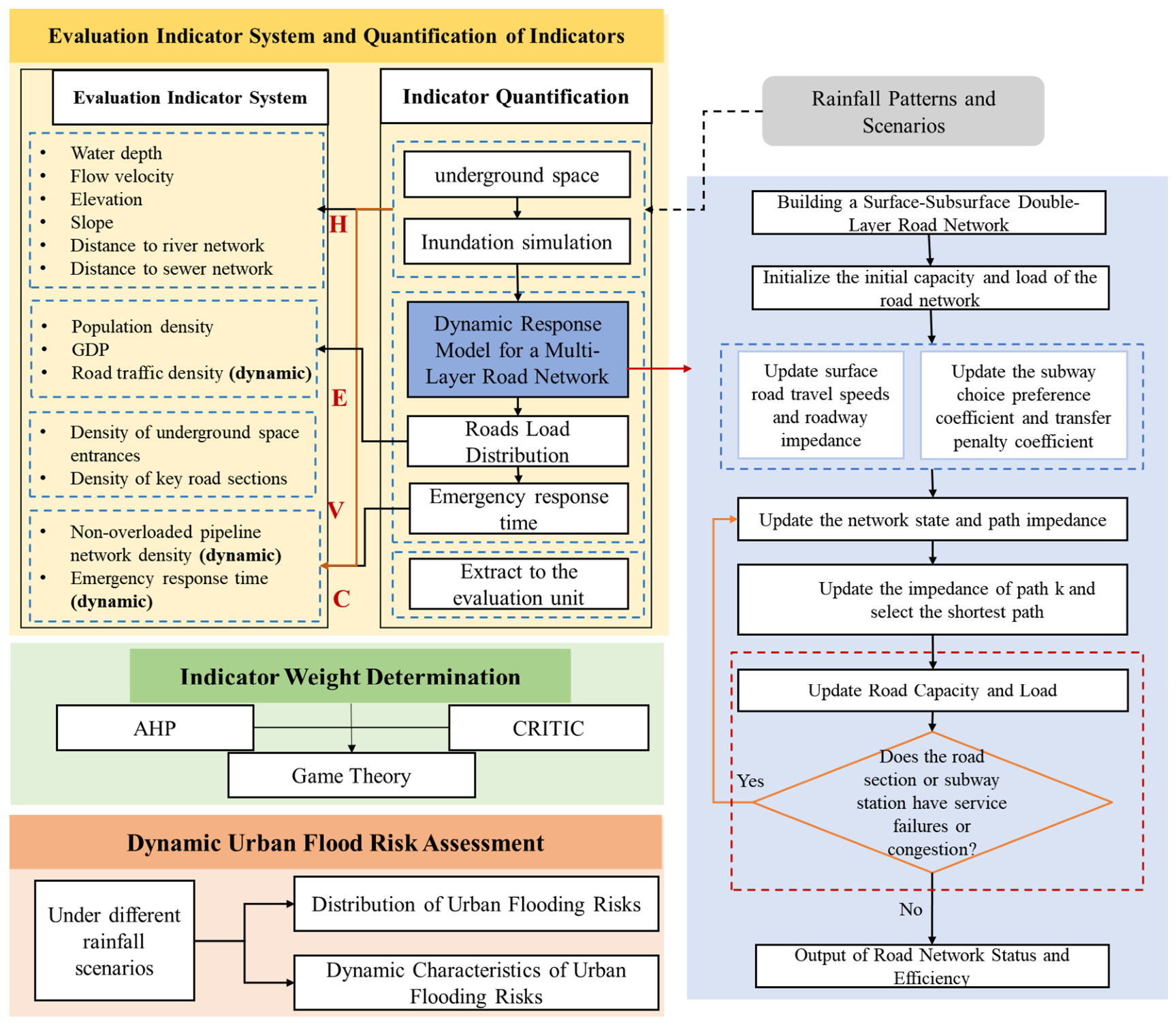
Scenario simulation combined with multi-criteria decision analysis (MCDA) is now a widely used approach to risk assessment. By revealing the true distribution of risk, this method standardizes evaluation indicators across different dimensions and units, integrates their respective weights, and thus improves objectivity and comprehensiveness. Accordingly, this study combines the dynamic H-E-V-C framework with the MCDA-based indicator evaluation method to quantitatively identify urban waterlogging risks from multi-scenario simulation results. Figure 5 illustrates the dynamic-response calculation for the road-network system under rainstorm scenarios.

2.3.2. Quantification Methods for Dynamic Response Indicators

The impact of urban waterlogging on the road system manifests not only through road inundation but also as a time-dependent deterioration of the network’s operational state and service capacity. Its impact on road traffic appears chiefly in two forms: a loss of traffic capacity and a reduction in spatial accessibility. At the same time, dynamic population movements substantially modify the spatiotemporal patterns of flood risk, while changes in road traffic capacity further affect accessibility to destinations such as emergency service facilities. Describing the road network’s response solely by road water depth or inundated length is therefore insufficient to capture the actual process of path-load redistribution and the decline in service connectivity under waterlogging scenarios. For this reason, the study selects road-load distribution and road accessibility as quantitative indicators of the dynamic road network response.

(1) Road-Load Distribution (Dynamic)

Road-load distribution captures how population activities and travel paths shift across the road network under waterlogging, quantified using a dynamic shortest-path assignment method constrained by flood conditions. Road accessibility measures the minimum travel time from a given unit to the nearest destination under concurrent ponding and congestion. Its relative loss rate indicates the decline in the network’s service capacity. The former reflects the network’s internal operational pressure; the latter, its capacity to support critical emergency services. Together, they serve as the primary indicators of the road network’s dynamic response to waterlogging.

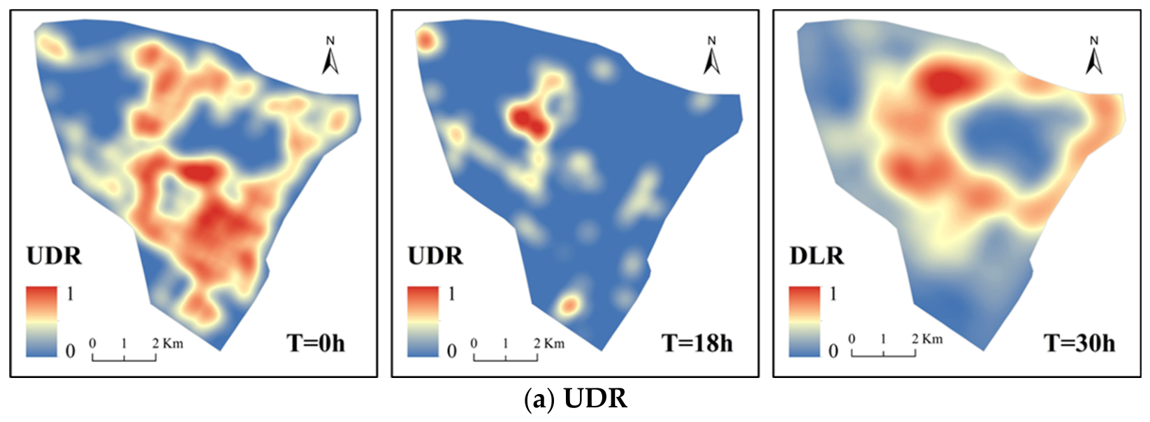
Road-load distribution represents the redistribution of internal operational pressure within the road network during waterlogging. When road segments become flooded, speeds drop, or certain routes are disrupted, residents’ travel and population movements are redirected along the remaining passable paths. This reassignment increases loads on some roads and intensifies local congestion. Static population density or static road density alone cannot capture changes in path-level carrying pressure during waterlogging events [25]. By projecting dynamic population and travel demand onto specific paths to form a road-load distribution, the operational state of the road network can be characterized more accurately. Since waterlogging affects only the entrances and exits of subway stations while underground operating speeds remain unaffected, this analysis focuses solely on the load distribution of surface roads.

If the set of dynamic travel demands at a given time is known, the load on a road segment can be expressed as:

$$L_{a,t}={\displaystyle \sum _{k\in {\Omega }_t}{q}_{k,t}}{\delta }_{a,k,t}$$

(16)

where $L_{a,t}$ denotes the dynamic load of road segment a at time t; $q_{k,t}$ denotes the intensity of the k-th travel demand or population-activity demand; and ${\delta }_{a,k,t}$ is the path-indicator variable, which equals 1 when road segment a lies on the shortest path for that demand under the current scenario and time, and 0 otherwise.

To eliminate the effects of road gradients and variations in traffic capacity, the current method for calculating the road load density of the assessment unit employs the road load rate as a weighting factor and is as follows:

$$L{R}_{a,t}={\displaystyle \frac{L_{a,t}}{C_{a,t}}}$$

(17)

$$DL{R}_{a,t}={\displaystyle \frac{1}{h}}{\displaystyle \sum _a^n{I}_a}K\left({\displaystyle \frac{d_i}{h}}\right)$$

(18)

where I_a denotes the standardized importance score of the road segment a, n is the number of road segments in the evaluation unit, d_i is the Euclidean distance between the evaluation unit and the center of the road segment, K( ) denotes the Gaussian kernel function, and h is the bandwidth controlling the smoothing range of the kernel function.

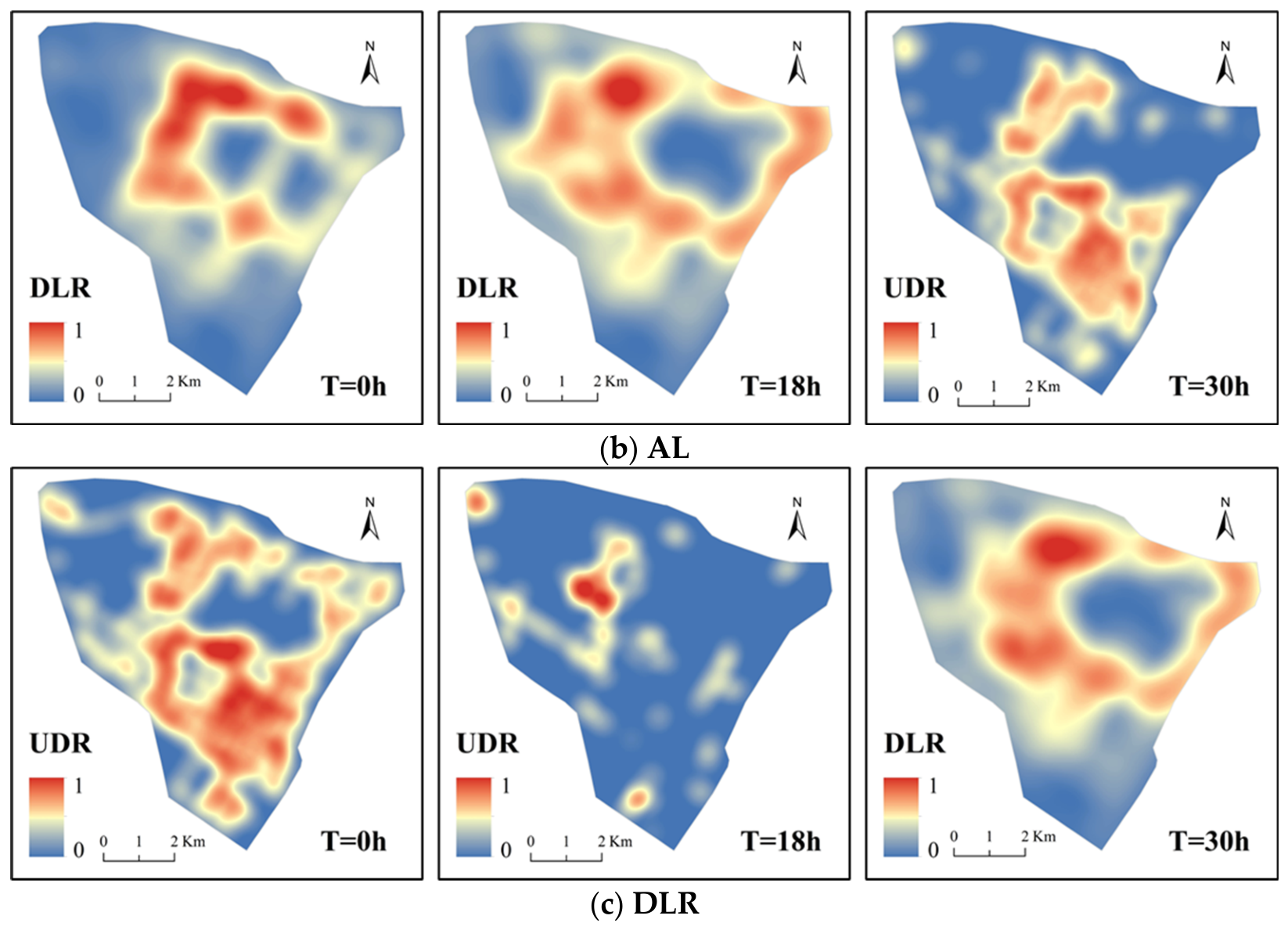
(2) Emergency response time (Dynamic)

Road accessibility represents the ability of the road network to support essential external services and indicates whether its service function is compromised under waterlogging conditions. It is not merely a product of traffic analysis but also an important variable that objectively characterizes changes in the service level of the road network during such conditions. Zang et al. (2024) found that accessibility to emergency services fluctuates significantly with variations in road traffic capacity [25]. In existing studies, road accessibility can serve as either an independent assessment outcome or a risk evaluation indicator [26].

The degradation of accessibility caused by waterlogging is described; the emergency response time is further specified as:

$$A{L}_{i,t}=\min \left(T_{i,t}^1,T_{i,t}^2,\cdots ,T_{i,t}^j\right)$$

(19)

where $A{L}_{i,t}$ denotes the emergency response time of a grid; P denotes the number of destination categories; $T_{i,t}^j$ denotes the minimum travel time from grid i under scenario t, and under no-waterlogging conditions, to the nearest destination of type j. The larger the value, the more significant the degradation of accessibility of that grid under the current scenario and time, and thus the higher the risk.

A multi-source Dijkstra algorithm is used to calculate the minimum travel time from each evaluation unit i at time t to the nearest destination. Hospitals and fire stations are considered the two types of emergency facilities, and the shortest travel time to each is calculated accordingly. If both types are reachable, the status is recorded as 0. During subsequent global normalization, all reachable travel times are normalized to the interval (0, 0.8). If one type is unreachable, the value is recorded as 0.9; if both types are unreachable, the value is recorded as 1.

(3) Non-Overloaded Pipe-Network Density (Dynamic)

Non-overloaded pipe-network density is a dynamic extension of static pipe-network density, used to quantify the length density of pipe networks that remain non-overloaded and retain residual drainage capacity under specific scenarios and timeframes. Unlike static pipe-network density, this metric reflects not only the presence of drainage facilities but also their current operational status. Changes in pipe-network structure and available drainage capacity significantly influence urban ponding response and the overall drainage efficiency of the system. Therefore, incorporating non-overloaded pipe-network density into capacity indicators provides a more realistic assessment of drainage support capability during disasters.

2.3.3. Combination Weighting Method

Urban waterlogging risk is characterized by multifactor coupling, pronounced spatial heterogeneity, and diverse indicator attributes. Relying solely on subjective weighting is therefore easily influenced by researchers’ experience and judgment, whereas using only objective weighting may overlook important links between indicators and disaster-causing mechanisms. Based on feature contributions from intelligent models, this study employs a game-theoretic CRITIC-AHP combination weighting method to determine indicator weights, thereby enhancing both the objectivity and interpretability of the weighting scheme.

The CRITIC method (Criteria Importance Through Intercriteria Correlation) determines the weight of an indicator based on both its contrast intensity and conflict. The AHP method (Analytic Hierarchy Process) derives weights by constructing a judgment matrix through expert pairwise comparisons of the relative importance of indicators, solving for the eigenvector, and assessing the rationality of the judgments using the consistency ratio (CR). The game-theoretic combination weighting method treats the two weight vectors as participants in a non-cooperative game and solves for the optimal linear combination coefficients under Nash equilibrium, minimizing the sum of squared deviations between the combined weight and each weight.

$$w_j^{\mathrm{final}}=\alpha w_j^{\mathrm{CRITIC}}+\left(1-\alpha \right)w_j^{\mathrm{AHP}}$$

(20)

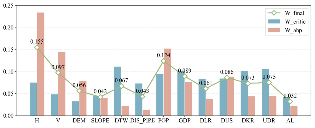
The final weights also satisfy the corresponding constraints, and their sum equals one. A higher risk value indicates a greater likelihood that the unit will be affected by urban waterlogging and experience functional disturbances under various rainfall pattern scenarios. Risk values are classified into five levels—low, relatively low, medium, relatively high, and high—using the natural breaks method. Global data are used for classification to facilitate comparison of risk differences among different schemes and at different times. The final weights of the risk assessment indicators are shown in Figure 6.

3. Model Development

3.1. Hydrodynamic Model Construction

The pipe network within the study area was simplified while retaining the main stormwater trunks. Consideration was given to rivers, interchanges, road intersections, and low-lying areas, and harbor channels were incorporated into the one-dimensional model. The pipe network was generalized into 2308 pipe segments, 2245 pipe-network nodes, 2301 subcatchments, and 5 outfalls, while lakes were treated as storage tanks functioning as regulation units. Coupled connections were established based on the spatial relationships between pipe-network nodes and grids, with the overflow process at pipe-network nodes serving as input for the corresponding two-dimensional grids. During the two-dimensional calculations, the corresponding water volume was added or subtracted to enable coupled pipe-network computation.

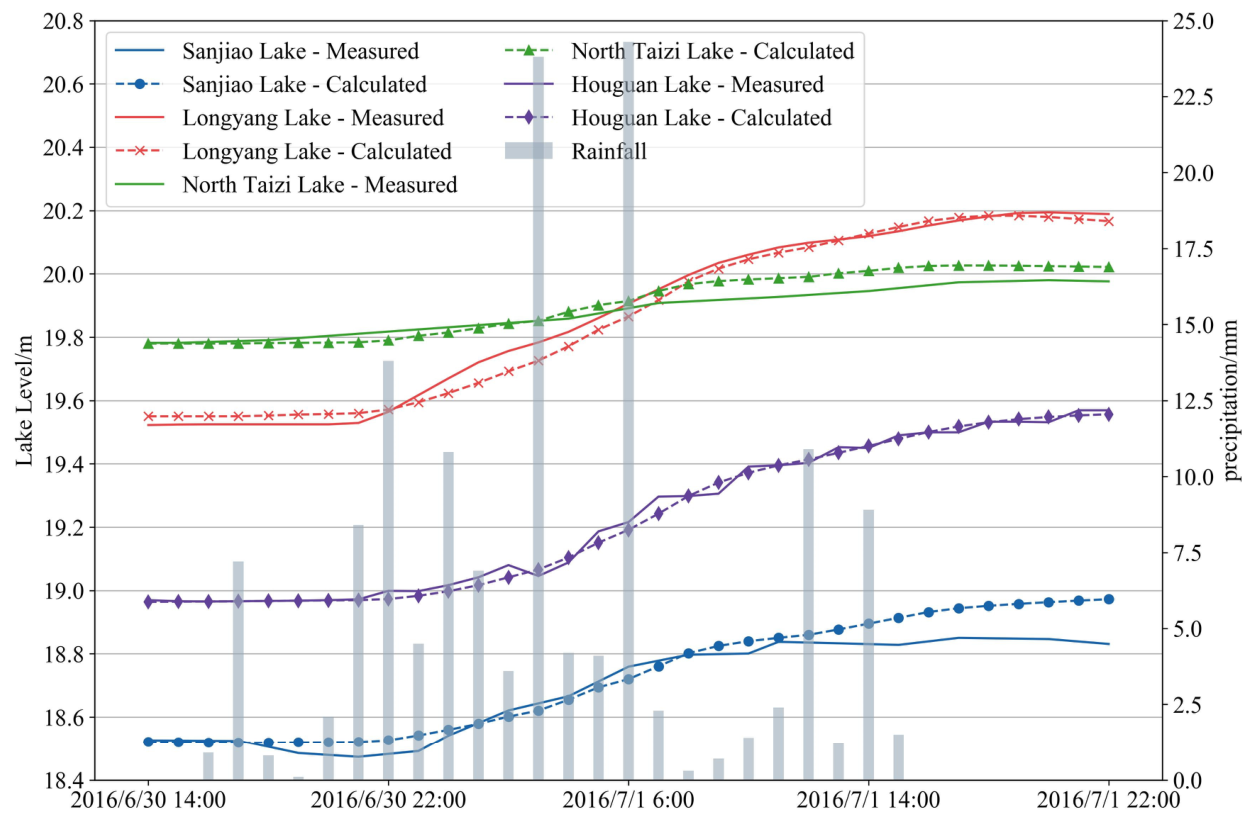
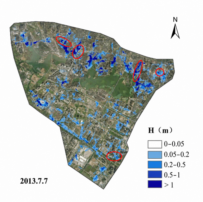
Owing to the absence of measured data for sluice and pump scheduling operations, the model validation process chiefly depended on the operating water levels of the respective sluices and pumps. Their scheduling principles and judgment, grounded in experience, are employed to simulate controlled operations. Rainfall data from 30 June 2016 to 14 July 2016 were used to calibrate and validate the one-dimensional model parameters. Based on the analysis and verification of the measured lake water level data, the one-dimensional model demonstrated a strong overall agreement between the simulated and observed values. The surface waterlogging conditions caused by the rainfall event on 7 July 2013 were used for secondary validation, with the results shown in Figure 7 and Figure 8.

3.2. Construction of the Risk Assessment Indicator System

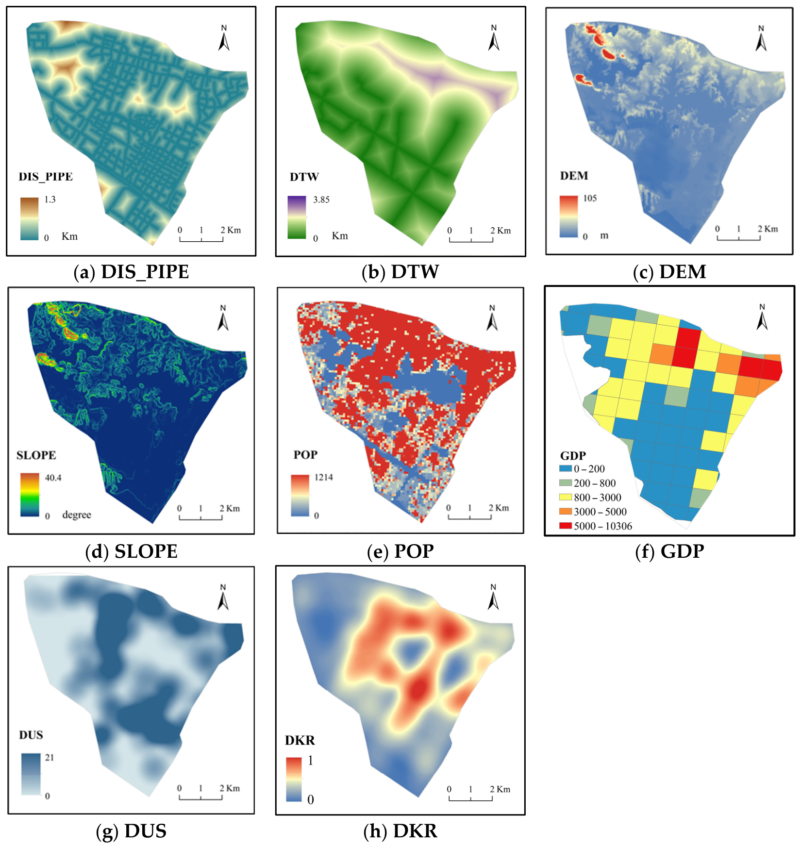
The selection of urban waterlogging risk assessment indicators directly influences the scientific rigor and interpretability of the final evaluation results. Therefore, the indicators should be representative, comprehensive, and easily obtainable. Hazard indicators primarily characterize ponding intensity and the intrinsic conditions that generate risk, including hazard-causing factors and hazard-forming conditions such as maximum inundation depth (H), maximum flow velocity (V), elevation (DEM), and slope (SLOPE). Exposure indicators reflect the extent to which populations, buildings, roads, key facilities, and assets are exposed under inundation scenarios. Vulnerability indicators describe the sensitivity of affected elements to damage, such as the density of underground space entrances (DUS). Capacity indicators represent the potential impact on urban operational functions and the response capability during urban waterlogging events. According to multicollinearity analysis, the variance inflation factor (VIF) for all indicators was below 10, indicating good independence among them. The classification, meaning, and positive or negative direction of each indicator are presented in

Table 3. Meaning and classification of risk assessment indicators.

Index	Type	Indicator	Indicator Meaning	Unit	Direction
1	H	Water Depth (H)	Flooding intensity of the evaluation unit	m	Positive
2	H	Flow Velocity (V)	Water impact and momentum intensity	m/s	Positive
3	H	Elevation DEM	Topographic elevation condition of the unit	m	Negative
4	H	Slope (SLOPE)	Slope drainage and runoff concentration efficiency	° or %	Negative
5	H	Distance to River Network (DTW)	Distance from the unit to the river network/natural drainage channel	m	Negative
6	H	Distance to Drainage System (DIS_PIPE)	Distance from the unit to the artificial drainage network/storm inlet	m	Negative
7	E	Population Density (POP)	Potentially affected population size within the unit	person/km2	Positive
8	E	GDP	Economic activity and asset value intensity within the unit	10,000 yuan/km2 or yuan/m2	Positive
9	E	Dynamic Road Load Density (DLR)	Intensity of dynamic population activities and travel demand on the road network at a given time	dimensionless	Positive
10	V	Underground Space Entrance Density (DUS)	Density of underground space entrances within the unit	entrances/km2	Positive
11	V	Critical Road Segment Density (DKR)	Kernel density of roads weighted by an importance score within the unit	m/km2 or km/km2	Positive
12	C	Dynamic Unsurcharged Pipe Density (UDR)	Density of pipe length with remaining drainage capacity at a given time	m/km2 or km/km2	Negative
13	C	Dynamic Emergency Response Time (AL)	Minimum travel time to the nearest hospital/fire station under the current scenario	h	Positive

.

Since the indicators differ in scale and direction, consistent standardization is required before performing a comprehensive evaluation. In this study, dynamic indicators were standardized using the global sample domain to ensure horizontal comparability across different time periods and rainfall-pattern scenarios. When a particular type of object is absent within an evaluation unit, local renormalization was applied to avoid underestimating risk values due to the absence of that object.

The distribution of the index space is shown in Figure 9 and Figure 10.

4. Results

4.1. Dynamic Waterlogging Response Process of the Transportation Network

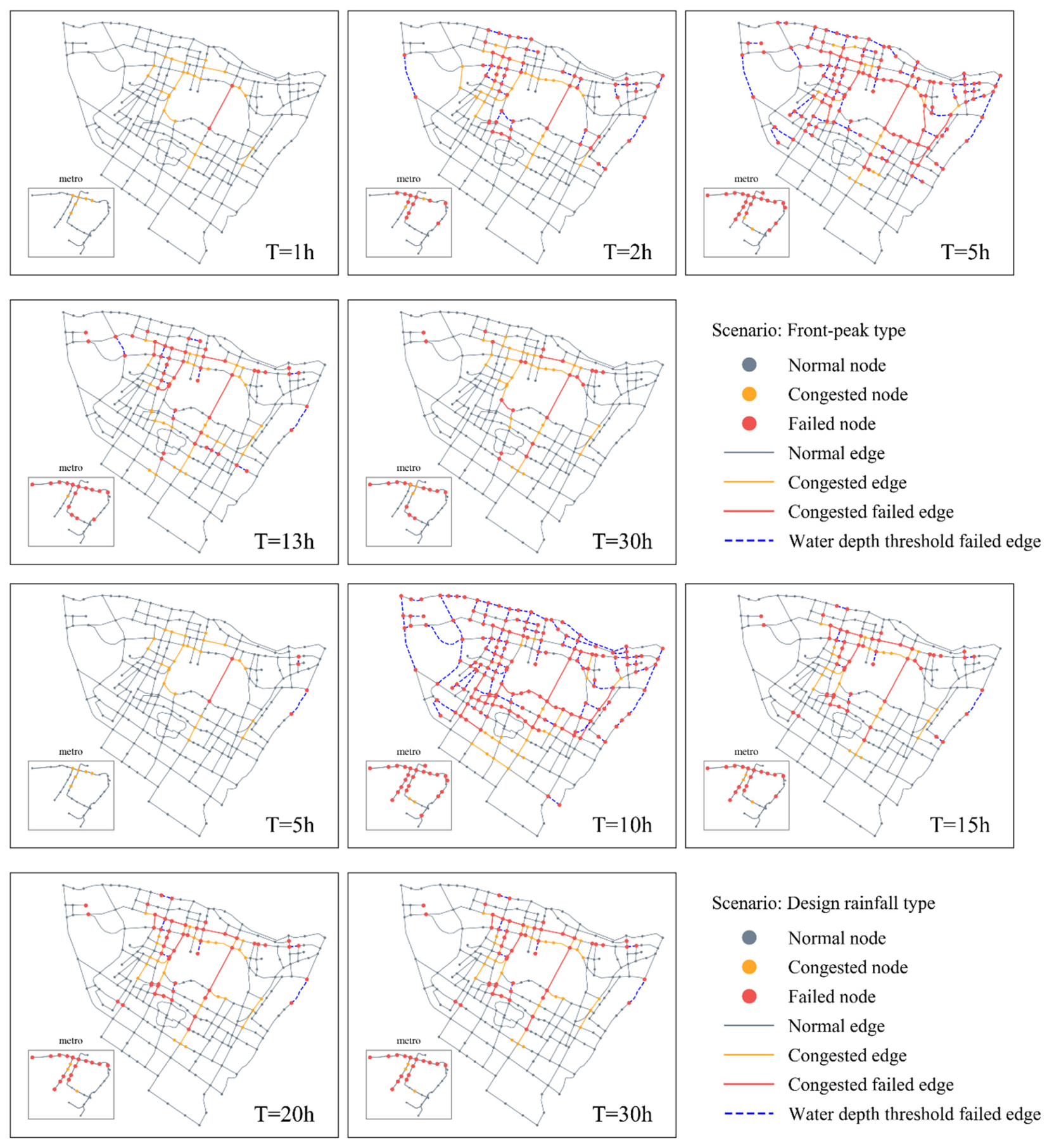
Seven rainfall-pattern scenarios with a 100-year return period were analyzed to examine the dynamic response of the transportation network during the pre-peak accumulation, peak expansion, and post-peak recovery stages. In all scenarios, failed and congested road segments initially appeared near the northern edge of the network, in the high-density road network area slightly north of the center, along the northeastern connecting corridors, and around rail-transfer nodes. These failures then expanded outward through backbone roads and key connecting edges. This spatial pattern suggests that rainstorm disturbances initially induce congestion at locally vulnerable nodes and bridging edges, which subsequently evolve into network failures that propagate through major transport corridors. Although most peripheral roads recovered relatively quickly after the rainfall peak, residual congestion and failures persisted in backbone corridors, connecting sections, and rail-transfer areas, indicating that transportation network recovery lagged behind rainfall recession. The Front-peak and Design rainfall types are illustrated in Figure 11 as representative examples.

Identifying the trigger points of cascading failures reveals that network risks do not propagate uniformly but are instead concentrated and amplified at a limited number of critical road sections and transfer stations. On the surface road layer, certain near-station sections and intersection nodes enter failure or high-congestion states first due to water accumulation. This initial disruption then causes sustained congestion on surrounding roads through load transfer, producing a pronounced diffusion and amplification effect. The main high-risk roads include Moshui Lake Bridge, Qintai Avenue, the Longyang Avenue intersection, Longxing East Street, and Longyanghu East Road. On the subway layer, the closure of key transfer stations simultaneously weakens connections between subway lines and transfer points, further intensifying traffic pressure in surrounding areas. The key trigger points on the subway network are Yulong Road, Hanyang Railway Station, Hanyang Passenger Station, and Wuliudun Station.

Further temporal analysis indicates that the cascading failure of the transportation network is triggered primarily by direct water-induced failure, while congestion mainly contributes to subsequent amplification. Here, “congestion expansion” refers to the increase in the number of congested edges, and “direct failure due to water depth exceeding the threshold” refers to the increase in the number of road edges that fail because water depth surpasses the threshold. The study compares the time difference between the onset of these two increases.

The results show that, in the seven primary scenarios, the number of failed edges due to water accumulation generally begins to rise earlier than or simultaneously with the number of congested edges. Considering only congested edges, the average time difference between the two is −2.86 h; when both congested edges and overload failure edges are considered, the average time difference is −1.14 h. The negative values indicate that the increase in water-induced failures occurs earlier than the increase in congestion-related edges.

These findings suggest that direct failure caused by water accumulation is usually the initial disturbance. In other words, although some degree of congestion already exists in the network at the initial moment, this initial congestion does not precede the network degradation process relative to failures caused by water accumulation. More commonly, certain roads fail first due to water accumulation, causing traffic flow to redistribute onto the remaining roads, which then triggers more extensive congestion expansion and localized overload failures. Thus, from a temporal perspective, water accumulation is the primary trigger of network failure, while congestion serves as the key mechanism that amplifies cascading degradation following the effects of water accumulation.

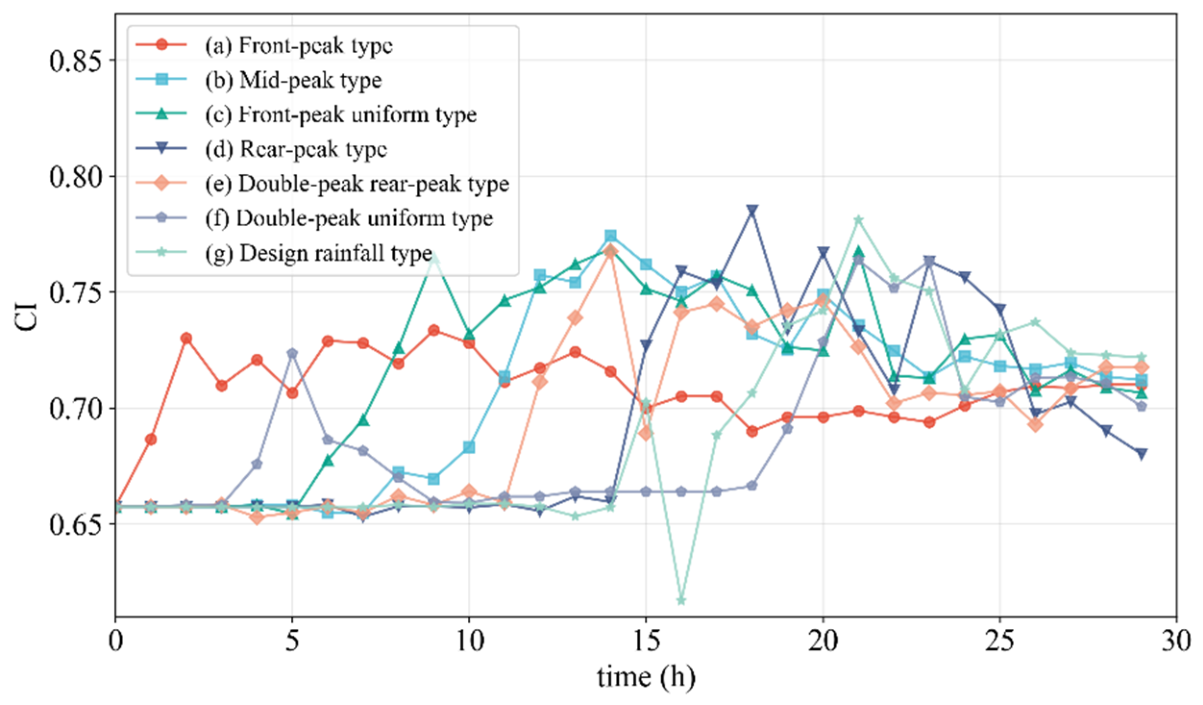
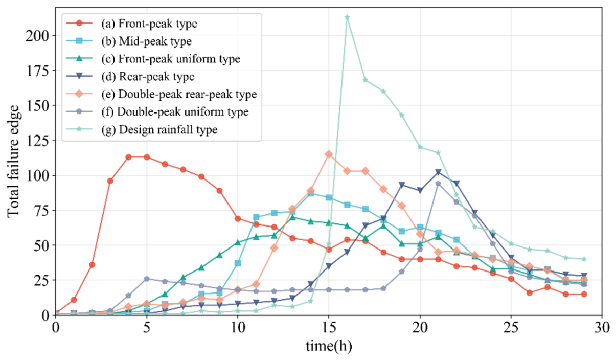
From the perspective of dominant factors, at the moment when the total number of failed edges reaches its peak, the average proportion of water depth failure edges is approximately 69.70%, with a weighted proportion of about 70.10%. These values are significantly higher than the 30.30% and 29.90% corresponding to congestion failure edges. This indicates that the large-scale failure of the traffic network is primarily driven by direct failure due to water accumulation. Phased analysis further reveals that during the pre-peak growth stage, the peak stage, and the post-peak attenuation stage, the proportion of water depth failure edges consistently exceeds that of congestion failure edges. This suggests that water accumulation has maintained a dominant role throughout the process, while congestion mainly acts as an amplifying mechanism that exacerbates local degradation and delays recovery. In conclusion, the failure of the traffic network is not solely determined by water accumulation or congestion alone but results from a coupled effect dominated by direct failure due to water accumulation and supplemented by the propagation effects of congestion. The temporal changes in the overall congestion index (CI) and the total number of failed sections under different scenarios are shown in Figure 12 and Figure 13. Although no extreme CI values were observed, the network still exhibited significant functional degradation, indicating that while overall connectivity did not completely collapse, local disorder and declines in service capacity continued to intensify.

The variation in CI and the number of failed edges further reveals that the cascading failure process differs systematically across rainfall patterns. During the peak stage, failure intensity was primarily controlled by the direct effect of extreme rainfall on road traffic capacity, whereas the post-peak stage more strongly reflected the persistent influence of congestion propagation following network load redistribution. These inter-scenario differences were closely associated with maximum rainfall intensity (P_max), rainfall concentration degree (PCT), peak magnitude (PUP), and asymmetry (ASY).

Among the seven scenarios, the Design rainfall type exhibited the highest P_max and produced the most severe ponding during the rainfall peak, resulting in the greatest number of failed edges. However, its CI peak remained comparatively limited, suggesting that extreme rainfall intensity primarily governs the upper bound of direct physical disruption rather than the full extent of congestion propagation. In contrast, the Front-peak type showed the earliest onset of failure, the fastest expansion, and the slowest dissipation of post-peak congestion. The Mid-peak and Rear-peak types sustained high-load operation and congestion propagation for longer durations, while the double-peak patterns demonstrate that cascading failure depends not only on the magnitude of a single peak but also on the temporal structure of the rainfall process. Overall, P_max determines the upper limit of failure intensity; PCT and PUP influence the rate and concentration of failure expansion; and ASY affects whether failure is more likely to intensify during the early or late stages.

Clear spatiotemporal contrasts were also observed among rainfall patterns. The Front-peak type was characterized by rapid early degradation, with failures concentrated along the northern edge, the north-central area, and the northeastern connecting corridors. The Mid-peak type was more likely to sustain a high-load state during the peak stage, whereas the Rear-peak and double-peak patterns exhibited more pronounced lag effects, with the network often shifting from local congestion to broader structural degradation in the later stages. Driven by its delayed rainfall centroid and extremely high peak, the Design rainfall type saw failure expand toward the main trunk corridors and central connecting areas. Even after rainfall weakened, network recovery remained delayed and residual congestion persisted. Overall, these findings suggest that highly concentrated and intense rainfall not only amplifies peak damage but also prolongs recovery pressure and lag effects within the transportation network.

4.2. Spatiotemporal Distribution Characteristics of Urban Waterlogging Risk

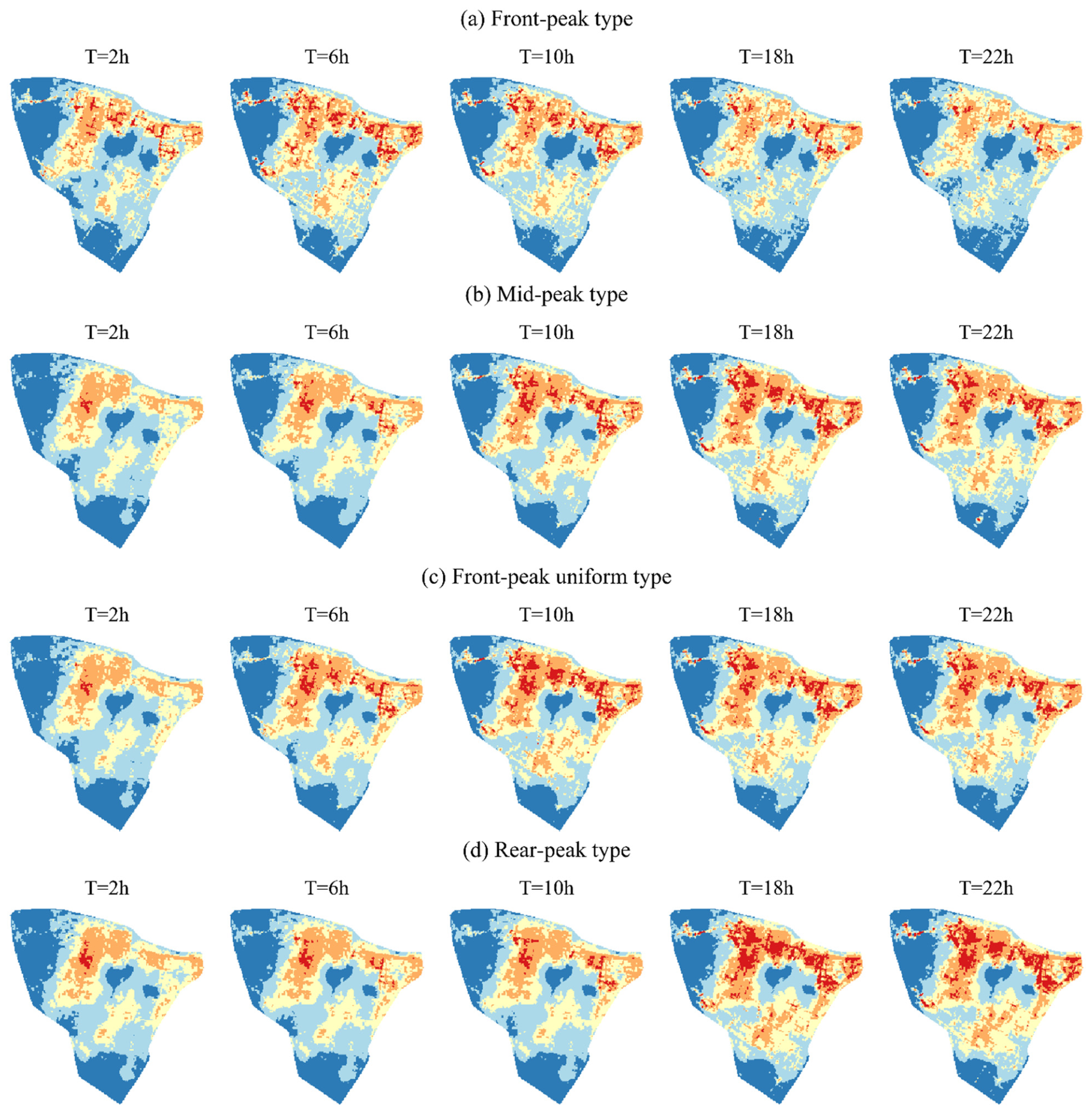
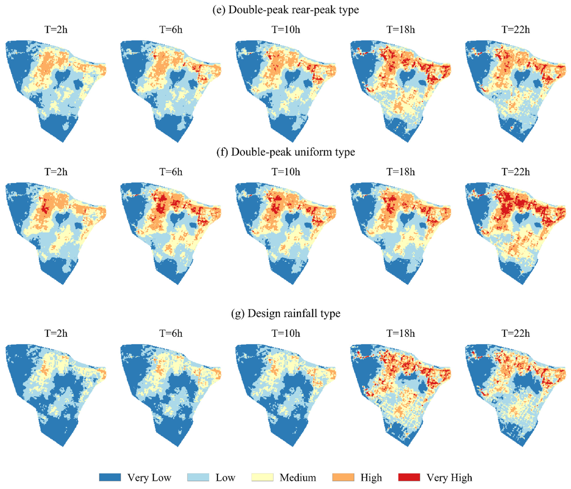
The spatiotemporal evolution of urban waterlogging risk under different scenarios was assessed according to the indicator weights determined above. Five time points corresponding to rainfall durations of 2, 6, 10, 18, and 22 h were selected for a unified comparison, as shown in Figure 14. Significant differences were observed in the temporal evolution of urban waterlogging risk among the different scenarios, and the location, extent, and duration of the maximum risk level varied substantially among the rainfall patterns.

From a spatial perspective, the high-risk and extremely high-risk areas under the Front-peak and Design rainfall types were relatively scattered and exhibited weak spatial continuity, reflecting concentrated rainfall peaks and a tendency for risk to emerge abruptly from multiple localized sources. In contrast, the extremely high-risk areas under the Mid-peak, Front-peak uniform, Rear-peak, and Double-peak uniform types were more spatially concentrated and expanded progressively outward from the center. Regarding the initial locations of extremely high risk, the Mid-peak, Rear-peak, and Double-peak uniform types all showed early emergence along Longyang Avenue, followed by gradual development toward the vicinity of Macanghu Road. However, under the Double-peak rear-peak type, extremely high risk first appeared near Macanghu Road. These differences suggest that the spatial sensitivity of the study area varies with rainfall patterns.

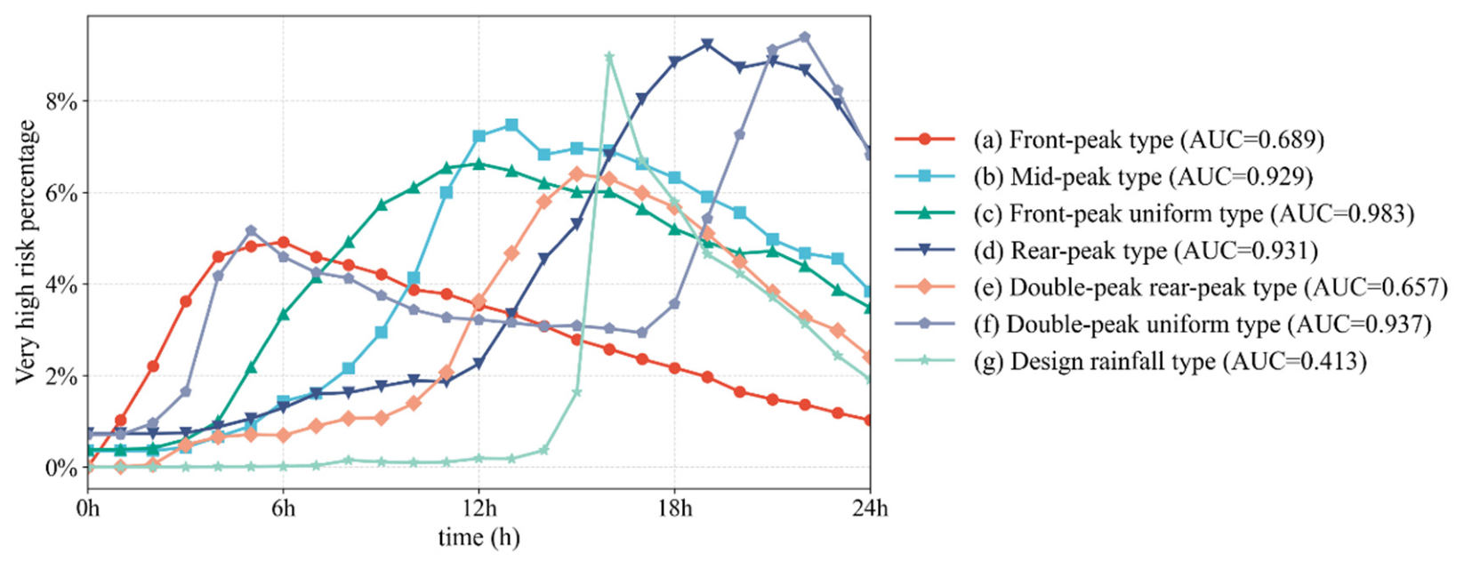
Further insight can be gained by examining the temporal variation in the proportion of extremely high-risk areas under different rainfall patterns, as shown in Figure 15. For the Front-peak type, the rainfall peak occurred at the 2nd hour, when the proportion of extremely high risk was 1.02%. This proportion then increased, reaching a peak of 4.91% at the 6th hour, before gradually declining to 1.48% by the 22nd hour, indicating a pattern of rapid early growth followed by relatively slow contraction. For the Mid-peak type, the rainfall peak appeared at the 11th hour; however, a small, extremely high-risk area had already emerged along Longyang Avenue in the early stage of rainfall, accounting for 0.36%. One hour before the rainfall peak, the proportion of high risk reached 17.19%, while the proportion of extremely high risk increased to 4.14%. By the 14th hour, the proportion of extremely high risk peaked at 7.47%, and the proportion of high risk reached 18.97%. This indicates that the peak of extremely high risk lagged behind the rainfall peak by 3 h. Although the proportion of extremely high risk decreased to 4.76% by the 22nd hour, it remained comparatively high. For the Front-peak uniform type, the proportion of extremely high risk was 0.39% at the 2nd hour, reached a peak of 6.62% at the 13th hour, and then decreased to 4.72% by the 22nd hour. Although the Front-peak uniform type and the Mid-peak type showed similar risk levels at the 2nd and 22nd hours, their evolutionary trajectories differed markedly. Their maximum hourly rainfall intensities were 23.86 mm and 35.91 mm, respectively, suggesting that the timing of the rainfall peak played an important role in shaping risk evolution. From the rainfall peak to the maximum proportion of extremely high risk, the Mid-peak type required only 3 h and exhibited a sharp rise in risk, whereas the Front-peak uniform type required 8 h and showed a slower but more sustained increase. Both patterns exhibited continued late-stage risk accumulation, indicating a stronger tendency toward the persistent expansion of medium- and high-risk areas.

For the Rear-peak type, the rainfall peak occurred at the 17th hour, while the extremely high risk reached its maximum value of 9.22% at the 20th hour. Except for the Design rainfall type, the Double-peak rear-peak type exhibited the lowest proportion of extremely high risk in the early stage. Its main rainfall peak occurred at the 14th hour, and the maximum proportion of extremely high risk appeared at the 16th hour at 6.40%, after which the risk declined. In comparison, the Double-peak uniform type showed a pronounced two-stage increase in extremely high risk, reaching 5.16% and 9.29% at the 6th and 23rd hours, respectively. After increasing following the first rainfall peak, the risk decreased to 2.93% before rising again, producing the highest proportion of extremely high risk among the seven rainfall patterns. Under the Design rainfall type, the proportion of extremely high risk remained below 0.4% in the early stage but surged to a maximum of 8.97% only 2 h after the rainfall peak, before declining to 0.37% at the 22nd hour. This final value was markedly lower than those under the Mid-peak type, Front-peak uniform type, Rear-peak type, and Double-peak rear-peak type. The subsequent decline was also substantially faster, indicating that the Design rainfall type is characterized by pronounced suddenness and concentrated risk release.

A comparison of peak values further highlights the differences among rainfall patterns. Regarding the maximum proportion of extremely high risk, the Double-peak uniform type ranked highest, followed by the Rear-peak type and the Design rainfall type. Next in sequence were the Double-peak rear-peak type, the Mid-peak type, the Front-peak uniform type, and the Front-peak type. Although the Design rainfall type produced a relatively high peak proportion of extremely high risk, its duration of high risk was comparatively short. In contrast, the Double-peak uniform type and the Rear-peak type were associated with a higher overall risk level. To further evaluate the persistence of extremely high risk, the area under the curve representing the proportion of extremely high risk over the statistical duration of 0–30 h was calculated. The results indicate that the Front-peak uniform type exhibited the greatest persistence of extremely high risk, despite its peak ranking only sixth. Although the Double-peak uniform type had the highest peak proportion of extremely high risk, it ranked second in persistent risk, followed by the Rear-peak type and the Mid-peak type, both with values greater than 0.9. The Front-peak type and the Double-peak rear-peak type ranked next, whereas the Design rainfall type showed the lowest persistent risk, at only 0.413. Taken together, the peak proportion of extremely high risk reflects the maximum danger associated with a given rainfall pattern, whereas persistence intensity better captures the duration of hazardous conditions throughout the rainfall event.

4.3. Dynamic Variation Process of Urban Waterlogging Risk

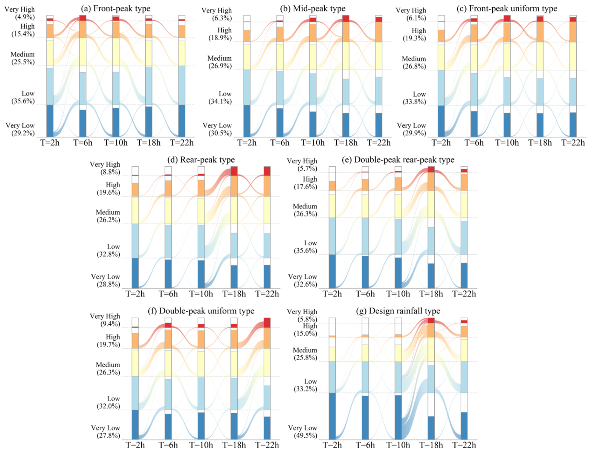
To further characterize the dynamic transformation of risk levels under different rainfall-pattern scenarios, the amplitude and direction of risk evolution were analyzed based on the proportion of each risk level during each period and its alluvial-flow direction, as shown in Figure 16. Different colors represent the proportions of various risk levels at different times; the banded strips indicate the direction of risk-level transitions, and the strip width corresponds to the proportion of risk that changed during the respective period. The risk-level proportions labeled on the vertical axis denote the maximum values among the five statistical time points. For comparability, the same time points were used across all scenarios. Overall, risk accumulated persistently under all rainfall-pattern scenarios and exhibited staged jumps in risk-level transitions, although the timing and intensity of these transitions varied markedly among rainfall patterns.

From the perspective of transformation pathways, risk evolution in most scenarios was dominated not by abrupt jumps between extreme levels but by gradual escalation. In the Front-peak type, the main changes during 2–6 h were increases of 7.14% in low risk and 4.77% in medium risk, indicating a typical early diffusion-type escalation. In the Mid-peak type, the primary increases during 10–18 h were 6.25% in low risk, 3.51% in medium risk, and 2.50% in high risk, suggesting that medium- and high-risk areas deepened further in the later stage of rainfall. The Front-peak uniform type showed both a pronounced early increase during 2–6 h, with 7.17% of low risk and 6.50% of medium risk upgraded, and a clear persistence of escalation during 6–10 h and 10–18 h, reflecting a relatively long period of risk accumulation. By comparison, the Rear-peak type and the Double-peak rear-peak type displayed more abrupt transformations, with the proportions of risk increase during 10–18 h reaching 32.23% and 29.35%, respectively. The most distinctive feature of the Double-peak uniform type was lagged intensification: during 18–22 h, the proportion of risk increase remained as high as 26.91%, and the proportion of high risk rose further to 29.06% at the 22nd hour, the highest among all scenarios. This pattern indicates a sustained amplification effect in the later stage.

Overall, the Front-peak type was characterized by early-stage expansion followed by a relatively rapid recovery. The Mid-peak type, Front-peak uniform type, Rear-peak type, and Double-peak rear-peak type all exhibited steady increases in risk transition, whereas the Double-peak rear-peak type maintained continued growth in the later stage. In contrast, the Design rainfall type showed a concentrated increase in risk level with a pronounced, jump-like escalation. Taken together, these patterns suggest that differences in rainfall patterns affect not only the final extent of high-risk areas but also the timing and duration through which risk propagates from lower to higher levels. From the perspective of risk warning and control, attention should therefore be directed not only to the final proportion of high-risk areas but also to the key transition periods under each scenario, so that targeted interventions can be implemented before risk is rapidly amplified.

4.4. Advantages of the Dynamic Risk Assessment Framework

To demonstrate the advantage of incorporating dynamic indicators while maintaining the established weights, we conducted a statistical association analysis between three dynamic road network indicators—Dynamic Load Ratio (DLR), Accessibility of Emergency Response (AL), and Undersized Drainage Ratio (UDR)—and both the comprehensive risk values and their corresponding dimensional scores. Specifically, using the existing risk assessment results, we extracted the values of the three dynamic indicators for each grid unit at each time step and calculated their respective risk contribution terms according to the established standardization and positive/negative direction processing rules. Based on this, we computed the Pearson and Spearman correlation coefficients between these indicators and both the comprehensive risk values and the scores of their respective dimensions.

The results show that DLR exhibits a strong positive correlation with both the comprehensive risk and the exposure dimension scores. The overall Pearson correlation coefficient between DLR and comprehensive risk is 0.743, while that between DLR and exposure dimension scores is 0.707. Across different time periods, the correlation with comprehensive risk ranges from 0.335 to 0.867. This indicates that DLR can effectively characterize the amplifying effect of changes in road carrying pressure on risk exposure during rainfall events. UDR shows a relatively weak direct correlation with comprehensive risk, with an overall Pearson correlation coefficient of −0.166; however, its correlation with the vulnerability/response capacity dimension scores is as high as 0.979, ranging from 0.392 to 0.999 across different periods. This suggests that UDR primarily compensates for the inadequacy of static assessments in depicting dynamic storage and regulation capacity by modifying the drainage carrying capacity. AL exhibits an overall Pearson correlation coefficient of −0.269 with comprehensive risk and 0.235 with the capacity dimension scores, indicating a generally weak correlation. Nevertheless, during the 16 h–18 h period under the design rainfall scenario, its correlation with the capacity dimension reaches 0.813 to 0.903, implying that its impact on risk is distinctly phase-specific and more suitable for characterizing emergency support disparities during critical time windows.

Furthermore, regarding the average weighted contribution shares of the three dynamic indicators to the comprehensive risk, UDR, DLR, and AL account for approximately 17.20%, 8.07%, and 0.55%, respectively. Overall, these three dynamic indicators are not merely simple additions to the comprehensive weighting system; rather, they enhance the capability of traditional static assessments to characterize the temporal evolution of risk from three perspectives: traffic exposure, drainage carrying capacity, and emergency response.

5. Discussion

Compared to assessments based solely on ponding depth or static exposure distribution, this study demonstrates that dynamic risk assessment more accurately reflects the degradation of urban functionality during a waterlogging event, rather than simply indicating the locations of inundation. Furthermore, in the hydrodynamic simulation, underground-space storage capacity was incorporated to better represent the redistribution of stormwater between the surface and subsurface domains. This distinction is especially important in sustainability-oriented urban management. Risk arises not only from physical exposure but also from disruptions to mobility, accessibility, and service continuity. Our findings are consistent with studies highlighting the temporal co-evolution of hazard, exposure, and vulnerability during flood events [5,7]. They further develop this perspective by explicitly incorporating the coupled response of surface and underground transportation systems into the risk assessment process.

The transportation-related findings also align with previous evidence indicating that flood impacts on urban mobility are influenced by both direct inundation and network-mediated disruptions. Studies of urban transport and subway systems have demonstrated that roads, stations, and transfer facilities can act as critical failure points during flood conditions [10,11,13,14]. Similarly, our results indicate that traffic-capacity degradation, path redistribution, and cascading failures are not merely isolated technical effects but are key mechanisms through which localized waterlogging evolves into broader spatial inequalities in urban accessibility. Direct inundation is the primary trigger of large-scale network degradation, whereas congestion mainly acts as a secondary amplification mechanism by redistributing traffic loads after part of the road network has already been disrupted by flooding. This interpretation is also consistent with recent findings that congestion diffusion can substantially intensify, rather than independently initiate, the degradation of road network performance under rainfall-induced flooding [20].

Dynamic accessibility is critical for emergency response and urban resilience. Previous studies have reported that emergency service accessibility is highly sensitive to changes in road network functionality during flood events [12,25,26]. Our results further demonstrate that the timing and duration of accessibility loss vary significantly across different rainfall patterns, indicating that relying solely on static risk maps may underestimate the urgency of timely interventions. For sustainable urban governance, this implies that drainage scheduling, traffic diversion, and emergency resource allocation should be coordinated not only according to the anticipated extent of inundation but also considering the evolving functional state of the interconnected transportation infrastructure.

The comparison of rainfall pattern scenarios also has broader planning implications. Rather than viewing urban waterlogging simply as a result of total rainfall, our findings demonstrate that the temporal pattern of rainfall significantly affects the timing of system disturbances, the delay in high-risk accumulation, and the persistence of disruptions following peak rainfall. This suggests that sustainable adaptation strategies should transition from static zoning to time-sensitive, infrastructure-conscious risk management. In practice, front-peak events require earlier traffic interventions, while rear-peak and double-peak events demand greater focus on delayed recovery, sustained drainage operations, and extended emergency preparedness.

Nevertheless, several limitations should be acknowledged. First, traffic demand and mobility behavior have yet to be represented using trajectory data with higher temporal resolution. The current research focuses on the differences in traffic network failures under various rainfall patterns, rather than a reconstruction of real events. The analytical conclusions of this study help identify the vulnerability structure of the traffic network under rainfall conditions. Second, the inundation of underground spaces is modeled using a generalized storage-tank method, which is appropriate for regional-scale assessments but less effective at capturing fine-scale, microscopic inflow processes. Future research could enhance this framework by incorporating higher-resolution mobility data, refining the representation of underground spaces, and evaluating how alternative intervention strategies affect dynamic risk trajectories under different rainfall patterns.

6. Conclusions

This study developed a dynamic urban waterlogging risk assessment framework by integrating hydrodynamic simulation, a coupled surface–underground transportation system, and the H-E-V-C framework under multiple rainfall-pattern scenarios in Hanyang District, Wuhan. The main conclusions are as follows.

(1) Direct inundation is the main trigger of large-scale transportation-network degradation, while congestion and local overload further amplify cascading failures. Based on the results of different rainfall patterns, the roads with high structural risks include Moshui Lake Bridge, Qintai Avenue, the Longyang Avenue intersection, Longxing East Street, and Longyanghu East Road. The most vulnerable subway stations include Yulong Road, Hanyang Railway Station, Hanyang Passenger Station, and Wuliudun.

(2) Rainfall-pattern structure affects not only the maximum disruption of the transportation network but also the timing, duration, and spatial expansion of high-risk areas. Front-peak events tend to cause earlier deterioration, whereas rear-peak and double-peak events more often lead to delayed or sustained risk amplification.

(3) By incorporating dynamic indicators such as road-load distribution, emergency response time, and non-overloaded pipe-network density, the framework better identifies transfer nodes, backbone corridors, and areas with reduced emergency accessibility, thereby improving the spatiotemporal interpretation of urban waterlogging risk.

(4) Traffic control, drainage scheduling, and emergency resource deployment should be aligned with rainfall-pattern-specific transition periods and persistently high-risk areas, rather than relying only on static inundation maps.

References

1. UNDRR. Sendai Framework Terminology on Disaster Risk Reduction; United Nations Office for Disaster Risk Reduction: Geneva, Switzerland, 2017. [Google Scholar]
2. IPCC. The Concept of Risk in the IPCC Sixth Assessment Report: A summary of Cross Working Group Discussions; Intergovernmental Panel on Climate Change: Geneva, Switzerland, 2021. [Google Scholar]
3. Zhang, H.; Li, C.; Cheng, J.; Wu, Z.; Wu, Y. A review of urban flood risk assessment based on the framework of hazard-exposure-vulnerability. Prog. Geogr. 2019, 38, 175–190. [Google Scholar] [CrossRef] [Scilit]
4. Huang, G.; Luo, H.; Lu, X.; Yang, C.; Wang, Z.; Huang, T.; Ma, J. Study on risk analysis and zoning method of urban flood disaster. Water Resour. Prot. 2020, 36, 1–6+17. [Google Scholar] [CrossRef] [Scilit]
5. Lazzarin, T.; Viero, D.P.; Molinari, D.; Ballio, F.; Defina, A. A new framework for flood damage assessment considering the within-event time evolution of hazard, exposure, and vulnerability. J. Hydrol. 2022, 615, 128687. [Google Scholar] [CrossRef] [Scilit]
6. Han, F.; Yu, J.; Zhou, G.; Li, S.; Sun, T. Projected urban flood risk assessment under climate change and urbanization based on an optimized multi-scale geographically weighted regression. Sustain. Cities Soc. 2024, 112, 105642. [Google Scholar] [CrossRef] [Scilit]
7. He, W.J.; Zeng, J.; Zhang, J.H.; Namaiti, A.; Shi, W.H.; Song, Y.Z.; Tian, J. Dynamic urban flood risk assessment based on human activity patterns: An IFAHP-EWM-TOPSIS approach. Sustain. Cities Soc. 2025, 133, 105705. [Google Scholar] [CrossRef] [Scilit]
8. Xiang, H.T.; Lyu, H.M. Assessment of vulnerability to waterlogging in subway stations using EWM-TOPSIS. Discov. Civ. Eng. 2023, 3, 17. [Google Scholar] [CrossRef] [Scilit]
9. Borowska-Stefańska, M.; Bartnik, A.; Dulebenets, M.A.; Kowalski, M.; Sahebgharani, A.; Tomalski, P.; Wiśniewski, S. Changes in the equilibrium of the urban transport system of a large city following an urban flood. Reliab. Eng. Syst. Saf. 2025, 253, 110473. [Google Scholar] [CrossRef] [Scilit]
10. Wu, W.; Zhu, Z.; Zheng, X.; Liu, S.; Zhang, D.; Peng, D.; Pang, B. A flood risk assessment framework for urban subway systems: A case study in Beijing, China. Sustain. Cities Soc. 2025, 131, 106681. [Google Scholar] [CrossRef] [Scilit]
11. Zhang, K.H.; Mei, C.; Liu, J.H.; Wang, J.; Song, T.X.; Shi, H.Y.; Dong, L.R.; Li, Y.L.; Zhang, A.Q. Impact assessment of urban waterlogging on roads trafficability and emergency sites accessibility under extreme rainfall events based on numerical modeling. Int. J. Disaster Risk Reduct. 2025, 119, 105285. [Google Scholar] [CrossRef] [Scilit]
12. Xu, F.; Fang, D.L.; Chen, B.; Wang, H. Resilience assessment of subway system to waterlogging disaster. Sustain. Cities Soc. 2024, 113, 105710. [Google Scholar] [CrossRef] [Scilit]
13. Xu, P.C.; Lu, Q.C.; Feng, T.; Li, J.; Li, G.; Xu, X. Resilience analysis of metro stations integrating infrastructures and passengers. Reliab. Eng. Syst. Saf. 2024, 252, 110467. [Google Scholar] [CrossRef] [Scilit]
14. Erdem, U.; Sharifi, A.; Ökmen, Z. Neighborhood-scale assessment of urban flood impacts on transportation network resilience: A case study of Mavişehir, İzmir. Int. J. Disaster Risk Reduct. 2026, 132, 105970. [Google Scholar] [CrossRef] [Scilit]
15. Qi, W.; Ma, C.; Xu, H.; Zhao, K. Urban flood response analysis for designed rainstorms with different characteristics based on a tracer-aided modeling simulation. J. Clean. Prod. 2022, 355, 131797. [Google Scholar] [CrossRef] [Scilit]
16. Zhang, M.; Xu, M.; Wang, Z.; Lai, C. Assessment of the vulnerability of road networks to urban waterlogging based on a coupled hydrodynamic model. J. Hydrol. 2021, 603, 127105. [Google Scholar] [CrossRef] [Scilit]
17. Guo, Y.; Wang, L.; Chen, N.; Jin, J. Simulation of the flood process in urban surface- underground space under extreme rainfall. Adv. Water Sci. 2023, 34, 209–217. [Google Scholar]
18. Song, T.; Liu, J.; Mei, C.; Wang, J.; Zhang, K.; Shi, H. Research on the Influence of Underground Space on Urban Waterlogging in Extreme Rainfall. J. Basic Sci. Eng. 2024, 32, 349–364. [Google Scholar]
19. Yuan, X.M.; Wu, M.R.; Tian, F.C.; Wang, X.J.; Wang, R.K. Identification of influencing factors and risk assessment of underground space flooding in the mountain city. Int. J. Disaster Risk Reduct. 2024, 113, 104807. [Google Scholar] [CrossRef] [Scilit]
20. Chen, Z.; Zheng, C.; Xu, M.; Wu, Z.; Zheng, S.; Ma, G. Quantitative assessment of congestion diffusion and cascading effect under rainfall-flood disasters: A case study of Nanjing, China. Int. J. Disaster Risk Reduct. 2024, 114, 104915. [Google Scholar] [CrossRef] [Scilit]
21. Huang, G.; Li, M. Research progress on impact assessment of urban waterlogging on road traffic based on micro traffic simulation. Water Resour. Prot. 2023, 39, 69–78. [Google Scholar]
22. Du, L.; Yang, X. A Study on the Impact of Road Flooding on Traffic and the Resulting Losses. In Proceedings of the Technological Innovation and Green Transportation—The 11th National Academic Conference on Urban Road Transportation, Dalian, China, 1 October 2011; pp. 389–393. [Google Scholar]
23. Shah, S.M.H.; Mustaffa, Z.; Martinez-Gomariz, E.; Kim, D.K.; Yusof, K.W. Criterion of vehicle instability in floodwaters: Past, present and future. Int. J. River Basin Manag. 2019, 19, 1–23. [Google Scholar] [CrossRef] [Scilit]
24. He, K.; Pregnolato, M.; Carhart, N.; Neal, J.; De Risi, R. Functionality assessment of road network combining flood roadworthiness and graph topology. Transp. Res. Part D-Transp. Environ. 2024, 135, 104354. [Google Scholar] [CrossRef] [Scilit]
25. Zang, Y.; Huang, J.; Wang, H. Dynamic impact assessment of urban floods on the compound spatial network of buildings-roads-emergency service facilities. Sci. Total Environ. 2024, 926, 172007. [Google Scholar] [CrossRef] [Scilit] [PubMed]
26. Mitropoulos, L.; Karolemeas, C.; Tsigdinos, S. Road network accessibility assessment during flood events by using infrastructure facility-based indices. Int. J. Disaster Risk Reduct. 2025, 122, 105475. [Google Scholar] [CrossRef] [Scilit]
Figure 1. Study Area Overview and Model Boundaries.
Sustainability 18 06558 g001
Figure 2. Rainfall Pattern Recognition Results and Rainfall Distribution Ratios.
Sustainability 18 06558 g002
Figure 3. The 24-Hour Design Rainfall Curve.
Sustainability 18 06558 g003
Figure 4. Simplified diagram of an underground space.
Sustainability 18 06558 g004
Figure 5. A framework for assessing urban flooding risks by coupling the dynamic responses of the transport network.
Sustainability 18 06558 g005
Figure 6. Evaluation indicator weights.
Sustainability 18 06558 g006
Figure 7. Comparison of simulated water levels during the rainfall event on 30 June 2016.
Sustainability 18 06558 g007
Figure 8. Simulation of water accumulation during the rainfall on 7 July 2013 (The red area indicates the areas prone to water accumulation).
Sustainability 18 06558 g008
Figure 9. Spatial distribution of static indicators.
Sustainability 18 06558 g009
Figure 10. Spatial distribution of dynamic indicators (global normalization, taking the design rainfall at different times as an example).
Sustainability 18 06558 g010aSustainability 18 06558 g010b
Figure 11. Dynamic response process of the surface–underground transportation network under different scenarios.
Sustainability 18 06558 g011
Figure 12. Overall congestion index CI changes in different scenarios.
Sustainability 18 06558 g012
Figure 13. Total number of failure edges in different scenarios.
Sustainability 18 06558 g013
Figure 14. Dynamic changes in flood risk under different rainfall scenarios.
Sustainability 18 06558 g014aSustainability 18 06558 g014b
Figure 15. The process of changes in the proportion of extremely high-risk levels in different scenarios.
Sustainability 18 06558 g015
Figure 16. The process of dynamic changes in areas at risk of flooding over time at different risk levels.
Sustainability 18 06558 g016