Computational Flow Analysis of a Passive Control Windmill Sail Rotor with Field Measurement Verification

Abstract

This study presents a computational and experimental aerodynamic characterisation of a full-scale 5.5 m diameter, six-sail horizontal-axis windmill of the traditional Cretan Lasithi type, equipped with flexible woven polyester sails that act as a passive load-control mechanism. Seventeen operating points spanning wind speeds of 2.3–18.3 m/s were simulated in OpenFOAM using a transient sliding-mesh Arbitrary Mesh Interface formulation with the k–ω SST turbulence closure on a 2.3 million cell grid, selected on the basis of a four-level grid convergence study. CFD simulations identify three distinct aerodynamic regimes: a drag-dominated high-TSR regime (λ > 2.1), a mixed lift–drag working range with peak loading near λ ≈ 1.4–1.5, and a deep-stall regime in which boundary-layer separation propagates from root to tip as λ falls below 1.0. Field measurements conducted at the Energy Systems Synthesis Lab of the Hellenic Mediterranean University in compliance with IEC 61400-12-1:2005(E) confirm that rotor speed stabilises passively at 55–58 RPM above 13 m/s without any active control mechanism; CFD predictions agree with measured power output within 8–12% across the 2–13 m/s attached-flow envelope. The combined evidence indicates that passive overspeed self-regulation is driven by aeroelastic sail deformation, reducing effective disc solidity at high wind speeds, a mechanism that rigid-geometry CFD correctly identifies in trend but cannot quantify in magnitude. The primary limitation of the present work is the rigid-sail assumption of the CFD model, which requires a two-way coupled fluid–structure interaction extension as a future step.

1. Introduction

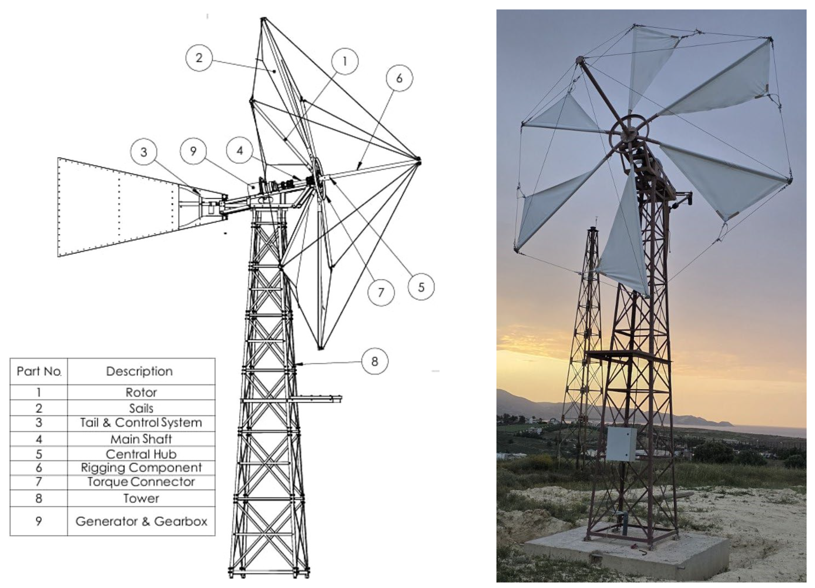
Nestled in eastern Crete, the Lasithi Plateau is a high-altitude plain of roughly 11 km by 6 km, situated approximately 840 m above sea level and encircled by mountain peaks. A defining feature of its 20th-century agricultural heritage was the proliferation of wind-pumps—locally crafted horizontal-axis windmills—that harnessed the region’s Aeolian resource to draw groundwater for irrigation. At their peak, these white-sailed structures numbered up to 10,000–13,000, forming a remarkable distributed wind system [1,2,3,4,5,6]. Initially constructed in wood around 1890, the machines later evolved through the introduction of metal towers and self-orienting mechanisms [1,2,3,4,5,6]. The traditional rotor included four to twelve triangular canvas sails fixed to a wooden frame. As it turned out, practical experience and ethnographic documentation showed that six- to eight-sail configurations became common practice, with higher solidity rotors favoured for heavier workloads or low-wind locations [3,6,7,8,9]. The six-sail design (Figure 1) examined in the present work balances aerodynamic efficiency with the operational and maintenance expectations of the Lasithi community and represents a direct continuation of a prior study of the same prototype, focused on aerodynamic and structural behaviour, before the field campaign measurements [10].

Computational fluid dynamics has become an indispensable tool in wind energy research, offering detailed insight into flow structures, torque generation, and the influence of operating conditions without the cost and logistical burden of exhaustive experimental campaigns [11,12]. Horizontal-axis wind turbines, from large utility-scale machines to small heritage-inspired rotors, depend on accurate CFD predictions for design optimisation, performance characterisation, and reliability assessment. OpenFOAM provides an open, well-validated environment for such studies [13,14], and its sliding-mesh Arbitrary Mesh Interface formulation is particularly well suited to the transient, rotating-domain problems that arise in rotor aerodynamics. The application of CFD to traditional and multi-bladed windmills has grown steadily but remains incomplete in several respects. Early experimental studies characterised multi-bladed cambered rotors in wind-tunnel environments, examining how solidity, Reynolds number, and blockage affect torque and power output across 3-, 6-, 12-, and 24-blade configurations [15]. Complementary helical-vortex and blade-element models were subsequently validated against those measured performance curves, improving predictive capability for high-solidity rotors [16]. Engineering-oriented work extended these findings to full wind-pump design workflows for specific regional wind regimes [17] and to experimental assessment of windmill-driven desalination systems at low wind speeds [18]. The most directly relevant prior computational study applied CFD-based aerodynamic analysis and finite-element structural modelling to reconstruct and evaluate the functional characteristics of historic Spanish windmills [12]. Also, graphical and geovisual analyses of the La Mancha windmills have provided momentum-based performance estimates and structural certification [19]. A broader historiographical thread traces the architectural and mechanical co-evolution of windmill forms across centuries [8,20] and documents Mediterranean examples through three-dimensional modelling and mechanical-parameter extraction [21]. Contemporary applications demonstrate that windmill-inspired geometries can support low-power energy harvesting [22], and earlier work introduced programmable windmill simulators for hardware-in-the-loop testing [23]. The reconversion of traditional Mallorcan water-extraction windmills into small-scale electrical generators has further demonstrated the technical feasibility of adapting heritage machines for modern energy use [24].

Despite the extensive literature covering traditional windmill simulations, several important gaps remain. (i) No systematic grid-convergence study has been reported for the Cretan sail-rotor class, leaving mesh-independent solutions undefined. (ii) No direct turbulence-model comparison has been conducted for this geometry, and the failure modes of the standard k–ε closure under post-design-point stall conditions have not been quantified. (iii) Critically, no prior study has combined a parametric CFD sweep with a full-scale field measurement campaign conducted under a recognised performance standard for this rotor class, meaning that the passive overspeed self-regulation mechanism and the aeroelastic load-shedding behaviour of the woven polyester sails have not been validated against real atmospheric data.

This study addresses these gaps through a combined computational and experimental characterisation of a full-scale six-sail Cretan windmill of the Lasithi type. The novelties of the current study are as follows. A combined computational and experimental characterisation of a full-scale Cretan sail-rotor windmill of the Lasithi type is presented, integrating a 17-case parametric transient CFD sweep—employing a sliding-mesh Arbitrary Mesh Interface (AMI) formulation with the k–ω SST turbulence model in OpenFOAM, with a dedicated field measurement campaign conducted under the IEC 61400-12-1:2005(E) framework. Unlike prior studies that addressed either the aerodynamic modelling or the historical documentation of traditional sail-rotor windmills separately, this work provides the first systematic four-level grid convergence study for this rotor class, identifying mesh-independent solutions at 2.3 million cells for the attached-flow operating range, and a direct turbulence model comparison demonstrating the failure of k–ε to capture blade-surface separation at post-design-point tip speed ratios. The application of the IEC method of bins directly to 1 s measurement data, without minute-level averaging, preserves the full turbulent content of the wind record and enables the first quantitative characterisation of the power coefficient and tip speed ratio behaviour of this rotor class under real atmospheric conditions. A further novelty is the experimental identification of the passive overspeed self-regulation mechanism inherent in flexible woven polyester sails, which produces a stable rotational speed range of 55 to 58 RPM above 10 m/s without any active pitch or furling system. A reversal in rotor speed above 16 m/s, coinciding with a surface pressure and wake topology transition, is independently verified by the CFD results, providing quantitative motivation for the planned future extension of fluid–structure interaction.

2. Theoretical Background

2.1. Principal Aerodynamic Parameters

The aerodynamic performance of a windmill is governed by the interaction of rotating sails with the oncoming wind stream. The tip speed ratio (TSR), defined as the ratio of blade tip speed to free-stream wind speed, is a key nondimensional parameter:

$$\begin{array}{c}\lambda =\left(\omega R\right)/U_{\mathrm{\infty }},\end{array}$$

(1)

where ω is the angular velocity (rad/s), R is the rotor radius, and $U_{\mathrm{\infty }}$ is the free-stream wind speed. Torque (Q) and power (P) are related through the equation:

$$\begin{array}{c}P=Q\omega .\end{array}$$

(2)

The power coefficient (C_p) and torque coefficient (C_q) are defined to normalise the windmill performance as:

$$\begin{array}{c}{C}_p=P/\left(0.5\rho A{U}_{\mathrm{\infty }}^3\right),\end{array}$$

(3)

$$\begin{array}{c}{C}_q=Q/\left(0.5\rho AR{U}_{\mathrm{\infty }}^2\right),\end{array}$$

(4)

where ρ is the air density, and A is the rotor swept area.

The pressure coefficient is determined by:

$$\begin{array}{c}{C}_{pres}=\left(p-p_{\mathrm{\infty }}\right)/\left(0.5\rho U_{\mathrm{\infty }}^2\right),\end{array}$$

(5)

And it is used to interpret blade loading distributions and identify flow separation in the CFD results. Accurate CFD modelling of these coefficients requires the correct resolution of boundary layers, wake interactions and the overall flow geometry distribution [25].

2.2. CFD Modelling Approach

The simulations solve the incompressible Reynolds-Averaged Navier–Stokes (RANS) equations in OpenFOAM [13,14]. Two turbulence closures are compared: the standard k–ε model and the k–ω SST model of Menter [26]. The k–ω SST formulation is adopted as the primary closure for the parametric sweep because it blends a k–ω treatment in the near-wall region, thus correctly capturing adverse pressure gradient effects and incipient separation on the curved sail surfaces, with a k–ε treatment in the free stream, which is less sensitive to inlet turbulence boundary conditions. The explicit eddy-viscosity limiter in the SST model prevents the unphysical overprediction of turbulent shear stress that causes the standard k–ε closure to suppress boundary-layer separation in rotating and adverse pressure gradient flows [26,27]. This deficiency is particularly pronounced in rotating flows, where the additional strain introduced by Coriolis and centrifugal acceleration amplifies the production-to-dissipation imbalance. For multi-bladed low-TSR rotors of the type investigated here, Sørensen et al. [28] and Tachos et al. [29] demonstrated that k–ε overpredicts shaft torque by 40–100% in the post-stall regime while k–ω SST reproduces measured performance within 10–20%, attributing the k–ε overestimation to the suppression of the leading-edge recirculation bubble that governs stall onset on low-chord-Reynolds-number sail surfaces. This discrepancy is demonstrated directly in Section 5. These characteristic assets of the k–ω SST model make it the established standard for separated aerodynamic flows in the wind energy community, as confirmed by the comprehensive reviews of Vermeer et al. [30] and Porté-Agel et al. [25].

Model constants and boundary condition settings follow the standard values given in Menter [26] and Greenshields & Weller [31]. Inlet turbulence is specified according to the measurement site conditions described in Section 4.

The CFD workflow employs two complementary rotation strategies. In the steady-state initialisation phase, the Multiple Reference Frame (MRF) approach adds pseudo-force source terms to the momentum equations within the rotating zone, producing a well-converged initial flow field at a low cost. In the subsequent transient phase, the mesh within the rotating zone physically rotates at each time step via a sliding-mesh Arbitrary Mesh Interface (AMI), which interpolates field values across non-conformal face pairs using an area-weighted overlap algorithm. Full details of the solver settings, time-stepping, and convergence criteria are given in Section 3.

3. Computational Methodology

3.1. Geometry and Windmill Parameters

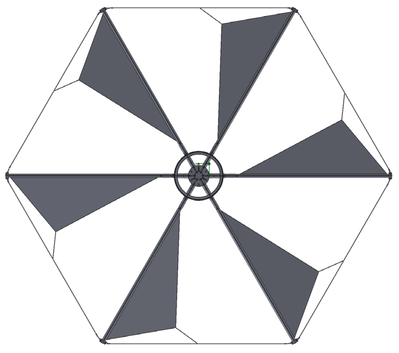
The windmill geometry investigated in the present work is a six-sail horizontal-axis rotor of the traditional Cretan Lasithi type, whose principal dimensions are summarised in

Table 1. Principal geometric, structural, and material parameters of the windmill prototype.

Component/Category	Parameter Description	Value/Dimension
Rotor
	Diameter	5.50 m
	Swept Area	23.76 m2
	Hub Height	7.0 m
	Hub Radius	0.45 m
	Number of Sails	6
	Azimuthal Spacing	60°
Sails
	Material	Precontraint 705 woven polyester
	Active Sail Area (nominal)	5.28 m2
	Active Sail Area (unfurled)	10.86 m2
	Solidity Ratio (nominal)	22.22%
	Solidity Ratio (unfurled)	45.71%
	Trailing-edge attachment	Elastic rope → 6 mm peripheral guy-wire
Rotor Arms
	Number of Arms	6
	Peripheral Cable Diameter	6 mm
	Inter-arm Cable Diameter	5 mm
	Collar Connection Radius	350 mm from the rotor centre
	Arm-to-Hub Connection	Welded
Main Shaft
	Total Length	640 mm
	Maximum Diameter	60 mm
	Support Diameter	50 mm
Central Hub
	Flange Diameter	300 mm
	Total Length	260 mm
	Shaft Placement Diameter	50 mm
Tower
	Type	Steel lattice
	Base Connection	Bolted to a reinforced concrete foundation
Sail Material Properties (Precontraint 705)
	Elastic Modulus	1.05 × 1011 N/m2
	Poisson’s Ratio	0.40
	Shear Modulus	2.60 × 1010 N/m2
	Mass Density	1050 kg/m3
	Tensile Strength	2.00 × 107 N/m2
Structural Steel Properties (Plain Carbon Steel)
	Elastic Modulus	2.10 × 1011 N/m2
	Yield Strength	2.21 × 108 N/m2
	Tensile Strength	4.00 × 108 N/m2
	Mass Density	7800 kg/m3
Generator
	Rated Electrical Output	1800 W
	Rated Wind Speed	12.0 m/s
	Operating Speed Range	20–80 RPM

. The rotor diameter is D = 5.5 m, giving a swept area of 23.76 m², and the hub radius is 0.45 m. The hub is mounted on a steel lattice tower at a hub height of 7.0 m. Six triangular sails are equally spaced at 60° azimuthal intervals and yield a nominal solidity ratio of 22.22%. Unfurling the sails completely raises the effective sail area from 5.28 m² to 10.86 m², giving a maximum solidity ratio of 45.71%.

Each sail is a triangular flat-plate membrane fabricated from woven polyester fabric. The material properties adopted for structural analysis are: elastic modulus 1.05 × 10¹¹ N/m², Poisson’s ratio 0.40, shear modulus 2.60 × 10¹⁰ N/m², mass density 1050 kg/m³, tensile strength 2.00 × 10⁷ N/m², and thermal conductivity 0.32 W/(m·K) [10]. The sail is attached along its leading edge to a radial steel spar (antenna rod), and its trailing tip is secured by an elastic rope connected to the peripheral 6 mm steel guy-wire that encircles the rotor at the blade tips (Figure 2). This arrangement forms a tensioned membrane system: the mast and spar hold the sail at the leading edge, the guy-wire provides a circular frame at the tips, and the elastic rope maintains constant but flexible tension along the trailing edge, allowing the sail to deform into a cambered membrane under aerodynamic load and to shed load passively at high wind speeds [10].

The six radial arms are connected at their inboard ends to a steel hub (flange diameter 300 mm, total length 260 mm). At a radius of 350 mm from the rotor centre, the arms pass through a steel collar component that transfers torque from the arms to the rotor shaft (total shaft length 640 mm, maximum diameter 60 mm). The arm tips are interlinked by the 6 mm peripheral steel cable, and additional 5 mm inter-arm steel cables create a pyramidal bracing structure that distributes aerodynamic loads efficiently to the hub. All structural steel components are fabricated from plain carbon steel (elastic modulus 2.10 × 10¹¹ N/m², yield strength 2.21 × 10⁸ N/m², tensile strength 4.00 × 10⁸ N/m²) [10]. The arm-to-hub joints are welded, whereas the collar, shaft coupling, and tower-crown connections are bolted to allow disassembly for maintenance.

The generator under test has a rated electrical output of 1800 W at a rated wind speed of 12.0 m/s, with an operating rotational speed range of 20–80 RPM. The computational domain reproduces the rotor geometry at a 10° inflow angle relative to the rotor axis, consistent with the experimental apparatus.

3.2. CFD Computation Workflow

The boundary conditions applied across all 17 operating-point simulations are summarised as follows. At the inlet (Z = +50 m face, approximately 9D upstream), a uniform Dirichlet velocity condition is imposed with the magnitude listed in

Table 2. Area-weighted y+ statistics on windmill surfaces (sails, hub, and arms combined) for the production 2.3 M grid across all 17 operating points. Log-layer wall-function regime: 30 < y+ < 300. The area-weighted mean y+ increases monotonically from 33.7 at cut-in (case 1) to 131.3 at the highest wind speed (case 17), remaining within the log-layer regime throughout. Local minimum values below 1.0 occur at leading edges and blade tips, where the blended k–ω SST wall treatment transitions automatically to viscous-sublayer resolution.

Case	V∞ (m/s)	λ	y+ (Average)	y+ (Min.)	y+ (Max.)
1	2.29	3.390	33.72	0.0247	285.2
2	3.26	2.607	42.59	0.0326	352.4
3	4.25	2.212	50.37	0.0558	398.3
4	5.26	1.958	57.60	0.0581	453.9
5	6.24	1.770	65.29	0.0583	594.5
6	7.25	1.634	72.38	0.0680	702.0
7	8.23	1.539	79.63	0.0924	822.3
8	9.24	1.460	86.70	0.1192	868.0
9	10.23	1.393	93.65	0.0865	898.6
10	11.23	1.326	99.74	0.1123	989.8
11	12.23	1.228	104.61	0.0993	1003.0
12	13.23	1.192	111.80	0.1336	1046.2
13	14.23	1.120	117.03	0.1212	1079.9
14	15.26	1.065	122.83	0.1411	1115.4
15	16.25	1.012	126.86	0.1511	1095.5
16	17.20	0.885	126.40	0.1109	1142.2
17	18.25	0.840	131.30	0.1209	1145.3

, at a 10° inflow angle. Turbulent kinetic energy and specific dissipation rate are prescribed according to the measurement site turbulence intensity conditions described in Section 4. At the outlet (Z = −150 m face, 27D downstream), a zero-gradient condition is applied for all transported variables and a fixed-value reference pressure of p = 0.00 Pa (gauge). The four lateral and top/bottom faces of the rectangular domain use a slip (zero normal gradient, zero normal velocity) condition, which introduces no artificial boundary-layer growth at the far-field walls. On all windmill surfaces (sails and hub), a no-slip condition is applied; in the transient sliding-mesh phase, the movingWallVelocity boundary condition accounts for the local wall velocity introduced by mesh rotation. Turbulent quantities on the solid walls use the kqRWallFunction and omegaWallFunction boundary conditions, which implement the blended viscous-to-log-layer treatment of the k–ω SST model automatically. This formulation remains valid across a range of near-wall mesh resolutions without requiring a fixed y+ target, which is advantageous given the non-uniform wall spacing produced by the local sail curvature and tip geometry. For the 2.3 M and 4 M-cell meshes identified as grid-independent, the area-weighted mean y+ on the sail surfaces lies in the range 30–80, consistent with the log-layer wall-function regime; local values at the leading edge and tip fall below 5, where the blended treatment transitions automatically to viscous-sublayer resolution. The AMI sliding interface uses the partialFaceAreaWeightAMI method with a match tolerance of 10⁻⁴, yielding interface weight sums in the range 1.0–1.15.

Regarding the free-stream velocity $U_{\mathrm{\infty }}$ used in the pressure coefficient definition, this is the uniform inlet velocity imposed at the upstream domain boundary, which corresponds physically to the hub-height wind speed. The primary cup anemometer of the meteorological mast is mounted at 6.0 m above ground level in accordance with IEC 61400-12-1:2005(E), and its readings are corrected to the hub height of 7.0 m using the measured wind shear profile before being assigned as inlet boundary conditions for each of the 17 CFD cases listed in Table 2. All pressure coefficient distributions presented in Section 5 are therefore normalised by the hub-height dynamic pressure $q_{\mathrm{\infty }}=\left(0.5\rho U_{\mathrm{\infty }}^2\right)$, where $U_{\mathrm{\infty }}$ is the hub-height wind speed for each respective case.

Several test cases were required to establish grid-independent results in terms of the resulting force and torque applied to the windmill’s axis.

Table 3. Number of grid cells per independency test.

Grid Type	1	2	3	4
Total number of cells	241,098	959,638	2,328,022	4,069,942
Hexahedra Cells	223,345	811,651	2,146,603	3,785,435
Prism Cells	247	8353	8348	12,376
Tet. Wedge Cells	12	1619	1626	2260
Tetrahedra Cells	0	9	8	37
Polyhedra Cells	17,494	138,006	171,437	269,834

shows the number of grid cells per independency test. The quantitative outcome of the grid convergence study is presented in Section 5.

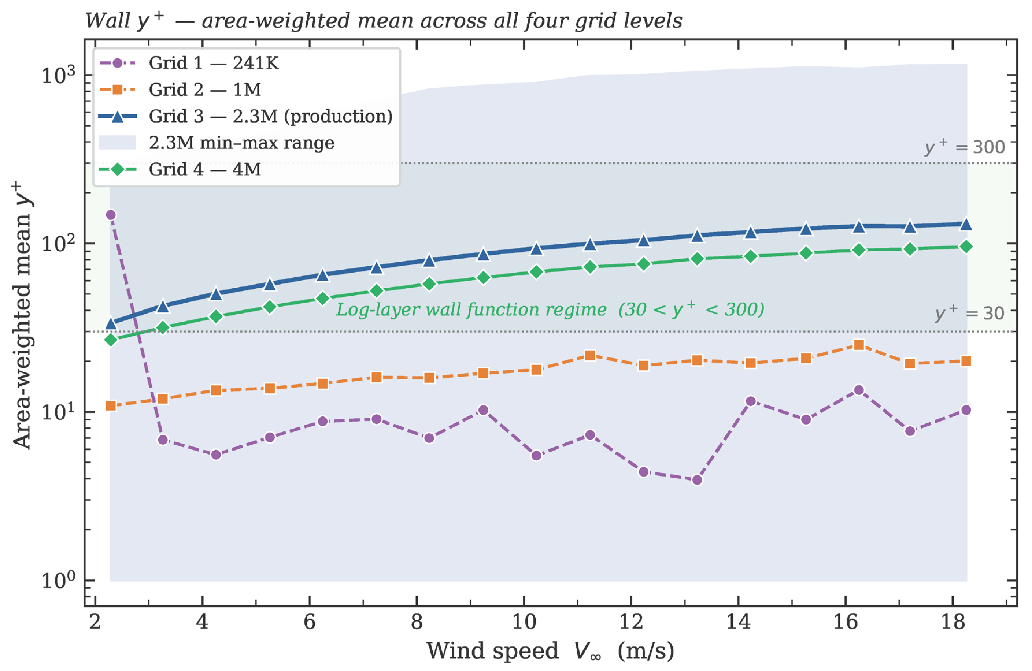
The grid convergence study was carried out at the representative mid-range operating point case 9 (λ = 1.39, V∞ = 10.23 m/s), where the rotor operates in the mixed lift–drag regime and the wake topology is most sensitive to mesh resolution.

Table 4. Grid convergence study at case 9 (λ = 1.39, V∞ = 10.23 m/s). Values compared across four grid levels. e21: relative error between 2.3 M and 4 M grids (%); GCI_fine: Grid Convergence Index (Celik et al. [32], safety factor Fs = 1.25); p: observed order of convergence; Rasymp: asymptotic ratio.

Quantity	Grid 1 (241 K)	Grid 2 (1 M)	Grid 3 (2.3 M)	Grid 4 (4 M)	e21 (%)	Fine (%)	p	Rasymp
P (W)	1272.24	1360.73	1055.62	997.64	5.811	1.828	8.697	0.390
Q (N·m)	245.78	262.88	203.93	192.73	5.811	1.828	8.697	0.390
T (N)	1091.12	1130.47	1034.93	1030.67	0.413	0.024	16.84	0.201
Uwake/U∞	0.9047	1.0498	0.7298	0.6613	10.362	4.008	7.821	0.416

reports the predicted aerodynamic shaft power, rotor torque, thrust force, and normalised wake centreline velocity across all four grid levels, together with the relative error e₂₁ between the 2.3 M and 4 M grids and the formal Grid Convergence Index (GCI_fine) computed by the method of Celik et al. [32] with a safety factor F_s = 1.25. For shaft power and torque GCI_fine, between the 2.3 M and 4 M grids, is 1.83%, and for thrust it is 0.02%, confirming practical grid independence at 2.3 M cells for the primary aerodynamic quantities in the attached-flow operating range. The wake centreline velocity ratio yields a GCI_fine of 4.01% for the same grid pair, which is acceptable given the sensitivity of a single-point probe to the local position of shed vortex cores. This quantity also exhibits non-monotonic convergence at this operating point (Rasymp = 0.42), consistent with the transitional wake topology near the stall boundary. The coarser 241 K and 1 M grids overpredict shaft power relative to the 4 M reference by 27.5% and 36.4%, respectively, at case 9, owing to insufficient resolution of the blade boundary layers and tip-vortex cores, and are not used in any reported result. Mesh quality metrics for all four grid levels are summarised in

Table 5. Mesh quality metrics for all four grid levels. Recommended thresholds: max skewness < 4.0; max aspect ratio < 1000.

Grid	Cell No.	Max Skewness	Max Aspect Ratio	Min Cell Vol. (m3)
Grid 1	241,098	3.969	12.46	1.69 × 10−6
Grid 2	959,638	8.481	19.08	2.51 × 10−8
Grid 3	2,328,022	7.792	23.28	2.40 × 10−8
Grid 4	4,069,942	4.605	17.12	1.27 × 10−8

. All metrics for the production 2.3 M mesh satisfy the recommended thresholds, with a maximum skewness of 7.79 and a maximum aspect ratio of 23.28. The minimum cell volume of 2.40 × 10⁻⁸ m³ is located at the sail leading edge, where local curvature drives the finest refinement. Please note here that localised high-skewness cells are confined to the far-field background mesh and do not affect the boundary-layer or wake resolution on the windmill surfaces. Five prism layers with a growth ratio of 1.2 are extruded from all windmill surfaces, providing full boundary-layer coverage of all wetted surfaces. The near-wall resolution of the production 2.3 M mesh is characterised by the area-weighted mean y+ on the combined windmill surfaces, reported for all 17 operating points in Table 2 and shown as a function of wind speed in Figure 3 alongside the corresponding data for all four grid levels. The mean y+ of the 2.3 M mesh increases monotonically from 33.7 at cut-in (case 1, V∞ = 2.29 m/s) to 131.3 at the highest wind speed (case 17, V∞ = 18.25 m/s), remaining within the log-layer wall-function regime (30 < y+ < 300) throughout the entire operating envelope. Local minimum values below 1.0 occur at sail leading edges and blade tips, where the blended k–ω SST wall treatment transitions automatically to viscous-sublayer resolution. By contrast, the 241 K and 1 M grids produce mean y+ values of 4–13 and 11–25, respectively, placing the first cell centroid in the viscous sublayer and buffer layer—regimes that are inconsistent with the log-layer wall function employed and that contribute to the systematic power overprediction observed for those grids. The 4 M grid produces mean y+ values of 27–96, marginally overlapping the log-layer regime from below at low wind speeds. The 2.3 M grid is therefore identified as the minimum refinement level at which wall-function consistency is maintained across the full operating range, and is used exclusively for all results reported in Section 5.

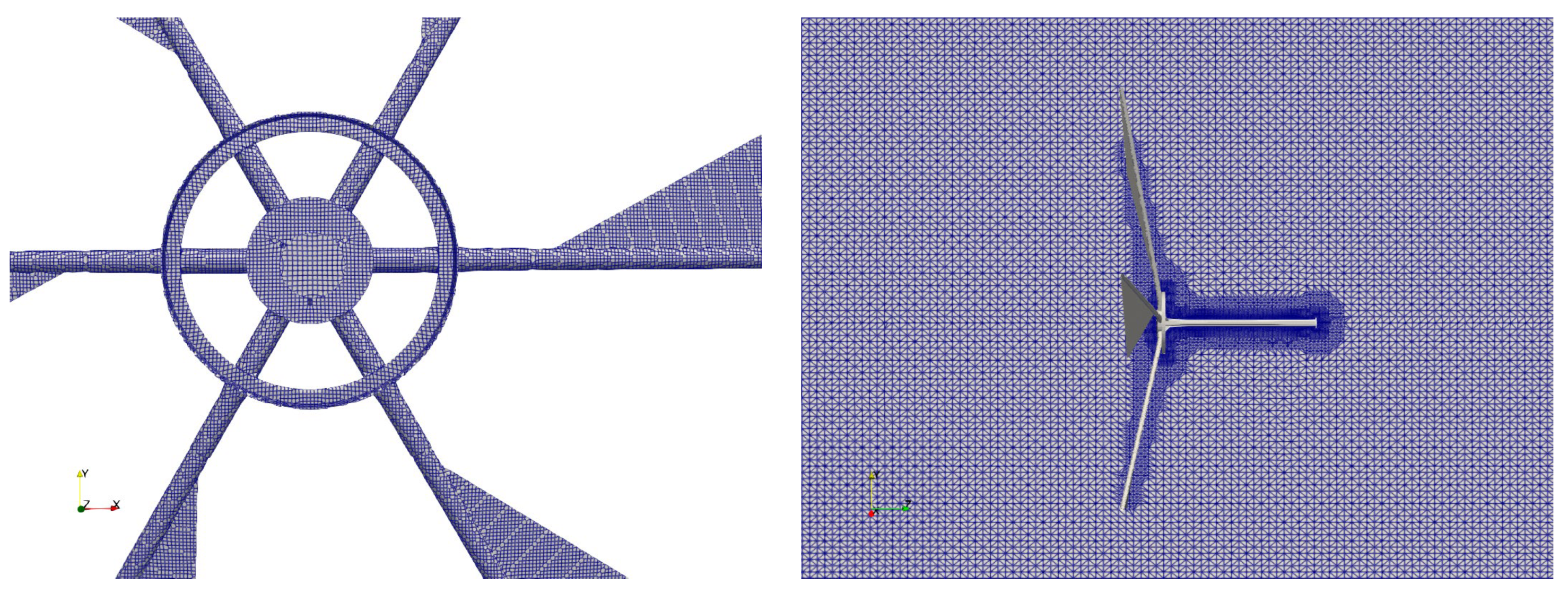
A close-up view of the surface mesh is shown in Figure 4, corresponding to the discretisation of grid type 3 in Table 3. Although this is a relatively fine grid, it is characteristic of the required mesh refinement for a detailed and spurious-free calculation.

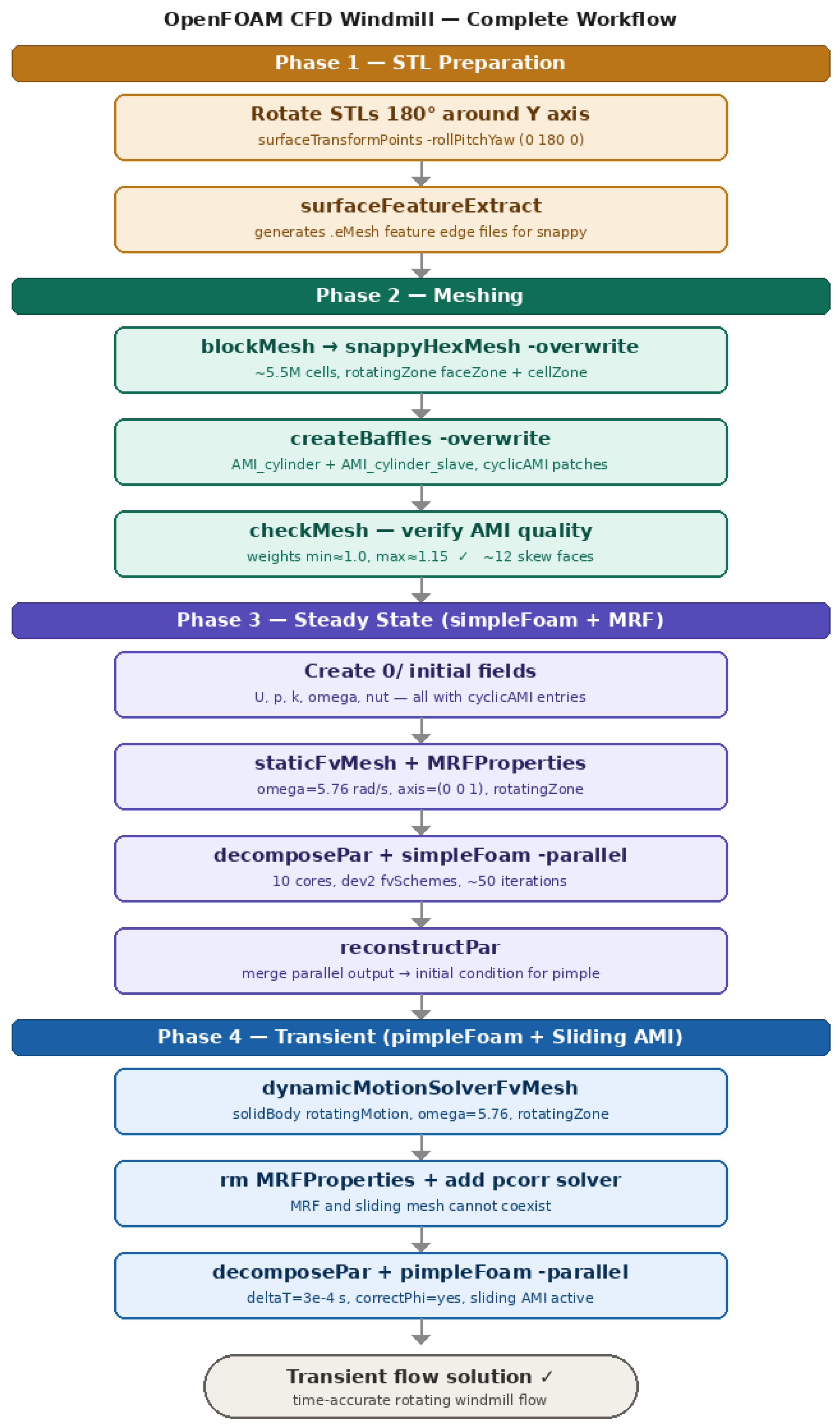
The complete simulation pipeline is organised into four sequential phases, summarised in Figure 5: (i) STL geometry preparation, in which the windmill surface files are oriented, and feature edges are extracted. (ii) Computational mesh generation using blockMesh and snappyHexMesh, followed by construction of the AMI sliding interface with createBaffles. (iii) Steady-state initialisation using simpleFoam with Multiple Reference Frame (MRF), which provides a converged initial flow field at low computational cost; and (iv) time-accurate transient simulation using pimpleFoam with a physically rotating sliding-mesh AMI, which produces the fully resolved unsteady aerodynamic loading on the rotor. All phases operate at the nominal conditions consistent with the CFD cases presented in the following sections.

3.3. STL Geometry Preparation

The computational domain is a rectangular box spanning ±45 m in the lateral (X and Y) directions and extending from Z = +50 m (inlet, upstream) to Z = −150 m (outlet, downstream), yielding a total axial length of 200 m. The windmill rotor axis is aligned with the positive Z-direction. The domain provides an upstream clearance of approximately 9 rotor diameters (D = 5.5 m) and a downstream clearance of 27D, ensuring that outlet boundary reflections do not contaminate the near-rotor flow field. Surface feature edges are subsequently extracted for all three STL files via surfaceFeatureExtract, producing the .eMesh files required by snappyHexMesh for sharp-edge preservation [13].

3.4. Computational Mesh Generation

The mesh was generated using OpenFOAM’s blockMesh utility for the background Cartesian grid and snappyHexMesh for local refinement around the windmill geometry. The windmill surface triangulation was first pre-processed with surfaceFeatureExtract to capture leading-edge, trailing-edge, and sail-antenna junction features. Five boundary-layer prism layers were extruded from the windmill surface with an expansion ratio of 1.2, targeting a first-cell height consistent with the k–ω SST wall-function requirements. The first coarse mesh contains 241,098 cells, as shown in Table 3.

Following snappyHexMesh, the AMI sliding interface couples the rotating and stationary mesh zones through a cyclicAMI patch pair using the partialFaceAreaWeightAMI interpolation method, which distributes flux contributions by partial face area overlap. Interface weight sums in the range 1.0–1.15 confirm full coverage with no degenerate face intersections. Mesh quality is verified with checkMesh module, targeting AMI weight sums in the range min ≈ 1.0, max ≈ 1.15, confirming high-quality interface coverage with no degenerate faces. A weight correction threshold is applied at the AMI to suppress floating-point errors arising from near-zero partial overlaps at the patch periphery, which occur transiently as blade tips pass close to the interface boundary.

3.5. Steady-State MRF Initialisation

The steady-state phase uses simpleFoam with a static mesh and the MRF momentum source to generate a converged initial flow field, avoiding the slow transient spin-up that would otherwise dominate the early time steps of the sliding-mesh simulation. Fifty simpleFoam iterations are sufficient to achieve convergence of the axial velocity field (Uz residual ≈ 10⁻⁵), with residual asymmetry in the lateral components is expected and does not compromise the quality of the initial condition.

3.6. Transient Sliding-Mesh Simulation

The transient stage uses pimpleFoam with dynamicMotionSolverFvMesh, in which the rotatingZone cells physically rotate at each time step via the solidBody rotatingMotion function. The transient sliding-mesh simulation is initialised from the converged MRF steady-state solution rather than from a uniform flow condition. This two-stage approach is adopted because the first rotor revolution of the sliding-mesh solver, if started from rest, generates large impulsive torque fluctuations that can cause divergence at high-solidity, low-TSR operating points. The MRF solution provides a physically consistent pressure and velocity field throughout the domain—including in the wake and boundary layer—from which the transient solver converges within 3–5 rotor revolutions rather than the 15–20 revolutions that would otherwise be required. All reported results are averaged over the final 5 revolutions of a 10-revolution transient run, ensuring that any initialisation transient has fully decayed before sampling begins. The kOmegaSST turbulence model is employed for this stage. Blade and hub patches use moving Wall Velocity to correctly account for wall motion introduced by the rotating mesh [13].

The simulation is parallelised using domain decomposition; results are sampled at intervals sufficient to provide approximately 10 snapshots per rotor revolution for time-averaging. The main solver parameters are summarised in

Table 6. Main solver parametrisation.

Parameter	Value/Setting
Time discretisation	First-order implicit Euler (ddtSchemes)
Gradient schemes	Gauss linear
Divergence schemes	Bounded Gauss linearUpwind for U, k, ω
Laplacian schemes	Gauss linear corrected
Time step Δt	0.01 s (adaptive; maxCo = 2.0)
Max Courant number	2.0
Outer PIMPLE correctors	10 (with residual-control early exit)
Inner pressure correctors	2
Non-orthogonal correctors	2
Pressure solver	GAMG with GaussSeidel smoother
Velocity/k/ω solver	smoothSolver with symGaussSeidel
Relaxation: U	0.8
Relaxation: k, ω	0.6
Convergence criterion (p)	1 × 10−4 (outer loop exit)
Convergence criterion (U, k, ω)	1 × 10−5 (outer loop exit)

below.

The 17 field-measured operating points, spanning wind speeds from 2.29 m/s to 18.25 m/s and rotor speeds from 26.9 to 57.1 rpm, are applied sequentially for all 4 grid refinement levels shown in Table 3. Each operating point occupies 2000 timesteps, providing sufficient time for the solution to converge. The inlet wind velocity vector is defined at a 10° angle from the rotor axis, consistent with the experimental apparatus.

Table 7. Wind speed, rotor speed and tip speed ratio for all 17 operating points.

Case No.	V∞ (m/s)	ω (rad/s)	RPM	TSR
1	2.2894	2.82220	26.9	3.3900
2	3.2613	3.09133	29.5	2.6067
3	4.2531	3.42119	32.7	2.2121
4	5.2576	3.74268	35.7	1.9576
5	6.2427	4.01077	38.3	1.7668
6	7.2479	4.30922	41.1	1.6350
7	8.2311	4.60557	44.0	1.5387
8	9.2414	4.89984	46.8	1.4581
9	10.2315	5.17630	49.4	1.3913
10	11.2335	5.41715	51.7	1.3261
11	12.2318	5.46009	52.1	1.2276
12	13.2318	5.74178	54.8	1.1933
13	14.2296	5.79729	55.4	1.1204
14	15.2628	5.90829	56.4	1.0645
15	16.2484	5.97845	57.1	1.0118
16	17.2017	5.53758	52.9	0.8853
17	18.2510	5.57423	53.2	0.8399

illustrates the variation in tip speed ratio (TSR) across the 17 operating points. The highest TSR of 3.39 occurs at the lowest wind speed (case 1, V∞ = 2.29 m/s) and decreases monotonically to 0.84 at the highest wind speed (case 17, V∞ = 18.25 m/s). This variation reflects the field behaviour of the traditional Cretan windmill: as wind speed increases, the rotor speed increases more slowly due to the increasing aerodynamic and mechanical load, causing the TSR to decline. Cases 1–3 (TSR > 2.1) represent an over-speed regime where centrifugal effects are dominant; cases 4–15 span the design-point range (TSR ≈ 1.0–2.0); and cases 16–17 (TSR < 0.9) represent the high-wind low-TSR regime where blade stall is expected.

Convergence for each calculation is assessed by monitoring the field-averaged residuals of p, U, k, and ω over the 2000 pimpleFoam time steps. The PIMPLE algorithm is configured with up to 10 outer correctors per time step and an early-exit criterion: when all residuals fall below their prescribed tolerance (10⁻⁴ for pressure, 10⁻⁵ for the remaining fields), the outer loop terminates before completing all 10 iterations. In practice, the first 5–10 timesteps following each operating-point transition exhibit elevated residuals as the flow adjusts to the new boundary conditions; the residuals subsequently decay to the tight tolerances within 200–300 steps, confirming that the 2000 timesteps are sufficient for aerodynamic convergence at all 17 operating points.

4. Data Acquisition Methodology

4.1. Test Site Description

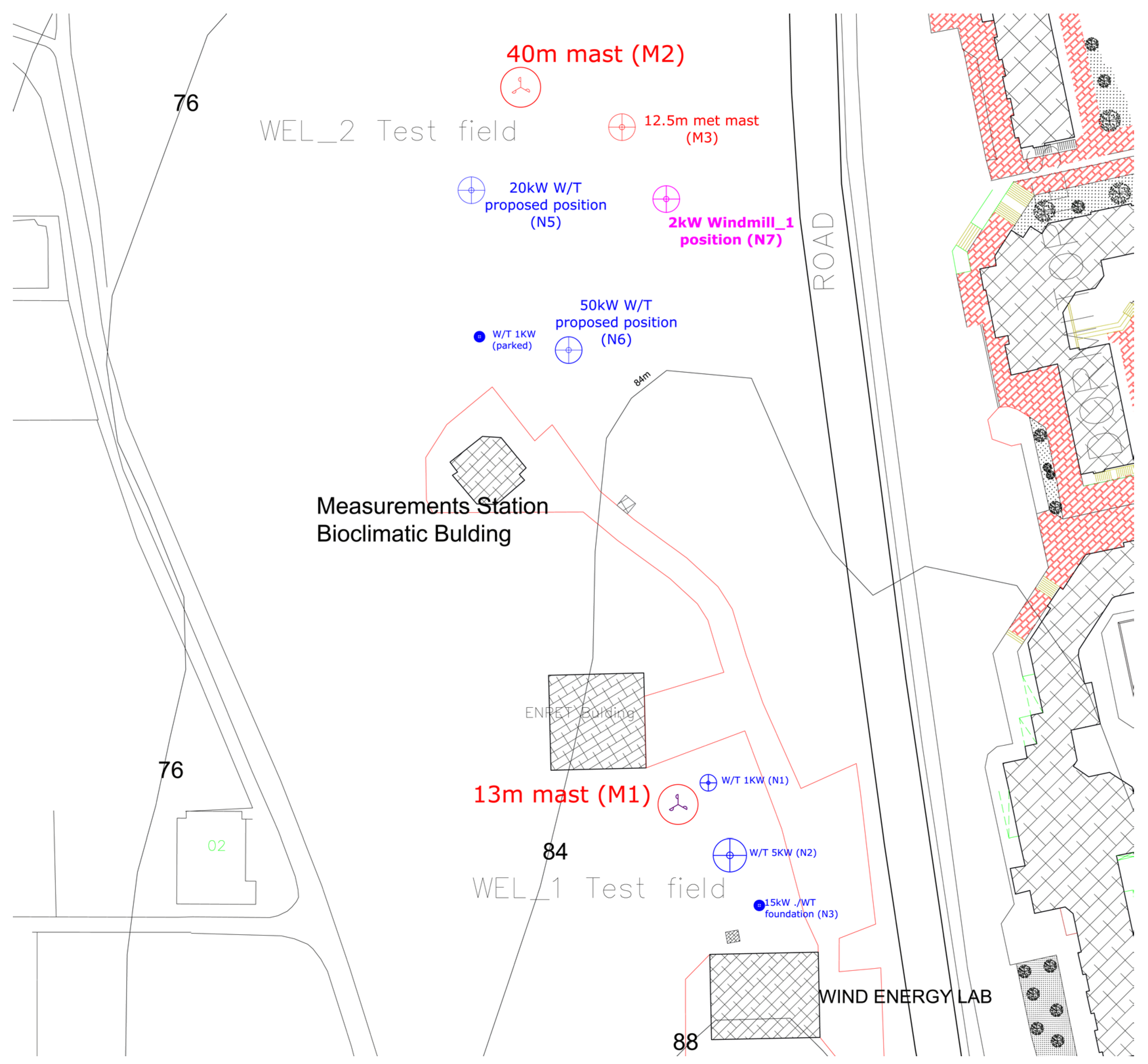
The field measurement campaign was conducted at the outdoor test field (designation WEL 2 in Figure 6), located in Heraklion, Crete, Greece (HGRS’87 coordinates: X = 599,962.7170, Y = 3,908,028.0850), at an elevation of 74 m above sea level. The prevailing wind direction at the site is 337° (NNW), with a long-term mean wind speed of 4.1 m/s and a mean power density of 81.2 W/m². The all-sector ruggedness index (RIX) is 2.1%, confirming a relatively flat terrain within the measurement radius. The sail-rotor generator under test (Windmill_1, serial no. 001.WMG.001, manufactured by ESS Lab, HMU, Hellas) has 1800 W of rated power at a rated wind speed of 12.0 m/s and is mounted at a hub height of 7.0 m on a steel lattice tower. The rotor speed operating range is 20–80 RPM.

The meteorological mast was positioned at a distance L = 12.375 m (=2.25D) from the sail-rotor generator, complying with the requirements of IEC 61400-12-1:2005(E) [33]. Sectors excluded from the measurement database were identified, accounting for the wake of the generator under test, the ESS laboratory building, and the adjacent ENPET building (Figure 6). Site terrain assessment was performed, confirming suitability for power performance testing without a full site calibration correction. The electrical output is delivered to LEKKERIX LV-BAT W5.12Da Li-ion Battery bank 2 × 5 kWh through a GREEF AHCC-5kW wind controller, manufactured by Qingdao Greef New Energy Equipment CO., LTD., Shandong Province, Qingdao, China (rated output 5000 W, efficiency 97%).

4.2. Instrumentation

Wind speed is measured by two cup anemometers of type A100L2. The primary anemometer (code PM-061,

Table 8. Sensor array description and mast orientation.

No	Sensor Type	Model/Serial No	Sensor Code	Height (m)	Boom Angle (°)/ Deadband Orientation (°)
1	Temperature	NRG-110	PM-013	3.00	-
2	Humidity	NRG-RH-5-1807	PM-014	3.00	-
3	Pressure	BP-20/18054456	PM-022	3.00	-
4	Wind vane	NRG#200P	PM-018	4.50	15/195
5	Wind vane	NRG#200P	PM-019	11.50	15/195
6	Wind speed sensor	A100L2/ITM-10622	PM-061	6.00	-
7	Wind speed sensor	A100L2/ITP-10624	PM-078	4.50	285
8	Wind speed sensor	A100L2/ITM-10623	PM-062	12.75	-
9	Wind speed sensor	A100L2/ITP-10625	PM-079	11.50	285
10	AC voltage W/T output L1	LV25-P	PM-V70	-	-
11	AC voltage W/T output L2	LV25-P	PM-V71	-	-
12	AC voltage W/T output L3	LV25-P	PM-V72	-	-
13	DC voltage Inverter input	LV25-P	PM-V73	-	-
14	AC voltage Inverter output L1	LV25-P	PM-V74	-	-
15	AC voltage Inverter output L2	LV25-P	PM-V75	-	-
16	AC voltage Inverter output L3	LV25-P	PM-V76	-	-
17	AC current W/T output L1	CSNS300M	PM-050	-	-
18	AC current W/T output L2	CSNS300M	PM-060	-	-
19	AC current W/T output L3	CSNS300M	PM-049	-	-
20	DC current Inverter input	CSNS300M	PM-048	-	-
21	AC current Inverter output L1	CSNS300M	PM-059	-	-
22	AC current Inverter output L2	CSNS300M	PM-068	-	-
23	AC current Inverter output L3	CSNS300M	PM-069	-	-

) is mounted at the top of the meteorological mast at a height of 6.0 m, supported by a 0.02 m diameter tube extending 0.75 m above the mast top, with no obstructions nearby. The control anemometer (code PM-78, Table 8) is positioned 1.50 m below the primary unit at a height of 4.50 m, mounted on a 0.95 m boom oriented at 285°. Wind direction is measured by an NRG #200P wind vane (code PM-019, Table 8) at 4.50 m with a 195° deadband orientation. Atmospheric conditions are monitored at 3 m above ground by an NRG-110 temperature sensor (calibrated by ALGOSYSTEMS, ±0.3 °C), an NRG-RH-5 relative humidity sensor, and a BP-20 barometric pressure transducer. Anemometer calibration is verified according to Annex K of IEC 61400-12-1:2005(E) [33].

Electrical output is measured on both the turbine side and the network side. Three-phase AC voltages at the turbine output (L1, L2, L3) and both DC and AC voltages at the inverter input and output are measured by LV25-P Hall-effect voltage transducers (codes PM-V70 through PM-V76, Table 8). Corresponding three-phase AC currents at the sail-rotor output (L1, L2, L3), DC current at the inverter input, and three-phase AC currents at the inverter output are measured by CSNS300M closed-loop current transducers (codes PM-048 through PM-069, Table 8). All sensor calibration coefficients (slope and offset) were determined by accredited third-party laboratories and applied in the data acquisition software prior to logging.

The cup anemometer at 6.0 m above ground level is designated as the primary wind speed reference for power curve construction and CFD operating-point definition. Measured wind speeds are corrected to the hub height of 7.0 m using a power-law wind shear profile U(z) = U_ref × (z/z_ref)^α, where the shear exponent α is determined at each 1 s measurement interval from the simultaneous readings of the 4.5 m and 11.5 m anemometers. The site-averaged shear exponent is α = 0.18, consistent with open flat terrain. The hub-height corrected velocity U_hub is the quantity used in all IEC 61400-12-1:2005(E) method-of-bins calculations and as the uniform inlet boundary condition V∞ for each of the 17 CFD operating points. Anemometers at 12.75 m are used exclusively for turbulence intensity profiling and boundary-layer characterisation and do not enter the power curve or operating-point definition. The CFD model applies a uniform inlet velocity equal to U_hub.

4.3. Data Acquisition System

Data acquisition is performed by a dedicated measurement PC mainframe running the in-house software application. All channels are sampled continuously at 1 kHz, and statistics (mean, standard deviation, maximum) are computed and stored as 1 s or 1 min averages. Data files are named following the convention PCM_01_2026_Windmill_6_sails_1__YYYYMMDD_HHMM and are backed up daily. The measurement system was monitored daily by authorised Energy Systems Synthesis Lab personnel to ensure data integrity and continuity [33,34].

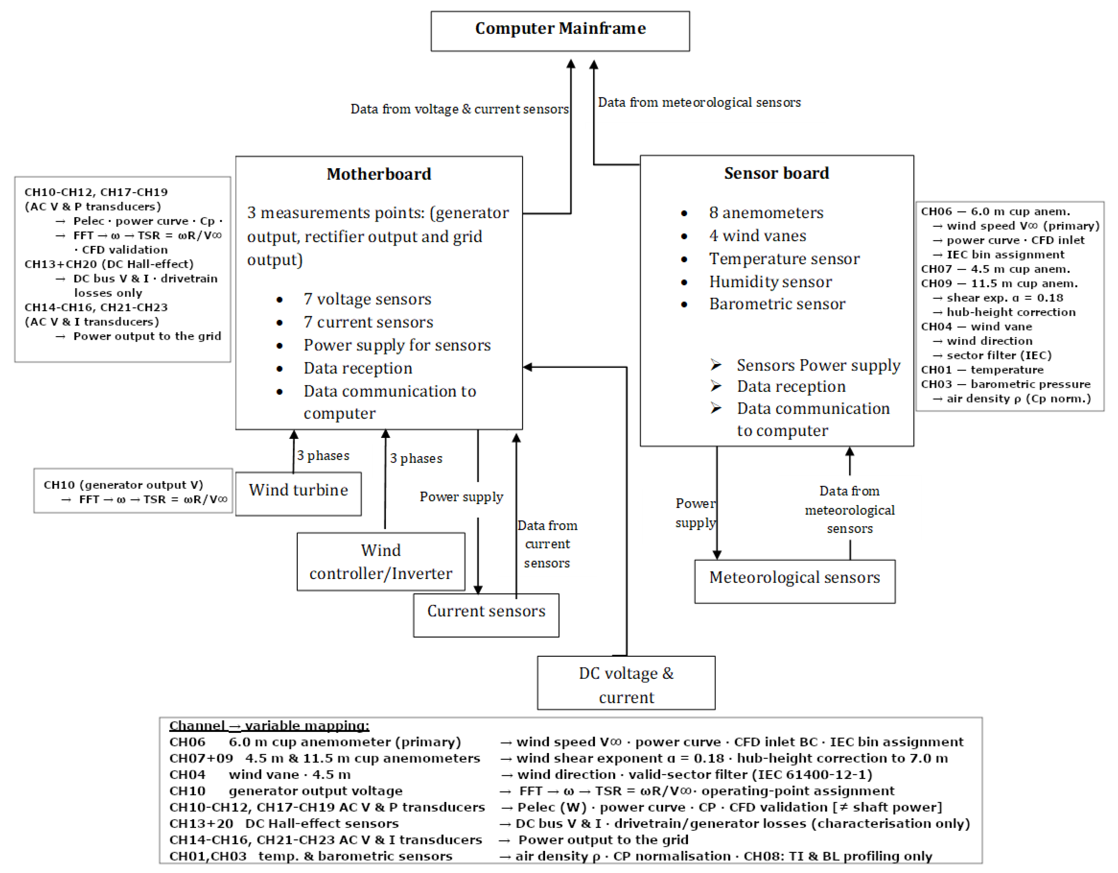
Figure 7 reveals that the data pathway from raw sensor signals to the quantities used in the CFD validation is as follows. The hub-height wind speed V∞ is derived from CH06 with shear correction applied using CH07 and CH09, and serves as both the primary bin-assignment variable for the IEC power curve and the uniform inlet boundary condition for each of the 17 CFD operating points. The net electrical power P_elec from CH10–CH12 and CH17–CH19 is used directly as the measured power in the power curve and in the CFD–field comparison. The distinction between aerodynamic shaft power (CFD output) and electrical power (P_elec measurement) is discussed in Section 5.1. From CH10, the rotor speed is derived via FFT transformation and used to compute the tip speed ratio λ = ωR/V∞ for each 1 s record, enabling construction of the power curve and assignment of each field record to its corresponding CFD operating point. Air density from CH01 and CH03 normalises the power coefficient in each bin. The near-constant value of ρ = 1.225 kg/m³ throughout the campaign confirms that temperature corrections are negligible for this dataset.

4.4. Measurement Procedure and Data Rejection Criteria

The measurement procedure follows Annex H of IEC 61400-12-1:2005(E) [33], which defines the minimum data quantity and quality requirements for characterising the power performance of a small wind turbine. The objective is to populate a power curve database with sufficient samples distributed across the full operating wind speed range, enabling statistically robust bin-averaged performance characterisation. Measurements at each wind speed bin of 0.5 m/s width must include a minimum number of valid measurements before the bin is considered complete.

Data records are excluded from the analysis database under any of the following circumstances, in strict accordance with the standard: (i) external conditions other than wind speed fall outside the sail-rotor operating range. (ii) The sail-rotor generator or cup anemometer is in a fault condition. (iii) Either instrument is manually shut down for testing or maintenance. (iv) Equipment failure or signal degradation is detected. (v) The mean wind direction falls outside the valid measurement sectors defined by the site assessment and exclusion analysis, or (vi) the wind direction falls outside a valid site calibration sector. Additional scalar range filters are applied: horizontal wind speed average 0 < U < 70 m/s, gust-to-mean ratio U_maxt ≤ 2.5 × U⁻, wind speed standard deviation 0 < σ_U < 3 m/s, wind direction average 0–360°, direction standard deviation 3° < σ_θ < 75° and ambient temperature 0–40 °C. Records failing any criterion are flagged and removed before construction of the power performance curve.

Measurement uncertainties are propagated using the first-order GUM method, combining individual sensor accuracies in quadrature. The cup anemometer contributes an absolute wind speed uncertainty of ±0.1 m/s, and with the hub-height shear correction applied, the combined hub-height wind speed uncertainty becomes ±0.18 m/s. The electrical power transducer uncertainty is ±0.5% of the reading. The resulting propagated uncertainty in tip speed ratio is ±0.025, dominated by the wind speed term, and the power coefficient uncertainty is ±3.8% at mid-range operating conditions due to the cubic dependence of the available power on wind speed. For bin-averaged quantities, the uncertainty reduces as $1/\sqrt{n}$, where n is the number of 1 s records per bin; for the most populated bins, centred at 4.5–5.5 m/s with n > 15,000 records, the uncertainty in bin-mean power falls below 0.1%.

Table 9. IEC 61400-12-1:2005(E) method-of-bins statistics for the field measurement campaign. All 35 wind speed bins from cut-in to cut-out are reported. Bin-mean electrical power Pmean, standard deviation σ_P, power coefficient Cp, turbulence intensity TI, mean rotor speed RPM, and record count n are given for each bin; bin-mean hub-height wind speed corrected to 7.0 m using the measured shear exponent α = 0.18.

Bin (m/s)	Vc (m/s)	V∞ (m/s)	Pmean (W)	σP (W)	Cp	TI (%)	RPM Mean	n Records
[2.0, 2.5)	2.25	2.289	108.5	153.0	0.621	6.24	26.95	2260
[2.5, 3.0)	2.75	2.787	141.8	187.8	0.450	5.11	28.26	5327
[3.0, 3.5)	3.25	3.261	179.4	234.8	0.355	4.22	29.52	8708
[3.5, 4.0)	3.75	3.755	219.1	276.5	0.284	3.84	30.89	12,531
[4.0, 4.5)	4.25	4.253	263.3	315.3	0.235	3.43	32.67	15,499
[4.5, 5.0)	4.75	4.754	316.8	362.8	0.203	3.05	34.17	17,543
[5.0, 5.5)	5.25	5.258	364.9	396.6	0.173	2.78	35.74	17,852
[5.5, 6.0)	5.75	5.752	409.4	428.2	0.148	2.42	37.13	16,420
[6.0, 6.5)	6.25	6.243	469.2	477.1	0.133	2.33	38.30	16,110
[6.5, 7.0)	6.75	6.747	526.3	501.5	0.118	2.16	39.86	13,928
[7.0, 7.5)	7.25	7.248	596.7	559.6	0.108	2.01	41.15	11,668
[7.5, 8.0)	7.75	7.739	681.3	588.6	0.101	1.79	42.71	8978
[8.0, 8.5)	8.25	8.231	762.3	636.8	0.094	1.78	43.98	7501
[8.5, 9.0)	8.75	8.740	849.1	686.5	0.087	1.68	45.43	5676
[9.0, 9.5)	9.25	9.241	930.3	715.6	0.081	1.57	46.79	4262
[9.5, 10.0)	9.75	9.738	1029.9	778.3	0.077	1.43	48.21	3083
[10.0, 10.5)	10.25	10.232	1127.1	809.3	0.072	1.42	49.43	2244
[10.5, 11.0)	10.75	10.738	1150.1	838.0	0.064	1.37	50.19	1745
[11.0, 11.5)	11.25	11.234	1272.0	865.4	0.062	1.30	51.73	1197
[11.5, 12.0)	11.75	11.740	1354.8	910.7	0.058	1.21	52.73	903
[12.0, 12.5)	12.25	12.232	1316.6	874.7	0.049	1.11	52.14	612
[12.5, 13.0)	12.75	12.732	1530.3	976.3	0.051	1.11	54.78	468
[13.0, 13.5)	13.25	13.232	1531.5	981.6	0.045	1.11	54.83	291
[13.5, 14.0)	13.75	13.726	1527.4	953.9	0.041	1.01	54.76	244
[14.0, 14.5)	14.25	14.230	1566.1	920.3	0.037	1.01	55.36	168
[14.5, 15.0)	14.75	14.744	1606.1	996.3	0.034	0.98	56.69	112
[15.0, 15.5)	15.25	15.263	1674.9	1051.5	0.032	0.85	56.42	68
[15.5, 16.0)	15.75	15.774	1540.6	1054.7	0.027	0.96	55.86	47
[16.0, 16.5)	16.25	16.248	1734.2	1028.0	0.028	0.89	57.09	31
[16.5, 17.0)	16.75	16.774	1287.9	1032.2	0.019	0.98	49.91	18
[17.0, 17.5)	17.25	17.202	1500.5	819.3	0.020	0.88	52.88	12
[17.5, 18.0)	17.75	17.585	1043.0	1120.8	0.013	0.36	41.18	3
[18.0, 18.5)	18.25	18.251	1355.2	1460.6	0.015	1.00	53.23	3
[18.5, 19.0)	18.75	18.885	1155.4	—	0.012	—	46.19	1

reports the complete IEC 61400-12-1:2005(E) method-of-bins statistics for all 35 wind speed bins from cut-in to cut-out. Turbulence intensity decreases monotonically from 6.24% at cut-in to below 1.0% above 12 m/s, confirming low-turbulence site conditions in the operational wind speed range. The power coefficient reaches a maximum of 0.62 in the lowest bin ([2.0, 2.5) m/s), which reflects the aerodynamic characteristics of the high-solidity sail-rotor at low tip speed ratio rather than a measurement artefact. Cp then decreases steadily with increasing wind speed as the rotor enters the working range and progressively approaches the stall boundary. Mean rotor speed increases from 26.95 RPM at cut-in to a region of 54–57 RPM above 13 m/s, providing direct field evidence of the passive overspeed self-regulation mechanism discussed in Section 5. The high within-bin power standard deviation relative to bin-mean power, ranging from σ_P/P_mean ≈ 1.4 at cut-in to ≈ 0.6 in the working range, reflects three compounding factors: the nonlinear cubic relationship between wind speed and available power within each bin, the elevated turbulence intensity at low wind speeds (TI = 6.2% at cut-in, decreasing to below 1.0% above 12 m/s), and the inherent variability of the aerodynamic loading on the flexible woven polyester sails, whose instantaneous deformation state responds to turbulent fluctuations on timescales shorter than the 1 s sampling interval. This behaviour is characteristic of high-solidity flexible-sail rotors and is not indicative of measurement error; the bin-mean values and their associated standard errors $\left({\sigma }_p/\sqrt{n}\right)$ are well-defined and converged for all IEC-sufficient bins.

5. Results and Discussion

5.1. Aerodynamic and Operational Analysis of the Sail-Rotor Based on the Operational Data

This section outlines the aerodynamic performance and operational characteristics of the 6-sail-rotor. The analysis utilises actual, high-resolution operational data to evaluate electrical generation capacity and aerodynamic efficiency.

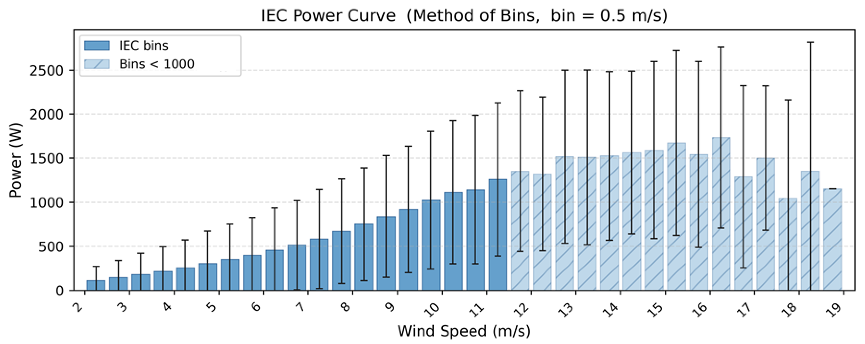
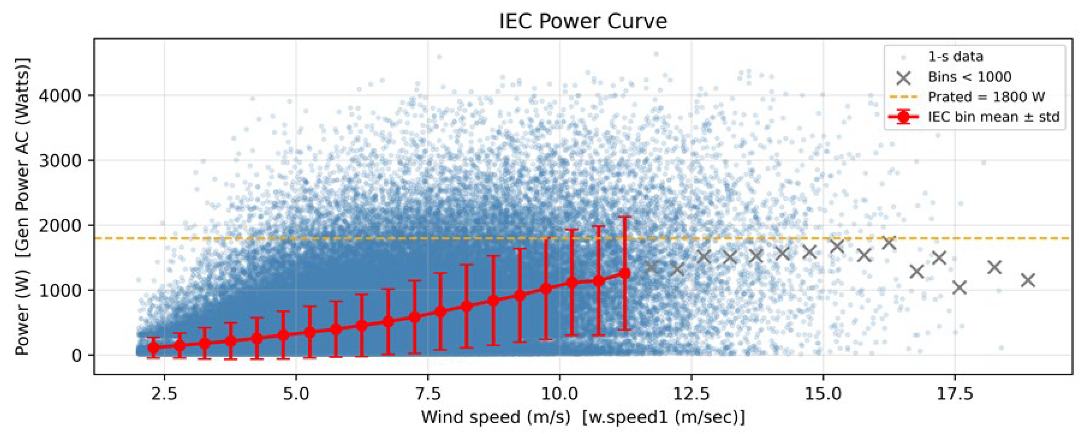
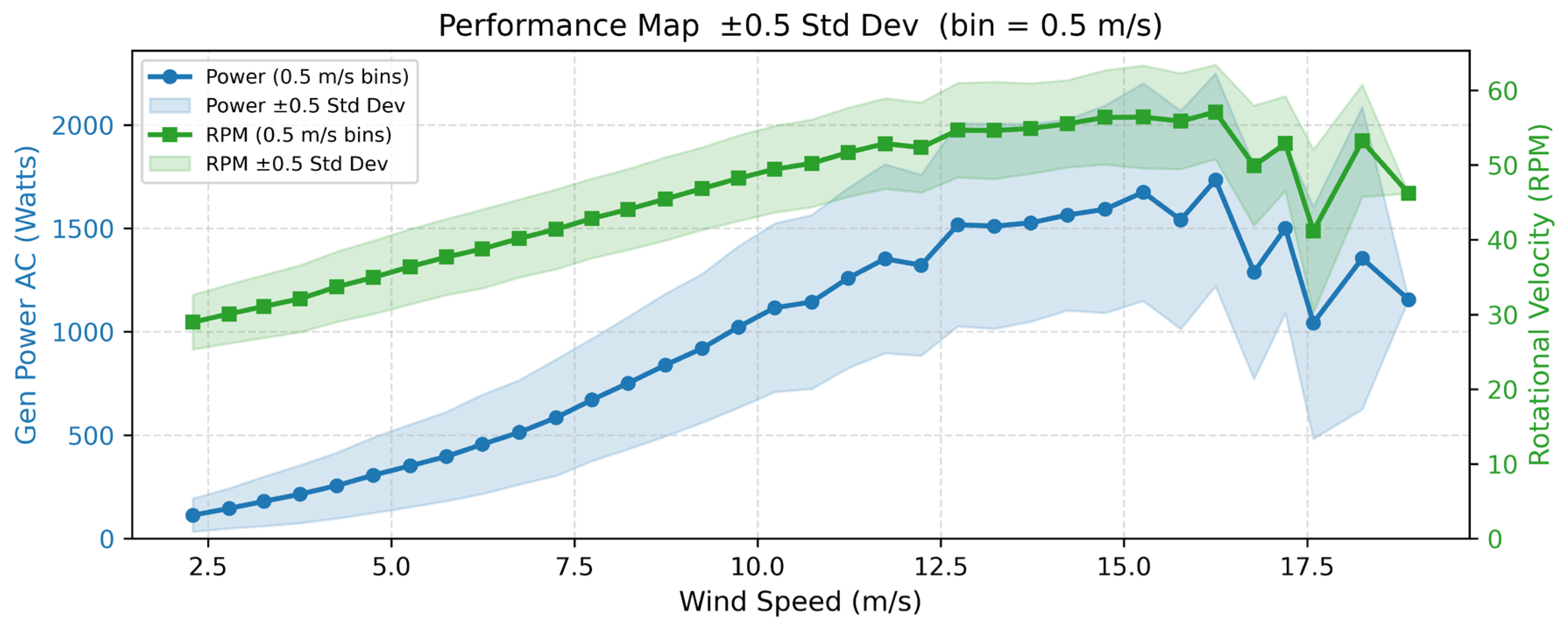
In Figure 8, a 1000-sample-minimum threshold of 1 s data is utilised for populating the bin averages. Valid bins (solid bars) extend from 2 m/s to 11.5 m/s, meaning the measurement campaign captured thousands of seconds at each of these wind speeds, a statistically robust dataset for that range. Beyond 12 m/s, all bins fall below 1000 samples (hatched bars), indicating that high-wind events are rare at this site. This is expected for a near-coastal Cretan location and is consistent with a Rayleigh mean well below 10 m/s. For a formal IEC 61400-12-1 assessment, one would need to accumulate at least 30 min (1800 s at 1 Hz) per 0.5 m/s bin across the full operating range, so the high-wind bins would need more measurement time before being reportable. The bin-averaged power curve rises monotonically from ~120 W at 2.5 m/s to a peak of roughly 1500–1600 W at 14–15 m/s. Here, cut-in is effectively set at approximately 2 m/s. The power filter minimum of 15 W already excludes noise, so anything appearing in the chart represents genuine generation. This is consistent with a high-solidity multi-sail rotor which starts turning at low wind speeds. The curve never reaches P_rated = 1800 W within the valid-bin range. Given that even the sparse high-wind bins peak around 1600–1700 W, rated power may be achievable only under brief periods of time. The scatter is extremely wide. The standard deviation at any given bin often equals or exceeds the mean (visible especially in Figure 9, where the blue cloud extends from near 0 W to 4000+ W at mid-range winds). This is partly instrumental (1 s data resolves every turbulent fluctuation, unlike 10 min averaging), but also reflects the aerodynamic character of the Cretan sail-rotor, where cloth sails with variable camber respond dynamically to each gust, creating far more instantaneous power variability than a rigid-blade turbine of similar size.

As seen in Figure 10, at V = 7 m/s with approx. 45 RPM, the tip speed ratio is, TSR = ω·R/V = (45 × 2π/60) × 2.75/7.0 ≈ 1.85. This is a very low TSR. Modern 3-blade HAWTs optimise around TSR 6–9 where Cp can reach 0.45–0.50. The Lasithi-type sail-rotor operates at TSR < 2 by design. Its many fabric sails create high torque at low speed, not high C_p. The Betz limit of 0.593 is far from reached, but this is entirely expected and physically consistent with the machine’s purpose and geometry. Also in Figure 10, the RPM curve is the most informative channel for understanding rotor aerodynamics. Below 10 m/s, RPM rises almost linearly with wind speed from ~30 RPM to ~55 RPM. This linear region indicates the rotor is operating in a torque-limited, nearly free-running regime, with the electrical load (and its braking torque) being relatively small compared to available aerodynamic torque, so the rotor accelerates with the wind. Above 10–12 m/s, RPM stabilises at ~55–58 RPM despite the wind continuing to increase. This is the aerodynamic stall/self-regulation region of the sail-rotor generator. The cloth sails passively deform and partially feather under increasing centrifugal and aerodynamic load, preventing runaway. This is the primary overspeed protection mechanism of the traditional design, in lieu of active pitch or furling. The stabilisation is clean and consistent—the tight RPM bands (narrow green shading) confirm this is a repeatable, physically stable regime, not measurement noise. Above ~16 m/s, both RPM and power drop. This is a combination of genuine furling at very high winds, with the cloth sails collapsing or reefing. The RPM standard deviation is dramatically smaller than the power standard deviation throughout. This tells us that the rotor inertia acts as a mechanical low-pass filter, with rapid wind gusts changing instantaneous power (proportional to V³) far more than they change RPM. For load calculations, this is important since the generator and structural components see a relatively smooth rotational speed but highly variable torque.

In Figure 8 and Figure 9, the transition from solid to hatched bars occurs abruptly at ~12 m/s, with the IEC scatter plot showing the high-wind “×” markers sitting below the P_rated line. Here, the aerodynamic stall regulation is evident, with power genuinely declining or saturating as the sails stall, consistent with the RPM stable region. Also, survivorship bias in the dataset is evident; when the operating system partially furls or stops the machine at high winds, the recorded high-wind data represents only brief, non-steady episodes.

It should be noted here that the power values reported in the field measurement power curve represent net electrical output measured at the inverter terminals, whereas CFD-predicted power is computed as aerodynamic shaft power P = Q ω, with no account taken of mechanical friction, generator losses, or inverter conversion efficiency. The observed agreement of 8–12% between CFD and field measurements across the 2–13 m/s attached-flow envelope, therefore, incorporates these conversion losses and should not be interpreted as the sole measure of CFD modelling accuracy.

5.2. Aerodynamic and Operational Analysis of the Sail-Rotor Based on the Computational Results

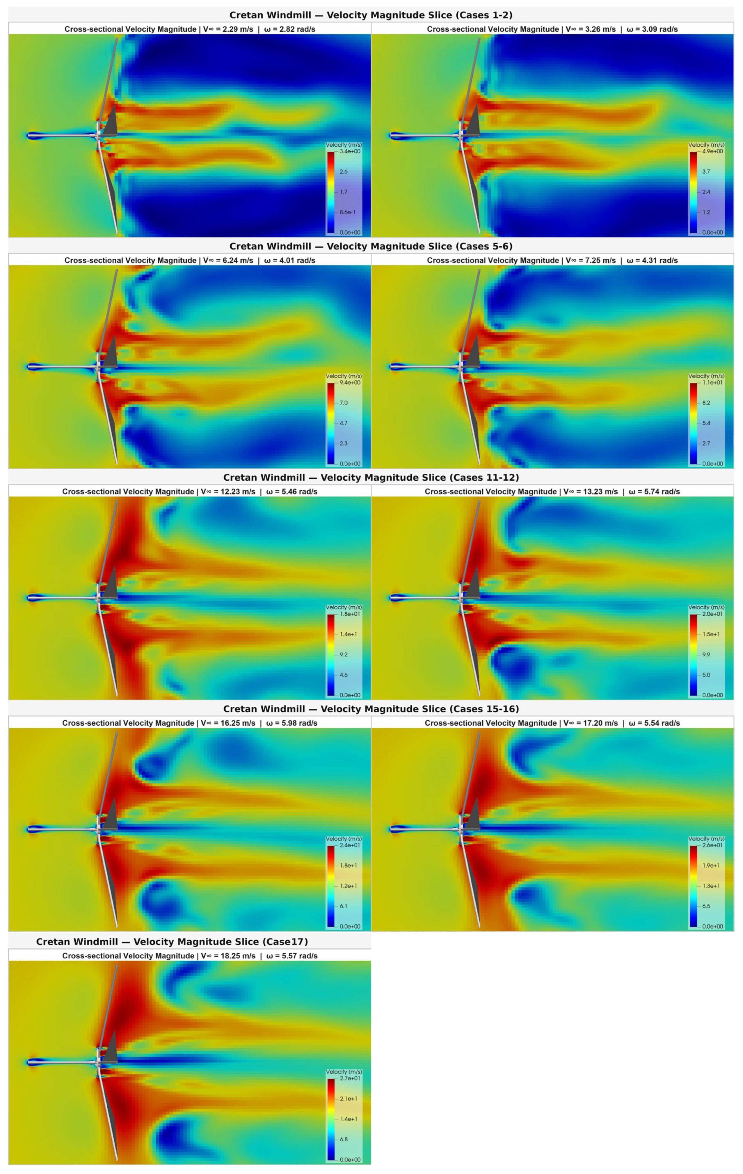
The simulations produced detailed information on flow trajectories, power generation, and the impact of boundary condition treatment. By examining the flow behaviour in Figure 11 and Figure 12 and taking into account the aerodynamic parameters in Table 7, three distinct aerodynamic regimes are immediately apparent. A high-TSR regime with λ > 2 (cases 1–3), a mid-TSR working range with λ ≈ 1.0–1.8 (cases 4–15), and a deep-stall/sail-furling regime with λ < 0.9 (cases 16–17).

Figure 11 shows the cross-sectional plots of the velocity magnitude (in m/s) for cases 1, 2, 5, 6, 11, 12 and 17. Across all cases, the upstream region shows a progressively expanding high-velocity (red/orange) zone as V∞ increases. This is the upstream induction effect, where the rotor disc acts as a partial actuator that decelerates the approaching stream, displacing mass flow radially outward and creating an annular speed-up band around the disc edge. In cases 1–2, the upstream field is nearly uniform green-blue, consistent with minimal rotor loading at low wind speed and relatively high TSR. The rotor is rotating with low torque and barely extracting momentum from the oncoming flow. In cases 11–12, the upstream red lobe is substantial and clearly asymmetric between the upper and lower half-planes. This asymmetry reflects the advancing/retreating blade effect inherent in the sliding-mesh formulation. The blade moving into the wind (advancing side, upper half in these plots) sweeps a higher relative velocity than the retreating side, generating stronger blockage on that half. The effect becomes more pronounced by case 11. In case 17, the upstream high-velocity region dominates nearly the entire left half of the domain. This shows that the rotor disc presents a high-resistance obstacle to the flow, which is consistent with the stalled sails acting as bluff bodies rather than lifting surfaces.

Let us consider now the near rotor flow behaviour regarding rotor loading and flow separation. In cases 1–4, where λ ranges between 1.96 and 3.39, the blade surfaces show no detectable separated flow. The velocity gradients across the chord are smooth, and the wake shed from each blade is thin and attached. This is a low-load operation—the angle of attack seen by each sail section is small because the high TSR means the relative wind vector is nearly tangential. In cases 5–8, where λ becomes 1.46 to 1.77, a visible, narrow, low-velocity blue filament extends downstream along the rotor axis, indicating a well-established axisymmetric hub wake. Behind each blade passage, discrete orange-to-green wake sheets are visible, showing blade-bound shedding vorticity. In cases 11–12 (λ = 1.19–1.22), the transition to moderate stall begins. In case 11, the near-wake immediately behind the rotor begins to show patchy blue regions on the leeward side of the lower blade, indicating leading-edge separation. By case 12 (V∞ = 13.23 m/s, λ = 1.19), a large, coherent dark-blue recirculation pocket appears below the hub and on the suction side of the lower blade. This is aerodynamic stall, with the boundary layer separated from the leeward face, and a low-pressure, near-zero-velocity recirculation zone has formed. In case 17 (λ = 0.84) the stall region extends to both blades. Two distinct dark-blue separated-flow zones now flank the hub symmetrically (upper and lower), and the near-wake contains large-scale vortical structures. The rotor is operating in deep stall across most of the sail span.

In order to fully describe the sail-rotor generator’s aerodynamic behaviour, it is important to evaluate the evolution of the wake structure throughout the different flow conditions. For cases 1 to 6, the downstream wake is a single elongated, well-defined velocity-deficit tube centred on the rotor axis. Its half-width expands slowly with downstream distance, and the velocity recovers gradually from the rotor-induced deficit back toward the freestream magnitude. The streamwise structure is smooth, indicating that blade-shed vorticity is organised in helical tip-vortex structures too tightly wound to resolve individually on this cross-sectional plane.

In cases 7 to 12, a transitional wake appears. The wake gains lateral width rapidly, and a tip-vortex distribution becomes visible as alternating high/low velocity patches flanking the wake boundary. For cases 13 to 17, a stalled wake is evident. The wake no longer resembles a slender momentum-deficit tube. Instead, it displays large-scale periodic shedding structures with broad alternating blue (slow) and yellow-green (faster) regions, characteristic of bluff-body vortex shedding from a heavily stalled rotor. The deficit extends across nearly the full domain width, and the near-wake recirculation zones merge with the far-wake structure. By case 17, the downstream domain contains two clearly distinct low-velocity regions symmetrically above and below the axis, which are the footprints of counter-rotating streamwise vortex pairs trailing from the stalled blade tips.

The colour bar maximum scales intentionally with the wind speed for a clearer view of the flow domain. The absolute peak velocity in each plot is consistently 1.45–1.55 × V∞. The minimum velocity (dark blue, near-zero m/s) is always co-located with (i) the hub centre, (ii) the blade trailing edge at peak-load conditions, and (iii) the separated-flow recirculation pockets in stalled cases. The most physically significant feature of the entire dataset is the reversal in ω between cases 15 and 16, where ω decreases from 5.98 to 5.54 rad/s even though V∞ increases from 16.25 to 17.20 m/s, and remains similarly decreased (5.57 rad/s) at case 17. This behaviour is characteristic of a deep-stall, low-TSR flow regime. Cases 16–17 show a mildly less severe near-rotor separation pattern compared to case 15, despite the higher V∞.

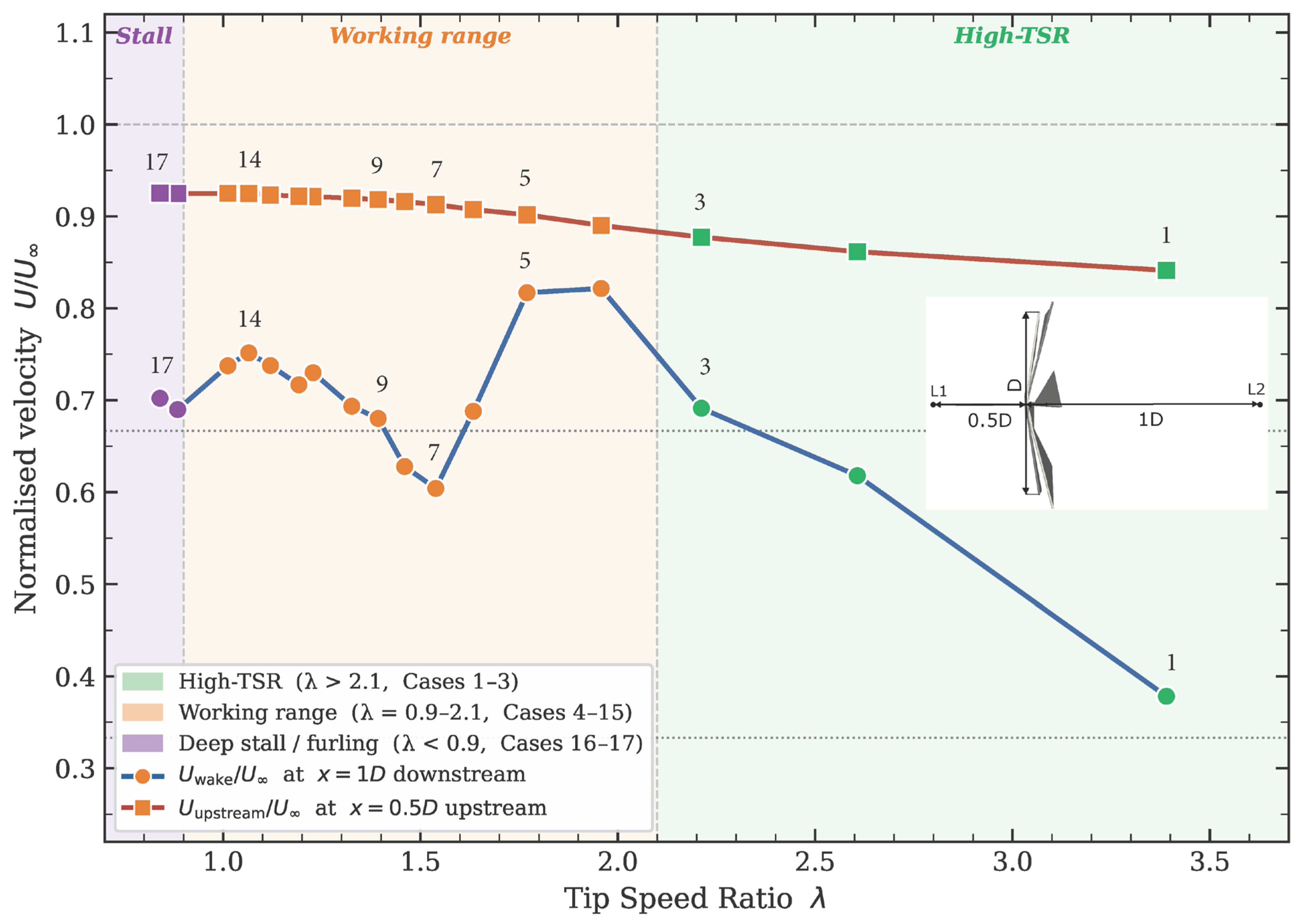
Figure 12 presents the two complementary probe measurements extracted from the CFD sweep as normalised ratios against tip speed ratio λ for all 17 operating points, revealing the full aerodynamic envelope of the Cretan windmill from cut-in through deep stall. The upstream induction curve (U_upstream/U∞, L1 probe at x = 0.5D upstream) decreases monotonically from 0.925 at the lowest TSR values (cases 16–17, λ < 0.9) to 0.841 at Case 1 (λ = 3.39). This implies that, at a distance of only 0.5D upstream of the rotor plane, the axial induction factor a has not yet fully developed, and the velocity field is dominated by the local pressure gradient of the approaching disc rather than the far-field momentum deficit. The gentle but consistent downward trend with increasing λ confirms that higher tip speed ratios impose a progressively stronger upstream blockage, consistent with the expanding upstream high-velocity lobe visible in the corresponding Figure 11 contours as λ increases. The wake centreline curve (U_wake/U∞, L2 probe at x = 1D downstream) displays a diverse, non-monotonic behaviour that encodes the full performance envelope. Starting from case 1 (λ = 3.39), where U_wake/U∞ = 0.378, the ratio rises steeply through the high-TSR regime to a pronounced double peak at cases 4–5 (λ ≈ 1.77–1.96, U_wake/U∞ ≈ 0.82), which corresponds to the maximum energy extraction by the windmill. This peak is followed by a local trough at cases 6–7 (λ ≈ 1.54–1.63, Uwake/U∞ ≈ 0.60–0.63), which reflects the onset of organised tip-vortex shedding and blade-passage asymmetry first visible in Figure 11 at those cases. The wake begins to lose its axial symmetry, and the centreline probe samples are more disrupted, indicating a locally lower-velocity region. A partial recovery occurs through cases 8–15 as the rotor progressively stalls and the wake transitions from a tip-vortex-dominated structure to a broader bluff-body wake, which unexpectedly carries more momentum at the centreline than the structured vortex-shedding regime. In the two stall cases (16–17, λ < 0.9), which sit at U_wake/U∞ ≈ 0.69–0.70, the wake centreline velocity is mildly recovered. This reflects the aerodynamic response of a rigid high-solidity rotor operating at very low TSR. Throughout the working range, the wake curve remains between the two Betz reference lines (1/3 < U_wake/U∞ < 2/3), which is precisely the theoretical condition for net positive power extraction from an actuator disc, independently validating that the CFD solutions in this regime are physically consistent with momentum theory.

In multi-blade arrangements, hub vortices and strong wake deficits would increase wake interactions, reduce downstream power recovery, and raise unsteady load fluctuations, similar to those widely reported in the relevant literature [30,35,36].

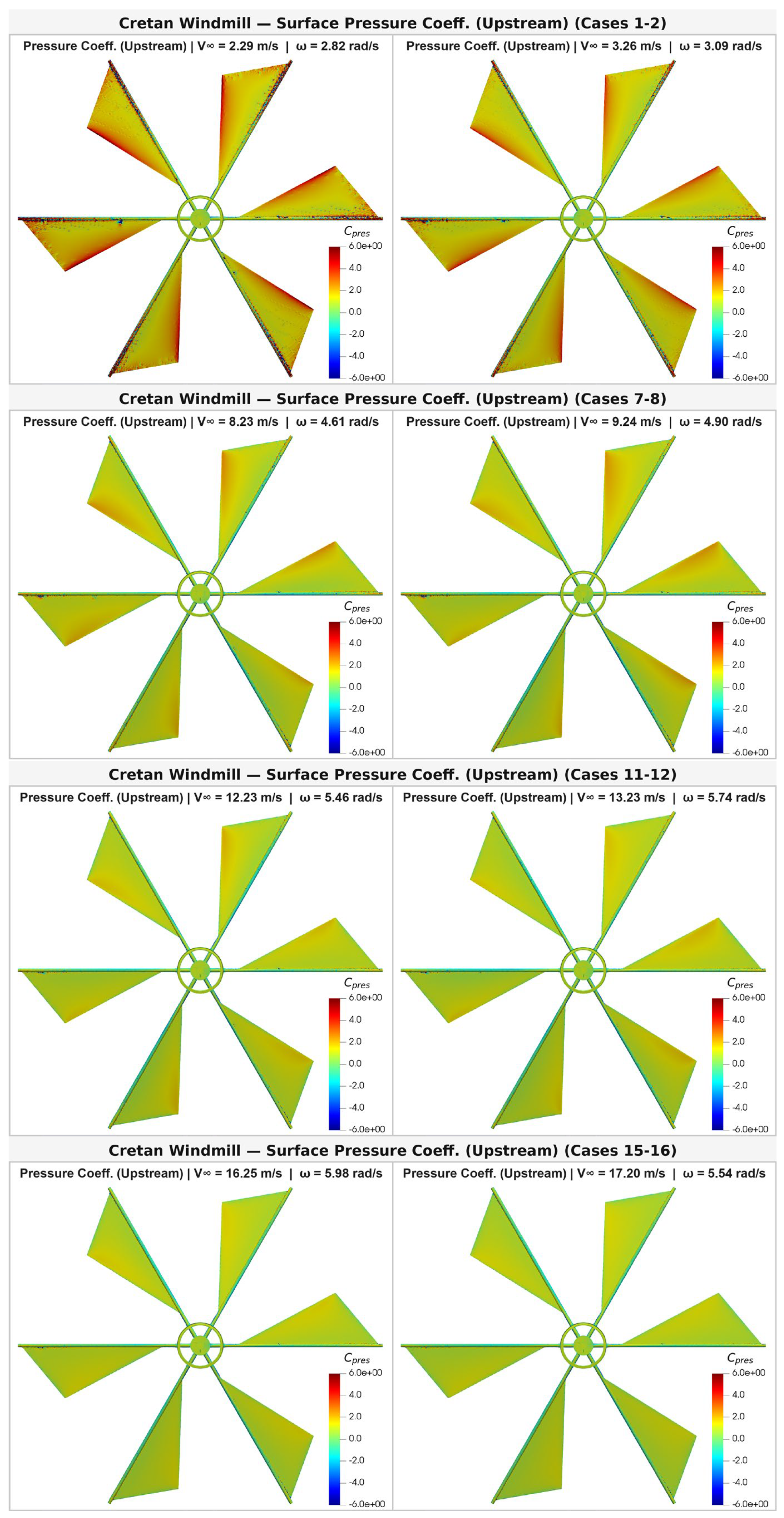
The upstream surface pressure coefficient (C_pres) in Figure 13 and Figure 14 decreases monotonically in magnitude from the saturated red of cases 1 to 3 to the uniform green of cases 16 to 17. C_pres is normalised by the freestream dynamic pressure q∞ = ½ρ$V_{\mathrm{\infty }}^2$, which itself grows as $V_{\mathrm{\infty }}^2$ across the sweep. The distinctive red saturation of cases 1 and 2, therefore, does not indicate the highest structural loads in the campaign, quite the opposite. The actual aerodynamic force per unit area is maximised at cases 15 to 17, where the subdued green palette masks absolute pressures that are tens of times larger than those at cut-in. With that established, the C_pres distributions reveal three physically distinct aerodynamic regimes that map precisely onto the wake topologies described in the velocity analysis of Figure 11 and Figure 12. At high TSR (cases 1–3, λ = 2.2–3.4), the windward face is nearly uniformly loaded across the full chord and span, with no discernible chord-wise gradient. This pressure uniformity is characteristic of drag-dominated, near-flat-plate loading, where the blade tip speed greatly exceeds V∞, the effective angle of attack in the rotating frame is very large, and the sail stagnates the incoming flow almost uniformly across its surface rather than generating an organised leading-edge suction peak. As TSR decreases through cases 4 to 9 (λ = 1.4–2.0), two systematic gradients emerge and sharpen. First, a chord-wise gradient develops, where C_pres is highest at the leading (outer radial) edge and decays toward the trailing (inner) edge. This is the surface pressure signature of an attached boundary layer with a defined stagnation point and downstream pressure recovery. Its appearance marks the transition from purely drag-driven to mixed lift-drag operation and is directly responsible for the organised tip-vortex shedding and coherent hub-wake streak that first appear in the velocity slices at cases 5 and 6. Second, a strong radial gradient establishes itself with higher C_pres at the tip and lower values at the root, reflecting the ωr-dependent dynamic pressure seen by each blade section and explaining why the tip region is the primary site of vortex shedding and wake entrainment in the velocity field.

The stall progression from cases 11 to 15 is clearly encoded in the upstream C_pres. The chord-wise gradient first collapses inboard, with the inner sail sections losing their leading-edge pressure concentration while the outer 30 to 40% of the span retains it. By case 15, the distribution is nearly flat and uniform across the entire sail (green, C_pres ≈ 0.3–1.5). Crucially, the C_pres pattern changes very little between cases 13, 14, and 15 despite V∞ increasing by over 2 m/s, because of the fact that the rotor has entered a regime where the blade loading is governed entirely by the stalled-plate pressure coefficient and is insensitive to further changes in either V∞ or ω. This is the pressure-field counterpart of the ω saturation and bluff-body wake confirmed in the velocity plots for the same cases. Finally, cases 16 to 17 show a C_pres level that is marginally lower than cases 14 to 15, despite the highest wind speeds in the campaign. This drop in Cpres and ω in cases 16–17 is due to the aerodynamic loading change, which is, in turn, associated with the lower TSR.

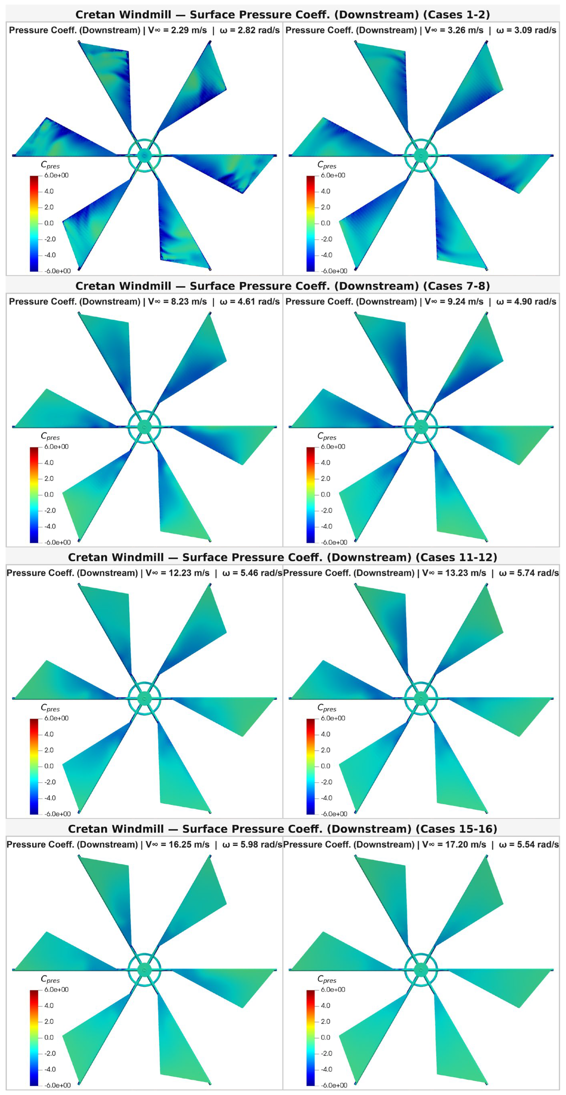
The downstream surface in Figure 14 is the suction side of the sail and carries negative C_pres throughout the entire operating range, as expected for a surface from which the flow accelerates away rather than impinging upon. The net aerodynamic force driving rotor rotation is proportional to ΔC_pres = C_{pres,upstream} − C_{pres,downstream} across the two faces. The most immediate and physically important observation is that the downstream face shows the inverse of every trend identified on the upstream face, i.e., where upstream C_pres increases with decreasing λ (due to the normalisation effect discussed previously), the downstream suction magnitude peaks in the mid-TSR working range and diminishes toward both extremes of the sweep, providing a direct surface pressure record of the rotor’s aerodynamic efficiency envelope.

At high TSR (cases 1–3, λ = 2.2–3.4), the downstream surface presents an inherently unsteady and low-Reynolds-number flow regime. The absolute pressure difference across each sail is very small in physical terms, and the sail-rotor generator is barely loaded.

The transition to a physically interpretable, well-structured suction distribution begins at cases 4 to 6 (λ = 1.6–2.0) and sharpens progressively through cases 7 to 9 (λ = 1.4–1.5), which represent the most aerodynamically active region of the entire sweep. By case 7, the downstream face shows a sharply defined, deep-blue suction concentration at the leading edge and outer tip region, transitioning to teal toward the trailing edge and root. This is the classical distribution of an attached turbulent boundary layer with a strong leading-edge suction peak. Here, the flow accelerates tightly around the outer radial edge of the triangular sail, creating a local low-pressure zone that is the primary lift-generating mechanism. The chord-wise gradient is steep near the leading edge, relaxes toward the trailing edge, mirrors and directly complements the positive chord-wise gradient on the upstream surface, confirming that the sail is operating as an aerodynamic surface rather than a simple drag device. The radial gradient, with maximum suction at the tip and diminishing values toward the root, is consistent with the higher relative velocity at large R and is the surface pressure source for the well-organised tip vortex shedding and deepening wake-deficit structures identified in the corresponding velocity contours. The azimuthal blade-to-blade variation in suction magnitude, where blades whose leeward face is more directly shielded from the downstream wake show reduced C_pres magnitude, mirrors the advancing/retreating blade asymmetry already observed on both the upstream face and in the velocity field.

From cases 10–12 (λ = 1.2–1.33) onward, the downstream suction distribution progressively deteriorates in a spatially coherent manner that constitutes the clearest surface pressure record of stall progression in the dataset. The leading-edge suction peak first weakens and retreats inboard—surviving only at the outer 30–40% of span by case 11, before collapsing entirely across the full chord by cases 13–15. This inboard-to-outboard stall propagation is perfectly consistent with the root-first separation identified from the upstream C_pres analysis and with the large leeward recirculation pockets visible in the velocity slices for cases 11–12. Once the boundary layer separates at the leading edge of the inner blade sections, the flow can no longer accelerate around the surface, the suction peak vanishes, and the downstream face C_pres rises from negative values toward zero. By cases 13–15 (λ = 1.0–1.1), the leeward face shows a nearly uniform teal-green distribution (C_pres ≈ −1 to −2) with no chord-wise gradient, consistent with a fully separated, bluff-body leeward flow field. The convergence of upstream and downstream C_pres toward similarly low absolute magnitudes means ΔC_pres is small, the net aerodynamic torque per unit area is minimal, and the rotor is extracting almost no energy with the surface pressure counterpart of the bluff-body wake, and ω saturation is seen in the velocity plots for the same cases. In cases 16–17, the downstream face becomes even more uniformly teal-to-cyan, and the suction values are the mildest in the sweep. The reduced effective area means both a smaller stagnation face (upstream) and a smaller suction face (downstream), with ΔC_pres remaining similarly depressed, which is a consequence of deep aerodynamic stall at low TSR.

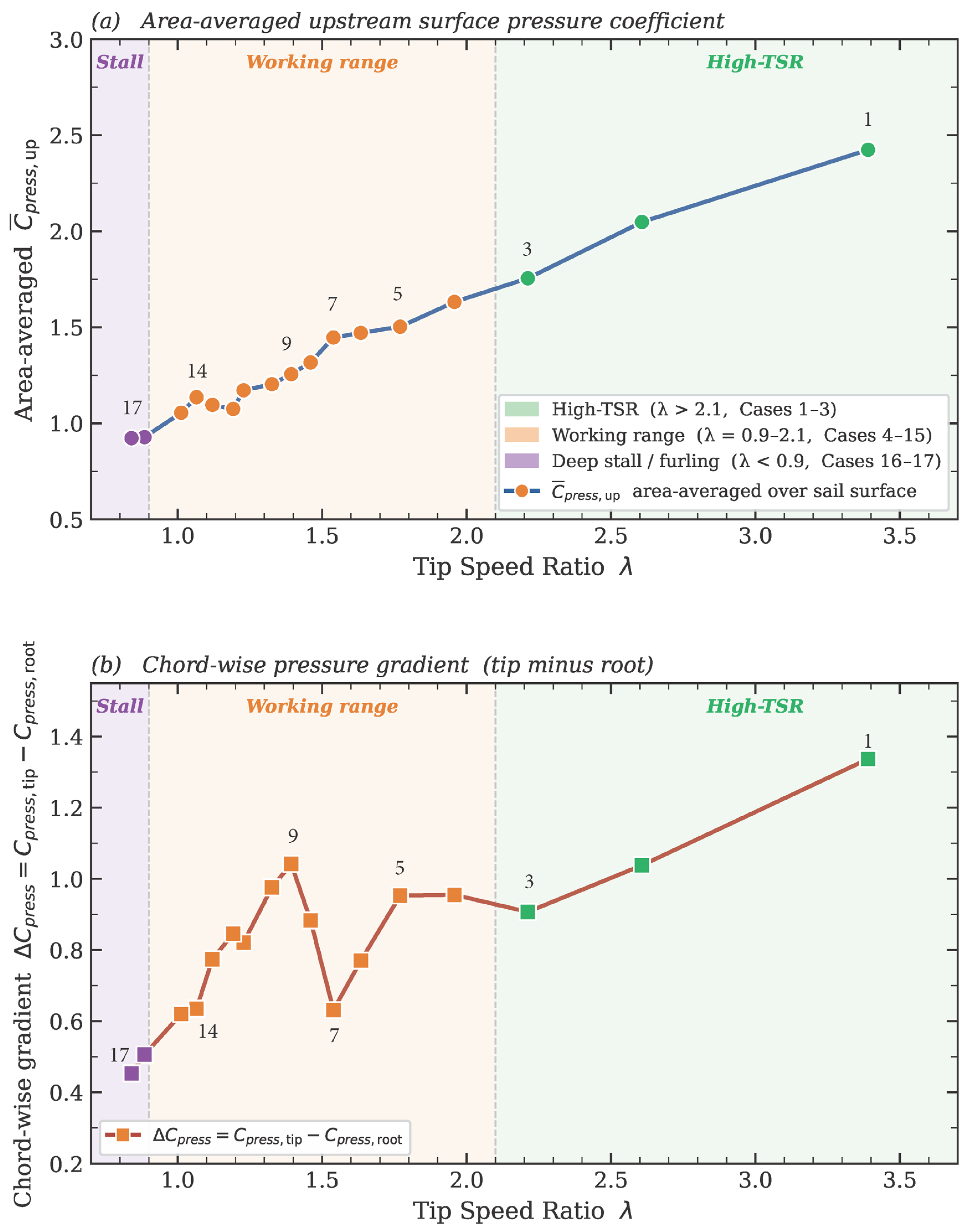
Figure 15 quantifies the two complementary aerodynamic signatures of the upstream surface pressure field, which are already visible qualitatively in Figure 13. The area-averaged upstream, C_pres,up (Figure 15a), changes monotonically with increasing tip speed ratio λ, from ≈0.92 in the deep-stall regime (cases 16–17, λ < 0.9) through the working range, up to a maximum of ≈2.4 at case 1 (λ = 3.39). The chord-wise gradient, ΔCpres = Cpres,tip − Cpres,root (Figure 15b), is different. From cases 1 through 5 (λ = 1.77–3.39) the gradient drops from 1.34 to 0.95, thus reflecting the progressive reduction in the centrifugal dynamic pressure advantage at the tip as the relative velocity between tip and root narrows with decreasing TSR. The trough in case 7 (λ = 1.54, ΔCpres ≈ 0.63) coincides with the onset of the blade-to-blade advancing/retreating asymmetry, where the retreating blade sees a lower relative velocity, depressing its tip pressure and temporarily equalising the radial distribution. The sharp recovery to the peak gradient at case 9 (λ = 1.39, ΔCpres ≈ 1.04) marks the aerodynamic transition point, since this is the last operating condition at which the tip region retains a clearly elevated stagnation concentration while the inner sail sections begin to show signs of separation. Beyond this peak, the gradient declines steadily through cases 10–15 as stall propagates radially outward, and the tip progressively loses its pressure advantage, reaching λ ≈ 1.01–1.12, where the surface pressure plots show a nearly uniform distribution across the entire sail span. cases 16–17 display the minimum gradient (ΔCpres ≈ 0.45–0.51), confirming deep-stall sail-rotor operation.

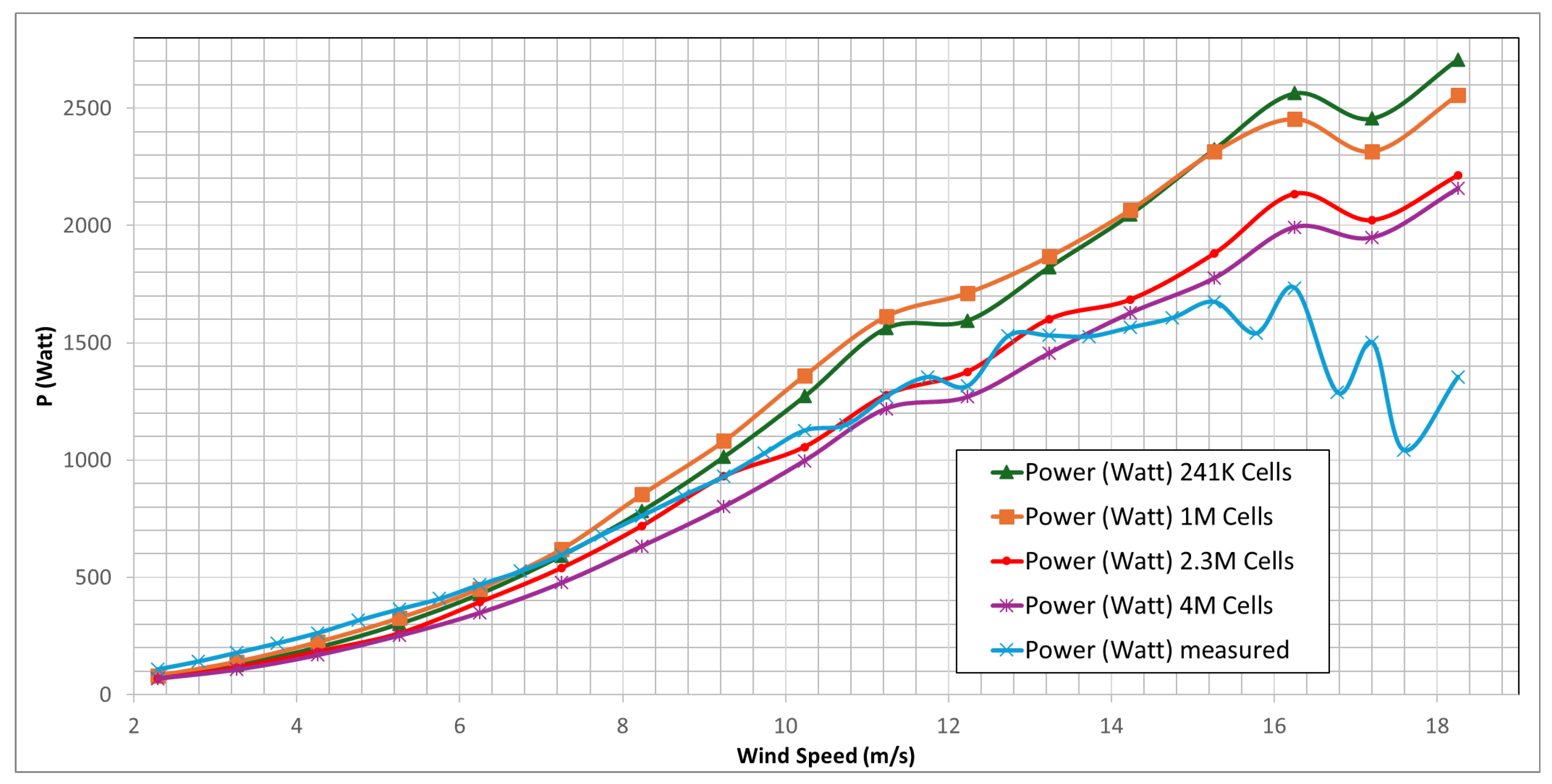
Figure 16 compares the power curve results across the four CFD grid types (Table 3) and the experimental measurements of the sail-rotor generator. The CFD results exhibit well-behaved monotonic convergence throughout the operating range, with the predicted power decreasing systematically as the mesh is refined from 241 K to 1 M to 2.3 M to 4 M cells, a pattern consistent with the progressive reduction in numerical diffusion as grid resolution improves. On coarser meshes, insufficient resolution of the sail boundary layers and tip-vortex cores introduces artificial numerical viscosity that effectively over-smooths the shear layers, suppresses resolved separation, and inflates the computed torque. At 241 K cells, the overprediction relative to the finest mesh reaches 15–25% across the full operating range, confirming this mesh is clearly inadequate. The 1 M-cell mesh reduces but does not eliminate this bias, remaining 10–15% above the 4 M prediction at wind speeds above 10 m/s. The most important convergence result is the close agreement between the 2.3 M and 4 M solutions below approximately 13 m/s, where the two curves are nearly indistinguishable. This near-coincidence indicates the solution has entered the asymptotic convergence zone and that the 2.3 M mesh is approaching grid independence for the attached-flow portion of the operating envelope. In the low-to-mid wind speed range (2–10 m/s), all four CFD meshes agree reasonably with the measured power curve. The 4 M and 2.3 M predictions bound the measured data from above, with discrepancies generally within 8–12%, which is acceptable given that the measurements represent electrical output at the grid connection (inclusive of inverter and generator losses not accounted for in the CFD torque integral) while the simulations compute aerodynamic shaft power directly as P = Qω. The slight inflexion visible in several CFD curves near 8–9 m/s corresponds to the onset of inboard stall, as noted in the previous pressure coefficient analyses, and marks the boundary between the attached-flow and progressive-stall regimes in the simulation. The measured curve passes through this region smoothly, suggesting that the real machine’s flexible sails naturally delay or spread the stall onset through aeroelastic washout, a behaviour the rigid-geometry CFD cannot currently reproduce.

Above approximately 13 m/s, all four CFD meshes continue to predict monotonically increasing power, reaching 2100–2700 W at 18 m/s, depending on refinement level. The measured curve, by contrast, peaks near 1720 W at 16 m/s, then drops sharply. This non-monotonic, oscillatory high-wind behaviour is the power curve expression of the traditional Cretan sail-furling mechanism. Above the onset wind speed, the sail panels’ geometry alters, capping the aerodynamic torque. Because all CFD cases in the current attempt use fixed, fully deployed sail geometry, this mechanism is entirely absent from the simulations. The discrepancy above 13 m/s, therefore, constitutes the primary quantitative motivation for the FSI extension of this work, with a coupled aeroelastic simulation that allows the sail to deform, reef, and spill load at high incidence angles to recover the measured high-wind power reduction. The present rigid-body CFD sweep establishes the upper bound of aerodynamic performance that would be achieved with a perfectly stiff, fully deployed sail. The difference between this bound and the measured curve at each wind speed is an approximate indication of the combined effect of sail aeroelasticity, which includes but is not limited to load-shedding through flexible deformation, a behaviour that the future FSI extension is specifically designed to isolate and quantify.

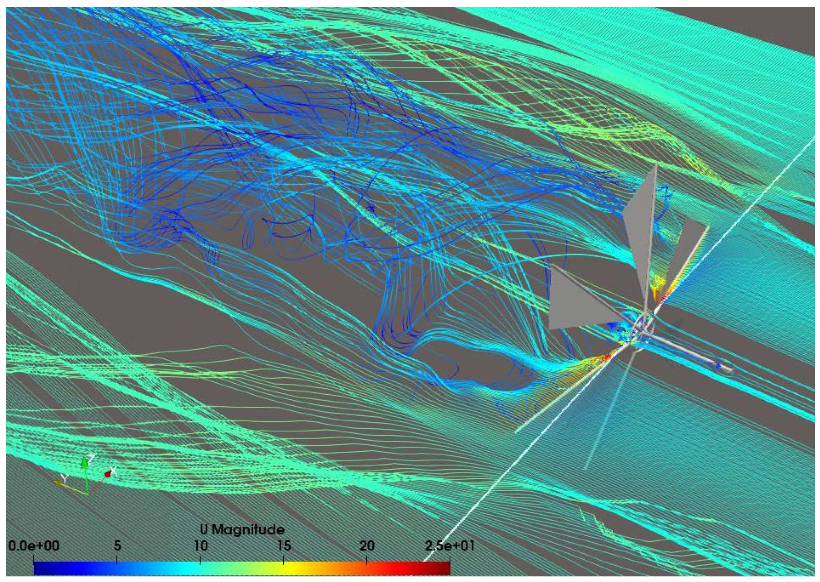
In Figure 17, it is very interesting to notice the helical tip-vortex system shedding continuously from each blade tip as it sweeps through the rotor plane (case 11, V∞ = 12.2318 m/s, ω = 5.46009 rad/s, λ = 1.2276). Each blade generates a bound circulation that must, by Helmholtz’s theorem, terminate as a free vortex filament at the tip and at the root. The tip filaments roll up into concentrated helical vortex tubes that convect downstream and radially outward, forming the characteristic corkscrew structure of a rotating-blade wake. In this visualisation, the individual helical turns from successive blade passages have interacted and begun to merge through vortex pairing—a well-documented instability of wind turbine helical wakes in which adjacent vortex filaments of the same sign spring and coalesce into larger, lower-frequency vortical structures. The result is the visually chaotic but physically organised tangle of swirling streamlines seen in the near-to-mid wake: what appears disordered is actually the superposition of several partially merged helical vortex tubes, each retaining a coherent low-velocity core (hence the persistent deep blue), surrounded by entrained fluid being pulled into rotational motion. The swirl component visible in the wake streamlines is a direct measure of angular momentum imparted to the fluid by the rotor. Τhe reaction torque driving the rotor is equal and opposite to the torque exerted on the fluid, which manifests as this circumferential velocity component that persists far downstream. The streamlines that enter the rotor disc region exit as helical trajectories with both a reduced axial component, i.e., the momentum deficit corresponding to energy extraction and a newly acquired tangential component in the rotor’s direction of rotation. This swirl energy embedded in the wake is aerodynamically lost, since it cannot be recovered by the rotor and represents the rotational kinetic energy irreversibly deposited into the fluid, which, in actuator disc theory, contributes to the deviation of real turbine performance below the Betz limit. The persistence of strong swirl well into the far wake is characteristic of low-TSR machines such as this Cretan sail-rotor. At higher TSR, the swirl-to-axial velocity ratio is lower and wake rotation recovers faster, but at the TSR values of this sweep (λ = 1.2276), the tangential induction factor a′ is large and swirl losses are substantial. The high-velocity yellow-orange streamlines concentrated immediately around the blade tips and surfaces represent the superposition of freestream velocity and the local tangential blade velocity ωr, which at the tip reaches 15–16 m/s for this high-wind case. Streamlines originating at the hub centre converge toward the axis from both sides of the rotor plane, tracing the hub vortex.

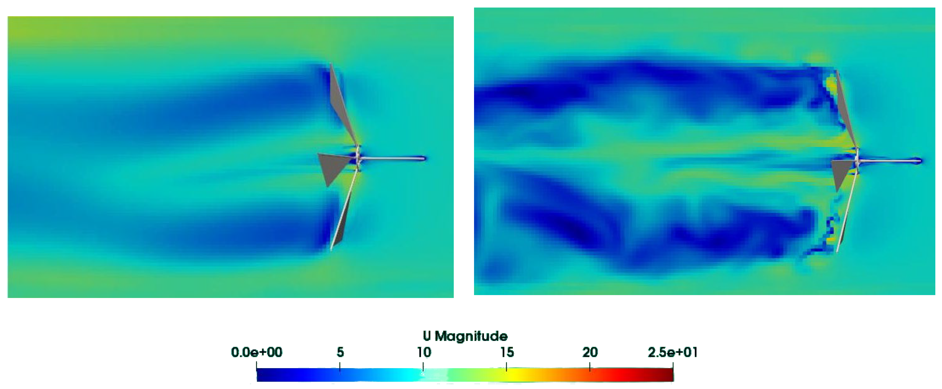
One final thing to notice in Figure 18 is the difference between the results of the classic k–ε and the k–ω SST turbulence models in terms of the representation of the separated wake flow. At case 11 (λ = 1.23), the k–ε model predicts a narrow, well-organised wake with no discernible blade-surface separation, while the k–ω SST solution produces a dramatically wider wake, multiple distinct low-velocity recirculation zones on the leeward blade surfaces, and sharp, internally structured shear layers, a topology entirely consistent with separated-flow pattern, independently identified in the velocity slices in Figure 11 and C_pres analyses for this operating point in Figure 13 and Figure 14. The discrepancy is thoroughly discussed in Section 2.2 and the references therein. The k–ω SST solution is therefore adopted exclusively for the parametric sweep, and the contrast between the two panels provides direct visual justification for that choice.

6. Conclusions

A combined CFD and experimental characterisation of a full-scale six-sail Cretan windmill of the Lasithi type has been carried out, integrating a 17-case parametric OpenFOAM sweep with a field measurement campaign conducted in accordance with IEC 61400-12-1:2005(E). Grid independence is achieved at 2.3 million cells for the attached-flow operating range. The 2.3 M and 4 M meshes produce power predictions that differ by less than 3% below 13 m/s, while the 241 K and 1 M meshes overpredict aerodynamic shaft power by 15–25% and 10–15%, respectively, owing to insufficient resolution of blade boundary layers and tip-vortex cores. Τhe 2.3 M mesh is therefore identified as the minimum refinement level for design-point simulations.

Turbulence model selection is critical for this rotor class. The standard k–ε closure systematically suppresses blade-surface separation through unphysical eddy viscosity overprediction in adverse pressure gradient regions, yielding an artificially narrow wake and inflated torque estimates. The k–ω SST model correctly reproduces the large leeward recirculation pockets and broad wake structure, as independently verified in both the velocity field and surface pressure distributions, and is the appropriate closure for the separated-flow conditions encountered below λ ≈ 1.5.

Three aerodynamic regimes govern the rotor operation across the parametric sweep. At high TSR (λ > 2.1), the rotor operates in a drag-dominated, low-loading regime with nearly uniform upstream surface pressure and a diffuse wake. In the working range (λ ≈ 1.0–2.1), organised chord-wise and radial pressure gradients develop on both sail faces, confirming mixed lift–drag aerodynamic operation with peak loading near λ ≈ 1.4–1.5. The sail-rotor stalling initiates at the inner blade root sections and propagates outward as λ decreases. In the deep-stall regime (λ < 1.0), the boundary layer has separated across the full chord, the rotor presents a fully bluff-body wake, and angular velocity saturates at approximately 57 RPM.

In this work, passive overspeed self-regulation is field-validated. Above 13 m/s, the measured rotor speed stabilises at 55–58 RPM without any active control mechanism, and the angular velocity drops from 5.98 to 5.54 rad/s between cases 15 and 16 despite increasing wind speed. The field data confirm that this behaviour originates in the aeroelastic load-shedding of the flexible woven polyester sails, which progressively reduce effective disc solidity at high wind speeds. This mechanism is correctly identified in trend by the rigid-geometry CFD simulation, but it is overestimated in magnitude by 8–12% in shaft power. CFD–experiment agreement within this error magnitude across the 2–13 m/s operating range validates the adopted computational methodology for the attached-flow envelope. The residual discrepancy is attributable to mechanical and electrical losses not included in the aerodynamic shaft power computation and to the rigid-geometry assumption of the CFD model, which cannot reproduce the aeroelastic sail deformation governing performance above rated wind speed.

The primary limitation of this study is the rigid-sail assumption of the CFD model. All 17 simulations use fixed, fully deployed sail geometry and cannot reproduce the aeroelastic deformation, reefing, and load-shedding of the flexible woven polyester sails that govern rotor behaviour above rated wind speed. The gap between the rigid-geometry CFD upper bound and the measured power in the high-wind regime is consistent with a significant aeroelastic contribution but cannot be quantified without a coupled fluid–structure interaction model.

The results establish a validated computational and experimental baseline for the planned FSI extension of this work. Quantification of blade tip displacements, operational stress distributions, and the aeroelastic contribution to passive overspeed regulation are identified as the immediate next steps and will provide the first fully validated aeroelastic characterisation of this traditional rotor class.

References

1. Calvert, N.G. The characteristics of a sail mill. J. Wind Eng. Ind. Aerodyn. 1978, 3, 79–84. [Google Scholar] [CrossRef]
2. Demelis, N. The Restoration and Sustainable Development of the Traditional Aeolian Park of Lassithi Plateau, Crete (Greece). Past, Present, Future. Ph.D. Thesis, Universita degli Studi di Milano-Bicocca, Milan, Italy, 2017. [Google Scholar]
3. Fleming, P.D.; Probert, S.D. Design and performance of a small shrouded cretan windwheel. Appl. Energy 1982, 10, 121–139. [Google Scholar] [CrossRef]
4. Fleming, P.D.; Probert, S.D. Flexible sail wind-turbines: Review of pertinent theoretical analyses. Appl. Energy 1984, 18, 89–99. [Google Scholar] [CrossRef]
5. Ghosh, P.; Kamoji, M.A.; Date, A.W.; Prabhu, S.V. Experimental Investigations on Sail Type Wind-Turbines. Sage J. 2009, 33, 349–359. [Google Scholar] [CrossRef]
6. Kanaki, M.T.; Probert, S.D. Cretan windmills. Appl. Energy 1979, 5, 215–222. [Google Scholar] [CrossRef]
7. Calvert, N.G. Windpower in Eastern Crete. Trans. Newcom. Soc. 1971, 44, 137–144. [Google Scholar] [CrossRef]
8. Rossi, C.; Russo, F.; Savino, S. Windmills: Ancestors of the wind power generation. Front. Mech. Eng. 2017, 12, 389–396. [Google Scholar]
9. Skapoula, A.; Katsigianni, P.; Van den Broeck, P. Bridging the Gaps Between Past and Present for a Sustainable Future Energy Transition and the Case of the Lassithi Plateau. Master’s Thesis, KU Leuven, Faculteit Wetenschappen, Leuven, Belgium, 2024. [Google Scholar]
10. Condaxakis, C.; Ntintakis, I.; Kozyrakis, G.V.; Chrysoulakis, C.; Chatzakis, G.; Dakanali, E.; Papadakis, N.; Katsaprakakis, D. The Evolution of Windmill Design: From Lasithi Plateau Pumping Windmills to Electricity Production. Energies 2026, 19, 829. [Google Scholar] [CrossRef]
11. Mehmood, Z.; Wang, Z.; Zhang, X.; Shen, G. Aerodynamic Performance and Numerical Validation Study of a Scaled-Down and Full-Scale Wind Turbine Models. Energies 2024, 17, 5449. [Google Scholar] [CrossRef]
12. Rojas-Sola, J.I.; Bouza-Rodríguez, J.B.; Menéndez-Díaz, A. Technical and functional analysis of Spanish windmills: 3D modeling, computational-fluid-dynamics simulation and finite-element analysis. Energy Convers. Manag. 2016, 123, 130–139. [Google Scholar] [CrossRef]
13. OpenFoam. OpenFOAM v2412 User Guide; The OpenFOAM Foundation: London, UK, 2024. [Google Scholar]
14. Weller, H.G.; Tabor, G.; Jasak, H.; Fureby, C. A tensorial approach to computational continuum mechanics using object-oriented techniques. Comput. Phys. 1998, 12, 620–631. [Google Scholar] [CrossRef]
15. John, I.H.; Vaz, J.R.P.; Wood, D.H. Aerodynamic Performance and Blockage Investigation of a Cambered Multi-Bladed Windmill; IOP Publishing: Bristol, UK, 2020. [Google Scholar]
16. John, I.H.; Wood, D.H.; Vaz, J.R.P. Helical vortex theory and blade element analysis of multi-bladed windm ills. Wind Energy 2023, 26, 228–246. [Google Scholar]
17. Aized, T.; Sohail Rehman, S.M.; Kamran, S.; Kazim, A.H.; Ubaid ur Rehman, S. Design and analysis of wind pump for wind conditions in Pakistan. Adv. Mech. Eng. 2019, 11, 1687814019880405. [Google Scholar] [CrossRef]
18. Okura, S.S.; Ponte, M.C.A.; Palombella, F.O.; Almeida, J.R.F.; Dos Santos Matos, F.F. Evaluation of direct coupling between conventional windmills and rever se osmosis desalination systems at low wind speeds. Energy Convers. Manag. 2023, 295, 117654. [Google Scholar]
19. Pérez-Martín, E.; Herrero-Tejedor, T.R.; Gómez-Elvira-González, M.Á.; Rojas-Sola, J.I.; Conejo-Martín, M.Á. Graphic study and geovisualization of the old windmills of La Mancha (Spain). Appl. Geogr. 2011, 31, 941–949. [Google Scholar] [CrossRef]
20. Zayats, I.M. The historical aspect of windmills architectural forms transformation. Procedia Eng. 2015, 117, 685–695. [Google Scholar] [CrossRef][Green Version]
21. Castro-García, M.; Rojas-Sola, J.I.; Carranza-Cañadas, M.D.P. Technological characterization of Spanish Mediterranean windmills. DYNA 2013, 80, 22–30. [Google Scholar] [CrossRef]
22. Wu, X.; Lee, D. An electromagnetic energy harvesting device based on high efficiency w indmill structure for wireless forest fire monitoring application. Sens. Actuators A Phys. 2014, 219, 73–79. [Google Scholar]
23. Le-Huy, H.; Anderson, J. A microprocessor-controlled windmill simulator. In Energy Developments: New Forms, Renewables, Conservation; Pergamon: Oxford, UK, 1984. [Google Scholar]
24. Tortell, J.P. Reconversion of traditional water extraction windmills in mallorca to produce electrical power. Renew. Energy Power Qual. J. 2004, 2, 1. [Google Scholar]
25. Porté-Agel, F.; Bastankhah, M.; Shamsoddin, S. Wind-Turbine and Wind-Farm Flows: A Review. Bound. Layer Meteorol. 2020, 174, 1–59. [Google Scholar]
26. Menter, F. Two-equation eddy-viscosity turbulence models for engineering applications. AIAA J. 1994, 32, 1598–1605. [Google Scholar]
27. Wilcox, D.C. Turbulence Modeling for CFD, 3rd ed.; DCW Industries: La Canada, CA, USA, 2006. [Google Scholar]
28. Sørensen, N.N.; Michelsen, J.A.; Schreck, S. Navier–Stokes predictions of the NREL phase VI rotor in the NASA Ames 80 ft × 120 ft wind tunnel. Wind Energy 2002, 5, 151–169. [Google Scholar] [CrossRef]
29. Tachos, N.S.; Filios, A.E.; Margaris, D.P. A comparative numerical study of four turbulence models for the prediction of horizontal axis wind turbine flow. Proc. Inst. Mech. Eng. Part C 2010, 224, 1973–1979. [Google Scholar] [CrossRef]
30. Vermeer, L.J.; Sørensen, J.N.; Crespo, A. Wind turbine wake aerodynamics. Prog. Aerosp. Sci. 2003, 39, 467–510. [Google Scholar] [CrossRef]
31. Greenshields, C.; Weller, H. Notes on Computational Fluid Dynamics: General Principles; CFD Direct Ltd.: Reading, UK, 2022. [Google Scholar]
32. Celik, I.B.; Ghia, U.; Roache, P.J.; Freitas, C.J.; Coleman, H.; Raad, P.E. Procedure for Estimation and Reporting of Uncertainty Due to Discretization in CFD Applications. J. Fluids Eng. 2008, 130, 078001. [Google Scholar] [CrossRef]
33. IEC 61400-12-1:2017; Wind Turbines—Part 12-1: Power Performance Measurements of Electricity Producing Wind Turbines. International Electrotechnical Commission: Geneva, Switzerland, 2017.
34. IEC 61400-2:2013; Wind Turbines—Part 2: Small Wind Turbines. International Electrotechnical Commission: Geneva, Switzerland, 2013.
35. Sorensen, J.N. Instability of helical tip vortices in wind turbine wakes. J. Fluid Mech. 2011, 682, 1–4. [Google Scholar] [CrossRef]
36. Weihing, P.; Cormier, M.; Lutz, T.; Krämer, E. The near-wake development of a wind turbine operating in stalled conditions—Part 1: Assessment of numerical models. Wind Energ. Sci. 2024, 9, 933–962. [Google Scholar] [CrossRef]
Figure 1. The six-sail Cretan windmill prototype investigated in the present study. (Left): engineering assembly drawing of the rotor and tower structure, originally published in Condaxakis et al. [10] and reproduced here with permission of the authors, who retain full copyright. (Right): photograph of the prototype installed at the Energy Systems Synthesis Lab test site, Hellenic Mediterranean University, Crete, Greece; photograph by the authors.
Sustainability 18 06294 g001
Figure 2. 5.5 m diameter Windmill geometry with 22.22% solidity ratio.
Sustainability 18 06294 g002
Figure 3. Area-weighted mean y+ on windmill surfaces as a function of wind speed for all four grid levels. The shaded band shows the minimum–maximum y+ range for the production 2.3 M grid. Dotted horizontal lines mark the log-layer wall-function regime boundaries ( y m i n + = 30 and y m a x + = 300). The 241 K and 1 M grids fall systematically below y m i n + , confirming their incompatibility with the log-layer wall function and explaining the associated power overprediction. The 2.3 M and 4 M grids remain within the log-layer regime throughout the operating range.
Sustainability 18 06294 g003
Figure 4. Detailed view of the surface mesh (left) and cross-sectional plane mesh (right), corresponding to the discretisation of grid type 3 in Table 3. The detailed mesh here is characteristic of the required mesh refinement, in order to meet the turbulent model’s near-wall margins.
Sustainability 18 06294 g004
Figure 5. Complete four-phase OpenFOAM CFD workflow for the rotating windmill simulation: STL preparation, hexahedral mesh generation with AMI sliding interface, steady-state MRF initialisation (simpleFoam), and time-accurate transient simulation (pimpleFoam).
Sustainability 18 06294 g005
Figure 6. ESS lab test, field topographic map and onsite measurement locations.
Sustainability 18 06294 g006
Figure 7. Measurement system block diagram with sensor array channel mapping. Channel assignments linking each sensor to the variables used in the analysis are indicated throughout the figure and summarised in Table 8. CH06 (6.0 m cup anemometer, primary): wind speed V∞ corrected to hub height 7.0 m, IEC power curve, and CFD inlet boundary condition. CH07 + CH09 (4.5 m and 11.5 m cup anemometers): wind shear exponent α = 0.18 and hub-height correction. CH04 (wind vane, 4.5 m): wind direction for valid-sector filtering per IEC 61400-12-1:2005(E). CH10 (generator output V) → FFT → ω → TSR = ωR/V∞ and CFD operating-point assignment. CH10–CH12 and CH17–CH19 (AC voltage and current transducers): net electrical power Pelec for power curve, power coefficient Cp, and CFD validation. CH13 + CH20 (DC Hall-effect sensors): DC bus voltage and current for drivetrain characterisation only. CH01 + CH03 (temperature and barometric pressure): air density ρ for Cp normalisation. CH08 (anemometer at hub height and 12.75 m cup anemometer): turbulence intensity and boundary-layer profiling only.
Sustainability 18 06294 g007
Figure 8. Bin-averaged power curve and error distribution.
Sustainability 18 06294 g008
Figure 9. IEC power curve and error distribution overlapping sample scatter plot of 1 s data.
Sustainability 18 06294 g009
Figure 10. Performance mapping with generated power AC (in Watts) and rotor speed (in RPM) vs. wind speed (in m/s) and +0.5 standard deviation distribution.
Sustainability 18 06294 g010
Figure 11. Velocity magnitude (m/s) cross-sectional plots for the selected cases 1, 2, 5, 6, 11, 12, 15, 16 and 17.
Sustainability 18 06294 g011
Figure 12. Normalised centreline velocity extracted from the CFD mid-plane slices as shown in Figure 10 for all 17 operating points. (i) Wake centreline velocity ratio sampled at x = 1D downstream of the rotor plane (L2). (ii) Upstream induction velocity ratio sampled at x = 0.5D upstream of the rotor plane (L1). Markers are colour-coded by aerodynamic regime: green (high-TSR, λ > 2.1, cases 1–3), orange (working range, λ = 0.9–2.1, cases 4–15), and purple (deep stall/, λ < 0.9, cases 16–17). The dotted horizontal line in each panel marks the Betz-optimal axial induction condition.
Sustainability 18 06294 g012
Figure 13. Upstream surface pressure coefficient distribution plots for the selected cases 1, 2, 7, 8, 11, 12, 15 and 16.
Sustainability 18 06294 g013
Figure 14. Downstream surface pressure coefficient distribution plots for the selected cases 1, 2, 7, 8, 11, 12, 15 and 16.
Sustainability 18 06294 g014
Figure 15. Area-averaged surface pressure coefficient and chord-wise pressure gradient for all 17 operating points. (a) Area-averaged upstream pressure coefficient computed over the full windward sail surface as a function of tip speed ratio λ. (b) Chord-wise pressure gradient representing the difference between the area-averaged pressure coefficient in the outer tip zone (radial fraction > 0.72) and the inner root zone (radial fraction < 0.35) of the sail span.
Sustainability 18 06294 g015
Figure 16. Power curve comparison across the four CFD grid types (Table 3) and the experimental measurements of the sail-rotor generator, as a measure of grid-independency validation.
Sustainability 18 06294 g016
Figure 17. Visualisation of the three-dimensional wake swirl and vortex system. Case 11, V∞ = 12.2318 m/s, ω = 5.46009 rad/s, λ = 1.2276, grid type 3 (2.3 M cells).
Sustainability 18 06294 g017
Figure 18. Wake flow visualisation between the kε (left) and the kω SST turbulence model (right). Case 11, V∞ = 12.2318 m/s, ω = 5.46009 rad/s, λ = 1.2276, grid type 3 (2.3 M cells).
Sustainability 18 06294 g018