Sustainable Collection Path Planning for Agricultural Product Cloud Warehouse Under Three-Dimensional Loading and Carbon Emission Constraints

Abstract

With the rapid expansion of agricultural e-commerce in China, inefficient cloud warehouse consolidation and high environmental costs have hindered the sustainability of supply chains. To address the challenges of low vehicle loading rates and high carbon emissions, this study proposes an optimization model for collection path planning that integrates sales forecasting and three-dimensional loading constraints. First, STL decomposition is employed to identify seasonal sales patterns, and a hybrid SARIMA and ARIMA-BPNN model is constructed to achieve precise forecasting of future orders to provide data support for dynamic demand. Second, a single-objective path planning model is formulated to minimize the fixed vehicle costs, fuel consumption, and carbon emissions while maximizing the load utilization rates. To solve this complex problem, a two-stage solution framework, consisting of path planning and three-dimensional loading verification, was designed. This framework integrates an improved genetic–hill-climbing hybrid algorithm with a constructive heuristic to handle real-time spatial constraints and achieve the efficient optimization of distribution paths. Finally, a case study on the HLYX agricultural cloud warehouse in Harbin, China, demonstrated that the proposed approach significantly enhances space utilization and reduces transportation and carbon emission costs. This study provides a sustainable development path for the cost reduction, economic efficiency improvement, and carbon emission reduction of smart agricultural logistics.

1. Introduction

With the rapid development of e-commerce in agricultural products, the cloud warehouse of agricultural products has received increasing attention from the Chinese government as the key infrastructure of the supply chain. China has successively issued a variety of policies to vigorously support the construction and intelligent upgrading of cloud warehouses and to promote the transformation of the agricultural logistics system in a green, low-carbon, and efficient manner. However, current cloud warehouses for agricultural products still face outstanding bottlenecks in the collection process, such as low picking efficiency, long vehicle waiting time, and empty driving time, resulting in high overall operating costs. How to effectively shorten the pickup time and improve the collection efficiency has become a core problem that cloud warehouse enterprises urgently need to solve.

Under the dual role of policy guidance and market driving, traditional warehouses are accelerating their transformation in low-carbon and intelligent directions. As a new business form emerging with the development of the e-commerce supply chain system of agricultural products, the intelligent cloud warehouse of agricultural products can flexibly cope with dynamic changes in the market by relying on cloud computing, the Internet of Things, and other technologies. However, cloud warehouse enterprises generally focus their resources on information construction and logistics equipment investment at the distribution end, and there is still a large optimization space for the collection link with potential economies of scale. Optimizing the collection mode can not only help the cloud warehouse transform into a supply chain integrated service provider, but also further improve the operational efficiency of the entire supply chain, which is of great significance for realizing green logistics and reducing the cost of the agricultural e-commerce supply chain.

The complexity of the path planning problem of cloud warehouses for agricultural products is derived from the coupling of multiple factors. First, the sales volume of agricultural products is easily affected by factors such as seasons and holidays, resulting in significant seasonal fluctuations. Accurate demand forecasting is a premise of path planning. Second, the packaging sizes of agricultural products are diverse and their vulnerability attributes are different. The three-dimensional loading constraints directly affected the feasibility of the collection plan. Finally, in the context of the global response to climate change and the promotion of carbon neutrality goals by countries, carbon emissions have become a dimension that cannot be ignored in sustainable logistics optimization.

To address these problems, extensive research has been conducted in related fields. In terms of e-commerce sales forecasting, Chen et al. verified the prediction accuracy and efficiency advantages of the GRU–Light–GBM combination model for short-shelf-life products [1]. Xie et al. combined an artificial neural network with the Capuchin search algorithm to improve the global optimization ability of the model [2]. Yuan et al. combined convolutional neural network and deep forest models and performed well in large-scale data processing [3]. Avinash et al. proposed the HM-DL model, which combines the hidden Markov model with various deep learning models for high-volatility demand forecasting [4]. Mu et al. constructed a dynamic classification prediction model based on SCIM to improve real-time prediction [5]. Monterola et al. introduced a transformer to achieve a cross-sequence global prediction [6]. Li constructed a CNN-LSTM model for cold-chain demand forecasting [7]. Xu et al. proposed the ARIMA-NARX combination model, which performs better in short-term forecasting [8].

In the field of collection path planning, related research has important significance, because it is similar to reverse logistics and circular pickup problems. With respect to reverse logistics, Chaabane et al. constructed a multiconstrained path model and designed a heuristic algorithm [9]. Gao et al. proposed an improved method for multivehicle recycling-path optimization [10,11]. Zhang et al. studied the collaborative optimization of forward and reverse paths in an e-commerce environment [12]. Marseglia et al. proposed a heuristic urban recycling method. In terms of hybrid algorithm [13]. Golman et al. constructed a two-level path model and adopted a hybrid optimization method [14]. Min et al. combined reinforcement learning and a genetic algorithm to solve a green reverse logistics problem [15]. Wang et al. proposed an adaptive algorithm for the multidepot routing problem [16]. Roy et al. combined IoT to optimize the waste recycling path [17]. Cao et al. proposed a hybrid method for heterogeneous fleets and environmental constraints [18]. Zhuo et al. used a multiobjective artificial electric field algorithm to study a milk-run problem [19]. Ju constructed a dual-objective cost-and-environment model [20]. Xu et al. proposed a two-stage variable neighborhood descent algorithm to solve the split delivery problem [21]. Polat et al. [22] and Quan et al. [23] conducted modeling optimizations for multitype collection and low-carbon constraints, respectively. In the hybrid algorithm, Xu et al. introduced three-dimensional loading constraints into the path model and adopted the greedy-tabu search algorithm [24]. Zhou et al. combined deep Q-learning and swarm intelligence algorithms to improve solving ability [25]. Zhang et al. used a decentralized search and saving algorithm to solve the recycling-path problem [26].

In the three-dimensional loading problem, research has mainly focused on heuristic, meta-heuristic, and hybrid algorithms. In the heuristic method, Thanh et al. improved loading efficiency based on spatial segmentation and merging [27]. Zhu et al. [28] and Youssef et al. [29] optimized the loading scheme from the perspective of stacking constraints and stratification strategies. In terms of meta-heuristic methods, Tu et al. [30], Hoa et al. [31], and Hamid et al. [32] improved solution performance using different optimization strategies. Jonas et al. proposed a path and loading collaborative optimization method [33]. With respect to the hybrid algorithm, Ana et al. [34], Liu et al. [35], and Yang et al. [36] improved the solution quality by using a multistage or variable neighborhood strategy. Jia combined space division with a genetic algorithm [37]. Qi et al. optimized an online packing decision using a dual-value guidance mechanism [38]. Li et al. [39] and Murdivien et al. [40] improved the dynamic loading capacity from the perspectives of heuristic and deep reinforcement learning, respectively.

Looking at the above research, scholars have achieved fruitful results in the fields of sales forecasting, collection path planning and three-dimensional loading problems, which provides a solid theoretical basis for this research. However, through a literature review, it was found that there were still three limitations to the current research. First, the scene adaptation of the research on the cloud warehouse collection mode is insufficient. The existing achievements focus on traditional dimensions, such as cloud warehouse location, inventory management, and distribution service optimization, whereas the collaborative scheduling problem of the collection link lacks an in-depth discussion, especially the sustainable optimization of collection operations that balances economic and environmental benefits. Second, existing research generally regards sales forecasting and vehicle routing planning as two independent links, failing to consider the impact of forecasting errors on indicators such as transportation costs and vehicle load utilization rates, whereas the quality of sales forecasting directly affects the estimation of the logistics demand scale and efficiency of transportation resource allocation. Third, despite the growing emphasis on low-carbon logistics, existing studies on green path planning often treat carbon emission reduction as an isolated objective, failing to integrate it with practical three-dimensional loading constraints. Many existing models assume ideal loading conditions without considering the special physical attributes of agricultural products, which leads to overestimated load utilization rates and thus inaccurate carbon emission calculations. Moreover, few studies have systematically integrated demand forecasting, three-dimensional loading constraints, and carbon emission minimization into a unified framework, resulting in a critical gap between theoretical low-carbon solutions and practical sustainable operations of agricultural cloud warehouses.

In view of the above research deficiencies and the need for sustainable logistics, this study proposes a path planning method for cloud warehouse carpooling of agricultural products based on sales forecasts. The core contributions of this method are as follows: First, in terms of the deep integration of sales forecasting and path planning, STL decomposition was used to identify seasonal differences in agricultural product sales, and a SARIMA/ARIMA-BPNN combined forecasting model was constructed to predict the demand for agricultural products in the next month and provide a data basis for subsequent path planning. Second, in terms of three-dimensional loading constraint modeling, aiming to minimize vehicle fixed cost, fuel consumption cost, carbon emission cost, maximizing load utilization rate, stacking constraints, and support area constraints are added to the collection path planning to adapt to the special physical properties of agricultural products. This framework effectively integrates economic and environmental objectives with practical loading feasibility, ensuring that the sustainable optimization goals can be implemented in real-world operations. Thirdly, in terms of solving algorithm, a two-stage framework of ‘path planning–loading test’ is designed: an improved genetic-climbing adaptive hybrid algorithm is adopted in the path planning stage; in the loading test phase, a constructive heuristic algorithm based on the ‘stack’ dimension reduction and the lower left–best adaptive fusion rule is designed. Fourth, in terms of empirical verification, data from 48 agricultural product merchants in Harbin, China, were used for example verification. The results show that the proposed method achieved an average load utilization rate of 90.20% and an average volume utilization rate of 72.20% on 20 collection routes. Compared with the traditional genetic algorithm and simulated annealing algorithms, the total cost was reduced by 14.1% and 6.8%, respectively, and the carbon emission cost was reduced by more than 5.5%. This study not only provides a practical path for agricultural product cloud warehouses to improve operational efficiency, but also offers an effective solution for promoting the sustainable transformation of agricultural logistics, which helps to balance economic benefits and environmental protection in the development of agricultural e-commerce.

Despite extensive research on vehicle routing problems and three-dimensional loading constraints, the integration of these two domains has been studied primarily in the context of distribution rather than collection. Moreover, existing integrated VRP-3D-L models assume deterministic demand without considering the inherent uncertainty of sales volumes in agricultural e-commerce. Specifically, three critical gaps remain: (1) Lack of demand-driven collection planning. Most VRP-3D-L studies treat customer demand as known and static. In agricultural cloud warehouses, collection demand is triggered by inventory depletion, which itself depends on highly seasonal and volatile sales. No existing model couples sales forecasting with collection routing under 3D loading. (2) Absence of fragility-aware stacking constraints in 3D loading for agricultural products. While general 3D bin packing has been studied extensively, few models incorporate product-specific stacking rules and support area constraints tailored to agricultural goods, which are prone to damage. (3) Disconnected economic and environmental objectives. Existing green VRP studies treat carbon emissions as a separate objective or a weighted sum, but rarely embed carbon costs directly into the cost function while simultaneously maximizing load utilization. Moreover, the trade-off between load utilization and carbon emissions under 3D constraints has not been quantified. This study fills these gaps by proposing a unified framework that integrates STL-based seasonal decomposition, SARIMA/ARIMA-BPNN hybrid forecasting, a single-objective collection VRP with fragility-aware 3D loading, and a two-stage genetic–hill-climbing hybrid solver.

Previous studies have separately tackled sales forecasting, vehicle routing, and three-dimensional loading. A handful of recent works have attempted to integrate VRP with 3D loading, but almost exclusively for delivery under deterministic demand. Our study breaks new ground in four distinctive ways: First, we close the loop between prediction and physical operations. Unlike conventional approaches that treat forecasting as a pre-processing step with no feedback into logistics decisions, we use STL decomposition to identify seasonal patterns and a hybrid SARIMA/ARIMA-BPNN model to trigger inventory replenishment. Forecasting errors are not ignored; we explicitly analyze their propagation into vehicle routes, load utilization, and carbon emissions through sensitivity analysis and a counterfactual experiment. To our knowledge, this is the first study to quantify the cost of forecasting uncertainty in a VRP-3D-L setting. Second, we introduce fragility-aware stacking constraints into 3D loading for agricultural products. Agricultural goods are not homogeneous boxes: rice bags can bear weight, but dried mushrooms crumble under pressure. Our model distinguishes between fragile and non-fragile items, imposes full-support-area constraints, and prohibits stacking on top of fragile items. This transforms the 3D loading problem from a generic geometric packing exercise into a geometric feasibility check that respects item-specific stacking rules– a necessary step for operational planning in agricultural logistics, although physical safety (e.g., center of gravity, dynamic stability) is not guaranteed and remains a limitation. Third, we embed carbon emissions directly into the economic objective through a carbon tax mechanism, while simultaneously maximizing load utilization. Most green VRP studies treat carbon as a separate objective or a soft constraint. We convert fuel consumption into CO₂ emissions and then into a monetary cost using real carbon tax rates. This design aligns economic incentives with environmental goals because higher load utilization directly lowers fuel consumption per unit cargo—a win-win that our results confirm. Fourth, we design a two-stage “path planning–loading verification” framework with a hybrid genetic–hill-climbing algorithm that outperforms standalone GA and SA significantly (p < 0.01). The novelty lies not in using a hybrid meta-heuristic per se, but in tailoring it to the specific constraints of agricultural collection: greedy initialization generates feasible loading-compatible routes, adaptive crossover/mutation maintains diversity, and hill-climbing local search escapes local optima. The 3D loading verification stage uses a stack-based dimension reduction and a lower left–best adaptive fusion rule, which achieves an average load utilization of 90.20%—substantially higher than the 78.43% achieved by GA. In essence, what is genuinely new is the end-to-end integration from sales forecasting to physically feasible, low-carbon collection routes, with each component adapted to the unique properties of agricultural products (seasonality, fragility, varying package sizes). No previous study has assembled these pieces into a single, empirically validated framework.

2. Sales Forecasting for Agricultural Products

2.1. Sources and Analysis of Sales Data

The sales data used in this study were sourced from the ERP management information system of the agricultural product cloud warehouse, which integrates multiple e-commerce platforms and aggregates omni-channel sales data. First, monthly sales data for 80 agricultural products across multiple categories were exported from the system, covering the period from 1 January 2020 to 31 December 2024. The data were preprocessed to eliminate outliers, missing values, and duplicate entries, thereby reducing errors and addressing potential data-quality issues.

Based on a survey and analysis of the food and beverage categories across major e-commerce platforms and in conjunction with the actual operational circumstances of the Cloud Warehouse, the agricultural products within the warehouse were categorized into seven major groups: rice, maize, coarse grains, condiments, dried items, alcohol, and instant beverages. STL decomposition was performed on the sales data for these seven product categories. The STL is a general-purpose time-series decomposition method. Its advantages lie not only in its ability to flexibly handle any type of seasonality but also in its insensitivity to outliers, thereby ensuring the robustness of the decomposition results. This study utilized the STL function from the StatsModel library to plot the seasonal components of the STL decomposition. The seasonal component represents the deviation of the cyclical fluctuations relative to the trend. By observing the decomposed seasonal curves, it is possible to determine whether seasonal patterns exist in time-series data. When the data exceeded the long-term trend during a particular season or cycle, the seasonal fluctuation was marked as positive. Otherwise, it was marked as negative. The results are shown in Figure 1 and Figure 2, indicating that the commodity categories exhibiting seasonal characteristics included rice, maize, alcohol, dried items, and instant beverages, whereas those without seasonal characteristics included coarse grains and condiments. Therefore, it can be concluded that sales data for commodities within the agricultural product cloud warehouse are primarily divided into seasonal and ordinary time series.

2.2. Construction of a Combined Forecasting Model

The dataset (January 2020 to December 2024) was split into a training set (January 2020–December 2023, 48 months) and a test set (January 2024–December 2024, 12 months). All models (SARIMA, ARIMA, BPNN) were estimated on the training set only. Hyperparameters (ARIMA orders, number of BPNN hidden neurons) were selected using time-series cross-validation (also known as rolling-origin validation) on the training set (January 2020–December 2023). Specifically, we used an expanding window with a fixed test size of 6 months. The first fold used January 2020–June 2022 as training and July–December 2022 as validation; the second fold added the next 6 months, and so on, for a total of 3 folds. This approach preserves the temporal order of observations and avoids look-ahead bias. For ARIMA/SARIMA, AIC minimization was performed on the full training set, but the final orders were checked against the cross-validation performance. For the BPNN, the number of hidden neurons and the learning rate were selected based on the average validation error over the three folds.

Although 48 monthly observations are a typical length for seasonal agricultural sales data, we acknowledge that it is a relatively short time series for training neural networks. This limitation is due to data availability from the cloud warehouse ERP system, which only started full digital recording in January 2020. For longer time series, the forecasting accuracy could potentially be improved. Nevertheless, the consistent MAPE below 15% for all seven product categories suggests that the hybrid model is still practically useful within the available data constraints. Future work with longer historical records is encouraged.

Regarding sales forecasting, the ARIMA and SARIMA models are only capable of linearly extrapolating historical data and the information extracted from the time series is very limited. This can lead to certain biases when dealing with problems that do not involve linear relationships. Neural networks simulate human thought processes and are robust and adaptable. They are highly effective at capturing nonlinear relationships in data and are well-suited for solving nonlinear problems. Because the residuals of linear models tend to be nonlinear, neural networks are well-suited for forecasting the error terms of the ARIMA and SARIMA models. Therefore, in this study, the residuals from the ARIMA and SARIMA models are forecasted separately into a Backpropagation Neural Network (BPNN) for fitting, thereby proposing a hybrid forecasting method to construct the hybrid model.

2.2.1. Seasonality Test

By calling the seasonal decomposition function in the StatsModel library and applying the STL method to decompose sales data, we examined whether seasonality existed and determined its length. Using a seasonality test, the raw data were divided into seasonal and ordinary time series.

2.2.2. Construction of ARIMA and SARIMA Models

Based on the seasonality of the time series, ARIMA and SARIMA models were constructed for the linear component, and the forecast results and residuals were output. The residuals of the linear model contain only the nonlinear relationships present in the original series. Let $e_t$ denote the residual of the linear model at time t. Then, $e_t=Y_t-Lt$ where $Lt$ is the forecast value at time t derived from the model.

2.2.3. Construction of the BPNN Model

A BPNN model is established for the residual sequence $\left\{e_t\right\}$ to handle its nonlinear relationships. For an artificial neural network model with input nodes, the residual is calculated as

$$e_t=f\left(e_{t1},e_{t2},\cdots e_{tn}\right)+{\epsilon }^{\ast }$$

(1)

where ${\epsilon }^{\ast }$ represents the random error, the nonlinear function f is approximated using a neural network, and the residual forecast at time t obtained after back-normalization is denoted as $N_t$.

The BPNN was configured as follows. For each product, the input window size (number of past residuals used to predict the next residual) was determined by the partial autocorrelation function of the residual series, ranging from 2 to 5 lags depending on the product. Specifically, for seasonal products (e.g., rice), a lag of 12 was also considered but did not improve validation performance; thus a simpler window of 3 lags was adopted. For non-seasonal products, the window was set to 2 lags. The BPNN had one hidden layer with the number of neurons determined by grid search: 3 neurons for Product 1 (seasonal) and 11 neurons for Product 2 (non-seasonal). A weight decay (L2 regularization) of 0.001 was applied to prevent overfitting. The learning rate was set to 0.5 for Product 2 and 0.8 for Product 1, as reported in Section 2.3. To ensure reproducibility and obtain distinct initial weight initializations, we used 10 different random seeds (42, 43, …, 51) for each product, one per training run. Each BPNN was trained with one of these seeds, and the final model was the one with the lowest validation error. The reported test errors are the averages over these 10 runs; the standard deviation of the MAPE across runs was below 0.5% for all products, indicating stable training.

2.2.4. Construction of Composite Models

By combining the ARIMA and SARIMA models with the BPNN model, we obtain the forecast results of the ARIMA-BPNN and SARIMA-BPNN composite models, that is, Yt = Lt + Nt.

2.3. Validation of the Forecasting Models

To capture the patterns of fluctuations in agricultural product sales accurately, this study selected two typical product categories from a smart cloud warehouse for agricultural products. Product 1 (a seasonal product from the rice category, specifically Japonica rice) exhibited distinct seasonal characteristics in its sales data, whereas Product 2 (a non-seasonal product from the coarse grains category, specifically millet) showed no significant seasonality. Based on this, SARIMA and ARIMA models were constructed for forecasting, and a BP neural network was incorporated to build a hybrid model to enhance forecasting accuracy.

To objectively evaluate the predictive performance of the models, the Mean Absolute Error (MAE), Root Mean Square Error (RMSE), and Mean Absolute Percentage Error (MAPE) were selected as evaluation metrics. MAE measures the average magnitude of deviation between the forecast and actual values, RMSE is more sensitive to larger errors, and MAPE provides an intuitive reflection of the relative level of forecasting error. Given the high volatility of agricultural product sales data and the fact that the forecast results serve solely as data support for route planning, this study considers a MAPE value below 15% acceptable.

First, stationarity tests are conducted on the time series of the two commodities. The ADF test results indicate that the original series for both Products 1 and 2 are non-stationary. For Product 1, which exhibits seasonality, the series tends towards stationarity after applying a 12-period cyclical difference; for Product 2, which is non-seasonal, the series tends towards stationarity after applying a first-order difference.

Table 1. ADF unit root test results for Product 1 after applying a 12-period seasonal difference.

		t-Value	p-Value
ADF Test Statistic Value		−3.59	0.00
Test Critical Values	1% level	−3.57
	5% level	−2.93
	10% level	−2.60

and

Table 2. ADF unit root test results for Product 2 after applying first-difference transformation.

		t-Value	p-Value
ADF Test Statistic Value		−4.42	0.00
Test Critical Values	1% level	−3.55
	5% level	−2.91
	10% level	−2.59

present the ADF test results for the difference series.

Second, the range of model orders was preliminarily determined using ACF and PACF plots, and candidate models were systematically fitted using the AIC minimization criterion. Ultimately, the optimal model for Product 1 is SARIMA (2,0,2) × (1,1,1,12) and the optimal model for Product 2 is ARIMA (0,1,2). The results of the white noise test for residuals indicated that neither residual series exhibited a significant autocorrelation (p > 0.05), suggesting that the models extracted sufficient information.

To further improve the forecasting accuracy, this study utilized the residuals to construct a BP neural network model for error correction, building upon the SARIMA and ARIMA models. Simulation experiments determined that the number of neurons in the hidden layer of the BPNN for Product 1 was three, with a learning rate of 0.8, and for Product 2, the number of neurons in the hidden layer was 11, with a learning rate of 0.5. The number of iterations for both the models was set to 1000.

Finally, a comparison of the forecasting performances of the single and combined models is presented in

Table 3. Predicted quality of Product 1 across different models.

	SARIMA	SARIMA-BPNN
RMSE	193.97	170.88
MAPE	4.12%	3.50%
MAE	142.37	128.61

and

Table 4. Predicted quality of Product 2 across different models.

	ARIMA	ARIMA-BPNN
RMSE	1355.10	1200.50
MAPE	11.89%	9.50%
MAE	1100.80	950.30

. the SARIMA-BPNN hybrid model for Product 1 outperformed the standalone SARIMA model across all three metrics—RMSE, MAPE and MAE—with values decreasing from 193.97 to 170.88, from 4.12% to 3.50%, and from 142.37 to 128.61 respectively. The hybrid model for Product 2 also demonstrated significant improvement across all three metrics. Compared to the standalone ARIMA model, the ARIMA-BPNN hybrid model reduced RMSE from 1355.10 to 1200.50, MAPE from 11.89% to 9.50%, and MAE from 1100.80 to 950.30.

A comparison of the sales volume fit values for the models of the two product categories is shown in Figure 3 and Figure 4. Overall, the forecasting performance for sales data with seasonal characteristics was superior to that for data without seasonal characteristics, and the combined models outperformed single models for most evaluation metrics. The forecasting models constructed in this study can effectively capture the patterns of sales volume changes for agricultural products in smart cloud warehouses with good forecasting quality, and can provide reliable demand inputs for subsequent collection route planning.

To further validate the generalizability of the proposed hybrid forecasting model, we extended the evaluation to a broader set of products. Specifically, from each of the seven product categories (rice, maize, coarse grains, condiments, dried items, alcohol, instant beverages), one representative product was selected, resulting in seven test cases. The same forecasting procedure (STL decomposition + SARIMA/ARIMA-BPNN) was applied to each product.

Table A1. Forecasting performance of the SARIMA/ARIMA-BPNN hybrid model for representative products from seven categories.

Product Category	Representative Product	Seasonality	Model Used	MAPE (%)	RMSE	MAE
Rice	Japonica Rice	Seasonal	SARIMA-BPNN	3.50	170.88	128.61
Maize	Sweet Corn	Seasonal	SARIMA-BPNN	3.82	195.34	145.67
Alcohol	Rice Wine	Seasonal	SARIMA-BPNN	4.12	210.56	158.23
Dried Items	Dried Shiitake Mushrooms	Seasonal	SARIMA-BPNN	4.45	225.78	169.45
Instant Beverages	Soybean Powder	Seasonal	SARIMA-BPNN	4.76	240.12	180.90
Coarse Grains	Millet	Non-seasonal	ARIMA-BPNN	9.5	1200.50	950.30
Condiments	Soy Sauce	Non-seasonal	ARIMA-BPNN	12.38	1520.45	1298.76

(see Appendix A) summarizes the MAPE, RMSE, and MAE for all seven products. For non-seasonal categories (coarse grains and condiments), MAPE values were 9.5% and 12.4%, respectively. These results confirm that the hybrid model maintains acceptable accuracy across diverse product types, with all MAPE values below the predefined 15% threshold.

In actual operations, a seven-day safety buffer is implemented between sales forecasting and replenishment execution. This safety stock is designed to absorb routine day-to-day demand fluctuations and to prevent stockouts caused by small, random forecasting errors. However, it does not compensate for systematic forecasting biases, such as those arising from unrecorded promotional events or unexpected market shifts. As shown in the counterfactual experiment below (Section 4.3.4), such systematic errors do propagate into the route planning stage, affecting the number of vehicles, load utilization, and total cost. Therefore, while the safety buffer handles minor stochastic noise, the present study explicitly quantifies the impact of larger-scale forecasting errors through a counterfactual analysis rather than claiming that forecasting errors have no effect.

The selection of one representative product from each of the seven categories followed a systematic rule: within each category, we ranked all products by their total sales volume over the four-year period (2020–2024) and selected the product with the median sales volume in that category. This avoids cherry-picking the best-performing product or the one with the most regular pattern. For seasonal categories (rice, maize, alcohol, dried items, instant beverages), the median product exhibited clear seasonality; for non-seasonal categories (coarse grains, condiments), the median product showed no significant seasonal pattern. The forecasting errors reported in Table A1 thus represent the typical performance expected for a randomly selected product within each category, not the best possible outcome. The full set of 80 products is not reported individually due to space constraints, but the consistency of MAPE values across categories (all below 15%) supports the generalizability of the hybrid model.

A summary of the forecasting performance across all 80 products, including median MAPE, quartiles, and the number of products where the hybrid model worsened RMSE, is provided in

Table A3. Summary statistics of forecasting performance across all 80 agricultural products.

Metric	Value
Median MAPE (%)	5.2
First quartile MAPE (%)	3.8
Third quartile MAPE (%)	7.1
Maximum MAPE (%)	14.2
Number of products with MAPE > 15%	0
Number of products where ARIMA-BPNN increased RMSE compared to ARIMA	8

(Appendix A).

3. Model Development

The collection route planning in this study is directly driven by the sales forecasting results obtained from Section 2. Specifically, the monthly sales forecasts determine the dynamic safety stock levels and trigger replenishment orders when a merchant’s inventory is predicted to fall below the threshold. These replenishment orders, along with the merchants’ locations, item dimensions, weights, and fragility attributes, constitute the exact input to the route planning model. Thus, the vehicle routes and loading schemes presented in this section are not based on fixed or arbitrary demand, but on the forecasted sales volumes, ensuring that collection operations are proactively aligned with expected inventory needs.

The proposed framework integrates sales forecasting, collection route planning, and 3D loading verification through a sequential yet penalty-aware coupling. First, the forecasting module (Section 2) uses STL decomposition and a hybrid SARIMA/ARIMA-BPNN model to predict monthly sales, which determine dynamic safety stock levels and trigger replenishment orders when inventory drops below the threshold. These orders (including item dimensions, weight, and fragility) are then passed to the route planning module (Section 3.4), where an improved genetic–hill-climbing hybrid algorithm generates candidate vehicle routes minimizing total cost (fixed, fuel, carbon, and empty-run penalties). Each candidate route is subsequently sent to the 3D loading verification module, which performs stack-based dimension reduction, fragility-aware stacking, and a lower left–best 2D layout to check volume, weight, support area, and non-overlap constraints. If loading succeeds, the route cost is accepted; if it fails, a large penalty is added to that route’s objective value and fed back to the routing algorithm, discouraging similar infeasible solutions in future generations. This design creates a unidirectional but feedback-sensitive loop: forecasting drives order generation, orders drive routing, routing drives loading verification, and loading failures penalize the routing search.

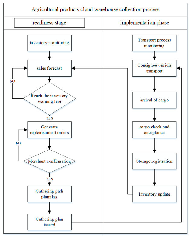
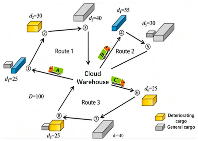
3.1. Smart Cloud Warehouse Consolidation Model for Agricultural Products

Given the volatility of the agricultural product market and seasonal fluctuations in demand, this study proposes a flexible and efficient inventory-management scheme. Rather than simply using a fixed proportion of the total inventory as the benchmark for safety stock, the monthly average sales volume was directly set as the safety stock level. This ensures that inventory levels can meet daily sales requirements without incurring unnecessary storage costs owing to excessive stockpiling. This study establishes a one-month lead time for restocking as a practical rule; the safety stock is used solely to trigger replenishment orders and is not claimed to be optimal in terms of inventory cost or stockout prevention. Let $I_i$ be the current inventory of product I at the beginning of month $t,F$ be the forecasted sales for month t and $S_i$ be the safety stock level. In this study, $S_i$ is set equal to the average monthly sales of the past 12 months. A replenishment order for product I is triggered if the inventory remaining after satisfying the forecasted demand would fall below the safety stock, i.e.,

$$I_i-F_i\le S_i$$

(2)

The replenishment quantity is set to $F_i$ (the forecast for the next month). This rule ensures that after meeting the expected demand, a buffer remains to cover unexpected sales. Following an analysis of the current smart cloud warehouse consolidation model for agricultural products, this study proposed a consolidated transport model based on sales forecasts. The specific collection process is illustrated in Figure 5, where vehicle routes are planned based on sales forecasts for agricultural products in order to provide consolidated transportation services to different merchants. The collection process for the smart cloud warehouse model for agricultural products is primarily divided into preparation and implementation phases. During the preparation phase, inventory levels are monitored in real time and monthly sales are forecasted to determine whether stock levels have reached the monthly stock alert threshold. Replenishment orders are generated for items expected to reach the stock alert threshold the following month and are sent to merchants. Once confirmed by merchants, the cloud warehouse can begin planning collection vehicle routes and formulating the collection schedule. Upon completion of the preparation phase, a collection plan is implemented. Vehicles are dispatched according to the plan to collect items and transport them back to the cloud warehouse, where the items are inspected and registered upon entry, before the inventory is updated.

3.2. Problem Description

The key to the operational model of a smart cloud warehouse for agricultural products is the vehicle route planning. The traditional consolidation model for cloud warehouses involves merchants arranging their dedicated transport based on their experience and demand to deliver items to the warehouse. This collection model is prone to stock build-up or stockouts when the demand fluctuates. Therefore, this study proposed a transportation collection model based on sales forecasts. It formulates carpooling routes and vehicle loading plans for merchants whose stock levels have reached the warning threshold in the smart agricultural product cloud warehouse, arranging for vehicles to depart from the distribution center at the end of each month to collect all items awaiting collection from designated locations and successfully load them into the vehicle. The vehicle routing problem for shared-load transport can be described as follows: The smart agricultural cloud warehouse serves as the distribution center, which has p vehicles of the same model, each with a cargo compartment of dimensions L × W × H and a maximum load capacity of Q. A cloud warehouse must provide collection services to customers within a city each month. The collection addresses and requirements of each customer were known. The number of items for the ith customer is denoted as mi, whereas the length, width, height, and weight of the kth item for that customer are denoted as l_ik, w_ik, h_ik, and b_ik, respectively. The distribution center dispatches vehicles to each customer’s premises, according to the collection schedule. Vehicles may commence loading upon arrival at any customer’s premises with no restrictions on the order or duration of visits. After collecting all items, the vehicles return to the distribution center to unload the cargo. Consequently, the route for each vehicle is a closed-loop path with the distribution center as both the starting point and destination, as illustrated in Figure 6. In this process, when planning the route, vehicles must consider the aggregate of various costs, including fuel consumption, carbon emissions, and empty-run penalties. Therefore, a single-objective route planning model is established in which all criteria (fixed vehicle cost, fuel cost, carbon emission cost, and empty-run penalty) are combined into a single monetary cost function. Load utilization is indirectly encouraged through the empty-run penalty, and carbon emissions are internalized via a carbon tax. The model thus balances economic and environmental objectives within a single scalar objective.

3.3. Basic Assumptions and Variable Definitions

3.3.1. Three-Dimensional Loading Assumptions

In view of the practical circumstances and research significance of three-dimensional loading and route planning for collection vehicles, the following assumptions are made:

(1)

Both the vehicle body and the items to be loaded are rectangular prisms.

(2)

The total weight and volume of items to be loaded from a single customer does not exceed the vehicle’s maximum weight and volume capacity.

(3)

When placing items, they must not be positioned at an angle and all edges of the items must be parallel or perpendicular to the sides of the vehicle.

(4)

After loading, the weight distribution is assumed to be relatively uniform. The center of gravity is not explicitly calculated, and no claim is made that the loading plans are physically safe under all conditions (e.g., during sharp turns or on uneven roads). The loading pattern is constrained by full support and stacking rules as geometric approximations, but these do not guarantee dynamic stability. This simplification is a major limitation of the current work, and the resulting loading plans should be interpreted as geometrically feasible rather than certified as operationally safe.

3.3.2. Collection Vehicle Route Planning Assumptions

(1)

The demand at each customer node is known and the collection requirements of all customers are met.

(2)

The demand is indivisible and each customer’s collection service must be completed in a single trip by the same vehicle.

(3)

The starting point and destination are at the same location, namely, the distribution center; each vehicle departs from the distribution center, completes the collection task, and returns to the distribution center.

(4)

Each route was completed by a single vehicle and each vehicle corresponded to a single driving route.

(5)

The specific coordinates of customers are known. The distance between nodes is approximated by the spherical (great-circle) distance calculated from latitude and longitude. This is a geometric simplification; the actual road distance may differ due to road networks, traffic conditions, and other factors. The distance between nodes is assumed to be constant for the purposes of this study.

(6)

Drivers possess identical driving skills. Vehicle speed is assumed to be constant (40 km/h) and is not affected by traffic conditions or other factors, as stated in Section 4.3.1. This simplification is accepted and the results are interpreted as an academic benchmark.

(7)

Carbon emission calculations only consider emissions generated during vehicle operation, specifically CO₂ emissions resulting from fuel consumption.

To ensure accuracy and clarity of expression, the relevant symbols and parameters of the constructed model are defined as

Table 5. Symbol definition and explanation.

Symbol	Definition	Notes
$i,j,h$	Node number
$J=\left\{0,\dots ,n\right\}$	$\mathrm{All} \mathrm{nodes}, \mathrm{where} i=0$ denotes the distribution center	set
$C=\left\{1,\dots ,n\right\}$	All customers	set
$P=\left\{1,\dots ,p\right\}$	All vehicles	set
$L,W,H$	Cargo compartment length, width and height	parameter
$l_{ik},w_{ik},h_{ik},b_{ik}$	Length, width, height and weight of the k-th consignment belonging to the i-th customer	parameter
$F_{fc}$	Fixed cost per vehicle	parameter
$F_{oc}$	Fuel consumption per unit distance when fully loaded	Parameter
$F_d$	Price of diesel	Parameter
$F_e$	Carbon tax	Parameter
$e_0$	CO2 emission factor	Parameter
$g^{\ast }$	Fuel consumption per unit distance when fully loaded	Parameter
$g_0$	Fuel consumption per unit distance when empty	Parameter
$Q$	Maximum payload of the vehicle	Parameter
$V$	Maximum volume of the cargo compartment	Parameter
$q_{ij}^p$	Real-time load of vehicle p from node i to node j	Parameter
$d_{ij}$	Distance from node i to node j	Parameter
$T{B}_i$	$\mathrm{Total} \mathrm{weight} \mathrm{of} \mathrm{cargo} \mathrm{at} \mathrm{node} \mathrm{i}, i\in C$	Parameter
$T{V}_i$	$\mathrm{Total} \mathrm{volume} \mathrm{of} \mathrm{cargo} \mathrm{at} \mathrm{node} \mathrm{i}, i\in C$	Parameter
$m_i$	Quantity of cargo for the i-th customer	Parameter
${\epsilon }_1$	Penalty cost for an empty vehicle	Parameter
$MT$	Maximum travel time per path	Parameter
$t_{ij}$	$\mathrm{Travel} \mathrm{time} \mathrm{from} \mathrm{node} \mathrm{i} \mathrm{to} \mathrm{node} \mathrm{j}, i,j\in V;i\ne j$ $\mathrm{and} t_{ij}=t_{ji}$	Parameter
$x_{ij}^p$	$\mathrm{Binary} \mathrm{variable}; 1 \mathrm{indicates} \mathrm{that} \mathrm{the} \mathrm{vehicle} \mathrm{travels} \mathrm{from} \mathrm{node} \mathrm{i} \mathrm{to} \mathrm{node} \mathrm{j}, i,j\in C$	Variable
$y_i^p$	$\mathrm{Binary} \mathrm{variable}; 1 \mathrm{indicates} \mathrm{that} \mathrm{the} \mathrm{vehicle} \mathrm{provides} \mathrm{the} \mathrm{service} \mathrm{from} \mathrm{node} \mathrm{i} \mathrm{to} \mathrm{node} \mathrm{j}, i,j\in C$	Variable

.

3.4. Development of a Route Planning Model for Consolidated Loading Under 3d Constraints

3.4.1. Analysis of the Objective Function

The objective function integrates four cost components: fixed vehicle cost, fuel consumption cost, empty-run penalty (which indirectly encourages high load utilization), and carbon emission cost. All components are expressed in monetary units (CNY) and summed with equal weighting (i.e., no additional scaling factors beyond the defined parameters). The empty-run penalty coefficient ε₁ is introduced in part (3) to control the trade-off between underutilization and total cost.

(1)

Fixed vehicle costs

Fixed vehicle costs refer to the fixed expenses directly associated with vehicle usage, including vehicle depreciation, insurance, driver wages, and routine maintenance costs. These costs are independent of vehicle mileage, fuel consumption, or cargo volume. The formula to calculate the fixed vehicle cost is as follows:

$$F_1=F_{fc}{\displaystyle {\displaystyle \sum }_{j=1}^C}{\displaystyle {\displaystyle \sum }_{p=1}^P}{x}_{0j}^p$$

(3)

(2)

Vehicle fuel consumption costs

Vehicle fuel consumption costs are determined by the amount of fuel consumed while the vehicle is in motion and are influenced by the load weight and distance traveled. To reflect real-world logistics scenarios, this study employs a dynamic fuel consumption model based on vehicle load weight to calculate fuel consumption. $F_{oc}\left(q_{ij}^p\right)$ represents the fuel consumption per unit distance when the vehicle $p$ carries a load on the $q_{ij}^p$ units. The formula for calculating vehicle fuel consumption cost is as follows:

$$F_2=F_d{\displaystyle {\displaystyle \sum }_{i,j=1}^C}{\displaystyle {\displaystyle \sum }_{p=1}^P}{F}_{oc}\left(q_{ij}^p\right)d_{ij}{x}_{ij}^p$$

(4)

$$F_{oc}\left(q_{ij}^p\right)=g_0+{\displaystyle \frac{g^{\ast }-g_0}{Q}}{q}_{ij}^p$$

(5)

(3)

Cost of vehicle underutilization

The actual loading capacity of a vehicle is subject to both volume and weight constraints, and its loading utilization rate depends on whether these two constraints reach their limits. Therefore, this study converts the vehicle load utilization rate into the cost of vehicle underutilization by setting a penalty coefficient of ${\epsilon }_1$; when a vehicle fails to fully utilize its weight or volume capacity, this unused capacity is regarded as a waste of resources. $T{B}_i$ represents the total weight of the items waiting to load at node i, whereas $T{V}_i$ represents the total volume of items waiting to load at node i. The formula for calculating the vehicle empty-run penalty cost is as follows:

$$F_3={\epsilon }_1{\displaystyle {\displaystyle \sum }_{p=1}^P}\left(1-\min \left({\displaystyle \frac{{{\displaystyle \sum }}_{i=1}^{C}T{B}_i{y}_i^p}{Q}},{\displaystyle \frac{{{\displaystyle \sum }}_{i=1}^{C}T{V}_i{y}_i^p}{L·W·H}}\right)\right)$$

(6)

$$T{B}_i={\displaystyle {\displaystyle \sum }_{k=1}^{m_i}}{b}_{ik}$$

(7)

$$T{V}_i={\displaystyle {\displaystyle \sum }_{k=1}^{m_i}}{l}_{ik}{w}_{ik}{h}_{ik}$$

(8)

The value ε₁ = 200 was selected based on a sensitivity analysis that tested ε₁ = 20, 200, and 2000 (see Section 5.3). While ε₁ = 2000 gives a slightly lower total cost, the improvement is marginal and the empty-run penalty becomes disproportionately high. ε₁ = 200 provides a balanced trade-off between load utilization and total cost, and is therefore used throughout this study.

(4)

Carbon emission cost

Fuel consumption during vehicle operation is the primary source of carbon emissions. The carbon emission cost is calculated as:

$$F_4={\displaystyle {\displaystyle \sum }_{i,j,p}^V}{\rho }_{ij}^p{d}_{ij}{E}_{oc}\tau$$

(9)

where ${\rho }_{ij}^p$ is fuel consumption (L/km), $d_{ij}$ is the distance from node i to node j (km), $E_{C{O}_2}=2.63kgC{O}_2/L$ is the emission factor, and $\tau$ is the carbon tax rate (CNY/kg CO₂). In this study, $\tau =0.334$ CNY/kg CO₂, which is equivalent to 0.88 CNY/L of diesel. Note that $C_{carbon}$ is proportional to fuel consumption; therefore, minimizing fuel consumption also minimizes carbon emissions. This design aligns economic and environmental incentives without introducing a separate trade-off.

Based on the analysis above, the objective function of the smart cloud warehouse vehicle route planning model for agricultural products developed in this study is as follows:

$$\begin{gathered} MinF=F_1+F_2+F_3+F_4=F_{fc}{\displaystyle {\displaystyle \sum }_{j=1}^C}{\displaystyle {\displaystyle \sum }_{p=1}^P}{x}_{0j}^p+F_d{\displaystyle {\displaystyle \sum }_{i,j=1}^C}{\displaystyle {\displaystyle \sum }_{p=1}^P}{F}_{oc}\left(q_{ij}^p\right)d_{ij}{x}_{ij}^p+ \\ {\epsilon }_1{\displaystyle {\displaystyle \sum }_{p=1}^P}\left(1-\max \left({\displaystyle \frac{{{\displaystyle \sum }}_{i=1}^{C}T{B}_i{y}_i^p}{Q}},{\displaystyle \frac{{{\displaystyle \sum }}_{i=1}^{C}T{V}_i{y}_i^p}{L·W·H}}\right)/p\right)+{\displaystyle {\displaystyle \sum }_{i,j,p}^V}{\rho }_{ij}^p{d}_{ij}{E}_{oc}\tau \end{gathered}$$

(10)

3.4.2. Analysis of Constraints

The constraints of the problem addressed in this study can be divided into vehicle route planning constraints and three-dimensional loading constraints.

(1)

Vehicle Route Planning Constraints

In route planning for collection vehicles in a smart cloud warehouse for agricultural products, vehicle route planning determines the basic routes, vehicle usage, and access sequences that serve as prerequisites for loading. The following are the vehicle route planning constraints used in this study.

$${\displaystyle {\displaystyle \sum }_{p=1}^P}{y}_i^p=1,i\in C$$

(11)

$${\displaystyle {\displaystyle \sum }_{i=1}^C}{x}_{ij}^p=y_j^p;{\displaystyle {\displaystyle \sum }_{j=1}^C}{x}_{ij}^p=y_i^p$$

(12)

$${\displaystyle {\displaystyle \sum }_{j=1}^C}{x}_{0j}^p={\displaystyle {\displaystyle \sum }_{i=1}^C}{x}_{i0}^p=1$$

(13)

$${\displaystyle {\displaystyle \sum }_{i=0}^V}{x}_{ih}^p={\displaystyle {\displaystyle \sum }_{j=0}^V}{x}_{hj}^p,h\in C$$

(14)

$${\displaystyle {\displaystyle \sum }_{i,j=0}^V}{x}_{ij}\le \left|V\right|-1$$

(15)

$${\displaystyle {\displaystyle \sum }_{j=1}^C}{\displaystyle {\displaystyle \sum }_{p=1}^P}{t}_{ij}{x}_{ij}^p\le MT$$

(16)

$$p\le n$$

(17)

$$x_{ij}^p\in \left\{0,1\right\},\forall i,j\in V,\forall p\in P$$

(18)

$$y_i^p\in \{0,1\},\forall i,\in C,\forall p\in P$$

(19)

In the model above, Equation (11) specifies that each customer is served by only one vehicle. Equation (12) specifies that each customer is served only once, and Equation (13) specifies that vehicles must depart from and return to the distribution center. Equation (14) specifies the subloop elimination constraint, whereby two merchants on a path must be connected by a single path with no subloops. Equation (15) represents the flow-balancing constraint, and Equation (16) represents the maximum travel time limit for each path. Equation (17) represents the upper limit of the number of vehicles. Equation (18) is a binary decision variable; if it is 1, it indicates that vehicle p travels from node i to node j. Equation (19) is a binary decision variable; if it is 1, it indicates that vehicle p performs the service from node i to node j.

(2)

Three-Dimensional Loading Constraints

In route planning for collection vehicles in smart cloud warehouses for agricultural products, three-dimensional loading constraints are established to ensure the rationality and feasibility of cargo loading while accommodating the specific physical properties and logistics requirements of agricultural products, thereby reducing cargo loss during transport and improving the loading efficiency. Three-dimensional loading constraints require cargo dimensions (length, width, and height) to be considered during the loading process, to ensure that items can be stacked rationally within the vehicle. This maximizes the utilization of the vehicle’s interior space, reduces empty space, and thereby improves the transport efficiency. Consequently, this study defines the vehicle’s interior as a three-dimensional space and establishes a coordinate system with the bottom-left rear corner of the vehicle as the origin (0,0,0), where the X-, Y-, and Z-axes correspond to the vehicle’s length, width, and height, respectively. Based on the above spatial and coordinate system definitions, this study proposes volume and load constraints, placement constraints, stacking constraints, support area constraints, and spatial non-overlap constraints to ensure that vehicles can load items efficiently.

a.

Volume and Load Constraints

Traffic regulations impose strict limits on vehicle load capacity; overloading may result in fines or the revocation of operating licenses. Because the volume and load capacity of a vehicle’s cargo compartment are fixed, exceeding the corresponding limits may lead to traffic accidents. Therefore, the volume and load constraints are the most fundamental among the three-dimensional loading constraints. The volume of the items within the cargo compartment must not exceed the maximum volume of the compartment, and the weight of the items must not exceed the maximum load capacity of the vehicle.

$${\displaystyle {\displaystyle \sum }_{i=0}^V}{\displaystyle {\displaystyle \sum }_{j=0}^V}T{V}_i{x}_{ij}^p\le V$$

(20)

$${\displaystyle {\displaystyle \sum }_{i=0}^V}{\displaystyle {\displaystyle \sum }_{j=0}^V}T{B}_i{x}_{ij}^p\le Q$$

(21)

b.

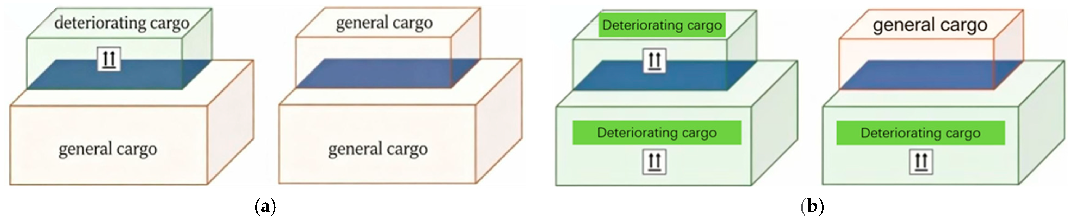
Stacking Constraints

Agricultural products include bulky items that are relatively large in volume but light in weight, such as dried green beans, and heavy items that are relatively small in volume but heavy in weight, such as rice, grains, and oil. There are significant differences in the physical properties of different agricultural products. Furthermore, some agricultural products are fragile, bulky items are prone to damage during transportation, and certain heavy items are susceptible to damage. Consequently, this study classifies agricultural products into general and fragile categories. All agricultural products have standardized external packaging, ensuring consistent dimensions and handling properties. Damage to fragile agricultural products can be effectively prevented by establishing the corresponding stacking constraints when stacking different items. A schematic diagram of the stacking process is shown in Figure 7, where (a) illustrates a stack that complies with the constraints and (b) illustrates one that does not. The specific stacking rules are as follows.

Rule 1: Any item type may be stacked on top of general items.

$$r_{ij}=1,if S_i^p=0$$

(22)

Rule 2: To prevent damage to items, this regulation stipulates that no other items should be stacked on top of fragile items.

$$r_{ij}=0,if S_i^p=1$$

(23)

In this context, $S_i^p$ = 0 indicates that the i-th type of cargo in the p-th vehicle is standard cargo, and $S_i^p$ = 1 indicates that the i-th type of cargo in the p-th vehicle is fragile. $r_{ij}=1$ indicates that cargo j can be stacked on top of cargo i and $r_{ij}=0$ indicates that cargo j cannot be stacked on top of cargo i.

c.

Support Area Constraints

The base of the cargo must have a sufficient support area to distribute pressure, which is particularly important for heavy agricultural production. An insufficient support area may cause the cargo to slide on bumpy roads, damaging other agricultural produce, and increasing the risk of breakage. To ensure the stability of the cargo arrangement, full support constraints must be considered during loading, that is, each item must be placed such that its base is fully supported. Therefore, this study determines whether items can be stacked by comparing their lengths, widths, and base areas.

$$l_i\ge l_j and w_i\ge w_j$$

(24)

$$l_i{w}_i\ge l_j{w}_j$$

(25)

where $l_i$ denotes the length of the i-th item, $w_i$ denotes the width of the i-th item, Equation (24) represents the constraints on the length and width, and Equation (25) represents the constraint on the base area. This is a geometric simplification: full support requires not only that the base of the upper item is smaller than the base of the lower item, but also that the weight distribution is such that the upper item’s projection lies entirely within the lower item’s surface. The present condition only checks the bounding rectangles; it does not verify actual contact area or alignment relative to the center of gravity. Consequently, the loading plans should be considered geometrically feasible but not guaranteed to be physically safe under all load distributions. This limitation is further noted in Section 5.1.

d.

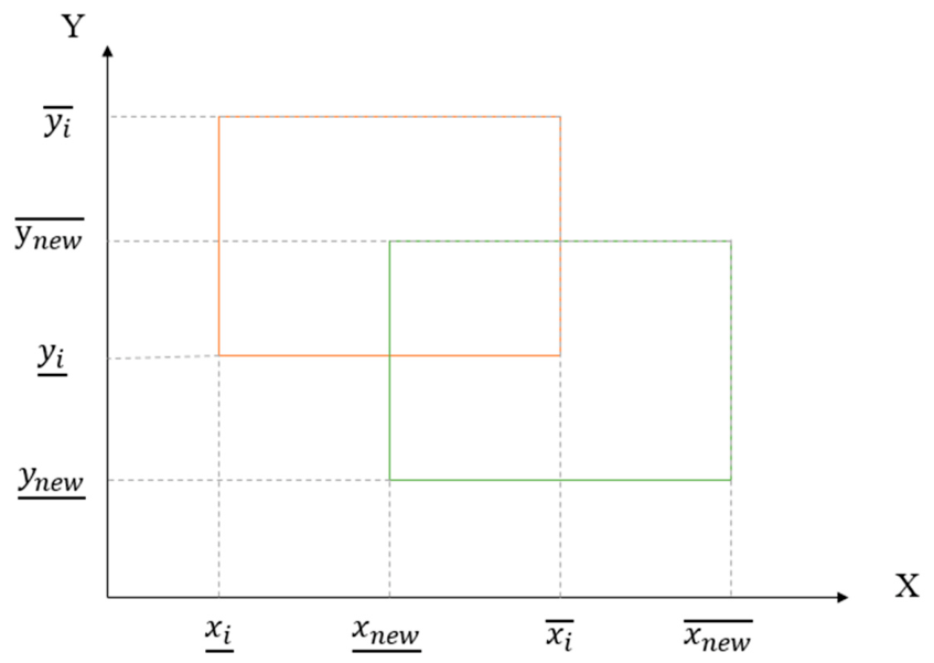
Spatial Non-Overlap Constraint

To prevent overlapping, a spatial non-overlap constraint is imposed. Two items are considered non-overlapping if their projections onto the XY-plane do not intersect. For two items a and b, let $\left(x_a^{bl},y_a^{bl}\right)$ and $\left(x_a^{tr},y_a^{tr}\right)$ denote the bottom-left and top-right coordinates of item $a^{\prime }s$ projection, respectively, and similarly for item b. The two projections do not overlap if any of the following four conditions hold:

$$x_a^{tr}\le x_b^{bl} \mathrm{or} x_b^{tr}\le x_a^{bl}{ \mathrm{or} \mathrm{y}}_a^{tr}\le y_b^{bl}{ \mathrm{or} \mathrm{y}}_b^{tr}\le y_a^{bl}$$

(26)

If none of these conditions is satisfied, the two rectangles overlap, which is forbidden. This condition is applied to every pair of items placed in the same vehicle. The projection of items onto the bottom of the carriage is illustrated in Figure 8.

4. Model Development Algorithm Design and Practical Implementation

4.1. Design of the Vehicle Route Planning Algorithm

In this study, a hybrid genetic–hill-climbing adaptive algorithm was designed to address the vehicle route planning problem. By employing a greedy strategy to generate a high-quality initial population, we introduce an adaptive crossover and mutation strategy to dynamically adjust the corresponding probabilities to increase population diversity and utilize an elite retention strategy to preserve superior individuals and accelerate convergence by combining the hill-climbing algorithm’s local search capability to compensate for the shortcomings of the genetic algorithm, thereby preventing the algorithm from becoming trapped in local optima and enabling a more accurate approximation of the global optimal solution.

Step 1: Initialize the parameters. Initialize the parameters of the genetic algorithm, including the initial population, maximum number of iterations G, crossover probability $p_c$ and mutation probability P_m. This study employed natural number encoding, where natural numbers represent the genes of a chromosome. A single chromosome represents a solution comprising the distribution center ID, merchant ID, and vehicle ID. Each merchant node is denoted by ‘1, 2, 3, …, n’, whereas the distribution center is denoted by n + 1.

Step 2: Initialize the population. In this study, the initial population is generated using a greedy strategy. First, the order of the merchant nodes is randomly shuffled. For each merchant, all possible insertion positions were attempted sequentially, and the insertion cost (i.e., the objective function value at each position) was evaluated. The position with the minimum objective function value is prioritized for insertion. If a feasible solution exists, it is inserted immediately. The greedy insertion process is performed independently for each individual in the population to generate distinct chromosomes.

Step 3: Fitness evaluation. As the objective of this study is to minimize the total cost, the reciprocal of the objective function is set as the fitness function, expressed as

$$F_n={\displaystyle \frac{1}{f_n}}$$

(27)

Here, F_n denotes the fitness value of individual n and fn denotes the total cost.

Step 4: Selection. Chromosomes were screened using the roulette-wheel method. In addition to proportional selection, this method was inspired by the principle of roulette wheels in casinos. The roulette wheel calculates the cumulative probability of each individual being selected based on its fitness value, and maps these probabilities to various sectors of the wheel. By spinning the wheel, the individuals correspond to the sector in which the pointer lands are retained and used for subsequent operations.

Step 5: Crossover. An adaptive crossover probability is employed; this probability is not fixed but is dynamically adjusted as the algorithm runs. The formula for the adaptive crossover probability is as follows:

$$P_c=\left\{\begin{array}{c}{\displaystyle \frac{P_{cb}\left(f_1-f_{avg}\right)}{f_{max}-f_{avg}}},f_1\ge f_{avg}\\ P_{cb}, f_1<f_{avg}\end{array}\right.$$

(28)

where P_c denotes the adaptive crossover probability, P_cb = 0.8 denotes the basic crossover probability, f₁ denotes the fitness value of an individual, f_avg denotes the average fitness of the population, and f_max denotes the maximum fitness of the population.

Step 6: Mutation. Two mutation sites were randomly selected, and the genes at these two sites were swapped. The mutated individuals then become offspring. This is because as the algorithm iterates continuously, the individuals in the population become increasingly similar, leading to a gradual narrowing of the search space and making it difficult to discover new optimal solutions. When no new optimal individuals are produced for several consecutive generations, the algorithm must apply a relatively high mutation probability. By increasing the mutation rate, the diversity of individuals in the population can be enhanced, thereby enabling the algorithm to escape the current local optimum region. The formula for adaptive mutation probability is as follows:

$$P_m=\left\{\begin{array}{c}{\displaystyle \frac{P_{mb}\left(f_1-f_{avg}\right)}{f_{max}-f_{avg}}},f_1\ge f_{avg}\\ P_{mb}, f_1<f_{avg}\end{array}\right.$$

(29)

Here, P_m denotes the adaptive mutation probability, P_mb = 0.01 denotes the basic mutation probability, f₁ denotes the fitness value of an individual, f_avg denotes the average fitness value of the population, and f_max denotes the maximum fitness value of the population.

Step 7: Hill-climbing algorithm. We randomly select two genes from merchant nodes, swap the positions of these two genes to generate a neighboring solution, and evaluate the fitness of the neighboring solution. If the fitness of the neighboring solution is superior to that of the current individual, replace the individual; otherwise, retain it. The algorithm iterates through each individual and performs independent local optimization until no better individual can be found, at which point the hill-climbing algorithm terminates.

Step 8: Elite retention strategy. The elite retention ratio is typically set to 0.05; a ratio that is too high may affect the population diversity, whereas a ratio that is too low may lose its retention value. Assuming a population size of 100, a new population was obtained after performing selection, crossover, mutation, and hill-climbing operations on the population. The fitness of the population was evaluated and ranked and the top five elite individuals were retained at a ratio of 0.05. These five elite individuals were merged with the population of the previous generation. After reranking, the top 100 individuals were selected to form the new population for iteration.

4.2. Design of the 3D Loading Verification Algorithm

4.2.1. Loading Rule

Taking into account the constraints of 3D loading, this study adopts the concept of ‘stacks’ to arrange stacking groups on a 2D plane. In other words, while satisfying the height constraints, the 3D loading problem was simplified into a 2D layout problem by stacking items of the same type and combining the different types into stacks. Based on placement rules, stacking and merging rules, and two-dimensional loading rules, this study designed a three-dimensional loading verification algorithm comprising primarily homogeneous stacking, stacking, and merging, and a two-dimensional layout.

4.2.2. Placement Rules

In addition to the requirement that the edges of the cargo must be orthogonal or parallel to the vehicle body, constraints stipulate that the cargo must be placed upright (not inverted) and may only be rotated by 90°.

(1)

Stacking And Merging Rules

The stacking rules for fragile items require special handling measures during the stacking process. By establishing stacking and merging rules, this study simplifies the verification process for fragile items, which only needs to be carried out during the stacking and merging process, effectively avoiding the need for the algorithm to repeatedly check fragile attributes of items during the placement stage.

The stacking and merging rules implement the stacking rules for items using a combination scoring method with the following scoring formula:

$$Scor{e}_{combined}=base\_area-\epsilon \ast if\_fragile$$

(30)

Here, base_area represents the base area of the stacking group, ε represents the penalty coefficient, and fragile is a decision variable assigned a value of 1 if the stacking group contains fragile items and 0 otherwise.

The scoring rules award points based on the base area of the stacking group, whereas fragile stacking groups have points that are deduced via the penalty coefficient. Consequently, stacking groups with a larger base area and no fragile items were prioritized in the scoring process and given priority for handling. Even stacking groups with a large base area that contain fragile items will reduce their priority owing to penalty points.

(2)

Improved Two-Dimensional Loading Rules

Given the established placement rules, namely that items cannot be inverted and there are only two possible rotation directions, it is evident that only the length and width constraints must be considered when placing items. This study reduced the three-dimensional loading to two-dimensional loading, thereby further simplifying the algorithmic process.

In the process of optimizing the two-dimensional layout, this study integrates the principles of the BL and BF algorithms to guide the placement of stacking groups. First, based on the principle of descending base areas, stacking groups with larger base areas are prioritized, creating larger contiguous spaces for subsequent stacking groups and preventing small items from occupying advantageous positions. Second, the candidate placement points were generated. When no items were loaded, the initial placement point was set as the origin (0, 0) of the coordinate system. When the loading space contained items, the placement point was set at the right and top boundary points of the base of the previously placed stacking group. Finally, a comprehensive spatial quality evaluation function was designed for the placement strategy that integrates the BL and BF algorithms.

$$Scor{e}_{waste}=\left(x+y\right)+\min \left\{L-\left(x+l\right),W-\left(y+w\right)\right\}$$

(31)

Here, x and y denote the coordinates of the placement point; L and W represent the length and width of the carriage, respectively; and l and w represent the length and width of the base area of the newly placed stack, respectively. (x + y) represents the distance from the bottom-left corner of the stacking group to the origin; the smaller this distance, the better, because it encourages the items to cluster towards the bottom-left corner. Min{L-(x + l), W-(y + w)} represent the minimum distance from the top-right corner of the stacking group base to the right or top boundary of the loading space, respectively. The smaller the distance, the better, because it encourages the stacking group to remain close to the boundaries of the loading space.

4.2.3. Algorithm Structure

First, each cargo type is vertically stacked and grouped, and the height and position information for each stack are calculated and stored. Second, stacks of different types are merged into larger stacks, according to the rules. Subsequently, a two-dimensional layout is created for the merged stacks. Finally, the final coordinates of all cargoes are updated based on the results of the two-dimensional layout.

(1)

Stacking of the Same Type

The vertical stacking of items of the same type reduces the horizontal footprint, while ensuring that the total stack height does not exceed the specified maximum height. The specific steps are as follows.

Step 1: Create a new stacking group index list, initialize the stacking group to include the item ID and stacking group height, and fix the item orientation.

Step 2: If the current cargo ID is less than or equal to the total number of cargo items, proceed to Step 2.1. If the current cargo ID exceeds the total number of cargo items, proceed to step 4.

Step 2.1: Calculate the sum of the stacking groups and box heights. If this sum is less than or equal to the vehicle height, add the current cargo item to the stacking group index list; if the sum exceeds the vehicle height, stop adding and proceed to Step 3.

Step 2.2: Update the stacking group index and height.

Step 3: Check if the current stacking group index list is empty. If it is not empty, proceed to step 4. If it is empty, terminate the current code; otherwise, stop stacking.

Step 4: Store the current stacking group index and height in the stacking group.

Step 5: The cargo stacking process is complete; stacking successful.

(2)

Stacking of Different Types

When stacking different types of cargo, non-fragile items are prioritized in the overall scoring, whereas fragile items are placed at the top or are stacked separately to prevent damage. The specific steps are as follows.

Step 1: The dimensions, height, type, and original index of all the stacking groups were retrieved.

Step 2: The base area for each stacking group is calculated. We calculate a score based on the base area and priority of fragile items, prioritize non-fragile items, and sort the stacking group indices in descending order.

Step 3: Iterate by stacking the groups. If stacking group i (where i starts from 1) has already been processed, skip the current stacking group and continue the iteration. If it has not been processed, create a new merged stacking group and mark i as processed.

Step 4: Stack the subsequent stacking group j (starting from i + 1) onto the stacking group i. If this stacking group has already been processed, skip it and continue the traversal; if it has not been processed, proceed to Step 5.

Step 5: Check whether the merged stacking group satisfies stacking constraints. If so, proceed to Step 6; otherwise, disallow the merge, and return to Step 4.

Step 6: Check whether the merged stacking group satisfies the full support and height constraints. If satisfied, proceed to Step 8; if not, proceed to Step 7.

Step 7: Rotate the stacking group by 90° and perform the merge stack operation. Re-check full support and height constraints. If satisfied, perform the merge stack operation and mark the rotation direction; if it is still unsatisfactory after rotation, skip the stacking group.

Step 8: Mark j is processed and the information of the newly merged stacking group is recorded.

Step 9: Iterate all stacking groups and add any unprocessed stacking groups to the information of the newly merged stacking group.

(3)

Two-Dimensional Layout

After merging items into stacking groups by combining stacks of the same type and stack combinations, the three-dimensional stacking groups can be treated as two-dimensional rectangles. When performing the planar layout, prioritizing rectangles with larger base areas and conducting a comprehensive assessment of the quality of the remaining space can improve overall space utilization. The specific steps are as follows.

Step 1: Initialize the indices and dimensions of the placed rectangles.

Step 2: Calculate the base area of each stacking group, sort them in descending order of base area, and save the indices before sorting.

Step 3: Iterate through the sorted stacking groups.

Step 3.1: Attempt placement in the default orientation. If this orientation satisfies the non-overlapping constraint and the position does not exceed the vehicle boundaries, proceed to Step 3.3; otherwise, proceed to Step 3.2.

Step 3.2: Attempt placement with rotated orientation. If this orientation satisfies the non-overlapping constraint and the position does not exceed the vehicle boundaries, proceed to Step 3.3; otherwise, the placement fails.

Step 3.3: Search for the optimal placement point. The remaining space was scored according to the two-dimensional loading rules, and the point with the lowest score was selected as the optimal placement point.

Step 4: Successful placement. The coordinates and orientation were recorded and a stacking group was added to the index of the rectangles.

4.2.4. Handling of Loading Failures and Feedback to Route Planning

When a candidate route fails the 3D loading verification (e.g., volume exceedance, stacking violation, or support area insufficiency), the algorithm does not attempt to repair or reorder the items. Instead, it applies a penalty-based filter with a short-term memory. Specifically, a large penalty cost (P_fail = 10,000 CNY) is added to the total cost of that route in the objective function (Equation (10)). This penalty makes infeasible routes less likely to survive in the selection step of the genetic algorithm.

In addition, the algorithm records the specific cause of failure in a “failure memory”. For each failure, we store a pair of item identifiers (i, j) that were placed in the same vehicle and contributed to the violation (e.g., a fragile item stacked under a heavy box). The memory retains the most recent 10 generations of such item pairs, after which older entries are discarded. During the mutation operator of subsequent generations, when two items are selected to be swapped, the algorithm checks whether the pair (i, j) exists in the failure memory. If it does, the swap is accepted with a reduced probability (50% of the normal acceptance rate), thereby biasing the search away from repeatedly generating the same infeasible combination. This bias is soft (not a hard constraint), because a pair that was infeasible in one route order may become feasible if the visit sequence or stacking order changes. The memory is reset after every 50 generations to avoid permanent over-constraint.

Thus, the algorithm does not implement a tight coupling between routing and loading; it uses a penalty filter augmented with a short-term memory of problematic item pairs. This approach is sufficient to guide the genetic search toward feasible route-loading combinations without the computational cost of explicit repair or reordering. The name “path planning–loading verification” in the two-stage framework is kept for consistency, but the mechanism is essentially a penalty filter with memory.

The following pseudocode summarizes the penalty filter with memory. The Algorithm 1 distinguishes between two types of failures: (i) stacking violations, where a specific pair of items (e.g., fragile under heavy) causes the failure—such pairs are stored and used to bias mutation; and (ii) volume or weight exceedances, which are treated as global failures without storing item pairs, as they depend on the total load rather than a specific combination.

Algorithm 1: Penalty filter with memory for loading failures

Input: Candidate route R (sequence of merchants, each with item set I_i) Output: Updated cost and failure memory M 1.    Perform 3D loading verification on route R. 2.    IF verification succeeds:                   Accept route with normal cost.                   Return. 3.    ELSE: // loading failure                   Add penalty P_fail = 10,000 CNY to total cost of R.                   Determine failure type:                           IF failure is stacking violation (fragile under heavy):                                   Identify the two items causing violation: (i_fragile, j_heavy)                                   Store pair (i_fragile, j_heavy) into memory M with current generation counter.                           ELSE IF failure is volume or weight exceedance:                                   Do not store any item pair (the violation is global).                   // Update memory: keep only most recent 10 generations                   FOR each pair in M:                           IF current_generation—pair.generation > 10:                                   Remove pair from M.                   // Prevent mutation from repeating same infeasible combination                   Record R as infeasible. 4.    During mutation operator of subsequent generations:                 IF a swap would place items (a,b) that exist in M into same vehicle:                           Accept the swap with probability 0.5 (otherwise reject).                 ELSE:                           Accept with normal probability. 5.    Every 50 generations, reset M to empty.

4.3. Example of Solving the Route Planning Algorithm for Smart Cloud Warehousing of Agricultural Products

4.3.1. Data Collection

We acknowledge that using spherical distance (haversine formula) as a proxy for actual road distance is a simplification. Real urban logistics are affected by road networks, traffic congestion, one-way streets, and winter conditions. The constant speed assumption (40 km/h) further abstracts away travel time variability. Therefore, the results of this case study should be interpreted as an academic benchmark rather than an operational guarantee. Future work should incorporate actual road distance matrices and dynamic travel times.

(1)

Receiving nodes and distance data

Based on the monthly sales data for agricultural products, sales data from merchants whose total product weight and volume exceeded the load and volume limits of a single vehicle were excluded. The location and item information of merchants that reached the stock warning level in January were collected. This study involved 48 merchants who required collection, corresponding to 62 items. Because supplier addresses involve merchant privacy, the collection locations for some merchants are the actual addresses of the item suppliers, whereas the collection locations for the remaining merchants are set as simulated addresses. All collection points were located within Harbin City and its subordinate districts and counties, with detailed address information including administrative level identifiers such as provinces, cities, districts, and streets. The specific coordinates of merchants as well as the geographical locations of the cloud warehouse and merchants are known. The spherical distance (great-circle distance) between nodes is calculated using the DISTDIM function in MATLAB R2022a and used as a proxy for the transport distance, acknowledging that actual road distances may differ.

(2)

Item Data

For merchants that reached the inventory warning threshold, data from on-site surveys were collected regarding the loading dimensions, including the length, width, and height of the packaging, weight, and loading specifications. The nature of the items was also recorded, with fragile items assigned a value of 1 and non-fragile items assigned a value of 0.

(3)

Vehicle Data

The agricultural smart cloud warehouse’s own delivery fleet consists of 9.6-m box-type express delivery vehicles. The cargo compartment dimensions are 9.5 × 2.5 × 2.5 m, with a gross vehicle weight of 25,000 kg and a maximum rated payload of 17,000 kg. The fuel consumption per unit distance when fully loaded was 27 L/100 km and the fuel consumption per unit distance when empty was 13 L/100 km. The vehicles in this study were assumed to travel at a constant speed of 40 km/h in accordance with the latest notice issued by the Harbin Municipal Public Security Traffic Administration.

4.3.2. Solution Results

The algorithm parameters were set based on preliminary experiments and a grid search on a validation instance.

Table 6. Parameter settings for the optimization model and algorithms.

Category	Parameter	Symbol	Value	Unit
Vehicle and Cost	Fixed cost per vehicle	$C_{fixed}$	500	CNY/vehicle
	Diesel price	$P_{diesel}$	7	CNY/L
	Carbon emission factor	$E_{C{O}_2}$	2.63	kg CO2/L diesel
	Carbon tax	$\tau$	0.334	CNY/kg CO2
	Fuel consumption	${\rho }_{full}$	0.27	L/km
	Fuel consumption	${\rho }_{empty}$	0.13	L/km
	Empty-run penalty coefficient	${\epsilon }_1$	200	dimensionless
Vehicle Constraints	Maximum payload	$Q_{\max }$	17,000	kg
	Maximum cargo volume	$V_{\max }$	59.375	m3
	Maximum working time per route	$T_{\max }$	8	h
	Vehicle speed (constant)	$v$	40	km/h
Algorithm (GA and Hybrid)	Number of iterations	$G$	1000	-
	Population size	$N_{pop}$	200	-
	Base crossover probability	$P_{cb}$	0.8	-
	Base mutation probability	$P_{mb}$	0.01	-
	Elite retention ratio	$P_{elite}$	0.05	-
	Hill-climbing selection ratio	$r_{hc}$	0.2	-
Algorithm (Simulated Annealing)	Initial temperature	$T_{init}$	100	-
	Cooling rate	$\beta$	0.99	-
	Termination temperature	$T_{end}$	0.01	-

summarizes all parameter values used in this study.

This study used MATLAB to solve the route planning model for agricultural smart cloud warehouse collection vehicles. During the computational process, a 3D loading verification algorithm was applied to each collection route generated by the algorithm to verify whether each route could be successfully loaded while satisfying 3D loading constraints. Building upon the existing literature and incorporating the actual conditions of the smart cloud warehouse for agricultural products, along with multiple experimental calculations, the algorithm parameters set in this study are listed in Table 6.

The parameters of the genetic algorithm (population size, crossover probability, mutation probability) and simulated annealing (initial temperature, cooling rate, iterations per temperature) were determined via a systematic grid search using a separate validation instance derived from historical data (December 2024). The following ranges were searched: population size {100, 150, 200, 250}, base crossover probability {0.7, 0.8, 0.9}, base mutation probability {0.005, 0.01, 0.02}, initial temperature {50, 100, 200}, cooling rate {0.95, 0.99, 0.995}. The combination yielding the lowest average total cost over five runs was selected. For the hybrid algorithm, the same GA parameters were used as for the standalone GA to ensure fair comparison. The hill-climbing local search was applied to 20% of randomly selected individuals in each generation after crossover and mutation, as this ratio yielded the best trade-off between solution quality and runtime in preliminary experiments.

The cargo collection route planning algorithm designed by the research team was applied to solve the route planning problem of a smart cloud warehouse for agricultural products. After 1000 iterations, the optimal collection routes and three-dimensional loading schemes were obtained.

The empty-run penalty coefficient was set to ε₁ = 200, which was determined by the sensitivity analysis presented in Section 5.3. This choice ensures a good compromise between vehicle load utilization and total cost. According to the collection route planning results in

Table 7. Optimal consolidation path.

Vehicle	Route	Fuel Cost (CNY)	Empty-Run Cost (CNY)	Carbon Emission Cost (CNY)	Load Utilization Rate (%)	Volume Utilization Rate (%)
1	49-7-29-34-3-49	156.48	64.12	19.65	67.94	70.47
2	49-37-1-49	113.57	57.54	14.26	84.00	71.23
3	49-33-13-17-49	63.72	24.92	8.00	99.58	87.54
4	49-20-12-46-49	161.50	33.09	20.28	88.80	83.45
5	49-45-9-41-49	131.25	96.44	16.48	95.98	51.78
6	49-6-36-23-49	106.01	40.65	13.31	91.32	79.67
7	49-47-30-49	166.19	98.73	20.86	89.59	50.63
8	49-40-38-49	187.02	78.11	23.48	85.77	60.94
9	49-2-31-49	120.06	71.67	15.07	99.14	64.16
10	49-48-26-49	182.81	66.89	22.95	98.24	66.55
11	49-4-32-49	114.64	66.34	14.39	98.99	66.83
12	49-43-22-49	86.21	64.34	10.82	95.87	67.83
13	49-44-15-49	232.95	59.35	29.25	93.06	70.32
14	49-10-21-49	190.29	66.64	23.89	66.68	72.43
15	49-5-39-49	169.12	54.61	21.23	91.47	72.69
16	49-28-18-49	76.07	49.39	9.55	95.48	75.30
17	49-16-11-49	187.61	41.91	23.55	90.26	79.04
18	49-19-42-24-49	121.60	33.42	15.27	90.08	83.29
19	49-8-14-49	74.78	32.13	9.39	92.09	83.93
20	49-25-35-27-49	135.52	28.20	17.01	89.65	85.90

, the transport task involved 20 routes. Based on this, the cloud warehouse must complete collection tasks at 48 location nodes via 20 transport trips with a total cumulative cost of 14,254.40 yuan. The average fuel cost per transport trip is 138.87 yuan, the average carbon emission cost is 17.43 yuan, and the average empty-run cost is 56.43 yuan. The average load utilization rate was 90.20%, with a maximum load utilization rate of 99.58%. The minimum load, average volume, maximum volume, and minimum volume utilization rates were 66.67%, 72.20%, 87.54%, and 50.63%, respectively.

A schematic of the loading plans for routes 1–6 is shown in Figure 9. The loading plans included a list of all items to be collected from each merchant as well as a layout diagram showing the positioning of different items. The collection route map is shown in Figure 10, where ‘49’ represents the cloud warehouse and 1–48 represents the collection nodes, which illustrates the optimal collection route, with the cloud warehouse serving as both the starting point and destination.

4.3.3. Comparison of Solution Results

To further verify the effectiveness of the improved genetic algorithm in solving the vehicle route planning problem under three-dimensional loading constraints, this study employed both a genetic algorithm and a simulated annealing algorithm to solve the collection route planning model. To ensure the validity of the comparison results, the initial temperature was set to 100 and the termination temperature was set to 0.01, ensuring that the temperature did not reach the termination condition prematurely. Furthermore, a temperature decay coefficient of 0.99 was set to slow the rate of temperature decline, thereby ensuring that the simulated annealing algorithm would undergo 1000 iterations. A comparison of the results of the hybrid algorithm with the iteration curves and those of the simulated annealing and genetic algorithms is presented in Figure 11 and

Table 8. Comparison of single-run results of GA, SA, and the hybrid algorithm.

Metric	Genetic Algorithm	Hybrid Algorithm	Simulated Annealing Algorithm
number of routes	23	20	21
total fuel cost (CNY)	2938.22	2777.40	2997.21
empty-run cost (CNY)	1786.44	1128.49	1418.65
average load utilization rate (%)	78.43	90.20	85.90
maximum load utilization rate (%)	91.39	99.58	96.48
average volume utilization rate (%)	62.78	72.20	68.76
maximum volume utilization rate (%)	85.22	87.54	87.52
total carbon emissions cost (CNY)	369	348.5	376.3
total cost (CNY)	16,593.7	14,254.4	15,292.2
algorithm runtime (seconds)	1311	1180	932

.

As shown in Figure 11 and Table 8, the simulated annealing algorithm converged relatively quickly, followed by the hybrid and the genetic algorithm. A comparative analysis of the data in the table reveals significant differences between the genetic algorithm, hybrid algorithm, and simulated annealing algorithm in solving the route planning model for the collection of agricultural products in a smart cloud warehouse; the hybrid algorithm demonstrated the best overall performance, and the simulated annealing algorithm offered the best timeliness, while the genetic algorithm performed relatively poorly overall. In terms of the solution duration, the simulated annealing algorithm was the most time-efficient, followed by the hybrid and genetic algorithms. Compared with the genetic algorithm, the hybrid algorithm reduces total cost by 2339.3 CNY (14.1%) and compared with simulated annealing, it reduces total cost by 1037.8 CNY (6.8%), respectively. The core advantage lies in the reduction in empty-run costs. Through more efficient route integration and vehicle scheduling, the hybrid algorithm achieved higher resource utilization rates, namely, an average load utilization rate of 90.20%, an average volume utilization rate of 72.20%, a maximum load utilization rate of 99.58%, and a maximum volume utilization rate of 87.52%. In contrast, the genetic algorithm resulted in the highest total cost owing to higher empty-run costs and lower load utilization rates, while simulated annealing, although the fastest to run, still incurred a higher total cost than the hybrid algorithm owing to insufficient vehicle load utilization rates and higher fuel consumption costs. In terms of environmental benefits, by controlling fuel consumption costs, the hybrid algorithm reduced carbon emission costs by 20.5 yuan compared to the genetic algorithm and by 27.8 yuan compared to simulated annealing. Based on the comparison of the results and the above analysis, it can be concluded that when considering economic, environmental, and load utilization rates comprehensively, the genetic–hill-climbing adaptive hybrid algorithm is more effective than the other algorithms in solving the route planning model for the smart cloud warehouse collection of agricultural products. It can achieve successful loading of all vehicles within an acceptable solution time, while providing a more precise and optimized collection route plan. This validates the applicability of the proposed model and algorithm to research problems and practical cases.

To ensure statistical reliability, each algorithm (GA, SA, and the proposed hybrid) was run 30 times independently on the same instance. All runs were conducted on the same hardware. For each algorithm (GA, SA, hybrid), we generated 30 different random seeds. The same set of 30 seeds was used for all three algorithms to enable paired comparisons. The Wilcoxon signed-rank test was performed as follows: For each random seed (1 to 30), we paired the total cost of the hybrid algorithm with that of GA (and separately with SA). The differences were ranked by absolute value, and the test statistic W was computed. No correction for multiple comparisons was applied because only two pairwise tests were conducted. The resulting p-values were below 0.01 for both comparisons, indicating that the hybrid algorithm significantly outperforms the benchmarks. The test statistics were W = 435 (GA vs. hybrid) and W = 412 (SA vs. hybrid), both above the critical value for α = 0.01 with 30 pairs.

Table 9. Statistical comparison of algorithms over 30 independent runs.

Algorithm	Metric	Mean ± Std	Best	Worst	p-Value (vs. Hybrid)
GA	Total Cost (CNY)	16,543.8 ± 210.5	16,444.1	16,913.6	<0.01
	Avg. Load Util. (%)	78.10 ± 2.10	78.80	75.1
SA	Total Cost (CNY)	15,301.7 ± 188.7	15,261.1	15,666.7	<0.01
	Avg. Load Util. (%)	85.50 ± 1.90	86.20	82.4
Hybrid	Total Cost (CNY)	14,266.7 ± 145.3	14,254.4	14,524.6	-
	Avg. Load Util. (%)	90.00 ± 1.50	90.2	87.6

reports the mean, standard deviation, best, and worst values of total cost and average load utilization over these 30 runs.

All algorithms were implemented in MATLAB R2022a and run on a workstation with an Intel Core i7-12700K CPU (3.6 GHz) and 32 GB RAM. The same initial population and random seeds were used for GA and the hybrid algorithm to ensure fair comparison. Simulated annealing was configured with an initial temperature of 100, cooling rate of 0.99, and termination temperature of 0.01, which resulted in approximately 1000 iterations per run.

Each algorithm was run 30 times with different random seeds. The p-values are from the Wilcoxon signed-rank test. The hybrid algorithm’s failure rate in 3D loading verification was 4%, compared to 12% for GA and 8% for SA.

The hybrid algorithm achieves the lowest mean total cost and highest mean load utilization, with the smallest standard deviation, indicating both better performance and higher stability. The Wilcoxon signed-rank test confirms that the differences between the hybrid algorithm and both GA and SA are statistically significant (p < 0.01). These results provide strong evidence that the proposed hybrid algorithm outperforms the benchmark methods consistently, not merely due to random initialization or parameter tuning.

4.3.4. Value of Forecasting Integration: A Counterfactual Analysis

To assess the true contribution of the forecasting module, we conducted a counterfactual experiment using ex-post actual demand data. Specifically, after the collection operations for January 2025 were completed, we obtained the actual sales volumes of all 48 merchants. We then re-ran the entire route planning model using these actual demand values as input, while keeping all other parameters identical. The resulting ‘ex-post optimal plan’ represents the best achievable outcome if demand were perfectly known in advance. Comparing this plan with our forecast-driven plan reveals the performance gap attributable to forecasting errors (

Table 10. Comparison between forecast-driven plan and ex-post optimal plan.

Metric	Forecast-Driven Plan	Ex-Post Optimal Plan
Total Cost (CNY)	14,254.40	13,546.23
Number of Routes	20	19
Avg. Load Utilization (%)	90.20	93.50
Carbon Cost (CNY)	348.52	332.00

).

The ex-post plan achieves a 4.97% lower total cost, primarily due to a reduction in one route and higher load utilization (from 90.20% to 93.50%). Further analysis revealed that 68% of the cost gap originated from three merchants whose sales were unexpectedly boosted by unrecorded promotional events. This suggests that incorporating external covariates (e.g., holidays, promotions) into the forecasting model could further close the gap. Nevertheless, the forecast-driven plan still performs within 5% of the theoretical optimum, demonstrating the practical value of integrating sales forecasting even in the presence of prediction uncertainty. These results are not in contradiction with the safety buffer mentioned in Section 2.3: the safety stock absorbs only routine random fluctuations, whereas the counterfactual experiment reveals the effect of larger, systematic forecasting biases (e.g., unrecorded promotions) that are not covered by the safety buffer. Hence, the two statements are complementary rather than contradictory.

5. Discussion

5.1. Discussion and Limitations

In this section, the sales forecasting and collection path planning methods proposed in this study are discussed in-depth. First, the effectiveness and innovation of the method were analyzed from four aspects: prediction accuracy, loading adaptability, algorithm performance, and environmental economic coordination. Second, it objectively highlights the limitations of this study and proposes directions for improvement in future work.

(1)

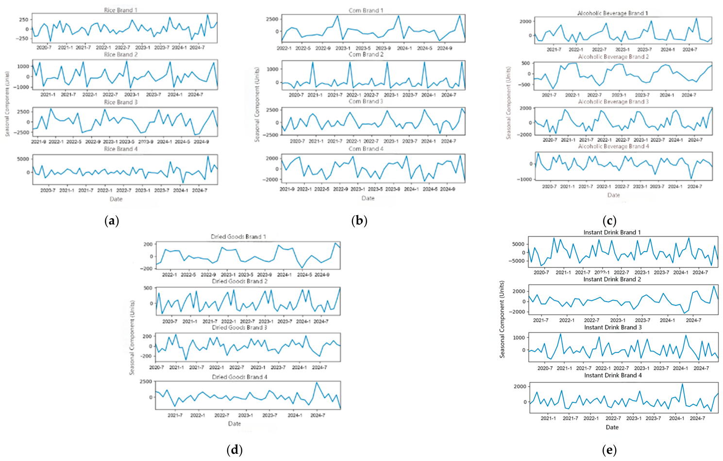
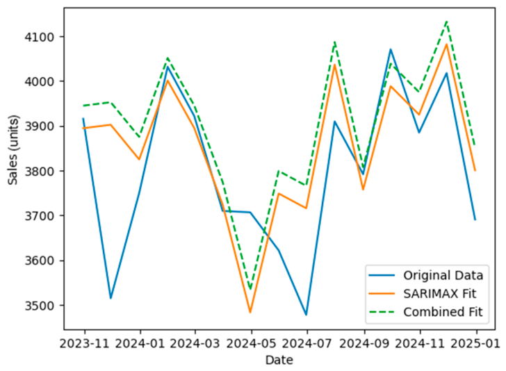
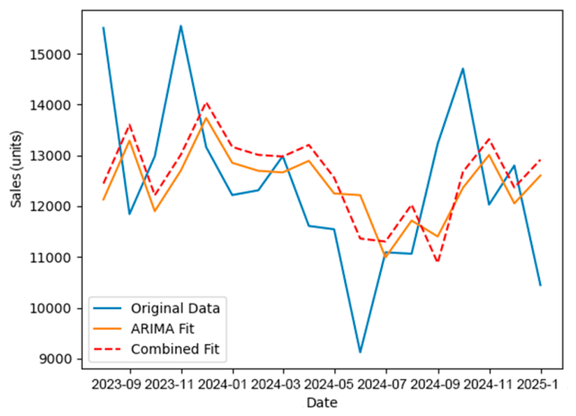
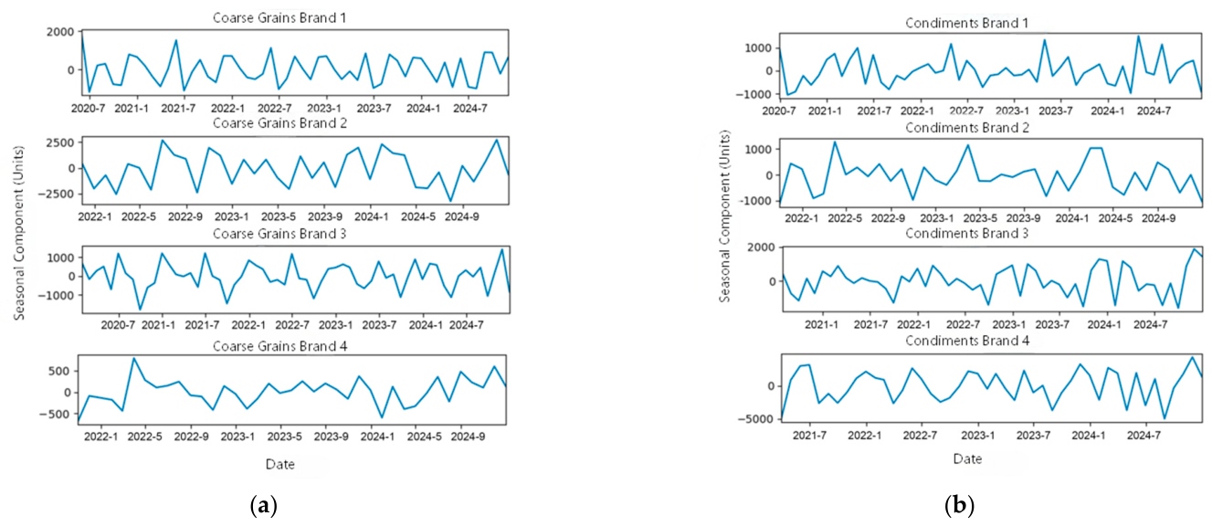
The SARIMA/ARIMA-BPNN combined forecasting model constructed in this study identifies the seasonal characteristics of agricultural product sales through STL decomposition and separately models the linear trends and nonlinear residuals. The experimental results show that for commodities with obvious seasonality (such as rice and corn), the MAPE of the combined model is as low as 3.50%, which is approximately 15% lower than that of the SARIMA model alone. For non-seasonal commodities (coarse grains and condiments), the MAPE values were 9.50% and 12.38%, respectively, all below the 15% threshold. This indicates that the combined model can be adapted to the demand fluctuation law for the different categories of agricultural products. The prediction results of this study are directly used to trigger the monthly inventory warning line and generate replenishment orders, which establishes a data-driven connection between demand forecasting and path planning. No claim is made regarding the optimality of this inventory rule in terms of storage costs or lost sales prevention.

(2)

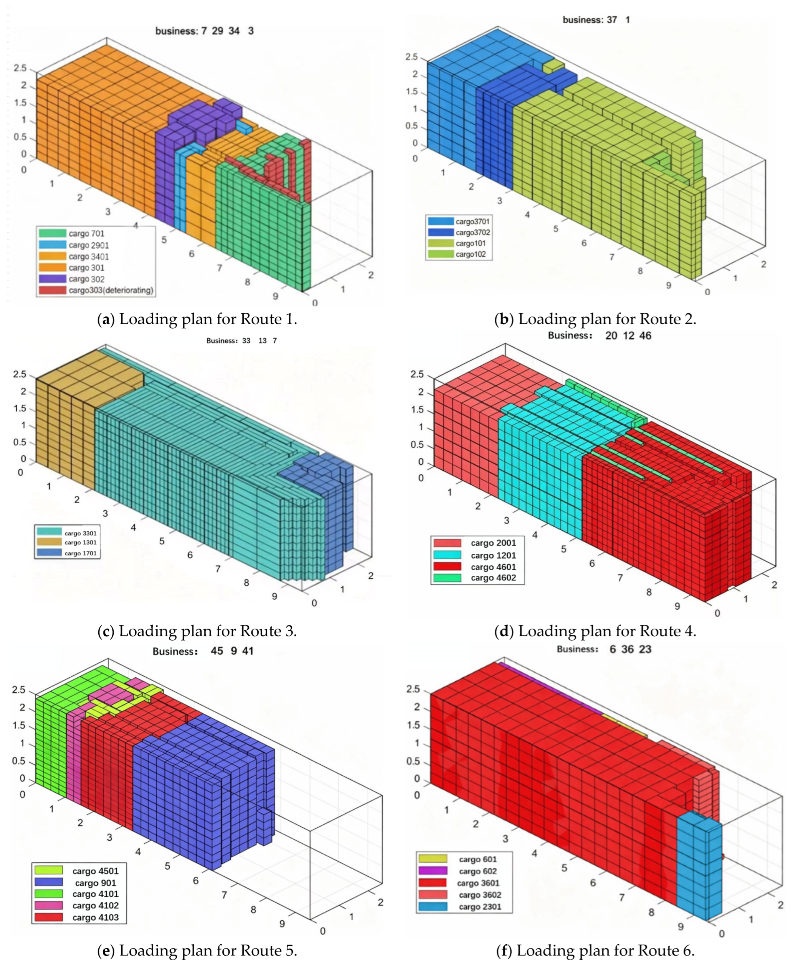
Agricultural products have diverse packaging sizes, and are highly vulnerable to contamination. In this study, stacking and support area constraints were added to the system in the collection path planning model, which is designed for the unique physical attributes of agricultural products. From the loading results, the average load utilization rate reached 90.20%, the average volume utilization rate was 72.20%, and the maximum load utilization rate was 99.58%. This shows that the algorithm can still achieve high space utilization when stacking constraints and support area requirements are considered. Although the model in this study increases the complexity of the solution space, it ensures the geometric feasibility of the cargo collection scheme and avoids the secondary scheduling costs caused by loading failure.

(3)

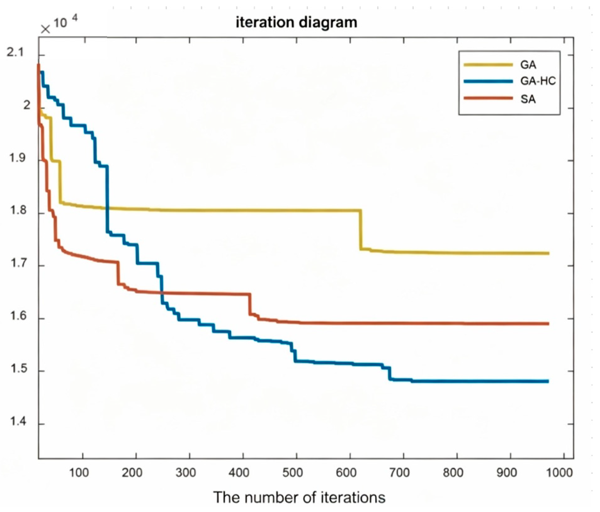
The genetic–hill-climbing adaptive hybrid algorithm designed in this study was improved in four aspects: greedy initialization, adaptive crossover and mutation, elite retention, and hill-climbing local search. Compared with the standard genetic algorithm, the hybrid algorithm reduced the total cost by 14.1%, reduced the number of paths from 23 to 20, and increased the average load utilization rate from 78.43% to 90.20%. Compared with the simulated annealing algorithm, the total cost was reduced by 6.8%, and the convergence speed was moderate. The advantages of the hybrid algorithm are as follows: greedy initialization provides a high-quality starting point for the population, and adaptive crossover and mutation maintain diversity in the early stages of evolution, and convergence in the later stages. The introduction of a hill-climbing operator effectively alleviates the problem that genetic algorithm is easily falling into the local optimum.

(4)

Under the framework of carbon tax policy, this study converts carbon emissions into cost items into an objective function. The results show that the carbon emission cost of the hybrid algorithm is 348.5 yuan, which is 5.5% lower than that of the genetic algorithm (369 yuan) and 7.4% lower than that of simulated annealing (376.3 yuan). The reduction in carbon emissions is mainly due to two factors: path optimization reduces the total driving distance, and an increase in the load utilization rate reduces the fuel consumption of unit cargo transportation. This shows that economic and environmental goals do not conflict in this model but achieve collaborative optimization by improving resource utilization.

(5)

The inventory replenishment rule used in this study is a simple heuristic (replenish up to the forecast when stock falls below the safety level). Its performance in terms of stockout rates, overstock rates, or forecast error sensitivity has not been evaluated. Therefore, no conclusion is drawn about reductions in warehousing costs or lost sales. This rule should be interpreted only as a trigger for collection operations, not as an optimized inventory-management policy.

(6)

The support area constraint only compares the length, width, and base area of items; it does not model the actual contact overlap or the alignment with the center of gravity. Therefore, the loading feasibility assessed in this study is geometric, not physical. The absence of explicit center-of-gravity calculation further limits the practical safety of the proposed loading plans, especially for heavy agricultural products such as rice sacks and oil drums. Future work should incorporate axle load constraints and dynamic stability checks.

In summary, the proposed method achieves significant improvements across the three dimensions of sustainability: at the economic level, total cost is reduced by 14.1%; at the environmental level, carbon emissions are reduced by 5.5%; and at the operational level, the average load utilization rate is increased to 90.20%. These outcomes not only align with the development goals of green logistics but also offer a feasible paradigmatic basis for the sustainable transformation of similar agricultural logistics systems.

This study has the following limitations:

(1)

Sales forecasting is based only on historical time series and does not include external factors such as weather, holiday promotions, or market prices, which may affect the capture accuracy of demand fluctuations.

(2)

Vehicle routing planning assumes that all requirements are known and static, without considering dynamic changes in real-time order insertion or traffic congestion.

(3)

The three-dimensional loading algorithm assumes that the items are all regular cuboids, and only 90° rotation is allowed, which has limited adaptability to special-shaped packaging or flexible packaging agricultural products.

(4)

All vehicles are diesel vehicles, and new energy transportation modes such as electric vehicles have not been explored.

Based on these limitations, future research can be conducted in the following directions.

(1)

A multivariate prediction model is introduced to further improve the accuracy of sales forecasting.

(2)

Explore the path-charging joint optimization model of electric vehicles to further reduce carbon emissions.

(3)

The three-dimensional loading algorithm was extended to support irregular cargo shapes and more flexible rotations.

Additionally, the absence of explicit center-of-gravity calculation is a simplification that may affect feasibility for very heavy or unbalanced loads; future work should incorporate axle load constraints.

5.2. Managerial and Policy Implications

5.2.1. Managerial Implications

The findings of this study offer several actionable insights for managers of agricultural cloud warehouses and e-commerce logistics operators. First, demand-driven collection reduces waste. By using sales forecasting to trigger replenishment instead of fixed-interval collection, managers can align vehicle dispatch with actual inventory needs. In our case study, this approach achieved an average load utilization of 90.20%, implying that nearly all vehicle capacity is used, which reduces the number of trips and lowers per-unit transportation cost. Second, fragility-aware loading is an opportunity, not a constraint. Many logistics managers avoid stacking fragile items altogether, leading to low space utilization. Our stacking and merging rules allow safe stacking of non-fragile items below fragile ones, increasing volume utilization from typical 50–60% to 72.20% in our experiments. Third, hybrid algorithms justify the computational investment. While simpler heuristics (e.g., simulated annealing) converge faster, the proposed hybrid algorithm reduces total cost by 6.8% and carbon emissions by 7.3% compared to SA. For a warehouse dispatching 20 routes per month, this translates into annual savings of approximately 12,100 CNY in direct costs, not including carbon tax savings. Fourth, sensitivity to forecasting errors is manageable. Even with ±10% forecasting error, total cost increases by only 3.88% and the number of routes remains stable. This suggests that investing in highly sophisticated forecasting (e.g., incorporating real-time promotion data) may yield diminishing returns; a robust hybrid model with 10–15% MAPE is practically sufficient.

5.2.2. Policy Implications

From a policy perspective, this study provides evidence for several regulatory and strategic directions. Carbon tax internalization works: By converting carbon emissions into a cost term, the model naturally reduces emissions (5.5% in our case) without sacrificing economic performance. Policymakers can consider expanding carbon pricing mechanisms to agricultural logistics, as the economic penalty creates direct incentives for green routing and loading. Support for smart agricultural logistics infrastructure: The integration of cloud warehouse management systems with forecasting and routing algorithms requires investment in data sharing platforms. Governments could subsidize the adoption of such integrated systems for small and medium-sized agricultural e-commerce players, because the social benefits (reduced emissions, less road congestion from empty runs) accrue beyond private gains. Seasonal demand data as a public good: Our STL decomposition revealed clear seasonal patterns for rice, maize, alcohol, dried items, and instant beverages. Agricultural statistical agencies could publish regional seasonal demand indices to help smaller warehouses without extensive historical data benefit from similar optimization. Encouraging fragile-friendly packaging standards: The stacking constraints in our model highlight that package dimensions and fragility labeling are critical for 3D loading efficiency. Policymakers could promote voluntary packaging standards (e.g., maximum stack height, weight-bearing capacity labels) to facilitate automated loading optimization across different logistics providers.

5.3. Sensitivity Analysis of the Empty-Run Penalty Coefficient

The empty-run penalty coefficient ε₁ in Equation (8) directly affects the trade-off between load utilization and total cost. To evaluate its influence, we tested three values: ε₁ = 20 (low penalty), ε₁ = 200 (baseline value used in this study), and ε₁ = 2000 (high penalty). All other parameters were kept identical. The experiment was conducted on the same instance with 48 merchants, and each setting was run 30 times.

Table 11. Sensitivity analysis of the empty-run penalty coefficient ε₁.

ε1	Number of Routes	Average Load Utilization (%)	Fixed Cost (CNY)	Fuel Cost (CNY)	Carbon Cost (CNY)	Empty-Run Penalty (CNY)	Total Cost (CNY)	Avg. Route Length (km)
20	22	85.30 ± 1.80	11,000	2950	370	502.5	14,822.50 ± 201.9	82.0
200	20	90.20 ± 1.50	10,000	2777	348	1129.4	14,254.40 ± 139.7	78.5
2000	19	92.10 ± 1.40	9500	2650	338	1561.6	14,043.60 ± 132.6	76.2

summarizes the average results.

As ε₁ increases, the model imposes a higher penalty on underutilized vehicles, which encourages fuller loading and reduces the number of routes from 22 (ε₁ = 20) to 19 (ε₁ = 2000). However, the empty-run penalty itself increases sharply from 502.5 CNY to 1561.6 CNY, and the average route length shortens only slightly. While ε₁ = 2000 yields the lowest total cost (14,043.6 CNY) and the highest load utilization (92.10%), the improvement over ε₁ = 200 is only about 210 CNY (less than 1.5%). Moreover, the operating plan with ε₁ = 2000 results in a much higher empty-run penalty (1561.6 vs. 1129.4 CNY) and a marginal reduction in average route length (76.2 vs. 78.5 km), indicating that the additional penalty forces the algorithm to eliminate a route at the cost of over-penalizing the remaining routes. In contrast, ε₁ = 200 provides a balanced solution: it uses a moderate number of routes (20), achieves 90.20% load utilization, and keeps the empty-run penalty at a reasonable level. Therefore, ε₁ = 200 is selected as the baseline for this study, as it represents the “elbow point” where further increase in ε₁ yields diminishing returns. The sensitivity analysis confirms that the main conclusions (e.g., the hybrid algorithm’s superiority) are robust within a reasonable range of ε₁ (20 to 2000).

6. Conclusions

To address the problems of low pickup efficiency, low load utilization rate, and high carbon emissions in the traditional special vehicle collection mode of cloud warehouses for agricultural products, this study proposed a collection path planning method based on sales forecasts. The main conclusions are as follows.

(1)

In terms of sales forecasting, seasonal differences in agricultural product sales were identified using STL decomposition, and a SARIMA/ARIMA-BPNN combined forecasting model was constructed. Experiments showed that the MAPE of the combined model for seasonal items was as low as 3.50%, which was approximately 15% lower than that of the single model, and provided a reliable demand input for collection path planning.

(2)

With respect to model construction, with the goal of minimizing vehicle fixed cost, fuel consumption cost, and carbon emission cost and maximizing the load utilization rate, a three-dimensional loading and collection path planning model considering stacking constraints and support area constraints was established, which makes the model more suitable for the actual transportation demand of agricultural product vulnerability.

(3)

In the aspect of algorithm solution, a two-stage solution framework of ‘path planning–loading test’ is designed. In the path planning stage, an improved genetic–hill-climbing adaptive hybrid algorithm (greedy initialization, adaptive crossover and mutation, and elite retention) is adopted. In the loading test stage, a constructive heuristic algorithm based on ‘stack’ dimension reduction and the lower left–best adaptation fusion rule is developed.

(4)

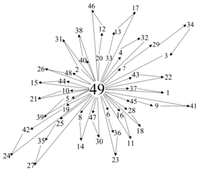
In terms of empirical verification, taking the real data of 48 agricultural product merchants in Harbin as an example, the proposed method achieved an average load utilization rate of 90.20% and an average volume utilization rate of 72.20% on 20 collection routes. Compared with the genetic algorithm and simulated annealing algorithms, the total cost is reduced by 14.1% and 6.8%, respectively, and the carbon emission cost is reduced by more than 5.5%.

(5)

From a sustainability perspective, the proposed method demonstrates significant improvements across the three core dimensions. Economically, the total cost reduction of 14.1% lowers the operational expenses of cloud warehouses. Environmentally, the 5.5% reduction in carbon emissions directly contributes to green logistics and climate change mitigation. Operationally, the average load utilization rate of 90.20% implies a more efficient use of vehicle capacity, reducing empty-run costs by 36.8% and minimizing resource waste. These results confirm that the integrated optimization of sales forecasting, three-dimensional loading constraints, and routing decisions can simultaneously enhance economic viability, environmental performance, and operational efficiency.

This study provides a sustainable development path for cloud warehouses of agricultural products to improve collection efficiency and reduce operating costs and carbon emissions. In the future, multivariate prediction models will be introduced and dynamic scheduling mechanisms will be explored.

References

- Chen, Y.; Xie, X.; Pei, Z. Development of a time series e-commerce sales prediction method for short-shelf-life products using GRU-LightGBM. Appl. Sci. 2024, 14, 866. [Google Scholar] [CrossRef] [Scilit]
- Xie, L.; Liu, J.Q.; Wang, W. Predicting sales and cross-border e-commerce supply chain management using artificial neural networks and the Capuchin search algorithm. Sci. Rep. 2024, 14, 13297. [Google Scholar] [CrossRef] [Scilit] [PubMed]
- Yuan, R.P.; Wei, H.; Fu, Z.J. Research on e-commerce enterprise product sales forecasting integrating CNN and WDF models. Comput. Eng. Appl. 2025, 61, 335–343. [Google Scholar]
- Avinash, G.; Ramasubramanian, V.; Ray, M.; Paul, R.K.; Godara, S.; Nayak, G.H.; Kumar, R.R.; Manjunatha, B.; Dahiya, S.; Iquebal, M.A. Hidden Markov guided deep learning models for forecasting highly volatile agricultural commodity prices. Appl. Soft Comput. 2024, 158, 111557. [Google Scholar] [CrossRef] [Scilit]
- Mu, S.D.; Wang, Y.Y.; Wang, F.Y.; Ogiela, L. Transformative computing for products sales forecast based on SCIM. Appl. Soft Comput. 2021, 109, 107520. [Google Scholar] [CrossRef] [Scilit]
- Ibáñez, S.C.; Monterola, C.P. A global forecasting approach to large-scale crop production prediction with time series transformers. Agriculture 2023, 13, 1855. [Google Scholar] [CrossRef] [Scilit]
- Li, H. Demand forecast of cold chain logistics of fresh agricultural products based on deep learning. In Proceedings of the 2024 International Conference on Industrial IoT, Big Data and Supply Chain (IIoTBDSC), Wuhan, China, 22 September 2024; pp. 296–300. [Google Scholar]
- Xu, X.-F.; Yu, L.; Lin, Z.-R.; Sun, Y. Short-term sales ensemble forecasting of fresh products based on feature fusion. J. Manag. Sci. 2022, 25, 102–123. [Google Scholar]
- Chaabane, A.; Montecinos, J.; Ouhimmou, M.; Khabou, A. Vehicle routing problem for reverse logistics of End-of-Life Vehicles (ELVs). Waste Manag. 2021, 120, 209–220. [Google Scholar] [CrossRef] [Scilit] [PubMed]
- Ren, Y.; Lu, X.; Guo, H.; Xie, Z.; Zhang, H.; Zhang, C. A review of combinatorial optimization problems in reverse logistics and remanufacturing for end-of-life products. Mathematics 2023, 11, 298. [Google Scholar]
- Gao, Z.; Ye, C. Reverse logistics vehicle routing optimization problem based on multivehicle recycling. Math. Probl. Eng. 2021, 2021, 5559684. [Google Scholar] [CrossRef] [Scilit]
- Zhang, M.J.; Prataps, S.; Zhao, Z.H.; Prajapati, D.; Huang, G.Q. Forward and reverse logistics vehicle routing problems with time horizons in B2C e-commerce logistics. Int. J. Prod. Res. 2021, 59, 6291–6310. [Google Scholar] [CrossRef] [Scilit]
- Marseglia, G.; Mesa, J.; Ortega, F.; Piedra-De-La-Cuadra, R. A heuristic for the deployment of collecting routes for urban recycle stations (eco-points). Socio-Econ. Plan. Sci. 2022, 82, 101222. [Google Scholar] [CrossRef] [Scilit]
- Golman, R.; Mohammadi, M.; Hajiaghaki, K.M.; Fusco, G.; Colombaroni, C. An integrated temporal and spatial synchronization for two-echelon vehicle routing problem in waste collection system. J. Ind. Inf. Integr. 2024, 40, 100611. [Google Scholar] [CrossRef] [Scilit]
- Min, L.Y.; Shin, F.Y. Solving the green reverse logistics problem in e-commerce using a reinforcement learning based genetic algorithm. Electron. Commer. Res. Appl. 2024, 68, 10145. [Google Scholar] [CrossRef] [Scilit]
- Wang, Y.J.; Luo, S.; Fan, J.; Zhen, L. The multidepot vehicle routing problem with intelligent recycling prices and transportation resource sharing. Transp. Res. Part E Logist. Transp. Rev. 2024, 185, 103503. [Google Scholar] [CrossRef] [Scilit]
- Roy, A.; Manna, A.; Kim, J.; Moon, I. IoT-based smart bin allocation and vehicle routing in solid waste management: A case study in South Korea. Comput. Ind. Eng. 2022, 171, 108457. [Google Scholar] [CrossRef] [Scilit]
- Cao, S.; Liao, W.W.; Huang, Y. Heterogeneous fleet recyclables collection routing optimization in a two-echelon collaborative reverse logistics network from circular economic and environmental perspective. Sci. Total Environ. 2021, 758, 144062. [Google Scholar] [CrossRef] [Scilit] [PubMed]
- Zhuo, B.W.; Wen, M. A multi-objective artificial electric field algorithm with reinforcement learning for milk-run assembly line feeding and scheduling problem. Comput. Ind. Eng. 2024, 190, 110080. [Google Scholar] [CrossRef] [Scilit]
- Julian, B. Environmental aspects in supplier networks—A bi-objective just-in-time vehicle routing problem. Int. J. Prod. Res. 2024, 62, 4290–4313. [Google Scholar] [CrossRef] [Scilit]
- Xu, R.T.; Huang, Y.; Xiao, W. A two-level variable neighborhood descent for a split delivery clustered vehicle routing problem with soft cluster conflicts and customer-related costs. Sustainability 2023, 15, 7639. [Google Scholar]
- Polat, O.; Topaloglu, D. Collection of different types of milk with multi-tank tankers under uncertainty: A real case study. Top 2022, 30, 1–33. [Google Scholar]
- Quan, C.; He, Q.B.; Ye, X.; Cheng, X. Optimization of the milk-run route for inbound logistics of auto parts under low-carbon economy. J. Algorithms Comput. Technol. 2021, 15, 17483. [Google Scholar] [CrossRef] [Scilit]
- Xu, W.; Li, B.; Cui, W.Z.; Li, R.; Du, X.; Xing, L. A greedy tabu dual heuristic algorithm for the cyclic pickup and delivery problem with 3D loading constraints. Sci. Rep. 2024, 14, 31762. [Google Scholar] [CrossRef] [Scilit] [PubMed]
- Zhou, B.T.; Zhao, Z. An adaptive artificial bee colony algorithm enhanced by deep Q-learning for milk-run vehicle scheduling problem based on supply hub. Knowl.-Based Syst. 2023, 264, 110367. [Google Scholar] [CrossRef] [Scilit]
- Zhang, Q.Q.; Chen, Q. Improved decentralized search algorithm for solving packaging waste recycling path planning problems. Packag. Eng. 2024, 45, 193–200. [Google Scholar]
- Thanh, N.H.; Nguyen, X.T. Space splitting and merging technique for online 3-D bin packing. Mathematics 2023, 11, 1912. [Google Scholar] [CrossRef] [Scilit]
- Zhu, W.; Chen, S.; Dai, M.M.; Tao, J. Solving a 3D bin packing problem with stacking constraints. Comput. Ind. Eng. 2024, 188, 109814. [Google Scholar]
- Youssef, H. A three-stage layer-based heuristic to solve the 3D bin-packing problem under balancing constraint. J. King Saud Univ. Comput. Inf. Sci. 2022, 34, 6425–6431. [Google Scholar]
- Tu, C.; Tai, J.-Y.; Vu, T.-L.; Chen, T.-H. Multiple bin-size bin packing problem considering incompatible product categories. Expert Syst. Appl. 2024, 247, 123340. [Google Scholar] [CrossRef] [Scilit]
- Hoa, N.T.X. Optimizing container fill rates for the textile and garment industry using a 3D bin packing approach. HighTech Innov. J. 2024, 5, 462–478. [Google Scholar] [CrossRef] [Scilit]
- Hamid, S.H.; Kashan, H.; Ostabi, B. A three-dimensional bin packing problem with item fragmentation and its application in the storage location assignment problem. 4OR 2024, 22, 483–536. [Google Scholar] [CrossRef] [Scilit]
- Jonas, H.; Erik, J.; Gyözö, G.; Cats, O. Modular vehicle routing for combined passenger and freight transport. Transp. Res. Part A Policy Pract. 2023, 173, 103688. [Google Scholar] [CrossRef] [Scilit]
- Ana, N.A.A.; Ribero, L. A multi-heuristic algorithm for multi-container 3-d bin packing problem optimization using real world constraints. IEEE Access 2024, 12, 42105–42130. [Google Scholar]
- Liu, Y.; Jiang, X. Dynamic feedback algorithm based on spatial corner fitness for solving the three-dimensional multiple bin-size bin packing problem. Complex Intell. Syst. 2024, 10, 4055–4081. [Google Scholar] [CrossRef] [Scilit]
- Yang, J.X.; Liu, H.; Liang, K.; Zhou, L.; Zhao, J. Variable neighborhood genetic algorithm for multi-order multi-bin open packing optimization. Appl. Soft Comput. 2024, 163, 111890. [Google Scholar] [CrossRef] [Scilit]
- Jia, K. Research on optimization of three-dimensional loading problem based on genetic algorithm. Meas. Test. Technol. 2023, 50, 75–78. [Google Scholar]
- Qi, M.; Zhang, L. Online 3D packing problem based on bi-value guidance. J. Comput. Commun. 2023, 11, 31–45. [Google Scholar] [CrossRef]
- Zhou, L.; Yang, J.L.; Zhao, J.H.; Liu, H.; Wang, F. Research on multi-box three-dimensional loading problem based on hybrid genetic algorithm. Packag. Eng. 2022, 43, 213–223. [Google Scholar]
- Amalana, S.M.; Jumyung, U. BoxStacker: Deep reinforcement learning for 3D bin packing problem in virtual environment of logistics systems. Sensors 2023, 23, 6928. [Google Scholar] [CrossRef] [Scilit] [PubMed]