Integrating Reddening Phenology of Suaeda salsa for Sustainable Sentinel-2-Based Classification of Coastal Wetland Vegetation in Jiangsu Province

Abstract

Protecting native coastal wetland vegetation and controlling the invasion of Spartina alterniflora (SA) have long been key ecological and management priorities in China. The accurate and rapid mapping of vegetation distribution is critical for effective invasion control and wetland restoration. While phenological information improves remote sensing classification, most studies rely on the Normalized Difference Vegetation Index (NDVI), which has limited capability to distinguish morphologically similar species in coastal wetlands. To better exploit the unique reddening phenology of one such species, Suaeda salsa (SS), this study builds on our previously developed Red Suaeda salsa Index (RSSI) and introduces two novel phenological indicators: the Redness Contribution Coefficient (RCC) and Reddening Rate Index (RCI). Using the coastal wetlands of Jiangsu Province as the study area, we employed multi-temporal Sentinel-2 image composites (spring, summer, autumn) from 2019, 2022, 2024, and 2025 to construct a multi-dimensional feature set and implemented classification using a random forest algorithm. Results showed that the feature scheme integrating SS reddening phenological parameters achieved the highest accuracy, with an overall accuracy of 97.32% and a Kappa coefficient of 0.9625 in 2019, confirming the method’s reliability at the provincial scale. Between 2019 and 2025, SA coverage in Jiangsu decreased by 90.8%, with most cleared areas converting to non-vegetated land, indicating the remarkable effectiveness of recent control projects. This study scales up a locally validated high-precision classification approach to the provincial scale, supporting sustainable coastal wetland management in line with United Nations (UN) SDG 14 (Life Below Water) and SDG 15 (Life on Land).

1. Introduction

Coastal wetlands provide critical ecosystem services, including shoreline stabilization, water purification, and biodiversity conservation [1]. These functions are fundamental to achieving the UN Sustainable Development Goals (SDGs), especially SDG 14 (Life Below Water) and SDG 15 (Life on Land). While coastal wetlands underpin regional ecological security, they are increasingly threatened by invasive plant species. For instance, Spartina species have caused widespread wetland degradation across Europe and North America and impaired wetland sustainability.

Introduced to China in 1979 for coastal erosion control, Spartina alterniflora (SA) has become a notorious invasive species. It has occupied more than 17,800 hm² of coastal wetlands in Jiangsu Province [2,3], outcompeting native Phragmites australis (PA) and Suaeda salsa (SS) for light, water, and nutrients. SA alters the surface elevation, light availability and soil salinity, resulting in habitat loss for waterbirds and native plants. Such changes greatly hinder sustainable wetland management and progress toward SDG targets. To address this issue, China launched a national action plan for SA control (2022–2025) [4], with Jiangsu designated as a key priority region. This effort is further strengthened by the coastal spatial planning issued by the Jiangsu Provincial Government [5]. Reliable vegetation monitoring is therefore essential for evaluating control outcomes and guiding ecological restoration.

Remote sensing has been widely applied to wetland vegetation mapping [6,7,8]. Nevertheless, the accurate classification of SA, PA, and SS remains difficult due to spectral similarity, frequent tidal inundation, and strong spatial heterogeneity. Although machine learning and deep learning approaches have been adopted, they usually require massive training datasets and still struggle with fine-scale species discrimination [9,10,11]. By contrast, interspecific phenological differences offer a promising alternative [12]: SA presents an earlier green-up and later senescence [13], while SS exhibits a unique autumn reddening phenology [14]. Such phenological differences can be used for species classification [15,16]. Most existing phenology-based studies rely on NDVI, which is insensitive to distinct phenological traits, especially the autumn reddening of SS. Benefiting from a 5-day revisit interval and red-edge bands, Sentinel-2 can capture subtle spectral variations during phenological transitions (e.g., green-up, senescence, and reddening) and is thus highly suitable for monitoring such processes [17].

Several species-specific spectral indices including SSVI and SSSI have been developed for SS monitoring [18,19], yet they show poor cross-region transferability and have only been validated in relatively homogeneous sites. Our previous study proposed the Red Suaeda salsa Index (RSSI) and RSSI1 based on shortwave infrared (SWIR) reflectance [20]. SWIR reflectance rises during SS reddening due to cell wall degradation and pigment variation, and the proposed indices improved classification accuracy by over 15% at local sites in Lianyungang. Despite satisfactory local performance, this method cannot be directly extended to the provincial scale due to three major constraints: (1) phenological asynchrony along latitudinal gradients, (2) spectral disturbance caused by tidal inundation, and (3) the necessity of seasonal composites to characterize phenological variability. Solving these problems will help maintain long-term coastal ecosystem sustainability and advance the implementation of SDG 14 and 15.

Against the above research gaps, this study sets two main objectives. First, we aim to verify whether two newly proposed phenological parameters targeting SS reddening—the Redness Contribution Coefficient (RCC) and Reddening Rate Index (RCI)—can outperform traditional NDVI- and RSSI-based methods in classification accuracy. Second, we evaluate the transferability of the locally-derived method by applying it to the entire Jiangsu Province, which encompasses three representative coastal regions (Lianyungang, Yancheng, and Nantong) with divergent tidal and phenological conditions. In this work, we extend the RSSI-based approach to the provincial scale, integrate RCC and RCI, and adopt seasonal composite images (spring, summer, and autumn) to stabilize phenological signal extraction. Using multi-temporal Sentinel-2 imagery acquired from 2019 to 2025, we classify SA, PA, and SS and map the spatial patterns of SA control effectiveness across Jiangsu coastal wetlands. The outcomes of this study can provide a robust technical framework for large-scale wetland vegetation monitoring, support invasive species management and native ecosystem restoration, and contribute to national and global sustainable development agendas (SDGs).

2. Materials and Methods

2.1. Study Area

The coastal wetlands of Jiangsu Province (31°59′–35°07′ N, 118°24′–122°03′ E) are located in the middle section of the eastern coast of China, covering the cities of Lianyungang, Yancheng, and Nantong (Figure 1: Study area, with the base map presented in composite standard false color for autumn 2022). Many of the major wetlands are listed in the List of Important Terrestrial Wildlife Habitats [21] and play an important role in biodiversity conservation in China and globally. The region has a monsoon climate that transitions from subtropical to warm temperate, with mild, humid conditions and abundant rainfall. The combination of silty mudflats and saline–alkali wetland soils provides a unique habitat for salt-tolerant wetland vegetation and has become the main distribution area of Spartina alterniflora (SA). Introduced in the 1970s, SA once played a positive role in protecting beaches and dikes and promoting siltation and land reclamation. However, its unchecked expansion has displaced native vegetation, posing a serious threat to regional ecological security. In the Ganyu, Linhong, and Liezi estuarine wetlands of Lianyungang, SA invasion has impaired ecological functions and reduced the quality of key stopover sites for migratory birds [22]. The Jiangsu Yancheng Wetlands and Rare Birds National Nature Reserve is a key habitat for more than 60% of the global wintering population of red-crowned cranes. Here, the expansion of SA has severely displaced native vegetation such as PA and SS (

Table 1. Vegetation types and distribution characteristics of the study area.

Vegetation Type	Image	Spatial Distribution Characteristics	Field Visit Photos
PA		Perennial Poaceae grass forming reed marshes in river mouths and wetlands.
SS		Annual Chenopodiaceae herb adapted to high-salt habitats.
SA		Perennial salt-tolerant Poaceae grass, clump-growing in coastal tidal zones.

). The Xiaoyangkou coastal wetlands in Rudong County are located in the Yellow Sea radiating sandbar zone of Nantong City. The spread of SA has impacted the vegetation community structure of silty mudflats, making it a key area for regional ecological governance. This study takes a 2 km buffer zone along the coastline of Jiangsu Province, together with the aforementioned typical wetlands, as the study area. It extracts coastal wetland vegetation from 2019 to 2025 and analyzes its dynamics.

2.2. Dataset

2.2.1. Image Data

The research data were obtained through the Google Earth Engine (GEE) cloud platform [23], using the Sentinel-2 L2A surface reflectance product (data ID: COPERNICUS/S2_SR) [24] that had undergone preprocessing such as atmospheric correction. The projection system used was UTM50N/WGS1984. The study selected annual images from 2019, 2022, 2024, and 2025 with cloud cover less than 20% (Figure 2). For each target year, images were grouped into three seasonal composites: spring (April–May), summer (June–August), and autumn (September–November). The number of valid observations per season and per year is shown in Figure 2, with generally consistent scene counts across years and seasons (approximately 20–40 scenes in spring, 40–60 in summer, and 30–50 in autumn), ensuring balanced seasonal coverage for phenological analysis. Cloud removal (based on the QA60 quality control band) and median composition were then performed for each seasonal composite.

Regarding tidal influence, tidal height data were not used as a direct filtering criterion for image selection. Instead, the median composite over multiple observations within each seasonal window inherently reduces the spectral bias caused by transient tidal inundation, as tidal levels vary across acquisition dates. For pixels that are occasionally submerged, the median operation selects the most frequently occurring reflectance values, which correspond to exposed conditions during low-to-mid tides. This approach follows established practices for intertidal wetland mapping.

2.2.2. Sample Selection

This experiment employed a combination of the Global Navigation Satellite System (GNSS) and unmanned aerial vehicles (UAVs) to precisely locate the distribution of vegetation samples. High-resolution UAV photography acquired detailed field imagery data, effectively capturing the spatial distribution of vegetation. Based on existing coastal wetland classifications and visual interpretation (

Table 2. Sample selection method (taking Linhong Estuary Wetland as an example).

Photo Sampling	UAV Photography	Visual Interpretation

), the wetlands in the study area were divided into four categories: Phragmites australis (PA), Suaeda salsa (SS), Spartina alterniflora (SA), and Non-vegetated Area (NA). Sample collection was conducted independently for each target year (2019, 2022, 2024, and 2025). For 2019 and 2022, samples were obtained through visual interpretation of high-resolution time-series imagery (Google Earth historical imagery) combined with reference to existing published studies [25]. Specifically, seasonal composite images (spring, summer, autumn) for each target year were examined: spring images captured the start of the growing season, summer images captured peak growth characteristics, while autumn images captured the reddening signature of SS, which helped distinguish SS from SA and PA. Cross-validation with published vegetation maps was also performed. For 2024 and 2025, five field campaigns were conducted (November 2024; March, May, July, and November 2025) after obtaining permission from the relevant authorities. These campaigns integrated UAV surveys, GNSS positioning, and ground observations to collect samples. Each field campaign produced an independent set of observations; surveys were not repeated at fixed points across different times. Therefore, no assumption of temporal constancy was made—classifications for different years were performed independently.

Figure 3 shows the spatial distribution of the 2019 samples (gray: training, pink: validation) as a representative example. A total of 4279 samples were collected for 2019, with class totals of 1278 for SA, 1182 for SS, 1179 for PA, and 640 for NA. The sample distributions for 2022, 2024, and 2025 followed a similar pattern to 2019 and are available from the authors upon request. For each target year, the samples were randomly split into training (70%) and validation (30%) sets based on a random number assignment, with class proportions balanced between the two subsets. Approximately 70% of the samples were used for training and for assessing phenological characteristics and spectral separability of SS from other vegetation. The remaining 30% were used for independent accuracy validation, ensuring representativeness of sample distribution and model generalizability.

Regarding inter-annual spectral variability, coastal wetland vegetation exhibits obvious interannual spectral discrepancies driven by changing climate and tidal regimes, as well as varied phenological rhythms. Moreover, phenological metrics were extracted independently for each year to match annual vegetation growth cycles. Accordingly, Random Forest models were separately retrained for 2019, 2022, 2024, and 2025 with year-specific training samples. No cross-year validation was conducted, and 2024–2025 samples were not used to validate earlier classification results. Each annual model was validated solely by its own 30% independent sample subset. This year-by-year modeling framework effectively accommodates inter-annual shifts in spectral and phenological features and enables each model to fit yearly field environments.

2.3. Methods

2.3.1. Remote Sensing Classification Feature Extraction

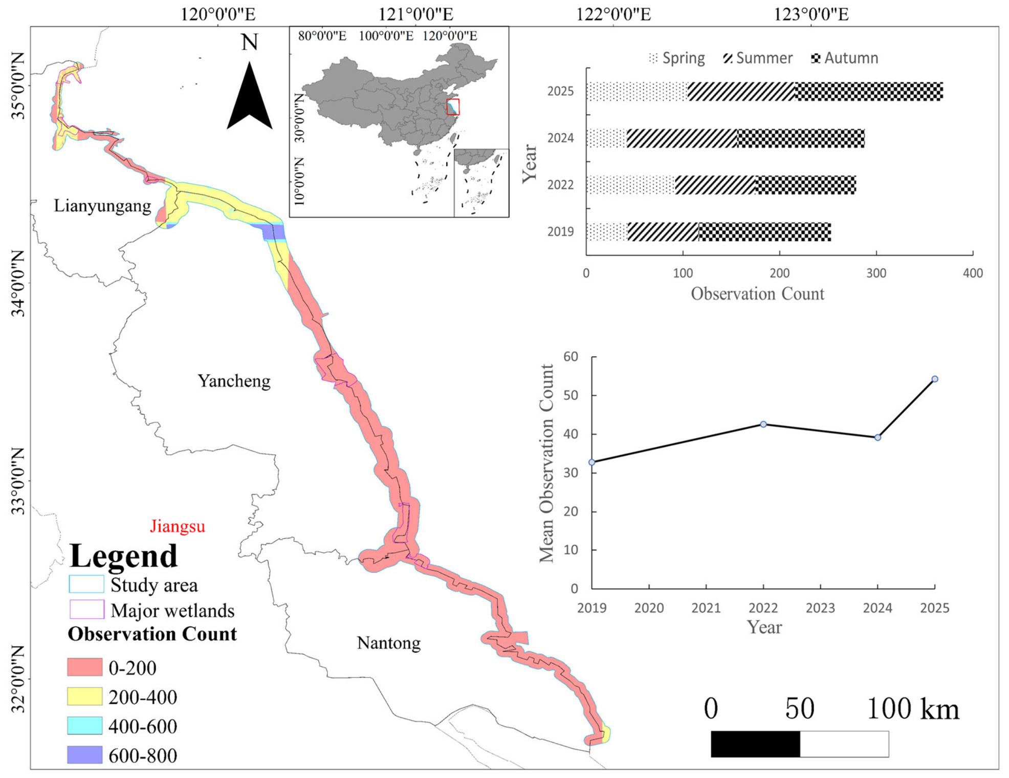
Phenological parameters were derived from the full time series of all available Sentinel-2 images (cloud cover < 20%) within each target year to preserve temporal continuity. Meanwhile, spectral indices, red-edge indices, and texture features were extracted from seasonal median composites (spring, summer, autumn) to ensure cloud-free and stable spatial features. The two sets of features were then integrated for classification.

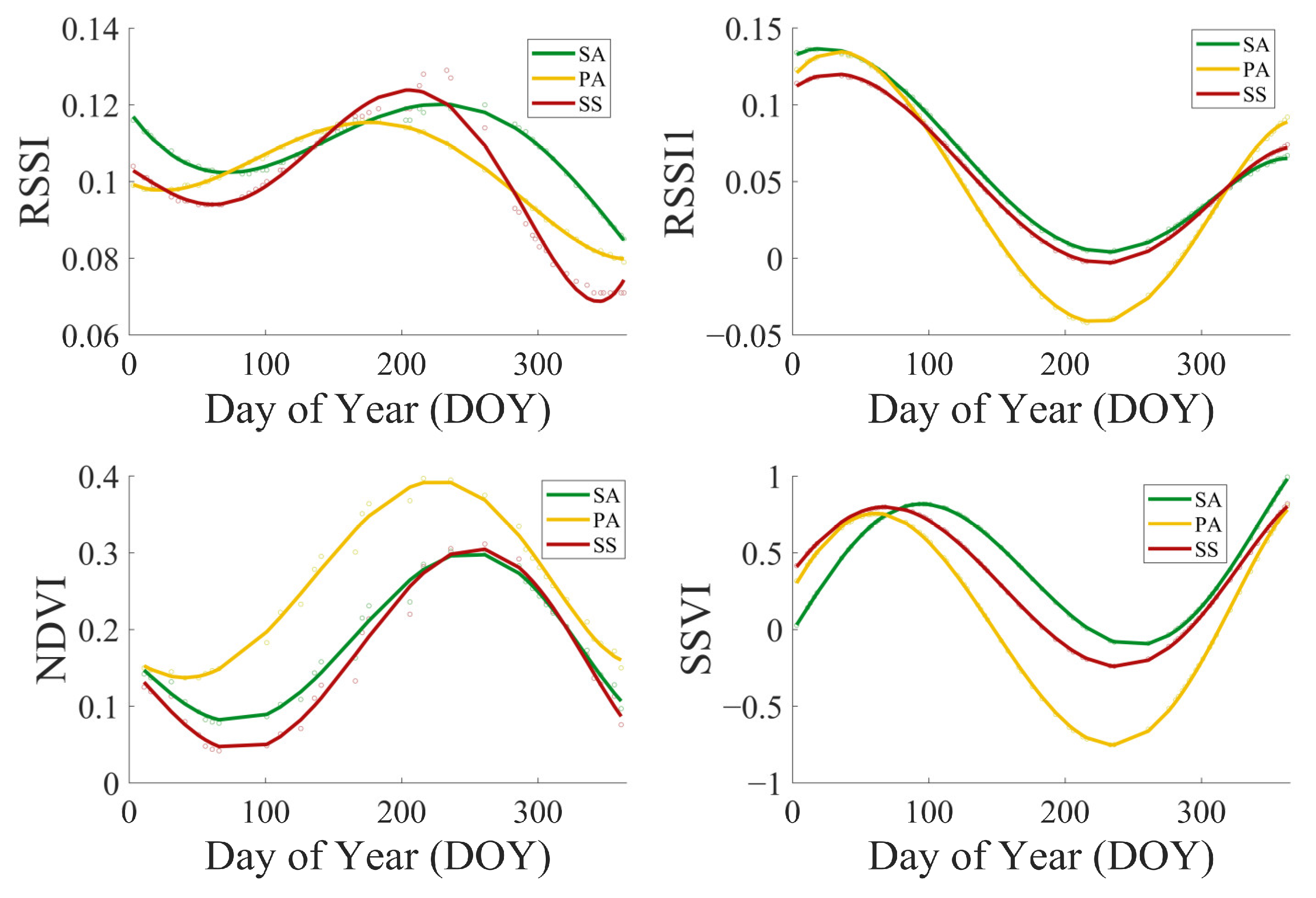
Based on Sentinel-2 images, phenological characteristics of coastal wetland vegetation were extracted following a four-step workflow. First, NDVI and SSVI were calculated for each acquisition date, generating a dense time series. Second, the raw time series were smoothed using the Savitzky-Golay (S-G) filter with a window size of 7 and polynomial order of 2, which preserves phenological trends while suppressing cloud and atmospheric noise. Third, the smoothed curves were fitted using a flexible Fourier function with one harmonic component combined with a linear trend term. This configuration is optimal for coastal salt marsh vegetation, accurately capturing their typical single-peak seasonal growth trajectories and producing continuous and reduced-noise phenological curves. Fourth, phenological parameters were extracted from the fitted curves: SOS (start of season) and EOS (end of season) were defined using a dynamic threshold set at 50% of the seasonal amplitude; BV (base value) and MV (maximum value) were extracted as the minimum and maximum of the fitted curve, respectively [26,27,28].

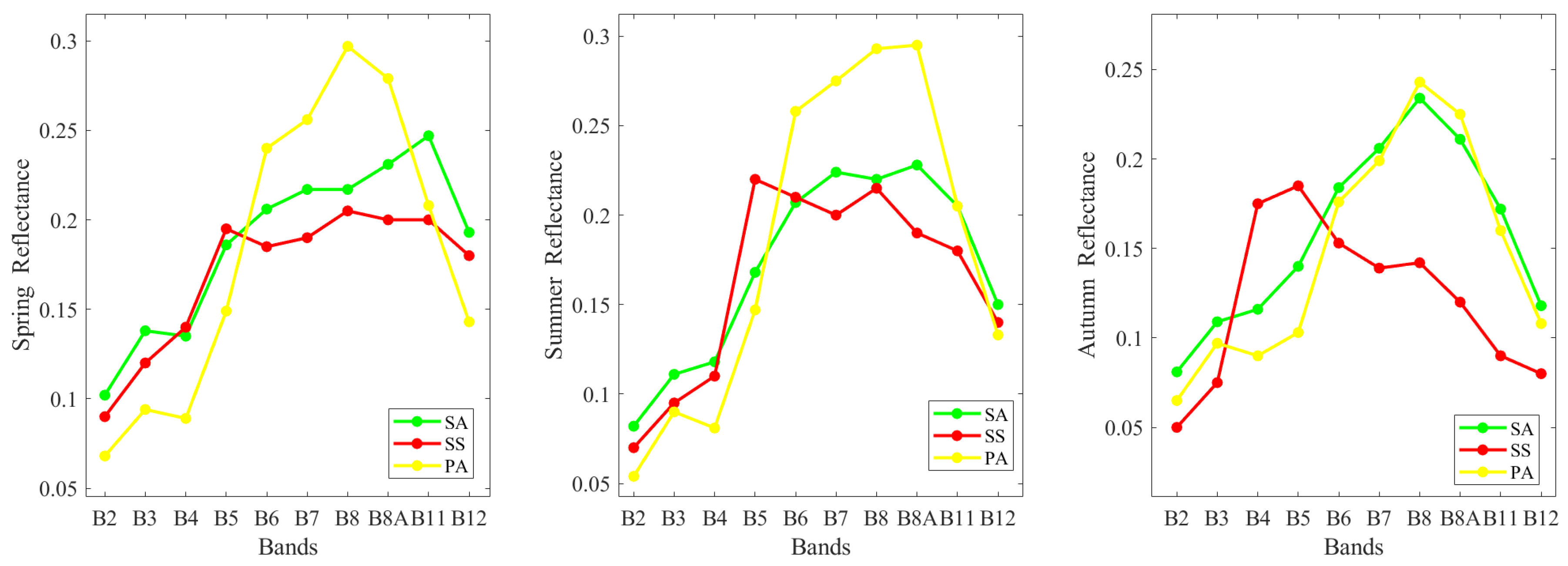
This study used median composite images of each season to generate the spectral reflectance of three vegetation types (Figure 4) to reduce the influence of cloud pollution and single-scene noise. These seasonal patterns were consistent with the conclusions of existing studies [29,30]: in spring, all three vegetation types were in the growth stage and the spectral differences were small; in summer, the near-infrared spectral reflectance of PA and SA reached its peak, SS began to redden, and the spectral characteristics shifted to the visible light band; in autumn, the reddening degree of SS reached its maximum, the reflectance of the visible light and short-wave infrared bands was enhanced, the near-infrared reflectance was reduced, and the spectral difference with the associated vegetation was further expanded. Based on this, the RSSI and RSSI1 were constructed. Their time series were processed following the identical workflow, including S-G smoothing (window size = 7, polynomial order = 2) and one-component Fourier harmonic fitting to ensure methodological consistency across all spectral indices. Since RSSI1 and SSVI phenological indicators were similar, conventional phenological parameters were also extracted (Figure 5). At the same time, based on the RSSI fitting curve, the window ratio method was used to extract the four SS indicators: Difference of RSSI (DOR), Sum of RSSI (SOR), Ratio of Green-up RSSI (ROSR), and Ratio of Senescence RSSI (ROGR) that the research team verified in Lianyungang City. The calculation formulas are shown in the Equations (1)–(6):

$$RSSI=\left({\displaystyle \frac{B2-B3}{B3-B4}}\right)\times \left({\displaystyle \frac{B4-B3}{B11}}\right)$$

(1)

$$RSSI1={\displaystyle \frac{B4-B3}{B11}}$$

(2)

$$DOR={RSSI}_{MV}-{RSSI}_{BV}$$

(3)

$$SOR={RSSI}_{MV}+{RSSI}_{BV}$$

(4)

$$ROSR={\displaystyle \frac{{RSSI}_{MV}}{RSSIsenescenc}}$$

(5)

$$ROGR={\displaystyle \frac{RSSIgreen-up}{{RSSI}_{BV}}}$$

(6)

In the Equations (1)–(6), the time windows and corresponding RSSI reference values are defined as follows: the base value time window refers to the initial stage of vegetation growth, generally corresponding to the valley of the phenology curve, used to define RSSI_BV; the green-up time window refers to the vegetation greening stage, used to define RSSIgreen − up; the maximum value time window refers to the vegetation maturity stage, generally corresponding to the peak of the phenology curve, used to define RSSI_MV; and the senescence time window refers to the vegetation senescence stage, used to define RSSIsenescence.

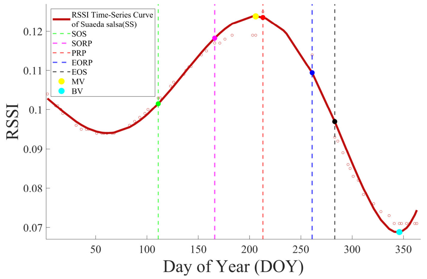
To better enhance the morphological differentiation ability of the SS reddening process, this study, based on the RSSI index, divided three types of time windows according to phenological key nodes (Figure 6):

• Full growing season window (SOS–EOS), corresponding to the complete growth cycle of vegetation;
• Reddening process window (Start of Reddening Period (SORP)–End of Reddening Period (EORP)), corresponding to the key stage from when the saltwort starts to turn red until the reddening is complete; SORP is defined as the date when RSSI reaches 70% of its peak amplitude. This threshold was empirically determined by testing values of 50%, 60%, 70%, 80%, and 90% of the peak RSSI amplitude on field-observed SS patches, where 70% best captured the onset of visible reddening. This threshold marks the initiation of rapid betalain synthesis and the associated increase in shortwave infrared reflectance, where the spectral contrast between SS, PA, and SA is maximized. EORP is defined as the date when RSSI drops to 50% of its peak after the maximum value (the end of reddening). The 50% threshold was selected because it consistently marked the end of the reddening phase in the fitted RSSI curves across all studied years and sites;
• Peak segmentation windows: SOS–Peak Reddening Period (PRP): The rising phase of the growing season, corresponding to the period from SOS to PRP; PRP–EOS: the falling phase of the growing season, corresponding to the period from PRP to EOS. The RSSI maximum value (MV) occurs at the left part of the peak plateau, while PRP is defined as the midpoint of this plateau, representing the period with the most stable and intense reddening of SS during the whole growth cycle.

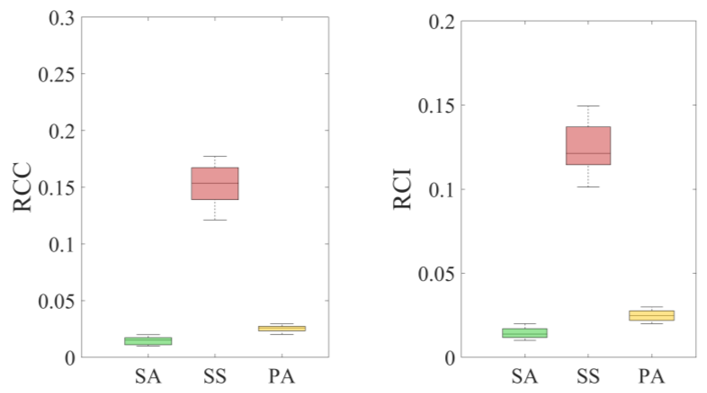
This study proposes the Redness Contribution Coefficient (RCC) and Reddening Rate Index (RCI) based on the RSSI index, which are adopted as phenological features for SS classification. RCC characterizes the inflection sharpness during the reddening stage and quantifies phenological curve asymmetry by comparing the average rising rate before the reddening peak with the declining rate after the peak. RCI measures the dynamic reflectance variation throughout the reddening process and evaluates the contribution of reddening signals to annual spectral characteristics via the ratio of RSSI integral over the reddening window (SORP–EORP) to that over the full growing season (SOS–EOS). Closely linked to betalain metabolism in SS, the two indices integrate temporal and spectral reddening signatures to enable accurate species discrimination. Figure 7 illustrates the expected discriminative capacity of RCC and RCI, where SS is anticipated to exhibit higher median values than SA and PA. The relevant formulas are calculated as follows:

$$RCC={\displaystyle \frac{(RSSIMV-RSSISOS)/(PRP-SOS)}{(RSSIMV-RSSIEOS)/(EOS-PRP)}}$$

(7)

$$RCI={\displaystyle \frac{{\int }_{SORP}^{EORP}RSSI\left(t\right) dt}{{\int }_{SOS}^{EOS}RSSI\left(t\right) dt}}$$

(8)

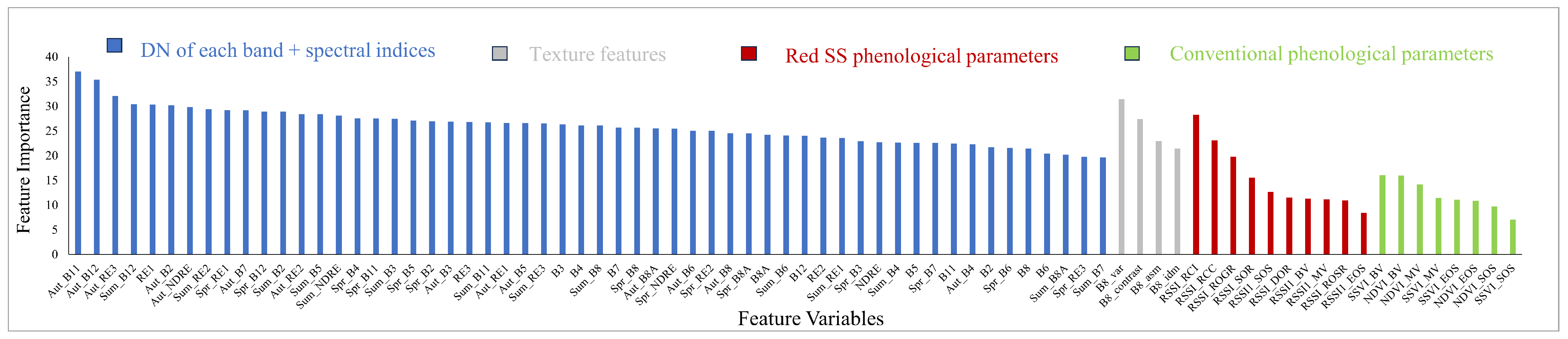
Simultaneously, this study constructed multi-dimensional classification features based on the Google Earth Engine platform. First, the original band features were used as the basic input to the classification model. Multispectral bands including B2, B3, B4, B5, B6, B7, B8, B11, and B12 were selected to preliminarily characterize the basic spectral properties of surface features. Simultaneously, this study comprehensively constructed a series of spectral indices: NDVI, Enhanced Vegetation Index (EVI), and Green Cover Index (GCI). By quantifying the reflectance differences of different band combinations, the study captured differences in vegetation growth status, water content, and spectral characteristics. In non-vegetation identification, a two-step strategy was adopted to account for the availability of surface water data. For 2019, the Joint Research Centre (JRC) Global Surface Water dataset [31] was used as the static water mask. For 2022–2025, because the JRC dataset is only updated up to 2021, this study used the Normalized Difference Water Index (NDWI) to dynamically identify water bodies. NDWI demonstrates excellent accuracy and stability in water extraction from Sentinel-2 imagery, ensuring the reliability of time-series analysis. The NDWI, along with the Normalized Difference Built-up Index (NDBI) and Bare Soil Index (BSI), was combined through a dynamic threshold method to construct a non-vegetation mask, effectively eliminating interference from buildings, bare soil, and water bodies.

In addition, a tidal inundation frequency feature was calculated for each target year using Sentinel-2 images acquired between May and October of that year. The May–October window was selected because it represents the period of highest tidal activity in the study area, best capturing spatial differences in inundation patterns across the intertidal zone. For each image, NDWI was computed and thresholded at 0.2 to generate a water/non-water mask. This threshold was determined empirically by examining the NDWI value distribution over typical water bodies (e.g., tidal creeks, open water) and non-water surfaces (e.g., vegetated areas, bare flats) in the study area, where water pixels consistently showed NDWI > 0.2. The inundation frequency per pixel was then derived as the proportion of water observations across all images in the May–October window and was incorporated into the multi-dimensional feature set to account for elevation-dependent submersion patterns of different vegetation types.

At the same time, the Red Edge Index Point (REIP) and Red Edge Slope Indices (RE1, RE2, RE3) [32] were introduced to fully utilize the high sensitivity of Sentinel-2 red-edge bands to the vegetation chlorophyll content and growth status, further improving the discrimination accuracy of halophytic plant communities. Since summer is the peak growing season for coastal wetland vegetation, with high vegetation coverage and stable spectral signals, the near-infrared band (B8) is most sensitive to the canopy structure, biomass, and spatial heterogeneity, effectively capturing spatial distribution differences among various vegetation communities. Therefore, seven texture features [33] were extracted from the summer B8 band using a 3 × 3 moving window and are selected to supplement the spatial heterogeneity information of vegetation communities (

Table 3. Classification feature set.

Feature Subset	Variable Abbreviation
Band characteristics	B2, B3, B4, B5, B6, B7, B8, B11, B12
Vegetation Index	NDVI, EVI, GCI
Water Index	JRC, NDWI
Built-up Index	NDBI
Bare Soil Index	BSI
Red edge Index	REIP, RE1, RE2, RE3
Texture features (Summer B8 band)	Mean Value, Homogeneity, Contrast, Dissimilarity, Entropy, Angular Second Moment, Correlation

).

2.3.2. Classification Methods and Accuracy Assessment

Random Forest (RF) [34] is an ensemble supervised learning method that generates multiple training subsets through bootstrap sampling to construct classification trees and randomly selects features when splitting nodes to enhance model diversity. This mechanism can effectively handle high-dimensional remote sensing features and adapt to the complex land cover types of coastal wetlands. The final classification decision was made by combining the results of all decision trees through voting, improving classification robustness. The model used in this study consists of 150 decision trees, reduced feature correlation by introducing random subspaces, and setting the minimum number of samples per leaf to five to suppress overfitting. These parameters were determined based on empirical standards in remote sensing classification and the default optimal settings of the Google Earth Engine (GEE) platform, without grid search or cross-validation, as they have been widely validated in comparable wetland vegetation classification studies.

After the classification was completed, this study optimized the results using the SNIC-based GEE built-in object-oriented segmentation method, which features high computational efficiency, a low salt-and-pepper effect, and suitability for processing large-area remote sensing images [35]. The optimal segmentation parameter combination was determined through the iterative testing of segmentation scales (8, 12, 16, 20, 24), compactness (0.05, 0.1, 0.2), and connectivity (4, 8). The final parameters were set as follows: segmentation scale = 16, compactness = 0.1, and connectivity = 8. Scale 16 provided the best trade-off between segmentation quality and computational feasibility: smaller scales (8, 12) resulted in excessive over-segmentation and increased processing time, while larger scales (20, 24) caused under-segmentation (merging of distinct vegetation patches) and triggered memory overflow errors in the GEE environment. The compactness parameter of 0.1 was selected to preserve natural patch boundaries without excessive regularization, and connectivity of 8 was chosen to maintain spatial continuity of vegetation patches. These parameters enabled automated and high-precision extraction of salt marsh vegetation such as SS, SA, and PA in the study area.

A classification accuracy evaluation is a key step in verifying the reliability of extraction result. This study used confusion matrix and its derived indices for quantitative evaluation [36]. Among them, producer accuracy reflects the classifier’s ability to identify actual land objects from the perspective of class authenticity, while user accuracy measures the probability of the class being correctly classified from the perspective of result usability. Overall accuracy and Kappa coefficient comprehensively evaluate the classification effect from the perspectives of overall consistency and non-random consistency, respectively. To ensure the statistical robustness of the evaluation, the samples were usually divided into training set and test set according to a certain ratio (e.g., 7:3) to ensure that the generalization ability of the model is effectively verified.

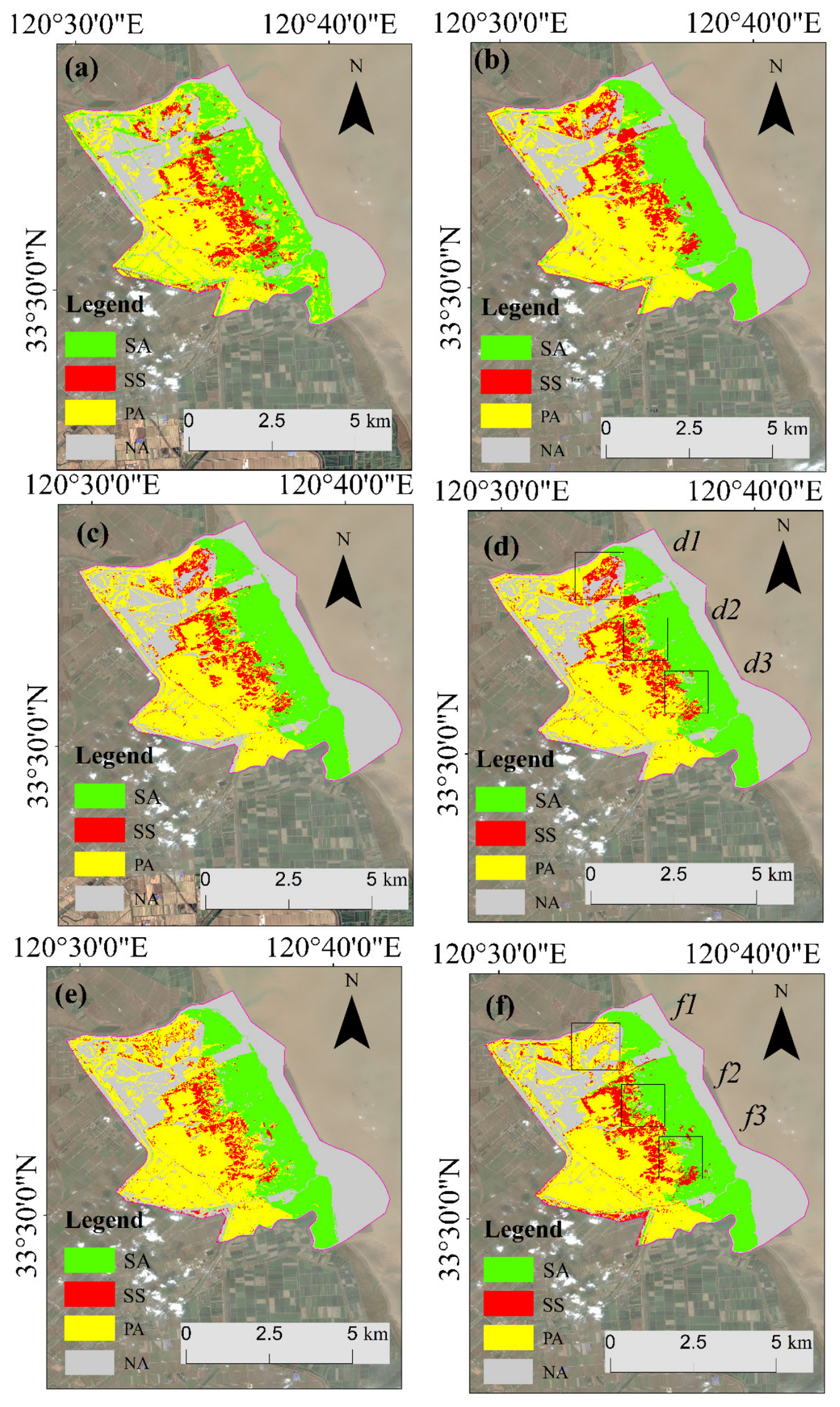
To systematically explore the impact of different image-synthesis methods and combinations of classification features on the classification accuracy of coastal wetland vegetation, this study designed six comparative schemes to conduct classification experiments (

Table 4. Classification scheme table.

Scheme	Image Information	Classification Features
Scheme 1	Median composite of images throughout the year	DN of each band + spectral indices + texture features
Scheme 2	Combined images acquired at spring, summer and autumn	DN of each band + spectral indices + texture features
Scheme 3	Combined images acquired at spring, summer and autumn	DN of each band + spectral indices + texture features + conventional phenological parameters
Scheme 4	Combined images acquired at spring, summer and autumn	DN of each band + spectral indices + texture features + conventional phenological parameters + red SS phenological parameters
Scheme 5	Autumn single-season images	DN of each band + spectral indices + texture features + conventional phenological parameters
Scheme 6	Autumn single-season images	DN of each band + spectral indices + texture features + conventional phenological parameters + red SS phenological parameters

). First, the median composite of images from all year round combined with the DN of each band, spectral indices, and texture features was used as the baseline scheme (Scheme 1). Based on this, to fully utilize the seasonal differences in vegetation, a three-season composite image scheme for spring, summer, and autumn was constructed (Scheme 2), and the classification performance differences between the single-temporal composite and multi-season composite were compared under the same features as Scheme 1. Second, to explore the impact of vegetation growth patterns on classification results, conventional phenological parameters were introduced on the basis of the three-season composite images (Scheme 3) to enhance the phenological separability of different vegetation types. Subsequently, considering the unique seasonal spectral characteristics of SS, the phenological parameters of SS constructed by our research team, as well as the RCC and RCI-specific phenological parameters proposed in this study, were incorporated (Scheme 4). Considering that the typical red spectral features of SS are mainly concentrated in autumn, to verify the feasibility of using autumn single-season images to simplify data volume, improve classification efficiency, and ensure classification accuracy, this study further designed two comparative schemes using only autumn composite images: Scheme 5 used autumn images as input, fusing the DN of each band, spectral indices and conventional phenological parameters; Scheme 6 supplements Scheme 5 with specific phenological parameters of red SS. Based on the above schemes, the classification potential of autumn single-season images combined with specific features was evaluated, and the classification accuracy of each scheme is shown in

Table 5. Comparative analysis of multiple feature combination methods.

Scheme	Image Information	Classification Features	Overall Accuracy	Kappa Coefficient
Scheme 1	Median composite of images throughout the year	DN of each band + spectral indices + texture features	0.7545	0.6335
Scheme 2	Combined images acquired at spring, summer and autumn	DN of each band + spectral indices + texture features	0.8390	0.7407
Scheme 3	Combined images acquired at spring, summer and autumn	DN of each band + spectral indices + texture features + conventional phenological parameters	0.8768	0.8202
Scheme 4	Combined images acquired at spring, summer and autumn	DN of each band + spectral indices + texture features + conventional phenological parameters + red SS phenological parameters	0.9732	0.9625
Scheme 5	Autumn single-season images	DN of each band + spectral indices + texture features + conventional phenological parameters	0.7891	0.7089
Scheme 6	Autumn single-season images	DN of each band + spectral indices + texture features + conventional phenological parameters + red SS phenological parameters	0.8943	0.8306

.

3. Results

3.1. Classification Result Accuracy Analysis

3.1.1. Seasonal Composite-Based Classification

This study used the 2019 Jiangsu Yancheng Wetlands and Rare Birds National Nature Reserve as an example. Based on Sentinel-2 imagery (cloud cover below 20%), it com-pared the classification performance of the year-round composite imagery with that of the spring, summer, and autumnal equinox composite images using only spectral index features. The overall accuracy and Kappa coefficient are shown in Table 5. The overall classification accuracy of the year-round composite imagery was 0.7545, and the Kappa co-efficient was 0.6335 (Scheme 1, Figure 8a). In contrast, the seasonal composite imagery improved the overall accuracy to 0.8390 and the Kappa coefficient to 0.7407 (Scheme 2, Figure 8b). From the spatial distribution of the classification results, the boundary between SA and PA was blurred in the annual synthesis, especially in the intertidal transition zone where there were many misclassifications. The seasonal composite reduced such misclassifications and generated more distinct spatial patterns: SS was distributed in patches in the mid-tidal flats, PA was concentrated in the near-shore high flats, and the seaward expansion of SA was more visually distinct [37,38,39].

Although the detailed scheme comparison was performed for the 2019 Yancheng Reserve sub-area as a representative benchmark, the seasonal composite strategy was applied consistently across all years (2019–2025) and the entire Jiangsu Province. Consistent spatial patterns were observed across Lianyungang, Yancheng, and Nantong.

3.1.2. Conventional Phenological Parameters Classification

Compared with single-phase images, seasonal composite images yielded higher classification accuracy for coastal wetland vegetation. However, within-season spectral fluctuations may reduce the observability of key phenological events. Based on three-season composite images, conventional phenological parameters derived from NDVI and SSVI were added (Scheme 3, Figure 8c). The overall accuracy reached 0.8768, and the Kappa coefficient reached 0.8202 (Table 5), representing increases of 3.78% and 0.0795 compared with Scheme 2. From the spatial characteristics of the classification results, the boundaries between SA and PA were clearer, and spectral mixing in the intertidal transition zone was further reduced.

3.1.3. Classification Based on Phenological Parameters of SS

Scheme 4 (Figure 8d) was formed by adding the red SS phenological parameters (RCC and RCI) proposed in this study to Scheme 3. The overall accuracy reached 0.9732, and the Kappa coefficient reached 0.9625 (Table 5), representing increases of 9.64% and 0.1423 compared with Scheme 3. Spatially, SS patches showed clearer boundaries and higher spatial consistency. Classification accuracy in NA (water bodies and tidal flats) was also increased. As shown in the confusion matrix

Table 6. Accuracy evaluation results of confusion matrix for Scheme 4.

Classification	SA	SS	PA	NA	User Accuracy (%)
SA	211	1	0	1	97.68
SS	1	135	0	1	98.54
PA	3	0	88	2	94.62
NA	1	1	3	75	93.75
Producer accuracy (%)	98.06	98.54	96.70	94.94

, Scheme 4 achieved a user accuracy of 98.54% for SS, 98.06% for SA, and 96.70% for PA. Table 6 presents validation results for the Yancheng Reserve sub-area as a benchmark. The method was subsequently applied to the entire Jiangsu Province (Section 3.2).

Two additional schemes were tested using autumn single-season images. Scheme 5 (Figure 8e) employed autumn composite images with the same features as Scheme 3, yielding an overall accuracy of 0.7891 and a Kappa coefficient of 0.7089. Scheme 6 (Figure 8f) was formed by adding red SS phenological parameters to Scheme 5, increasing the overall accuracy to 0.8943 and the Kappa coefficient to 0.8306 (Table 5). Spatial classification of SS was improved in Scheme 6, but overall accuracy remained lower than that of Scheme 4. Obvious misclassification between SA and PA was observed in the upper intertidal zone, with blurred boundaries and overlapping patches.

As shown in Figure 9, the zoomed-in views (d1–d3, f1–f3) display differences between Scheme 4 and Scheme 6. SS patches in Scheme 6 were more fragmented, while those in Scheme 4 were more contiguous. Discrimination between PA and SA was improved in Scheme 4, with clearer boundaries and fewer misclassifications. Scheme 4 was selected as the optimal classification scheme.

The confusion matrix shows validation results for the Jiangsu Yancheng Wetlands and Rare Birds National Nature Reserve (523 validation points). The methodological framework (Scheme 4) was then applied to the entire Jiangsu Province; spatial patterns are discussed in Section 3.2. Overall Accuracy = 97.32%; Kappa = 0.9625. SA: Spartina alterniflora; SS: Suaeda salsa; PA: Phragmites australis; NA: non-vegetated area.

3.1.4. Model Validation

To comprehensively assess the robustness and generalizability of the optimal classification scheme (Scheme 4), three complementary validation strategies were implemented.

Feature importance analysis [40]. Feature importance values were extracted from the Random Forest model. As shown in Figure 10, spectral bands from spring (Spr) and autumn (Aut) composites exhibited the highest importance scores. RCI and RCC ranked first and second among all phenological features (9th and 24th among 86 features in total). Texture features exhibited moderate contributions, mainly from the summer B8 band.

Spatial cross-validation [41]. A 5-fold spatial cross-validation was conducted using geographic blocks. As shown in

Table A1. Accuracy results of 5-fold spatial cross-validation for Scheme 4.

Land Cover Type	User Accuracy	Producer Accuracy
Spartina alterniflora (SA)	0.9646	0.9870
Suaeda salsa (SS)	0.9670	0.9647
Phragmites australis (PA)	0.9547	0.9425
Non-vegetated area (NA)	0.9754	0.9392
Overall Accuracy (OA)	0.9652	-
Kappa coefficient	0.9513	-

, the mean overall accuracy was 96.52% and the Kappa coefficient was 0.9513, consistent with the original hold-out validation (97.32%).

Independent external validation. An independent validation dataset not used in training was applied. This validation yielded an overall accuracy of 95.04% and a Kappa value of 0.9303 (

Table A2. Accuracy results of independent external validation for Scheme 4.

Land Cover Type	User Accuracy	Producer Accuracy
Spartina alterniflora (SA)	0.9352	0.9951
Suaeda salsa (SS)	0.9820	0.9316
Phragmites australis (PA)	0.9588	0.9394
Non-vegetated area (NA)	0.9375	0.8824
Overall Accuracy (OA)	0.9504	-
Kappa coefficient	0.9303	-

).

Statistical significance testing and ablation analysis. McNemar’s test [42] with continuity correction was conducted based on 523 validation points. Between Scheme 4 and Scheme 3, Scheme 4 correctly classified 118 more samples (c = 120 vs. b = 2), with a chi-square statistic of 112.20 (p < 0.001). Between Scheme 4 and Scheme 6, Scheme 4 correctly classified 16 more samples (c = 28 vs. b = 12), with a chi-square statistic of 5.625 (p < 0.05).

3.2. GIS-Based Vegetation Change Analysis

3.2.1. Quantity Change Analysis

Using seasonal composite imagery and a classification method incorporating multi-dimensional phenological features, the area of coastal wetland vegetation in Jiangsu Province in 2019, 2022, 2024, and 2025 was obtained.

Table 7. Coastal wetland vegetation transfer matrix in Jiangsu Province, 2019–2025 (Unit: km²).

Classification	SA	SS	PA	NA	Total in 2025
SA	5.11	6.29	5.50	167.46	184.37
SS	0.98	23.98	19.36	69.44	113.75
PA	1.27	51.27	111.43	198.06	362.02
NA	9.15	90.18	135.58	3781.24	4016.15
Total in 2019	16.50	171.72	271.88	4216.19	4676.29

shows the vegetation transfer matrix of coastal wetlands in Jiangsu Province from 2019 to 2025. The area of SA decreased from 184.37 km² in 2019 to 16.50 km² in 2025, with a reduction rate of over 90%. SA in treated areas was mainly converted to NA, SS, and PA. Of these, 90.8% of SA was converted to NA, 3.41% to SS, and 2.98% to PA.

From the transfer matrix, 61.0% of SS and 54.7% of PA were converted to NA. As shown in the time series dynamics (Figure 11), the area of SA decreased continuously from 185.88 km² in 2019 to 16.50 km² in 2025. The area of SS increased from 2019 to 2024 and decreased in 2025. The area of PA showed a fluctuating downward trend from 2019 to 2025.

The transfer matrix may be influenced by inter-annual variability in phenology and environmental conditions; see Section 4 for limitations.

3.2.2. Analysis of Changes in Vegetation Distribution in Different Regions

This subsection describes the spatiotemporal patterns of vegetation dynamics.

(1)

Results of dynamic monitoring of vegetation in coastal wetlands of Lianyungang City

From 2019 to 2025, the area of SA in Lianyungang showed a decreasing trend. From 2019 to 2022, the area of SA increased by approximately 35%. The area of SS decreased by 12.8%, and the area of PA decreased by 8.3%. From 2022 to 2024, the area of SA decreased by 78%, with a total reduction of 16.28 km². Of the converted area, 17.7% was transformed into SS and 5.2% into PA. The area of SS increased by 42% compared with 2022. From 2024 to 2025, the area of SA further decreased. The area of SS was 11.01 km² in 2025, of which 44.7% remained stable and 12.2% was converted to PA. The area of PA remained stable at approximately 25 km², and 39.1% of PA was converted to SS (Figure 12).

Spatially (Figure 13), from 2019 to 2022, contiguous patches of SA were observed in the three estuarine wetlands. From 2022 to 2024, the distribution of SA became fragmented, and the area of NA increased by approximately 15%. From 2024 to 2025, the area of SS and PA in the eastern part of Linhong Estuary Wetland increased by 28% compared with 2024. The area of PA and SS in Liezi Estuary Wetland increased. The total vegetation area in Ganyu Estuary Wetland decreased slightly.

(2)

Results of dynamic monitoring of vegetation in coastal wetlands of Yancheng City

From 2019 to 2025, vegetation changes in Yancheng coastal wetlands were recorded. From 2019 to 2022, the area of SA increased from approximately 132.38 km² to a peak. The area of SS decreased by 38%, and the area of PA increased by 12.7%. From 2022 to 2024, the area of SA decreased by 82%. The area of PA increased by 52.1%, and the area of SS showed a slight recovery. From 2024 to 2025, the area of SA decreased by more than 90%. The area of PA increased by 9.3%, and the area of SS decreased (Figure 12).

In terms of spatial distribution (Figure 14), from 2019 to 2022, continuous distribution of SA was observed at the Yancheng Wetlands and Rare Birds National Nature Reserve and Tiaozini Wetland. From 2022 to 2024, the area of SA decreased, and scattered patches of native vegetation appeared. From 2024 to 2025, SS and PA became the dominant vegetation types. Vegetation coverage increased by 18% compared with 2024.

(3)

Results of dynamic monitoring of vegetation in coastal wetlands of Nantong City

From 2019 to 2025, vegetation variations of Nantong coastal wetlands were presented below. From 2019 to 2022, the total vegetation area rose by 23%. SA expanded by 41%, and the area of SS peaked at approximately 68.3 km². From 2022 to 2024, the area of SA declined by 75%, with a total reduction of 31.08 km²; 7.5% of the converted area shifted to SS and 6.1% shifted to PA. The PA area dropped by 8.5%, and the SS area fluctuated downward. From 2024 to 2025, over 90% of SA was reduced. The PA area grew by 16.7% to around 76 km²; 20.7% of PA remained unchanged, and 17.3% transferred into SS, with the total SS area reaching approximately 60.72 km² (Figure 12).

In terms of spatial patterns (Figure 15), obvious vegetation changes were observed at Xiaoyangkou coastal wetland of Rudong County. From 2019 to 2022, contiguous SA patches mixed with native vegetation were distributed across tidal flats. From 2022 to 2024, SA coverage shrank rapidly and bare ground expanded temporarily. From 2024 to 2025, SS and PA became the dominant vegetation types, and vegetation coverage remained above 65%.

4. Discussion

This study improves coastal wetland vegetation classification by integrating multi-seasonal spectral bands, spectral indices, and SS-specific autumn-reddening phenological parameters. The optimal Scheme 4 reaches an overall accuracy of 97.32% with a Kappa coefficient of 0.9625, which supports large-area long-term dynamic monitoring of regional Spartina alterniflora (SA) removal outcomes across Jiangsu coastal wetlands. High classification accuracy provides reliable basic data for local wetland conservation and invasive species management.

4.1. Biological Mechanism and Spectral Discriminant Principle of RCC and RCI

The two newly constructed indices, RCC and RCI, are developed based on the unique autumnal reddening physiology of Suaeda salsa (SS). During the leaf-reddening period, betalain accumulation and cell structure degradation jointly raise the shortwave infrared reflectance and reduce near-infrared reflectance of the SS canopy, forming unique seasonal spectral characteristics that differ distinctly from perennial green Phragmites australis (PA) and evergreen exotic SA. RCC quantifies the asymmetric feature of annual phenological curves centered on the reddening peak, while RCI accumulates the total spectral deviation induced by pigment variation across the whole growing season. The combined application of RCC and RCI effectively enlarges interspecific spectral differentiation and reduces mixed-pixel misclassification in intertidal transition zones.

Compared with existing single-time-window SS indices such as SSVI and SSSI, RCC and RCI take full-season phenological fluctuation into consideration and maintain stable identification capacity under variable tidal inundation and latitudinal environmental gradients, which is validated by spatial cross-validation (OA = 96.52%) and independent sample validation (OA = 95.04%). McNemar’s test further statistically confirms that supplementing RCC and RCI significantly promotes classification performance relative to the conventional phenology-only Scheme 3 (p < 0.001).

4.2. Method Transferability and Comparison with Previous Published Studies

The established classification workflow based on seasonal composite imagery plus red-phenology indices has favorable transfer potential for temperate coastal wetlands dominated by autumn-reddening halophytes. Core technical links including the multi-temporal median composition, Fourier-based phenology fitting, and Random Forest classification can be transplanted to other temperate or subtropical estuarine regions after localized calibration of phenological parameters.

Most previous wetland classification studies in Jiangsu only adopted single-date or annual median composite Sentinel-2 datasets; the introduction of triple-season composite and SS autumn-reddening features improves overall mapping accuracy by 9–15%. Consistent inter-city spatial changing rules of SA, SS, and PA across Lianyungang, Yancheng, and Nantong further verify the regional robustness of the proposed feature combination strategy.

4.3. Performance Comparison with Deep Learning Segmentation Approaches

In contrast to mainstream deep learning segmentation models (U-Net, SegFormer), our Random-Forest-driven feature engineering method requires fewer manually labeled field samples and achieves lower computing consumption for large-scale coastal mapping tasks. Deep learning can capture complicated contextual spatial information from abundant training data, yet its performance is highly susceptible to sample scarcity, class imbalance, and label noise, limiting routine operational application in sparsely surveyed wetland zones. The stable high accuracy above 95% in two types of validation demonstrates that our approach is a feasible alternative for long-term operational wetland monitoring when massive annotated datasets are unavailable.

4.4. Ecological Implications Derived from Multi-Year Vegetation Dynamic Changes

From 2019 to 2025, the SA area in Jiangsu was reduced by over 90%, reflecting remarkable achievements of provincial large-scale invasive plant governance. However, approximately 90.8% of the original SA mudflat was converted to bare non-vegetated land rather than native SS and PA communities. Meanwhile, 61.0% of original SS and 54.7% of original PA were transformed into unvegetated flats, indicating the insufficient natural spontaneous restoration of native species after alien plant removal.

According to the quantitative conversion characteristics revealed by multi-year mapping results, three targeted restoration suggestions for coastal wetland management are proposed: (1) implement artificial SS reseeding on mid-tidal flats with slow natural colonization; (2) prioritize PA supplementary plantation on nearshore high flats with relatively low soil salinity; (3) sustain at least two consecutive years of post-clearance monitoring to prevent SA secondary invasion and combine mechanical eradication with native vegetation reconstruction.

4.5. Uncertainty Sources, Parameter Sensitivity, and Scalability Limitations

Multiple inherent uncertainties restrict the universal scalability of the proposed classification framework. First, Sentinel-2’s 10 m spatial resolution cannot capture tiny scattered vegetation patches and narrow ecotone boundaries; its 5-day revisit cycle is frequently blocked by cloud cover, missing abrupt phenological shifts triggered by extreme drought or heat anomalies. Interannual climatic fluctuations alter key phenological timings including SOS, SORP, and EORP, leading to unavoidable errors during phenological extraction even after SG smoothing and threshold optimization.

Fixed empirical thresholds (70% for SORP, 50% for EORP) are used to identify critical phenological nodes in this research, whereas systematic parameter sensitivity analysis regarding threshold fluctuation effects on final classification accuracy is not completed, forming a prominent uncertainty source. Spectral mixing of vegetation and exposed mud in transitional intertidal zones is mitigated via multi-feature fusion but cannot be entirely eliminated. Year-by-year independent model training is adopted to weaken interannual environmental interference, yet complete cross-year generalization is not guaranteed. Tidal fluctuation is roughly corrected via median compositing and the inundation frequency layer instead of pixel-scale tide-height filtering, lowering the mapping precision on low intertidal flats. In addition, the fixed SNIC segmentation scale constrains the extraction of ultra-small vegetation fragments.

Despite satisfying validation accuracy within Jiangsu Province, direct blind migration to coastal wetlands with a drastically different climate, tidal regime and soil background is not recommended.

4.6. Future Research Perspectives

Future studies will integrate high-resolution UAV/Planet time-series images and all-weather Sentinel-1 SAR data to compensate for the resolution deficiency and cloud interference; complete quantitative uncertainty quantification and systematic sensitivity test for phenological thresholds; develop adaptive multi-scale SNIC segmentation; and carry out cross-provincial experiments to further verify nationwide transferability of the index system. In addition, advanced deep learning algorithms will be combined with our RCC/RCI red-phenology indicators to improve fine-scale classification for heterogeneous wetland landscapes.

5. Conclusions

This study developed a phenology-based classification framework for coastal wetland vegetation using Sentinel-2 time-series data (2019–2025) and a random forest classifier. The integration of multi-seasonal composites and newly proposed phenological parameters (RCC, RCI) achieved the highest accuracy (97.32%, Kappa = 0.9625), overcoming the limitations of NDVI-based phenology and single-season imagery by capturing species-specific reddening and seasonal growth rhythms.

From 2019 to 2025, the SA area in Jiangsu decreased by more than 90%, with most cleared land converting to non-vegetated areas, demonstrating the effectiveness of national control actions. Concurrently, native vegetation showed overall degradation, highlighting the need for active restoration alongside invasive species removal. The proposed method enables a spatially explicit, quantitative assessment of control effectiveness and native vegetation dynamics, critical for adaptive management.

The framework is transferable to other coastal regions facing similar invasion challenges. It directly supports UN SDG 14 (Life Below Water) by contributing to sustainable coastal ecosystem management, and SDG 15 (Life on Land) by preventing the spread of invasive alien species and promoting native ecosystem restoration. By linking satellite-based classification with invasive species control and native vegetation restoration, this study provides a practical, scalable tool for large-scale, evidence-based coastal wetland management that can be adapted to other regions with similar phenological dynamics.