A Proposal for Selecting a Pareto Solution with Desirable Properties

Abstract

Decision making at both the strategic and operational levels in industrial and non-industrial organizations requires a compromise among economic, social, and environmental criteria. However, doing so on an empirical or expert sensitivity base is not recommendable. A robust approach is proposed to help the decision-maker in selecting a solution from the Pareto set, which is not a current practice. The approach involves applying various multi-criteria decision-making methods to select a Pareto-optimal solution with four key properties: low bias, high prediction quality, high resilience, and high robustness. These properties can be prioritized based on the decision-maker’s preferences. However, in order to take the decision maker’s uncertainty into account, various sets of weights are generated. Solution discrimination and validation are performed using the Sum of Ranking Differences technique, which makes it possible to prune Pareto solutions and identify the best one from a statistical point of view. A case study demonstrates the proposed approach’s usefulness, and it is apparent that changing the weight of Pareto-optimal solution properties, the most favorable solution, validated by the Sum of Ranking Differences technique, should change accordingly.

1. Introduction

It is widely accepted that present human needs should not compromise the ability of future generations to achieve their own needs from an environmental, economic, and social point of view. The genesis and theoretical foundations of these sustainability dimensions have been discussed in the literature [1], and many organizations are already integrating the economic, environmental, and social dimensions of sustainability [2,3]. Despite ongoing debate about how these dimensions should be prioritized and/or integrated, their relevance is widely acknowledged across all business sectors [4]. From classic engineering areas like chemical, electrical, mechanics, and materials to more recent knowledge areas like biomedical and bioinformatics, the quantity and variety of studies addressing sustainability issues is significant [5].

Most sustainability issues require a compromise among economic, social, and/or environmental criteria associated with processes and products, so multi-criteria decision-making methodologies, methods, and tools are often used by decision-makers to support more informed and balanced decisions. The design and development of products, technology, marketing, and operations management strategies, financial investments, and governance politics are examples of problems faced by managers, engineers, politicians, etc., that cannot or must be solved empirically (see illustrative case studies in Refs. [2,5,6,7,8,9,10]).

Problems with multiple conflicting objectives (functions that are mathematical descriptions of process and/or product variables, usually conflicting with each other) exist in all science fields, and many theoretical and applied case studies have been published in the literature [11,12]. For these problems, no single solution exists, and none of the available solutions to solve those problems yield the desired value for each objective. A representative and complete set of solutions should be generated for such problems. This way, the decision-maker can take a comprehensive view of all possible trade-offs and identify the solution of his/her preference, considering technical and/or economic requirements. However, when the number of optimal solutions is excessively large, it becomes difficult, if not impossible, for the decision-maker to select the most favorable one. This comes about when, in addition to the number of solutions, the solution’s properties must be considered in the solution selection process.

In [13], the authors argue that, in addition to Bias (objectives’ deviation from their target value), the solutions prediction quality (objectives’ variance due to their models coefficients uncertainty), Resilience (objectives’ sensitivity to perturbations in the input variable settings of objective functions, truncation and rounding), and robustness (objectives’ insensitivity to noise factors) are objective’s properties that impact on the quality of solutions to multi-objective problems. According to those authors, the reproducibility of nondominated solutions will be higher if these objectives’ properties are considered in the selection of a solution from the Pareto set. In addition, it avoids wasting resources and time in generating, selecting, and implementing a theoretical optimal solution that does not produce the expected outcomes. This is further exacerbated in expensive optimization domains like those requiring time-consuming computer simulations as example. However, if their recommendation is adopted, the solution selection becomes a multi-attribute problem, and many methods can be used for solving it, i.e., to select an optimal solution from the Pareto set.

A desirability-based method to identify the most favorable optimal or nondominated solution for multi-objective problems was proposed in [14]. The authors demonstrated the usefulness and relevance of their proposal, contributing to fill a gap in the literature. In fact, the number of papers dealing with the selection of a solution from the Pareto set is still very low, just as other authors had previously noted [15,16,17]. In some multi-objective problems published in the literature, namely in top journals, the Pareto set is not even generated. Among the small number of published papers where the Pareto set is generated, the so-called Technique for Order Preference by Similarity to Ideal Solution (TOPSIS) is a very popular method for identifying the most favorable optimal solution [14,18].

The variety and quantity of Multiple Attribute Decision Making (MADM) methods that are alternatives to TOPSIS is huge. A review on the evolution of those methods over the last five decades is presented in [19], and it is widely accepted that no method performs better than any other in every problem. Using more than one MADM method has been a current practice. However, when most methods suggest a different optimal solution, a critical question remains: Which solution must the decision-maker select to solve its problem? To help the decision-maker in selecting a solution from the Pareto set, a new approach is exposed and illustrated in the next sections. The approach involves applying various multi-criteria decision-making methods to select a Pareto-optimal solution with four key properties: low bias, high prediction quality, high resilience, and high robustness. Pareto solution selection accounts for uncertainty in the decision-maker’s assessment of properties by employing various sets of weights. The solution discrimination and validation are performed using the Sum of Ranking Differences (SRD) technique. This is a widely used technique which enables the pruning of the Pareto solutions and the identification of the most favorable one. SRD is conceptually related to the popular Spearman’s Rank correlation and Kendall’s Tau measures, as all of them rely on ordinal information to assess relationships among variables. However, several substantive distinctions should be noted. SRD employs a fixed reference ranking against which all alternatives are evaluated, whereas Kendall’s Tau and Spearman’s Rank correlation coefficients are generally used in pairwise or multivariate settings without the need for an explicit reference ranking. Furthermore, SRD constitutes a true distance metric, computed as the L1 norm (Manhattan distance or taxicab distance) of the differences between ranks, in contrast to the number of inversions between two rankings (Kendall’s Tau measure) and the rank-based correlation coefficient (Spearman’s Rank correlation), which is derived from the product-moment formulation applied to ranked data. Regarding SRD utility and efficacy, the reader is referred to Refs. [20,21,22,23,24,25]. Thus, the proposed approach aims to provide the decision-maker with a robust framework for selecting a solution with high reproducibility from the Pareto set.

The remainder of the paper is structured as follows: the proposed approach for selecting a solution from the Pareto set is introduced in the next section; Section 3 includes a case study and discusses the results; the Conclusion is presented in Section 4.

2. A New Approach for Selecting an Optimal Solution from the Pareto Set

Multiple objective decision making, also called multi-objective optimization (MOO), aims to identify a set of optimal or nondominated solutions that satisfy the decision-maker’s constraints and preferences by optimizing multiple objective functions (mathematical descriptions of process and/or product variables, usually called responses) that are usually conflicting with each other. The major developments over the last five decades, namely theoretical advancements, approaches, and applications in different functional areas, current research trends, and future directions are discussed in [26]. These authors state that the interest and publications in the area are significant and are growing very fast. Advances in computing technology have significantly contributed to this evolution, enabling the analysis of increasingly large and complex problems through sophisticated (exact and heuristic) search algorithms. For a review in the development of heuristic methods over the last 50 years, the reader is referred to [27], and a list of open-source programs and some commercial software for running them is presented in [17].

In an increasingly complex and fast-changing world, decision-makers often need to find the most favorable solution to multi-objective optimization problems they need to solve. Thus, under the assumption that they have access to the literature and can identify the most appropriate approach for generating a representative Pareto set [28], an ultimate difficulty consists in selecting a solution from the Pareto set. All the named Pareto solutions are optimal and, theoretically, they are equally useful. However, the compromise among the objective functions is not the same for each optimal (non-dominated) solution [29].

MADM methods have proven to be an effective substitute for empirical-based or expert sensitivity-based tasks for identifying a solution from the Pareto set that produces the best compromise among multiple attributes. The methods differ in many dimensions, namely, in complexity (the way in which preferences and evaluation criteria are represented), type of data aggregation (the possibility of including uncertain data), and the availability of implementations in decision support systems or the degree to which criteria can be compensated [30]. Extensive reviews on those methods are presented in [19,31,32]. Examples of reviews on applications in specific fields, for instance, in financial management, and environmental and water resources planning and management, are presented in [33,34]. However, despite the availability of multiple MADM methods, there is no one that performs better than all the others in every situation. To use more than one method is a current practice, but their discrimination and validation are a practical need that is addressed in the next sections of this paper, in addition to attribute-weighting uncertainty, with the purpose of selecting a solution from a Pareto set.

2.1. Multi-Attribute Decision-Making Methods

The main purpose of MADM methods can be to choose, rank, sort, or cluster the actions (alternatives, solutions, options, acts, candidates, etc.) considering conflicting attributes (characteristics, properties, … of a process, a product and/or a service). Ranking is the process of ordering alternatives by preference, sorting is to assign alternatives to predefined preference-ordered categories, choosing is to select a single alternative, or a subset of alternatives, that meets specific preference requirements, and clustering is to group alternatives based on similarity features or on preference relations. Despite the availability of multiple MADM methods, the need to handle a wider variety of more complex decision scenarios has made the development of hybrid MADM methods an active research topic [35]. However, the high number of MADM methods, while commendable, may result in the so-called “confusion of abundance”. In addition, no method has proven to perform better than any other in every decision-making situation. In some cases, different methods led to the same best alternative, in other cases, they led to different alternatives. Thus, the choice of a MADM method is not a basic task, though guidelines exist for that purpose [32,36]. Examples of proper and improper uses of MADM methods were pointed out and discussed in [37]. Regarding the methods’ performance, various papers review them and evaluate their performance. Examples are [15,38,39,40,41,42,43,44,45], to cite only a few.

Ten structurally distinct methods were selected for the proposed approach to ensure diversity of results and minimize overlap. The chosen methods comprise popular and easy-to-implement techniques, making them particularly suitable for less experienced decision-makers addressing multi-attribute decision-making problems. The selected methods are the following: Desirability Geometric Mean; Weighted Sum; Weighted Aggregated Sum Product Assessment (WASPAS); Max–Min; Multi-objective optimization on the basis of the ratio analyses (MOORA); Utility; Technique for Order Preference by Similarity to Ideal Solution (TOPSIS); TOPSIS_N; Desirability Arithmetic Mean.

2.1.1. Desirability Geometric Mean

This method (Desirability_GM, [46]) has been used for solving multi-objective problems in various science fields [47,48]. The global desirability function ($D_i$) is a geometric mean of the individual desirability functions that take values between zero and one, where one is the most favorable value.

$$D_i={\left(\left(d_{i1}{)}^{w_1}\right(d_{i2}{)}^{w_2}\dots (d_{in}{)}^{w_n}\right)}^{{\displaystyle \frac{1}{\sum w_n}}}$$

(1)

where $w_j$ $(j= 1, \dots , n)$ are user-specified parameters (weights, with ${\displaystyle {\sum }_{j=1}^n}{w}_j=1$) and $d_{in}$ represents individual desirability functions ($d_{ij})$. The objective is to maximize $D_i \left(i= 1, \dots , m\right).$ When $D_i=1$, all the individual desirability yields the best value $\left(d_{ij}=1, \mathrm{for} \mathrm{any} i, j\right)$. When $D_i=0$, at least the value of one individual desirability is equal to its worst value $\left(d_{ij}=0, \mathrm{for} \mathrm{any} i, j\right)$. The individual desirability functions normalize the performance measures (attributes) and, smaller-the-better-type (STB-type) attributes, whose values are desired to be smaller than an upper bound, are defined as

$$d_{ij}=\left\{\begin{array}{c}0 , { x}_{ij}<\min \left(x_j\right)\\ {\left({\displaystyle \frac{x_{ij}-\max \left(x_j\right)}{{\mathrm{m}\mathrm{i}\mathrm{n}(x}_j)-\mathrm{m}\mathrm{a}\mathrm{x}(x_j)}}\right)}^s, {\mathrm{m}\mathrm{i}\mathrm{n}(x}_j)\le x_{ij}<\mathrm{m}\mathrm{a}\mathrm{x}(x_j)\\ 0 , x_{ij}>\max (x_j)\\ \end{array}\right.$$

(2)

where $x_{ij}$ is the performance measure (value) of the i-th alternative or solution ($A_i$ with $i=1, \dots , m)$ on the j-th criterion or attribute $(C_j \mathrm{w}\mathrm{i}\mathrm{t}\mathrm{h} j=1, \dots ,n)$, and s is a user-specified parameter whose value must be higher than zero. The tabular representation of $x_{ij}$ forms a matrix of size m × n called decision matrix.

For larger-the-better-type (LTB-type) attributes, whose value must be larger than a lower bound, the individual desirability function is defined as

$$d_{ij}=\left\{\begin{array}{c}0 , x_{ij}<{\mathrm{m}\mathrm{i}\mathrm{n}(x}_j)\\ {\left({\displaystyle \frac{x_{ij}-\mathrm{m}\mathrm{i}\mathrm{n}(x_j)}{\mathrm{m}\mathrm{a}\mathrm{x}(x_j)-\mathrm{m}\mathrm{i}\mathrm{n}(x_j)}}\right)}^s, {\mathrm{m}\mathrm{i}\mathrm{n}(x}_j)\le x_{ij}<{\mathrm{m}\mathrm{a}\mathrm{x}(x}_j)\\ 0 , x_{ij}\ge {\mathrm{m}\mathrm{a}\mathrm{x}(x}_j)\\ \end{array}\right.$$

(3)

The s values enable the shape of $d_{ij}$ to be changed. The higher the s values are, the greater the importance of the attribute values being closer to the respective target will be, i.e., the $d_{ij}$ value is very small unless the attribute value comes very close to its desired value for a large s value. For a small value of s, the $d_{ij}$ value will be large even when the attribute is distant from its desired value.

2.1.2. Weighted Sum Method (WSM)

The WSM is often used by researchers and practitioners, and the ${WSM}_i$ index value must be as high as possible.

$${WSM}_i={\displaystyle \sum _{j=1}^n}{w}_j{n}_{ij}$$

(4)

where $w_j$ are weights, with ${\displaystyle {\sum }_{j=1}^n}{w}_j=1$, and

$$n_{ij}={\displaystyle \frac{x_{ij}-\mathrm{m}\mathrm{i}\mathrm{n}\left(x_j\right)}{\mathrm{m}\mathrm{a}\mathrm{x}\left(x_j\right)-\mathrm{m}\mathrm{i}\mathrm{n}\left(x_j\right)}}$$

(5)

for LTB-type attributes, and

$$n_{ij}={\displaystyle \frac{\mathrm{m}\mathrm{a}\mathrm{x}\left(x_j\right)-x_{ij}}{\mathrm{m}\mathrm{a}\mathrm{x}\left(x_j\right)-\mathrm{m}\mathrm{i}\mathrm{n}\left(x_j\right)}}$$

(6)

for STB-type attributes.

2.1.3. Weighted Aggregated Sum Product Assessment (WASPAS)

The WASPAS method combines the WSM and Weighted Product Method (WPM). It sorts the alternatives based on the $Q_i^{12}$ index value, which must be as high as possible:

$$Q_i^{12}={\alpha Q}_i^1+(1-\alpha )Q_i^2$$

(7)

where $0\le \alpha \le 1$. The α value will be set to 0.5 in the case study presented here, what is a current practice. When $\alpha =0$, the WASPAS becomes a weighted product method. When $\alpha =1$, it becomes a weighted sum product. The relative importance of the i-th alternative $Q_i^1$ and $Q_i^2$ is calculated by (8) and (9), respectively.

$$Q_i^1={\sum }_{j=1}^n{w}_j{n}_{ij}$$

(8)

$$Q_i^2={\prod }_{j=1}^n{n}_{ij}^{w_j}$$

(9)

The $n_{ij}$ values for LTB-type attributes and for STB-type attributes are calculated by (10) and (11), respectively.

$$n_{ij}={\displaystyle \frac{x_{ij}}{\max \left(x_j\right)}}$$

(10)

$$n_{ij}={\displaystyle \frac{\min \left(x_j\right)}{x_{ij}}}$$

(11)

2.1.4. Max–Min

The Max–Min method aims at maximizing the minimum attribute value (12). This method is robust to potential dependences between attributes and accounts for their relative priority [49], which can be normalized by individual desirabilities (2) and (3).

$${Mm}_i=\mathrm{m}\mathrm{i}\mathrm{n}\left(d_{i1}/w_1, d_{i2}/w_2, \dots ,d_{ij}/w_n\right)$$

(12)

2.1.5. Utility

The Utility method has been also often used to support the decision making in multi-attribute problems, and consists in transforming the $x_{ij}$ into a preference score $\left(P_{ij}\right)$ as follows:

$$P_{ij}=S_j \log \left({\displaystyle \frac{x_{ij}}{\mathrm{m}\mathrm{i}\mathrm{n}\left(x_j\right)}}\right)$$

(13)

where $S_j$ is a scaling factor defined as

$$S_j={\displaystyle \frac{9}{\log (\mathrm{m}\mathrm{a}\mathrm{x}\left(x_j\right)/\mathrm{m}\mathrm{i}\mathrm{n}\left(x_j\right))}}$$

(14)

The overall utility for each alternative (solution) is computed as

$$U_i={\displaystyle \sum _{j=1}^n}{w}_j P_{ij}$$

(15)

The higher the $U_i$ value is, the better the alternative will be.

2.1.6. MOORA

The multi-objective optimization on the basis of the ratio analyses (MOORA) method has been often applied in multi-attribute problems. The aggregate function ($M_i)$ is defined as the difference between the weighted sum of $n_{ij}$ for LTB-type attributes and the weighted sum of $n_{ij}$ for STB-type attributes:

$$M_i=\sum _{j=1}^g{w}_j{n}_{ij}-\sum _{j=g+1}^n{w}_j{n}_{ij}$$

(16)

where g is the number of LTB-type attributes, and n is the total number of attributes. The $n_{ij}$ is calculated as follows [50]:

$$n_{ij}={\displaystyle \frac{x_{ij}}{\sqrt{{\displaystyle {\sum }_{i=1}^m}{x}_{ij}^2}}}$$

(17)

2.1.7. PROMETHEE II–V Shape Preference Function

The Preference Ranking Organization Method for Enrichment Evaluation (PROMETHEE II) is employed here using a V-shape preference function with indifference and preference thresholds. For each alternative, the net outranking flow is

$$\varphi \left(A_i\right)={\varphi }^{+}\left(A_i\right)-{\varphi }^{-}\left(A_i\right)$$

(18)

The higher the net flow is, the better the alternative will be. The Leaving Flow or positive outranking flow (${\varphi }^{+}\left(A_i\right))$ and the Entering Flow or negative outranking flow (${\varphi }^{-}\left(A_i\right)$) are calculated as follows:

$${\varphi }^{+}\left(A_i\right)={\displaystyle \frac{1}{m-1}} {\displaystyle \sum _{\begin{array}{c}i=1\\ i\ne k\end{array}}^m}\pi \left(A_i, A_k\right)$$

(19)

$${\varphi }^{-}\left(A_i\right)={\displaystyle \frac{1}{m-1}} {\displaystyle \sum _{\begin{array}{c}i=1\\ i\ne k\end{array}}^m}\pi \left(A_k, A_i\right)$$

(20)

For every pair of alternatives $\left(A_i,A_k\right)$, with $i,k=(1, \dots , m)$, and for each attribute, the aggregated preference index of $A_i$ over $A_{k_i}$ is computed as

$$\pi \left(A_i, A_k\right)={\displaystyle \sum _{j=1}^n}{w}_j P_j\left(A_i, A_k\right)$$

(21)

where $P_j\left(A_{i,}{ A}_k\right)$ represents the preference of the ith alternative with regard to the kth alternative for attribute j. The $P_j$ is a V-shaped linear preference function with $P_j\left(A_{i,}{ A}_k\right)=P_j\left(\right|x_{ij}-{ x}_{kj}\left|\right)$. For LTB-type attributes, the indifference threshold and the preference threshold can be represented by q and p, respectively, whereas for STB-type attributes, p represents the indifference threshold, and q represents the preference threshold.

2.1.8. Technique for Order Preference by Similarity to Ideal Solution (TOPSIS)

The TOPSIS method is a very popular method for multi-attribute decision making that converts multiple attributes into a single attribute, and determines the best alternative based on the alternative’s closeness to the ideal alternative.

The relative closeness of the i-th alternative to the ideal alternative (that one whose attribute values are as close as possible to the ideal values) is calculated as

$${Rc}_i={\displaystyle \frac{S_i^{-}}{S_i^{+}+S_i^{-}}}$$

(22)

where $S_i^{+}$ is the distance of each alternative to the positive ideal solution (23) and $S_i^{-}$ is the distance of each alternative to the negative-ideal solution (24).

$$S_i^{+}=\sqrt{{\displaystyle \sum _{j=1}^n}{\left(t_{ij}-{Is}_j^{+}\right)}^2}$$

(23)

$$S_i^{-}=\sqrt{{\displaystyle \sum _{j=1}^n}{\left(t_{ij}-{Is}_j^{-}\right)}^2}$$

(24)

The best and worst values for each attribute, i.e., the ideal positive-ideal solution (Is⁺) and the negative-ideal solution (Is⁻) are determined as follows:

$${Is}^{+}=\left\{\underset{i}{\max }\left(t_{ij}\right)with jϵJ^{+};\underset{i}{\min }\left(t_{ij}\right)with jϵJ^{-}\right\}$$

(25)

and

$${Is}^{-}=\left\{\underset{i}{\min }\left(t_{ij}\right)with jϵJ^{+};\underset{i}{\max }\left(t_{ij}\right)with jϵJ^{-}\right\}$$

(26)

where $J^{+}$ represents LTB-type attributes, $J^{-}$ represents STB-type attributes. The $t_{ij}$ is calculated as

$$t_{ij}=n_{ij}{w}_j$$

(27)

with

$$n_{ij}={\displaystyle \frac{x_{ij}}{\sqrt{{\displaystyle {\sum }_{i=1}^m}{x}_{ij}^2}}}$$

(28)

2.1.9. TOPSIS_N

The TOPSIS_N is a variant of the TOPSIS method by calculating the $n_{ij}$ values as follows:

$$n_{ij}={\displaystyle \frac{x_{ij}}{\max \left(x_j\right)-\min \left(x_j\right)}}$$

(29)

2.1.10. Desirability Arithmetic Mean

The Desirability Arithmetic Mean (Desirability_AM, [51]) method is suggested here as a new proposal for solving MADM problems. The total desirability function ($T$) is defined as the arithmetic mean of individual desirability functions ($d_{ij})$, and takes values between zero and two, where two is the most favorable value.

$$T=\mathrm{m}\mathrm{i}\mathrm{n}(\left(\sum _{i=1}^m\sum _{j=1}^n{w}_j\left|d_{ij}\left(x_{ij}\right)-d_{ij}\left({\theta }_j\right)\right|\right)/(m\times n))$$

(30)

where $d_{ij}\left(x_{ij}\right)$ is the desirability value of the i-th alternative on the j-th attribute and $d_{ij}\left({\theta }_j\right)$ is the desirability of target value ${\theta }_j$, with ${\theta }_j=\mathrm{m}\mathrm{i}\mathrm{n}\left(x_j\right)$ for STB-type attributes and ${\theta }_j=\mathrm{m}\mathrm{a}\mathrm{x}\left(x_j\right)$ for LTB-type attributes, $w_j$ is the weight (importance or priority) assigned to the j-th attribute, and ${\sum }_{j=1}^m{w}_j=1$. The individual desirability functions are defined as

$$d_{ij}={\displaystyle \frac{2\psi -\left(\mathrm{m}\mathrm{a}\mathrm{x}\left(x_i\right)+\mathrm{m}\mathrm{i}\mathrm{n}\left(x_i\right)\right)}{\mathrm{m}\mathrm{a}\mathrm{x}\left(x_i\right)-\mathrm{m}\mathrm{i}\mathrm{n}\left(x_i\right)}}+1$$

(31)

where $\psi$ is the value of the i-th alternative on the j-th attribute at the target value ${\theta }_j$.

2.2. Solution Properties

To distinguish the Pareto or nondominated solutions by their resilience, prediction quality and robustness in addition to popular bias has been a recommended practice in multi-objective optimization [14,52]. The proposed approach integrates all these desired properties, allowing for the differentiation of Pareto solutions, providing the decision-maker the necessary flexibility to prioritize these characteristics according to his/her interests or preferences. These optimal solution properties are formulated as follows [14,52]:

Bias—the relative distance of the objective functions to their targets is calculated by the cumulative bias,

$$B_{cum}\left({\mathbf{x}}^{*}\right)=\sum _{i=1}^k{\omega }_i\left|{\widehat{\mu }}_i\left({\mathbf{x}}^{*}\right)-T_i\right|/(\underset{\mathrm{x}}{\max }\left(\left|{\widehat{\mu }}_i\left(\mathrm{x}\right)-T_i\right|\right)$$

(32)

where x = ($x_1,x_2,\dots , x_n$) represents the process and/or product variable values/settings of a solution and ${\widehat{\mu }}_i\left({\mathbf{x}}^{*}\right)$ denotes the estimated mean of the i-th objective (also called response) at ${\mathbf{x}}^{*}=\left(x_1^{*}, x_2^{*}, \dots , x_n^{*}\right)$, $T_i$ is the target value assigned to the i-th response, and ${\omega }_i$ is the weighting factor with ${\sum }_i{\omega }_i=1$. This metric, which should be minimized, indicates how close the solutions are to the target values.

Resilience—Variations in response values caused by small perturbations in ${\mathbf{x}}^{*}$, due to rounding, truncation, or operational fluctuations, must be minimized to enhance response resilience and, consequently, increase the plausibility of successful practical implementation with the expected results [52]. Solutions resilience are evaluated using the cumulative gradient ($Gr\left({\mathbf{x}}^{*}\right))$,

$$Gr({\mathbf{x}}^{*})=\sum _{i=1}^k{\omega }_i‖\nabla {\widehat{\mu }}_i\left({\mathbf{x}}^{*}\right)‖/(\underset{\mathrm{x}}{\max }‖\nabla {\widehat{\mu }}_i\left(\mathrm{x}\right)‖)$$

(33)

where $‖\nabla {\widehat{\mu }}_i\left(\mathbf{x}\right)‖$ represents the gradient norm of the i-th response [50], which measures the slope of a surface at ${\mathbf{x}}^{*}=\left(x_1^{*},x_2^{*},\dots ,x_n^{*}\right)$.

$$‖\nabla \mu \left({\mathbf{x}}^{*}\right)‖=\sqrt{{\left({\displaystyle \frac{\partial \mu \left({\mathbf{x}}^{*}\right)}{\partial x_1}}\right)}^2+{\left({\displaystyle \frac{\partial \mu \left({\mathbf{x}}^{*}\right)}{\partial x_2}}\right)}^2+\cdots +{\left({\displaystyle \frac{\partial \mu \left({\mathbf{x}}^{*}\right)}{\partial x_n}}\right)}^2}$$

(34)

Solutions with the lowest cumulative gradients are preferred, as they are less sensitive to variations in variable values. For solutions with higher values of $Gr\left({\mathbf{x}}^{*}\right)$, the behavior of the production process (or equipment) and its output characteristics may deviate from the expected performance, meaning that theoretical response values from data analysis may not be reliably reproduced under real conditions.

Robustness—The intrinsic variability of responses is assessed by the robustness function equation:

$$Rob({\mathbf{x}}^{*})=trace[\varphi {\sum }_{\mu }({\mathbf{x}}^{*})]$$

(35)

where ${\sum }_{\mu }\left({\mathbf{x}}^{*}\right)=\left[{\sigma }^{ij}\right]$ represents the $k\times k$ variance–covariance matrix of the responses at ${\mathbf{x}}^{*}$, ${\mathrm{\varnothing }}_{ii}={\omega }_i/(\mathrm{m}\mathrm{a}\mathrm{x}{({\widehat{\mu }}_i\left(\mathrm{x}\right)))}^2$, and ${\mathrm{\varnothing }}_{ij}={\omega }_i{\omega }_j/(\mathrm{m}\mathrm{a}\mathrm{x}{\widehat{\mu }}_i\left(\mathrm{x}\right)\times \mathrm{m}\mathrm{a}\mathrm{x}{\widehat{\mu }}_j\left(\mathrm{x}\right))$ for $i\ne j$ and $i,j=1,\dots ,k$ [52]. Since response variance is not always constant across the experimental space, this function is particularly effective in the search for the optimal solution replications of the experimental runs are required for estimating the standard deviation and covariance models for the objective functions (responses). This metric, which should be minimized, indicates whether the solutions lie in regions of low- or high-response variability, thus reflecting the level of confidence the decision-maker may place in the objective function values. While this approach increases experimental time and cost, the resulting gains in solution robustness may justify the additional investment.

Prediction Quality—The responses’ prediction quality due to the model parameter uncertainty is evaluated as

$$QoP({\mathbf{x}}^{*})=trace\left[\phi {\sum }_{\widehat{\mu }}\left({\mathbf{x}}^{*}\right)\right]$$

(36)

where φ is a matrix whose diagonal and non-diagonal elements are ${\phi }_{ii}={\omega }_i/{(\mathrm{m}\mathrm{a}\mathrm{x}\widehat{\mu }}_i{\left(\mathrm{x}\right))}^2$ and ${\phi }_{ij}={\omega }_i{\omega }_j/{(\mathrm{m}\mathrm{a}\mathrm{x}\widehat{\mu }}_i(\mathrm{x}){\times \mathrm{m}\mathrm{a}\mathrm{x}\widehat{\mu }}_j(\mathrm{x}))$ for $i\ne j$ with $i,j=1, \dots , k$, and ${\sum }_{\widehat{\mu }}\left({\mathbf{x}}^{*}\right)=\left[h_{ij}\right]$ represents the variance–covariance matrix of the estimated mean responses at ${\mathbf{x}}^{*}$. When the responses are modeled by Ordinary Least Squares, the variance of the i-th predicted response at ${\mathbf{x}}^{*}$ is

$$h_{ii}={\sigma }_{ii}{\mathbf{x}}^{*\prime }(X_i^{\prime }{X}_i{)}^{-1}{\mathbf{x}}^{*}$$

(37)

where X_i represents the model matrix for the i-th response. The covariance between the predicted responses, ${\widehat{\mu }}_i$ and ${\widehat{\mu }}_j$, at ${\mathbf{x}}^{*}$ is

$$h_{ij}={\sigma }_{ij}{{\mathbf{x}}^{*}}^{\prime }\left(X_i^{\prime }{X}_i{)}^{-1}{X}_i^{\prime }{X}_j^{\prime }\right(X_j^{\prime }{X}_j{)}^{-1}{\mathbf{x}}^{*}$$

(38)

The variance–covariance matrix is estimated as $\left[{\widehat{\sigma }}_{ij}\right]={(\widehat{e}}_i^{\prime }{\widehat{e}}_j)/r$, where ${\widehat{e}}_i$ and ${\widehat{e}}_j$ are the vectors of estimated residuals, and r is the number of experimental runs [53]. For responses modeled by Seemingly Unrelated Regression (SUR) approach, the reader is referred to [54,55], as examples. This metric, which depends on the adopted model and the uncertainty in its parameter values, quantifies the variability associated with the predicted responses. Therefore, solutions with lower QoP values are preferable, since they provide greater confidence in the objective function values (responses).

To assign weights to the solution properties is a critical task. The property’s importance is not necessarily equal so it is expected that the decision-maker can prioritize them. However, this is not an easy and/or consensual task. It requires technical knowledge and may involve subjective considerations, which means that the decision-maker may weigh the attributes without the required accuracy. To avoid situations of imprecise and/or unreliable information, various sets of weights are generated through simulation. Generating weights by simulation is a complement to empirical nominal weigh values, and it becomes more useful as higher the number of attributes is. Nevertheless, it is expected that decision-makers have a solid background on the problem under analysis and enough confidence on the weights assigned to the attributes. Nevertheless, a sensitivity analysis is pivotal in MADM problems, as it enables decision-makers to make more informed and reliable decisions. This has been a hot research topic, and the reader is referred to [56] for a state-of-the-art research perspective on sensitivity analysis. In the proposed approach, the reliability of Pareto solution selection is improved by explicitly accounting for uncertainty in the decision-maker’s assessment of attribute importance. To this end, the weights associated with bias (32) ($w_B$), resilience (33) ($w_G$), robustness (35) ($w_R$), and prediction quality (36) ($w_Q$) are generated using scrambled Sobol quasi-random sequences [57], to ensure a more uniform exploration of the specified weight space. Each weight ($w_i$) is constrained to lie within the interval $\left[w_i^0(1-\vartheta ),\hspace{0.17em}{w}_i^0(1+\vartheta )\right]$, where $w_i^0=(w_B^0,w_Q^0,w_G^0,w_R^0)$ denotes the nominal weights specified by the decision-maker, $\vartheta$ represents the allowable variation around the $w_i^0$ values, and ${\sum }_i{w}_i=1$.

2.3. Sum of Ranking Differences for MADM Methods’ Discrimination and Validation

Sum of Ranking Differences (SRD) is a scientifically sound statistical technique helpful to make reliable decisions in multi-attribute problems, for instance, to identify the most favorable Pareto solution (alternative) from the Pareto set [28,29,30] or a named alternative among the existing ones. Applications in food science, as an example among many others, are illustrated in [25].

To rank the optimal solutions by the SRD technique, the data must be organized into a matrix with m rows corresponding to the objects, here the MADM methods, and n columns corresponding to the named methods, which in this context are the Pareto optimal solutions. When the matrix values are on different scales and/or different units, it is necessary to standardize or normalize them to the [0, 1] range. The last column of the matrix contains benchmark values, known as references (Ref), whose definition depends on the dataset’s characteristics. It may be the arithmetic mean, the median (in the case of asymmetric distributions or the presence of outliers), the minimum, the maximum, or a known standard. In this work, the maximum and minimum values of each row are usually chosen, depending on whether the MADM method is structured to maximize or minimize an attribute.

Each optimal solution, denoted as $s_{i,j}$ or $s_{i,j+1}$ in

Table 1. SRD calculation—Example.

MADM	…	${\mathit{s}}_{\mathit{i},\mathit{j}}$	${\mathit{r}}_{\mathit{i},\mathit{j}}$	$\left|{\mathit{r}}_{\mathit{i},\mathit{j}}-{\mathit{r}}_{\mathit{i},0}\right|$	${\mathit{s}}_{\mathit{i},\mathit{j}+1}$	${\mathit{r}}_{\mathit{i},\mathit{j}+1}$	$\left|{\mathit{r}}_{\mathit{i},\mathit{j}+1}-{\mathit{r}}_{\mathit{i},0}\right|$	…	${\mathit{r}}_{\mathit{i},0}$	Ref
m1	…	0.4	4	3	0.2	1	0	…	1	0.1
m2	…	0.3	2	0	0.43	4	2	…	2	0.15
m3	…	0.25	1	2	0.28	2	1	…	3	0.22
m4	…	0.35	3	1	0.31	3	1	…	4	0.28
SRD	…			6			4	…

, is ranked and compared against the reference value (Ref) according to the following procedure: The reference values are arranged in ascending order and consecutive ranks from 1 to 4 assigned to them, establishing the “reference (benchmark) ranking”, denoted by $r_{i,0}$. The data in columns $r_{i,j}$ and $r_{i,j+1}$, which represent the ranking of the results for each solution, are also ranked from the smallest to the largest value (referred to as the “individual ranking”). The absolute difference between the reference ranking and the individual rankings are then computed for all MADM methods (columns $\left|r_{i,j}-r_{i,0}\right|$ and $\left|r_{i,j+1}-r_{i,0}\right|$ in Table 1) and summed for each solution. This cumulative sum of absolute ranking differences is the SRD value for each optimal solution.

$${SRD}_j={\displaystyle \sum _{i=1}^m}\left|r_{i,j}-r_{i,0}\right|, j=1,\dots ,n$$

(39)

A solution is considered more favorable, the closer its SRD value is to zero, which indicates that a minimal deviation exists between its individual ranking and the reference ranking. The SRD values can be normalized to a range between 0 and 100 to facilitate comparison among different SRD calculations:

$$SRD\%=100 {\displaystyle \frac{SRD}{{SRD}_{max}}}$$

(40)

where ${SRD}_{max}$, is the maximum possible SRD value [22].

Validation

The results of the SRD technique can be validated using a permutation test called Comparison of Ranks by Random Numbers (CRRN) and/or a k-fold cross-validation (CV) combined with statistical testing [21,22]. The CRRN determines whether the rankings are comparable to those generated randomly or if they differ significantly. For a small number of objects (MADM methods), less than 14 or less than 9, if ties are present, a recursive algorithm is used to calculate the theoretical distribution of SRD. For large numbers of objects (MADM methods, m > 13), the normal distribution provides a good approximation of the theoretical random SRD distribution function. Solutions that differ statistically from the random ranking lie far from either tail of the theoretical or fitted Gaussian-like curve at a significance level of p = 0.05. Solutions beyond the 95th percentile are rejected because they are far from the reference ranking, though they are statistically significant. Although SRD values enable the solutions to be ranked, the meaning of equal or similar SRD values remains unclear. To assess the significance of the differences in SRD rankings, variability is introduced using cross-validation. Specifically, k-fold cross-validation (typically k = 7 or k = 8) is applied for m > 13, while leave-one-out cross-validation is used for m < 14 [23].

These procedures generate k or m datasets by removing, at each iteration, either one-kth of the MADM methods or a single method, respectively. Each dataset is then subjected to the SRD procedure, resulting in an equal number of SRD values for each solution, which allows for the estimation of their uncertainty. The statistical differences between each pair of solutions can be tested using Wilcoxon’s matched-pair test, Dietterich’s t-test, and Alpaydin’s F-test, as these tests differ significantly in their Type I and Type II error rates [22]. While the Wilcoxon test is slightly prone to Type I errors, it remains the most robust method for minimizing Type II errors. Furthermore, the Type I error advantages typically associated with Alpaydin’s and Dietterich’s methods largely diminish when applied to real-world data. For details, see [22].

2.4. Proposed Approach—Implementation Procedure

The proposed approach for selecting an optimal solution is structured as follows:

• Step 1—Assign weights (${\omega }_i, i=1,\dots ,k$) to the objective functions (responses), according to decision-maker preference (technical and/or economic requirements);
• Step 2—Generate the Pareto set using an optimization algorithm;
• Step 3—Compute the solutions properties $B_{cum}$ (32), $Gr$ (33), Rob (35), and $QoP$ (36) for each of the Pareto solutions;
• Step 4—Assign weights to $B_{cum}$ (32), $Gr$ (33), Rob (35), and $QoP$ (36). These weights are denoted as $w_B^0$, $w_G^0$, $w_Q^0$, and $w_R^0$, and their values determined according to technical and/or economic requirements;
• Step 5—Generate sets of weights centered around $w_B^0$, $w_G^0$, $w_Q^0$, and $w_R^0$ that account for weights’ uncertainty while ensuring a well-distributed coverage of the specified weights space.
• Step 6—Apply various MADM methods to evaluate the Pareto solutions, based on their property values (Step 3), utilizing the weight combinations generated in Step 5. Notice that at least seven MADM methods should be employed to avoid random ranking effects [23,24];
• Step 7—Apply the SRD technique, as described in Section 2.3, to rank the solutions obtained in the previous step; according to [21], it is recommended to test more than seven solutions;
• Step 8—Identify the optimal solutions with the lowest SRD values;
• Step 9—Employ CRRN and CV to verify if the SRD ranked solutions are significantly different from the random ranking and from each other, respectively. The cross-validation approach is combined with statistical tests such as the Wilcoxon signed-rank test, Dietterich’s t-test, and Alpaydin’s F-test. A 5% significance threshold is a usual (recommended) practice to evaluate the statistical significance of the solutions.

Notice that there are various software packages freely available for SRD implementation, though the one presented in [58] is suggested because it offers a broad range of features for data preprocessing, SRD computation, validation, and plotting, and outperforms the other SRD implementations in terms of scalability and precision as well [58]. A guide for practitioners is also presented in the previous work by offering a detailed presentation of the software package features.

3. Case Study

In [59], a case study is presented whose objective was to determine the optimal settings of three process variables (extraction temperature ($x_1$), extraction pressure ($x_2$), and cosolvent amount ($x_3$)) that maximize the carotenoid ($f_1$) and the chlorophyll ($f_2$) extraction using ethanol-modified subcritical R134a.

Table 2. Responses, goal, specification, and target values.

Response	Goal	Specification	Target Value
$\mathrm{Carotenoids} \left(f_1\right)$	Maximize	$0.014\le f_1\le 0.251$	$T_1=0.251$
$\mathrm{Chlorophyll} \left(f_2\right)$	Maximize	$1.348\le f_2\le 2.473$	$T_2=2.473$

summarizes the goal, specification, and target value for each response.

It is known that response robustness and, consequently, the reliability of the optimal solutions obtained, can be improved if the experimental runs are replicated. Therefore, to simulate the effects of variance caused by uncontrollable factors, namely, unequal robustness relative to process variables $\left(x_i\right)$, and to assess the response robustness, which must not be neglected in practice [14], each experimental run was replicated five times according to the model

$$\left(\begin{array}{c}{f}_{1i}\\ f_{2i}\end{array}\right)=\left(\begin{array}{c}{f}_1\left(\mathbf{x}\right)\\ f_2\left(\mathbf{x}\right)\end{array}\right)+{\epsilon }_i,\hspace{1em}\hspace{1em}i=1,2,\dots ,5$$

(41)

where $f_1\left(\mathbf{x}\right)$ and $f_2\left(\mathbf{x}\right)$ represent the original experimental data for each response. The error term ${\epsilon }_i$ is defined as:

$${\epsilon }_i ~ N\left[\left(\begin{array}{c}0\\ 0\end{array}\right),\left\{\begin{array}{cc}\mathrm{e}\mathrm{x}\mathrm{p}(-4-{2x}_{i1}^2-2x_{i2}^2{-2x}_{i3}^2)& 0\\ 0& \mathrm{e}\mathrm{x}\mathrm{p}(-2-2x_{i1}^2-x_{i2}^2{-x}_{i3}^2)\end{array}\right\} \right]$$

(42)

With the data presented in

Table 3. Case study: Experiments and response values.

Control Factors			Responses
${\mathit{x}}_1$	${\mathit{x}}_2$	${\mathit{x}}_3$	Carotenoid—${\mathit{f}}_1\left(\mathbf{x}\right)$					$\overline{{\mathit{f}}_1}\left(\mathbf{x}\right)$	Chlorophyll—${\mathit{f}}_2\left(\mathbf{x}\right)$					$\overline{{\mathit{f}}_2}\left(\mathbf{x}\right)$
1	0	0	0.211	0.225	0.224	0.208	0.192	0.212	1.982	2.098	2.100	2.131	2.113	2.085
0	−1	0	0.109	0.110	0.120	0.124	0.109	0.114	1.862	1.802	2.195	1.861	1.802	1.904
−1	0	−1	0.119	0.171	0.122	0.132	0.115	0.132	1.447	1.471	1.621	1.472	1.585	1.519
0	−1	−1	0.137	0.153	0.152	0.177	0.178	0.159	1.707	1.735	1.635	1.803	1.806	1.737
−1	1	0	0.094	0.126	0.143	0.114	0.119	0.119	1.518	1.601	1.483	1.395	1.456	1.491
0	1	1	0.179	0.201	0.172	0.167	0.199	0.183	2.317	2.575	2.684	2.657	2.405	2.528
1	−1	0	0.190	0.195	0.186	0.183	0.178	0.187	1.600	1.588	1.470	1.616	1.645	1.584
1	0	−1	0.192	0.153	0.162	0.177	0.174	0.171	1.973	1.957	2.015	2.001	2.117	2.013
0	0	0	0.125	0.163	0.230	0.242	0.295	0.211	2.486	2.148	2.477	2.347	1.747	2.241
0	0	0	0.282	0.258	0.424	0.353	0.182	0.300	1.286	2.126	1.675	2.148	1.991	1.845
−1	−1	0	0.045	0.075	0.087	0.040	0.070	0.064	1.497	1.450	1.259	1.348	1.341	1.379
−1	0	1	0.037	0.010	0.022	0.012	0.005	0.015	1.492	1.504	1.530	1.383	1.512	1.484
1	0	1	0.098	0.082	0.074	0.104	0.112	0.094	2.173	2.275	2.408	2.279	2.255	2.278
0	1	−1	0.245	0.224	0.241	0.254	0.252	0.243	1.999	1.911	2.096	2.198	1.984	2.038
0	0	0	0.275	0.335	0.158	0.090	0.126	0.197	1.786	1.822	1.100	1.719	2.096	1.704

, the response models were estimated using the Ordinary Least Squares technique. Analysis of variance (ANOVA) assumptions were assumed as valid, and the models are as follows:

$${\widehat{f}}_1(\mathbf{x})= 0.230 + 0.042 x_1+ 0.029 x_2- 0.037 x_3- 0.081 x_1^2- 0.051 x_3^2,$$

$${\widehat{f}}_2(\mathbf{x})=1.909+0.261 x_1+0.192 x_2+0.111 x_3-0.259 x_1^2-0.158 x_3^2,$$

$$\ln trace[\mathrm{\varnothing }{\sum }_{\mu }\left(\mathbf{x}\right)]=-3.749-1.831 x_1^2-1.240 x_3^2$$

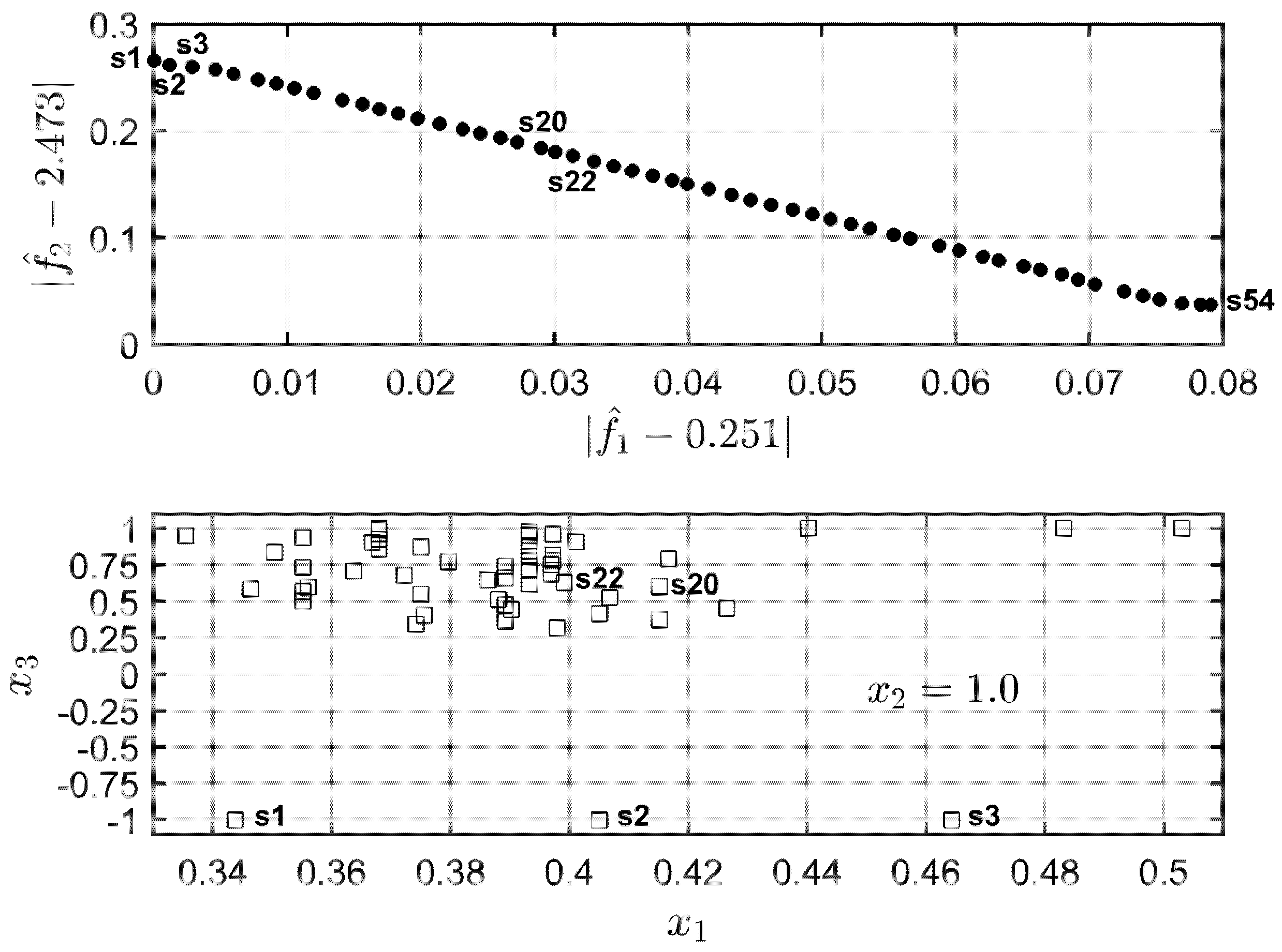
According to the steps 1–2 of the proposed approach-implementation procedure presented in 2.4, optimal solutions were generated using ${\widehat{f}}_1(\mathbf{x})$ and ${\widehat{f}}_2(\mathbf{x})$ as objective functions, which were equally weighted (${\omega }_1={\omega }_2=1/2$). Both the carotenoid and chlorophyll extractions are larger-the-better-type responses. 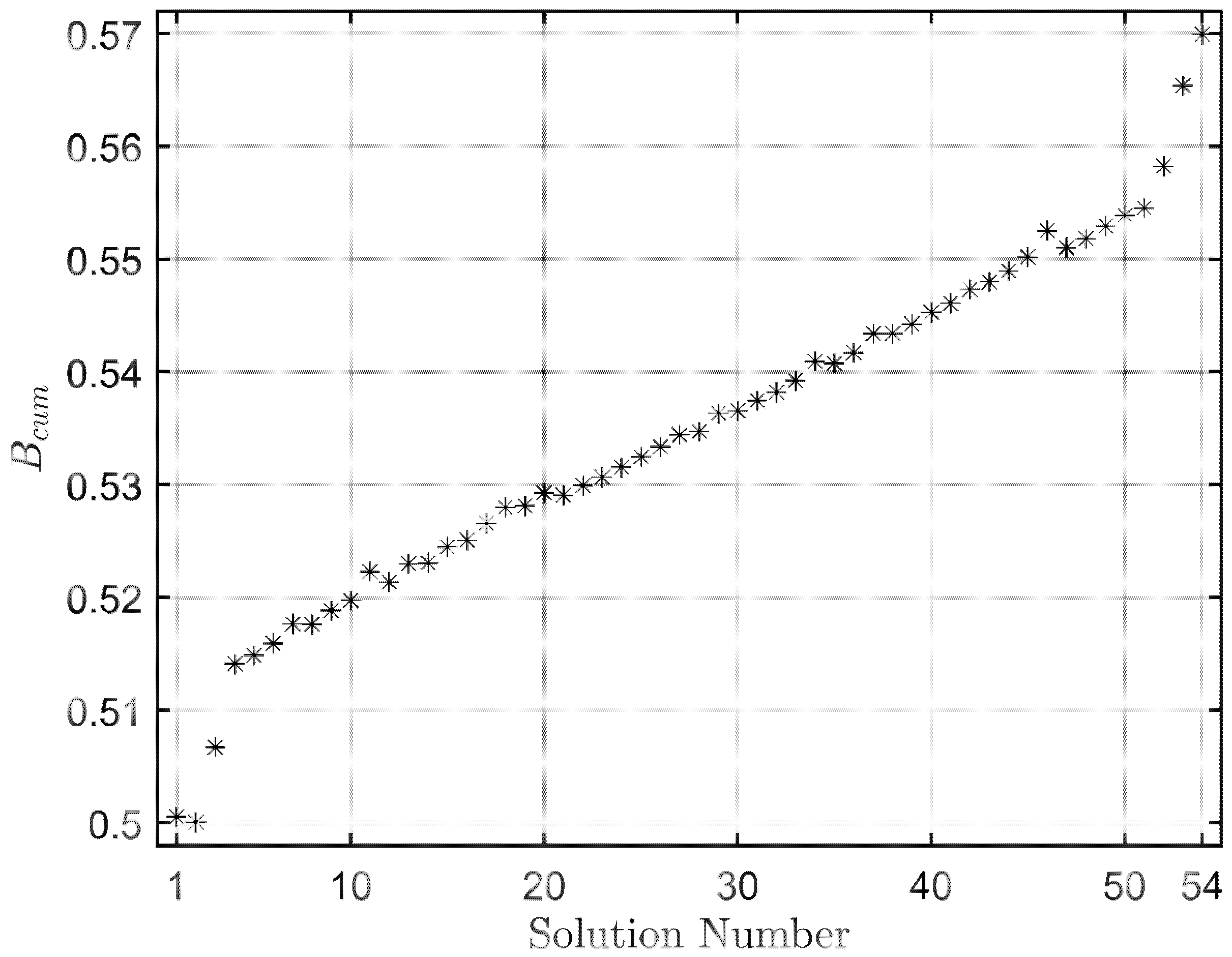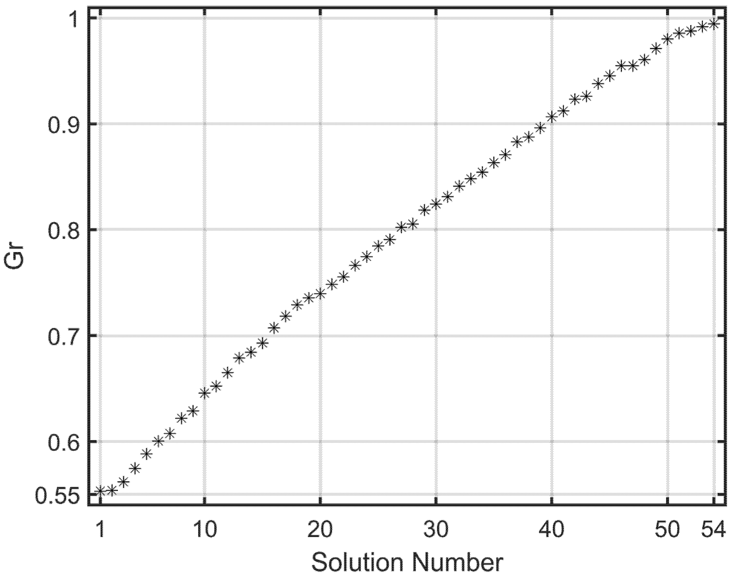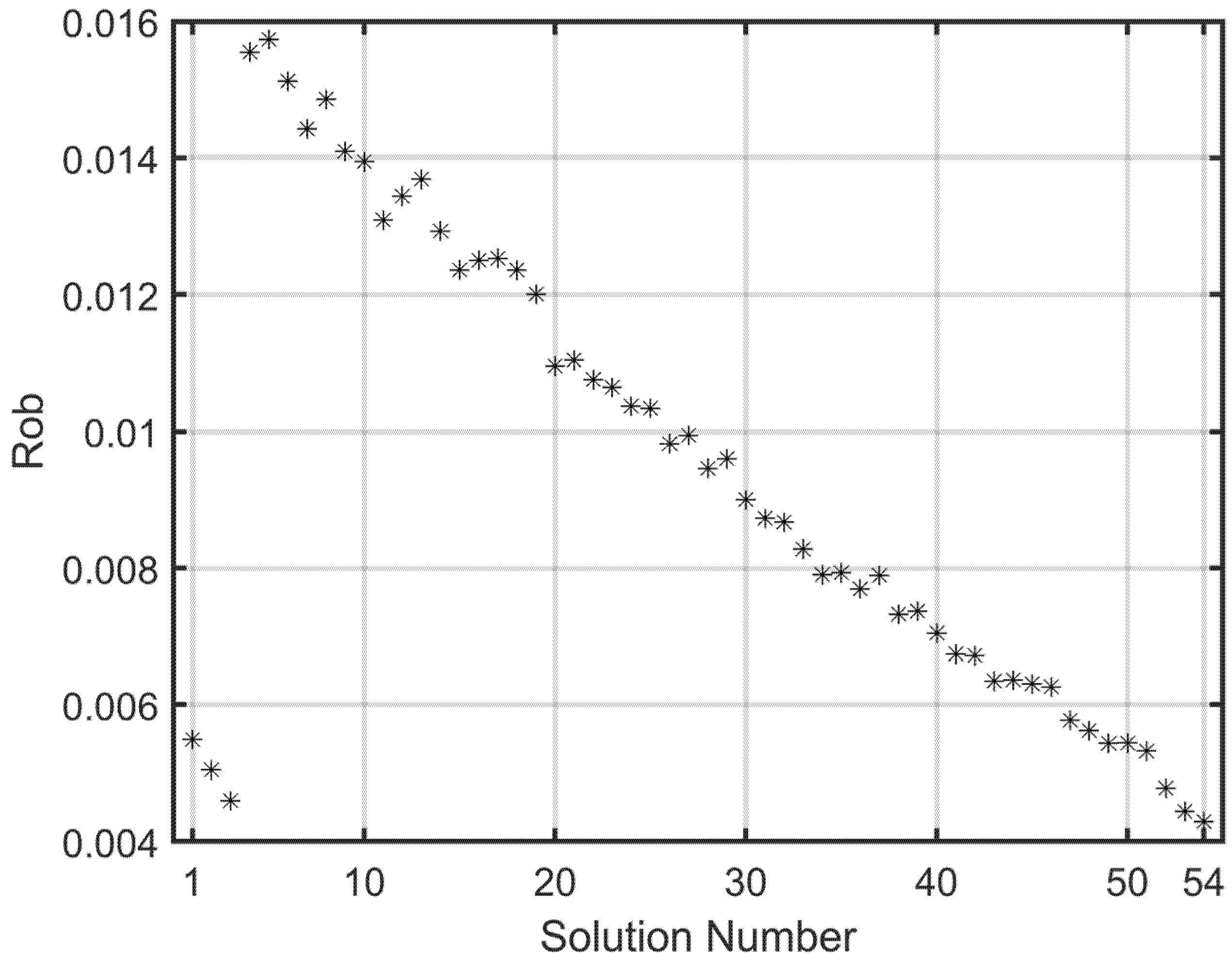The generated Pareto set, which has 54 solutions, is shown in Figure 1. With these data, the solution’s properties, $B_{cum}$ (32), $Gr$ (33), Rob (35), and $QoP$ (36), were calculated. 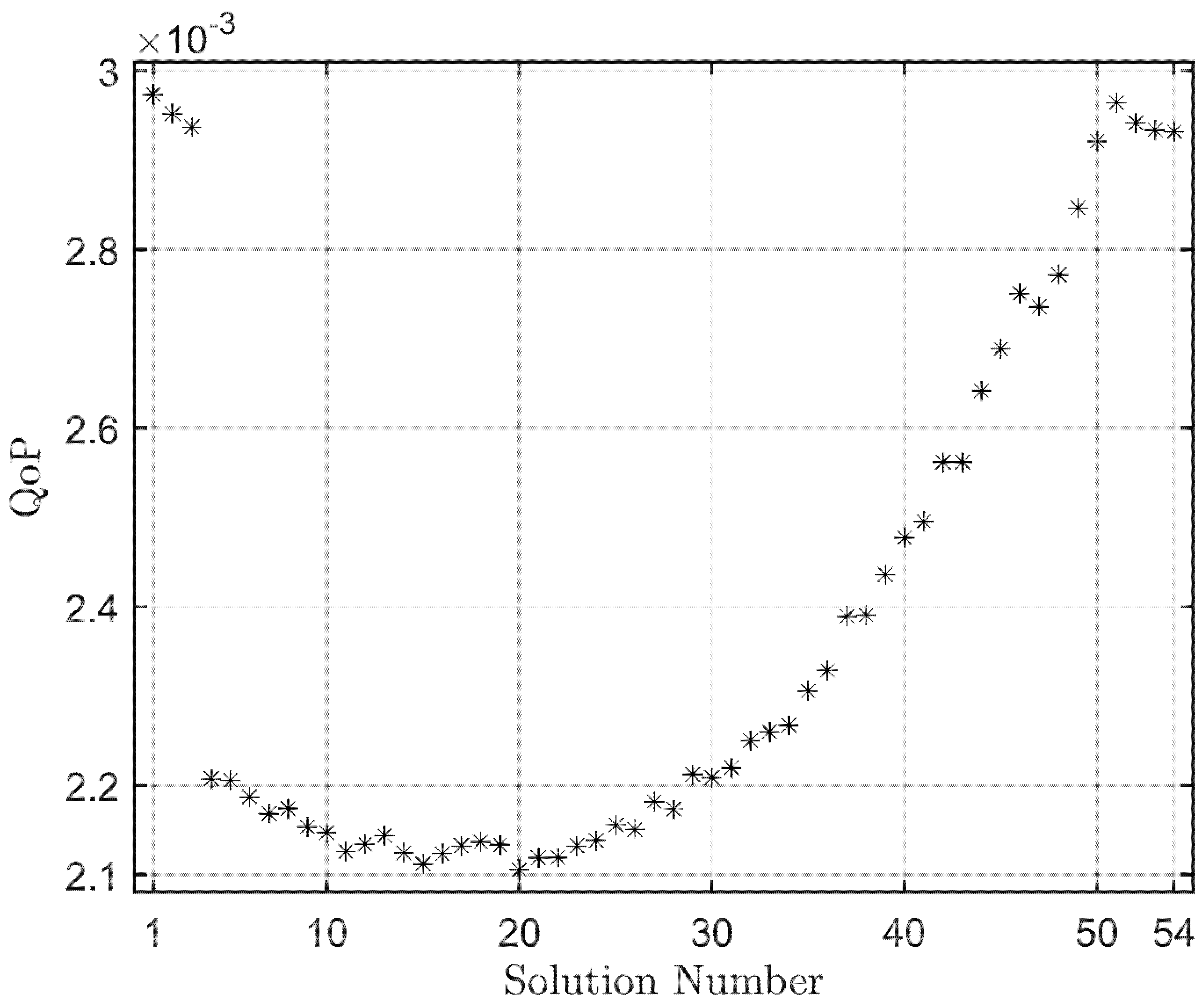Their values are shown in Figure 2, Figure 3, Figure 4 and Figure 5. As can be seen from these figures, the solutions with the best values for $B_{cum}$ (32), $Gr$ (33), Rob (35), and $QoP$ (36) are S2, S20, S54, and S1, respectively. Since no single solution satisfies all four properties simultaneously, the “best” solution must therefore represent a trade-off among them.

For weighing the solution properties (Step 4 of the proposed approach), twenty sets of weights were generated to account for uncertainty in the decision-maker’s specification of the weight values. It was assumed that, in the absence of any technical or economic justification, the weights assigned to the solution properties are $\left(w_B^0,w_Q^0,w_G^0,w_R^0)=(1/4, 1/4, 1/4, 1/4\right)$. A variation of 10% around these baseline values $\left(\vartheta =0.1\right)$ is considered appropriate to account for the uncertainty in the weight values. Thus, each weight $w_i^0$ will vary within the interval $\left[\hspace{0.17em}{w}_i^0(1-\vartheta ), w_i^0(1+\vartheta )\hspace{0.17em}\right]$, while satisfying the condition ${\sum }_i{w}_i=1$.

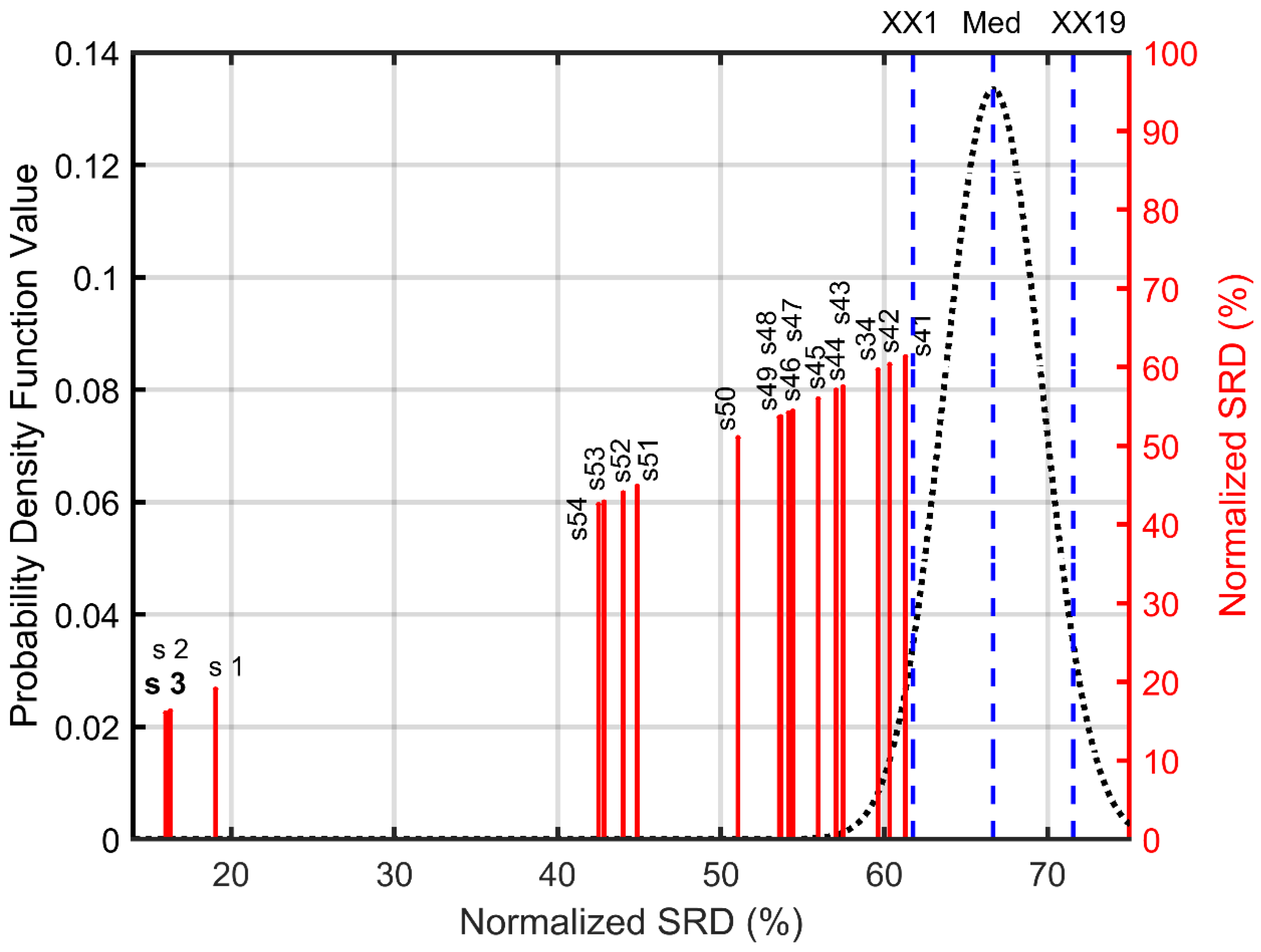
The 10 MADM methods presented in Section 2.1 were applied to evaluate the pareto solutions (Step 6 of the proposed approach), using as input the property values ($B_{cum}$ (32), $Gr$ (33), Rob (35), and $QoP$ (36)) associated with each solution. The SRD analysis (steps 7–8) was then performed on a $200\times 54$ matrix, where the columns represent the optimal solutions under comparison, while the rows correspond to the evaluation obtained from applying the 10 MADM methods to the same set of solutions using 20 weight sets (step 6). The results of the SRD-CRRN analysis are shown in Figure 6 (step 9). 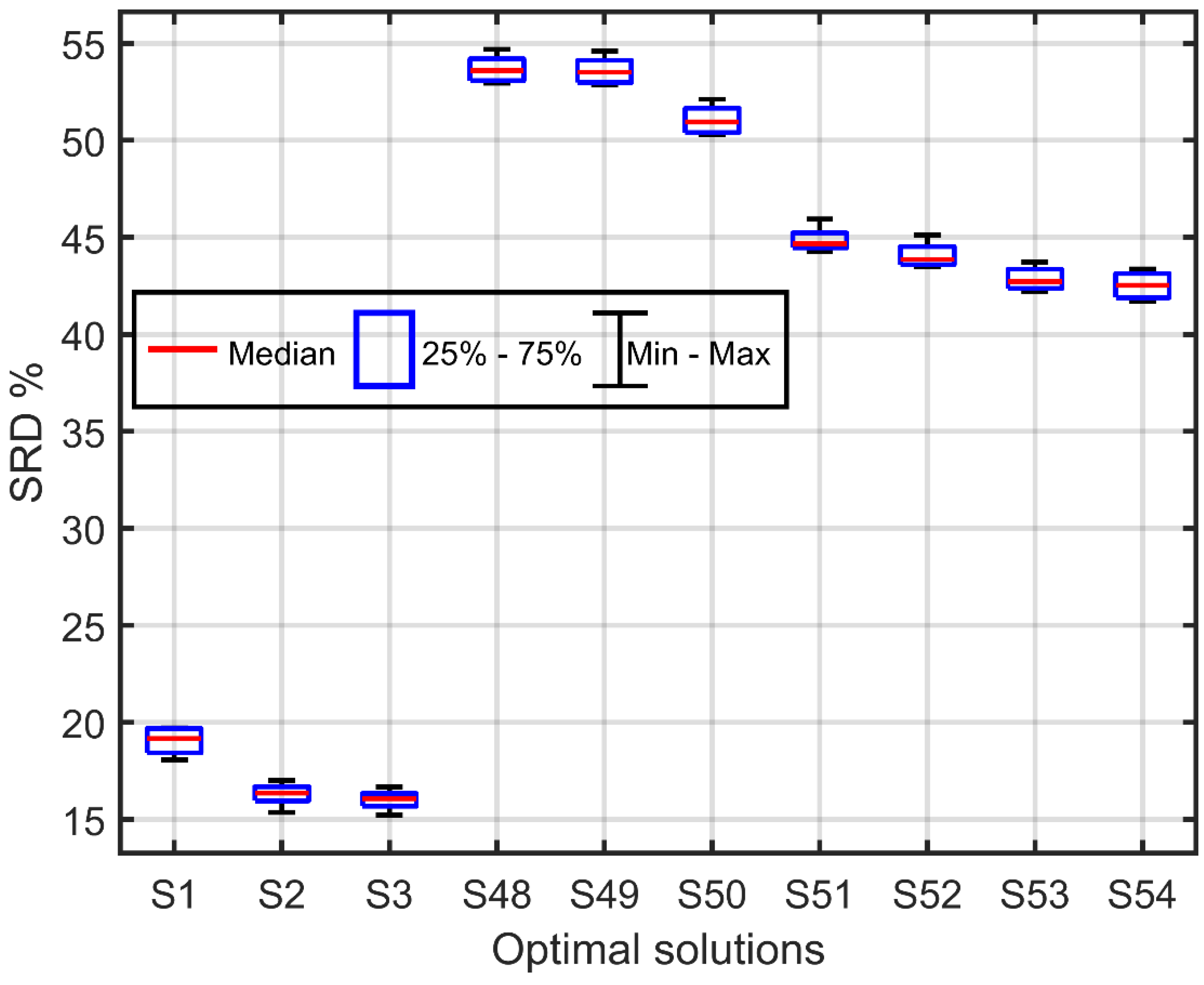The analysis suggests that the best solutions, those with an SRD value closest to zero, are S3 and S2 (see Figure 6). Solutions S1, S54, S53, S52, S51, S50, S49, S48, S46, S47, S45, S44, S43, S34, S42, and S41 are also below the 5% significance threshold, indicated by the dashed XX1 line, which means they also differ from random ranking. To evaluate the uncertainty associated with the SRD results, eight-fold cross-validations (CV) were conducted. The box-and-whisker plot presented in Figure 7 suggests no differences between solutions S2 and S3, whereas S1 differs from both. These outcomes are confirmed at 5% significance level by the Wilcoxon test, the 10-fold Alpaydin test, and the 10-fold Dietterich test. It is important to note that these three solutions are very similar in terms of bias, prediction quality, resilience, and robustness values, as shown in Figure 2, Figure 3, Figure 4 and Figure 5. However, several methods penalized solution S1 more severely than the other two solutions, as it exhibits the worst QoP (36) value. In fact, out of the 200 evaluations performed (20 weight sets × 10 MADM methods), S3 was selected as the best solution 80 times, S2 was selected 72 times, and S1 was never selected. To conclude this analysis, which considers the four properties equally, the results obtained confirm expectations: solutions S1, S2, and S3 are the three best solutions in terms of $B_{cum}$ (32), $Gr$ (33), and are among the top nine according to Rob (35), even though they rank among the worst for $QoP$ (36).

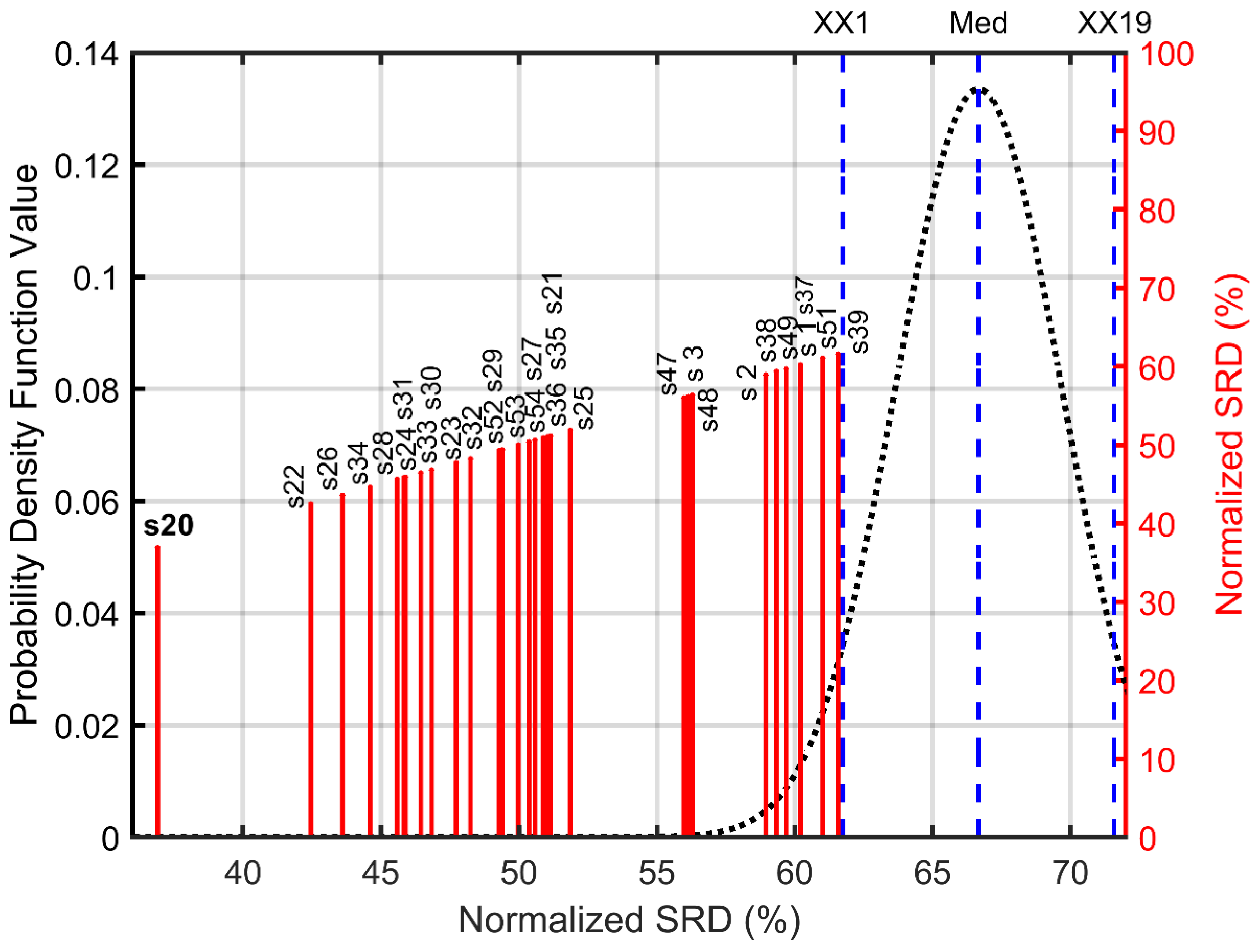
Another evaluation of the Pareto set was performed using new 20 weight sets. The nominal weight values and the allowed variation were $\left(w_B^0, w_Q^0, w_G^0, w_R^0\right)=\left(1/6, 1/2, 1/6, 1/6\right)$ and $\vartheta =10\%$, respectively. This choice of weights assumed that the decision-maker places particular emphasis on prediction quality, with a 10% degree of uncertainty in the stated preferences. 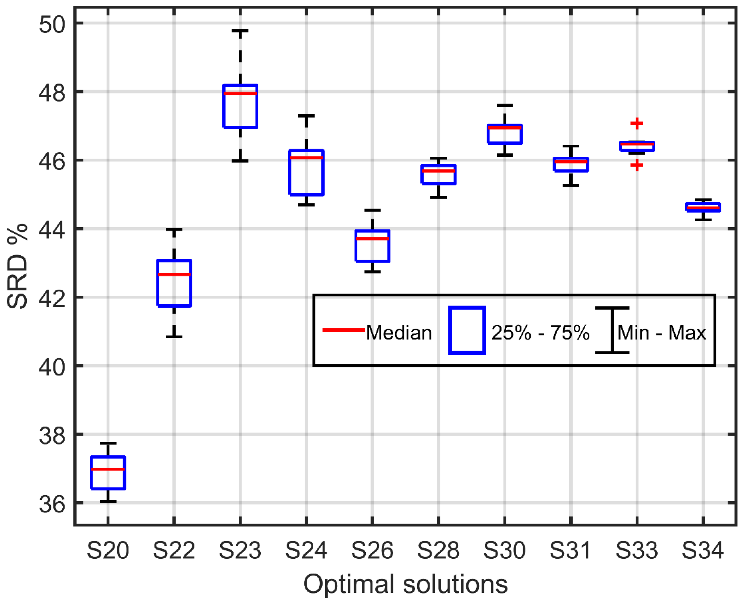According to the SRD-CRRN results presented in Figure 8, several solutions outperform the random ranking, as they fall to the left of the 5th percentile threshold (XX1 line). However, the same figure indicates that solution S20, performs better than the other solutions. An eight-fold cross-validation was also performed to assess the uncertainty of the SRD results. The box-and-whisker plot (Figure 9) indicates relevant differences between solution S20 and all the other solutions. These differences are confirmed at 5% significance level by the Wilcoxon test. However, the 10-fold Alpaydin, and the 10-fold Dietterich tests do not support a significant difference between S20 and S22. This difference between the test results is justified by the higher fluctuation of SRD values under the Alpaydin and Dietterich tests than under the Wilcoxon test, due to the cross-validation methods they employ. While Wilcoxon’s k-fold approach removes only a fraction of rows (m/k) per fold, Alpaydin and Dietterich tests remove half the data (50%) in each iteration, leading to higher variance [24,55]. An analysis of Figure 2, Figure 3, Figure 4 and Figure 5 and

Table 4. Optimal solutions—Properties.

Solution	${\mathit{x}}_1$	${\mathit{x}}_2$	${\mathit{x}}_3$	${\widehat{\mathit{f}}}_1(\mathbf{x})$	${\widehat{\mathit{f}}}_2(\mathbf{x})$	${\mathit{B}}_{\mathit{c}\mathit{u}\mathit{m}}$	$\mathit{Q}\mathit{o}\mathit{P}$	$\mathit{G}\mathit{r}$	$\mathit{R}\mathit{o}\mathit{b}$
S1	0.344	1	−1	0.251	2.207	0.5006	0.0029	0.5531	0.0055
S2	0.405	1	−1	0.25	2.211	0.5001	0.0029	0.5539	0.0050
S3	0.464	1	−1	0.248	2.214	0.5067	0.0029	0.5618	0.0046
S20	0.415	1	0.602	0.222	2.289	0.5293	0.0021	0.7397	0.0110
S22	0.399	1	0.630	0.22	2.297	0.530	0.0021	0.7555	0.0108

also shows that solution S20 presents better bias ($B_{cum})$, prediction quality ($QoP)$, and resilience ($Gr$) values than S22, which is the solution closer to S20 in Figure 8. Therefore, considering that S20 was selected as the best solution 79 times in 200 compared to 0 for S22, one can assume that S20 is the most favorable solution (best choice). Once again, these results confirm expectations: solution S20 is the best according to the QoP property (see Figure 3), which has the highest nominal weight ($w_Q^0=0.5)$. Regarding the remaining three properties, which are all equally weighted (${\mathrm{w}}_B^0={\mathrm{w}}_G^0={\mathrm{w}}_R^0=1/6$), S20 ranks 20th out of 54 for both resilience ($G_r$) and bias ($B_{cum}$), while for $R_{ob}$ it is the 18th worst solution. Overall, this indicates that S20 represents a well-balanced solution with respect to the chosen weights.

With regard to the solutions chosen by each MADM, for $\left(w_B^0, w_Q^0, w_G^0,w_R^0\right)=\left(1/4, 1/4, 1/4, 1/4\right)$, among 54 optimal solutions, 8 were selected by the 10 MADM methods used, whereas for $\left(w_B^0, w_Q^0, w_G^0,w_R^0\right)=\left(1/6, 1/2, 1/6, 1/6\right),$ 6 solutions were selected. Of these last six solutions, three differ from those obtained with the other set of weights. It is also important to highlight that among the 10 MADM methods used, four selected the same solutions, showing variability in the solutions identified by the MADM methods. Only three methods (WASPAS, MOORA, and TOPSIS_N) selected the solution statistically more favorable for both weighting schemes. These results confirm, on the one hand, the diversity in the selection of the best solutions by the ten used methods and, on the other hand, the proposed approach sensitivity to changes in properties’ weight (i.e., decision-makers’ preferences).

4. Conclusions

Organizations’ sustainability is nowadays a strategic element of competitive differentiation, so operations efficiency, namely the process and product improvement, innovation, and socio-environmental responsibility, are key drivers for value creation in business management. To ensure long-term sustainability, decision-makers in industrial and non-industrial settings often need to solve problems where a compromise between multiple conflicting criteria is required. Therefore, the decision-making process must be supported on multiple attribute or multiple objective decision-making methodologies, methods, procedures, and techniques that enable the creation of a scientifically robust decision-making framework where it is possible to balance economic, environmental, and social factors. In multi-objective optimization, selecting a solution from the Pareto set is not an irrelevant task due to its impact on process and/or product and, consequently, on one or more sustainability’s dimensions. When Pareto optimal solution properties are considered in the evaluation of these solutions, the decision-maker faces a multi-attribute problem, which means that the solution selection for this problem must be supported on appropriate multi-attribute methods, on an empirical or expert sensitivity basis. However, the quantity and variety of existing methods made method selection difficult for those who need to solve a multi-attribute problem. On the one hand, one cannot expect that those who need to solve multi-attribute problems have the required statistical background and access to the literature for selecting the most appropriate analysis method(s); on the other hand, no method can be considered superior to all others in every situation. Ranking the solutions selected by the methods is a difficult task so a procedure to rank solutions fairly is a need and a useful contribution for better decisions in problems with conflicting attributes. The SRD technique has proven to be effective, so it was used to identify the most favorable optimal solution. In this paper, this technique was integrated into a structured approach, where ten MADM methods were used to select optimal solutions, and its usefulness was illustrated in a problem where the identified Pareto solution should yield the most favorable value for bias, quality of prediction, and resilience and robustness, and this way to ensure better reproducibility for the generated Pareto solutions. In fact, some optimal solutions may not be an option to implement in the process and/or product, due to time, cost, and other technical constraints, namely the lack of solutions reproducibility. Therefore, the solutions reproducibility is imperative and a major concern in the proposed approach for sustainability improvement.

The accuracy of the input data, namely, the attribute-weighting process, also significantly influences the effectiveness of MADM methods. Thus, the proposed approach suggests that sets of weights must be defined to incorporate the decision-maker’s uncertainty in specifying those weights. This is relevant because weight values significantly impact the outcome of the decision-making process. Therefore, in the proposed approach, a well-distributed coverage of weight space within the variation interval specified to them is suggested, which reinforces the validity of the results presented.

The presented proposal addresses the balance between solutions with higher reproducibility and solutions where reproducibility is not considered (only the Bias is minimized). It proved its usefulness in a case study from the literature, however, other case studies from different science fields can be used to confirm its usefulness and democratize its use. Other MADM methods can be also tested, though subjective information is always required from the user/decision-maker. In addition, an alternative to SRD is also possible, as this technique is not easy to interpret and/or apply, even with the available software to implement it. An online platform to test the proposed approach is also planned.