


Abstract
This study proposes a reproducible methodology for optimizing occupancy sensor placement and assessing the sustainable energy performance of smart lighting systems in university classrooms. The research was conducted in Block H of the South Campus of the Universidad Politécnica Salesiana, Quito, using one representative classroom for detailed geometric analysis and extending the optimization to eight classrooms with different dimensions, areas, and installed lighting configurations. The proposed framework integrates Voronoi-based spatial analysis, genetic algorithm optimization, and dynamic occupancy-based lighting control simulation as a retrofit-oriented strategy for existing educational buildings. For the representative classroom, the optimized sensor position was located near the geometric center of the room and achieved an estimated spatial coverage of 94.7% under the adopted sampling-based geometric model and an effective detection radius of 6 m. The multi-classroom analysis showed that the required number of sensors depends on classroom geometry and the adopted sensing radius; at R = 6 m, most classrooms satisfied the 90% coverage criterion with one sensor, while the largest classroom required two sensors. Based on occupancy schedules and automatic control rules, the dynamic simulation showed reductions in lighting operating time of 48% and 52% for 10 h and 12 h daily scenarios, respectively. These reductions were translated into lower daily and monthly energy consumption across different lighting configurations. The results indicate that optimized occupancy-based control can support sustainability-oriented energy management in university buildings by reducing unnecessary electricity use while preserving the existing lighting infrastructure. However, the results are limited to occupancy-based control and do not include daylight harvesting, photometric validation, or a complete economic payback assessment.
1. Introduction
Lighting systems represent an important component of electricity consumption in educational buildings, particularly in classrooms with long daily operating periods and intermittent occupancy. From a sustainability perspective, reducing unnecessary lighting operation in existing university buildings is a practical way to improve energy efficiency, decrease avoidable electricity demand, and support more responsible campus energy management without requiring complete infrastructure replacement. In many university facilities, luminaires remain switched on during vacant periods because lighting operation depends mainly on manual switching or fixed schedules. This situation creates an opportunity for control-oriented sustainability measures that can improve building performance through intelligent operation rather than through major construction or replacement interventions. Occupancy-based lighting control is especially relevant in this context because it can reduce unnecessary operating time by linking lighting operation to actual or assumed room use. However, the effectiveness of this strategy depends not only on the control rule itself, but also on the spatial placement of the occupancy sensor, the sensing radius, the classroom geometry, and the operating schedule considered in the simulation.
The main contribution of this study is the development of a reproducible framework for the placement of occupancy sensors and the evaluation of sustainable energy performance in smart lighting systems for university classrooms. The framework integrates Voronoi-based spatial analysis, genetic algorithm optimization, and dynamic occupancy-based control simulation. Its application to an existing educational building shows that sensor-based control can reduce lighting operating time and improve energy performance without modifying the installed lighting layout. In this context, the sustainability contribution of the study lies in providing a practical decision-support framework for reducing lighting energy waste in existing educational buildings. Rather than proposing a complete lighting redesign, the approach focuses on optimizing the use of the installed infrastructure through sensor placement, occupancy-based control, and energy-performance indicators. This makes the methodology especially relevant for university campuses where retrofit-oriented actions are often more feasible than large-scale replacement projects.
1.1. State of the Art
Recent research on smart lighting in buildings can be grouped into three main strands: (i) occupancy- or presence-based lighting control in educational environments, (ii) optimization-oriented sensor placement methods, and (iii) lighting control studies with explicit energy performance assessment. These strands provide the methodological and application background for developing a reproducible framework for occupancy sensor placement and energy assessment in existing university classrooms.
In educational buildings, several studies have shown that occupancy-based lighting control can substantially reduce unnecessary operating time and electricity use. Seo and Yun developed a digital-twin-based assessment framework for university classroom lighting and reported that lights remained on without occupants for an average of 10.7 h/day. Their results showed that PIR-based on/off control achieved weekly energy savings of approximately 63–64%, while combined control strategies reached savings of about 80–81% [1]. These findings confirm that occupancy-driven control is a relevant strategy for reducing lighting energy consumption in academic buildings.
Additional evidence from educational environments shows that the effectiveness of sensor-based lighting control depends not only on the presence of sensors but also on control parameters and user interaction. Myshonkov and Atishev reported that motion-sensor-based on/off control in a public educational building achieved average savings of at least 50%, while longer switch-off delays reduced the savings from 66.5% to 48.5%, and standby lighting reduced them further to 21.9% [2]. Likewise, Karaman Madan and Pekeriçli highlighted that user acceptance is a relevant practical constraint, showing that conventional occupancy-sensor strategies were not always well perceived, whereas a more user-centric control approach improved acceptance while maintaining the energy-saving potential [3]. Together, these studies indicate that realistic control rules and user-oriented operation should be considered when evaluating intelligent lighting systems in university buildings.
Other recent works have explored smart lighting implementations in academic environments through Internet of Things (IoT) architectures and sensor-assisted automation. For example, González-Amarillo et al. developed an IoT-based smart lighting system for academic environments using chair-mounted infrared presence sensors, photocells, and web-based monitoring, reporting energy savings above 60% in a university laboratory/classroom case study [4]. Although this type of approach demonstrates the feasibility of occupancy-aware smart lighting in educational spaces, the sensing strategy is often embedded in furniture or in a specific hardware configuration, which limits transferability to conventional retrofit scenarios in existing classrooms. In a related optimization-oriented IoT study, Obioma et al. proposed a smart lighting system integrating occupancy and presence sensors together with illuminance sensing and constrained dimming optimization, showing that optimization-based control can produce substantial power savings, although the study focused on office environments and luminaire-integrated sensing rather than on sensor placement in classrooms [5].
In parallel, a substantial part of the recent optimization literature has focused on the placement of illuminance sensors rather than occupancy sensors. Wagiman et al. proposed an optimal light sensor placement method based on an illuminance-center-grid model and particle swarm optimization, reporting energy savings of up to 24.5% while satisfying the standard [6] EN 12464-1 illuminance and uniformity requirements [7]. More recently, Feyzi and Mojallali presented an optimization method for light sensor placement in smart buildings under illuminance and uniformity constraints, reporting energy savings of up to 30.8% together with acceptable visual comfort conditions [8]. These studies are methodologically relevant because they demonstrate how geometric candidate locations, optimization algorithms, and lighting-performance constraints can be integrated into a reproducible workflow. However, their main focus is on illuminance sensing for dimming control rather than on occupancy or presence sensor placement.
Beyond lighting-specific applications, recent work on occupancy sensor deployment has shown that spatial optimization itself can be formulated explicitly as a geometric problem. Lu and Radke proposed an automatic occupancy sensor placement method for smart environments using simulated occupant trajectories and integer linear programming, showing that sensor layout can be optimized systematically instead of being selected through manual trial and error [9]. From a broader lighting-controls perspective, previous review and meta-analysis studies also show that energy savings depend strongly on the type of control, the occupancy pattern, the commissioning strategy, and the acceptance of users. De Bakker et al. reviewed occupancy-based lighting control in open-plan offices and emphasized that this strategy may reduce lighting energy use, but that further validation is needed regarding cost-effectiveness, user acceptance, and real operating conditions [10]. Similarly, Williams et al. analyzed 240 lighting-control savings estimates from 88 studies and reported average savings of 24% for occupancy-based control, 28% for daylighting, and 38% for combined control strategies [11]. These findings are relevant to the present study because they show that occupancy sensing should not be evaluated only as a hardware intervention, but also as a control strategy whose performance depends on the installation context, operating schedule, and implementation cost.
Although the study by Lu and Radke did not evaluate lighting energy performance and was developed for office-like environments, it is methodologically relevant because it reinforces the need to connect geometry-based sensor deployment with application-specific performance metrics.
Therefore, the current literature provides strong evidence that occupancy-based control can improve the energy performance of lighting systems in educational buildings and that optimization methods can support sensor deployment in indoor environments. However, these two research lines are still largely disconnected. Studies conducted in university classrooms generally evaluate occupancy-based control as a scenario or operating strategy, but they do not explicitly optimize sensor location as a geometric coverage problem. Conversely, studies on sensor placement optimization are mostly centered on illuminance sensors and visual comfort criteria rather than on occupancy detection and its impact on lighting operating time and energy use [1,7,8,9]. This reveals the need for a reproducible framework that explicitly links spatial analysis of sensor coverage, optimization of occupancy sensor placement, dynamic occupancy-based control simulation, and energy performance indicators in existing university classrooms. Recent bibliometric evidence also supports the relevance of integrating human-centric control, IoT platforms, and automation-related optimization in smart indoor lighting research. Tipán et al. [12] showed that smart lighting studies increasingly connect energy efficiency, occupant-centered control, automation frameworks, and interoperable IoT platforms. This broader perspective reinforces the need for applied methodologies that translate these research trends into reproducible design-support tools for existing educational buildings, as summarized in Table 1.
Table 1.
Comparison between related studies and the proposed framework.
1.2. Research Gap and Contribution
Although recent studies have demonstrated that occupancy-based lighting control can significantly reduce electricity consumption in educational buildings, important limitations remain in the current literature. First, most classroom-oriented studies assess occupancy-based control as an operational scenario, but they do not formulate sensor location as an explicit optimization problem based on spatial coverage and retrofit constraints. Second, the majority of optimization-oriented studies focus on illuminance sensor placement and daylight-linked dimming strategies, rather than on occupancy or presence sensor deployment for lighting control in existing classrooms. Third, even when energy savings are quantified, geometric sensor coverage, control-rule dynamics, and energy indicators are rarely integrated into a single reproducible workflow applicable to educational buildings.
Therefore, there is still a need for a practical and reproducible framework that explicitly connects spatial analysis of occupancy sensor coverage, optimization of sensor placement, dynamic simulation of lighting control, and energy performance assessment in existing university classrooms. Such a framework is particularly relevant in retrofit-oriented scenarios, where the installed lighting layout remains unchanged and the improvement strategy relies on intelligent control rather than on redesigning the luminaires.
To address this gap, this study proposes an integrated methodology for optimizing occupancy sensor placement and assessing its effect on the energy performance of smart lighting systems in university classrooms. The proposed framework combines Voronoi-based spatial analysis for preliminary coverage assessment, genetic algorithm optimization for determining sensor location, and dynamic occupancy-based simulation for estimating lighting operating time and electricity consumption. In this way, the study links geometric optimization with energy assessment while preserving the existing lighting infrastructure.
The main contribution of this work is the development of a reproducible framework for evaluating occupancy-based smart lighting control in educational buildings through spatial coverage and energy performance indicators. In addition, the study provides quantitative evidence of the potential of optimal occupancy sensor placement to reduce lighting operating time and energy consumption in university classrooms without modifying the installed lighting layout. In addition, practical deployment requires attention to the number of sensors, installation effort, commissioning, and compatibility with the installed luminaire technology. In this study, the number of sensors required to satisfy a minimum coverage criterion was used as a practical proxy for hardware complexity. A full monetary cost–benefit analysis was not performed because local sensor prices, installation labor costs, commissioning costs, electricity tariffs, and maintenance records were not available as validated input data. Therefore, the economic interpretation is treated as a reproducible screening step rather than as a quantified payback result.
The aim of this study is to optimize the placement of occupancy sensors and evaluate their impact on the energy performance of smart lighting systems in university classrooms. For this purpose, the proposed methodology is applied to Block H of the South Campus of the Universidad Politécnica Salesiana, Quito, as a representative case study of an existing educational building. The remainder of this paper is organized as follows. Section 2 presents the materials and methods, including the spatial analysis, the optimization framework, the dynamic simulation model, and the energy indicators. Section 3 describes the case study and discusses the main results. Finally, Section 4 summarizes the main conclusions and outlines future research directions.
2. Materials and Methods
2.1. Overall Methodological Framework
The methodological framework adopted in this study was designed to evaluate the effect of occupancy sensor placement on the energy performance of smart lighting systems in existing university classrooms. The approach combines spatial analysis, heuristic optimization, dynamic control simulation, and energy indicator assessment in a single workflow. The objective was not to redesign the installed lighting system, but rather to improve its operational efficiency through occupancy-based control while preserving the existing luminaires and layout. The input data used in the framework were separated into measured or documented information and modeling assumptions. The architectural and electrical data, including classroom dimensions, lighting layout, number of luminaires, and installed lighting power, were obtained from the available floor plans and lighting inventory of Block H. In contrast, the occupancy schedules used in the dynamic simulation were not obtained from continuous data logging or automated occupancy measurements. They were defined as representative academic-use schedules based on the regular operating window of the classrooms and the project assumptions adopted for the case study. Similarly, the baseline lighting-use pattern was modeled as continuous manual operation during the considered academic-use period, rather than as a measured time series of actual switching events. This distinction is important because the resulting energy savings should be interpreted as simulation-based estimates under representative operating assumptions, not as directly monitored post-retrofit savings.
The methodology was applied to Block H of the South Campus of the Universidad Politécnica Salesiana, Quito, which is composed of classrooms with similar geometric characteristics, comparable lighting layouts, and recurrent academic occupancy patterns. This condition made it possible to define a representative classroom for detailed spatial analysis and optimization, while enabling the extension of the optimization procedure to multiple classrooms in the same block under common methodological assumptions.
The first stage of the methodology consisted of gathering the architectural and electrical information of the study area, including classroom dimensions, installed lighting power, number of luminaires, and typical operating schedules. Based on this information, the floor plans were processed in a two-dimensional Cartesian geometric model to obtain a scaled representation of the classroom and to delimit the useful area for analysis.
In the second stage, a Voronoi-based spatial analysis was performed to obtain an initial interpretation of sensor influence zones within the classroom. This procedure allowed the space to be partitioned into regions associated with preliminary sensor locations, facilitating the identification of more balanced and spatially coherent candidate areas. The Voronoi analysis was used as an exploratory geometric tool to support the subsequent optimization stage rather than as a final decision mechanism by itself.
In the third stage, a genetic algorithm was implemented to determine the optimal occupancy sensor location inside the selected classroom. Each candidate solution was represented by the sensor coordinates in the two-dimensional classroom plane. The optimization process was guided by a multi-criteria fitness function that prioritized spatial coverage, incorporated a geometric regularization term based on average distance to sampling points, and included an indirect energy-related penalty associated with uncovered zones. In this way, the optimization stage connected geometric sensor placement with the expected operational behavior of the lighting control system.
The fourth stage consisted of a dynamic simulation of the lighting control logic under occupancy-based operation. The simulation was performed with a one-minute temporal resolution and considered representative daily schedules of 10 h and 12 h. A binary occupancy model was used to represent classroom use, and the control logic was defined by three rules: automatic switch-on when occupancy was detected, maintenance of the ON state during a delay period after vacancy, and automatic switch-off once the delay elapsed. The delay time was fixed at 5 min in order to represent a realistic commercial control strategy.
Finally, the last stage of the methodology focused on energy performance assessment through a set of quantitative indicators. These indicators included current energy consumption, energy consumption with occupancy sensors, energy savings, lighting power density, power per occupant, and energy consumption per unit area. The comparison between the baseline condition and the proposed controlled condition allowed the impact of the optimized sensor placement to be expressed in operational and energy terms.
Overall, the proposed framework establishes a reproducible route from geometric classroom characterization to energy-performance evaluation. Its main strength lies in linking occupancy sensor placement with dynamic lighting operation in existing educational spaces, thus providing a practical methodology for improving lighting efficiency without modifying the installed lighting infrastructure.
As shown in Figure 1, the proposed methodology is not limited to a linear sequence of tasks. Each stage produces an explicit output that is used in the next step: the geometric model defines the sampling points, the Voronoi analysis supports the initial interpretation of candidate regions, the genetic algorithm provides the optimized sensor configuration, the dynamic simulation converts occupancy detection into effective lighting operating time, and the energy assessment translates this operating time into performance indicators.
Figure 1.
Detailed methodological framework adopted for occupancy sensor placement optimization and energy performance assessment. The workflow identifies the input data, the main processing stages, and the outputs generated at each stage, linking geometric modeling, spatial analysis, genetic algorithm optimization, dynamic control simulation, and energy indicators.
2.2. Case Study Description
The case study corresponds to Block H of the South Campus of the Universidad Politécnica Salesiana, Quito, Ecuador. This block is composed of academic spaces with frequent daily use, mainly classrooms devoted to teaching and meeting activities. Because of their recurrent occupancy and prolonged operating schedules, these spaces represent a relevant scenario for evaluating the potential of occupancy-based lighting control to improve energy efficiency. Block H was selected because it combines several characteristics that are relevant for evaluating occupancy-based lighting control in an existing educational building: recurrent classroom use, prolonged academic operating periods, available architectural and electrical documentation, and multiple lighting configurations within the same block. These conditions made it possible to test the proposed workflow under a controlled but realistic retrofit-oriented context. The building was not selected to statistically represent all buildings on campus or all educational facilities. Rather, it was used as a case study of a typical university classroom environment in which lighting operation depends strongly on academic occupancy patterns and where modifying the lighting layout is not the primary intervention. Therefore, the findings are generalizable mainly at the methodological level: the proposed workflow can be transferred to other classrooms or buildings if equivalent geometric, electrical, and occupancy information is available. Quantitative results such as coverage, number of sensors, and energy savings should be recalculated for each new building because they depend on room geometry, sensor characteristics, luminaire technology, and actual occupancy schedules.
Among the spaces identified in Block H, eight classrooms with regular academic use and suitable geometric definition were included in the multi-classroom optimization analysis.
The geometric characteristics of the classrooms included in the multi-classroom analysis are summarized in Table 2. These dimensions were used to define the feasible search domain of the optimization problem and to support the comparison of sensor placement results across the analyzed classrooms.
Table 2.
Geometric characteristics of the classrooms analyzed in Block H.
The operating schedules of the classrooms extend throughout the academic day, from 07:00 to 21:00, which increases the relevance of control-oriented energy-saving measures. From the spatial and operational perspective, this block provides favorable conditions for evaluating the interaction between classroom geometry, occupancy behavior, sensor coverage, and lighting energy use. The 07:00–21:00 interval corresponds to the normal weekday academic operating window considered for Block H in this study. This time range was used to define the maximum daily availability of the classrooms; however, the dynamic simulations were performed for 10 h and 12 h representative daily scenarios to avoid assuming continuous full-day occupation. Exceptional periods such as weekends, holidays, examination weeks, or special events were not modeled separately. Therefore, the results should be interpreted as representative of regular academic operation rather than as a complete annual occupancy model.
For the methodological development, one representative classroom was selected for detailed spatial analysis and optimization. The selection was based on geometric regularity, representativeness within the block, and its suitability for illustrating the complete geometric and optimization workflow adopted in the study.
In addition, the block includes different lighting configurations, including 32 W fluorescent ballast-based luminaires, 60 W LED luminaires, and 18 W LED luminaires, which allowed the analysis to include several operational scenarios in the energy assessment stage.
These lighting technologies were not assumed to respond identically from a maintenance perspective. The energy calculations compare the reduction in operating time for each installed power scenario, but they do not include lamp degradation, ballast aging, replacement cost, or maintenance cost. For this reason, the ballast-based fluorescent scenarios should be interpreted with additional caution when applying short-delay ON/OFF control, whereas the LED scenarios are more directly compatible with frequent switching and future dimming-based control strategies.
The case study was therefore considered adequate for evaluating an occupancy-sensor-based smart lighting strategy in an existing educational building. By focusing on a representative classroom while preserving the diversity of lighting scenarios across the block, the methodology was able to combine detailed optimization with broader energy interpretation at the block level.
2.3. Multi-Classroom Optimization Framework
Although the representative classroom shown in Figure 2 was used to illustrate the full geometric workflow in detail, the optimization procedure was independently applied to the classrooms of Block H in order to evaluate the consistency of the proposed framework at block level.
Figure 2.
Floor plan of Block H at the South Campus of Universidad Politécnica Salesiana. The plan provides the spatial reference for the case study and supports the selection of the representative classroom used for detailed geometric analysis and occupancy sensor placement optimization.
To further assess the robustness of the placement methodology, a sensitivity analysis with respect to the adopted sensor coverage radius was performed. In particular, the optimization was repeated for representative sensing radii of 4 m, 5 m, and 6 m in order to examine the variation in spatial coverage and the sensor configuration required under different detection assumptions. A minimum acceptable coverage threshold of 90% was adopted as a feasibility condition. The 90% minimum coverage threshold was adopted as a practical feasibility criterion for comparing sensor configurations across classrooms. It was not intended to represent a universal regulatory requirement or a measured detection guarantee. Instead, it was selected to ensure that most of the useful classroom area was included within the simplified geometric detection model while avoiding excessive sensor counts in a retrofit-oriented application. This threshold also allowed consistent comparison among one-, two-, and three-sensor configurations under different sensing radii. Coverage values below this threshold were considered insufficient for the simplified screening analysis, whereas values above it were interpreted as geometrically feasible configurations that would still require field verification before implementation.
Under this criterion, the extended analysis evaluated one-, two-, and three-sensor configurations for each classroom and sensing radius. In this study, spatial coverage was defined as a geometric sampling-based coverage ratio. A set of uniformly distributed sampling points was generated inside the useful classroom polygon, and a point was considered covered when its Euclidean distance to at least one sensor was lower than or equal to the adopted sensing radius. Therefore, the coverage ratio was calculated as
where is the number of sampling points located within the detection radius of at least one sensor, and is the total number of sampling points inside the useful classroom polygon. This definition represents geometric area coverage through spatial discretization; it does not represent a probabilistic detection model or an experimentally measured detection probability. Obstacles, furniture height, occupant posture, line-of-sight occlusions, and sensor-specific angular sensitivity were not explicitly modeled. The classrooms were therefore treated as open two-dimensional useful areas, which is appropriate for a first retrofit-oriented screening analysis but should be complemented with field validation before implementation.
2.4. Geometric Modeling and Preliminary Sensor Placement
A preliminary geometric modeling stage was required before performing the spatial analysis and optimization tasks. The purpose of this stage was to transform the architectural information of the selected classroom into a scaled two-dimensional representation suitable for coverage analysis, sensor placement, and optimization. The geometric model was based on the architectural and electrical plans of Block H, using the real classroom dimensions as reference values.
To carry out this process, the selected classroom floor plan was processed in a two-dimensional Cartesian geometric model using the computational workflow developed for the study. The architectural drawing was rescaled according to known physical classroom dimensions, and all subsequent calculations were performed in meters. The coordinate system was defined with the origin located at one corner of the useful classroom polygon, the x-axis aligned with the longitudinal direction of the room, and the y-axis aligned with the transverse direction. In this coordinate system, each candidate sensor location was represented by a point constrained to remain inside the useful classroom polygon. This procedure made it possible to represent the classroom in a Cartesian plane while preserving the real proportions of the space. Once the scale was adjusted, the useful classroom area was delimited through a closed polygon that defined the actual region of interest for the study. This delimitation step was important because the spatial analysis was restricted to the effective classroom area rather than to the full extension of the imported drawing. Similar geometry-based preprocessing steps have been reported in previous studies on sensor deployment and lighting-control-oriented spatial analysis, particularly when the objective is to constrain the search space to physically meaningful regions [9,13].
After defining the useful area, a set of preliminary candidate points for sensor placement was established according to the geometry of the classroom and the expected spatial distribution of occupants. These initial points were not assumed to be optimal solutions. Instead, they were used as a geometric reference to support the exploratory coverage analysis and to identify candidate regions with better spatial balance. In practical terms, this preliminary placement stage provided an initial interpretation of where a sensor could be located in order to reduce uncovered zones and avoid strongly biased positions toward corners or boundary regions. This logic is consistent with the broader literature on coverage-oriented sensor deployment, where candidate-point distributions and geometric partitioning are commonly used to support optimization-based placement decisions [14,15,16].
The preliminary geometric representation also allowed the identification of the main dimensions of the classroom and facilitated the definition of the search space later used in the optimization stage. Since the classroom was modeled in a two-dimensional plane, the sensor position could be represented by a coordinate pair constrained by the physical limits of the room. This representation was consistent with the subsequent formulation of the optimization problem, in which each candidate solution corresponds to a possible sensor location inside the classroom boundaries.
This geometric modeling stage therefore served two complementary purposes. First, it provided a realistic spatial basis for the analysis of sensor influence regions and coverage distribution. Second, it established the geometric constraints required by the optimization algorithm, ensuring that all evaluated sensor locations remained physically feasible within the classroom under study.
2.5. Voronoi-Based Spatial Analysis
Once the classroom geometry and the preliminary sensor candidate points were defined, a Voronoi-based spatial analysis was performed to obtain an initial interpretation of sensor influence regions within the study area. Voronoi diagrams are useful for partitioning a space into regions associated with a set of reference points, such that each region contains the locations that are closer to one reference point than to any other. In the context of this study, these reference points represented preliminary candidate positions for occupancy sensors.
The main purpose of the Voronoi analysis was to provide an initial geometric understanding of how the classroom could be divided into influence areas associated with different candidate sensor locations. This made it possible to examine whether some positions led to more balanced spatial partitioning and whether other locations created poorly represented or highly asymmetric regions. Since the classroom boundaries are finite, only the portions of the Voronoi regions located inside the useful classroom polygon were considered for the analysis.
The Voronoi partition was not used as the final optimization result, but rather as an exploratory stage to support decision making before applying the genetic algorithm. In particular, the analysis allowed the identification of candidate regions with more homogeneous spatial balance, which were considered more favorable because they reduce the likelihood of over-concentrating the sensing capability in only one part of the room.
For the representative classroom analyzed in this study, the Voronoi-based partition showed that the most favorable preliminary candidate positions were those located near the central portion of the classroom, where the resulting influence regions were more balanced with respect to the useful area. This observation was consistent with the expectation that central sensor locations may improve spatial coverage in rectangular academic spaces. However, a more precise and quantitative location was still required, which motivated the subsequent use of a genetic algorithm.
As shown in Figure 3, the representative classroom was first identified from the Block H floor plan and then delimited as the useful area for analysis. The preliminary candidate points and the Voronoi-based partition provided an initial geometric interpretation of the influence regions within the classroom, whereas the final sensor configuration shown in panel (c) corresponds to the classroom-level GA-based solution obtained for the representative case under the adopted coverage radius of 6 m. This figure is intended to illustrate the detailed geometric workflow for the representative classroom; in the extended multi-classroom analysis, the required number of sensors was later evaluated under an explicit minimum coverage criterion for each adopted sensing radius.
Figure 3.
Spatial workflow used to define the representative classroom and support the occupancy sensor placement analysis. Panel (a) shows the Block H floor plan with the selected classroom highlighted; panel (b) presents the useful area delimitation and the preliminary candidate points; and panel (c) shows the Voronoi-based spatial partition together with the GA-based sensor configuration obtained for the adopted coverage radius of 6 m.
Overall, the Voronoi-based analysis played a supporting role in the methodological framework. It allowed the classroom to be interpreted as a set of influence regions, provided a fast geometric criterion for identifying reasonable candidate areas, and established a coherent transition from preliminary geometric modeling to optimization-based sensor placement. The Voronoi analysis was used as a diagnostic and interpretative stage rather than as a numerical initializer of the genetic algorithm. In other words, the GA population was not seeded directly with Voronoi centroids, nor were the Voronoi regions used to impose hard constraints on the optimization. Its added value was to provide a transparent geometric interpretation of the classroom before optimization, allowing the analyst to verify whether the preliminary candidate regions were spatially balanced and whether central or near-central areas were reasonable starting regions from a design perspective. This step therefore improved the explainability of the placement process, but the final coordinates and coverage values were obtained from the GA-based search.
Because the Voronoi stage was not used as a quantitative initialization mechanism, this study does not claim that it improves GA convergence or produces statistically different optimal solutions compared with a GA-only procedure. A formal ablation analysis comparing GA runs with and without Voronoi-based preprocessing was outside the scope of the present work. Future studies could quantify this effect by comparing convergence speed, final fitness value, and spatial robustness under different initialization strategies.
2.6. Genetic Algorithm Optimization
After the preliminary geometric interpretation provided by the Voronoi-based analysis, a genetic algorithm was used to determine the optimal occupancy sensor location inside the representative classroom. The purpose of this stage was to refine the preliminary candidate regions and identify a sensor position that maximized spatial coverage while remaining physically feasible within the classroom boundaries.
Although a near-central solution may appear intuitive for a simple rectangular classroom with one sensor and a large detection radius, the use of a genetic algorithm was retained for three reasons. First, the framework was designed to be applicable not only to one regular classroom, but also to multiple classrooms with different dimensions and potential multi-sensor configurations. Second, the optimization problem becomes less trivial when the sensing radius changes, when more than one sensor is allowed, or when the useful classroom polygon differs from an ideal rectangle. Third, the GA provides a reproducible computational procedure that evaluates all candidate solutions using the same fitness function and coverage criterion, reducing the dependence on manual or purely intuitive placement decisions. Therefore, the central location obtained in the representative classroom should be interpreted as a validation of the geometric consistency of the method, rather than as evidence that the optimization procedure is unnecessary.
The optimization problem was defined in a two-dimensional search space corresponding to the classroom floor plan. Each candidate solution was represented by two genes, corresponding to the sensor coordinates . In this formulation, the x-coordinate represents the longitudinal position of the sensor within the classroom, whereas the y-coordinate represents its transversal position. The feasible search domain was limited by the actual classroom dimensions, ensuring that all generated solutions remained inside the physical area under study.
The initial population was generated randomly within the classroom boundaries in order to explore multiple possible sensor positions from the first generation onward. The algorithm then evolved the population through the usual processes of selection, crossover, and mutation, allowing successive generations to gradually improve the quality of the solutions. This representation was chosen because it provides a direct spatial interpretation of the optimization process and is consistent with the geometric nature of the problem.
The quality of each solution was evaluated primarily through the spatial coverage ratio. Coverage was defined as the fraction of sampling points inside the useful classroom polygon that were located within the effective detection radius of at least one sensor. Because only sampling points inside the classroom polygon were considered, the coverage term already penalizes solutions located close to walls or corners, since part of the circular detection region would fall outside the useful classroom area.
For this reason, the average-distance term was not used as an independent physical performance indicator. It was retained only as a secondary geometric regularization term to distinguish candidate solutions with similar coverage values. To avoid dimensional inconsistency, this term was normalized by the classroom diagonal, as shown in Equation (2). Thus, the fitness function combined dimensionless terms only.
where is the set of sampling points inside the classroom polygon, is the set of candidate sensor locations, and is the classroom diagonal. For the single-sensor case, contains only one sensor. For multi-sensor configurations, the distance from each sampling point to the nearest sensor was used.
where C is the spatial coverage ratio, is the normalized average distance, and is the uncovered fraction of the classroom. The coverage term was assigned the dominant weight because the main purpose of the optimization was to maximize detection coverage. The normalized distance term was included only as a secondary tie-breaking criterion among solutions with similar coverage, while the uncovered fraction was used as an indirect penalty related to possible undetected zones. This formulation preserves methodological simplicity while avoiding the use of dimensional quantities in the fitness function.
The genetic algorithm parameters were selected to provide a balance between computational simplicity and solution stability for the low-dimensional placement problem considered in this study. Because each individual was represented only by the sensor coordinate pair , the search space was relatively small compared with high-dimensional engineering optimization problems. A population size of 30 individuals and 100 generations were therefore considered sufficient to explore the feasible classroom area while maintaining a reproducible and computationally lightweight procedure. The weight assigned to coverage was dominant because maximizing spatial detection coverage was the main objective of the optimization. The normalized distance term and uncovered-area penalty were assigned lower weights because they were used only as secondary criteria to distinguish solutions with similar coverage. These parameter values should be understood as practical modeling choices for this case study rather than as universally optimal GA settings.
A formal sensitivity analysis of GA hyperparameters was not performed because the objective of the study was to develop a reproducible placement-and-energy assessment framework rather than to benchmark evolutionary algorithm configurations. Future work could evaluate the sensitivity of the final sensor coordinates, convergence speed, and fitness value to population size, mutation probability, crossover probability, and weighting factors.
The adopted detection radius of m was used as an effective horizontal sensing radius for the simplified two-dimensional coverage model. This value was selected because it is compatible with the scale of the analyzed classrooms and with the typical coverage range reported for ceiling-mounted indoor occupancy sensors under nominal installation conditions. Nevertheless, the radius was not treated as a universal sensor specification. In practice, the effective detection area depends on the selected sensor technology, mounting height, field of view, sensitivity setting, furniture distribution, and possible occlusions. The two-dimensional formulation assumes that the sensor is installed at a representative ceiling height and projects its detection capability onto the classroom floor plane as a circular effective coverage region. This simplification neglects the detailed three-dimensional detection cone and angular sensitivity pattern of a real sensor. To partially address this limitation, the multi-classroom analysis included a sensitivity assessment for m, m, and m. Therefore, the reported results should be interpreted as radius-dependent geometric estimates, and the final radius for practical deployment should be selected from the datasheet of the specific sensor model and verified through field commissioning.
To make the optimization procedure explicit and reproducible, Algorithm 1 summarizes the implementation adopted in this study. The algorithm was formulated as a constrained two-dimensional search problem in which each individual represents a candidate occupancy sensor position within the classroom boundaries. The optimization process evaluates each candidate according to spatial coverage, geometric regularization, and an indirect energy-related penalty associated with uncovered zones. Under the adopted detection radius reported in Table 3, the final sensor configuration depends on the spatial coverage achieved within the classroom. In this regard, smaller coverage radii may require more than one sensor to maintain adequate spatial coverage, whereas a radius of 6 m was sufficient to support a single-sensor solution in the representative classroom analyzed in this study.
| Algorithm 1 Genetic algorithm for optimal occupancy sensor placement |
|
Table 3.
Main parameters used in the genetic algorithm optimization.
As shown in Algorithm 1, the optimization procedure prioritizes classroom coverage while discouraging geometrically unfavorable locations and penalizing uncovered zones. This formulation is consistent with the objective of identifying a sensor position that is spatially coherent and capable of supporting the subsequent dynamic simulation of occupancy-based lighting control.
2.7. Dynamic Lighting Control Simulation
Once the optimal sensor location was obtained through the genetic algorithm, a dynamic simulation of the lighting control system was carried out in order to estimate the effective operating time of the luminaires under occupancy-based control. The purpose of this stage was to move from purely geometric optimization to an operational representation of the lighting system, allowing the impact of occupancy sensing to be expressed in terms of lighting operating time and, subsequently, energy consumption.
The simulation was performed using a temporal resolution of 1 min, which provided sufficient detail to represent the switching behavior of the system throughout the classroom operating period. Two representative daily operating horizons were considered: a 10 h academic day, equivalent to 600 min, and a 12 h academic day, equivalent to 720 min. These two scenarios were selected because they are consistent with the use schedules identified in Block H and allow the evaluation of lighting behavior under different daily occupancy patterns.
Occupancy was modeled as a binary time-dependent variable, as given in Equation (4), where the value 1 indicates that the classroom is occupied and the value 0 indicates vacancy. This representation was adopted because the objective of the simulation was to capture the presence or absence of users as the triggering condition for lighting control rather than to model occupant count in detail.
The occupancy time series was generated from representative pre-set academic-use schedules rather than from continuous empirical occupancy monitoring or a stochastic occupancy model. Specifically, the simulation considered periods of classroom use and vacancy within the 10 h and 12 h academic scenarios, and the binary value of was assigned at each one-minute time step according to whether the room was considered occupied or vacant. Therefore, the model represents a deterministic schedule-based approximation of classroom use. This approach is appropriate for evaluating the first-order effect of occupancy-based ON/OFF control, but it does not capture the full stochastic nature of real classroom occupancy. In practice, arrivals, early departures, class cancellations, breaks, partial occupancy, and informal use can introduce intermittent patterns that differ from the representative schedule. A probabilistic occupancy model, such as a Markov-chain-based presence model or an empirically calibrated stochastic schedule, could improve the realism of the simulation. However, such models require monitored occupancy data or detailed timetable records that were not available for this study. For this reason, the results are presented as deterministic scenario-based estimates and should be validated with empirical occupancy data in future work.
Based on this binary occupancy model, the control logic of the lighting system was defined through three operating rules: (i) the luminaires are switched on automatically when occupancy is detected, (ii) the luminaires remain on for a delay period after the space becomes vacant, and (iii) the luminaires are switched off automatically once the delay period has elapsed without new occupancy detection. In this study, the switch-off delay was fixed at 5 min, consistent with the control assumptions adopted in the project and with typical occupancy-based control strategies in commercial practice.
The dynamic state of the lighting system was represented through a binary lighting variable , where 1 denotes that the luminaires are on and 0 denotes that they are off. The resulting switching logic can be interpreted as a function of occupancy and delay time, as summarized in Equation (5). In practical terms, the system turns on immediately when , and it remains on for a short persistence period after the occupancy signal changes from 1 to 0.
where is the switch-off delay time, fixed at 5 min in this study. This control rule was implemented minute by minute along the simulation horizon, producing a time series of ON/OFF lighting states for each operating scenario.
The value of min was selected as a representative short-delay setting available in commercial occupancy sensors, rather than as a universally optimal value. For example, commercial occupancy sensor documentation commonly provides selectable delay settings, and some devices include 5 min as an available or default time-delay option [17]. Therefore, the selected delay should be understood as a practical control assumption for the simulation, while the optimal delay in a real installation should be calibrated according to classroom use, sensor technology, luminaire type, switching frequency, and user acceptance.
From the simulated lighting state, the total effective operating time of the luminaires, denoted by , was obtained by summing all the minutes in which the lighting system remained on. This operating time was then used to calculate the dynamic operating factor, defined in Equation (6) as the ratio between the effective lighting ON time and the total classroom use time.
In Equation (6), is the dynamic operating factor, is the total lighting ON time, and is the total daily classroom operating time. This factor provides a compact representation of the fraction of the academic day during which the luminaires remain active under occupancy-based control.
The reduction in lighting operating time was then calculated using Equation (7), which expresses the relative decrease in operating time with respect to continuous operation during the full academic day.
According to Equation (7), represents the reduction in operating time achieved by the control strategy. This value was later used in the energy assessment stage to estimate the controlled energy consumption of the lighting system.
The main results of the dynamic simulation are summarized in Table 4. For the 10 h scenario, the total operating time of the luminaires was 313 min, corresponding to a dynamic operating factor of 0.52 and an operating time reduction of 0.48. For the 12 h scenario, the luminaires remained on for 346 min, which yielded a dynamic operating factor of 0.48 and an operating time reduction of 0.52. These results indicate that the occupancy-based control strategy can substantially reduce the effective operating time of the lighting system in comparison with continuous manual operation. The reductions of 48% and 52% were obtained from the simulated lighting ON time rather than imposed as predefined saving factors. For each one-minute time step, the lighting state was updated according to the following rule: if , the lighting state was set to ON; if , the lighting state remained ON only during the switch-off delay period after the last occupied time step; once this delay elapsed without new occupancy detection, the lighting state was set to OFF. The total lighting ON time, , was then obtained by summing all minutes with . Finally, the dynamic operating factor and the runtime reduction were calculated as and , respectively. Therefore, the 10 h scenario resulted in min and , while the 12 h scenario resulted in min and .
Table 4.
Summary of the dynamic lighting control simulation results.
As shown in Figure 4, the proposed control logic reduced the effective operating time of the luminaires substantially in both academic schedules, which directly explains the energy savings obtained in the subsequent assessment. As shown in Table 4, the simulated operating-time reduction was not introduced as a fixed assumption, but rather derived from the temporal interaction between classroom occupancy and lighting control rules. This is an important methodological point, since it allows the subsequent energy calculations to reflect the actual behavior of the proposed smart lighting control strategy instead of relying on arbitrary reduction factors.
Figure 4.
Dynamic lighting control performance under representative academic schedules. The left panel compares the effective lighting ON time and the total daily use time, while the right panel presents the dynamic operating factor and the operating-time reduction for the 10 h and 12 h scenarios.
Overall, the dynamic simulation stage established the operational link between sensor-based occupancy detection and lighting energy performance. While the optimization stage determined where the sensor should be placed, the dynamic control simulation quantified how that placement-supported control logic affected the effective operating time of the luminaires under representative academic schedules.
2.8. Energy Performance Indicators
The final stage of the methodological framework consisted of evaluating the energy performance of the lighting system through a set of quantitative indicators. These indicators were selected to compare the baseline condition, corresponding to the current manual operation of the lighting system, with the proposed controlled condition based on occupancy sensing. The indicator set included current energy consumption, controlled energy consumption, energy savings, lighting power density, power per occupant, and energy consumption per unit area. The use of multiple indicators was intended to provide both absolute and normalized interpretations of lighting performance, in line with previous studies on building lighting efficiency, smart lighting control, and electrical-efficiency assessment [18,19,20,21].
The baseline daily energy consumption of the lighting system was calculated from the installed lighting power and the daily operating time under the existing manual control condition. This value was computed using Equation (8).
In Equation (8), is the baseline daily energy consumption in kWh/day, is the installed lighting power in W, and is the daily operating time in hours. This indicator represents the reference energy use of the classroom lighting system before the implementation of occupancy-based control.
The controlled daily energy consumption was calculated by replacing the full operating time with the effective lighting ON time obtained from the dynamic simulation. Therefore, the controlled consumption was determined using Equation (9).
In Equation (9), is the daily energy consumption under occupancy-based control in kWh/day, and is the effective lighting ON time in hours obtained from the simulation described previously. In this way, the controlled energy consumption directly incorporates the effect of occupancy patterns and switch-off delay.
The daily energy saving achieved by the proposed strategy was obtained as the difference between the baseline and controlled energy consumptions, according to Equation (10).
The relative energy saving, expressed as a percentage, was then calculated using Equation (11).
As indicated by Equations (10) and (11), the proposed control strategy can be evaluated in both absolute and relative terms, which facilitates comparisons among lighting scenarios with different installed power levels.
In addition to total energy consumption, the study also considered power- and area-related indicators. The lighting power density was calculated using Equation (12), which relates installed lighting power to classroom area.
In Equation (12), is the lighting power density in W/, is the installed lighting power in W, and A is the classroom area in . This indicator is useful for comparing the installed lighting load across different classroom scenarios independently of their absolute dimensions.
The installed power per occupant was calculated using Equation (13), which expresses the relationship between lighting power and classroom occupancy capacity.
In Equation (13), represents the installed lighting power per occupant in W/person, is the installed lighting power in W, and N is the nominal occupant capacity considered for the classroom under analysis. In this study, a reference value of occupants was used only for the representative classroom, consistent with the assumptions adopted in the original project.
For a multi-classroom application, this indicator should be calculated using the room-specific nominal capacity of each classroom rather than applying the same occupancy value to all spaces. Therefore, the power-per-occupant indicator can be expressed for classroom j as shown in Equation (14).
where is the installed lighting power per occupant for classroom j, is the installed lighting power of classroom j, and is the nominal occupant capacity of that classroom. Since verified capacity values were not available for all classrooms in Block H, the power-per-occupant indicator was used only as a representative normalization metric. Consequently, it should not be interpreted as a capacity-calibrated result for every classroom included in the multi-classroom analysis.
Finally, the energy consumption per unit area was calculated in monthly terms using Equation (15), both for the baseline condition and for the controlled condition.
In Equation (15), is the monthly energy consumption per unit area in kWh/(month), is the monthly energy consumption in kWh/month, and A is the classroom area in . This indicator makes it possible to compare energy use intensity among the different lighting scenarios considered in the study.
The main energy indicators used in the methodological framework are summarized in Table 5. As shown in the table, each indicator captures a different aspect of lighting system performance, ranging from total energy consumption to normalized metrics based on area and occupancy.
Table 5.
Energy performance indicators used in the study.
The use of the indicator set summarized in Table 5 made it possible to assess the impact of the proposed occupancy-based lighting strategy from complementary perspectives. On the one hand, the comparison of , , and quantified the direct reduction in electricity use. On the other hand, the indicators , , and provided normalized measures for interpreting lighting performance with respect to classroom area and occupancy conditions.
Economic Screening Indicator
Although this study focuses on energy performance, economic feasibility is relevant for practical implementation. A full cost–benefit analysis was not performed because local acquisition costs, installation labor, commissioning costs, maintenance costs, and electricity tariffs were not available as validated data. However, the following screening equations are provided to make the framework extensible when such information is available.
where is the monthly energy saving, is the number of operating days per month, is the monthly monetary saving, is the electricity tariff, is the initial implementation cost, k is the number of sensors, is the unit sensor cost, is the control or communication cost, is the installation and commissioning labor cost, and is the simple payback period. No numerical payback value is reported in this study because the required local cost inputs were not available.
3. Results and Discussion
3.1. Optimal Sensor Placement Results
The optimization process made it possible to determine a geometrically coherent location for the occupancy sensor inside the representative classroom selected from Block H. The final solution obtained by the genetic algorithm was located near the geometric center of the classroom, which is consistent with the preliminary interpretation provided by the Voronoi-based spatial analysis. In practical terms, this result indicates that the central area of the classroom offers the most balanced position for extending sensor influence over the useful occupied space while reducing uncovered peripheral regions.
For the representative classroom, the optimized sensor position was obtained at approximately m and m, as summarized in Table 6. Under the adopted geometric assumptions and using an effective detection radius of 6 m, this location achieved an estimated spatial coverage of 94.7% of the classroom area. This result suggests that a single properly positioned sensor can provide effective occupancy detection over most of the classroom without requiring modifications to the existing lighting layout.
Table 6.
Classroom-level sensor placement result for the representative classroom.
The reported coverage value of 94.7% was calculated using the sampling-based definition presented in Equation (1). The useful classroom polygon was discretized into a regular set of sampling points, and each point was classified as covered when its distance to the optimized sensor location was lower than or equal to the adopted detection radius. The coverage percentage therefore corresponds to the ratio between covered sampling points and total sampling points inside the useful classroom area. It should be interpreted as a geometric coverage estimate obtained from spatial discretization, not as a continuous analytical area ratio or a measured detection probability.
As shown in Figure 5, the optimized position is located near the geometric center of the classroom, which is consistent with the rectangular geometry of the space and supports a balanced spatial coverage.
Figure 5.
Illustrative classroom-level occupancy sensor placement result for the representative classroom under the adopted geometric coverage assumptions. The figure shows the classroom boundary, the effective detection radius, the covered and uncovered sampling points, and the optimized sensor location obtained for the detailed representative-case formulation.
As shown in Table 6, the optimized location is close to the center of the room dimensions, which is physically reasonable given the rectangular geometry of the classroom and the need to maximize the sensor detection range over the useful area. This result also agrees with the Voronoi-based partition, which indicated that the most favorable preliminary candidate regions were located around the central portion of the classroom rather than near the corners or boundaries.
To extend the analysis beyond the representative classroom, the same optimization procedure was independently applied to the additional classrooms analyzed in Block H under the same methodological assumptions and an adopted coverage radius of 6 m. The resulting optimal coordinates, estimated coverage, and number of sensors required are summarized in Table 7.
Table 7.
GA-optimized occupancy sensor placement results for the classrooms analyzed in Block H under an adopted coverage radius of 6 m.
It should be noted that the representative-classroom result shown in Figure 5 and summarized in Table 6 illustrates the original classroom-level optimization obtained for the detailed representative case. By contrast, the extended multi-classroom analysis introduced an explicit minimum acceptable coverage threshold of 90% to determine the number of sensors required under the adopted sensing condition. Therefore, the representative single-sensor solution and the multi-classroom results should be interpreted as related but not identical optimization settings.
To evaluate the robustness of the optimized placement with respect to the sensing assumptions, a sensitivity analysis was subsequently performed for coverage radii of 4 m, 5 m, and 6 m. The results later presented in Table 8 show that the number of sensors required depends strongly on the adopted sensing radius and on classroom geometry. In this sense, the representative classroom result should be interpreted as an illustrative classroom-level solution, whereas the extended multi-classroom and sensitivity analyses evaluate alternative sensor configurations under an explicit coverage criterion.
Table 8.
Sensitivity of the optimized sensor configuration to the adopted coverage radius in the analyzed classrooms.
The 100% coverage obtained for classroom A5 under m is geometrically plausible under the adopted model. For a rectangular classroom, complete continuous coverage from a centrally located sensor is possible when the sensing radius is greater than or equal to half of the room diagonal:
For A5, this value is approximately m, which is lower than the adopted radius of 6 m. Therefore, the reported 100% coverage is consistent with the classroom dimensions and does not result only from a sparse sampling grid. Nevertheless, all coverage percentages should be interpreted as geometric coverage estimates under the simplified detection model, not as experimentally measured detection probabilities.
As shown in Table 7, most of the analyzed classrooms admitted a single-sensor solution under the adopted coverage radius of 6 m. However, the representative classroom A6 required a two-sensor configuration to satisfy the adopted multi-classroom coverage criterion. In general, the optimized sensor locations remained close to the central portion of the classrooms, which is consistent with the geometric logic observed in the representative case and supports the stability of the proposed framework across multiple academic spaces.
Figure 6 provides a spatial summary of the optimized sensor locations obtained for the classrooms analyzed in Block H. This representation makes it possible to visualize the distribution of the optimal solutions over the architectural layout and to compare the relative position of the sensors across classrooms.
Figure 6.
Spatial distribution of the GA-optimized sensor locations for the classrooms analyzed in Block H under an adopted coverage radius of 6 m. The figure summarizes the position of the optimal sensor configurations obtained independently for each classroom over the corresponding block layout; classroom A6 required a two-sensor solution under the adopted coverage criterion.
As shown in Figure 6, the optimized solutions are generally concentrated near the central zones of the classrooms, which is consistent with the rectangular geometry of the analyzed spaces and with the spatial logic already observed in the representative classroom. This result supports the interpretation that central placement tends to provide a balanced compromise between coverage reach and spatial uniformity in academic indoor environments.
To evaluate the robustness of the optimized placement with respect to the sensing assumptions, the optimization was repeated for coverage radii of 4 m, 5 m, and 6 m. The corresponding results are presented in Table 8, where both the achieved coverage and the number of sensors required are reported for each classroom.
The representative classroom was used to illustrate the full geometric and optimization workflow in detail. However, the same optimization procedure was independently applied to the additional classrooms analyzed in Block H in order to evaluate the consistency of the proposed framework at block level. The results show that the optimized sensor locations remained close to the central regions of the classrooms, while the achieved coverage depended on room geometry under the common sensing assumptions adopted in the study.
Overall, the results show that the combination of preliminary Voronoi analysis and genetic-algorithm-based optimization provides a coherent and reproducible route for determining occupancy sensor placement in existing university classrooms. At the classroom level, the representative case illustrates the geometric logic of the method in detail, whereas the multi-classroom analysis and sensitivity study show how the required sensor configuration changes according to room dimensions and the adopted sensing radius.
3.2. Dynamic Lighting Control Results
The occupancy schedules used in this section correspond to deterministic representative scenarios rather than monitored empirical time series. They were constructed to reflect regular academic use within the operating window of Block H and to evaluate two daily horizons of 10 h and 12 h. Thus, the schedules should be interpreted as synthetic scenario-based inputs derived from the assumed classroom operating conditions, not as direct measurements obtained from occupancy sensors, surveys, or data logging.
The representativeness of these schedules is therefore limited to regular academic operation under the assumptions adopted in the case study. They are useful for comparing baseline and controlled lighting operation under consistent conditions, but they do not capture variations caused by class cancellations, examination periods, weekends, holidays, irregular meetings, or spontaneous room use. Consequently, the energy savings reported in this section quantify the expected behavior of the control strategy under representative scenarios and should be complemented with monitored occupancy data for annual performance assessment.
After defining the optimized occupancy sensor location, the dynamic behavior of the lighting system was evaluated under representative academic schedules. The objective of this stage was to determine how the occupancy-based control logic affected the effective operating time of the luminaires when compared with the baseline condition of continuous manual operation.
The simulation was carried out for two representative classroom-use scenarios: a 10 h academic day and a 12 h academic day. In both cases, the control logic was governed by binary occupancy detection and a 5 min switch-off delay, as described in Equations (4)–(7).
To avoid repeating the numerical information already summarized in Table 4, this section focuses on the interpretation of the dynamic-control results and on their implications for the subsequent energy assessment. In the 10 h academic scenario, the luminaires remained ON for 313 min. This produced a dynamic operating factor of and an operating-time reduction of , equivalent to 48%. In the 12 h scenario, the luminaires remained ON for 346 min, resulting in and , equivalent to 52%.
These values show that the reported reductions were obtained directly from the simulated ON/OFF behavior of the lighting system rather than from predefined saving factors. At each one-minute time step, the luminaires were switched ON when occupancy was detected, remained ON during the 5 min delay after vacancy, and were switched OFF only after the delay elapsed without new occupancy detection. Therefore, the final operating time depended on the temporal distribution of occupied and vacant periods within each representative schedule.
An important observation is that the longer daily scenario did not lead to a proportionally larger lighting operating time. This indicates that the occupancy pattern and control logic interact in a non-trivial way: the total daily duration alone does not determine energy use, since the amount and distribution of vacancy periods also affect the final ON time. In other words, the dynamic simulation captured not only the presence of users but also the temporal structure of classroom occupation.
These results are methodologically relevant because they replaced the use of fixed assumed reduction factors with values directly derived from the simulated switching behavior of the system. This strengthens the consistency of the study, since the subsequent energy calculations were based on operating-time reductions obtained from the control model itself rather than from arbitrary assumptions. Therefore, the dynamic simulation stage provided the operational foundation for quantifying the impact of the proposed occupancy-sensor-based strategy on lighting energy consumption.
Nevertheless, the interpretation of these reductions should remain linked to the assumptions of the dynamic model. Since the occupancy schedules were deterministic and scenario-based, the 48% and 52% reductions should not be interpreted as universal values for all classrooms or academic periods. If actual classroom use includes shorter vacancy intervals, frequent manual overrides, or irregular occupation, the achievable reduction may be lower. Conversely, classrooms with longer unoccupied intervals during the day may achieve higher reductions.
Daylight availability was not included in the control logic because no calibrated illuminance measurements, daylight sensor data, or window-specific daylight profiles were available for the analyzed classrooms. Consequently, the simulated savings correspond to an occupancy-only control scenario. In spaces with sufficient daylight access, an additional daylight-responsive or dimming strategy could further reduce lighting energy use, but that effect was outside the measured data and was not quantified in this study.
3.3. Energy Performance Assessment
It should be noted that the classroom labels used in the multi-classroom optimization analysis (A1–A8) refer to individual academic spaces in Block H, whereas the lighting scenarios used in the energy assessment (A–G) refer to representative installed lighting configurations. Therefore, the geometric optimization results and the energy-scenario analysis should be interpreted as complementary but not identical classification schemes.
The energy performance assessment was carried out by comparing the baseline lighting operation with the occupancy-controlled condition across the lighting scenarios identified in Block H. These scenarios were defined according to the type of luminaire, the number of installed luminaires, and the corresponding installed power. The purpose of this analysis was to quantify the effect of the proposed control strategy on daily and monthly electricity consumption, as well as on normalized performance indicators.
The baseline daily energy consumption values are summarized in Table 9, while the corresponding dynamic-control energy results are reported in Table 10. As expected, the scenarios with higher installed lighting power exhibited the highest electricity consumption. In particular, the scenario with six 32 W ballast-based luminaires and 12 h of use presented the highest baseline consumption, while the scenarios with fewer luminaires or lower installed power showed lower values.
Table 9.
Baseline daily energy consumption in the analyzed lighting scenarios.
Table 10.
Daily energy consumption under occupancy-based control.
The results confirm that the reduction in operating time was directly translated into lower daily electricity use under occupancy-based control.
As illustrated in Figure 7, the controlled condition consistently reduced daily lighting energy consumption across all scenarios, with the largest absolute differences appearing in the configurations with higher baseline installed power. The comparison between the baseline and controlled conditions is summarized in Table 11. Positive energy savings were obtained in all the analyzed scenarios. The largest absolute savings were found in the configurations with the highest baseline installed power, whereas the relative savings remained within a comparatively narrow range of approximately 48% to 52%, depending on the installed power and the daily operating schedule considered in each scenario.
Figure 7.
Daily lighting energy consumption for the analyzed scenarios under baseline and occupancy-based control conditions. The comparison shows the reduction in daily electricity use achieved after incorporating the operating-time reductions obtained from the dynamic simulation.
Table 11.
Energy savings achieved under occupancy-based lighting control.
As shown in Table 11, the proposed control strategy was effective across all lighting configurations considered in the study. This confirms that the impact of occupancy-based control is not restricted to a specific luminaire technology, although the magnitude of the benefit depends on the installed power and baseline operating schedule.
As shown in Figure 8 and Table 12, all scenarios exhibited positive daily energy savings in the energy model. However, this result should be interpreted as an energy-consumption outcome only, not as evidence that all luminaire technologies are equally suitable for frequent ON/OFF switching. The fluorescent ballast-based scenarios require additional compatibility and maintenance considerations, whereas the LED scenarios are more directly compatible with the proposed control strategy.
Figure 8.
Daily energy savings achieved by occupancy-based lighting control in the analyzed lighting scenarios. The savings were obtained as the difference between baseline and controlled daily energy consumption.
Table 12.
Lighting power density for the analyzed scenarios.
As observed in Figure 9, the ballast-based scenarios presented the highest lighting power density values, whereas the LED-based scenarios generally exhibited lower installed power per unit area.
Figure 9.
Lighting power density across the analyzed scenarios. The figure highlights the differences in installed lighting load per unit area among ballast-based and LED-based configurations.
Similarly, the installed power per occupant is illustrated in Figure 10. These values show that the scenarios with ballast-based luminaires and larger installed power impose the highest electrical load per user, whereas several LED-based scenarios achieve lower values.
Figure 10.
Installed lighting power per occupant across the analyzed scenarios. This indicator provides a normalized interpretation of the installed lighting load with respect to classroom occupancy.
As indicated in Figure 10, the scenarios with higher installed power also imposed a higher electrical load per occupant, particularly in the ballast-based configurations. Finally, the monthly energy consumption per unit area was evaluated for both the baseline and controlled conditions, as shown in Table 13 and Table 14. These indicators make it possible to compare the energy-use intensity of the lighting system independently of the total classroom size.
Table 13.
Monthly energy consumption per unit area in the baseline condition.
Table 14.
Monthly energy consumption per unit area under occupancy-based control.
As shown in Figure 11, the controlled condition reduced the monthly energy-use intensity in every scenario, with more pronounced reductions in the cases with higher baseline energy demand.
Figure 11.
Monthly lighting energy use intensity under baseline and occupancy-based control conditions. The figure shows the decrease in normalized energy consumption per unit area for all the analyzed scenarios.
The results shown in Table 13 and Table 14 confirm that occupancy-based control consistently reduced the monthly energy-use intensity of the lighting system in all scenarios. The reduction was especially notable in the scenarios with higher baseline installed power, which indicates that the proposed strategy is particularly beneficial in spaces where lighting loads are relatively high.
3.4. Discussion of Findings
The integrated interpretation of the results can be summarized through the following causal chain: sensor layout → spatial coverage → occupancy detection capability → lighting runtime → energy savings. From a sustainability perspective, this causal chain is relevant because it shows how a low-intrusion control strategy can convert spatial intelligence into measurable reductions in electricity use. The proposed framework therefore supports sustainable building operation not by increasing hardware complexity unnecessarily, but by improving how the existing lighting system responds to actual classroom use. This is particularly important in educational buildings, where energy-efficiency actions must often be compatible with budget limitations, academic schedules, and the continuity of teaching activities. First, the optimized layout determined the sensor coordinates inside the classroom. Second, this layout produced a geometric coverage level of 94.7% for the representative classroom under m, meaning that most of the useful classroom area was within the adopted effective detection radius. Third, this spatial coverage supported the assumption that occupancy events occurring within the covered region could activate the lighting control logic. Fourth, the dynamic simulation translated the occupancy-control interaction into effective lighting runtime, reducing the ON time to 313 min in the 10 h scenario and 346 min in the 12 h scenario. Finally, these runtime reductions produced operating-time reductions of 48% and 52%, respectively, which were then propagated to the energy indicators through the controlled-consumption equations. This chain clarifies that the energy savings were not obtained directly from the geometric optimization alone. The GA contributed by defining a high-coverage sensor layout; the coverage model quantified the portion of the useful area associated with detection; the control simulation converted occupancy and delay rules into effective lighting ON time; and the energy assessment converted the reduced runtime into daily and monthly energy consumption. Therefore, each stage contributes quantitatively to the final result, but the final savings remain conditional on the assumed occupancy schedule, sensing radius, and simplified detection model.
A critical interpretation of these results indicates that the main benefit of the proposed strategy comes from reducing unnecessary lighting runtime rather than from changing the installed lighting power. Consequently, scenarios with higher installed power present larger absolute energy savings, while the relative savings remain mainly governed by the simulated occupancy schedule and control delay. This also means that the reported 48–52% savings should not be generalized as fixed values for all classrooms. If the actual occupancy schedule contains shorter vacancy periods, more irregular use, or longer manual override periods, the achievable savings would be lower. Conversely, classrooms with longer unoccupied intervals during the academic day could achieve higher savings. Therefore, the results are best interpreted as scenario-based estimates that demonstrate the potential of the framework under the adopted control assumptions.
It is also important to emphasize that the proposed framework evaluates sensor placement under idealized two-dimensional geometric conditions. The detection radius was projected onto the classroom floor plane as a circular effective coverage region, assuming nominal ceiling-mounted operation. This simplification makes the method reproducible and suitable for early-stage retrofit screening, but it does not capture the complete three-dimensional behavior of a real occupancy sensor. In practice, the field of view, mounting height, angular sensitivity, furniture layout, partitions, occupant posture, and possible occlusions can modify the effective detection region. Therefore, the optimized coordinates should be interpreted as recommended geometric locations that require field commissioning and sensor-specific verification before practical implementation.
The results obtained in this study show that the proposed methodological framework can effectively connect sensor placement, dynamic lighting operation, and energy performance assessment in existing university classrooms. The optimized sensor location, obtained through the combined use of Voronoi-based spatial interpretation and genetic algorithm optimization, was found near the geometric center of the representative classroom and achieved an estimated coverage of 94.7%. This result is physically consistent with the classroom geometry and confirms that central placement provides a balanced compromise between reach and spatial uniformity in rectangular academic spaces. In this sense, the present framework is aligned with the broader literature showing that geometry-based sensor deployment can improve system performance when compared with purely intuitive placement strategies [7,8,9].
A relevant methodological distinction should be made between the detailed representative-classroom analysis and the extended multi-classroom sensitivity study. The representative classroom was used to illustrate the geometric workflow and the classroom-level optimization result in a transparent way, whereas the broader block-level analysis introduced an explicit minimum coverage threshold to determine the number of sensors required under different sensing radii. This distinction explains why the representative-case figure may show a single-sensor solution while the multi-classroom sensitivity analysis may lead to multi-sensor configurations for larger rooms or smaller effective radii.
From the operational point of view, the dynamic simulation demonstrated that the proposed occupancy-based strategy can reduce lighting operating time by 48–52%, depending on the daily academic schedule. This result is important because it was not introduced as a fixed assumption but was derived from the interaction between occupancy patterns and control rules. In this sense, the proposed framework provides a more realistic representation of controlled lighting operation than simplified analyses based only on nominal operating schedules. This interpretation is consistent with previous reports showing that the effectiveness of lighting control depends not only on the sensing technology itself but also on delay settings, operating logic, and the quality of the control architecture [2,22,23].
The energy assessment further showed that the reduction in effective operating time translated into substantial savings in all the lighting scenarios considered in the study. The relative savings varied according to the installed power and the baseline daily schedule, while the absolute savings were higher in the scenarios with greater lighting demand. These findings are in line with previous studies reporting that occupancy-based lighting control can significantly improve the energy performance of educational buildings, particularly when uncontrolled lighting remains active during non-occupied periods [1,4]. They are also compatible with recent research on intelligent lighting control in IoT-enabled smart buildings, where optimized control and adaptive strategies have been shown to reduce electricity use while maintaining acceptable lighting conditions [5,24,25].
Another relevant result is that the proposed framework does not require modification of the installed lighting layout. This is particularly important in educational retrofit contexts, where replacing luminaires or redesigning the full lighting system may be economically or operationally restrictive. Instead, the present approach focuses on improving the way the existing lighting system is operated by optimizing occupancy sensing and linking that optimization to dynamic and energy analyses. This retrofit-oriented perspective is consistent with previous studies that highlight the value of sensor-driven lighting control as a practical pathway for improving building energy efficiency without requiring full infrastructure replacement [18,19,22].
The normalized indicators also support the interpretation of the results. The lighting power density and power-per-occupant values showed clear differences between ballast-based and LED-based scenarios, confirming that the installed technology affects the baseline energy burden of the classrooms. However, the controlled scenarios demonstrated that intelligent operation can improve performance even when the installed luminaires remain unchanged. This means that energy efficiency in classroom lighting does not depend only on the luminaire technology itself, but also on how effectively the system responds to real occupancy conditions. In this regard, recent work on occupancy detection and multisensor data fusion suggests that the quality of occupancy inference can substantially affect the effectiveness of responsive control strategies in smart buildings [26,27].
The comparison between ballast-based fluorescent scenarios and LED scenarios should also be interpreted from a practical maintenance perspective. The energy model shows that reducing the lighting ON time decreases electricity consumption in both technologies. However, this does not imply that both technologies are equally suitable for frequent direct ON/OFF switching. In ballast-based fluorescent systems, repeated switching may affect lamp life and ballast maintenance depending on the lamp type, ballast type, switching frequency, and selected delay time. Therefore, for scenarios A–C, implementation should be preceded by a compatibility check of the existing lamps and ballasts, and a longer or adaptive delay, partial-off strategy, or low-level standby/dimming strategy may be preferable. By contrast, LED scenarios are more appropriate candidates for direct occupancy-based switching and future dimming-based control, especially when the objective is to combine occupancy sensing with daylight-responsive control.
Despite these favorable results, some limitations should be acknowledged. The study did not include an experimental photometric assessment or in-situ lux measurements, since the proposed intervention focused on control rather than on lighting redesign. In addition, the occupancy model was represented through binary schedules, which is appropriate for operational simulation but does not capture all possible stochastic variations in classroom use. Furthermore, although the optimization was extended to multiple classrooms in Block H, the current study still relies on a common simplified sensing model and on room-level geometric representation. More detailed room-specific calibration and experimental validation could further strengthen the generalization of the results in future work. Along the same line, previous studies have noted that smart lighting performance may also depend on communication architecture, sensing robustness, and real-world adaptation to varying occupancy behavior [23,26,28].
Overall, the findings support the use of the proposed framework as a practical and reproducible strategy for improving lighting energy performance in existing educational buildings. The main contribution of the study lies in showing that occupancy sensor placement should not be treated as an isolated hardware decision, but as part of an integrated process that links geometry, control logic, and energy performance.
An important methodological result of this study is that the proposed framework was not restricted to a single illustrative classroom. By applying the same optimization procedure to the classrooms of Block H, the analysis showed that the optimized sensor locations tend to remain close to the central regions of the rooms, while the achieved coverage depends on classroom dimensions and on the adopted sensing radius. This strengthens the reproducibility of the proposed approach and reduces the need to rely on purely qualitative geometric extrapolation. Future work should also include cross-building validation with classrooms from different buildings, campuses, or architectural typologies in order to assess the transferability of the proposed framework beyond Block H.
4. Conclusions
This study presented a reproducible framework for optimizing occupancy sensor placement and assessing the energy performance of smart lighting systems in existing university classrooms. The proposed methodology combined geometric modeling, Voronoi-based spatial analysis, genetic algorithm optimization, dynamic lighting control simulation, and quantitative energy indicators within a single workflow. This integration made it possible to connect sensor placement decisions with the operational and energy behavior of the lighting system under realistic academic schedules.
Under the representative-classroom formulation, the optimized sensor position achieved an estimated spatial coverage of 94.7%, indicating that a single properly located sensor can monitor most of the useful classroom area without requiring changes to the installed lighting layout.
The dynamic simulation demonstrated that occupancy-based control can substantially reduce the effective operating time of the lighting system. For the representative classroom, the proposed control strategy reduced lighting operating time by 48% in the 10 h scenario and by 52% in the 12 h scenario. These values were derived directly from the simulated interaction between occupancy patterns and control rules, rather than from fixed assumed reduction factors, which strengthens the consistency of the energy analysis.
The energy assessment confirmed that the reduction in lighting operating time translated into meaningful electricity savings across all lighting scenarios considered in Block H. In relative terms, the savings varied across the analyzed scenarios according to the installed power and the initial operating schedule, while the absolute reduction was greater in the cases with higher baseline lighting demand. However, the results should not be interpreted as evidence that all luminaire technologies are equally suitable for the same switching strategy. The ballast-based fluorescent scenarios require additional consideration of lamp life, ballast compatibility, switching frequency, and maintenance cost. Therefore, direct implementation of a short-delay ON/OFF strategy is recommended primarily for LED or control-compatible lighting systems, while fluorescent systems should be evaluated with longer delays, adaptive control, or partial-off strategies before deployment.
Another relevant contribution of the study is that the proposed strategy is compatible with retrofit-oriented applications in educational buildings. Since the framework does not require redesigning the luminaires or modifying the existing lighting infrastructure, it offers a practical way to improve energy efficiency through control-oriented intervention. This is especially valuable in university buildings, where the replacement of lighting systems may not always be technically or economically feasible.
Despite these positive results, some limitations should be acknowledged. The study did not include experimental photometric validation or in-situ illuminance measurements, since the intervention focused on occupancy-based control rather than on lighting redesign. In addition, the occupancy model was represented through binary schedules, which provides a useful operational approximation but does not capture occupant-count variations or stochastic classroom use. Daylight availability was not modeled, and therefore the results do not quantify the additional savings that could be achieved through daylight harvesting or dimming. Finally, a full economic assessment was not performed because local cost data for sensors, installation, commissioning, maintenance, and electricity tariffs were not available. Future work could expand the framework by incorporating experimental validation, room-specific capacity data, daylight measurements, delay-time sensitivity, luminaire maintenance effects, and cost–benefit analysis.
Overall, the results support the use of occupancy sensor optimization as an effective strategy for improving the energy performance of lighting systems in existing educational buildings. The main contribution of this work lies in showing that sensor placement, control simulation, and energy evaluation should be treated as connected elements of the same problem rather than as separate design tasks.
The proposed framework provides a practical methodological basis for supporting energy-efficiency initiatives in university buildings. By linking geometric coverage, occupancy-based control, and energy indicators, the study contributes to the development of smart lighting strategies that are both technically feasible and operationally meaningful in existing educational environments.
In addition, the extended multi-classroom analysis showed that the required number of sensors depends on both classroom geometry and the adopted sensing radius, with larger rooms requiring multi-sensor configurations under stricter coverage criteria.
From a sustainability-oriented viewpoint, the proposed framework contributes to the transition toward smarter and more efficient university buildings by reducing avoidable lighting operation in existing classrooms. The results demonstrate that optimized occupancy-based control can serve as a practical retrofit strategy for improving energy performance while preserving the installed lighting infrastructure. Therefore, the study provides a methodological basis for campus energy-management actions aimed at reducing electricity waste, supporting sustainable building operation, and guiding future implementation of smart lighting systems in educational environments.
Author Contributions
Conceptualization, L.T.; methodology, L.T.; formal analysis, L.T.; investigation, L.T. and J.I.; data curation, J.I.; writing—original draft preparation, L.T.; writing—review and editing, L.T. All authors have read and agreed to the published version of the manuscript.
Funding
This research was funded by Universidad Politécnica Salesiana and GIREI through the project “Design and development of smart lighting in academic environments using artificial intelligence to improve energy consumption and visual comfort”, approved by Resolution 036-02-2025-04-09.
Data Availability Statement
The data supporting the findings of this study are available from the corresponding author upon reasonable request. The dataset includes the geometric and electrical information of the analyzed classrooms, the simulation parameters, and the processed results used in the energy performance assessment.
Conflicts of Interest
The authors declare no conflicts of interest.
Abbreviations
The following abbreviations are used in this manuscript:
| GA | Genetic Algorithm |
| EUI | Energy Use Intensity |
| ILP | Integer Linear Programming |
| IoT | Internet of Things |
| LED | Light-Emitting Diode |
| LPD | Lighting Power Density |
| PIR | Passive Infrared |
References
- Seo, H.; Yun, W.S. Digital Twin-Based Assessment Framework for Energy Savings in University Classroom Lighting. Buildings 2022, 12, 544. [Google Scholar] [CrossRef] [Scilit]
- Myshonkov, A.B.; Atishev, A.V. Economic Efficiency of Implementation of Lighting Control in Public Buildings. Light Eng. 2021, 29, 19–25. [Google Scholar] [CrossRef] [Scilit]
- Karaman Madan, Ö.; Pekeriçli, M.K. Evaluation of a New User-Centric Sensor-Based Lighting Control Approach for Circulation Areas. J. Phys. Conf. Ser. 2021, 2042, 012123. [Google Scholar] [CrossRef] [Scilit]
- González-Amarillo, C.A.; Cárdenas-García, C.L.; Caicedo-Muñoz, J.A.; Mendoza-Moreno, M.Á. Smart Lumini: A Smart Lighting System for Academic Environments Using IoT-Based Open-Source Hardware. Rev. Fac. Ing. 2020, 29, e11060. [Google Scholar] [CrossRef] [Scilit]
- Obioma, P.; Agbodike, O.; Chen, J.; Wang, L. ISLS: IoT-Based Smart Lighting System for Improving Energy Conservation in Office Buildings. arXiv 2025, arXiv:2503.13474. [Google Scholar] [CrossRef] [Scilit]
- EN 12464-1:2021; Light and Lighting—Lighting of Work Places—Part 1: Indoor Work Places. European Committee for Standardization: Brussels, Belgium, 2021.
- Wagiman, K.R.; Abdullah, M.N.; Hassan, M.Y.; Radzi, N.H.M. A New Optimal Light Sensor Placement Method of an Indoor Lighting Control System for Improving Energy Performance and Visual Comfort. J. Build. Eng. 2020, 30, 101295. [Google Scholar] [CrossRef] [Scilit]
- Feyzi, M.; Mojallali, H. Optimal Placement of Light Sensor for Improving Energy Efficiency and Visual Comfort in Smart Buildings. e-Prime Adv. Electr. Eng. Electron. Energy 2024, 9, 100681. [Google Scholar] [CrossRef] [Scilit]
- Lu, H.; Radke, R.J. Optimizing Occupancy Sensor Placement in Smart Environments. arXiv 2026, arXiv:2602.21098. [Google Scholar] [CrossRef] [Scilit]
- de Bakker, C.; Aries, M.; Kort, H.; Rosemann, A. Occupancy-Based Lighting Control in Open-Plan Office Spaces: A State-of-the-Art Review. Build. Environ. 2017, 112, 308–321. [Google Scholar] [CrossRef] [Scilit]
- Williams, A.A.; Atkinson, B.A.; Garbesi, K.; Page, E.; Rubinstein, F.M. Lighting Controls in Commercial Buildings. Leukos 2012, 8, 161–180. [Google Scholar] [CrossRef] [Scilit]
- Tipán, L.; Cuji, C.; Muñoz-Pilco, J. Smart Indoor Lighting for Sustainable Buildings: A Systematic Bibliometric Review of Human-Centric Control, IoT Platforms, and Automation-Related Optimization. Sustainability 2026, 18, 4411. [Google Scholar] [CrossRef] [Scilit]
- Hu, J.; Patel, M. Optimized Selection and Placement of Sensors Using Building Information Models (BIM). In Proceedings of the Symposium on Simulation for Architecture and Urban Design, Tampa, FL, USA, 13–16 April 2014; pp. 198–202. [Google Scholar]
- Xu, Y.; Ding, O.; Qu, R.; Li, K. Hybrid Multi-Objective Evolutionary Algorithms Based on Decomposition for Wireless Sensor Network Coverage Optimization. Appl. Soft Comput. 2018, 68, 268–282. [Google Scholar] [CrossRef] [Scilit]
- Hanh, N.T.; Binh, H.T.T.; Hoai, N.X.; Palaniswami, M. An Efficient Genetic Algorithm for Maximizing Area Coverage in Wireless Sensor Networks. Inf. Sci. 2019, 488, 58–75. [Google Scholar] [CrossRef] [Scilit]
- Wang, Z.; Tian, L.; Wu, W.; Lin, L.; Li, Z.; Tong, Y. A Metaheuristic Algorithm for Coverage Enhancement of Wireless Sensor Networks. Wirel. Commun. Mob. Comput. 2022, 2022, 7732989. [Google Scholar] [CrossRef] [Scilit]
- Eaton. OSP10M Occupancy Sensor Instruction Sheet; Eaton: Dublin, Ireland, 2025. [Google Scholar]
- Delaney, D.T.; O’Hare, G.M.P.; Ruzzelli, A.G. Evaluation of Energy-Efficiency in Lighting Systems Using Sensor Networks. In Proceedings of the 1st ACM Workshop on Embedded Sensing Systems for Energy-Efficiency in Buildings, Berkeley, CA, USA, 3 November 2009; pp. 61–66. [Google Scholar] [CrossRef] [Scilit]
- Brown, R.; Schwartz, P.; Norman, B.; Khandekar, A.; Jackson, N.; Page, E. Developing Flexible, Networked Lighting Control Systems That Reliably Save Energy in California Buildings; Technical Report; Lawrence Berkeley National Laboratory: Berkeley, CA, USA, 2020. [Google Scholar]
- Katunský, D.; Dolníková, E.; Doroudiani, S. Integrated Lighting Efficiency Analysis in Large Industrial Buildings to Enhance Indoor Environmental Quality. Buildings 2017, 7, 47. [Google Scholar] [CrossRef] [Scilit]
- Taco, J.; Tipán, L. Metodología para la determinación de indicadores de Eficiencia Eléctrica en la Zona Residencial. Rev. Técnica Energía 2020, 16, 70–90. [Google Scholar] [CrossRef] [Scilit]
- Pandharipande, A.; Caicedo, D.; Wang, X. Sensor-Driven Wireless Lighting Control: System Solutions and Services for Intelligent Buildings. IEEE Sens. J. 2014, 14, 4207–4215. [Google Scholar] [CrossRef] [Scilit]
- Karapetyan, A.; Chau, S.C.K.; Elbassioni, K.; Azman, S.K.; Khonji, M. Multisensor Adaptive Control System for IoT-Empowered Smart Lighting with Oblivious Mobile Sensors. ACM Trans. Sens. Netw. 2019, 16, 11. [Google Scholar] [CrossRef] [Scilit]
- Saeed, M.M.; Al-Hamoud, R.A.; Adam, A. Intelligent Lighting Control System Using AI and IoT. In Proceedings of the 4th International Conference on Ubiquitous Computing and Intelligent Information Systems (ICUIS 2024), Kuhalur, India, 12–13 December 2024; pp. 1701–1705. [Google Scholar] [CrossRef] [Scilit]
- Kim, D.H.; Jeon, S.H.; Sung, J.S. Direct Illuminance-Contribution-Based Lighting Control for IoT-Based Lighting Systems in Smart Buildings. Sustainability 2024, 16, 5054. [Google Scholar] [CrossRef] [Scilit]
- Monti, L.; Tse, R.; Tang, S.K.; Mirri, S.; Delnevo, G.; Maniezzo, V.; Salomoni, P. Edge-Based Transfer Learning for Classroom Occupancy Detection in a Smart Campus Context. Sensors 2022, 22, 3692. [Google Scholar] [CrossRef] [Scilit]
- Rafi, M.R.; Hu, F.; Li, S.; Song, A.; Zhang, X.; O’Neill, Z. Deep Weighted Fusion Learning (DWFL)-Based Multi-Sensor Fusion Model for Accurate Building Occupancy Detection. Energy AI 2024, 17, 100379. [Google Scholar] [CrossRef] [Scilit]
- Sikder, A.K.; Acar, A.; Aksu, H.; Uluagac, A.S.; Akkaya, K.; Conti, M. IoT-Enabled Smart Lighting Systems for Smart Cities. In Proceedings of the 2018 IEEE 8th Annual Computing and Communication Workshop and Conference (CCWC), Las Vegas, NV, USA, 8–10 January 2018; pp. 639–645. [Google Scholar] [CrossRef] [Scilit]
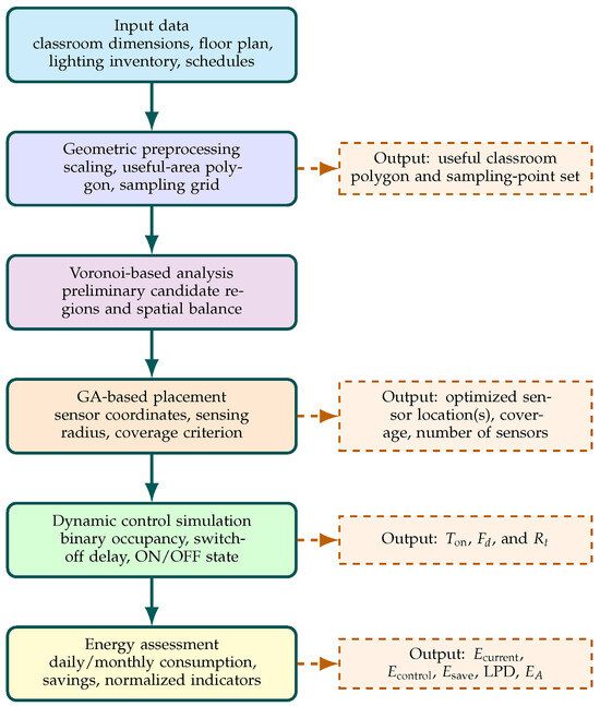
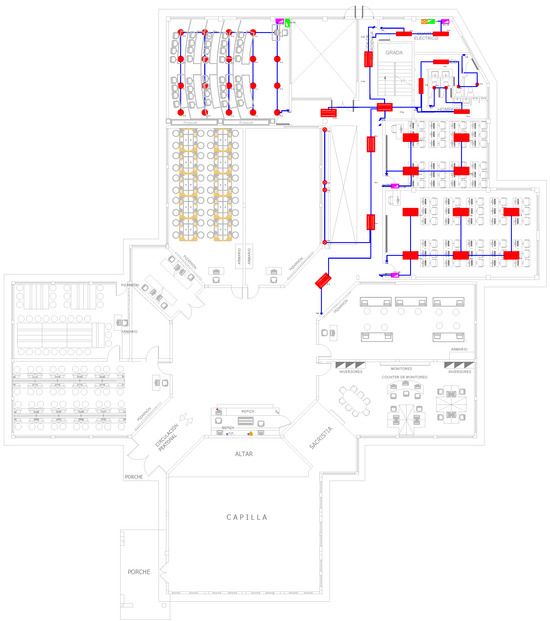
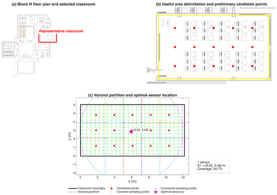
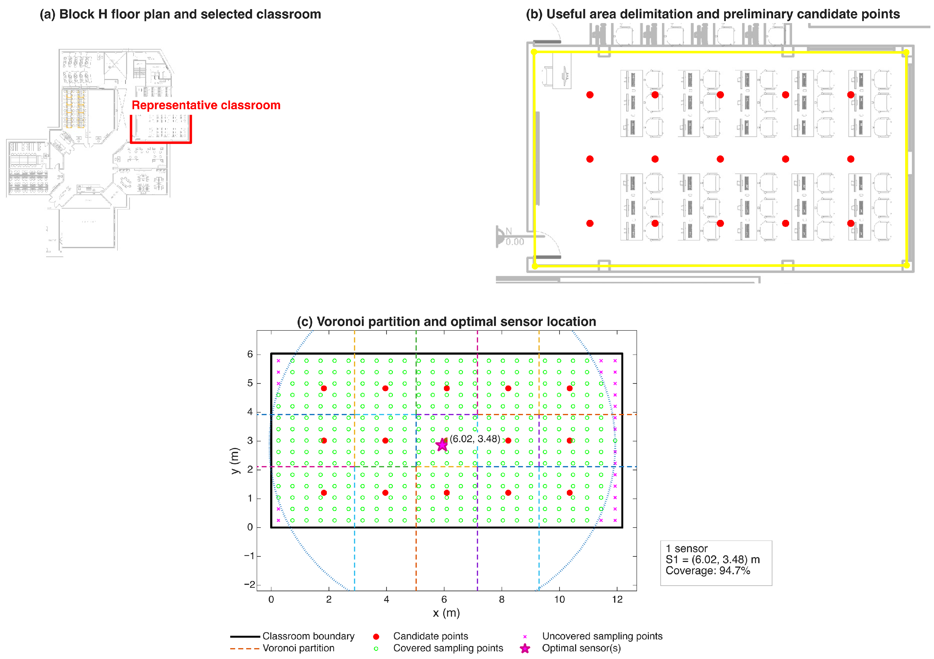
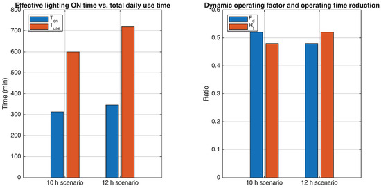
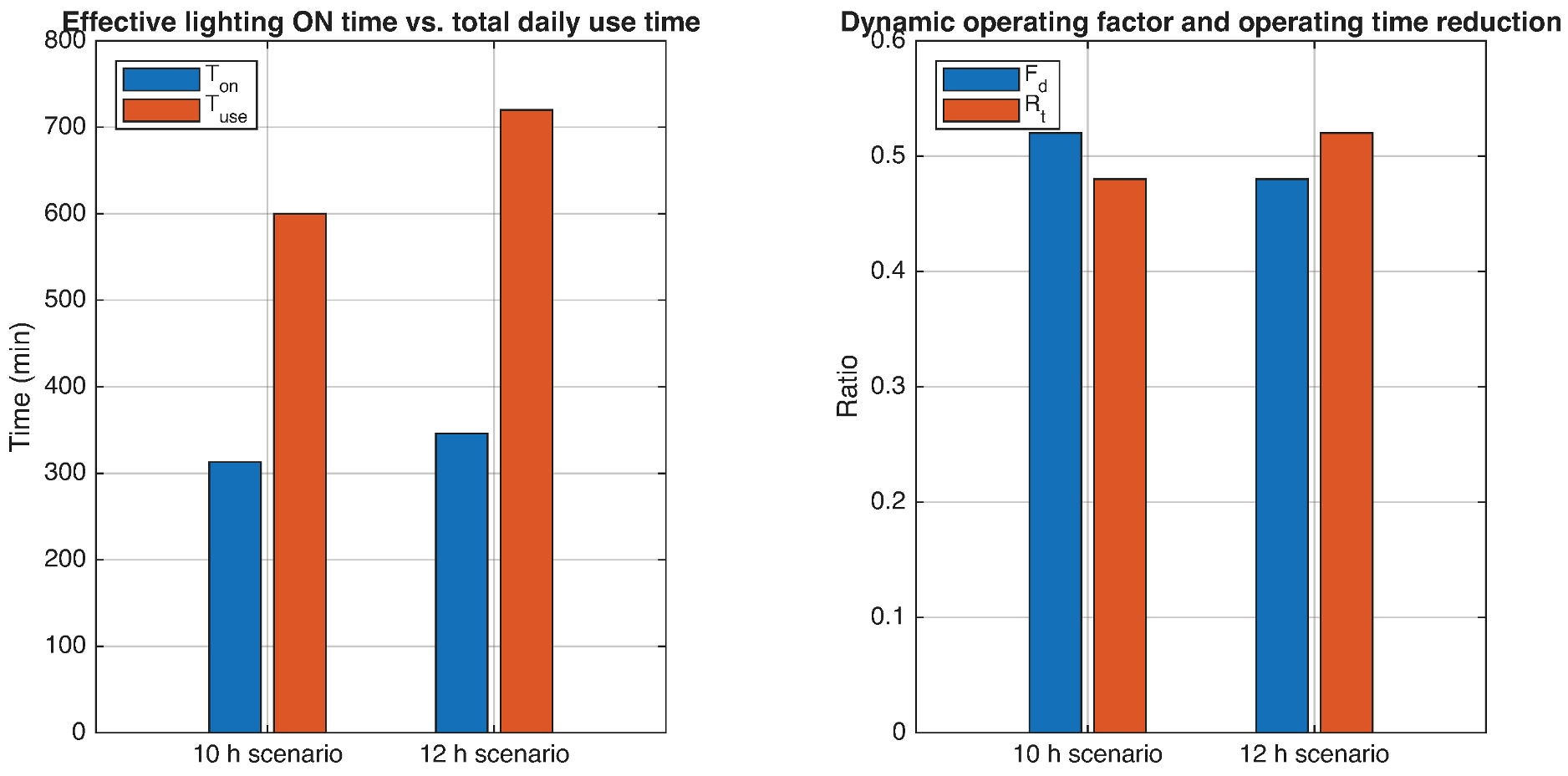
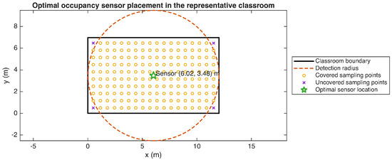
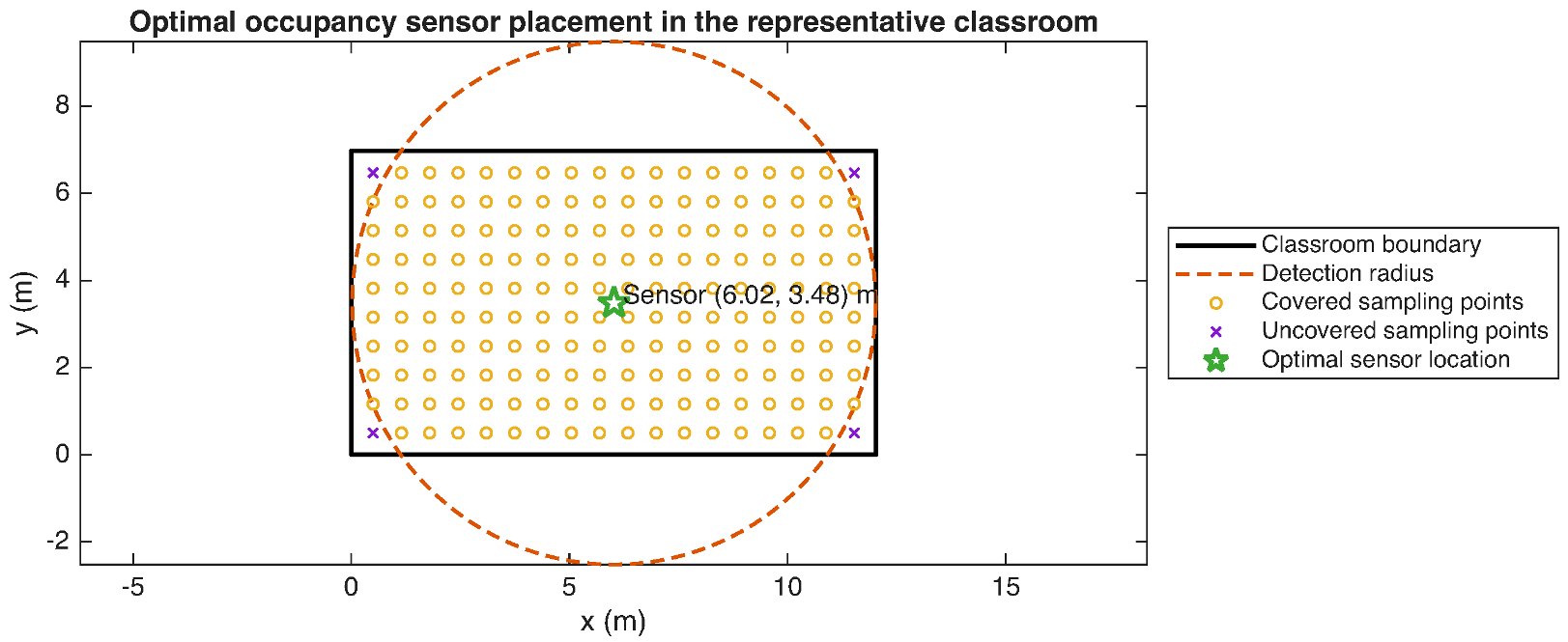
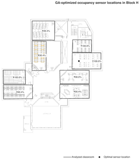
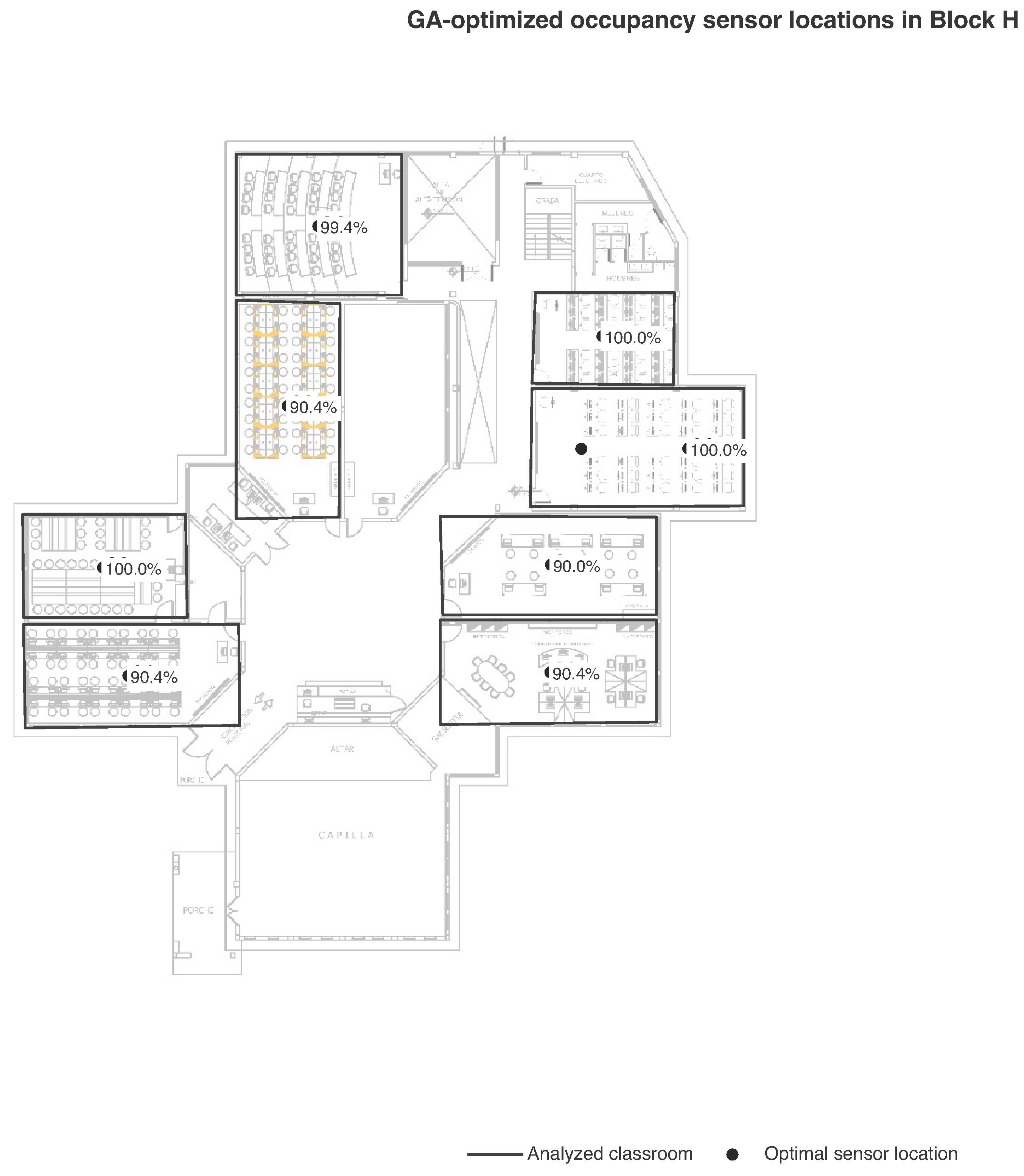
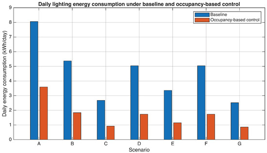
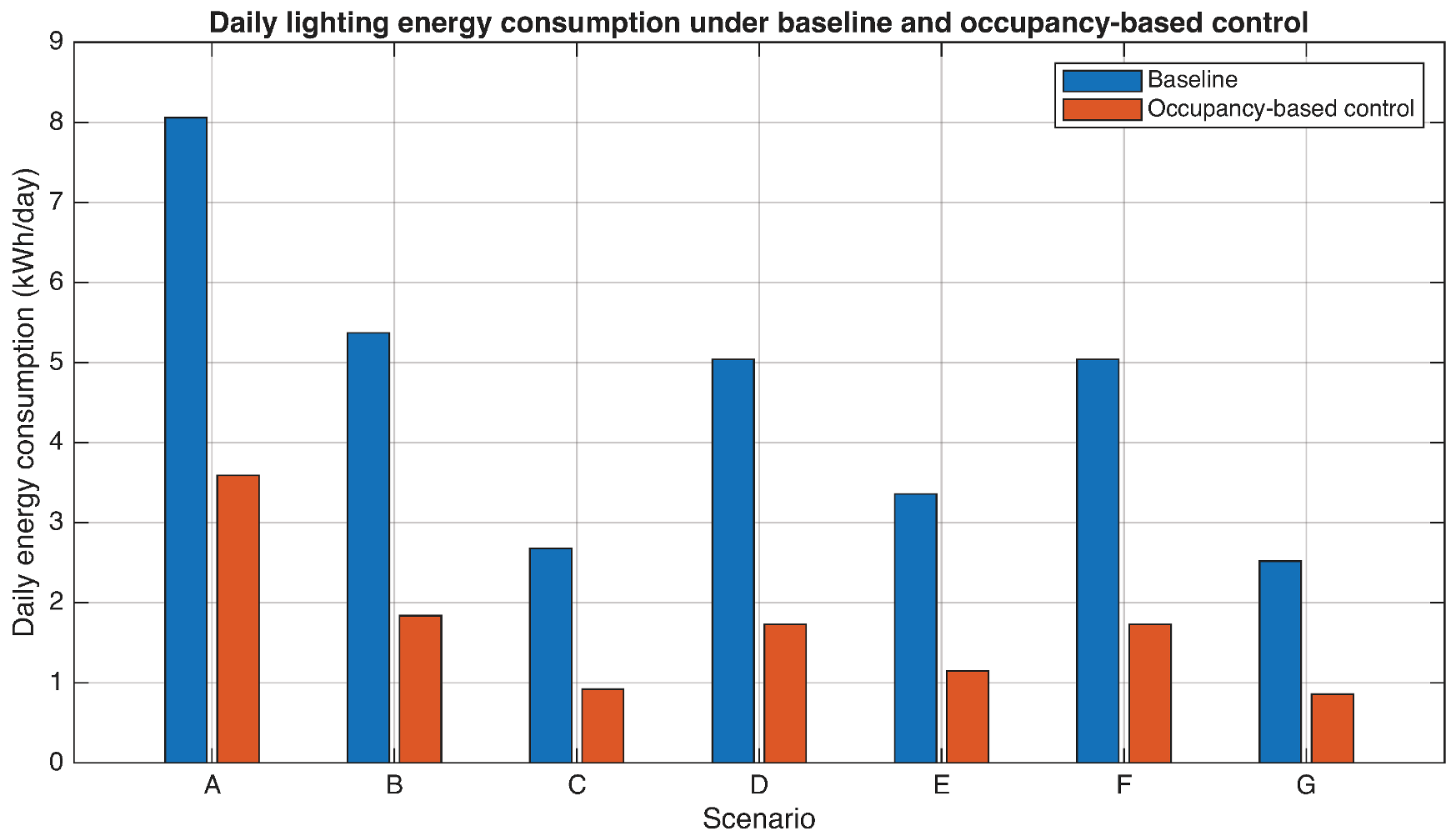
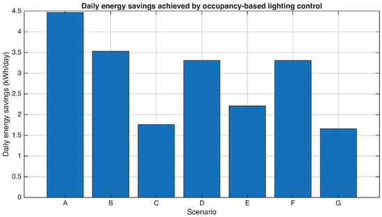
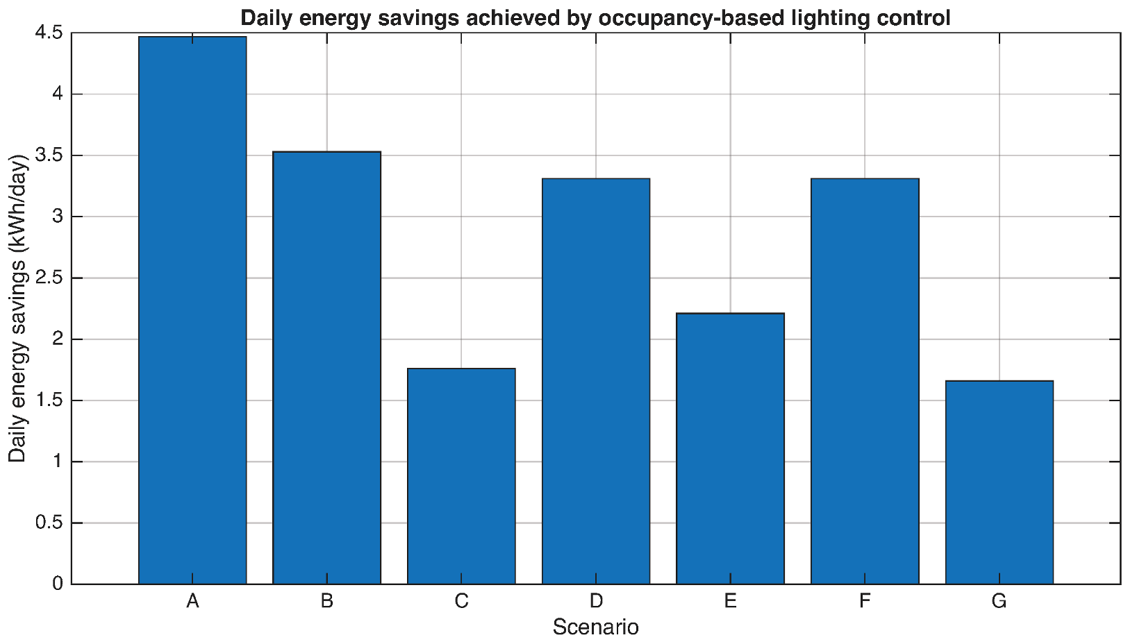
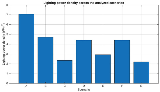
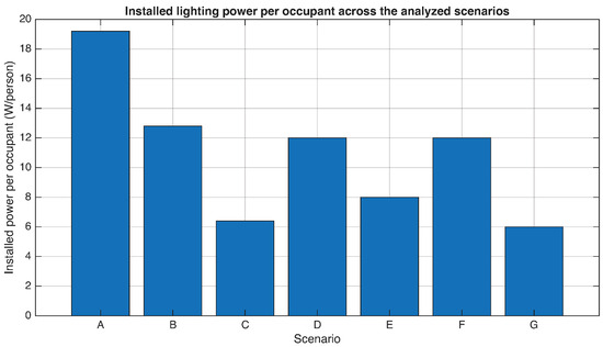
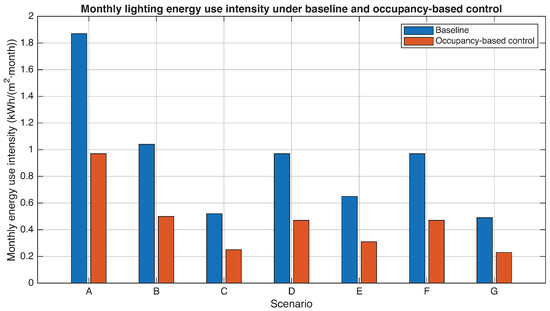
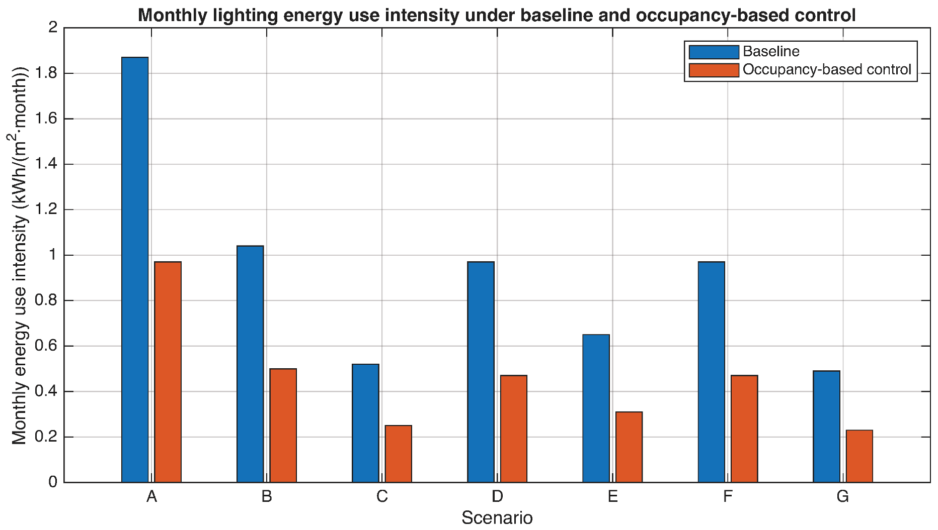

Disclaimer/Publisher’s Note: The statements, opinions and data contained in all publications are solely those of the individual author(s) and contributor(s) and not of MDPI and/or the editor(s). MDPI and/or the editor(s) disclaim responsibility for any injury to people or property resulting from any ideas, methods, instructions or products referred to in the content. |
© 2026 by the authors. Licensee MDPI, Basel, Switzerland. This article is an open access article distributed under the terms and conditions of the Creative Commons Attribution (CC BY) license.