A Dynamic Comparison of the Cost-Effectiveness of Carbon Pricing Policies

Abstract

To meet the goals of the Paris Agreement of avoiding dangerous climate change, decarbonisation of the global economy needs to proceed around three to five times faster over the coming decade than over the past two decades. This poses a great challenge for policy. Carbon pricing has often been put forward as the most efficient, or cost-effective, policy for achieving decarbonisation. This paper uses a stylised agent-based model to investigate whether implementing non-equilibrium dynamics and endogenous innovation results in more effective emission reductions for carbon tax compared with emission trading schemes. We find that the implementation of a carbon price is not policy-agnostic and that a carbon tax achieves faster emissions reduction, lower cumulative emissions, and lower cumulative (potentially wasted) investment in fossil fuel assets than a cap-and-trade policy with the same average carbon price. While a comparison between carbon pricing and alternative policies is outside the scope of this paper, we consider the broader policy implications that may be drawn from a new theoretical explanation for the difference in performance of the alternative carbon pricing approaches, and suggest that the traditional view that policy should aim to minimise the marginal emissions abatement cost is mistaken.

1. Introduction

In the context of a climate emergency, the need for a more urgent transition to low-carbon solutions within business is pressing [1]. Economists and economic institutions often propose carbon pricing to be the most efficient, or cost-effective, policy for achieving decarbonisation. Examples include the World Bank [2], the International Monetary Fund [3], and the Economists’ Statement on Carbon Dividends [4], signed by 27 Nobel Laureate economists, four former chairs of the US Federal Reserve, fifteen former chairs of the US Council of Economic Advisers, and two former secretaries of the US Department of the Treasury. Others have contested this proposition. A review of ex-post analyses of the effectiveness of existing, relatively high-price carbon pricing schemes found these had reduced emissions by incentivising greater efficiency in fossil fuel systems, but had had no effect at all on zero-carbon investment [5]. While this debate remains open, and while carbon pricing continues to feature prominently in economists’ advice to policy, governments have a strong interest in understanding what form of carbon pricing policy is likely to be most effective. Governments and the research community have a related interest in identifying the most appropriate analytical tools for comparing policy options.

The policy options under consideration for implementing a carbon price are defined for our purposes as follows:

• Cap-and-trade: A cap-and-trade system places a limit (the cap) on emissions within a defined area of economic activity. Firms that wish to emit carbon through their activities are required to buy permits to cover these emissions, and the supply of these permits is limited by the cap. Firms can trade permits, and the carbon price emerges from this market. The cap is usually, though not always, set to decrease over time.
• Tax: A tax requires firms within a defined area of economic activity to pay a fixed price for each tonne of carbon they emit. This price can be kept level or changed over time by governments.

Carbon pricing has generally been justified by either of two theoretical arguments [6]. For much of the last century [7], environmental pollution has been considered a negative externality. The policy prescription following from this analysis is that the negative externality should be priced to correct the market failure. For the last sixty years [8], an alternative interpretation has been to consider environmental pollution as a property rights problem. In this case, establishing a market to allocate the property rights is the recommended solution. The former argument provides the underlying rationale for a carbon tax; the latter argument provides the underlying rationale for a carbon cap-and-trade system.

Importantly, at a fundamental level, these two economic rationales are the same [6]. Both approaches result in a price being applied to the cause of pollution (in our case, carbon)—directly in the case of a tax; indirectly in the case of cap-and-trade. In both cases, theory predicts that firms will reduce their emissions up to the point where their marginal abatement costs are equal to the carbon price. In both cases, this is considered to lead to a cost-effective resolution of the environmental problem because it equates marginal abatement costs across all sources of pollution. This ‘optimal allocation’ of costs (or rights) allows the least-cost opportunities for decarbonisation to be accessed first.

According to this theory, which we will refer to as the ‘traditional view’, carbon taxes and cap-and-trade are expected to be ‘perfectly equivalent’ in regard to incentives for emission reduction and the overall costs of emissions reduction [6,9,10,11], The two approaches are also considered either equivalent or near-equivalent in regard to effects on competitiveness, possibilities for raising revenue, costs to regulated firms, and distributional impacts [6,11].

Theoretical debate has centred on the effect of uncertainty. Weizman [9] argued that if climate damages increase more steeply with emissions than abatement costs increase with emissions reduction, then cap-and-trade is preferable because the costs of a policy design ‘mistake’ (reflecting the regulator’s uncertainty) would be higher in the case of a tax; and vice versa. Nordhaus [10] extended this argument to propose that since climate damages depended on emissions stocks, which were relatively insensitive to near-term emissions reductions, while abatement costs were highly sensitive to near-term emissions reductions, a tax would be more efficient. Nordhaus [10] further argued that, compared to the fixed price of a tax, the potential volatility of the carbon price under cap-and-trade was a disadvantage as it could have disruptive effects on energy markets, investment planning, and other economic variables. Others have argued that a cap-and-trade system incorporating banking and borrowing of emissions permits can enable businesses to respond more efficiently to changing expectations than they could under a tax [12], leading a review of this literature to conclude: ‘These considerations suggest that the uncertainty dimension does not clearly favour any single emissions pricing approach’ [11].

The theoretical literature has recognised differences between the two policies in terms of practical considerations. Taxes have long been seen as likely to be advantageous in relation to complexity and administrative requirements [6,10,11], and more recently have been identified as superior in relation to interactions with complementary policies [11]. On the other hand, cap-and-trade has been argued to have the advantage of greater ease of linkage with policies in other jurisdictions [6].

Empirical studies are similarly inconclusive. One meta-analysis based on 81 studies published between 2011 and 2022 finds that the effect of carbon taxes on reducing emissions is stronger than that of cap-and-trade policies [13]. Another study using a panel sample of 100 countries reaches the opposite conclusion [14]. A further review of empirical studies finds that no strong conclusions about the relative performance of the two policies can be drawn, observing that performance depends on policy design and national circumstances, the emissions reductions achieved by either policy are almost always estimated in relation to a hypothetical ‘business-as-usual’ scenario which is itself uncertain, and these effects cannot be confidently separated from the emissions reductions achieved by other (non-carbon pricing) policies, which in most countries were probably larger [15].

Carbon pricing policies have also been studied with a wide variety of economic models. Integrated assessment models have generally focused on identifying an appropriate level of carbon pricing rather than identifying an effective policy design. Computable general equilibrium models have been used to compare carbon pricing policy design options and their distributional effects [16,17], while DSGE models have been used to consider how the performance of the two policies may be affected by economic shocks [18], with neither approach challenging the theoretical assumption of fundamental equivalence. Agent-based models have mainly been used to study one form of carbon pricing or the other [19]; we return to the exceptions to this below. Informed by the traditional view that the two policy approaches are fundamentally equivalent, the choice for public policy has been considered one of preference: would society prefer to have certainty over costs, but uncertainty over the rate of emissions reduction, or vice versa? Environmental interest groups have tended to show ‘a strong preference for cap-and-trade over taxes, in part because these interest groups prefer policies that help obscure the costs, but make benefits transparent and visible’ [6]. For similar reasons, politicians have favoured cap-and-trade systems with freely allocated allowances over either cap-and-trade with auctioned allowances or taxes [6].

Whether for these reasons or for others, emissions trading schemes (including cap-and-trade and other variants) are currently dominant, covering almost three times as many carbon emissions as carbon taxes [6]. Emissions trading schemes are either operational or under development in many of the world’s largest-emitting countries and regions, including the EU, China, the USA (at sub-national level), India, Brazil, Japan and Korea. Some policies are hybrids of the two approaches. Following concerns over the effectiveness of its Emissions Trading Scheme [20], the EU introduced a Market Stability Reserve, which makes the scheme behave somewhat less like a pure cap-and-trade system and more like a tax.

Have governments made the right choice? Or could a carbon tax reduce emissions more cost-effectively?

In this paper, we reconsider these policy options first from a theoretical perspective and then conduct a systems mapping analysis to better understand the different dynamics activated by each policy option. We then test in a stylised agent-based model (therefore embedding disequilibrium dynamics) whether accounting for dynamic relationships and endogenous innovation follows the results from the system mapping exploration, comparing the efficacy of the two different policies under equal conditions.

2. Reconsidering the Theoretical Assumptions

The traditional view that a carbon tax and a cap-and-trade policy are equivalent in the incentives they create for emission reduction and in the overall costs of emissions reduction (with their actual effects subject to the uncertainties and practical considerations discussed above) rests on three fundamental assumptions:

• Assumption of no path dependence: That for the economic system of interest, the options available at each point in time are independent of what has happened before.
• Assumption of equilibrium: That the economic system of interest can be considered to be in equilibrium over the time period of interest.
• Assumption of extrapolation: That the behaviour of the economic system of interest can be extrapolated from the behaviour of an individual agent within it.

We consider the validity of each of these assumptions in turn within the specific context of a transition to a low-carbon economy.

2.1. No Path Dependence

The traditional view predicts that a cap-and-trade policy and a carbon tax of equivalent stringency will have the same effect because, in either case, firms will reduce their emissions up to the point where their marginal abatement costs are equal to the carbon price. Either of these approaches will allow emissions reductions to be made wherever they can be made most cheaply, leading to the optimal allocation of economic resources.

The aim of carbon pricing, however, is to achieve change over time: to move from a high-carbon economy to a low-carbon economy, and to do so in a cost-effective manner. This is a challenge of dynamic efficiency [21].

In concluding that a policy designed to optimise allocative efficiency will necessarily lead to the most cost-effective change over time, the traditional view assumes that allocative efficiency and dynamic efficiency are the same. This can only be expected to be true if there is no path dependence in the economy. Without path dependence, the same set of options is available at each moment in time regardless of what has happened before, and therefore a policy that chooses the least cost option for emissions reduction at each moment in time will also achieve the least cost emissions reduction over the course of time. With path dependence, options for emissions reduction that are relatively high cost early in time may enable options that are much lower cost to be adopted later in time; consequently, there is no reason to expect that a policy that chooses the least cost option at each moment in time will also achieve least cost emissions reduction over the course of time.

Path dependence has long been recognised as a general characteristic of the economy [22]. In particular, it is characteristic of situations involving technological change, since new technologies tend to benefit from increasing returns to scale [22]. Such increasing returns to scale—with costs falling exponentially in proportion to cumulative deployment—are clearly observable for technologies central to the low-carbon transition, including solar photovoltaics, wind power, batteries, and hydrogen electrolysers [23].

2.2. Equilibrium

The traditional view that carbon pricing can achieve least-cost decarbonisation by optimising the allocation of economic resources is based on the premise that an optimal allocation of economic resources exists. The possibility of an optimal allocation of resources has been demonstrated by Pareto, but only under conditions of equilibrium.

A general definition of equilibrium in economics is ‘a situation in which nobody has any immediate reason to change their actions, so that the status quo can continue, at least temporarily’ [24]. This contrasts markedly with the challenge of decarbonising the global economy, which requires ‘rapid and far-reaching transitions in energy, land, urban and infrastructure (including transport and buildings), and industrial systems… systems transitions [that] are unprecedented in terms of scale…’ [25]. Systems transitions involve transformative change, in which many actors change their actions, and the status quo—the ‘socio-technical regime’ of technologies, infrastructures, institutions, production and consumption in the economic system concerned—is upended and replaced with a new regime [26]. Thus, in the context of a low-carbon transition, it appears entirely inappropriate to assume equilibrium. To confirm this view, we can consider three more specific definitions of equilibrium [24] and their applicability to problems of decarbonisation.

In microeconomics, equilibrium is defined as a balance between supply and demand: it exists where the supply and demand curves cross, resulting in an equilibrium price that clears the market. In a simulation, even in a simple market with one good, such an equilibrium is unlikely ever to be reached if agents’ trades are separated in time and space, rather than settled at once in an organised auction [27].

In macroeconomics, equilibrium refers to a situation when activities and price levels are such that the plans of various groups, such as savers and investors, are consistent, so that they can all be implemented, and nobody has any immediate need to change their plans. This situation cannot be expected to arise on any scale of time or economic activity that involves either fundamental uncertainty or technological change [28,29].

In game theory, equilibrium (a Nash equilibrium) exists when, given the strategies that all agents are using, no individual agent finds any change in strategy to be desirable. In a study of the generic properties of a set of randomly constructed different games [30], convergence toward equilibrium was found to be unlikely in any but the simplest and least competitive. In a set of relatively competitive games involving only two players, in which each could choose between ten possible moves, less than 3% of games tended to converge on an equilibrium.

A low-carbon transition, even within one sector in one country, fits none of these descriptions. It will involve many more than two actors in competitive situations with many more than ten possible moves. It will involve technological change, by definition, and will unfold over a timescale of years if not decades, implying considerable scope for fundamental uncertainty.

2.3. Extrapolation

The traditional view assumes that if the incentives facing an individual firm under different carbon pricing policies are the same (e.g., a firm is incentivised to reduce its emissions until its marginal abatement costs are equal to the carbon price), then the aggregate outcomes across the part of the economy covered by the policy will also be the same. This implies that the behaviour of the system of interest (a part of the economy) can be extrapolated from the behaviour of the individual agents within that system.

In complex systems in general, the behaviour of a system cannot be extrapolated from the behaviour of one of its individual components. Instead, complex systems display emergent behaviour that arises from the interactions of their components but is qualitatively different from that of their components individually [31]. This property of emergence is observable in economic phenomena such as bubbles and crashes [28] and processes of innovation [32]. Since low-carbon transitions involve many actors, interacting in complex ways over significant periods of time, an assumption of extrapolation (or ‘no emergence’) appears hard to justify.

2.4. An Alternative Theoretical Paradigm

If none of the assumptions of no-path dependence, equilibrium and extrapolation is valid in this situation, then the logic underpinning the traditional view entirely breaks down. We have no reason to expect the different carbon pricing policies to be equal in their effect. Comparison must instead be undertaken using methods free from those assumptions, so that the effects of path dependence, disequilibrium, and emergence can be taken into account.

Complexity economics offers a different theoretical paradigm within which these policy questions can be explored. It does not assume equilibrium, extrapolation, no-path dependence, or rational expectations; instead, it views the economy as a complex adaptive system whose behaviour emerges from the interactions of its components [28]. Within this paradigm of a disequilibrium economy, feedback (closed loops of cause-effect relationships) is seen as central to understanding processes of change. Consistent with this complexity (or evolutionary) economics paradigm are the qualitative studies of past socio-technical transitions [33] and the application of this understanding to the low carbon transition [34,35], and quantitative analysis of low carbon transition policies using disequilibrium models incorporating heterogeneous agents, uncertainty, and endogenous innovation [36,37].

Analytical tools consistent with this paradigm have been used in a limited way to compare the options of a carbon tax and a cap-and-trade policy. The physicist James Hansen used the principles of systems mapping to argue [38] that a cap-and-trade scheme and a tax-and-dividend policy would create different dynamics in the economic systems they aimed to influence: in a cap-and-trade scheme, any steps taken by one actor to reduce emissions would lessen the incentives for others to do likewise; whereas with a tax-and-dividend policy, steps taken by one actor to reduce emissions would increase the incentives for others to follow. For this reason (and others), Hansen argued that the two policy approaches were fundamentally distinct, and that tax-and-dividend was clearly preferable. Hansen did not explicitly consider the option of tax without a dividend, but it can be inferred from his logic that this would be expected to perform better than a cap-and-trade scheme and worse than a tax-and-dividend policy.

Chappin [39] compared a carbon tax with a cap-and-trade scheme using an agent-based model (ABM) of an electricity system, with the two policies set at equivalent levels of stringency (having the same average carbon price over the course of the simulation). The results showed a carbon tax significantly outperformed the cap-and-trade policy in three respects [39]: it achieved faster emissions reduction; it did so while producing a lower cost of electricity over the period in question; and at the same time, it led to a larger transition from incumbent to new technologies in terms of their relative market share. Foramitti, Savin, and van den Bergh [19] used an agent-based model to compare the two policy options, with the policies calibrated to achieve the same emissions reduction targets. In this study, the carbon tax outperformed the cap-and-trade policy by achieving the emissions reduction at a lower cost. Davis, Thurber and Wolak [40] ran a series of participatory games in which students acted as players in an electricity market, competing to maximise their profits. Across games where the two policies were matched in terms of emissions targets, mean emissions, and mean carbon prices, respectively, the cap-and-trade policy consistently led to much higher electricity prices without achieving lower carbon emissions. The analytical techniques used in these examples (systems mapping [41], agent-based models, and agent-based games) were unconstrained by assumptions of no path dependence, equilibrium, or extrapolation (no emergence) and may therefore be considered appropriate to the nature of the problem. However, these studies were limited in their consideration of innovation. In one [19], each firm has its own fixed menu of options for emissions reduction with its associated costs. In another [40], technology options are similarly static. In a third [39], innovation is represented as exogenous: technology costs change as a function of time. Innovation is increasingly recognised as one of the most important drivers of emissions reduction [42]. A systematic review of empirical literature on induced innovation in energy and related technologies [43] found strong evidence for technology costs declining as a function of cumulative investment and concluded that ‘endogenising innovation in large-scale models is important for deriving policy-relevant conclusions.’

In this paper, we first conduct a qualitative systems mapping exercise to compare the two policy options in the presence of technological innovation. We then present a new stylised ABM to compare the two policies, which includes the dynamics of innovation within the model. These are complementary methods. Both build on complexity economic theory [28], as described above. In the systems mapping, the dynamics of the system are understood by mapping the relationships between variables—based on logical reasoning (such as the relationship between supply, demand and price) or empirical evidence (such as the relationship between cumulative investment and technology cost reduction [23,26])—and identifying feedbacks. In the ABM, the dynamics of the system are discovered by simulating the interactions between agents, where each agent’s behaviour is driven by a set of decision-making rules that it is assumed to have. We apply these different methods independently, allowing the conclusions of each to be compared when they are applied to the same problem.

3. A Systems Mapping Approach to Policy Evaluation

To compare the dynamic effectiveness of the carbon pricing policy options, we conducted a systems mapping exercise [41]. The focus of this exercise was on identifying feedbacks in the economic system of interest—the power sector, its technologies, and the carbon pricing policies—that would either help or hinder rapid and cost-effective decarbonisation. Here, we consider the two basic policy options of a carbon tax and a cap-and-trade scheme. 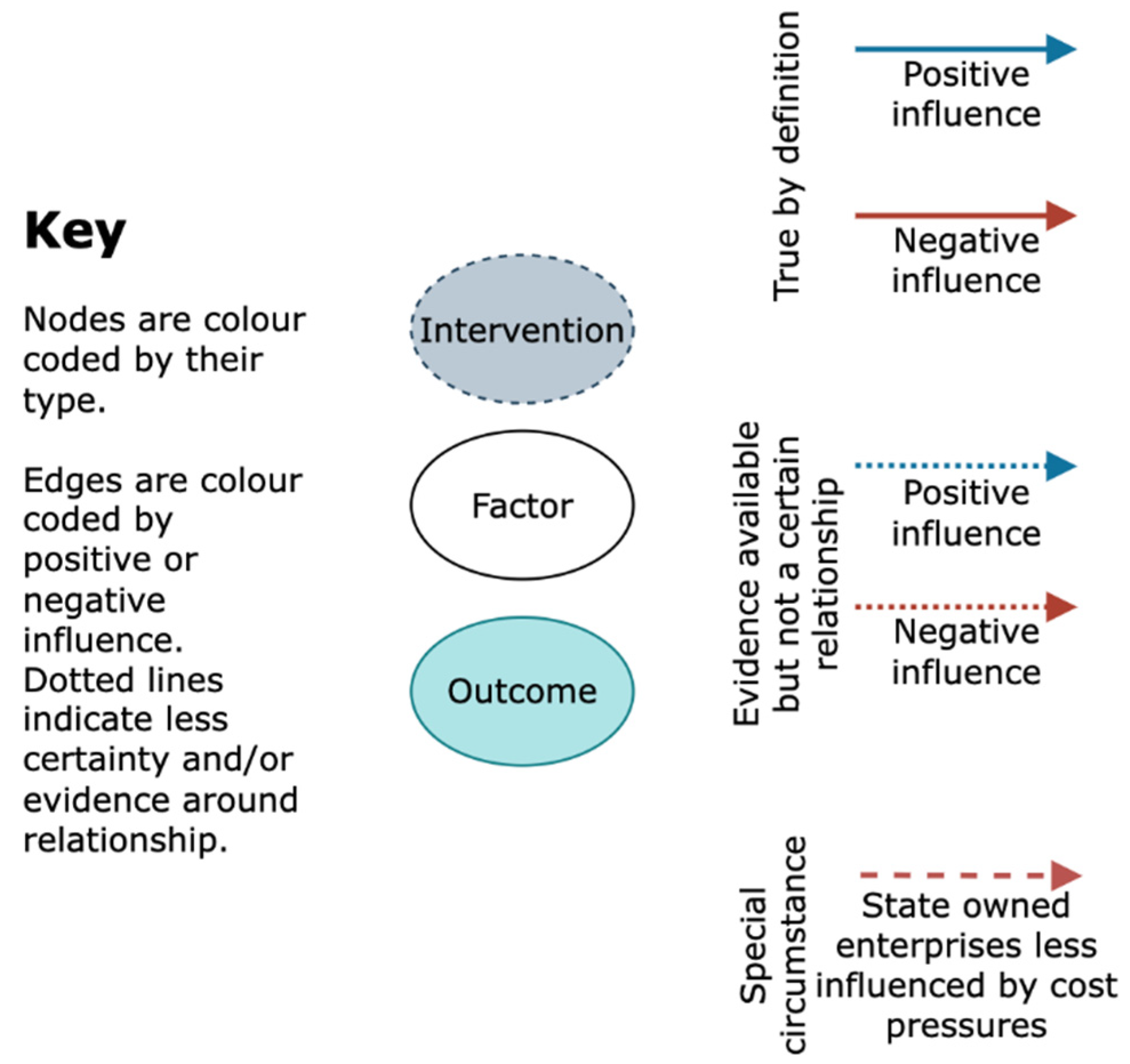In the Supplementary Material, we consider modifications to these policies and, finally, policy combinations. The key for these diagrams is shown in Figure 1.

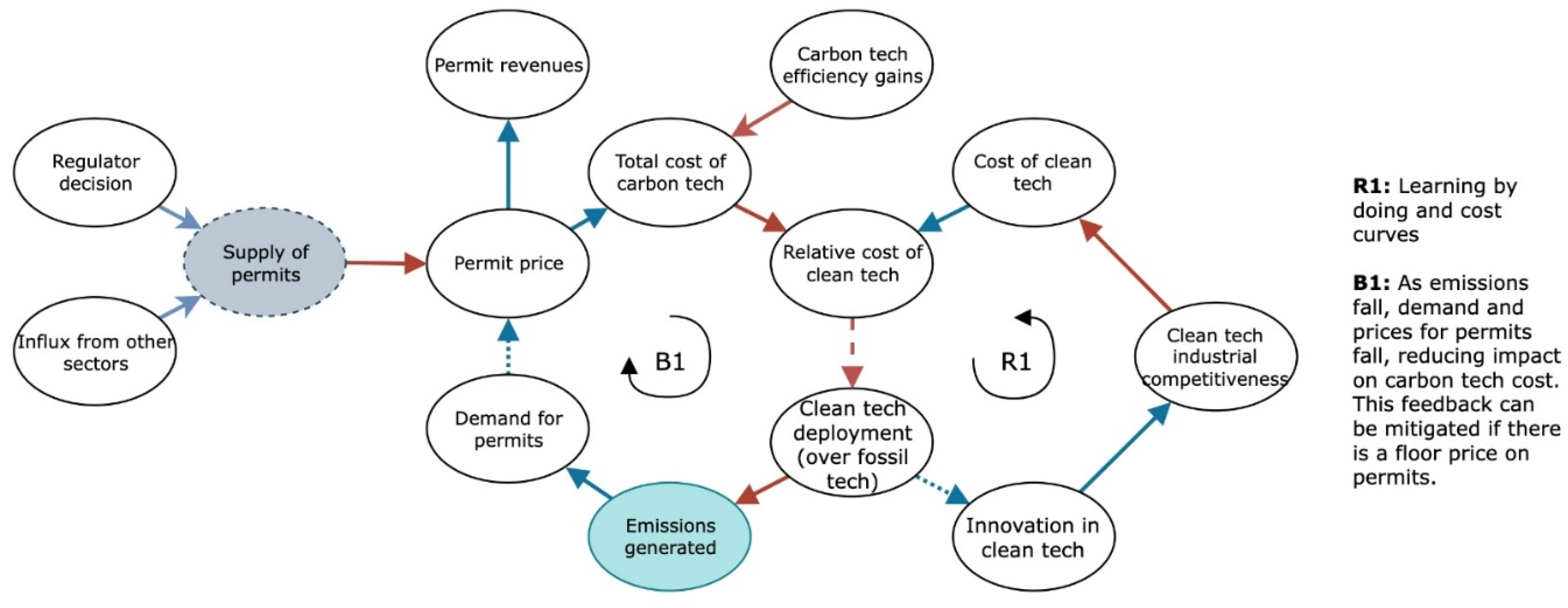
Figure 2 shows a system map of the power sector with a cap-and-trade policy in place. The right-hand side shows a feedback loop that exists independently of carbon pricing policy. As the cost of clean technology falls, so does its relative cost compared to fossil fuels; assuming there is some competition between technologies in the market, this causes a relative increase in its share of deployment. As clean technology deployment increases, so does innovation (broadly defined, including learning by doing and economies of scale); the industrial competitiveness of clean technology increases, and its costs come down. This reinforcing feedback is typical in the diffusion stage of new technologies and is consistent with the observation that the costs of wind and solar power are falling by constant fractions with each doubling of cumulative deployment, following Wright’s Law [44].

The left-hand side shows the effect of a cap-and-trade carbon pricing policy, in which emissions permits are traded, and their supply is fixed by a cap. The policy can be seen to create a balancing feedback, as follows. If the price of emissions permits increases, this increases the total cost of fossil fuel technology and therefore reduces the relative cost of clean technology. This causes an increase in the deployment of clean technology, leading to a fall in emissions. The fall in emissions reduces demand for emissions permits, whose supply is fixed by the cap, and whose price therefore falls.

The balancing feedback created by the cap-and-trade policy will give it a self-limiting effect. Any progress made by this policy will reduce its ability to incentivise further progress. Similarly, as the two feedback loops in this system interact, any stronger incentives for change that are created by progress in clean technology innovation and cost reduction will result in a lower carbon price, to some degree offsetting their effect. In the same way, the balancing feedback will also tend to offset any progress induced by other policies (such as clean technology subsidies, whether or not they are funded by carbon pricing revenues) or any changes in external conditions that lead to lower emissions—since these will reduce demand for permits, reduce the carbon price, and so reduce the incentive for further change. Instead of riding its luck and pushing ahead with the transition, the policy acts like a shock absorber, lessening the impact on the system of anything that might help move it forward. If the carbon price does act as a constraint on the system (i.e., it is not irrelevant), then under this policy, the trajectory set for the emissions cap can also be expected to act as an emissions floor.

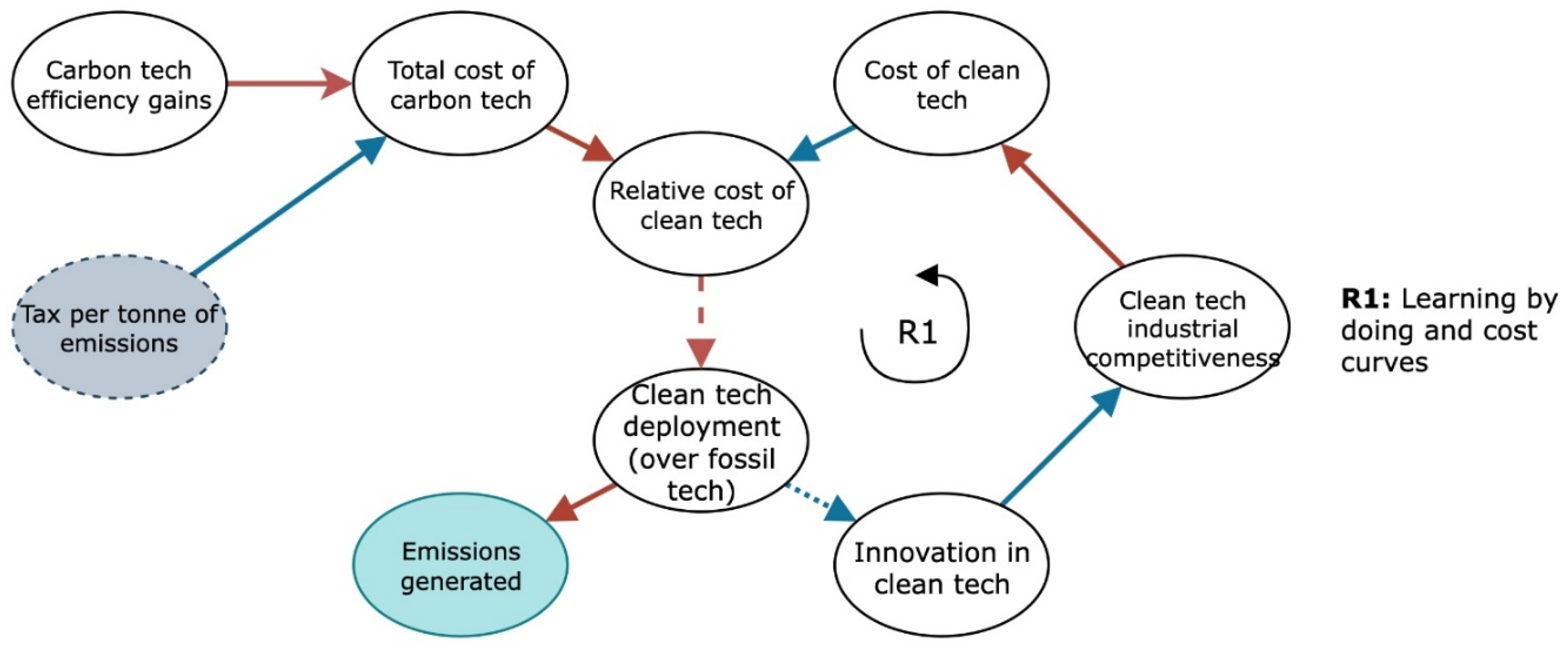
Figure 3 shows the system with a simple fixed carbon tax, where the revenue is kept by the government. The carbon tax increases the cost of fossil fuel technologies and so reduces the relative cost of clean technologies, strengthening the reinforcing feedback of clean technology diffusion.

The tax creates no additional feedback. Since there is no link between emissions reductions achieved and the level of the carbon price (as the tax is fixed), there is no balancing feedback as seen in the cap-and-trade system. This means the tax policy is not inherently self-limiting; neither will it offset the effect of the reinforcing feedback of clean technology diffusion. Equally, there will be no offsetting of the effects of any other policies (such as clean technology subsidies) or external influences. If economic growth is lower than expected, the incentive for decarbonisation provided by the tax will not be any less. If revenues from the tax are recycled into clean technology subsidies, further reducing the relative cost of clean technologies compared to fossil fuels, this will further strengthen the reinforcing feedback of clean technology diffusion.

This comparison reveals a fundamental difference in the dynamics created by the two policy options. It suggests that all else being equal, in a competitive market, a carbon tax is likely to be more effective than a cap-and-trade scheme of equivalent strength. It is, of course, possible to modify the policy designs to produce policies that are neither pure cap-and-trade nor tax systems, and many variations are possible (see Supplementary Material).

The policy implications of these findings must be described with caveats, which we address in the discussion section below. However, the findings of the system mapping exercise appear significant: the dynamics of the tax policy are superior to those of the cap-and-trade policy, and this difference is magnified both by the addition of revenue recycling and by the combination with other policies.

4. Methods

In this paper, we present a new stylised agent-based model, aimed at further exploring the dynamics outlined in the systems maps from the previous section, while addressing some of the key limitations identified in previous attempts at modelling alternative carbon pricing approaches (in particular the assumption of equilibrium economics) as well as embedding innovation within the model, instead of treating it as exogenous. We consider an ABM appropriate for the purpose of comparing carbon pricing policy options because, unlike an equilibrium or optimisation model, an ABM does not assume a certain system behaviour in advance. Instead, by simulating the behaviour of economic agents, it allows the system behaviour to be discovered as an emergent property of the model. This makes ABMs well suited to analysing the actual and possible behaviour of complex systems, such as an economic sector undergoing technological change [41]. It is important to note that the aim of this ABM is not to recreate all the dynamics of a real electricity market or to make quantitative predictions, but rather to test the effects of endogenising innovation on the comparison between cap-and-trade and carbon tax as alternative decarbonization policies in a stylised environment.

The ABM that we present in this paper is developed with the Netlogo 6.3.0 software [45] and is freely available online on the COMSES repository [46].

The ABM recreates an abstract, competitive, closed electricity market which can be imagined as representing a stylised version of a national market with no interconnectors (i.e., no trade) to the global market. The agents in the model are the electricity generation companies that make decisions on which generation technologies to deploy, when, and how much. They can choose between four technologies: coal, gas, wind, and solar PV. Each company starts with a different mix of these technologies and has different expectations about the future. As the companies aim to maximise their profits [47], their decisions are a function of their expected returns, capital constraints, and other considerations described further below.

Demand for electricity is represented by an exogenous trend line and is assumed to increase by 5% yearly. The market works by a ‘merit order’ approach: the cheapest units of generating capacity are used first, and then increasingly expensive units are used until demand is met. The cost of the marginal unit of supply sets the electricity price, which is then paid to all suppliers. (Any surplus generating capacity is unused). The cost of each unit of supply is a levelized cost of electricity that includes capital costs (depreciation), operating costs (fuel and maintenance), and any carbon pricing costs.

The model runs three policy scenarios: (1) No Policy, where no policy is implemented to accelerate the transition to low carbon technologies, and companies continue to produce and invest along a ‘business as usual’ trajectory; (2) the Emission Trading System (ETS) scenario, where a cap-and-trade scheme roughly based on the EU ETS is introduced (described in more detail below), and, finally (3) the Tax scenario where a carbon tax is applied to all emissions at a fixed rate.

To test the impacts of the endogenisation of innovation on the effectiveness of the two alternative policies, the model can be run with either of two settings governing innovation—endogenous and exogenous. The ‘endogenous’ setting can be thought of as representing the total global market, within whose boundaries all clean technology innovation takes place—that is, all innovation is driven by the investment decisions of the agents within the model, who are influenced by policy (carbon pricing), by each other, and by their environment (a competitive market). With this setting, the cost of clean technologies reduces as a function of their cumulative deployment, following a Wright’s Law relationship based on historical data. In the ‘exogenous’ setting, the cost of clean technologies reduces as a function of time, following a Moore’s Law relationship based on the cost reductions resulting from the endogenous runs of the ETS model so that the outputs can be directly compared. This can be thought of as representing a market that is too small to significantly influence clean technology costs. That is, clean technology cost reduction is driven by external factors such as large-scale manufacturing in another region (a simplification, since in reality factors such as installation and finance costs are likely to be influenced by local policy even if the core technology costs are not).

Due to the stylised nature of the model and the theory-testing aim, the model is only partially empirically grounded, meaning that some of the data fed into the model, as well as the parameters used, have been gathered from available literature. In particular, the parameters defining the costs of different electricity generating technologies, and the rate at which these technology costs fall in response to deployment in the model, have been taken from a previous empirical study [48], and the rate of decrease for the emissions cap used to simulate the ETS scenario has been taken from the real functioning of the EU ETS [49]. The rest of the model and the parameters used have been based on a series of assumptions as discussed in the following sections. We acknowledge that this is an important limitation of the model, which should therefore not be used for prediction or policy development. However, as mentioned before, the aim of the model is simply to illustrate the effect of embedding the dynamics outlined in systems maps presented in the second section in a dynamic environment and test the impact on the efficacy of alternative carbon pricing policies [50]. Despite the limited scope of this paper and model, we see this as an important step towards understanding the real dynamics involved in a carbon tax and a cap-and-trade scheme.

4.1. Build Time, Lifetime, and Decommissioning of Technologies

Electricity-generating capacity is installed and managed in the model in ‘batches’. A batch is created when a company invests in new capacity for a particular technology. The size of the batch is variable: a company can invest in as many units of generating capacity as its capital allows. Capacity and investment costs related to each batch installed are stored in lists that track for each company and for each technology the capacities added, and the capital expended in each year.

Each batch of new generating capacity will come online after its build time has passed. Each batch of capacity installed is assigned a lifetime based on Mercure [48] (see initialisation of the model for the values assigned to these parameters), after which it will be decommissioned (The capacity installed in a specific year is ‘deleted’ from the capacity available for the company that owns it when it comes to the end of its lifetime).

4.2. Unit Costs of Electricity Generation and Profit Calculation for Companies

The cost of electricity generation is specific to each batch of (technology-specific) generating capacity owned by each company. It includes:

• Fuel costs (different for coal and gas, zero for solar and wind, no variance over time)
• Investment costs (different for each technology, varying over time), accounted for by linear depreciation over the lifetime of the asset
• Emission costs (either tax or permit costs)

The investment costs for each technology are taken from an empirically observed cost curve [48], where the cost of deployment of one unit of any particular technology in a given year is based on the cumulative capacity of that technology installed to date. This is the same for all companies, equivalent to assuming that all companies can buy the same technology from the global market. The cost curve formula is:

$${Iunitcost}_{t,i}=I_0{({\displaystyle \frac{{{\displaystyle {\sum }_0^t}w+W}_t}{W_0}})}^{-\beta }$$

(1)

where I₀ is the unit cost at the start of the simulation, β represents the learning factor for the particular technology, and w represents the capacity installed.

At any time, each company has a varied stock of electricity generation assets, all of which are incurring costs, and some of which are earning revenue. The profit of a company in a given year (adapted from [51]) is given by:

$${\pi }_{j,t}={Revenue}_{j,t}-{Icost}_{j,t}-{Fcost}_{j,t}-{Permits}_{j,t}-{Sanction}_{j,t}-{Tax}_{j,t}$$

(2)

J is the company, t is the time period (which we refer to as the ‘year’). Icost is the investment costs associated with the depreciation of capital assets, Fcost are the fuel costs related to operating fossil fuel technologies, Permits are the cost of permits bought in the ETS scenario, Sanction is the penalty paid for any emissions not covered by permits in the ETS scenario, and Tax is the cost of tax paid in the tax scenario (the tax rate times the CO₂ emissions of the company in that year). Revenue is calculated as the electricity market price multiplied by the sum of the amounts of generation provided by each technology for company j in year t.

To test the effect of different bidding strategies in the electricity market, we allow companies to calculate costs of units of power offered to the market in two ways; firstly by technology type for that company (I cost techno) and secondly as an average across all technologies owned by the company (I cost company)—although in this second strategy actual operating costs will still be different across technology types. This can be understood as representing two different behaviours of companies in the way they try to recoup their investments—one where they attempt to recoup by technology type (i.e., a company will manage its portfolio of solar technologies separately from its portfolio of coal power stations), and one where they attempt to recoup all investments into energy infrastructure regardless of technology type (i.e., where returns from a solar investment can pay for the investment costs of a coal power station). Since this is an important assumption, we adopt a parameter in the user interface of the model that defines the proportion of the final investment cost calculated with either calculation (avg-unit-cost-techvstot). This allows us to model different types of companies where technologies are blended across investments or where they are separated into different legal entities. This choice impacts how the depreciation cost of each unit of power generation that bids into the market is calculated, and therefore the overall merit order by which units of generation are selected. A market where companies wish to make a return on all of their sunk investment costs will see individual companies with the highest average sunk investment cost allowing their higher cost assets to become stranded (resulting in a higher concentration of stranded assets to companies more exposed to those technologies), while a market where companies wish to make a return on specific technology investments may see technology assets becoming stranded across a wider range of companies. In the model runs, we use a blend of the two options where individual companies try to mainly recoup the costs per technology but balance this slightly with a cross-company approach (parameter is set at 0.8).

When calculated by technology, the average unit cost for each technology, for each company, is the weighted average of the past unit costs divided by the capacity that the investment has generated, divided by the lifetime of the technology to account for depreciation. These costs include all sunk costs in investments already made, such that companies strive to keep solvent with their future investments. This is formalised mathematically as:

$${Iunitcostbytechnology}_{t,i}={\displaystyle \frac{{\displaystyle {\sum }_0^t}{I}_{i,j}}{{{\sum }_0^{t}C}_{i,j}}}/{Life}_i$$

(3)

where the sum of investments I for technology i made by company j is divided by the sum of capacity C invested in technology i by company j, divided by the lifetime Life of technology i.

When calculated by the company, the average unit cost per year for all technologies owned by the company is the weighted average of the past unit costs divided by the capacity for all the technologies owned by that company, divided by the lifetime of the technologies owned to account for depreciation. This is formalised mathematically as:

$${Iunitcostbycompany}_{t,j}={\displaystyle {\sum }_{i=0}^n}{\displaystyle \frac{{\displaystyle {\sum }_0^t}{I}_j}{{Life}_i}}/{{\sum }_0^{t}C}_j$$

(4)

where the sum of investments I for all technologies owned by company j is divided by the lifetime Life of the technologies, divided by the sum of capacity C invested in the technologies owned by company j.

The final investment cost is defined by the following equation:

$$\begin{array}{c}{Ifinalunitcost}_{t,i,j}={Iunitcostbytechno}_{t,i}\times par+{Iunitcostbycompany}_{t,i}\times \\ \left(1-par\right)+{Fcost}_{i,t}+{Permits}_{j,t}+{Sanction}_{j,t}+{Tax}_{j,t}\end{array}$$

(5)

where the investment unit cost by technology for technology i and company j is multiplied by the parameter par [0, 1] as defined in the user interface that defines which proportion of the final cost is calculated with each equation. This is summed to the Investment unit cost by company for company j, multiplied by 1 minus the parameter par, and summed to the fuel costs Fcost for technology i, summed to the Permits paid by company j, summed to the Sanctions paid by company j and summed to the Tax paid by company j. The Investment final unit cost is calculated for each technology owned by each company.

4.3. Agents’ Behaviours

As noted above, companies decide which electricity-generating technologies to invest in and decide the timing and scale of these investments, with the aim of maximising their profits. Companies differ in their competitive strategies (some are more aggressively expansionist than others) and in their expectations of the future profitability of different technologies, which are governed by their perception of future markets as below.

Companies know that if they make the right technology choices, their market share will increase, but they cannot predict by how much it will increase (if at all). We assume that all companies aim to increase their market share by at least 10%, and this guides their decisions on how much new generating capacity to acquire. However, the companies are not all the same. We define two behaviours related to market leadership (aggressivevsneutral parameter in

Table 1. Variables included in the model user interface and related initialisation values.

Variable	Definition	Value Range	Value Initialised
mean-start-capacity-coal	Coal start capacity for companies	[0, 100] MW	50 +/− [0, 20]
mean-start-capacity-gas	Gas start capacity for companies	[0, 100] MW	40 +/− [0, 20]
mean-start-capacity-wind	Wind start capacity for companies	[0, 100] MW	30 +/− [0, 20]
mean-start-capacity-solar	Solar start capacity for companies	[0, 100] MW	20 +/− [0, 20]
energy-demand-increase	Annual increase in electricity demand	[0, 1]	0.05
coal-economies-scale	Learning factor for coal used (I unit cost)	[0, 1]	0.044 (SA)
gas-economies-scale	Learning factor for gas used (I unit cost)	[0, 1]	0.059 (SA)
wind-economies-scale	Learning factor for wind used (I unit cost)	[0, 1]	0.105 (SA)
solar-economies-scale	Learning factor for solar used (I unit cost)	[0, 1]	0.269 (SA)
start-capital	Companies’ start-up capital	[0, 300,000,000,000] £	10,000,000,000
Aggressivevsneutral	Parameter that defines companies’ behaviours related to market leadership	[0, 1]	[0.8, 1.0] (SA)
ambitiousvnot-ambitious	Parameter that defines the likelihood of companies believing in the ETS’s effectiveness	[0, 1]	[0.8]
fossilvsrenewables-preference	Parameter that defines the likelihood of companies having a preference for fossil fuels or renewables	[0, 1]	[0.8]
avg-unit-cost-techvstot	Parameter that defines which portion of the final unit cost is calculated with either the weighted average by company and technology, or the average of all technologies	[0, 1]	[0.8]
investment-technology-threshold	Parameter that defines the minimum percentage needed for a company to invest in a technology	[0, 1]	0.1
start-tax	Variable that defines the start level of carbon tax	[0, 100] £	34
tax-increase	Variable that defines the 4-year increase of carbon tax	[0, 100] £	0
start-ets-cap	Variable that defines the start cap for the ETS	[0, 10,000,000]	4,000,000
ets-cap-reduction	Variable that defines the annual cap reduction for the ETS	[0, 100]%	2.2 (SA)
ets-sanction	Variable that defines a sanction when companies emit more than the permits they own	[0, 100] £	100

), which guide the amount of capacity the companies want to build every year:

• Aggressive—These companies will invest in increasing their generating capacity with the aim of increasing their market share by more than 10%
• Neutral—These companies will only invest to increase their market share by 10%

Parameters relating to company behaviours are defined in the user interface (see Table 1) and can be assigned values in the range 0 to 1. The value assigned to each of these parameters will correspond to a certain proportion of companies being assigned a specific behaviour. For example, if the parameter aggressivevsneutral is assigned a value of 0.3, 30% of the companies will be assigned a market behaviour of ‘Aggressive’ and 70% ‘Neutral’, with these characteristics randomly distributed among the set of companies. The parameters and related behaviours are listed below.

Companies have two behaviours related to their preference for the energy mix. This is a weighting factor that influences the company’s preference between fossil fuels and renewables (fossilvsrenewables-preference parameter in Table 1), representing their perception of the preferences of their customers and/or shareholders:

• Preference for fossil fuels
• Preference for renewables

This parameter relating to energy mix preference is also defined in the user interface (see Table 1) and can be assigned values in the range 0 to 1. We initially set this value at 0.8 to represent a more risk-averse market with a slight preference for incumbent technologies (fossil fuels). This weighting factor interacts with companies’ specific expectations of the profitability of different technologies when they make their investment decisions. This weighting factor shifts the mid-point of the randomised distribution of preference across companies so that a higher value sees a higher proportion of companies seeking to invest in incumbent technologies.

The companies have a behaviour related to different expectations of future prices of emissions permits in the ETS scenario (ambitiousvnot-ambitious parameter in Table 1):

• ETS low: permit price = previous year’s permit price − 3% (± 3%)
• ETS high: permit price = previous year’s permit price +10% (±5%)

The ETS price is uncertain because it emerges from the market. We have adopted an asymmetric future expectation as companies may expect the ETS price to increase as the emissions cap reduces, although this is not a given. If the technology mix shifts to renewables, the price can fall. Sensitivity analysis was used to test the impact of this asymmetry. In the Tax scenario, the carbon price is fixed and therefore certain. In both policy scenarios, we assume there is no change to the policy (the stringency of the cap or the level of the tax) over the course of the simulation.

Some randomness is introduced in the calculations of key parameters that define the behaviours to ensure some variability in the simulations. This can be considered to represent the wide variety of agents’ expectations that are likely in a context of uncertainty.

4.4. Expected Profit Calculation for Technologies, and Decision of Which Technologies to Invest in

Agents calculate the expected profit for each technology as follows:

$${expP}_{i,j}=({expPr}_i-{expIC}_{i,j}\times {\displaystyle \frac{1}{{life}_j}}-{FC}_i-{expPC}_j-{expTax}_j)\times {TP}_{i,j}$$

(6)

where the expected profit of company i from technology j, expP_ij, is calculated by the expected revenue from electricity generation for company i, expPr_i, minus capital depreciation (expected investment cost at the time of building expIC_i,j, which is not known for certain because the investment decision is made at the end of the year and the exact position on the cost curve depends on the total investment across all companies, divided by the lifetime of technology j), minus the fuel costs FC, minus the expected permit cost, expPC, minus the expected tax. The expected revenue is based on the market price of electricity, modified by a future expectation per company of higher or lower electricity prices. Expected revenue is not technology dependent because the company assumes that any unit of generating capacity that it acquires will be fully utilised. (This assumption is likely to create a bias in investment decision-making toward technologies that are higher up the merit order, which will not, in fact, always be fully utilised.) Capital depreciation is the total expected investment expIC that company i makes into technology j divided by the asset’s lifetime. The fuel costs are assumed to be constant over time. Finally, everything is multiplied by company i’s technology preference weighting factor for technology j, TPij. A weighting factor of zero means that company i has no desire to invest in technology j (for example, company i may be a renewable company not wishing to invest in coal, or a gas company not seeking to diversify). A weighting factor of one means that company i takes into consideration the full expected profit when making an investment decision. This factor allows us to create markets that are more or less likely to invest in renewables or fossil fuel assets. This weighting factor is generated through a randomised spread away from the mid-point weighting factor set previously (a higher weighting factor results in more companies preferentially investing in fossil fuels).

The amount of new capacity of each technology that a company invests in is proportional to the relative expected profits from each technology, and is calculated with the following formula:

$${CI}_{i,j}={\displaystyle \frac{{expP}_{i,j}}{{\displaystyle {\sum }_{j=0}^n}{expP}_i}}\times Q_i$$

(7)

Capacity invested CI is calculated for each technology j by weighting the expected profit expP of technology j by the sum of profits for all technologies for company i, and multiplied by the total amount of capacity that company i wants to build Qi. Any technology whose proportion of total expected company profits is less than 10% (or the % set in the parameter ‘investment-technology-threshold’ listed in Table 1) will not be invested in. This is to ensure there is a minimum size of investment made into any technology within any given cycle (this introduces the idea that a company would need a minimum size of project to justify an investment). For technologies with profits below 10%, the investments will be reallocated between the remaining technologies with shares of expected profits above 10%. This will be coupled with a check on the company’s available capital (see below). In this way, technologies with higher expected profit will be invested in preferentially.

Investment-related procedures start to take place from tick 1 (i.e., year 2) in the model. This is to allow for the model to initialise key variables needed in the calculations above, such as prices, unit costs and related behaviours.

4.5. Companies’ Capital and Default

The finances of energy companies are highly simplified in the model. Companies begin with an initial stock of capital. This is defined in the user interface (see Table 1), but for our simulations, we set the initial capital assigned to each company at £10 billion. Each company’s capital increases or decreases with the profit or loss that it makes each year. If companies run out of capital, they cannot acquire new generating capacity, but can continue to operate the assets they have with the aim of making a profit and investing again in future.

After calculating the amount of new capacity that each company wants to invest in, a procedure checks against their available capital. The desired amount of capacity for each technology is added to a series of company-owned lists along with the provisional investment costs associated with each batch. The lists are sorted in batches by capacity in order of their expected profitability. Every company then runs a loop to sequentially ‘invest’ in each batch included in its list, until either the investment wants are fully satisfied or it runs out of capital. In the case of the latter, the company will only invest and build as much technology as it can afford. Companies then update their lists with the new investments, which will come online after the build time has passed.

4.6. Electricity Price Determination and Companies’ Revenues

As mentioned above, the market price of electricity is set equal to the cost of the marginal unit of supply (the final and most expensive unit of electricity supplied to the market to meet demand). Companies do not apply a mark-up to the cost of electricity; their profits arise from the difference between the market price of electricity paid to all units of generation and the varying costs of those units of generation. The market price is expressed in £/MWh unit of electricity used. The company-owned lists containing the capacity available for each technology, for each company, along with the unit cost associated with each, are sorted based on the unit cost from smallest to largest. A loop procedure cumulatively adds the capacities from least to most costly until the ‘supply’ meets the overall demand calculated for that year. The unit cost of the last capacity needed to meet the demand will be the global electricity price. This is then used by the companies to calculate revenues. Each company ‘knows’ the amount of electricity it was able to sell at that price through the loop procedure mentioned above. The ETS scenario is activated when chosen via the dropdown list of scenarios in the model interface. In this scenario, companies try to buy enough emission permits to avoid incurring a sanction. Each permit corresponds to a tonne of CO₂. Each year, the falling emissions cap results in a decreasing amount of permits being available for companies to buy. All emissions not covered by permits incur a fine of £100 per tonne of CO_2. This scenario begins to affect companies from tick 1 (i.e., year 2). This is because the model requires the first year for initialisation. At the beginning of the second year, the ETS cap is set, and from the following year, it is reduced on a linear trajectory whose gradient can be set via the user interface. Data on how these variables are initialised in our model can be found in Table 1. Although based on the functioning of the EU ETS, the trading scheme system that we simulate with the model is a simplification of reality, and we make the assumption of no initial free assignment of permits. In the real version of the EU ETS, in the first few iterations, companies and sectors were ‘assigned’ emission permits for free. In our model, companies have to buy permits from the start.

The price of permits is established anew every year and corresponds to the highest willingness to pay (WTP) of any of the companies (whether for emissions from coal or gas). The WTP is partially based on their expectations about the future price and costs, as in the equation below:

$${WTP}_{i,j}={(expP}_i-\left({\displaystyle \frac{{expIC}_{i,j}}{{Life}_j}}\right)-{FC}_j)/E_j$$

(8)

where WTP for company i and technology j is equal to the expected price expP for company I (as defined by the agent’s behaviours listed in Section 4.3) less the expected 1-year investment costs for company i and technology j divided by the lifetime Life of technology j, less the fuel costs FC for technology j and finally divided by the unit emissions E for technology j. Once the highest WTP across all companies that meets the cap is established, all companies then buy their permits at this price. The maximum value of the WTP is equal to the sanction, as at any higher price, companies will prefer to pay the sanction instead of buying permits. Companies can carry over unused permits at the end of a year; in each year, they are allowed to use 30% of those that have been carried over from previous years, unless the total value of these is less than £150,000, in which case they can use them all. These values are arbitrary, but are necessary to avoid companies flooding the market with permits they have carried over. It is important to note that the ETS in our model covers only electricity generation and therefore differs from the EU ETS, where emissions from electricity generation can be offset through energy efficiency measures or lower-emission technologies in other sectors (or vice versa). This limitation means that the ETS permit price in the model is more volatile than is likely in real market conditions.

The procedures to identify the companies’ WTP and the number of permits they each wish to buy, and to simulate the buying of the permits, take place before the companies decide their investments in new electricity generation capacity, and before the generation of electricity in each year. This allows the price of permits to feed into the investment decisions of companies and into the costs of electricity generation that determine the electricity price each year.

Companies calculate their WTP for permits to cover emissions from both coal and gas generation, and identify the number of permits they want to buy in the current year after subtracting those carried over that they can use. The price of permits is calculated similarly to the electricity price: companies store in company-owned lists (one for coal and one for gas) the amount of permits wanted and the WTP. The permits wanted by each company are sorted on the WTP values from high to low, with those companies willing to pay more satisfied first, until permits run out (i.e., the cap is reached). All companies pay the same price for the permits, and this is equal to the highest WTP across all companies and technologies.

At this stage, the model compares the number of permits wanted in the system (i.e., the sum of permits wanted by all companies) and those available (i.e., that year’s cap level). If the number of permits wanted is below the cap, the price of permits will be 0. If permits wanted are above the cap, the model will continue to calculate the price of permits and allocate permits based on the highest WTP. Once all permits have been allocated, companies that have emitted more than the permits they were able to acquire pay the sanction for all the remaining permits needed.

After the generation of electricity and the calculation of the amounts of electricity generated with each technology, the sanction is calculated for those companies that emitted more than the permits they were able to acquire and use. In addition, at this stage, another check to compare the actual carbon emissions from production and the cap is run by the model. If the overall amount of emissions is below the cap, then sanctions are not paid; however, companies still pay the permits they had demanded and pay the price that was identified in the procedure. Unused permits are carried over to the following year.

4.7. The Carbon Tax Scenario

Similar to the ETS scenario, this scenario is activated when chosen via the dropdown list of scenarios in the model interface. Every year, the (implicit) authorities collect a certain amount of tax £/Tonne of CO₂ emitted. The initial value of the tax is selected in the model interface via a slider and can vary between £0/Tonne and £100/Tonne. Tax can be set to increase by a constant percentage every 4 years; however, the scenarios presented in this paper assume a constant tax rate throughout the simulation. For the simulation, the tax level is initialised as defined in Section 4.8 (model initialisation). Companies ‘know’ the tax policy and do not expect it to change, in the same way as they do not expect any change in the ETS policy (the trajectory of the cap) over the course of the simulation.

Similar to the ETS, this scenario begins by having an effect on companies from tick 1 (i.e., year 2). This is because the model requires the first year to initialise all investment-related variables needed in the calculations required by this scenario.

The tax affects costs and profit as described above. At the end of each year, in this scenario, companies calculate the amount of carbon tax to pay as per the following equation:

$${Tax}_i=T_t\times E_{i,t}$$

(9)

where Tax for company i is calculated as the multiplication of the tax level per unit of emission T at time t by the total emissions E from company i at time t. This will be subtracted from the company’s revenues in the profit calculation.

4.8. Model Initialisation and Input Parameters

The model is initialised with a list of key parameters whose values are either based on assumptions or on empirical literature. Table 1 lists the variables in the model’s interface with related ranges, the unit of measurement and selected values for initialisation. If variability is added to the initialised value, the range is reported next to the value. The variables that are the subject of the Sensitivity Analysis (see Section 4.1) are marked with ‘SA’.

In line with model development techniques, we introduced some variability in the initialisation values for some key parameters and variables. A series of parameters defining the innovation and investments in the model have been taken from Mercure et al. [48] and have been converted from $ to £ for consistency for all four technologies (conversion to pounds based on the 2020 conversion rate). We experimented with varying the initial capital costs of the solar and wind technologies to see how the extent of the cost differential between renewables and fossil fuels affected the relative effectiveness of the policy options. The investment costs for wind and solar technologies taken from Mercure et al. [48] were multiplied by factors of 1, 2, 3 and 5 in different runs of the model. The initial values for these parameters used in the initialisation are as follows:

• Investment costs:
  • Coal—2134 $/kW -> 1692 £/kW;
  • Gas—1047 $/kW -> 830 £/kW;
  • Wind—1963 $/kW -> 1556 £/kW × 4 = 6224 £/kW;
  • Solar—5153 $/kW -> 4085 £/kW × 3 = 12,255 £/kW.
• Fuel costs:
  • Coal—20.01 $/MWh -> 16 £/MWh;
  • Gas—60.08 $/MWh -> 48 £/MWh.
• Emissions:
  • Coal—852 t/GWh -> 0.852 t/MWh;
  • Gas—354 t/GWh -> 0.354 t/MWh.

From the same paper [48], we also used build time and lifetime for each technology. Lifetimes are 25 years for wind and solar PV batches, 30 years for natural gas and 40 years for coal. Build time for each technology means new batches of technology coming online a number of years after the investment has been made. These are: 4 years for coal, 2 years for gas and 1 year for wind and solar.

The baseline energy demand is initialised between 9,635,000 and 9,636,000 GWh, which represents approximately 1060 GW of generation capacity, equivalent to the total electricity generation capacity for the EU in 2017 (the baseline year for the costs of generation in the model). Companies’ capacity is initialised at mean values: Coal 50 GW (standard deviation of 20), gas 40 GW (standard deviation of 20), wind 30 GW (standard deviation of 5) and solar 20 GW (standard deviation of 5).

For the ETS, we assume a linear reduction in the cap based on the real EU ETS trend (2021 onwards −2.2% per year) [49]. To ensure a fair comparison of the performance of the carbon tax and the ETS, we set the level of the tax to equal the average carbon price generated by the ETS. To do this, we ran the model 300 times with a plausible set of values for key parameters in the ETS and stopped the simulations when emissions reached 0 for both the endogenous and exogenous innovation versions of the model. The values for the key parameters used were:

• Aggressivevsneutral [0.9];
• ambitiousvnot-ambitious [0.8];
• fossilvsrenewables-preference [0.8];
• avg-unit-cost-techvstot [0.8].

The ETS carbon price was recorded at the end of each run and averaged across the 300 repetitions. This resulted in a mean value for the ETS price of £34/tonne of CO₂ for the endogenous innovation model. This is the value that was then used to set the carbon tax. This is the process that was followed for the production of all the results presented in the following section, i.e., for every change to the model or any new test, the process listed here was followed. A ‘model routine’ with the key procedures run by the model for the first few (and subsequent) time steps is available in Appendix A.

5. Results

5.1. Sensitivity Analysis of Key Parameters in the Model

We ran a sensitivity analysis on all parameters that influence the relative performance of the two policies being tested with the model (that is, the relative efficacy of the ETS and carbon price policies) and found that the model behaves as expected against each parameter. Here we report on this sensitivity analysis (SA) for key input parameters that determine key behaviours in the model to test the sensitivity of the results to changes in these parameters. These parameters are used as an input to the model via sliders on the model interface. For these simulations, we stop the model runs when emissions reach 0.

Of all the variables and parameters that were tested, one whose variation produced a notable effect on the final results was ‘aggressivevsneutral’, i.e., the variable that defines the increase in capacity that companies aim to have every year. This parameter equates to the proportion of companies that are assigned with either aggressive or neutral behaviours, which defines whether or not each company will invest in building new capacity in the current year. For values below 0.8, i.e., for runs where less than 80% of the companies invest in building new capacity, companies do not build sufficient capacity each year for supply to keep up with demand, with demand overtaking supply year on year. The effect of this parameter on the simulations is quite extensive; therefore, in our simulations, we vary this parameter between 0.8 and 1 with 0.1 increments.

To further test the assumptions we built into the model, we decided to test the effect of the innovation parameters from Mercure et al. [48]. For this, we ran different tests:

• Testing exogenous, time-based innovation
• Testing halved innovation rates for renewables
• Testing different reduction rate caps for the ETS scenario
• Testing different initial values for the investment costs of renewable energy (in multiples of 2, 3 and 5 of the starting values in the model).

As for the exogenous, time-based innovation, one of the key contributions of this paper is to test whether the inclusion of endogenous innovation leads to different results with regard to the time and efficiency of different policy options for the energy transition. To ensure the model was acting correctly, a counterfactual was created where the endogenous innovation in the model was replaced with exogenous innovation in the form of a linear time-based trendline for each technology, including eight new parameters that the model uses to calculate the trendlines.

The exogenous time-based trendlines were based on the endogenous innovation achieved with the ETS scenario to allow simple comparison between models. To capture the variability in the model results, we ran 10 repetitions of the ETS scenario with a specific set of parameters and harvested the results, which were averaged across the 10 runs. The runs stopped when emissions reached 0. The values used for the parameters are:

• Aggressivevsneutral [1]
• ambitiousvnot-ambitious [0.8]
• fossilvsrenewables-preference [0.8]
• avg-unit-cost-techvstot [0.8]

The investment unit costs for each technology (i.e., global-investment-unit-cost-[technology]) were recorded and averaged across the different runs, then plotted to calculate a trendline for each technology. To replace endogenous with exogenous innovation in the model, an ifelse was introduced in the calculation of investment unit costs for each technology, so that if the ‘innov-exogenous’ switch is on, Equation (1) is replaced with the following:

$${Iunitcost}_{t,i}={ei}_j+{es}_j\times t$$

(10)

where I is the unit cost, ei is the exogenous innovation intercept parameter for technology j, es is the exogenous innovation slope parameter for technology j, and t is the year of the simulation (i.e., tick). See

Table 2. Results from the model showing the difference between the tax and ETS policies with endogenous and exogenous innovation and with 3× and 1× starting investment costs for renewables. Results correspond to simulations with parameter aggressiveness set at [1], and median values are shown for each variable. The maximum time for any run in the simulations to reach zero emissions is also indicated in the Table for reference.

		Endogenous Innovation		Exogenous Innovation
		Tax	ETS	Tax	ETS
3× renewable cost starting point	Time to zero emissions (years)	17 (19 max)	21 (24 max)	9 (10 max)	14 (17 max)
	Cumulative emissions (m tonnes CO2)	41.6	52.4	18.4	34.4
	Cumulative investments in coal (£m)	449.8	998.6	80.8	406.5
	Cumulative investments in gas (£m)	684.5	954.8	170.4	320.4
1× renewable cost starting point	Time to zero emissions (years)	4 (5 max)	14 (20 max)	4 (5 max)	14 (18 max)
	Cumulative emission (m tonnes CO2)	8	27.7	8.1	28.1
	Cumulative investments in coal (£m)	49.4	1371.4	52.3	1342.5
	Cumulative investments in gas (£m)	0	0	0	0

for the results comparing endogenous and exogenous innovation.

Next, we tested the impact of a higher initial investment cost for renewable energy. Here we ran 4 separate tests with the initial investment cost set at 1×, 2×, 3× and 5× the original values. We found that the model did not converge to zero emissions when the initial cost of renewables was 5 times higher. This is because the carbon price, either through the tax or the ETS, never gets large enough to overcome that initial high cost of renewables. In the ETS, the carbon price cannot rise above the penalty for non-compliance.

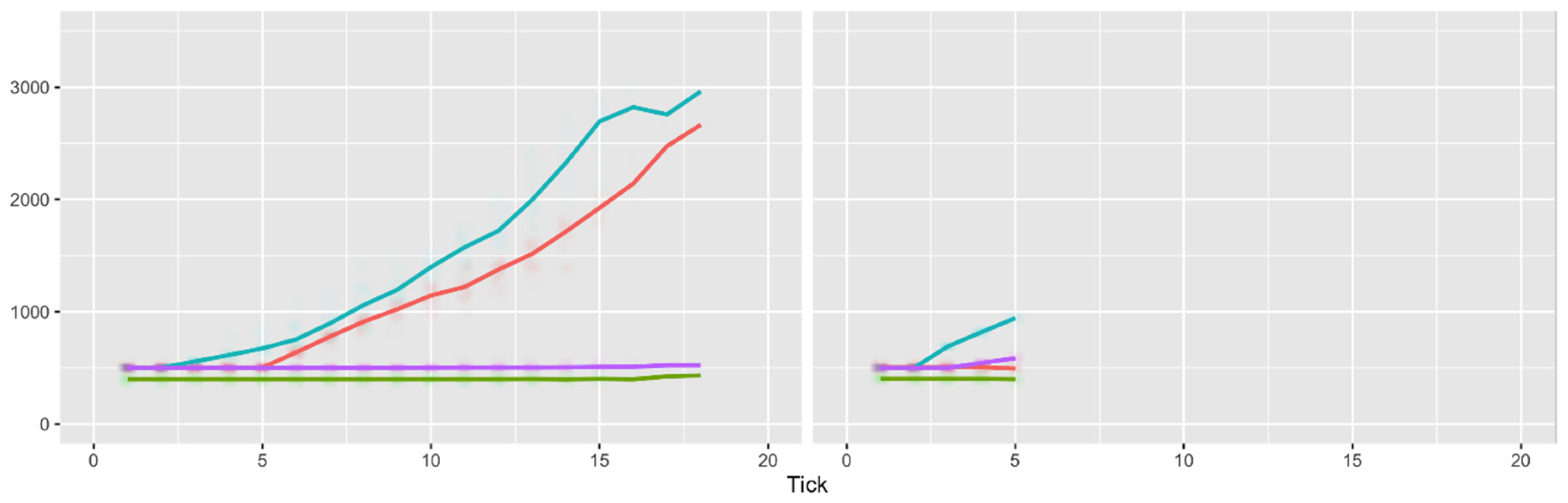
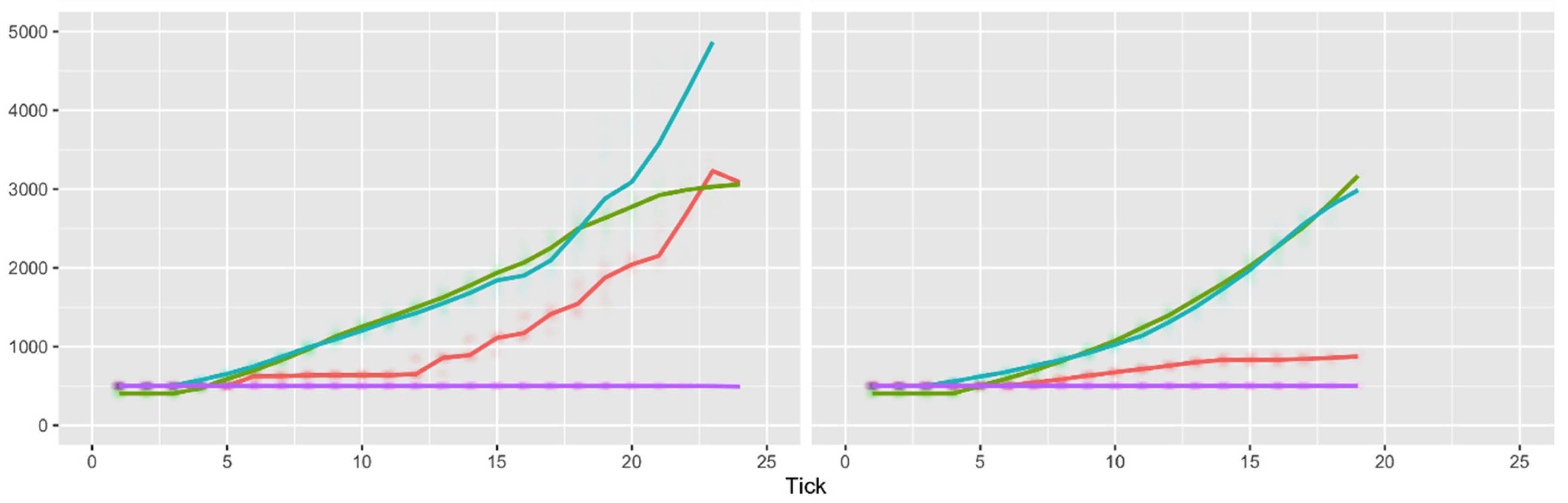
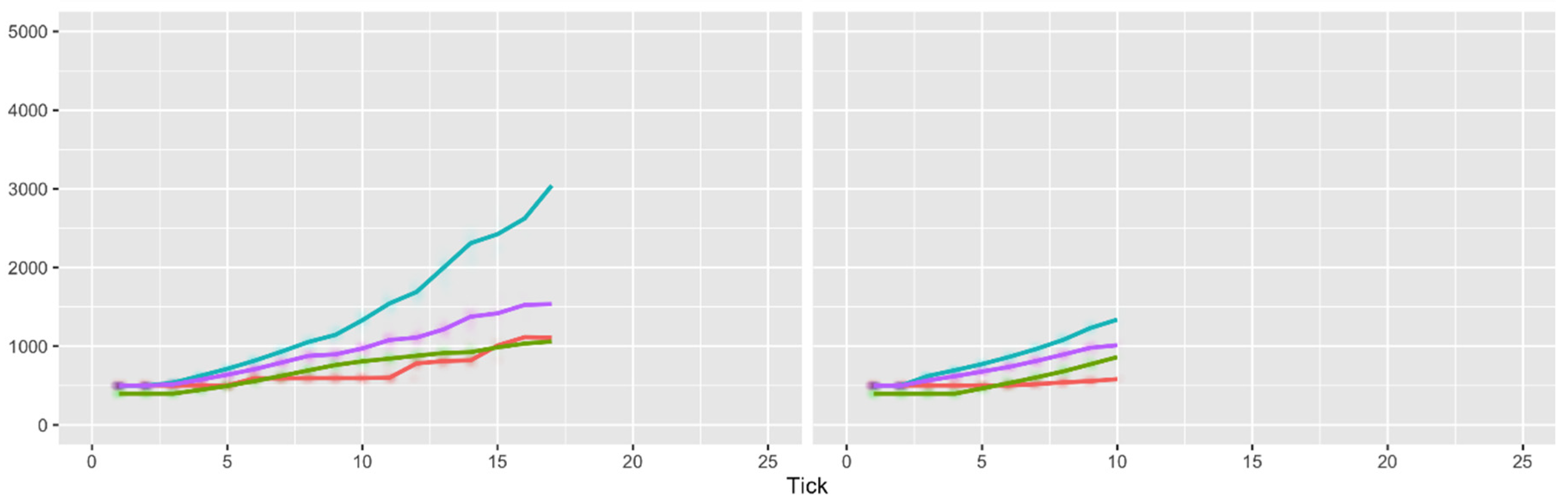
We find that when renewables and fossil fuels are close enough in cost to be competing for investment, the tax has a clear advantage over the ETS. This is because of the ETS’s balancing feedback. This is visible in the results for renewables 1× (Exogenous and Endogenous), and for renewables 2× (Exogenous) and renewables 3× (Exogenous). If the cost difference between renewables and fossil fuels is higher than the carbon price, then there is little that the tax can achieve, so its advantage is neutralised. This is seen in the early stages of renewables 3× Endogenous. Whether the ETS has more effect in this context depends on its design: it can have more effect than the tax if it imposes a high penalty for emissions in excess of the cap (as seen in the early stages of renewables 3× Endogenous).

If innovation is endogenous and the carbon price is too low compared to the cost difference between renewables and fossil fuels, then it will be difficult for either form of carbon pricing to be effective early in the transition. This is the case at the beginning of the 3× Endogenous scenario. The tax can only be effective when the cost difference reduces, which could take a long time if there is minimal renewable deployment (and therefore slow progress down the learning curve). The ETS will eventually force a transition either by imposing penalties for exceeding the emissions cap or by generating a higher carbon price as the cap falls over time, but as it does so, its balancing feedback begins to work against it. In our experiment, where we have set the tax to equal the average ETS price, the tax policy completes the transition faster than the ETS, but with less of an advantage in 3× Endogenous than in 1× Endogenous. In reality, a better policy would be to set the tax equal to the cost difference at the beginning of the transition so that it is effective immediately. Without being encumbered by the balancing feedback, the tax would then outperform the ETS by a larger margin, as we see in the renewables 1× scenarios.

If innovation is exogenous, then renewables and fossil fuels will be brought into competition with each other sooner or later, whatever the starting values of the cost difference and the carbon price. The tax is able to take advantage of this cost reduction by further closing (and reversing) the cost difference, pushing a faster transition. The ETS is encumbered by its balancing feedback, which limits its ability to contribute to the closing of the cost difference beyond what is being achieved by the exogenous renewable cost reduction. We see this significant advantage of the tax in the renewable 3× Exogenous and renewable 2× Exogenous scenarios. These scenarios could be representative of the situation of a country that has a small share of the global market for a clean technology, and where the main components of cost reduction are global rather than local. If a country has a relatively large share of the global market for a clean technology, or if the main components of cost reduction are local, then there may be no strong exogenous cost reduction trend to harness. However, if clean technology deployment subsidies are used in a context of endogenous innovation, this can produce a cost reduction trend, which the tax will be better able to build on than the ETS (similar to what we see in the renewables 3× Exogenous and renewables 2× Exogenous scenarios). 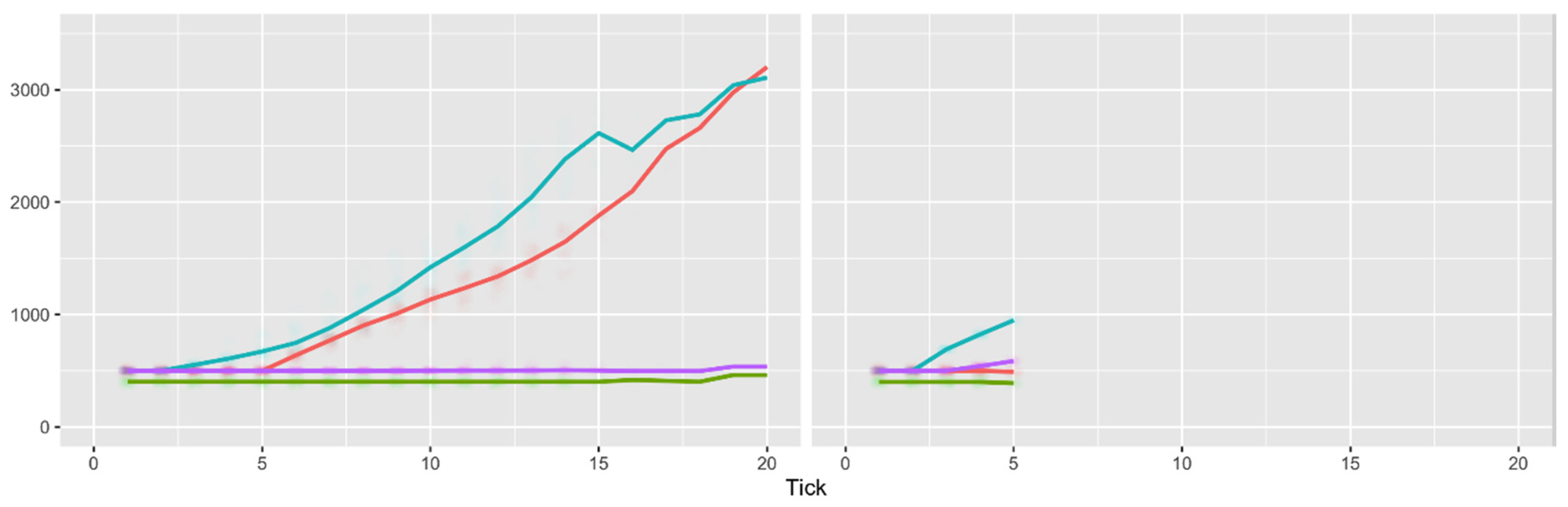See Table 2 and Figure 4, Figure 5, Figure 6 and Figure 7 for the results comparing exogenous and endogenous innovations with different initial renewable energy investment costs (3× and 1×).

In any of our scenarios where the cost difference between renewables and fossil fuels is high, we see that the main effect of either form of carbon pricing is to drive a coal-to-gas switch, with deployment of renewables delayed until their costs have reduced. This leads to significant ‘wasted’ fossil fuel investment over the course of the transition and is consistent with other research that suggests clean technology subsidies can be a more cost-effective way to drive the transition, especially in its early stages. As shown in Table 2, cumulative investment in coal power capacity is much higher under the ETS policy than under the tax, in each of the pairs of scenarios. This is a consequence of the balancing feedback of the ETS, which allows investment in coal capacity to occur whenever carbon prices are low. For the same reason, cumulative emissions are always higher under the ETS than under the tax, even when the time taken to reach zero emissions is similar.

As for testing the effect of halving the innovation rates for renewable technologies, we introduced this test by dividing by 2 the β in Equation (1). We found that the results are as expected, with an increase in mean time for emissions to get to zero, an increase in mean energy prices and an increase in the cumulative emissions across scenarios. Halving the innovation rate also sees a slightly larger impact on the Tax run (in terms of taking longer to get to zero emissions) than on the ETS run. Therefore, we can conclude that a faster innovation rate results in Tax having a larger advantage over the ETS. This appears consistent with the interpretation of the systems mapping (see Section 3): the more powerful the reinforcing feedback between technology deployment and cost reduction, the greater the losses that arise from the offsetting interaction between this feedback and the balancing feedback of the ETS.

Finally, we tested the effect of the ETS cap reduction rate on the results of the model. As mentioned in the previous section, the baseline parameter used for the ETS cap reduction was 2.2%, in line with the EU ETS. In our tests, we ran simulations with this parameter set at 1.2% and 3.2%. When set at 1.2%, the median ETS carbon price was £33, which was slightly below the £34 from the baseline simulations. This is to be expected as a slower cap reduction should result in a lower ETS price, as the drive to get to zero emissions is less strong. The differences were not particularly stark in many of the observed variables; however, the mean values for the ETS price (as opposed to the median) were noticeably different, with a slightly higher mean for the ETS with 2.2% cap reduction (i.e., £55.5) as compared with the other scenario (i.e., £51.6). When comparing the ETS scenario with the ETS cap reduction set at 3.2%, we found that the ETS price was £61.3 (mean) compared with the ETS with a 2.2% cap reduction, with a mean of £55.5.

As is to be expected, the cumulative emissions were also different across the three different scenarios. For the results from these tests, the model can be said to be fairly sensitive to the rate of ETS cap reduction.

All other parameters do not have such a strong impact on the model dynamics and therefore on the results. Therefore, we keep these parameters constant in the runs that were used to present our results below.

5.2. Results for the Comparison of the Policy Options

To ensure the results of our comparison of the policy options are robust, we ran the model using the 1× renewable energy investment costs with endogenous innovation with the three possible scenarios (i.e., BAU, ETS and Tax), with the same plausible values for key parameters as those listed in Section 4.8, over 100 repetitions for each combination of parameters for a total of 900 runs.

Table 3. Results from the model with parameters set following Section 4.8.

Variable	Scenario	Minimum Value	Median Value	Mean Value	Maximum Value
Time emissions reached 0 (years/ticks)	BAU	48	48	48	48
	ETS	11	15	15	24
	Tax	4	6	6	12
Electricity prices (€/MWh)	BAU	20.10	21.80	26.86	50.43
	ETS	24.06	49.37	43.15	71.54
	Tax	49.34	53.62	53.02	54.23
Cumulative emissions (Mt CO2)	BAU	3122	354,763	547,006	1,958,519
	ETS	3172	29,709	32,388	114,929
	Tax	2979	9294	9028	21,834
ETS price (€)	ETS	0	33.73	55.59	727.76

shows the results from the simulations.

From the results shown in Table 3, it is clear that a carbon tax achieves zero emissions in the shortest amount of time, with a median time value of less than half that of the ETS. Average cumulative emissions were also about three times higher under the ETS than under the carbon tax.

6. Discussion

Bringing together the findings from the theoretical review, systems thinking analysis, and agent-based model simulation, we can observe some commonalities and differences and draw out implications for carbon pricing, policy analysis, and decarbonisation policy in general.

Our findings from a stylised ABM applied to an electricity market suggest that, for the same average carbon price, a tax is likely to reduce emissions faster than a cap-and-trade policy, and lead to lower cumulative carbon emissions over time, as well as lower cumulative investment in fossil fuel generation capacity (in particular coal), much of which could be stranded at the end of the transition. The core dynamic driving this difference is the balancing feedback that exists within the cap-and-trade policy but not within the tax. Under the cap-and-trade policy, investment in renewables reduces demand for emissions permits, lowering the permit price and reducing the incentive for further such investment. The path dependence of the system prevents the same average carbon price from having the same effect with each of the two policies. Investments in fossil fuel plants made when the ETS price is low create assets that will be operated for as long as they are profitable, and deplete cash reserves that could be used for investments in renewables.

We find that the relative performance of the two policies is influenced by the interplay of the cost differences between technology options and the presence of endogenous or exogenous innovation. The speed advantage of the tax in reaching zero emissions is greatest when the cost difference between renewables and fossil fuels is small, and under conditions of endogenous innovation, this advantage is increased when the technology learning curve is steeper. The speed advantage of the tax is the least (though still substantial) in the situation where the cost difference between renewables and fossil fuels is high, and innovation is endogenous, but it is in this same scenario that the cap-and-trade policy leads to the highest levels of potentially wasted investment in fossil fuel assets.

In practice, the effectiveness of either of these policies will be strongly influenced by the specifics of their design and implementation, as well as by their interactions with other policies that may provide incentives (such as research and development support or deployment subsidies) or barriers (such as restrictions within planning regulations). However, the fundamental differences between them, in terms of the feedback they create, suggest that the default preference should be for a tax. In the Supplementary Material, we show that the advantage of a tax over an ETS may be greater when used in combination with other renewable energy innovation or deployment policies.

We note that we do not model the distributional impacts of either policy. Further policy measures to mitigate the impact of increases in electricity price through cross-subsidy or alternative pricing measures, as well as routes to manage the distributional impact of returns on investment in renewables, are beyond the scope of this paper, but we highlight their importance here. Neither do we consider the enforceability of either policy, its flexibility, or its suitability for any particular national contexts. Our comparison is limited to the policies’ effectiveness in meeting their primary objective.

This study shows the value for policy analysis of techniques that do not rely on assumptions of no path dependence, equilibrium, or extrapolation. The abandonment of these assumptions was necessary to allow a comparison of the dynamic effectiveness of the policy options. This is likely to be true for any problem of decarbonisation policy, given the limited conditions in which those assumptions are valid and the incompatibility of those conditions with a situation in which the aim is to contribute to a low-carbon system transition.

In the traditional view, either a cap-and-trade policy or a carbon tax is thought to achieve ‘decarbonisation at least cost’ [5], because they allow emissions reductions to be made at the lowest marginal cost of abatement. We have found that the policies are not the same in this respect. Both policies incentivise a firm to make a least-cost emissions reduction at a given moment in time, but the cap-and-trade policy is not the least cost over a period of time. In particular, under the cap-and-trade policy, if any progress beyond the minimum required is achieved at one point in time, then the policy reduces the marginal abatement required at the next moment in time. The cap-and-trade policy achieves the minimum emissions reductions that it requires, whereas the tax achieves a much steeper reduction for the same average carbon price.

The modelling findings are consistent with the insight from the systems mapping that the tax is the more dynamically effective policy: it achieves faster and larger emissions reductions for a given level of intervention, and leads to less potentially wasted investment in fossil fuel assets. Having abandoned the assumption that allocative and dynamic efficiency are equivalent, this suggests a new hypothesis: that in the early stages of a low-carbon transition, the relationship between the two is inverse.

Options for achieving emissions reductions can be divided into two categories [52]. Some actions bring emissions reductions that are immediate but temporary—for example, running coal plants for fewer hours and gas plants for more hours. We refer to these as ‘operational adjustments’. Others, which we call ‘capital replacements’, bring emissions reductions that are permanent—for example, installing solar or wind plants instead of coal or gas. A low-carbon transition whose goal is zero emissions at the sector level involves the replacement of the entire capital stock—from high-carbon assets to zero-carbon assets. This may be done quickly or slowly, but it cannot be avoided. To a first, very rough, approximation, we can consider this process to involve a fixed total amount of investment in capital replacements. Once it is done, it is only the maintenance costs of the zero-carbon capital stock that are required to ensure continued zero emissions.

In principle, for a transition that is to be achieved within a given timeframe, the lowest overall costs are likely to be achieved by maximising the proportion of spending that goes into capital replacements and minimising the proportion that goes into operational adjustments. This will tend to minimise unnecessary spending on emissions reductions that are not permanent (as well as reducing wasted investment in fossil fuel assets).

This is likely to require overcoming a significant cost difference in favour of emissions reduction through operational adjustments. Operational adjustments are likely to be a relatively low-cost way to reduce emissions at the beginning of a transition, because they can be implemented within the incumbent socio-technical regime—i.e., no structural change is required. However, there is no strong reason to expect their cost to change over time. In contrast, zero-emissions capital stock, or clean technology, is likely to be high cost at the start of the transition, when it is relatively immature. Initial investments in capital replacement will yield little in terms of emissions reductions, but will be crucial to begin the process of transition. Unless there are no economies of scale or learning, the cost of clean technology will fall over the course of the transition. We would therefore expect the greatest cost difference (per unit of emissions reduced) between capital replacement (higher cost) and operational adjustments (lower cost) to exist at the beginning of the transition, and for this difference to decrease gradually over the course of the transition.

This is consistent with observations. Early in the global power sector transition, deploying new zero-emission generating capacity was vastly more expensive than replacing coal with gas, in terms of pounds per tonne of avoided emissions. In 2014, analysis showed that switching from coal to gas offered the cheapest marginal abatement option for the US power system, whereas deploying solar power was the most expensive option [53]. But the costs of solar and wind power have fallen by constant fractions [54] with each doubling of deployment, while no long-term trend is observable in the costs of coal or gas. Solar and wind are now the cheapest forms of new power generation in almost all countries [55]. In leading markets, installing new solar and wind is becoming cheaper than continuing to operate existing coal or gas plants [55].

Given this trajectory of relative costs, achieving the transition at the least cost over a given time period generally requires the highest-cost marginal abatements to be made at the beginning. A policy that incentivises least-cost marginal abatement at each moment in time does the opposite. It will tend to maximise spending on operational adjustments—preferring these for as long as they are cheaper—and so cause the transition to be completed at maximum cost overall.

If this logic holds for cap-and-trade within one sector in one country, then the error will be compounded if the policy is expanded to cover more sectors or more countries. The broader the coverage of the cap-and-trade, the more opportunities there will be for operational adjustments that have a lower marginal cost than capital replacements. The more these opportunities are exploited in preference to the more expensive but necessary investments in capital replacements, the more additional costs there will be for the transition overall, and the more delayed that transition will be.

Limitations

As mentioned previously in the text, the main limitation of the model is its stylised nature, aimed at illustrating the relationships highlighted in the systems map in a dynamic environment, while introducing measures to address limitations present in other models (e.g., equilibrium dynamics and exogenous innovation). The stylised model made a series of assumptions that inevitably have an impact on the dynamics represented in the model and on the results that we found. The justification for most of these assumptions is to keep the model as simple as possible but not overly simple.

Some of the key simplifications made are, for instance, the synthetic electricity market with a random number of companies, which are assigned a random amount of GW capacity for all technologies included in the simulations, a demand approximated by an exogenous trendline, and a system where companies do not install power stations but rather create new capacity in batches. In particular, this last assumption could affect the system through the economics of depreciation and decommissioning, as we had to highly simplify these dynamics in the model.

An additional limitation is that the model presented here focuses on only two policy options—a carbon price in the form of an emissions trading system or a tax. We do not account for interactions with other policies, such as subsidies, regulations, research and development funding, or infrastructure investment (except through the qualitative system mapping, as set out in the Supplementary Material). In reality, all these and other policies can be important for the development and deployment of clean technologies. We focused the modelling in this way so as to examine the different dynamic effects of a carbon tax compared to an emissions trading system. One consequence is that the innovation represented in the model includes the learning effects of technology deployment but not the early-stage innovation or early-stage deployment (when technologies are far from being cost-competitive). Further research could usefully explore the dynamic effects of a wider range of policies implemented individually and in differing combinations.

In implementing a carbon tax, we opted to set this as the average carbon price across the ETS run of the model. Whilst this allows for comparison between the two policies with the same average carbon price, it does not model for flexibility in carbon tax implementation (for example, carbon taxes could be set low and ramp up with future foresight, allowing markets to plan, or start high and then decline as the cost difference between clean technologies and fossil fuels reduces). Similarly, the rate of reduction in the emissions cap of an ETS can be changed over time, as has been the case in the EU ETS. We used the simplest versions of both policies to enable a clear comparison.

A further limitation is in the choice of some behaviour parameters in the model—especially in how companies perceive the relative benefits of investing in renewables or fossil fuel solutions. In future, the model itself could be used to calibrate these parameters by exploring outputs against real-world data, or an expert elicitation of a sufficient portion of the market could be conducted to gather this behavioural data. However, we also note that this behaviour is likely to change with time as the market develops and technologies are deployed, and therefore these parameters could evolve. While this is a limitation in the model, it does not affect the model’s findings on the relative effectiveness of the two policy options in a qualitative way.

We also note that the model assumes a closed, competitive electricity market without cross-regional trade, policy heterogeneity, or institutional differences. This is a significant simplification of the reality of energy systems. In reality, many such factors influence the effectiveness of any policy options.

7. Conclusions

In this paper, we present a stylised agent-based model designed to investigate the difference between two alternative policy options for carbon pricing under conditions of endogenous or exogenous innovation.

We find that a carbon tax generally achieves faster emissions reduction, lower cumulative emissions, and less cumulative (potentially wasted) investment in fossil fuel assets than a cap-and-trade policy. The findings indicate the relevance of dynamic forms of analysis for comparing policies for the low-carbon transition.

In this context, we see that the ABM’s freedom from the constraints of the assumptions of no-path dependence, equilibrium, and extrapolation allows it to explore dynamic effects that are important to the performance of the two policy options. There is path dependence in the way that agents’ investing in higher-cost technologies brings down the costs of those technologies and makes them more profitable, changing the calculations in future decisions. Disequilibrium arises from the heterogeneous behaviours of individual companies (distributed around a norm) interacting with technological change in a context of uncertainty. These interactions produce the feedback effects that differentiate the two policies’ performance. Finally, the model’s use of multiple agents with a spread of behaviours rather than a single ‘representative agent’ means it makes no assumption of extrapolation. The findings illustrate the potential for different behaviour at the system level even when the decision-making rules of the agents are unchanged.

The stylised agent-based model presented here could usefully be further developed to include the wider dynamics of the market, to test a wider variety of policy options, and to more accurately reflect the specific conditions of electricity markets in the EU or other regions.